Domination Number of an Interval Catch Digraph Family and Its Use for Testing Uniformity

Abstract

We consider a special type of interval catch digraph (ICD) family for one-dimensional data in a randomized setting and propose its use for testing uniformity. These ICDs are defined with an expansion and a centrality parameter, hence we will refer to this ICD as parameterized ICD (PICD). We derive the exact (and asymptotic) distribution of the domination number of this PICD family when its vertices are from a uniform (and non-uniform) distribution in one dimension for the entire range of the parameters; thereby determine the parameters for which the asymptotic distribution is non-degenerate. We observe jumps (from degeneracy to non-degeneracy or from a non-degenerate distribution to another) in the asymptotic distribution of the domination number at certain parameter combinations. We use the domination number for testing uniformity of data in real line, prove its consistency against certain alternatives, and compare it with two commonly used tests and three recently proposed tests in literature and also arc density of this ICD and of another ICD family in terms of size and power. Based on our extensive Monte Carlo simulations, we demonstrate that domination number of our PICD has higher power for certain types of deviations from uniformity compared to other tests.

short title: Domination Number of an ICD Family for Testing Uniformity

Keywords: arc density; asymptotic distribution; class cover catch digraph; consistency; exact distribution; proximity catch digraph; uniform distribution

AMS 2000 Subject Classification: 05C80; 05C20; 60D05; 60C05; 62E20

1 Introduction

Graphs and digraphs for one dimensional points as vertices have been extensively studied and have far-reaching applications despite their simplicity. In this article, we introduce an interval catch digraph (ICD) family, provide the distribution of its domination number for random vertices, and employ the domination number in testing uniformity of one-dimensional data. Interval graphs and digraphs have applications in many fields such as chronological ordering of artifacts in archeology, modeling traffic lights in transportation, food web models in ecology, document localization, classification of RNA structures and so on (see Roberts, (1976), Drachenberg, (1994), Arlazarov et al., (2017), and Quadrini et al., (2017)). ICDs were introduced as a special type of interval digraphs and found applications in various fields (see Prisner, (1989, 1994) for a characterization and detailed discussion of ICDs). The new digraph family we consider in this article is parameterized by an expansion parameter and a centrality parameter. We demonstrate that this digraph family is actually an ICD family, hence it is referred to as parameterized ICD (PICD). A digraph is a directed graph with vertex set $\mathcal{V}$ and arcs (directed edges) each of which is from one vertex to another based on a binary relation. The pair $(p,q)\in\mathcal{V}\times\mathcal{V}$ is an ordered pair which stands for an arc from vertex $p$ to vertex $q$ in $\mathcal{V}$.

The PICDs are closely related to the class cover problem (CCP) of Cannon and Cowen, (2000) which is motivated by applications in statistical classification. To properly describe the CCP problem, let $(\Omega,d)$ be a metric space with a dissimilarity function $d:\Omega\times\Omega\rightarrow\mathbb{R}$ such that $d(a,b)=d(b,a)\geq d(a,a)=0$ for all $a,b\in\Omega$. Let $\mathcal{X}_{n}=\{X_{1},X_{2},\ldots,X_{n}\}$ and $\mathcal{Y}_{m}=\{Y_{1},Y_{2},\ldots,Y_{m}\}$ be two sets of i.i.d. $\Omega$-valued random variables from classes $\mathcal{X}$ and $\mathcal{Y}$, with class-conditional distributions $F_{X}$ and $F_{Y}$, respectively. We also assume that each $X_{i}$ is independent of each $Y_{j}$ and all $X_{i}\in\mathcal{X}_{n}$ and all $Y_{j}\in\mathcal{Y}_{m}$ are distinct with probability one, and $(X_{i},Y_{j})\sim F_{X,Y}$ (i.e., $(X_{i},Y_{j})$ has joint distribution $F_{X,Y}$ with the marginal distributions $F_{X}$ for $X_{i}$ and $F_{Y}$ for $Y_{j}$). The CCP for a target class refers to finding a collection of neighborhoods, $\mathcal{N}$ around $X_{i}$, denoted $N(X_{i})\in\mathcal{N}$, such that (i) $\mathcal{X}_{n}\subseteq\bigl{(}\cup_{i}N(X_{i})\bigr{)}$ and (ii) $\mathcal{Y}_{m}\cap\bigl{(}\cup_{i}N(X_{i})\bigr{)}=\emptyset$. The neighborhood $N(X_{i})$ is a subset of $\Omega$, containing $X_{i}$, and is defined based on the dissimilarity $d$ (between $X_{i}$ and $\mathcal{Y}_{m}$). A collection of neighborhoods satisfying both conditions is called a class cover. Clearly, it follows by condition (i) that the set of all covering regions (i.e., neighborhoods $N(X_{i})$ around $X_{i}$) is a class cover; however, the goal is to have a class cover for $\mathcal{X}_{n}$ that has as few points as possible. Thus, e.g. in statistical learning, the classification will be less complex while most of the relevant information being kept. Hence, the CCP considered here is a minimum-cardinality class cover. One can convert the CCP to the graph theoretical problem of finding dominating sets. In particular, our ICD is the digraph $D=(\mathcal{V},\mathcal{A})$ with vertex set $\mathcal{V}=\mathcal{X}_{n}$ and arc set $\mathcal{A}$ such that there is an arc $(X_{i},X_{j})\in\mathcal{A}$ iff $X_{j}\in N(X_{i})$. It is easy to see that solving the CCP is equivalent to finding a minimum domination set of the corresponding PICD, hence cardinality of a solution to CCP is equal to the domination number of the associated digraph (see Marchette, (2004)). Hence the tool introduced in this article can be seen as a parameterized extension to the original CCP problem of Cannon and Cowen, (2000). That is, the cardinality of the smallest cover (i.e., the domination number) is investigated when the cover(ing) regions, $N(X_{i})$, depend on two parameters and the distribution of this cardinality is based on $N(X_{i})$ (hence the parameters) and $F_{X,Y}$.

Our PICDs are random digraphs (according to the digraph version of classification of Beer et al., (2011)) in which each vertex corresponds to a data point and arcs are defined in terms of some bivariate relation on the data, and are also related to the class cover catch digraph (CCCD) introduced by Priebe et al., (2001) who derived the exact distribution of its domination number for uniform data from two classes in $\mathbb{R}$. A CCCD consists of a vertex set in $\mathbb{R}^{d}$ and arcs $(u,v)$ if $v$ is inside the ball centered at $u$ with a radius based on spatial proximity of the points. CCCDs were also extended to higher dimensions and were demonstrated to be a competitive alternative to the existing methods in classification (see DeVinney and Priebe, (2006) and references therein) and to be robust to the class imbalance problem (Manukyan and Ceyhan, (2016)). Furthermore, a CLT result for CCCD based on one-dimensional data is proved (Xiang and Wierman, (2009)) and the distribution of the domination number of CCCDs is also derived for non-uniform data (Ceyhan, (2008)).

We investigate the distribution of domination number of the PICDs for data in $\Omega=\mathbb{R}$. The domination in graphs has been studied extensively in recent decades (see, e.g., Hedetniemi and Laskar, (1990) and the references therein and Henning and Yeo, (2013)), and domination in digraphs has received comparatively less attention but is also studied in literature (see, e.g., Lee, (1998), Niepel and Knor, (2009) and Hao, (2017)). We provide the exact and asymptotic distributions of the domination number of PICDs with vertices from uniform (and non-uniform) one-dimensional distributions. Some special cases and bounds for the domination number of PICDs are handled first, then the domination number is investigated for uniform data in one interval (in $\mathbb{R}$) and the analysis is generalized to uniform data in multiple intervals and to non-uniform data in one and multiple intervals.

We use domination number in testing uniformity of one-dimensional data. Testing uniformity is important in its own right in numerous fields, e.g., in assessing the quality of random number generators (L’Ecuyer, (2001)) and in chemical processes (Fahidy, (2013)). Furthermore, testing that data come from a particular distribution can be reduced to testing uniformity, hence uniformity tests are of great importance for goodness-of-fit tests (see Milošević, (2018) and references therein). Some graph theoretical tools are employed (although not so commonly) in two-sample testing (Chen and Friedman, (2017) and in testing uniformity; for example, Jain et al., (2002) use minimum spanning trees and Ceyhan, (2016) use the arc density of another family of ICDs for this purpose. Moreover, Ceyhan, (2012) provide the probabilistic investigation of the arc density for the PICD of this article, but it is not applied for uniformity testing previously. In (Ceyhan, (2008)), the distribution of the domination number of CCCDs is studied when vertices are from a non-uniform one-dimensional distribution, but the domination number of the PICD introduced here is not studied previously. To the author’s knowledge domination number is not used in literature for testing uniformity. We compare the size and power performance of our test with two well known competitors, namely Kolmogorov-Smirnov (KS) test and Pearson’s $\chi^{2}$ goodness-of-fit test, and the arc density of PICDs and of another ICD family, and also a uniformity test which is based on Too-Lin characterization of the uniform distribution due to Milošević, (2018), and two entropy-based tests due to Zamanzade, (2015). We demonstrate that the test based on the domination number has higher power for certain types of deviations from uniformity. Furthermore, this article forms the foundation of the extensions of the methodology to higher dimensions. The domination number has other applications, e.g., in testing spatial point patterns (see, e.g., Ceyhan and Priebe, (2005)) and our results can help make the power comparisons possible for a large family of alternative patterns in such a setting. Some trivial proofs regarding PICDs are omitted, while others are mostly deferred to the Supplementary Materials Section.

We define the PICDs and their domination number in Section 2, provide the exact and asymptotic distributions of the domination number of PICDs for uniform data in one interval in Section 3, discuss the distribution of the domination number for data from a general distribution in Section 4. We extend these results to multiple intervals in Section 5, use domination number in testing uniformity in Section 6, prove consistency of the domination number tests under certain alternatives in Section 7, and provide discussion and conclusions in Section 8.

2 A Parameterized Random Interval Catch Digraph Family

Let $N:\Omega\rightarrow\wp(\Omega)$ be a map where $\wp(\Omega)$ represents the power set of $\Omega$. Then the proximity map $N(\cdot)$ associates with each point $x\in\Omega$ a proximity region $N(x)\subseteq\Omega$. For $B\subseteq\Omega$, the $\Gamma_{1}$-region is the image of the map $\Gamma_{1}(\cdot,N):\wp(\Omega)\rightarrow\wp(\Omega)$ that associates the region $\Gamma_{1}(B,N):=\{z\in\Omega:B\subseteq N(z)\}$ with the set $B$. For a point $x\in\Omega$, for convenience, we denote $\Gamma_{1}(\{x\},N)$ as $\Gamma_{1}(x,N)$. Notice that while the proximity region is defined for one point, a $\Gamma_{1}$-region can be defined for a set of points. The PICD has the vertex set $\mathcal{V}=\mathcal{X}_{n}$ and arc set $\mathcal{A}$ defined by $(X_{i},X_{j})\in\mathcal{A}$ iff $X_{j}\in N(X_{i})$.

Although the above definition of the proximity region does not require multiple classes, in this article, we will define proximity regions in a two-class setting based on relative allocation of points from one class (say $\mathcal{X}$) with respect to points from the other class (say $\mathcal{Y}$). We now get more specific and restrict our attention to $\Omega=\mathbb{R}$ and define $N$ explicitly. Let $\mathcal{Y}_{m}$ consist of $m$ distinct points from class $\mathcal{Y}$ and $Y_{(i)}$ be the $i^{th}$ order statistic (i.e., $i^{th}$ smallest value) of $\mathcal{Y}_{m}$ for $i=1,2,\ldots,m$ with the additional notation for $i\in\{0,m+1\}$ as

$$-\infty=:Y_{(0)}<Y_{(1)}<\ldots<Y_{(m)}<Y_{(m+1)}:=\infty.$$

Then $Y_{(i)}$ values partition $\mathbb{R}$ into $(m+1)$ intervals which is called the intervalization of $\mathbb{R}$ by $\mathcal{Y}_{m}$. Let also that $\mathcal{I}_{i}:=\left(Y_{(i)},Y_{(i+1)}\right)$ for $i\in\{0,1,2,\ldots,m\}$ and $M_{c,i}:=Y_{(i)}+c\left(Y_{(i+1)}-Y_{(i)}\right)$ (i.e., $M_{c,i}\in\mathcal{I}_{i}$ such that $c\times 100$ % of length of $\mathcal{I}_{i}$ is to the left of $M_{c,i}$). We define the parameterized proximity region with the expansion parameter $r\geq 1$ and centrality parameter $c\in[0,1]$ for two one-dimensional data sets, $\mathcal{X}_{n}$ and $\mathcal{Y}_{m}$, from classes $\mathcal{X}$ and $\mathcal{Y}$, respectively, as follows (see also Figure 1). For $x\in\mathcal{I}_{i}$ with $i\in\{1,2,\ldots,m-1\}$ (i.e. for $x$ in the middle intervals)

$$N(x,r,c)=\begin{cases}\left(Y_{(i)},\min\left(Y_{(i+1)},Y_{(i)}+r\,\left(x-Y_{(i)}\right)\right)\right)&\text{if $x\in(Y_{(i)},M_{c,i})$,}\\ \left(\max\left(Y_{(i)},Y_{(i+1)}-r\left(Y_{(i+1)}-x\right)\right),Y_{(i+1)}\right)&\text{if $x\in\left(M_{c,i},Y_{(i+1)}\right)$.}\end{cases}$$ (1)

Additionally, for $x\in\mathcal{I}_{i}$ with $i\in\{0,m\}$ (i.e. for $x$ in the end intervals)

$$N(x,r,c)=\begin{cases}\left(Y_{(1)}-r\left(Y_{(1)}-x\right),Y_{(1)}\right)&\text{if $x<Y_{(1)}$,}\\ \left(Y_{(m)},Y_{(m)}+r\,\left(x-Y_{(m)}\right)\right)&\text{if $x>Y_{(m)}$.}\end{cases}$$ (2)

Figure 1: Illustrations of the construction of the parameterized proximity region, $N(x,r,c)$ with $c\in(0,1/2)$ for $\mathcal{Y}_{2}=\{y_{1},y_{2}\}$ with $y_{1}=0$ and $y_{2}=10$ (hence $M_{c}=10c$) and $x\in(0,M_{c})$ (top) and $x\in(M_{c},10)$ (bottom).

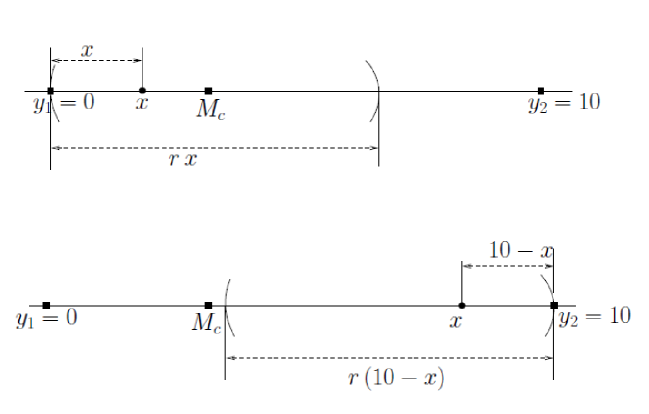
Notice that for $i\in\{0,m\}$, the proximity region does not have a centrality parameter $c$. For $x\in\mathcal{Y}_{m}$, we define $N(x,r,c)=\{x\}$ for all $r\geq 1$ and $c\in[0,1]$. If $x=M_{c,i}$, then in Equation (1), we arbitrarily assign $N(x,r,c)$ to be one of the defining intervals. For $c=0$, we have $\left(M_{c,i},Y_{(i+1)}\right)=\mathcal{I}_{i}$ and for $c=1$, we have $(Y_{(i)},M_{c,i})=\mathcal{I}_{i}$. So, we set $N(x,r,0):=\left(\max\left(Y_{(i)},Y_{(i+1)}-r\left(Y_{(i+1)}-x\right)\right),Y_{(i+1)}\right)$ and $N(x,r,1):=\left(Y_{(i)},\min\left(Y_{(i+1)},Y_{(i)}+r\,\left(x-Y_{(i)}\right)\right)\right)$. For $r>1$, we have $x\in N(x,r,c)$ for all $x\in\mathcal{I}_{i}$. Furthermore, $\lim_{r\rightarrow\infty}N(x,r,c)=\mathcal{I}_{i}$ for all $x\in\mathcal{I}_{i}$, so we define $N(x,\infty,c)=\mathcal{I}_{i}$ for all such $x$.

The PICD has the vertex set $\mathcal{X}_{n}$ and arc set $\mathcal{A}$ defined by $(X_{i},X_{j})\in\mathcal{A}$ iff $X_{j}\in N(X_{i},r,c)$. We denote such PICDs as $\mathbf{D}_{n,m}(F_{X,Y},r,c)$. The randomness of the PICD lies in the fact that the vertices are randomly generated from the distribution $F_{X}$ and proximity regions are random depending on $F_{X,Y}$, but arcs $(X_{i},X_{j})$ are deterministic functions of the random variable $X_{j}$ and the random set $N(X_{i})$. Notice that although $N$ depends on $\mathcal{Y}_{m}$, we omit $\mathcal{Y}_{m}$ for brevity in notation of proximity region $N(x,r,c)$.

2.1 Relation of PICDs with other Graph Families

Interval graphs are a special type of intersection graphs, which have emerged from a problem in genetics called Benzer problem (see Roberts, (1976) for details) and they have been extensively studied in graph theory since their introduction (Drachenberg, (1994) and Francis et al., (2018)). On the other hand, interval digraphs have recently gained attention after their introduction in Sen et al., (1989) (see, e.g., Das et al., (2016)). Let $\mathcal{V}$ be a set of $n$ index points in some arbitrary space; for simplicity take $\mathcal{V}=\{1,2,\ldots,n\}$. Consider a set of “source” intervals $S_{v}$ and a set of “target” intervals $T_{v}$ in $\mathbb{R}$ associated with $v\in\mathcal{V}$. The family of ordered pairs of these intervals $(S_{v},U_{v})_{v\in\mathcal{V}}$ such that $U_{v}\in S_{v}$ for each $v$ is called a nest representation (Prisner, (1994)). The digraph $D=(\mathcal{V},\mathcal{A})$ is called an interval nest digraph, if there exists a nest representation with the index set $\mathcal{V}$ such that $(i,j)\in\mathcal{A}$ iff $S_{i}\cap U_{j}\neq\emptyset$. Interval catch digraphs (ICDs) are interval nest digraphs with each $T_{v}$ containing just one element (Prisner, (1994)). In fact, for catch digraphs the nest representation constitutes a family of sets with points (or pointed sets) $(S_{v},p_{v})_{v\in\mathcal{V}}$ where each set $S_{v}$ is associated with a base point $p_{v}\in S_{v}$. Then $D=(\mathcal{V},\mathcal{A})$ is a catch digraph with $(i,j)\in\mathcal{A}$ iff $p_{j}\in S_{i}$. Such a catch digraph is called an interval catch digraph, if there is a totally ordered set $(T,\leq)$ such that $D$ is the catch digraph of a family of pointed intervals in $T$. Here, $I\subset T$ is an interval if, for all $x,y,z\in T$, $x\leq y\leq z$ and $x,z\in I$ imply that $y\in I$. For finite ICDs, $T$ can always be taken as the real line (see, e.g., Prisner, (1989) who also provides a characterization of ICDs).

The PICDs are closely related to the proximity graphs of Jaromczyk and Toussaint, (1992) and might be considered as one-dimensional versions of proportional-edge proximity catch digraphs of Ceyhan and Priebe, (2005). Furthermore, when $r=2$ and $c=1/2$ (i.e., $M_{c,i}=\left(Y_{(i)}+Y_{(i+1)}\right)/2$) we have $N(x,r,c)=B(x,r(x))$ where $B(x,r(x))$ is the ball centered at $x$ with radius $r(x)=d(x,\mathcal{Y}_{m})=\min_{y\in\mathcal{Y}_{m}}d(x,y)$. The region $N(x,2,1/2)$ corresponds to the proximity region which gives rise to the CCCD of Priebe et al., (2001). Note also that, $N(x,r,c)$ can be viewed as a homothetic transformation (enlargement) with $r\geq 1$ applied on a translation of the region $N(x,1,c)$. Furthermore, this transformation is also an affine similarity transformation. Since $(\mathbb{R},\leq)$ is a total order, by the characterization theorem of Maehara, (1984), our random digraph is clearly an interval catch digraph, since there exists a total order “$\leq$” on $\mathcal{X}_{n}\subset\mathbb{R}$ such that for $x<y<z\in\mathcal{X}_{n}$, $(x,z)\in\mathcal{A}$ implies $(x,y)\in\mathcal{A}$ and $(z,x)\in\mathcal{A}$ implies $(z,y)\in\mathcal{A}$. Our ICD is based on two parameters, so we call it parameterized interval catch digraph (PICD).

2.2 Domination Number of PICDs

In a digraph $D=(\mathcal{V},\mathcal{A})$ of order $|\mathcal{V}|=n$, a vertex $u$ dominates itself and all vertices of the form $\{v:\,(u,v)\in\mathcal{A}\}$. A dominating set, $S_{D}$, for the digraph $D$ is a subset of $\mathcal{V}$ such that each vertex $v\in\mathcal{V}$ is dominated by a vertex in $S_{D}$. A minimum dominating set, $S^{*}_{D}$, is a dominating set of minimum cardinality; and the domination number, denoted $\gamma(D)$, is defined as $\gamma(D):=|S^{*}_{D}|$, where $|\cdot|$ stands for set cardinality (West, (2001)). Chartrand et al., (1999) distinguish domination in digraphs as out- and in-domination and provide definitions for out- and in-domination numbers for digraphs. Domination in this article refers to the out-domination in PICDs. If a minimum dominating set consists of only one vertex, we call that vertex a dominating vertex. Clearly, the vertex set $\mathcal{V}$ itself is always a dominating set, so we have $\gamma(D)\leq n$ in general, and $1\leq\gamma(D)<n$ for nontrivial digraphs.

Let

$$\mathcal{F}\left(\mathbb{R}^{d}\right):=\{F_{X,Y}\text{ on }\mathbb{R}^{d}\text{ with }(X,Y)\sim F_{X,Y},~{}\text{ and random variables X and Y do not collide}\}.$$

That is, if $\mathcal{X}_{n}$ and $\mathcal{Y}_{m}$ are two samples from $F_{X}$ and $F_{Y}$, respectively with $(X,Y)\sim F_{X,Y}$ and the marginal distributions of $X$ and $Y$ are $F_{X}$ and $F_{Y}$, respectively. Furthermore, “no collision of $X$ and $Y$” condition is equivalent to $P(X_{i}=Y_{j})=0$ for all $i=1,\ldots,n$ and $j=1,\ldots,m$. Notice that if $F_{X,Y}$ continuous, then $F_{X,Y}\in\mathcal{F}\left(\mathbb{R}^{d}\right)$ follows. Furthermore, if the probability distributions $F_{X}$ and $F_{Y}$ respectively have probability measures $\mathcal{M}_{X}$ and $\mathcal{M}_{Y}$ which are non-atomic, then the associated joint distribution would be in $\mathcal{F}\left(\mathbb{R}^{d}\right)$ as well. If $\mathcal{M}_{Y}$ contains an atom, $Y_{j}$ points might collide, but without loss of generality we can assume that there are $m$ distinct $\mathcal{Y}$ points. We restrict our attention to one dimensional data (i.e., $d=1$), so we consider the random digraph for which $\mathcal{X}_{n}$ and $\mathcal{Y}_{m}$ are samples from $F_{X}$ and $F_{Y}$, respectively, with the joint distribution of $X,Y$ being $F_{X,Y}\in\mathcal{F}\left(\mathbb{R}\right)$. We focus on the random variable $\gamma(\mathbf{D}_{n,m}(F_{X,Y},r,c))$, the domination number of the digraph $\mathbf{D}_{n,m}(F_{X,Y},r,c)$. To make the notation simpler, we will use $\gamma_{{}_{n,m}}(F_{X,Y},r,c)$ instead of $\gamma(\mathbf{D}_{n,m}(F_{X,Y},r,c))$. For $n\geq 1$ and $m\geq 1$, it is immediate to see that $1\leq\gamma_{{}_{n,m}}(F_{X,Y},r,c)\leq n$.

Let $\mathcal{X}_{[i]}:=\mathcal{X}_{n}\cap\mathcal{I}_{i}$, and $\mathcal{Y}_{[i]}:=\left\{Y_{(i)},Y_{(i+1)}\right\}$ for $i=0,1,2,\ldots,m$. This yields a disconnected digraph with subdigraphs each of which might be null or itself disconnected. Let $\mathbf{D}_{[i]}$ be the component of $\mathbf{D}_{n,m}(F_{X,Y},r,c)$ induced by $\mathcal{X}_{[i]}$ for $i=0,1,2,\ldots,m$, $n_{i}:=\left|\mathcal{X}_{[i]}\right|$ (provided that $n_{i}>0$), and $F_{i}$ be the density $F_{X}$ restricted to $\mathcal{I}_{i}$ (note that $\mathcal{I}_{i}$ is also random here), and $\gamma_{{}_{[i]}}(F_{i},r,c)$ be the domination number of $\mathbf{D}_{[i]}$. Let also that $M_{c,i}\in\mathcal{I}_{i}$ be the internal point that divides the interval $\mathcal{I}_{i}$ in ratios $c/(1-c)$ (i.e., length of the subinterval to the left of $M_{c,i}$ is $c\times 100$ % of the length of $\mathcal{I}_{i}$). Then $\gamma_{{}_{n,m}}(F_{X,Y},r,c)=\sum_{i=0}^{m}\gamma_{{}_{[i]}}(F_{i},r,c)$.

A Summary of Results in this article is as follows:

• In the middle intervals (i.e., for $i=1,2,\ldots,m-1$), we show that $\gamma_{{}_{[i]}}(F_{i},r,c)-1$ has a Bernoulli distribution with the parameter depending on $F_{X,Y}$. In the end intervals (i.e., $i\in\{0,m\}$) where the domination number $\gamma_{{}_{[i]}}(F_{i},r,c)$ is $\mathbf{I}(n_{i}>0)$.

• Conditional on $\mathcal{Y}_{m}$ (i.e., $\mathcal{Y}_{m}$ is given), randomness in the digraph (hence in the domination number) stem from $F_{X}$. So if $\mathcal{Y}_{m}$ is given, we write the corresponding domination number as $\gamma_{{}_{n,m}}(F_{X},r,c)$. In this case, we modify our notations as $\mathbf{D}_{n,m}(F,r,c)$ and $\gamma_{{}_{n,m}}(F,r,c)$ for the PICD and the associated domination number, where $F=F_{X}$.

  • Then we show that $\gamma_{{}_{n,2}}(F,r,c)$ is scale invariant for $\mathcal{Y}_{2}=\{a,b\}$, $F=\mathcal{U}(a,b)$ with $-\infty<a<b<\infty$, where $\mathcal{U}(a,b)$ stands for uniform distribution on $(a,b)$, hence (without loss of generality) we can consider $\mathcal{U}(0,1)$.

  • We find the exact (and hence the asymptotic) distribution of $\gamma_{{}_{n,2}}(\mathcal{U},r,c)$ for $r\geq 1,c\in[0,1]$ (which is the most general case for these parameters).

  • We extend the result in (ii) by considering the general non-uniform $F$ satisfying mild regularity conditions, thereby find the asymptotic distribution of $\gamma_{{}_{n,2}}(F,r,c)$.

  • Finally, we provide the more general form (in terms of $n$ and $m$) of $\gamma_{{}_{n,m}}(F,r,c)$ by considering general $m$ (i.e., $m>2$) and find the asymptotic distribution of $\gamma_{{}_{n,m}}(F,r,c)$.

• Domination number is employed as a test statistic for testing uniformity of one-dimensional data, is consistent and exhibits a good performance for certain types of alternatives.

2.3 Special Cases for the Distribution of $\gamma_{n,m}(F_{X,Y},r,c)$

We study the simpler random variable $\gamma_{{}_{[i]}}(F_{i},r,c)$ first. The following lemma follows trivially.

Lemma 2.1.

For $i\in\{0,m\}$, we have $\gamma_{{}_{[i]}}(F_{i},r,c)=\mathbf{I}(n_{i}>0)$ for all $r\geq 1$. For $i=1,2,3,\ldots,(m-1)$, if $n_{i}=1$, then $\gamma_{{}_{[i]}}(F_{i},r,c)=1$.

Let $\Gamma_{1}\left(B,r,c\right)$ be the $\Gamma_{1}$-region for set $B$ associated with the proximity map $N(\cdot,r,c)$.

Lemma 2.2.

The $\Gamma_{1}$-region for $\mathcal{X}_{[i]}$ in $\mathcal{I}_{i}$ with $r\geq 1$ and $c\in[0,1]$ is

$$\Gamma_{1}\left(\mathcal{X}_{[i]},r,c\right)=\Biggl{(}\frac{\max\,\left(\mathcal{X}_{[i]}\right)+Y_{(i)}(r-1)}{r},M_{c,i}\Biggr{]}\bigcup\Biggl{[}M_{c,i},\frac{\min\left(\mathcal{X}_{[i]}\right)+Y_{(i+1)}(r-1)}{r}\Biggr{)}$$

with the understanding that the intervals $(a,b)$, $(a,b]$, and $[a,b)$ are empty if $a\geq b$.

Notice that if $\mathcal{X}_{[i]}\cap\Gamma_{1}\left(\mathcal{X}_{[i]},r,c\right)\not=\emptyset$, we have $\gamma_{{}_{[i]}}(F_{i},r,c)=1$, hence the name $\Gamma_{1}$-region and the notation $\Gamma_{1}(\cdot)$. For $i=1,2,3,\ldots,(m-1)$ and $n_{i}>1$, we prove that $\gamma_{{}_{[i]}}(F_{i},r,c)=1$ or $2$ with distribution dependent probabilities. Hence, to find the distribution of $\gamma_{{}_{[i]}}(F_{i},r,c)$, it suffices to find the probability of $\gamma_{{}_{[i]}}(F_{i},r,c)$ is 1 or 2. For computational convenience, we employ the latter in our calculations henceforth and denote it as $p(F_{i},r,c):=P\bigl{(}\gamma_{{}_{[i]}}(F_{i},r,c)=2\bigr{)}=P\left(\mathcal{X}_{[i]}\cap\Gamma_{1}\left(\mathcal{X}_{[i]},r,c\right)=\emptyset\right)$.

Furthermore, let $\operatorname{BER}(p)$ and $\operatorname{BIN}(n^{\prime},p)$, respectively, denote the Bernoulli and Binomial distributions where $p$ is the probability of success with $p\in[0,1]$ and $n^{\prime}>0$ is the number of trials.

Lemma 2.3.

For $i=1,2,3,\ldots,(m-1)$, let the support of $F_{i}$ have positive Lebesgue measure. Then for $n_{i}>1$, $r\in(1,\infty)$, and $c\in(0,1)$, we have $\gamma_{{}_{[i]}}(F_{i},r,c)-1\sim\operatorname{BER}\left(p(F_{i},r,c)\right)$. Furthermore, $\gamma_{{}_{1,2}}(F_{i},r,c)=1$ for all $r\geq 1$ and $c\in[0,1]$; $\gamma_{{}_{[i]}}(F_{i},r,0)=\gamma_{{}_{[i]}}(F_{i},r,1)=1$ for all $n_{i}\geq 1$ and $r\geq 1$; and $\gamma_{{}_{[i]}}(F_{i},\infty,c)=1$ for all $n_{i}\geq 1$ and $c\in[0,1]$.

The probability $p(F_{i},r,c)$ depends on the distribution $F_{X,Y}$ and the interval $\Gamma_{1}\left(\mathcal{X}_{[i]},r,c\right)$, which, if known, will make the computation of $p(F_{i},r,c)$ possible. We can bound the domination number with some crude bounds in this general case (see the Supplementary Materials Section).

Based on Proposition S3.2, we have $P\left(\gamma_{{}_{[i]}}(F_{i},1,c)=1\right)=P\left(\mathcal{X}_{[i]}\subset\left(Y_{(i)},M_{c,i}\right)\right)+P\left(\mathcal{X}_{[i]}\subset\left(M_{c,i},Y_{(i+1)}\right)\right)$ and $P\left(\gamma_{{}_{[i]}}(F_{i},1,c)=2\right)=P\left(\mathcal{X}_{[i]}\cap\left(Y_{(i)},M_{c,i}\right)\not=\emptyset,\mathcal{X}_{[i]}\cap\left(M_{c,i},Y_{(i+1)}\right)\not=\emptyset\right)$.

Remark 2.4.

Restrictions on the Joint and Marginal Distributions for the Rest of the Article: The only restriction we imposed on $F_{X,Y}$ thus far was that $P(X=Y)=0$ and collisions were not allowed (i.e., $P(X_{i}=Y_{j})=0$ for all $i=1,\ldots,n$ and $j=1,\ldots,m$). Note that $\mathcal{X}_{n}$ and $\mathcal{Y}_{m}$ need not be independent of each other; collisions would be avoided if $X$ has a continuous distribution. But in general $X$ and $Y$ can both be continuous, discrete or mixed. Although we define in this very general setting, in the rest of the article we will condition on a realization of $\mathcal{Y}_{m}$. Henceforth for brevity in notation, we write $F=F_{X}$ and $\mathcal{M}=\mathcal{M}_{X}$ and we also assume that $\mathcal{X}_{n}$ is a random sample from $F$ (i.e., $X_{j}\stackrel{{\scriptstyle iid}}{{\sim}}F$ for $j=1,\ldots,n$). For $X_{j}\stackrel{{\scriptstyle iid}}{{\sim}}F$, with the additional assumption that support $\mathcal{S}(F_{i})\subseteq\mathcal{I}_{i}$ and $F$ is absolutely continuous around $M_{c,i}$ and around the end points of $\mathcal{I}_{i}$, it follows that the special cases in the construction of $N(\cdot,r,c)$ — $X$ falls at $M_{c,i}$ or the end points of $\mathcal{I}_{i}$ — occurs with probability zero. Notice that $X_{j}$ having a nondegenerate one-dimensional probability density function (pdf) $f$ which is continuous around $M_{c,i}$ and around the end points of $\mathcal{I}_{i}$ is a special case of this (additional) assumption. Furthermore, for such an $F$, the region $N(X_{i},r,c)$ is an interval a.s. $\square$

The results so far have been straightforward so far. The more interesting cases are presented in the subsequent sections.

3 The Distribution of the Domination Number of PICDs for Uniform Data in One Interval

We first consider the simplest case of $m=2$ with $\mathcal{Y}_{2}=\{y_{1},y_{2}\}$ with $-\infty<y_{1}<y_{2}<\infty$ and $\mathcal{X}_{n}=\{X_{1},X_{2},\ldots,X_{n}\}$ a random sample from $\mathcal{U}(y_{1},y_{2})$, we have the PICD with vertices from $F=\mathcal{U}(y_{1},y_{2})$. The special case of $m=2$ is important in deriving the distribution of the domination number in the general case of $m>2$, because the domination number in multiple interval case is the sum of the domination numbers for the intervals. We denote such digraphs as $\mathbf{D}_{n,2}(\mathcal{U}(y_{1},y_{2}),r,c)$ and provide the exact distribution of their domination number for the entire range of $r$ and $c$. Let $\gamma_{{}_{n,2}}(\mathcal{U}(y_{1},y_{2}),r,c)$ be the domination number of the PICD based on $N(\cdot,r,c)$ and $\mathcal{X}_{n}$ and $p_{n}(\mathcal{U}(y_{1},y_{2}),r,c):=P\left(\gamma_{{}_{n,2}}(\mathcal{U}(y_{1},y_{2}),r,c)=2\right)$, and $p(\mathcal{U}(y_{1},y_{2}),r,c):=\lim_{n\rightarrow\infty}p_{n}(\mathcal{U}(y_{1},y_{2}),r,c)$. We first present a “scale invariance” result for $\gamma_{{}_{n,2}}(\mathcal{U}(y_{1},y_{2}),r,c)$.

Theorem 3.1.

(Scale Invariance Property) Suppose $\mathcal{X}_{n}$ is a random sample from $\mathcal{U}(y_{1},y_{2})$ with $-\infty<y_{1}<y_{2}<\infty$. Then for any $r\in[1,\infty]$ the distribution of $\gamma_{{}_{n,2}}(\mathcal{U}(y_{1},y_{2}),r,c)$ is independent of $\mathcal{Y}_{2}$ and hence independent of the support interval $(y_{1},y_{2})$.

Proof: Let $\mathcal{X}_{n}$ be a random sample from $\mathcal{U}(y_{1},y_{2})$ distribution. Any $\mathcal{U}(y_{1},y_{2})$ random variable can be transformed into a $\mathcal{U}(0,1)$ random variable by the transformation $\phi(x)=(x-y_{1})/(y_{2}-y_{1})$, which maps intervals $(t_{1},t_{2})\subseteq(y_{1},y_{2})$ to intervals $\bigl{(}\phi(t_{1}),\phi(t_{2})\bigr{)}\subseteq(0,1)$. That is, if $X\sim\mathcal{U}(y_{1},y_{2})$, then we have $\phi(X)\sim\mathcal{U}(0,1)$ and $P_{1}(X\in(t_{1},t_{2}))=P_{2}\left(\phi(X)\in\bigl{(}\phi(t_{1}),\phi(t_{2})\bigr{)}\right)$ for all $(t_{1},t_{2})\subseteq(y_{1},y_{2})$ where $P_{1}$ is the probability measure with respect to $\mathcal{U}(y_{1},y_{2})$ and $P_{2}$ is with respect to $\mathcal{U}(0,1)$. So, the distribution of $\gamma_{{}_{n,2}}(\mathcal{U}(y_{1},y_{2}),r,c)$ does not depend on the support interval $(y_{1},y_{2})$, i.e., it is scale invariant. $\blacksquare$

Note that scale invariance of $\gamma_{{}_{n,2}}(F,\infty,c)$ follows trivially for all $\mathcal{X}_{n}$ from any $F$ with support in $(y_{1},y_{2})$, since for $r=\infty$, we have $\gamma_{{}_{n,2}}(F,\infty,c)=1$ a.s. for all $n>1$ and $c\in(0,1)$. The scale invariance of $\gamma_{{}_{1,2}}(F,r,c)$ holds for all $r\geq 1$ and $c\in[0,1]$, and scale invariance of $\gamma_{{}_{n,2}}(F,r,c)$ with $c\in\{0,1\}$ holds for all $n\geq 1$ and $r\geq 1$ as well. The scale invariance property in Theorem 3.1 will simplify the notation and calculations in our subsequent analysis of $\gamma_{{}_{n,2}}(\mathcal{U}(y_{1},y_{2}),r,c)$ by allowing us to consider the special case of the unit interval, $(0,1)$. Hence we drop the interval end points $y_{1}$ and $y_{2}$ in our notation and write $\gamma_{{}_{n,2}}(\mathcal{U},r,c)$ and $p_{u}(r,c,n)$, and $p_{u}(r,c)$ for $p_{n}(\mathcal{U},r,c)$ and $p(\mathcal{U},r,c)$ henceforth when vertices are from uniform distribution. Then the proximity region for $x\in(0,1)$ with parameters $r\geq 1$ and $c\in[0,1]$ simplifies to

$$N(x,r,c)=\begin{cases}(0,\min(1,r\,x))&\text{if $x\in(0,c)$,}\\ (\max(0,1-r(1-x)),1)&\text{if $x\in(c,1)$}\end{cases}$$ (3)

with the comments below Equation (2) applying to $N(x,r,c)$ as well.

Remark 3.2.

Given $X_{(1)}=x_{1}$ and $X_{(n)}=x_{n}$, let $\Gamma_{1}(\mathcal{X}_{n},r,c)=(\delta_{1},\delta_{2})$. Then the probability of $\gamma_{{}_{n,2}}(F,r,c)=2$ (i.e., the quantity $p_{{}_{n}}(F,r,c)$) is $\displaystyle(1-[F(\delta_{2})-F(\delta_{1})]/[F(x_{n})-F(x_{1})])^{(n-2)}$ provided that $\delta_{1}<\delta_{2}$ (i.e. $\Gamma_{1}(\mathcal{X}_{n},r,c)\not=\emptyset$); if $\Gamma_{1}(\mathcal{X}_{n},r,c)=\emptyset$,r then we would have $\gamma_{{}_{n,2}}(F,r,c)=2$. That is, $P(\gamma_{{}_{n,2}}(F,r,c)=2)=P(\gamma_{{}_{n,2}}(F,r,c)=2,\;\Gamma_{1}(\mathcal{X}_{n},r,c)\not=\emptyset)+P(\gamma_{{}_{n,2}}(F,r,c)=2,\;\Gamma_{1}(\mathcal{X}_{n},r,c)=\emptyset)$. Then

$$P(\gamma_{{}_{n,2}}(F,r,c)=2,\;\Gamma_{1}(\mathcal{X}_{n},r,c)\not=\emptyset)=\int\int_{\mathcal{S}_{1}}f_{1n}(x_{1},x_{n})\left(1-\frac{F(\delta_{2})-F(\delta_{1})}{F(x_{n})-F(x_{1})}\right)^{(n-2)}\,dx_{n}dx_{1}$$ (4)

where $\mathcal{S}_{1}=\{0<x_{1}<x_{n}<1:(x_{1},x_{n})\not\in\Gamma_{1}(\mathcal{X}_{n},r,c),\text{ and }\Gamma_{1}(\mathcal{X}_{n},r,c)\not=\emptyset\}$ and $f_{1n}(x_{1},x_{n})=n(n-1)f(x_{1})f(x_{n})\bigl{(}F(x_{n})-F(x_{1})\bigr{)}^{(n-2)}\mathbf{I}(0<x_{1}<x_{n}<1)$ is the joint pdf of $X_{(1)},X_{(n)}$. The integral in (4) becomes

$$P(\gamma_{{}_{n,2}}(F,r,c)=2,\;\Gamma_{1}(\mathcal{X}_{n},r,c)\not=\emptyset)=\int\int_{\mathcal{S}_{1}}H(x_{1},x_{n})\,dx_{n}dx_{1},$$ (5)

where

$$H(x_{1},x_{n}):=n\,(n-1)f(x_{1})f(x_{n})\bigl{(}F(x_{n})-F(x_{1})+F\left(\delta_{1}\right)-F\left(\delta_{2}\right)\bigr{)}^{n-2}.$$ (6)

If $\Gamma_{1}(\mathcal{X}_{n},r,c)=\emptyset$, then $\gamma_{{}_{n,2}}(F,r,c)=2$. So

$$P(\gamma_{{}_{n,2}}(F,r,c)=2,\;\Gamma_{1}(\mathcal{X}_{n},r,c)=\emptyset)=P(\Gamma_{1}(\mathcal{X}_{n},r,c)=\emptyset)=\int\int_{\mathcal{S}_{2}}f_{1n}(x_{1},x_{n})\,dx_{n}dx_{1}$$ (7)

where $\mathcal{S}_{2}=\{0<x_{1}<x_{n}<1:\Gamma_{1}(\mathcal{X}_{n},r,c)=\emptyset\}$. $\square$

3.1 Exact Distribution of $\gamma_{n,2}(\mathcal{U},r,c)$

We first consider the case of $\mathcal{U}(y_{1},y_{2})$ data with $r\geq 1$ and $c\in[0,1]$ and $n=1,2,\dots$. That is, we derive the distribution of $\gamma_{{}_{n,2}}(\mathcal{U},r,c)$ for the entire range of the parameters $r$ and $c$. For $r\geq 1$ and $c\in(0,1)$, the $\Gamma_{1}$-region is $\Gamma_{1}(\mathcal{X}_{n},r,c)=(X_{(n)}/r,c]\cup[c,(X_{(1)}+r-1)/r)$ where $(X_{(n)}/r,c]$ or $[c,(X_{(1)}+r-1)/r)$ or both could be empty.

Theorem 3.3.

(Main Result 1) Let $\mathcal{X}_{n}$ be a random sample from $\mathcal{U}(y_{1},y_{2})$ distribution with $n\geq 1$, $r\geq 1$, and $c\in(0,1)$. Then we have

$$\gamma_{{}_{n,2}}(\mathcal{U},r,c)-1\sim\operatorname{BER}(p_{u}(r,c,n))$$

with

$$p_{u}(r,c,n)=\left\{\begin{array}[]{ll}p_{u,a}(r,c,n)&\text{for $c\in\big{[}\left(3-\sqrt{5}\right)/2,1/2\big{]}$,}\\ p_{u,b}(r,c,n)&\text{for $c\in\big{[}1/4,\left(3-\sqrt{5}\right)/2\big{)}$,}\\ p_{u,c}(r,c,n)&\text{for $c\in(0,1/4)$,}\\ \end{array}\right.$$

where explicit forms of $p_{u,a}(r,c,n)$, $p_{u,b}(r,c,n)$, and $p_{u,c}(r,c,n)$ are provided in Section S4.1 in the Supplementary Materials. By symmetry, for $c\in\big{(}1/2,\left(\sqrt{5}-1\right)/2\big{]}$, we have $p_{u}(r,c,n)=p_{u,a}(r,1-c,n)$, for $c\in\big{(}\left(\sqrt{5}-1\right)/2),3/4\big{]}$, $p_{u}(r,c,n)=p_{u,b}(r,1-c,n)$, and for $c\in(3/4,1)$, $p_{u}(r,c,n)=p_{u,c}(r,1-c,n)$ with the understanding that the transformation $c\to 1-c$ is also applied in the interval endpoints in the piecewise definitions of $p_{u,a}(r,c,n)$, $p_{u,b}(r,c,n)$ and $p_{u,c}(r,c,n)$, respectively.

Furthermore, we have $\gamma_{{}_{n,2}}(\mathcal{U},r,0)=\gamma_{{}_{n,2}}(\mathcal{U},r,1)=1$ for all $n\geq 1$.

Some remarks are in order for Main Result 1. The partitioning of $c\in(0,1/2)$ as $c\in(0,1/4)$, $c\in\big{[}1/4,\left(3-\sqrt{5}\right)/2\big{)}$, and $c\in\big{[}\left(3-\sqrt{5}\right)/2,1/2\big{)}$ is due to the relative positions of $1/(1-c)$ and $(1-c)/c$ and the restrictions arising from various cases in the probability computations (see the Supplementary Materials Section). For example, for $c\in\left(\left(3-\sqrt{5}\right)/2,1/2\right)$, we have $1/(1-c)>(1-c)/c$ and for $c\in\left(0,\left(3-\sqrt{5}\right)/2\right)$, we have $1/(1-c)<(1-c)/c$.

\psfrag{r}{\huge{$r$}}\psfrag{c}{\huge{$c$}}\includegraphics{PG2withrcn103D.ps}

\psfrag{r}{\huge{$r$}}\psfrag{c}{\huge{$c$}}\includegraphics{PG2withrcn1003D.ps}

Figure 2: Surface plots of $p_{u}(r,c,n)$ with $n=10$ (left) and $n=100$ (right).

We present the (three-dimensional) surface plots of $p_{u}(r,c,n)$ for $n=10$ and $n=100$ in Figure 2. As expected $\lim_{r\rightarrow 1}p_{u}(r,c,n)=0$. For finite $n\geq 1$, the probability $p_{u}(r,c,n)$ is continuous in $(r,c)\in\{(r,c)\in\mathbb{R}^{2}:r\geq 1,0\leq c\leq 1\}$. For fixed $c\in(0,1)$ and fixed $n$, $p_{u}(r,c,n)$ is decreasing as $r$ is increasing, while for fixed $r\in(1,\infty)$ and fixed $n$, $p_{u}(r,c,n)$ is increasing as $c$ is approaching to 1/2. In particular, as $(r,c)\rightarrow(2,1/2)$ the distribution of $\gamma_{{}_{n,2}}(\mathcal{U},r,c)-1$ converges to $\operatorname{BER}(p_{u}(2,1/2,n))$, where $p_{u}(2,1/2,n)=4/9-(16/9)\,4^{-n}$ as in Priebe et al., (2001). In the special cases of $c=1/2$ or $r=2$ or $(r,c)=(2,1/2)$, the probability $p_{u}(r,c,n)$ reduces to much simpler forms. See Section S4.3 in the Supplementary Materials.

3.1.1 Asymptotic Distribution of $\gamma_{n,2}(\mathcal{U},r,c)$

Theorem 3.4.

(Main Result 2) For the PICD, $\mathbf{D}_{n,2}(\mathcal{U},r,c)$, with $c\in(0,1)$ and $r^{*}=1/\max(c,1-c)$, the domination number $\gamma_{{}_{n,2}}(\mathcal{U},r,c)$ has the following asymptotic distribution. As $n\rightarrow\infty$, for $c\in(0,1)$,

$$\gamma_{{}_{n,2}}(\mathcal{U},r,c)-1\stackrel{{\scriptstyle\mathcal{L}}}{{\to}}\left\{\begin{array}[]{ll}0,&\text{for $r>r^{*}$,}\\ \operatorname{BER}(p_{r}),&\text{for $r=r^{*}$,}\\ 1,&\text{for $1\leq r<r^{*}$.}\\ \end{array}\right.$$ (8)

where

$$p_{r}=\left\{\begin{array}[]{ll}\frac{r^{*}}{r^{*}+1},&\text{for $c\neq 1/2$,}\\ \frac{4}{9},&\text{for $c=1/2$,}\end{array}\right.$$ (9)

Figure 3: Plot of the limiting probability $p_{r}:=\lim_{n\rightarrow\infty}\gamma_{{}_{n,2}}(\mathcal{U},r,c)$ for $r=r^{*}=1/\max(c,1-c)$ (see also Equation (9)).

Notice the interesting behavior of the asymptotic distribution of $\gamma_{{}_{n,2}}(\mathcal{U},r,c)$ around $r=r^{*}$ for any given $c\in(0,1)$. The asymptotic distribution is non-degenerate only for $r=r^{*}$. For $r>r^{*}$, $\lim_{n\rightarrow\infty}\gamma_{{}_{n,2}}(\mathcal{U},r,c)=1$ w.p. 1, and for $1\leq r<r^{*}$, $\lim_{n\rightarrow\infty}\gamma_{{}_{n,2}}(\mathcal{U},r,1/2)=2$ w.p. 1. The critical value $r=r^{*}$ corresponds to $c=(r-1)/r$, if $c\in(0,1/2)$ (i.e., $r^{*}=1/(1-c)$) and $c=1/r$, if $c\in(1/2,1)$ (i.e., $r^{*}=1/c$) and $r=r^{*}$ only possible for $r\in(1,2)$. The probability $p_{u}(r,c)$ is continuous in $r$ and $c$ for $r\neq r^{*}$ and there is a jump (hence discontinuity) in the probability $p_{u}(r,c)$ at $r=r^{*}$, since $p_{u}(r^{*},c)=r^{*}/(r^{*}+1)$ for $c\neq 1/2$ (see also Figure 3). Therefore, given a centrality parameter $c\in(0,1)$, we can choose the expansion parameter $r$ for which the asymptotic distribution is non-degenerate, and vice versa. There is yet another interesting behavior of the asymptotic distribution around $(r,c)=(2,1/2)$. The probability $p_{u}(r^{*},c)$ has jumps at $(r,c)=(r^{*},c)$ for $r\in[1,2]$ with $p_{u}(r^{*},c)=r^{*}/(r^{*}+1)$ for $c\neq 1/2$. That is, for fixed $(r,c)\in S$, $\lim_{n\rightarrow\infty}p_{u}(r^{*},c,n)=r^{*}/(r^{*}+1)$ for $c\neq 1/2$. Letting $(r,c)\rightarrow(2,1/2)$, we get $p_{u}(r^{*},c)\rightarrow 2/3$, but $p_{u}(2,1/2)=4/9$. Hence for $(r,c)\neq(2,1/2)$ the distribution of $\gamma_{{}_{n,2}}(\mathcal{U},r^{*},c)-1$ converges to $\operatorname{BER}(r^{*}/(r^{*}+1))$, but the distribution of $\gamma_{{}_{n,2}}(\mathcal{U},2,1/2)-1$ converges to $\operatorname{BER}(4/9)$ as $n\rightarrow\infty$ (rather than $\operatorname{BER}(2/3)$). In other words, $p_{u}(r^{*},c)$ has another jump at $(r,c)=(2,1/2)$. This interesting behavior occurs due to the symmetry around $c=1/2$. Because for $c\in(0,1/2)$, with $r=1/(1-c)$, for sufficiently large $n$, a point $X_{i}$ in $(c,1)$ can dominate all the points in $\mathcal{X}_{n}$ (implying $\gamma_{{}_{n,2}}(\mathcal{U},1/(1-c),c)=1$), but no point in $(0,c)$ can dominate all points a.s. Likewise, for $c\in(1/2,1)$ with $r=1/c$, for sufficiently large $n$, a point $X_{i}$ in $(0,c)$ can dominate all the points in $\mathcal{X}_{n}$ (implying $\gamma_{{}_{n,2}}(\mathcal{U},1/c,c)=1$), but no point in $(c,1)$ can dominate all points a.s. However, for $c=1/2$ and $r=2$, for sufficiently large $n$, points to the left or right of $c$ can dominate all other points in $\mathcal{X}_{n}$.

4 Distribution of $\gamma_{n,2}(F,r,c)$

We now relax the assumption of uniformity for the vertices of our PICD (i.e., for $\mathcal{X}$ points). Let $\mathcal{F}(y_{1},y_{2})$ be a family of continuous distributions with support in $\mathcal{S}_{F}\subseteq(y_{1},y_{2})$. Consider a distribution function $F\in\mathcal{F}(y_{1},y_{2})$. For simplicity, assume $y_{1}=0$ and $y_{2}=1$. Let $\mathcal{X}_{n}$ be a random sample from $F$, $\Gamma_{1}$-region $\Gamma_{1}(\mathcal{X}_{n},r,c)=(\delta_{1},\delta_{2})$, and $p_{{}_{n}}(F,r,c):=P(\gamma_{{}_{n,2}}(F,r,c)=2)$, $p(F,r,c):=\lim_{n\rightarrow\infty}P(\gamma_{{}_{n,2}}(F,r,c)=2)$. The exact and asymptotic distributions of $\gamma_{{}_{n,2}}(F,r,c)-1$ are $\operatorname{BER}\left(p_{{}_{n}}(F,r,c)\right)$ and $\operatorname{BER}\left(p(F,r,c)\right)$, respectively. That is, for finite $n>1$, $r\in[1,\infty)$, and $c\in(0,1)$, we have

$$\gamma_{{}_{n,2}}(F,r,c)=\left\{\begin{array}[]{ll}1&\text{w.p. $1-p_{{}_{n}}(F,r,c)$},\\ 2&\text{w.p. $p_{{}_{n}}(F,r,c)$}.\end{array}\right.$$ (10)

Moreover, $\gamma_{{}_{1,2}}(F,r,c)=1$ for all $r\geq 1$ and $c\in[0,1]$, $\gamma_{{}_{n,2}}(F,r,0)=\gamma_{{}_{n,2}}(F,r,1)=1$ for all $n\geq 1$ and $r\geq 1$, $\gamma_{{}_{n,2}}(F,\infty,c)=1$ for all $n\geq 1$ and $c\in[0,1]$, and $\gamma_{{}_{n,2}}(F,1,c)=k_{4}$ for all $n\geq 1$ and $c\in(0,1)$ where $k_{4}$ is as in Proposition S3.2 with $m=2$. The asymptotic distribution is similar with $p_{{}_{n}}(F,r,c)$ being replaced with $p(F,r,c)$. The special cases are similar in the asymptotics with the exception that $p(F,1,c)=1$ for all $c\in(0,1)$. The finite sample mean and variance of $\gamma_{{}_{n,2}}(F,r,c)-1$ are $p_{{}_{n}}(F,r,c)$ and $p_{{}_{n}}(F,r,c)\,(1-p_{{}_{n}}(F,r,c))$, respectively; and similarly the asymptotic mean and variance of $\gamma_{{}_{n,2}}(F,r,c)-1$ are $p(F,r,c)$ and $p(F,r,c)\,(1-p(F,r,c))$, respectively.

For $\mathcal{Y}_{2}=\{y_{1},y_{2}\}\subset\mathbb{R}$ with $-\infty<y_{1}<y_{2}<\infty$, a quick investigation shows that, by Lemma 2.2, the $\Gamma_{1}$-region is $\Gamma_{1}(\mathcal{X}_{n},r,c)=\Bigl{(}\frac{X_{(n)}+y_{1}(r-1)}{r},M_{c}\Bigr{]}\cup\Bigl{[}M_{c},\frac{X_{(1)}+y_{2}(r-1)}{r}\Bigr{)}$. Notice that for a given $c\in[0,1]$, the corresponding $M_{c}\in[y_{1},y_{2}]$ is $M_{c}=y_{1}+c(y_{2}-y_{1})$. Let $F$ be a continuous distribution with support $\mathcal{S}(F)\subseteq(0,1)$. The simplest of such distributions is $\mathcal{U}(0,1)$, which yields the simplest exact distribution for $\gamma_{{}_{n,2}}(F,r,c)$ with $(r,c)=(2,1/2)$. If $X\sim F$, then by probability integral transform, $F(X)\sim\mathcal{U}(0,1)$. So for any continuous $F$, we can construct a proximity map depending on $F$ for which the distribution of the domination number of the associated digraph has the same distribution as that of $\gamma_{{}_{n,2}}(\mathcal{U},r,c)$, which is explicated in the below proposition whose proof is provided in the Supplementary Materials Section.

Proposition 4.1.

Let $X_{i}\stackrel{{\scriptstyle iid}}{{\sim}}F$ which is an absolutely continuous distribution with support $\mathcal{S}(F)=(0,1)$ and let $\mathcal{X}_{n}:=\{X_{1},X_{2},\ldots,X_{n}\}$. Define the proximity map $N_{F}(x,r,c):=F^{-1}(N(F(x),r,c))$. That is,

$$N_{F}(x,r,c)=\begin{cases}(0,\min(1,F^{-1}(r\,F(x))))&\text{if $x\in(0,F^{-1}(c))$,}\\ (\max(0,F^{-1}(1-r(1-F(x))),1)&\text{if $x\in(F^{-1}(c),1)$.}\end{cases}$$ (11)

Then the domination number of the digraph based on $N_{F}$, $\mathcal{X}_{n}$, and $\mathcal{Y}_{2}=\{0,1\}$ has the same distribution as $\gamma_{{}_{n,2}}(\mathcal{U},r,c)$.

The result in Proposition 4.1 can easily be generalized for a distribution $F$ with $\mathcal{S}(F)=(a,b)$ with finite $a<b$. For $X\sim F$, the transformed random variable $W=\frac{X-a}{b-a}$ would have cdf $F_{W}(w)=F_{X}(a+w(b-a))$ which has support $\mathcal{S}(F_{W})=(0,1)$. Then one can apply Proposition 4.1 to $W_{i}\stackrel{{\scriptstyle iid}}{{\sim}}F_{W}$. There is also a stochastic ordering between $\gamma_{{}_{n,2}}(F,r,c)$ and $\gamma_{{}_{n,2}}(\mathcal{U},r,c)$ provided that $F$ satisfies some regularity conditions, which are provided in Proposition S5.1 in the Supplementary Materials Section. We can also find the exact distribution of $\gamma_{{}_{n,2}}(F,r,c)$ for $F$ whose pdf is piecewise constant with support in $(0,1)$, see Remark S5.2 in the Supplementary Materials Section for more details.

Recall the PICD, $\mathbf{D}_{n,m}(F,r,c)$. We denote the digraph which is obtained in the special case of $\mathcal{Y}_{2}=\{y_{1},y_{2}\}$ and support of $F_{X}$ in $(y_{1},y_{2})$ as $\mathbf{D}_{n,2}(F,r,c)$. Below, we provide asymptotic results pertaining to the distribution of domination number of such digraphs.

4.1 Asymptotic Distribution of $\gamma_{n,2}(F,r,c)$

Although the exact distribution of $\gamma_{{}_{n,2}}(F,r,c)$ may not be analytically available in a simple closed form for $F$ whose density is not piecewise constant, the asymptotic distribution of $\gamma_{{}_{n,2}}(F,r,c)$ is available for larger families of distributions. First, we present the asymptotic distribution of $\gamma_{{}_{n,2}}(F,r,c)$ for $\mathbf{D}_{n,2}(F,r,c)$ with $\mathcal{Y}_{2}=\{y_{1},y_{2}\}\subset\mathbb{R}$ with $-\infty<y_{1}<y_{2}<\infty$ for general $F$ with support $\mathcal{S}(F)\subseteq(y_{1},y_{2})$. Then we will extend this to the case with $\mathcal{Y}_{m}\subset\mathbb{R}$ with $m>2$.

Let $c\in(0,1/2]$ and $r\in(1,2]$. Then for $(r,c)=(1/(1-c),c)$, we define the family of distributions

$$\mathcal{F}_{1}\bigl{(}y_{1},y_{2}\bigr{)}:=\Bigl{\{}\text{$F$ : $(y_{1},y_{1}+\varepsilon)\cup\bigl{(}M_{c},M_{c}+\varepsilon\bigr{)}\subseteq\mathcal{S}(F)\subseteq(y_{1},y_{2})$ for some $\varepsilon\in(0,c)$ with $c=(0,1/2]$}\Bigr{\}}.$$

Similarly, let $c\in[1/2,1)$ and $r\in(1,2]$. Then for $(r,c)=(1/c,c)$, we define

$$\mathcal{F}_{2}\bigl{(}y_{1},y_{2}\bigr{)}:=\Bigl{\{}\text{$F$ : $(y_{2}-\varepsilon,y_{2})\cup\bigl{(}M_{c}-\varepsilon,M_{c}\bigr{)}\subseteq\mathcal{S}(F)\subseteq(y_{1},y_{2})$ for some $\varepsilon\in(0,1-c)$ with $c=[1/2,1)$}\Bigr{\}}.$$

Let $k^{th}$ order right (directed) derivative at $x$ be defined as $f^{(k)}(x^{+}):=\lim_{h\rightarrow 0^{+}}\frac{f^{(k-1)}(x+h)-f^{(k-1)}(x)}{h}$ for all $k\geq 1$ and the right limit at $u$ be defined as $f(u^{+}):=\lim_{h\rightarrow 0^{+}}f(u+h)$. Let the left derivatives and limits be defined similarly with $+$’s being replaced by $-$’s.

Theorem 4.2.

(Main Result 3) Suppose $\mathcal{Y}_{2}=\{y_{1},y_{2}\}\subset\mathbb{R}$ with $-\infty<y_{1}<y_{2}<\infty$, $\mathcal{X}_{n}=\{X_{1},X_{2},\ldots,X_{n}\}$ with $X_{i}\stackrel{{\scriptstyle iid}}{{\sim}}F$ with $\mathcal{S}(F)\subseteq(y_{1},y_{2})$, and $c\in(0,1)$ and $r^{*}=1/\max(c,1-c)$. Let $\mathbf{D}_{n,2}(F,r,c)$ be the PICD based on $\mathcal{X}_{n}$ and $\mathcal{Y}_{2}$.

• Then for $n>1$, $r\in(1,\infty)$, we have $\gamma_{{}_{n,2}}(F,r^{*},c)-1\sim\operatorname{BER}\bigl{(}p_{{}_{n}}(F,r^{*},c)\bigr{)}$. Note also that $\gamma_{{}_{1,2}}(F,r,c)=1$ for all $r\geq 1$ and $c\in[0,1]$; for $r=1$, we have $\gamma_{{}_{n,2}}(F,1,0)=\gamma_{{}_{n,2}}(F,1,1)=1$ for all $n\geq 1$ and for $r=\infty$, we have $\gamma_{{}_{n,2}}(F,\infty,c)=1$ for all $n\geq 1$ and $c\in[0,1]$.

• Suppose $c\in(0,1/2)$ and $r=r^{*}=1/(1-c)$, $F\in\mathcal{F}_{1}(y_{1},y_{2})$ with pdf $f$, and $k\geq 0$ is the smallest integer for which $F(\cdot)$ has continuous right derivatives up to order $(k+1)$ at $y_{1}$, $M_{c}$, and $f^{(k)}(y_{1}^{+})+r^{-(k+1)}\,f^{(k)}\left(M_{c}^{+}\right)\not=0$ and $f^{(i)}(y_{1}^{+})=f^{(i)}\left(M_{c}^{+}\right)=0$ for all $i=0,1,2,\ldots,(k-1)$ and suppose also that $F(\cdot)$ has a continuous left derivative at $y_{2}$. Then for bounded $f^{(k)}(\cdot)$, we have the following limit

  $$p(F,1/(1-c),c)=\lim_{n\rightarrow\infty}p_{{}_{n}}(F,1/(1-c),c)=\frac{f^{(k)}(y_{1}^{+})}{f^{(k)}(y_{1}^{+})+(1-c)^{(k+1)}\,f^{(k)}\left(M_{c}^{+}\right)}.$$

• Suppose $c\in(1/2,1)$ and $r=r^{*}=1/c$, $F\in\mathcal{F}_{2}(y_{1},y_{2})$ with pdf $f$, and $\ell\geq 0$ is the smallest integer for which $F(\cdot)$ has continuous left derivatives up to order $(\ell+1)$ at $y_{2}$, and $M_{c}$, and $f^{(\ell)}(y_{2}^{-})+r^{-(\ell+1)}\,f^{(\ell)}\left(M_{c}^{-}\right)\not=0$ and $f^{(i)}(y_{2}^{-})=f^{(i)}\left(M_{c}^{-}\right)=0$ for all $i=0,1,2,\ldots,(\ell-1)$ and suppose also that $F(\cdot)$ has a continuous right derivative at $y_{1}$. Then for bounded $f^{(\ell)}(\cdot)$, we have the following limit

  $$p(F,1/c,c)=\lim_{n\rightarrow\infty}p_{{}_{n}}(F,1/c,c)=\frac{f^{(\ell)}(y_{2}^{-})}{f^{(\ell)}(y_{2}^{-})+c^{(\ell+1)}\,f^{(\ell)}\left(M_{c}^{-}\right)}.$$

• Suppose $(M_{c}-\varepsilon,M_{c}+\varepsilon)\cup(y_{1},y_{1}+\varepsilon)\cup(y_{2}-\varepsilon,y_{2})\subset\mathcal{S}(F)$ for some $\varepsilon>0$, then

  $$p(F,r,c)=\left\{\begin{array}[]{ll}1&\text{if $r>r^{*}$},\\ 0&\text{if $r<r^{*}$ }.\end{array}\right.$$

The asymptotic distribution of $\gamma_{{}_{n,2}}(F,r,c)$ for $r=2$ and $c=1/2$ is provided in Theorem S5.3 in the Supplementary Materials Section.

In Theorem 4.2 parts (ii) and (iii), we assume that $f^{(k)}(\cdot)$ and $f^{(\ell)}(\cdot)$ are bounded on $(y_{1},y_{2})$, respectively. The extension to the unbounded derivatives is provided in Remark S5.4 in the Supplementary Materials Section. The rates of convergence in Theorem 4.2 parts (ii) and (iii) depend on $f$ and are provided in Remark S5.5 in the Supplementary Materials Section. The conditions of the Theorems 4.2 and S5.3 might seem a bit esoteric. However, most of the well known functions that are scaled and properly transformed to be pdf of some random variable with support in $(y_{1},y_{2})$ satisfy the conditions for some $k$ or $\ell$, hence one can compute the corresponding limiting probability $p(F,r^{*},c)$.

Examples: (a) With $F=\mathcal{U}(y_{1},y_{2})$, in Theorem 4.2 (ii), we have $k=0$ and $f(y_{1}^{+})=f(M_{c}^{+})=1/(y_{2}-y_{1})$, and in Theorem 4.2 (iii), we have $\ell=0$ and $f(y_{2}^{-})=f\left(M_{c}^{-}\right)=1/(y_{2}-y_{1})$. Then $\lim_{n\rightarrow\infty}p_{n}(\mathcal{U},r^{*},c)=r^{*}/(r^{*}+1)$ for $c\neq 1/2$, which agrees with the result given in Equation (8) and $\lim_{n\rightarrow\infty}p_{u}(2,1/2,n)=4/9$. $\square$

(b) For $F$ with pdf $f(x)=\bigl{(}x+1/2\bigr{)}\,\mathbf{I}\bigl{(}0<x<1\bigr{)}$, we have $k=0$, $f(0^{+})=1/2$, and $f\left(c^{+}\right)=c+1/2$ in Theorem 4.2 (ii). Then $p(F,1/(1-c),c)=\frac{1}{2+c-2c^{2}}$ for $c\neq 1/2$. In Theorem 4.2 (iii), we have $\ell=0$, $f(1^{-})=3/2$ and $f\left(c^{-}\right)=c+1/2$, then $p(F,1/c,c)=\frac{3}{3+c+2c^{2}}$ for $c\neq 1/2$. Based on Theorem S5.3, $p(F,2,1/2)=3/8$. $\square$

(c) For $F$ with pdf $f(x)=(\pi/2)|\sin(2\pi x)|\mathbf{I}(0<x<1)=(\pi/2)(\sin(2\pi x)\mathbf{I}(0<x\leq 1/2)-\sin(2\pi x)\mathbf{I}(1/2<x<1))$, we have $k=0$, $f(0^{+})=0$, and $f\left(c^{+}\right)=(\pi/2)(\sin(2\pi c))$ in Theorem 4.2 (ii). Then $p(F,1/(1-c),c)=0$ for $c\neq 1/2$. As for Theorem 4.2 (iii), we have $\ell=0$, $f(1^{-})=0$ and $f\left(c^{-}\right)=-(\pi/2)(\sin(2\pi c)$. Then $p(F,1/c,c)=0$ for $c\neq 1/2$. Moreover, by Theorem S5.3, $p(F,2,1/2)=0$ as well. $\square$

For more examples, see Supplementary Materials Section. In Theorem 4.2 (ii), if we have $f^{(k)}(0^{+})=f^{(k)}\left(c^{+}\right)$, then $\lim_{n\rightarrow\infty}p_{{}_{n}}(F,1/(1-c),c)=\frac{1}{1+(1-c)^{(k+1)}}.$ In particular, if $k=0$, then $\lim_{n\rightarrow\infty}p_{{}_{n}}(F,1/(1-c),c)=1/(2-c)$. Hence $\gamma_{{}_{n,2}}(F,1/(1-c),c)$ and $\gamma_{{}_{n,2}}(\mathcal{U},1/(1-c),c)$ would have the same limiting distribution. Likewise, in Theorem 4.2 (iii), if we have $f^{(\ell)}(1^{-})=f^{(\ell)}\left(c^{-}\right)$, then $\lim_{n\rightarrow\infty}p_{{}_{n}}(F,1/c,c)=\frac{1}{1+c^{(\ell+1)}}.$ In particular, if $\ell=0$, then $\lim_{n\rightarrow\infty}p_{{}_{n}}(F,1/c,c)=1/(1+c)$. Hence $\gamma_{{}_{n,2}}(F,1/c,c)$ and $\gamma_{{}_{n,2}}(\mathcal{U},1/c,c)$ would have the same limiting distribution.

5 Distribution of $\gamma_{n,m}(F_{X,Y},r,c)$

We now consider the more challenging case of $m>2$. For $\omega_{1}<\omega_{2}$ in $\mathbb{R}$, define the family of distributions

$$\mathscr{H}(\mathbb{R}):=\bigl{\{}F_{X,Y}:\;(X_{i},Y_{i})\sim F_{X,Y}\text{ with support }\mathcal{S}(F_{X,Y})=(\omega_{1},\omega_{2})^{2}\subsetneq\mathbb{R}^{2},\;\;X_{i}\sim F_{X}\text{ and }Y_{i}\stackrel{{\scriptstyle iid}}{{\sim}}F_{Y}\bigr{\}}.$$

We provide the exact distribution of $\gamma_{{}_{n,m}}(F_{X,Y},r,c)$ for the PICD, $\mathbf{D}_{n,m}(F_{X,Y},r,c)$, with $F_{X,Y}\in\mathscr{H}(\mathbb{R})$ in Theorem S6.1 in the Supplementary Materials Section.

This exact distribution for finite $n$ and $m$ has a simpler form when $\mathcal{X}$ and $\mathcal{Y}$ points are both uniformly distributed in a bounded interval in $\mathbb{R}$. Define $\mathscr{U}(\mathbb{R})$ as follows

$$\mathscr{U}(\mathbb{R}):=\bigl{\{}F_{X,Y}:\text{ $X$ and $Y$ are independent}\;X_{i}\stackrel{{\scriptstyle iid}}{{\sim}}\mathcal{U}(\omega_{1},\omega_{2})\text{ and }Y_{i}\stackrel{{\scriptstyle iid}}{{\sim}}\mathcal{U}(\omega_{1},\omega_{2}),\text{ with }-\infty<\omega_{1}<\omega_{2}<\infty\bigr{\}}.$$

Clearly, $\mathscr{U}(\mathbb{R})\subsetneq\mathscr{H}(\mathbb{R})$. Then we have Corollary S6.2 to Theorem S6.1 (see the Supplementary Materials Section).

For $n,m<\infty$, the expected value of domination number is

$$\mathbf{E}[\gamma_{{}_{n,m}}(F_{X,Y},r,c)]=P\left(X_{(1)}<Y_{(1)}\right)+P\left(X_{(n)}>Y_{(m)}\right)+\sum_{i=1}^{m-1}\sum_{k=1}^{n}\,P(N_{i}=k)\,\mathbf{E}[\gamma_{{}_{[i]}}(F_{i},r,c)]$$ (12)

see Supplementary Materials Section for details and its limit as $n\rightarrow\infty$.

Theorem 5.1.

(Main Result 4) Let $\mathbf{D}_{n,m}(F_{X,Y},r,c)$ be the PICD with $F_{X,Y}\in\mathscr{H}(\mathbb{R})$. Then

• for fixed $n<\infty$, $\lim_{m\rightarrow\infty}\gamma_{{}_{n,m}}(F_{X,Y},r,c)=n$ a.s. for all $r\geq 1$ and $c\in[0,1]$.

• For fixed $m<\infty$, and

• for $r=1$ and $c\in(0,1)$, $\lim_{n\rightarrow\infty}P(\gamma_{{}_{n,m}}(F_{X,Y},1,c)=2m)=1$ and $\lim_{n\rightarrow\infty}P(\gamma_{{}_{n,m}}(F_{X,Y},1,0)=m+1)=\lim_{n\rightarrow\infty}P(\gamma_{{}_{n,m}}(F_{X,Y},1,1)=m+1)=1$,

• for $r>2$ and $c\in(0,1)$, $\lim_{n\rightarrow\infty}P(\gamma_{{}_{n,m}}(F_{X,Y},r,c)=m+1)=1$,

• for $r=2$, if $c\not=1/2$, then $\lim_{n\rightarrow\infty}P(\gamma_{{}_{n,m}}(F_{X,Y},2,c)=m+1)=1$;
  if $c=1/2$, then $\lim_{n\rightarrow\infty}\gamma_{{}_{n,m}}(F_{X,Y},2,1/2)\stackrel{{\scriptstyle d}}{{=}}m+1+\sum_{i=1}^{m}B_{i}\text{ with }B_{i}\sim\operatorname{BER}(p(F_{i},2,1/2))$,

• for $r\in[1,2)$, if $r\not=r^{*}=1/\max(c,1-c)$, then $\lim_{n\rightarrow\infty}\gamma_{{}_{n,m}}(F_{X,Y},r,c)$ is degenerate; otherwise, it is non-degenerate. That is, for $r\in[1,2)$, as $n\rightarrow\infty$,

  $$\gamma_{{}_{n,m}}(F_{X,Y},r,c)\stackrel{{\scriptstyle\mathcal{L}}}{{\to}}\left\{\begin{array}[]{ll}m+1,&\text{for $r>r^{*}$,}\\ m+1+\sum_{i=1}^{m}B_{i},&\text{for $r=r^{*}$,}\\ 2m,&\text{for $r<r^{*}$}\\ \end{array}\right.$$ (13)

where $B_{i}\sim\operatorname{BER}(p(F_{i},r,c))$.

Proof: Part (i) is trivial. Part (ii) follows from Proposition S3.1 and S3.2, since as $n_{i}\rightarrow\infty$, we have $\mathcal{X}_{[i]}\not=\emptyset$ a.s. for all $i$.

Part (iii) follows from Theorem 3.4, since for $c\in(0,1)$, it follows that $r>r^{*}$ implies $r>2$ and as $n_{i}\rightarrow\infty$, we have $\gamma_{{}_{[i]}}(F_{i},r,c)\rightarrow 1$ in probability for all $i$.

In part (iv), for $r=2$ and $c\not=1/2$, based on Corollary S4.2, as $n_{i}\rightarrow\infty$, we have $\gamma_{{}_{[i]}}(F_{i},r,c)\rightarrow 1$ in probability for all $i$. The result for $r=2$ and $c=1/2$ is proved in Ceyhan, (2008).

Part (v) follows from Theorem 3.4. $\blacksquare$

The PICD discussed in this article can be viewed as the one-dimensional version of proportional-edge proximity catch digraphs introduced in Ceyhan and Priebe, (2005) for two-dimensional data. The extension to higher dimensions $\mathbb{R}^{d}$ with $d>2$ is also provided in Ceyhan and Priebe, (2005, 2007).

6 Practical Application: Testing Uniformity with Domination Number of PICDs

Let $X_{i}$, $i=1,2,\ldots,n$, be iid random variables from a distribution $F$ with finite support. We will employ domination number of the PICD to test for uniformity of one-dimensional data in a bounded interval, say $(0,1)$; i.e., our null hypothesis is $H_{o}:F=\mathcal{U}(0,1)$. For this purpose, we consider three approaches:

• approach (i) In Theorem 3.3, we derived the $P(\gamma_{n,2}(\mathcal{U},r,c)=2)$ for all $n\geq 2$, $c\in(0,1)$ and $r\geq 1$ for uniform data on $(0,1)$. In this approach, we will use $\gamma_{n,m}(\mathcal{U},r,c)$ as an approximate binomial test statistic for testing uniformity of data in $(0,1)$ (by Theorem 3.1, the results would also be valid for uniform data on any bounded interval $(a_{1},a_{2})$ with $-\infty<a_{1}<a_{2}<\infty$). Here, the approximation is not the large sample convergence to binomial distribution, but in estimating the probability of success (i.e., $P(\gamma_{n,2}(\mathcal{U},r,c)=2)$) as we are using the expected number of observations for $n_{i}$ for each subinterval $i$ under uniformity assumption.

• approach (ii) In Theorem S6.1 in the Supplementary Materials Section, we have the exact distribution of $\gamma_{n,m}(F,r^{*},c)$. One could use this distribution in an exact testing procedure, but for convenience, we estimate the Monte Carlo critical values of $\gamma_{n,m}(F,r^{*},c)$ and use it in our tests.

• approach (iii) In Theorem 3.4, we have the asymptotic distribution of $\gamma_{n,m}(F,r^{*},c)$. We will use this distribution in an approximate testing procedure, where the asymptotic value of the probability of success (i.e, $\lim_{n\rightarrow\infty}P(\gamma_{n,2}(\mathcal{U},r,c)=2)$) is used in the binomial test (i.e., large sample approximation is used for the probability of success).

In approaches (i)-(iii), we divide the interval $(0,1)$ into $m$ subintervals, and treat the interval endpoints to be the $\mathcal{Y}$ points, i.e., we set $\mathcal{Y}_{m}=\{0,1/(m-1),2/(m-1),\ldots,1\}$. This can be done without loss of generality in this context, because we are testing uniformity of points from one class in a bounded interval, and the proximity regions are constructed using arbitrarily chosen $\mathcal{Y}$ points.

In both approaches, we compute the domination number for each subinterval and use $G_{n}:=\gamma_{n,m}(r,c)-m$ as our test statistic. However in approach (i), we use an approximate binomial test with $G_{n}$ approximately having $\operatorname{BIN}(m,p_{u}(r,c,n_{i}))$ with $n_{i}=\lfloor{n/m}\rfloor$. This is an approximate procedure since $\mathbf{E}[N_{i}]=n/m$, i.e., $n_{i}=n/m$ on the average. Furthermore, if $G_{n}<0$, then we set the corresponding $p$-value to 0 for this test, since this is already evidence of severe deviation from uniformity. In approach (ii), we use the exact distribution provided in Theorem S6.1. However, for convenience, we estimate the critical value by Monte Carlo simulations. In particular, we generate 10000 samples for each $(r,c)$ combination considered and compute the domination number $\gamma_{n,m}(r,c)$ for each sample. Then for the left-sided (right-sided) alternative, 5th percentile (95th percentile) of the test statistic constitutes the empirical critical value at $\alpha=0.05$ level.

For comparative purposes, we employ Kolmogorov-Smirnov (KS) test for uniform distribution and Pearson’s $\chi^{2}$ goodness of fit test, since these are the most well known and commonly used tests for checking the goodness of distributional fit. We also consider three recently proposed tests, namely, a uniformity test based on Too-Lin characterization of the uniform distribution (Milošević,, 2018), and two entropy-based tests, denoted as TB1 and TB2 in (Zamanzade,, 2015). The entropy tests due to Zamanzade, (2015) reject the null hypothesis of uniformity for small values of TB1 and TB2. On the other hand, the uniformity test denoted as $T_{n}^{(m)}$ in (Milošević,, 2018), uses $m=2$ and $k^{th}$ order statistic Too-Lin characterization rejects for large absolute values of the test statistic and we take $k=1$ in $T_{n}^{(2)}$. For all these tests TB1, TB2 and $T_{n}^{(2)}$, the critical values are obtained by Monte Carlo simulations.

We also compare the performance of PICD domination number test with that of the arc density of two ICDs: (i) PICD and (ii) Central ICD (CICD) which is based on central similarity (CS) proximity region. For a digraph $D_{n}=(\mathcal{V},\mathcal{A})$ with vertex set $\mathcal{V}$ and arc set $\mathcal{A}$, the arc density of $D_{n}$ which is of order $|\mathcal{V}|=n\geq 2$, denoted $\rho(D_{n})$, is defined as $\rho(D_{n})=\frac{|\mathcal{A}|}{n(n-1)}$ where $|\cdot|$ stands for the set cardinality function (Janson et al., (2000)). So $\rho(D_{n})$ is the ratio of the number of arcs in the digraph $D_{n}$ to the number of arcs in the complete symmetric digraph of order $n$, which is $n(n-1)$. For $n\leq 1$, we set $\rho(D_{n})=0$. Arc density of ICDs is shown to be a $U$-statistic, and hence its asymptotic distribution is a normal distribution, provided that its asymptotic variance is positive (Ceyhan, (2012)). Arc density of PICDs is studied in Ceyhan, (2012) and but not used in testing uniformity before. Likewise, CICDs were introduced in Ceyhan, (2016) and its arc density was employed for testing uniformity in the same article as well. CS proximity region is defined as follows (Ceyhan, (2016)): For $\tau>0$, $c\in(0,1)$ and $x\in\mathcal{I}_{i}$

$$N_{CS}(x,\tau,c)=\\ \begin{cases}\left(x-\tau\,\left(x-Y_{(i-1)}\right),x+\frac{\tau\,(1-c)}{c}\left(x-Y_{(i-1)}\right)\right)\bigcap\left(Y_{(i-1)},Y_{(i)}\right)&\text{if $x\in(Y_{(i-1)},M_{c,i})$,}\vspace{0.2cm}\\ \left(x-\frac{c\,\tau\,}{1-c}\left(Y_{(i)}-x\right),x+\tau\,\left(Y_{(i)}-x\right)\right)\bigcap\left(Y_{(i-1)},Y_{(i)}\right)&\text{if $x\in\left(M_{c,i},Y_{(i)}\right)$.}\end{cases}$$ (14)

6.1 Empirical Size Analysis

We perform a size analysis to determine whether the tests have the appropriate size in testing $H_{o}:F=\mathcal{U}(0,1)$. Along this line, we partition the domain of $p_{u}(r,c,n)$ for $r$ and $c$ as follows. We take $c=.01,.02,\ldots,.99$ and $r=1.00,1.01,\ldots,2.10$, and consider each $(r,c)$ combination on a $99\times 210$ grid with $n=20,50,100$. For each $(r,c)$ combination, we generate $N_{mc}=10000$ samples each of size $n$ iid from $\mathcal{U}(0,1)$ distribution. We also partition the interval $(0,1)$ into $m$ equal subintervals where $m$ equals $\sqrt{n}$ (rounded to the nearest integer) whose choice is inspired by the choice of windows size in entropy-based goodness-of-fit tests (Grzegorzewski and Wieczorkowski, (1999)). This choice is not to justify the use of binomial distribution, as the distribution of the domination number is available for any $r>1$, $c\in(0,1)$ and finite $n\geq 2$. That is, the binomial distribution would hold regardless of the size of $m$, but it is preferable that it is large enough to give enough resolution for the discrete binomial test. The reason we use the $(r^{*},c)$ combination that renders the asymptotic distribution nondegenerate is that other choices of $(r,c)$ could make the distribution close to being degenerate for large $n$, whose rate of convergence to 0 or 1 depends on the values of $r$ and $c$. Then for each subinterval, we compute the domination number (which is either 0, 1, or 2), and sum the domination numbers over the $m$ subintervals and thus obtain $\gamma_{n,m}(r,c)$. We use this summed domination number minus $m$, i.e., $G_{n}$, in an approximate binomial test statistic (i.e., we follow approach (i) above). Under $H_{o}$, $G_{n}$ approximately has $\operatorname{BIN}(m,p_{u}(r,c,\lfloor{n/m}\rfloor))$ distribution, so we compute the $p$-value based on the binomial test with $m$ trials and probability of success being $p=p_{u}(r,c,\lfloor{n/m}\rfloor)$ for the two-sided alternative. For each of the 10000 samples generated, we also compute the arc density of the ICDs for the parameters of choice and appeal to the asymptotic normality of the arc density of these ICDs. We compute size estimates based on the corresponding normal critical values for the arc density for each $(r,c)$ (resp. $(\tau,c)$) combination for PICD (resp. CICD). For each sample, we also compute KS, $\chi^{2}$, TB1 and TB2 and $T_{n}^{(2)}$ tests as well. In the $\chi^{2}$ test, we use the same partition of $(0,1)$ with $m$ subintervals, and compare the observed and expected frequencies of data points in these subintervals under uniformity. Empirical size is estimated as the frequency of number of times $p$-value is significant at $\alpha=.05$ level divided by $N_{mc}=10000$. With $N_{mc}=10000$, empirical size estimates larger than .0536 are deemed liberal, while those less than .0464 are deemed conservative. These bounds are also based on binomial test for the proportions for $N_{mc}=10000$ trials at $.05$ level. Since the entropy tests TB1 and TB2 and $T_{n}^{(2)}$ test and PICD domination number test with approach (ii) are using critical values based on Monte Carlo simulations, we exclude them in the empirical size comparison, as they, by construction, attain the nominal size. However, we find the empirical critical values for these tests as the sample $100\alpha^{th}$ percentile of the TB1 and TB2 values computed in our simulations, and $100(1-\alpha)^{th}$ percentile of the $|T_{n}^{(2)}|$ values computed in our simulations.

Figure 4: The empirical size estimates of the tests based on domination number of PICD with approach (i) for $n=20$ and $N_{mc}=10000$ for $r=1.01,1.02,\ldots,2.10$ and $c=.01,.02,\ldots,.99$ for the two-sided, right-sided and left-sided alternatives (left to right); size estimates significantly different from .05 are blanked out, while size estimates within .0536 and .0464 are plotted as black dots. The solid lines in the bottom row plots indicate the case of $(r,c)=(r^{*},c)$ which yields the asymptotically non-degenerate distribution for the domination number.

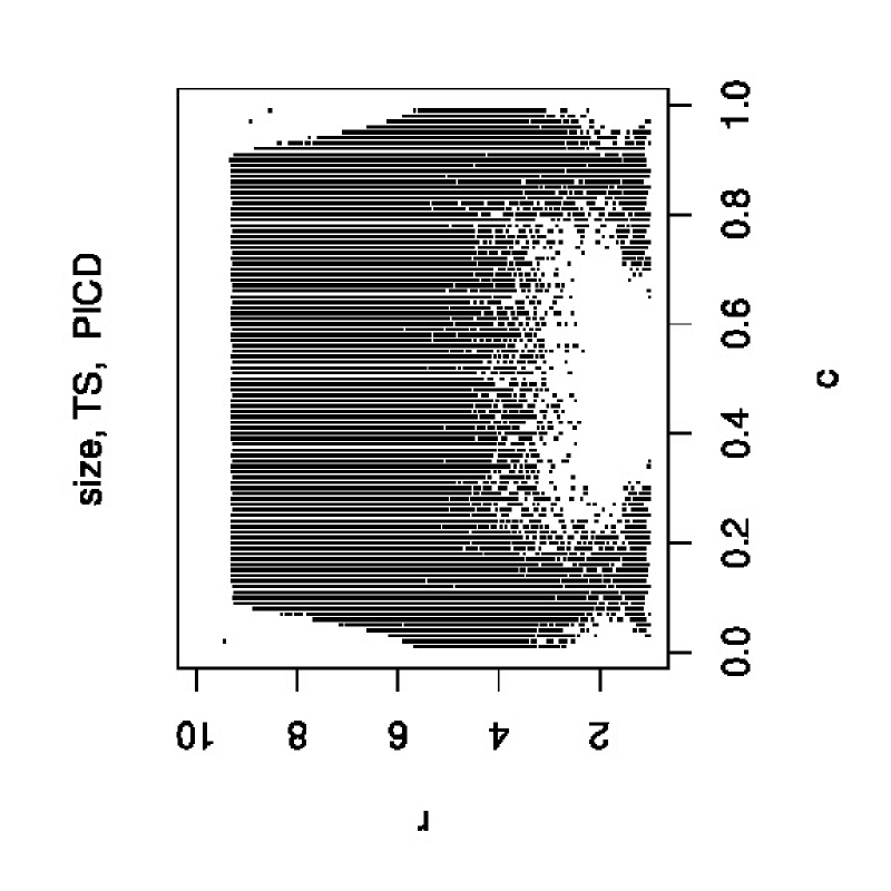
We present the empirical size estimates of the tests based on the domination number of PICD with approach (i) as two-level image plots (with empirical sizes not significantly different from 0.05 in black dots, and others are blanked out in white) with $n=20$, $c=.01,.02,\ldots,.99$ and $r=1.00,1.01,\ldots,2.10$ in Figure 4 (the plots for $n=50$ and $100$ have the similar trend, hence not presented). Notice that the sizes for the right-sided alternatives are at about the nominal level for $(r,c)$ around $(1,0)$ or $(1,1)$, while the sizes for the left-sided alternatives are about the nominal level of 0.05 at the asymptotically non-degenerate $(r,c)=(r^{*},c)$ pairs for $c\in(.25,.75)$. The reason for the asymmetric performance for the left-sided versus right-sided alternatives is that $p_{u}(r,c,n)$ values are higher (i.e., close to 1) around $(r,c)=(1,0)$ or $(1,1)$, and lower for other values, but away from 1 or 0 for $(r,c)=(r^{*},c)$ pairs. Therefore, for the power analysis, we only consider $(r,c)=(r^{*},c)$ pairs, as empirical size is closer to the nominal level for these parameters in approach (i).

In approach (ii), by construction the size estimates should be around the nominal level of .05. But due to the discrete nature of $\gamma_{n,m}$ with very few atoms for small $n$ and $m$, the exact test is liberal or conservative depending on whether we include the critical value in our size estimation. In particular, let $\gamma_{n,m,i}$ be the domination number for sample $i$ and $\gamma_{.05}$ be the 5th percentile for the exact distribution of $\gamma_{n,m}(r,c)$ (as in Theorem S6.1). Also let $\alpha_{inc}:=\sum_{i=1}^{N_{mc}}\gamma_{n,m,i}\leq\gamma_{.05}$ and $\alpha_{exc}:=\sum_{i=1}^{N_{mc}}\gamma_{n,m,i}<\gamma_{.05}$. Then for testing the left-sided alternative, $\alpha_{inc}$ tends to be much larger than .05 (implying the procedure is liberal) and $\alpha_{exc}$ tends to be much smaller than .05 (implying the procedure is conservative). In our power computations with approach (ii), we adjust for this discrepancy.

The size estimates in approach (iii) depend on the sample size $n$, and the parameters $r$ and $c$, i.e. they tend to be liberal for some values of $(r,c)$, and conservative for others, especially when $n$ is not large enough. Our simulations suggest that large sample sizes are needed (about 30 or more per each subinterval seems to work), where the required sample size would also depend on $r$ and $c$ as well. Hence we do not present approach (iii) except for the large sample simulation cases (in the cases with $n=1000$ here).

We estimate the empirical sizes of the tests based on the arc density of the PICDs and CICDs for $n=20,50$ and 100 and $c=.01,.02,\ldots,.99$ with $r=1.1,1.2,\ldots,10.0$ for PICDs and $\tau=.1,.2,\ldots,10.0$ for CICDs. For the one-sided alternatives, the regions at which size estimates are about the nominal level of 0.05 are somewhat complementary, in the sense that, the sizes are appropriate for the parameter combinations in one region for left-sided alternative and mostly in its complement for the right-sided alternative. We also observe that arc density of PICD has appropriate size for the two-sided alternative for more parameter combinations, and arc density of CICD has appropriate size for the left-sided alternative for more parameter combinations. See Figure S3 in the Supplementary Materials Section for the related image plots of the empirical size estimates.

6.2 Empirical Power Analysis

We perform a power analysis to determine which tests have better performance in detecting deviations from uniformity. For the alternatives (i.e., deviations from uniformity), we consider five types of non-uniform distributions with support in $(0,1)$:

• $f_{1}(x,\delta)=(2\delta x+1-\delta)\mathbf{I}(0<x<1)$,

• $f_{2}(x,\sigma)=\phi(x,1/2,\sigma)/(\Phi(1,1/2,\sigma)-\Phi(0,1/2,\sigma))\mathbf{I}(0<x<1)$ where $\phi(x,1/2,\sigma)$ is the pdf for normal distribution with mean $\mu=1/2$ and standard deviation $\sigma$, (i.e., normal distribution with $\mu=1/2$ restricted to $(0,1)$),

• $f_{3}(x,\delta)=(\delta\,\left(x-1/2\right)^{2}+1-\delta/12)\mathbf{I}(0<x<1)$,

• $f_{4}(x,\varepsilon)=(1/(1-2m\varepsilon))\mathbf{I}(x\in(0,1)\setminus\cup_{i=0}^{m}(i/m-\varepsilon,i/m+\varepsilon))$, that is, $f_{4}(x,\varepsilon)$ is a pdf so that $\varepsilon\times 100$ % of the regions around the $m$ subinterval end points are prohibited, and the data is uniform in the remaining regions.

• $f_{5}(x,\varepsilon^{\prime})=(1/2m\varepsilon^{\prime})\mathbf{I}(x\in(0,1)\cap(\cup_{i=0}^{m}(i/m-\varepsilon^{\prime},i/m+\varepsilon^{\prime})))$, that is, $f_{5}(x,\varepsilon^{\prime})$ is a distribution so that data is uniform over the $\varepsilon^{\prime}\times 100$ % of the regions around the $m$ subinterval end points are prohibited, and the remaining regions are prohibited. Notice that the supports of $f_{4}(x,\varepsilon)$ and $f_{5}(x,\varepsilon^{\prime})$ are complimentary in $(0,1)$.

That is,

$$H^{I}_{a}:~{}f=f_{1}(x,\delta)\text{ with }\delta\in(0,1)~{}~{}~{}H^{II}_{a}:~{}f=f_{2}(x,\sigma)\text{ with }\sigma>0~{}~{}~{}H^{III}_{a}:~{}f=f_{3}(x,\delta)\text{ with }\delta\in(0,12]\\ ~{}~{}~{}H^{IV}_{a}:~{}f=f_{4}(x,\varepsilon)\text{ with }\varepsilon\in(0,1/2)\text{ and }H^{V}_{a}:~{}f=f_{5}(x,\varepsilon^{\prime})\text{ for }\varepsilon^{\prime}\in(0,1/2)$$

In type I alternatives, $\delta=0$ corresponds to $\mathcal{U}(0,1)$ distribution, and with increasing $\delta>0$, the density of the distribution is more clustered around 1 and less clustered around 0; in type II alternatives, with decreasing $\sigma$, the density of the distribution gets more clustered around 1/2 (and less clustered around the end points, 0 and 1); and in type III alternatives, $\delta=0$ corresponds to $\mathcal{U}(0,1)$ distribution, and with increasing $\delta>0$, the density of the distribution is more clustered around the end points, 0 and 1, and less clustered around 1/2. Types IV and V alternatives are actually motivated from two-class one-dimensional spatial point patterns called segregation and association. Roughly defined, segregation is the pattern in which points from the same class tend to cluster, while under association, points from one class is clustered around the points from the other class and vice versa. In one-dimensional case, the segregation alternative is as in $H^{IV}_{a}$, where $X$ points are distributed according to $f_{4}$ and $Y$ points constitute the end points of the interval partition of $(0,1)$ (i.e., {0,1/(m-1),2/(m-1),…,1}. Hence, $X$ points tend to stay away from $Y$ points, which suggests segregation between the classes $X$ and $Y$. Furthermore, $\varepsilon=0$ in type IV alternative corresponds to the null case (i.e., uniform distribution). The association alternative is as in $H^{V}_{a}$. The pdf under type I alternative is skewed left for $\delta>0$, while pdfs under other alternatives are symmetric around 1/2. See Figure S6 in the Supplementary Materials Section for sample plots of the pdfs with various parameters for alternative types I-III.

Figure 5: Power estimates under under $H^{I}_{a}:~{}F=F_{1}(x,\delta=.8)$, $H^{II}_{a}:~{}F=F_{2}(x,\sigma=0.2)$, $H^{III}_{a}:~{}F=F_{3}(x,\delta=8)$, with $n=50$ and $N_{mc}=10000$. $G_{bin}$ and $G_{emp}$: tests based on domination number of PICD with approaches (i) and (ii), respectively, KS: Kolmogorov-Smirnov test, $\chi^{2}$: Chi-square test, NT: $T_{n}^{(2)}$ test based on the uniformity characterization, TB1 and TB2: two versions of the entropy-based tests. Tests presented in each row are indicated in the legend in that row.

Figure 6: Power estimates under under $H^{IV}_{a}:~{}F=F_{1}(x,\varepsilon)$, case (1) with $\varepsilon=.4,\,n=50,\,m=7$ and $N_{mc}=10000$ (left column), case (2) $\varepsilon=.04,\,n=1000,\,m=32$ and $N_{mc}=1000$ (middle column), and case (3) $\varepsilon=.04,\,n=1000,\,m=20$ and $N_{mc}=1000$ (right column). Labeling of the tests are as in Figure 5. Tests presented in each row are indicated in the legend in that row.

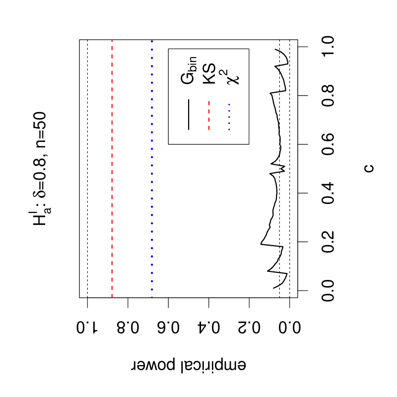
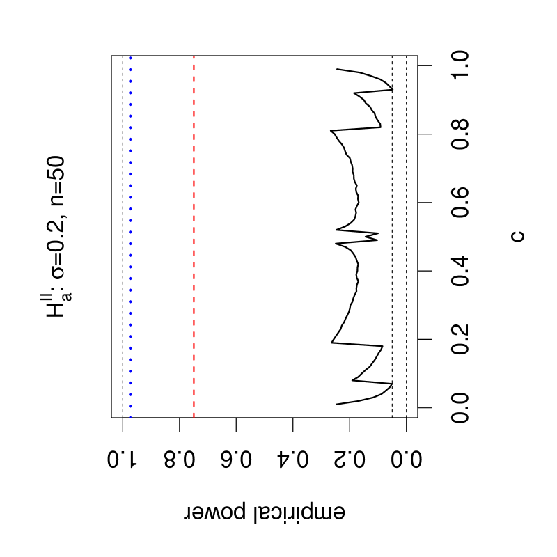
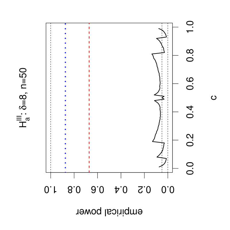
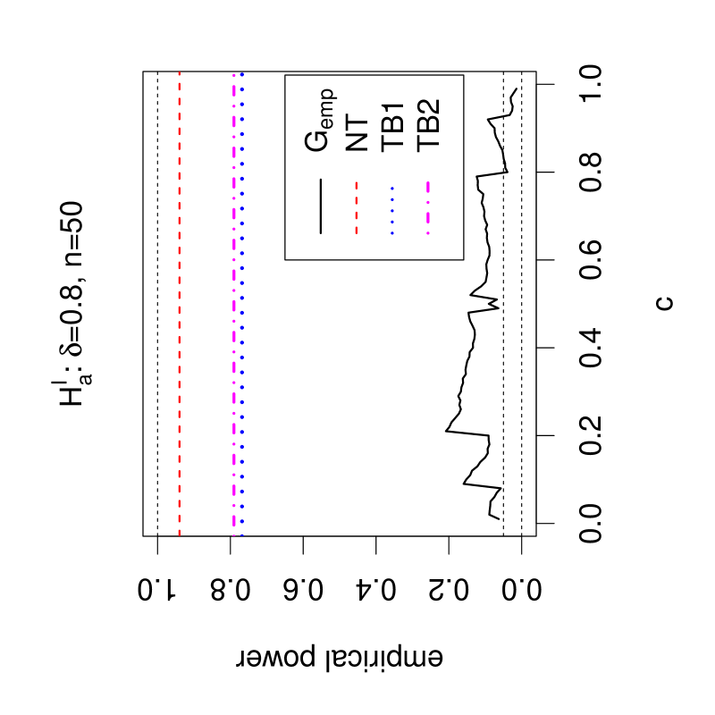
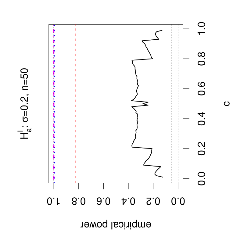
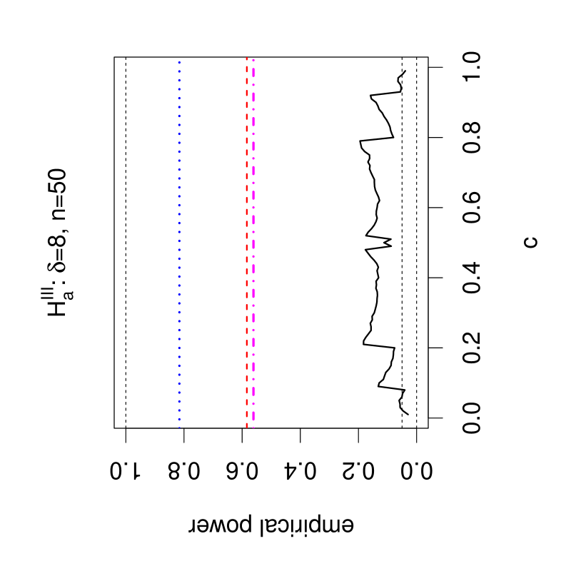
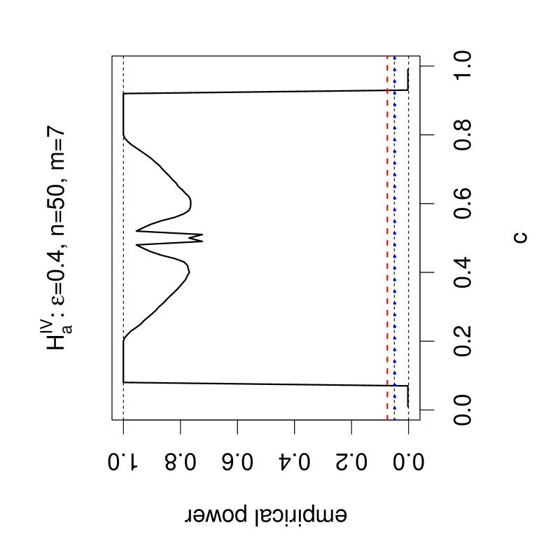
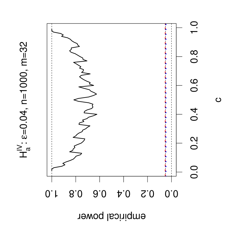
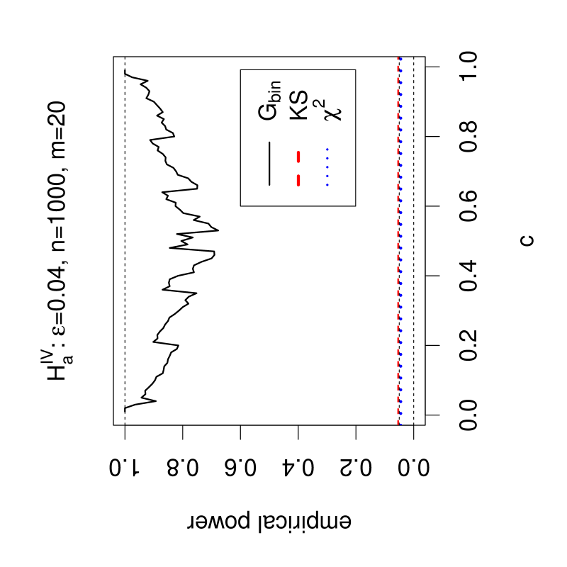
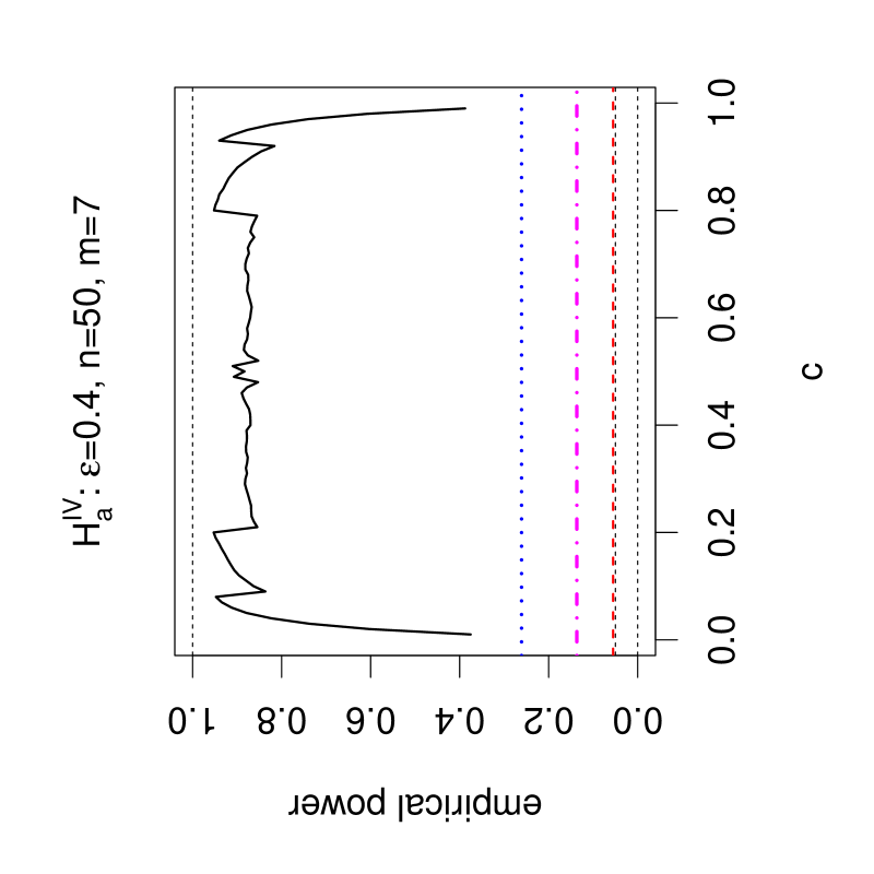
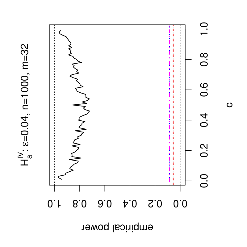
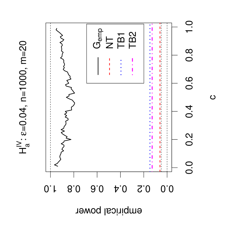
Under each alternative, we generate $n$ points according to the specified alternatives with various parameters. In particular, for $H^{I}_{a}:~{}F=F_{1}(x,\delta)$, we consider $\delta=.2,.4,.6,.8$, for $H^{II}_{a}:~{}F=F_{2}(x,\sigma)$, we consider $\sigma=.1,.2,.3,.4$, for $H^{III}_{a}:~{}F=F_{3}(x,\delta)$, we consider $\delta=2,4,6,8$, and for $H^{IV}_{a}:~{}F=F_{4}(x,\varepsilon)$, we consider $\varepsilon=.1,.2,.3,.4$ (also called $H^{IV}_{a}$-case (1)). For the domination number of PICDs, we replicate each case $N_{mc}$ times for $(r,c)=(r^{*},c)$ with $c=.01,.02.\ldots,.99$ (i.e., for $(r,c)$ values that make $\gamma_{n,2}(\mathcal{U},r,c)$ non-degenerate in the limit (see Theorem 3.4)). We compute the power using the critical values based on $\operatorname{BIN}(m,p_{u}(r,c,\lfloor{n/m}\rfloor))$ distribution (i.e., approach (i)) and based on the empirical critical values (i.e., approach (ii)). For types I-IV alternatives, we take $n=20,50,100$ and $N_{mc}=10000$. By construction, our domination number test is more sensitive for segregation/association type alternatives which also implies the same direction for each subinterval considered hence, the sum of domination number over the subintervals detects such deviations from uniformity better. In fact, we have consistency results for the domination number test under $H^{IV}_{a}$ and $H^{V}_{a}$ type alternatives (see Section 7). These consistency results suggest that domination number test gets very sensitive under very mild forms of $H^{IV}_{a}$ and $H^{V}_{a}$ when $n$ gets large. Along this line, we consider two more cases for the type IV alternative in addition to case (1). More specifically, we consider $H^{IV}_{a}$-case (1): $\varepsilon=.1,.2,.3,.4$ $n=50$, $m=7\approx\sqrt{n}$ and $N_{mc}=10000$, $H^{IV}_{a}$-case (2): $n=1000$, $m=32\approx\sqrt{n}$ and $N_{mc}=1000$; and $H^{IV}_{a}$-case (3): $n=1000$, $m=20$ and $N_{mc}=1000$ where in cases (2) and (3) we take $\varepsilon=.01,.02,.03,.04$.

For the arc density of the ICDs, we generate $n$ points according to the specified alternatives with various parameters (where $n$ is taken as in the simulations for the domination number for the null case and each alternative). With CICDs, we use $(\tau,c)$ for $\tau=.1,.2,\ldots,10.0$ and $c=.01,.02.\ldots,.99$ and with PICDs, we use $(r,c)$ for $r=1.1,1.2,\ldots,10.0$ and $c=.01,.02.\ldots,.99$. With CICDs, for each $(\tau,c)$ and $\delta$ combination, and with PICDs, for each $(r,c)$ and $\delta$ combination, we replicate the sample generation $N_{mc}$ times. We compute the power using the asymptotic critical values based on the normal approximation. We also keep the parameter combinations ($(r,c)$ for PICDs and $(\tau,c)$ for CICDs) at which the tests have the appropriate level (of .05), i.e., if the test is conservative or liberal for the one-sided version in question, we ignore that parameter combination in our power estimation, as they would yield unreliable results which might have a substantial effect on the power values. We call this procedure the “size adjustment” for power estimation. For the arc density of PICDs and CICDs, we only report the maximum power estimates under each alternative.

$H^{I}_{a}$, $n=50$
	$\delta=0.2$	$\delta=0.4$	$\delta=0.6$	$\delta=0.8$
PICD	.33	.51	.76	.94
	.15	.35	.64	.88
CICD	.19	.43	.71	.92
	.13	.33	.62	.88
$G_{bin}$	.06	.08	.09	.14
$G_{emp}$	.06	.09	.12	.21
KS	.11	.32	.62	.88
$\chi^{2}$	.07	.17	.38	.68
$T_{n}^{(2)}$	.13	.37	.70	.94
TB1	.08	.20	.43	.77
TB2	.08	.20	.43	.79

$H^{II}_{a}$, $n=50$
	$\sigma=0.1$	$\sigma=0.2$	$\sigma=0.3$	$\sigma=0.4$
PICD	1.00	1.00	.79	.39
	1.00	1.00	.79	.37
CICD	1.00	1.00	.81	.42
	1.00	1.00	.81	.41
$G_{bin}$	.99	.25	.07	.06
$G_{emp}$	.95	.37	.11	.07
KS	1.00	.75	.17	.07
$\chi^{2}$	1.00	.97	.39	.14
$T_{n}^{(2)}$	1.00	.83	.17	.07
TB1	1.00	.99	.54	.22
TB2	1.00	1.00	.68	.31

$H^{III}_{a}$, $n=50$
	$\delta=2$	$\delta=4$	$\delta=6$	$\delta=8$
PICD	.41	.66	.92	.99
	.28	.66	.92	.99
CICD	.19	.53	.86	.98
	.19	.52	.86	.98
$G_{bin}$	.07	.07	.09	.14
$G_{emp}$	.06	.07	.11	.19
KS	.09	.19	.40	.67
$\chi^{2}$	.09	.27	.38	.87
$T_{n}^{(2)}$	.07	.14	.31	.58
TB1	.07	.19	.48	.82
TB2	.03	.06	.21	.56

$H^{IV}_{a}$, $n=50$
	$\varepsilon=0.1$	$\varepsilon=0.2$	$\varepsilon=0.3$	$\varepsilon=0.4$
PICD	.27	.27	.34	.50
	.06	.08	.10	.14
CICD	.11	.15	.28	.52
	.06	.07	.08	.24
$G_{bin}$	.28	1.00	1.00	1.00
$G_{emp}$	.88	.95	.95	.95
KS	.05	.06	.06	.07
$\chi^{2}$	.05	.05	.05	.05
$T_{n}^{(2)}$	.05	.05	.05	.06
TB1	.07	.10	.15	.26
TB2	.06	.07	.09	.14

Table 1: The power estimates under the alternatives $H_{a}^{I}$ to $H_{a}^{IV}$ with all four parameter values considered and $n=50$ and $N_{mc}=10000$ for the tests we employed. PICD and CICD represent the arc densities of the ICD tests, and for each, top row is without size adjustment and bottom row is with size adjustment (see the text for the description of size adjustment), $G_{bin}$ and $G_{emp}$: tests based on domination number of PICD with approaches (i) and (ii), KS: Kolmogorov-Smirnov test, $\chi^{2}$: Chi-square test, NT: $T_{n}^{(2)}$ test based on the uniformity characterization, TB1 and TB2: two versions of the entropy-based tests.

$H^{IV}_{a}$, $n=1000$, $m=32$, $N_{mc}=1000$
	$\varepsilon=0.01$	$\varepsilon=0.02$	$\varepsilon=0.03$	$\varepsilon=0.04$
PICD	.08	.08	.08	.08
	.08	.08	.08	.08
CICD	.08	.08	.08	.08
	.07	.08	.08	.08
DN	.49	1.00	1.00	1.00
	.66	.95	.96	.97
KS	.04	.04	.04	.05
$\chi^{2}$	.05	.05	.06	.05
$T_{n}^{(2)}$	.04	.04	.04	.06
TB1	.04	.07	.08	.09
TB2	.04	.06	.07	.09

$H^{IV}_{a}$, $n=1000$, $m=20$, $N_{mc}=1000$
	$\varepsilon=0.01$	$\varepsilon=0.02$	$\varepsilon=0.03$	$\varepsilon=0.04$
PICD	.08	.08	.08	.08
	.08	.08	.08	.08
CICD	.08	.08	.08	.07
	.08	.08	.08	.07
$G_{bin}$	.40	1.00	1.00	1.00
$G_{emp}$	.61	.95	.95	.97
KS	.06	.04	.05	.05
$\chi^{2}$	.05	.05	.04	.05
$T_{n}^{(2)}$	.06	.05	.05	.06
TB1	.04	.08	.09	.15
TB2	.04	.07	.09	.13

Table 2: The power estimates under the alternatives $H_{a}^{IV}$ with all four $\varepsilon$ values considered and $n=1000$ and $N_{mc}=1000$ for the tests we employed. Labeling of the tests is as in Table 1.

The power comparisons between PICD domination number test, KS, $\chi^{2}$, TB1, TB2 and $T_{n}^{(2)}$ tests are presented in Figure 5 for alternatives $H_{a}^{I}-H_{a}^{III}$, and in Figure 6 for alternatives $H_{a}^{IV}$-cases (1)-(3). The power estimates based on asymptotic critical values of the tests (i.e., the power estimates for the test based on domination number of PICD with approach (i), Kolmogorov-Smirnov test, and Chi-square test) are provided in the top row and those based on Monte Carlo critical values (for the test based on domination number of PICD with approach (ii), $T_{n}^{(2)}$ test based on the uniformity characterization, two versions of the entropy-based tests) are provided in the bottom row in these figures. The power estimates under alternatives $H_{a}^{I}-H_{a}^{III}$ and $H_{a}^{IV}$-case(1) are presented in Table 1, and those under alternative $H_{a}^{IV}$-cases (2) and (3) in Table 2; in both tables the power estimates are rounded to two decimal places. In Figures 5 and 6, we do not present the power estimates for ICD arc density tests, due to the difficulty in presentation since ICD arc density tests depend on two parameters. For the domination number test, the power estimates based on asymptotic critical values are provided in the top row and those based on Monte Carlo critical values are provided in the bottom row in these figures. In Tables 1 and 2, we only present the maximum power estimates for the ICD arc density tests for the two-sided alternative and for the CICD domination number tests. Considering Figures 5 and 6 and Tables 1 and 2, we observe that power estimates increase as the departure from uniformity gets more severe. In particular, power estimate increases as $\delta$ increases in $H_{a}^{I}$ or $H_{a}^{II}$, as $\varepsilon$ increases in $H_{a}^{IV}$ and as $\sigma$ decreases in $H_{a}^{II}$. Under $H_{a}^{I}-H_{a}^{III}$ and $H_{a}^{IV}$-case(1), arc density of PICD and CICD has the highest power estimates, where PICD arc density tends to perform better (worse) than CICD arc density under $H_{a}^{I}-H_{a}^{III}$ (under $H_{a}^{IV}$-case (1)). Under $H_{a}^{I}$, ICD arc density tests are followed by $T_{n}^{(2)}$; under $H_{a}^{II}$, ICD arc density tests are followed by TB1 and TB2; under $H_{a}^{III}$, ICD arc density tests are followed by $\chi^{2}$ test; and under $H_{a}^{IV}$-case (1), ICD domination number test is followed by CICD arc density test. Under $H_{a}^{IV}$-cases (2) and (3) ICD domination number tests have the highest power estimates, where under case (1) PICD domination number test with approach (i) and under case (2) domination number test with approach (ii) has better performance, and power estimates for the other tests are just above .05 or at about .05. In these large sample cases, approach (iii) also works, and has higher power estimates than the other two approaches (corresponding estimates not presented to be consistent with the presentations of the other alternatives). Moreover, PICD domination number test performs better when the support is partitioned by $m\approx\sqrt{n}$. We omit the power performance under $H^{V}_{a}$ as it is the opposite pattern to the one under $H^{IV}_{a}$. More simulation results for the arc density of ICDs are presented in in the Supplementary Materials Section, where we observe that the power estimates are symmetric around $c=1/2$ under types II-IV alternatives, which is in agreement with the symmetry in the corresponding pdfs (around $c=1/2$).

We also considered the power comparisons under $H_{a}^{I}-H_{a}^{III}$ and $H_{a}^{IV}$ case (1) at the same alternative parameters with $n=N_{mc}=1000$, to see the effect of the large samples on the power estimates. The results are similar to those in the smaller sample cases, with higher power for each test (hence not presented). In particular, under $H_{a}^{I}-H_{a}^{III}$ all tests have much higher power, with most having power virtually 1.00, but domination number tests with approaches (i) and (ii) exhibit mild improvement, while under $H_{a}^{IV}$ case (1), PICD domination number tests attain the highest power estimates, virtually 1.00, while there is mild improvement in the performance of other tests, except for TB1 and TB2, which show moderate improvement. We also observe that in the large sample case, PICD domination number with approach (iii) attains very high power under each alternative.

The above methodology can easily be extended for testing non-uniform distributions (see Remark S6.4 in the Supplementary Materials Section).

7 Consistency of the Tests based on Domination Number of PICDs under $H_{a}^{IV}$ and $H_{a}^{V}$

Let $b_{\alpha}$ be the $\alpha\times 100$th percentile of the binomial distribution $\operatorname{BIN}(m,p_{u}(r,c,\lfloor{n/m}\rfloor))$.

Theorem 7.1.

(Consistency - Type I) Let $\gamma_{n,m}(F,r,c)$ be the domination number under segregation and association alternatives, $H^{IV}_{a}$ and $H^{V}_{a}$, respectively, in the multiple interval case with $m$ intervals. The test against segregation with $F=F_{4}(x,\varepsilon)$ which rejects for $G_{n}<b_{\alpha}$ and the test against association with $F=F_{5}(x,\varepsilon^{\prime})$ which rejects for $G_{n}>b_{1-\alpha}$ are consistent.

Proof: Given $F=F_{4}(x,\varepsilon)$. Let $\gamma_{n,m}(\mathcal{U},r,c)$ be the domination number for $\mathcal{X}_{n}$ being a random sample from $\mathcal{U}(0,1)$. Then $P(\gamma_{n,m}(F,r,c)=1)\geq P(\gamma_{n,m}(\mathcal{U},r,c)=1)$; and $P(\gamma_{n,m}(F,r,c)=2)\leq P(\gamma_{n,m}(\mathcal{U},r,c)=2)$. Hence $G_{n}<mp_{u}(r,c,\lfloor{n/m}\rfloor)$ with probability 1, as $n\gg m\rightarrow\infty$. Furthermore, $\operatorname{BIN}(m,p_{u}(r,c,\lfloor{n/m}\rfloor))$ distribution converges to normal distribution with mean $mp_{u}(r,c,\lfloor{n/m}\rfloor)$ and variance $mp_{u}(r,c,\lfloor{n/m}\rfloor)(1-p_{u}(r,c,\lfloor{n/m}\rfloor))$. Hence consistency follows from the consistency of tests which have asymptotic normality. The consistency against the association alternative can be proved similarly. $\blacksquare$

Below we provide a result which is stronger, in the sense that it will hold for finite $m$ as $n\rightarrow\infty$. Let $\overline{G}_{n}:=G_{n}/m$ (i.e., domination number averaged over the number of subintervals) and $z_{\alpha}$ be the $\alpha\times 100$-th percentile of the standard normal distribution.

Theorem 7.2.

(Consistency - Type II) Let $\gamma_{n,m}(F,r,c)$ be the domination numbers under segregation and association alternatives $H^{IV}_{a}$ and $H^{V}_{a}$, respectively, in the multiple interval case with $m$ intervals where $m<\infty$ is fixed. Let $m^{*}(\alpha,\varepsilon):=\left\lceil\Bigl{(}\frac{\sigma\cdot z_{\alpha}}{\overline{G}_{n}(r,c)-\mu}\Bigr{)}^{2}\right\rceil$ where $\lceil\cdot\rceil$ is the ceiling function and $\varepsilon$-dependence is through $\overline{G}_{n,m}(r,c)$ under a given alternative. Then the test against $H^{IV}_{a}$ which rejects for $S_{n,m}<z_{\alpha}$ is consistent for all $\varepsilon\in\left(0,\min(c,1-c)\right)$ and $m\geq m^{*}(\alpha,\varepsilon)$, and the test against $H^{V}_{a}$ which rejects for $S_{n,m}>z_{1-\alpha}$ is consistent for all $\varepsilon\in\left(0,\min(c,1-c)\right)$ and $m\geq m^{*}(1-\alpha,\varepsilon)$.

Proof: Let $\varepsilon\in\left(0,\min(c,1-c)\right)$. Under $H^{IV}_{a}$, $\gamma_{n}(F,r,c)$ is degenerate in the limit as $n\rightarrow\infty$, which implies $\overline{G}_{n}(r,c)$ is a constant a.s. In particular, for $\varepsilon\in\left(0,\min(c,1-c)\right)$, $\overline{G}_{n}(r,c)=1$ a.s. as $n\rightarrow\infty$. Then the test statistic $S_{n,m}=\sqrt{m}(\overline{G}_{n}(r,c)-\mu)/\sigma$ is a constant a.s. and $m\geq m^{*}(\alpha,\varepsilon)$ implies that $S_{n,m}<z_{\alpha}$ a.s. Furthermore, $S_{n,m}\stackrel{{\scriptstyle\mathcal{L}}}{{\rightarrow}}N(0,1)$ as $n\to\infty$. Hence consistency follows for segregation.

Under $H^{V}_{a}$, as $n\rightarrow\infty$, $\overline{G}_{n}(r,c)=2$ for all $\varepsilon\in\left(0,\min(c,1-c)\right)$ a.s. Then $m\geq m^{*}(1-\alpha,\varepsilon)$ implies that $S_{n,m}>z_{1-\alpha}$ a.s., hence consistency follows for association. $\blacksquare$

Notice that in Theorem 7.2 we actually have more than what consistency requires. In particular, we show that the power of the test reaches 1 for $m$ greater than a threshold as $n\rightarrow\infty$.

8 Discussion and Conclusions

In this article, we derive the distribution of the domination number of a random digraph family called parameterized interval catch digraph (PICD) which is based on two classes of points, say $\mathcal{X}$ and $\mathcal{Y}$. Points from one of the classes (say, class $\mathcal{X}$), denoted $\mathcal{X}_{n}$, constitute the vertices of the PICDs, while the points from the other class (say, class $\mathcal{Y}$), denoted $\mathcal{Y}_{m}$, are used in the binary relation that assigns the arcs of the PICDs. Our PICD is based on a parameterized proximity map which has an expansion parameter $r$ and a centrality parameter $c$. We provide the exact and asymptotic distributions of the domination number of the PICDs for uniform data and compute the asymptotic distribution for non-uniform data for the entire range of $(r,c)$.

We demonstrate an interesting behavior of the domination number of the PICD for one-dimensional data. For uniform data or data from a distribution which satisfies some regularity conditions and fixed finite sample size $n>1$, the distribution of the domination number restricted to any interval is a translated form of Bernoulli distribution, $\operatorname{BER}(p)$, where $p$ is the probability that the domination number being 2. In the case of $\mathcal{Y}_{2}=\{y_{1},y_{2}\}$ with $\mathcal{U}(y_{1},y_{2})$ data, for finite $n\geq 1$, the parameter of the asymptotic distribution of the domination number of the PICD based on uniform data (i.e. probability of domination number being 2, denoted $p_{u}(r,c)$) is continuous in $r$ and $c$ for all $r\geq 1$ and $c\in(0,1)$. For fixed $(r,c)\in[1,\infty)\times(0,1)$, $p_{u}(r,c)$ exhibits some discontinuities. The asymptotic distribution of the domination number is degenerate for the expansion parameter $r>2$ regardless of the value of $c$. For $c\in(0,1)$ the asymptotic distribution is nondegenerate when the expansion parameter $r$ equals $r^{*}=1/\max(c,1-c)$. For $r=r^{*}$, the asymptotic distribution of the domination number is a translated form of $\operatorname{BER}(p_{u}(r^{*},c))$ where $p_{u}(r^{*},c)$ is continuous in $c$. For $r>r^{*}$ the domination number converges in probability to 1, and for $r<r^{*}$ the domination number converges in probability to 2. On the other hand, at $(r,c)=(2,1/2)$, the asymptotic distribution is again a translated form of $\operatorname{BER}(p_{u}(2,1/2))$, but there is yet another jump at $(r,c)=(2,1/2)$, as $p_{u}(2,1/2)=4/9$ while $\lim_{(r,c)\rightarrow(2,1/2)}p_{u}(r^{*},c)=2/3$. This second jump is due to the symmetry for the domination number at $c=1/2$ (see the discussion at the end of Section 3.1.1).

We employ domination number for testing uniformity of one-dimensional data. In this application, we have $n$ $\mathcal{X}$ points and we take $m$ $\mathcal{Y}$ points to be the equidistant points in the support of $\mathcal{X}$ points. For example, if the support of $\mathcal{X}$ points is $(0,1)$, we take $\mathcal{Y}$ points to be $\mathcal{Y}_{m}=\{0,1/(m-1),2/(m-1),\ldots,1\}$. Since under $H_{o}$, $H^{IV}_{a}$ and $H^{V}_{a}$ the data is uniform with different support regions, we can extend the methodology to the random $\mathcal{Y}_{m}$ case, but currently the method is only applicable given $\mathcal{Y}_{m}$ as above.

We compare the size and power performance of PICD domination number with two well known tests, namely, Kolmogorov-Smirnov (KS) test and Pearson’s $\chi^{2}$ goodness-of-fit test, three recently introduced tests, the uniformity test based on Too-Lin characterization, denoted as $T_{n}^{(2)}$ (Milošević,, 2018), and two entropy-based tests, denoted as TB1 and TB2 in (Zamanzade,, 2015), and also the arc density of PICDs and of another ICD family called central ICD (CICD), by Monte Carlo simulations. Based on the simulation results, we see that ICDs have better performance than their competitors (in terms of size and power). Arc density of ICDs perform better than others under most alternatives for some of the parameter values and the domination number outperforms others under certain types of alternatives. In particular, under the alternatives $H_{a}^{I}-H_{a}^{III}$, ICD arc density tests outperform other tests, and under $H_{a}^{IV}$-cases (1)-(3), PICD domination number tests outperform other tests. For the ICD arc density tests, we use the asymptotic critical values based on normal approximation. For the PICD domination number test, we use the binomial critical values with an approximate probability of success (i.e., approach (i)) and also the empirical critical values based on Monte Carlo simulations (i.e., approach (ii)). For $T_{n}^{(2)}$, TB1 and TB2 tests, the critical values are also based on Monte Carlo simulations.

We recommend using the PICD domination number test for uniformity in the following scenario. If we are testing uniformity of data in multiple intervals (by hypothesis or one can partition the support of the data), and the deviation from uniformity is in the same direction at each interval, then, by construction, domination number tends to be more sensitive to detect such alternatives (even if they are very mild deviations from uniformity). Among the types of critical value computations, we recommend the use of the exact distribution provided in Theorem S6.1 (with Monte Carlo critical values as an approximation in practice), i.e., approach (ii) for small samples (this approach could be used provided running time is feasible), and the approximate Binomial test for any $n$, i.e., approach (i) (see Section 6.1). For large samples, binomial test with asymptotic probability of success (i.e., approach (iii)) could also be employed. Our simulations suggest that about 30 or more for each subinterval seems to work for most $(r^{*},c)$ combination, however, the sample size requirements for approach (iii) have not been studied thoroughly in this article. The relevant functions for these tests are PEdom1D and TSDomPEBin1D which are available in the R package pcds which is available on github and can be installed using the command devtools::install_github("elvanceyhan/pcds") in an R session. The function PEdom1D computes the domination number when one or two one-dimensional data sets are provided, and the function TSDomPEBin1D uses the finite sample binomial approximation (i.e. approach (i)) by default or can use the asymptotic binomial version (i.e., approach (iii)) for very large samples when asy.bin=TRUE option is employed. Monte Carlo critical values can also be computed using PEdom1D with sampling from the uniform distribution of the data sets (i.e., approach (ii)). See the help pages for PEdom1D and TSDomPEBin1D for more details. The domination number approach is easily adaptable to testing nonuniform distributions as well (see Remark S6.4 for more detail). PICDs have other applications, e.g., as in Ceyhan and Priebe, (2005), we can use the domination number in testing one-dimensional spatial point patterns and our results can help make the power comparisons possible for a large family of distributions (see, e.g., Section 6.2 for a brief treatment of this issue). PICDs can also be employed in pattern classification as well (see, e.g., Priebe et al., (2003) and Manukyan and Ceyhan, (2016)). Furthermore, this article may form the foundation of the generalizations and calculations for uniform and non-uniform distributions in multiple dimensions.

In our calculations, we extensively make use of the ordering of points in $\mathbb{R}$. The order statistics of $\mathcal{Y}_{m}$ partition the support of $X$ points into disjoint intervals. This nice structure in $\mathbb{R}$ allows us to find a minimum dominating set and hence the domination number, both in polynomial time. Furthermore, the components of the digraph restricted to intervals (see Section 2.3) are not connected to each other, since the defining proximity regions $N(x_{i},r,M)\cap N(x_{j},r,M)=\emptyset$ for $x_{i},\,x_{j}$ in distinct intervals. Extension of this approach to higher dimensions is a challenging problem, since there is no such ordering for point in $\mathbb{R}^{d}$ with $d>1$. However, we can use the Delaunay tessellation based on $\mathcal{Y}_{m}$ to partition the space as in Ceyhan and Priebe, (2005). Furthermore, for most of the article and for all non-trivial results (i.e., for the exact and asymptotic distributions of the domination number), we assumed $\mathcal{Y}_{m}$ is given; removing the conditioning on $\mathcal{Y}_{m}$ is a topic of ongoing research along various directions, namely: (i) $X$ and $Y$ both have uniform distribution, (ii) $X$ and $Y$ both have the same (absolutely) continuous distribution, and (iii) $X$ is distributed as $F_{X}$ and $Y$ is distributed as $F_{Y}$ (where $F_{X}\neq F_{Y}$ and both $F_{X}$ and $F_{Y}$ are absolutely continuous).

SUPPLEMENTARY MATERIALS

S2 Additional and Illustrative Figures

S2.1 Empirical Size and Power Plots

Figure S1: Image plots for the empirical size estimates for approach (i) based on $n=50$ and $N_{mc}=10000$ for $r=1.01,1.02,\ldots,2.10$ and $c=.01,.02,\ldots,.99$ for the two-sided, right-sided and left-sided alternatives (left to right). The size estimates are coded in gray-level (as size increases the gray level gets darker).

Figure S2: Image plots for the empirical size estimates for approach (i) based on $n=20$ (top row) $n=50$ (middle row) and $n=100$ (bottom row) and $N_{mc}=10000$ for $r=1.01,1.02,\ldots,2.10$ and $c=.01,.02,\ldots,.99$ for the two-sided, right-sided and left-sided alternatives (left to right). The size estimates significantly different from .05 are blanked out, while size estimates within .0536 and .0464 are plotted in black. The solid lines indicates the case of $(r,c)$ (i.e., $(r,c)=(r^{*},c)$) which yields the asymptotically non-degenerate distribution for the domination number.

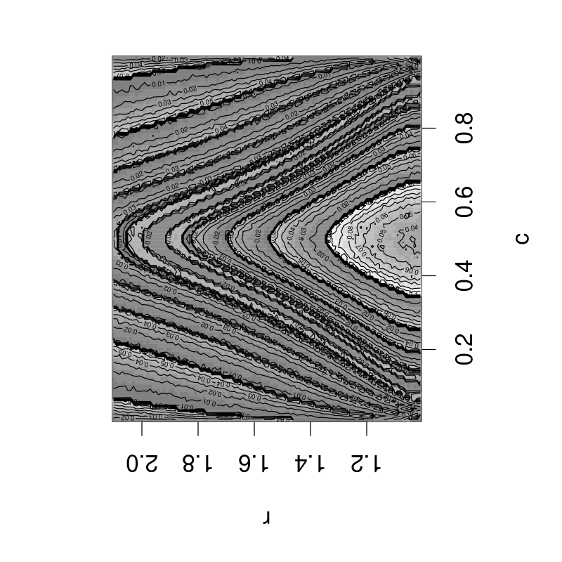
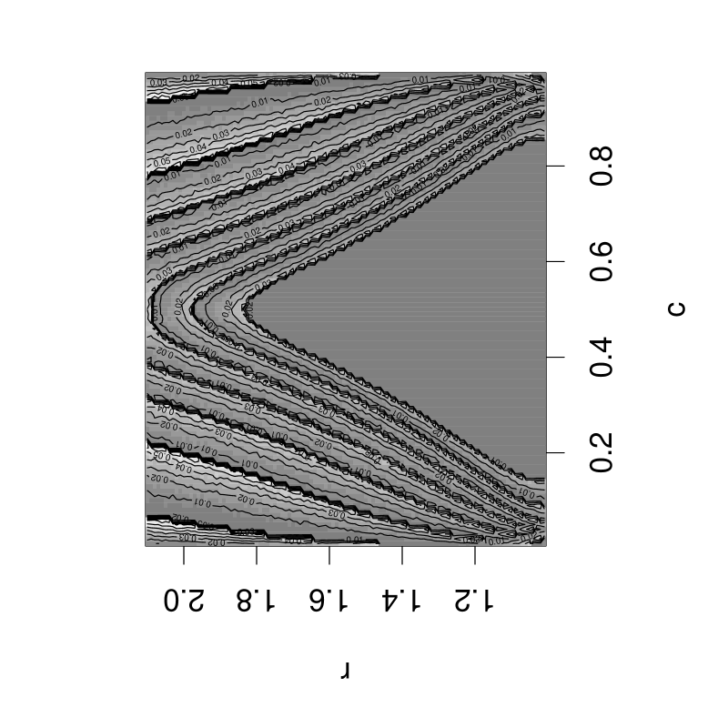
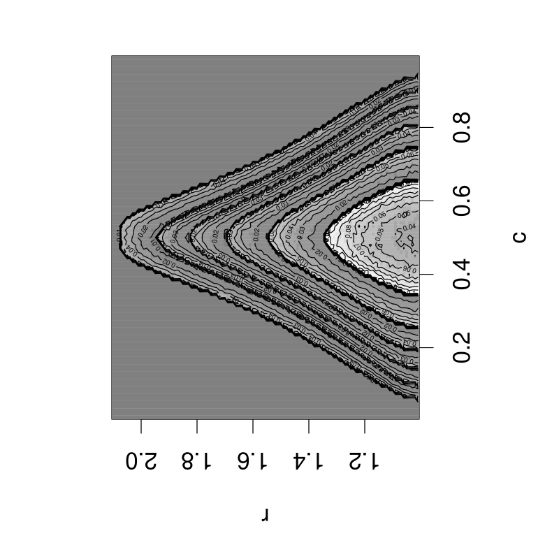
We present the empirical size estimates of the tests based on the domination number of PICD with approach (i) as gray-scale image plots for the two-sided, right- and left-sided alternatives with $n=50$, $c=.01,.02,\ldots,.99$ and $r=1.01,\ldots,2.10$ in Figure S1 (the plots for $n=20$ and $n=100$ have the similar trend, hence not presented). A similar version of these plots are the image plots in S2 for the empirical size estimates for approach (i) based on $n=20$ (top row) 50 (middle row) and 100 (bottom row) and $N_{mc}=10000$ for $r=1.01,1.02,\ldots,2.10$ and $c=.01,.02,\ldots,.99$ for the two-sided, right-sided and left-sided alternatives (left to right). The size estimates significantly different from .05 are blanked out, while size estimates within .0536 and .0464 are plotted in black. The solid lines indicates the case of $(r,c)$ (i.e., $(r,c)=(r^{*},c)$) which yields the asymptotically non-degenerate distribution for the domination number. Notice that there is symmetry in size estimates around $c=1/2$.

We present the empirical size estimates of the tests based on the arc density of the ICDs in two-level image plots (with empirical sizes not significantly different from 0.05 in black, and others blanked out in white) for the two-sided, right-sided and left-sided alternatives in Figure S3. The size estimates for PICDs with $n=20$, $c=.01,.02,\ldots,.99$ and $r=1.01,1.02,\ldots,10.00$ are plotted in the top row and those for CICDs with $n=20$, $c=.01,.02,\ldots,.99$ and $\tau=.01,.02,\ldots,10.00$ are plotted in bottom row. The size estimates for $n=50$ and $100$ have similar trends with sizes closer to nominal level for more parameter combinations (hence not presented). Notice the symmetry in size estimates around $c=1/2$.

Figure S3: Two-level (i.e., black and white) image plots for the empirical size estimates for the arc density of CICD and PICD based on $n=20$ and $N_{mc}=10000$ the two-sided (TS), right-sided (RS) and left-sided (LS) alternatives. The empirical sizes not significantly different from 0.05 are represented with black dots, and others are blanked out (i.e., represented with white dots). For CICD, we use $\tau=.01,.02,\ldots,10.00$ and for PICD , we use $r=1.01,1.02,\ldots,10.00$ and for both ICDs, we take $c=.01,.02,\ldots,.99$ with $N_{mc}=10000$ Monte Carlo replications.

S2.2 Illustrative Figures

Figure S4: The arcs for the PICD with $\mathcal{X}_{40}$ and $\mathcal{Y}_{10}$ both of which are uniformly generated in $(0,10)$. The parameters are provided at the top of each plot, $\mathcal{Y}$ points are represented with solid vertical lines, and the center values are represented with dotted vertical lines. Arcs are plotted at jittered locations along the $y$-axis for better visualization.

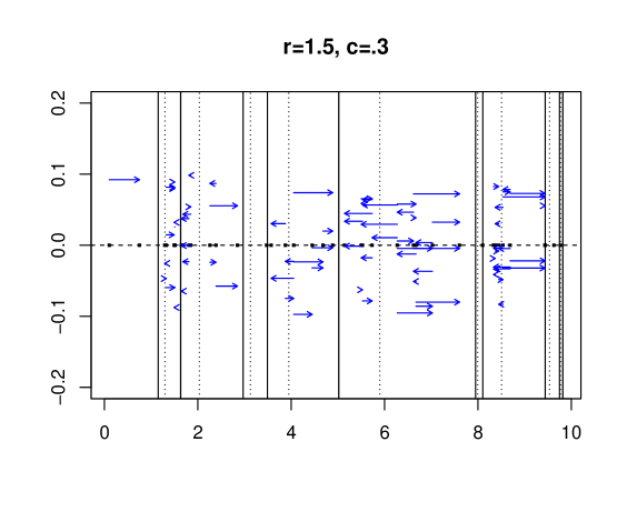
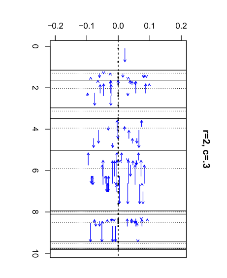
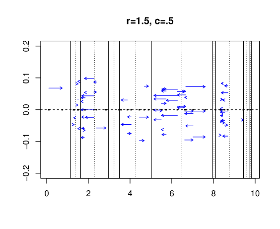
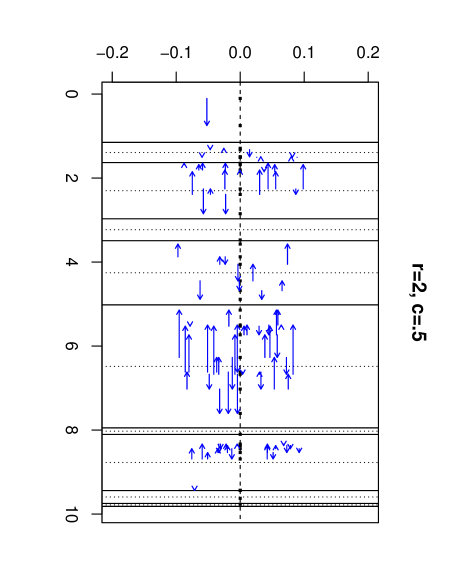
See Figure S4 for the arcs of our PICD with $\mathcal{X}_{40}$ and $\mathcal{Y}_{10}$ uniformly generated in $(0,10)$ and $(r,c)=(1.5,.3)$, $(r,c)=(2,.3)$, $(r,c)=(1.5,.5)$ and $(r,c)=(2,.5)$. This yields a disconnected digraph with subdigraphs each of which might be null or itself disconnected. (see, e.g., Figure S4 for an illustration).

We present sample plots for $\pi_{a,4}(r,c,n)$ and $\pi_{b,3}(r,c,n)$ for specific $r$ and $c$ values as a function of $n$. As $n$ increases, $\pi_{a,4}(r,c,n)$ strictly increases towards 1 (see Figure S5 (left)), and $\pi_{b,3}(r,c,n)$ decreases (strictly decreases for $n\geq 3$) towards 0 (see Figure S5 (right)).

Figure S5: The plots of probabilities $\pi_{a,4}(r=1.2,c=0.4,n)$ (left) and $\pi_{b,3}(r=2,c=0.3,n)$ (right) as a function of number of $\mathcal{X}$ points, $n$, in Main Result 1.

For the alternatives (i.e., deviations from uniformity), we consider five families of non-uniform distributions with support in $(0,1)$:

• $F_{1}(x,\delta)=(\delta x^{2}-\delta x+x)\mathbf{I}(0<x<1)+\mathbf{I}(x\geq 1)$,

• $F_{2}(x,\sigma)=(\Phi(x,1/2,\sigma)-\Phi(0,1/2,\sigma))/(\Phi(1,1/2,\sigma)-\Phi(0,1/2,\sigma))\mathbf{I}(0<x<1)+\mathbf{I}(x\geq 1)$ where $\Phi(x,1/2,\sigma)$ is the normal distribution function with mean $\mu=1/2$ and standard deviation $\sigma$, (i.e., normal distribution with $\mu=1/2$ restricted to $(0,1)$),

• $F_{3}(x,\delta)=(\delta x^{3}/3-\delta x^{2}/2+x+\delta x/6)\mathbf{I}(0<x<1)+\mathbf{I}(x\geq 1)$,

• $F_{4}(x,\varepsilon)$ is a distribution so that $\varepsilon\times 100$ % of the regions around the $m$ subinterval end points are prohibited, and the data is uniform in the remaining regions.

• $F_{5}(x,\varepsilon^{\prime})$ is a distribution so that data is uniform over the $\varepsilon^{\prime}\times 100$ % of the regions around the $m$ subinterval end points are prohibited, and the remaining regions are prohibited. Notice that the supports of $F_{4}(x)$ and $F_{5}(x)$ are complimentary in $(0,1)$.

That is,

$$H^{I}_{a}:~{}F=F_{1}(x,\delta)\text{ with }\delta\in(0,1)~{}~{}~{}H^{II}_{a}:~{}F=F_{2}(x,\sigma)\text{ with }\sigma>0~{}~{}~{}H^{III}_{a}:~{}F=F_{3}(x,\delta)\text{ with }\delta\in(0,12]\\ ~{}~{}~{}H^{IV}_{a}:~{}F=F_{4}(x,\varepsilon)\text{ with }\varepsilon\in(0,1/2)\text{ and }H^{V}_{a}:~{}F=F_{5}(x,\varepsilon^{\prime})\text{ for }\varepsilon^{\prime}\in(0,1/2)$$

\psfrag{f(x)}[cc][0.8][0]{\put(-7.5,0.0){\huge{$f_{1}(x)$}}}\psfrag{x}{\huge{$x$}}\psfrag{k=1}{\huge{$\delta=.2$}}\psfrag{k=2}{\huge{$\delta=.4$}}\psfrag{k=3}{\huge{$\delta=.6$}}\psfrag{k=4}{\huge{$\delta=.8$}}\includegraphics{TypeIAlt.ps}

\psfrag{f(x)}[cc][0.8][0]{\put(-7.5,0.0){\huge{$f_{1}(x)$}}}\psfrag{x}{\huge{$x$}}\psfrag{k=1}{\huge{$\delta=.2$}}\psfrag{k=2}{\huge{$\delta=.4$}}\psfrag{k=3}{\huge{$\delta=.6$}}\psfrag{k=4}{\huge{$\delta=.8$}}\psfrag{f(x)}[cc][0.8][0]{\put(-7.5,0.0){\huge{$f_{2}(x)$}}}\psfrag{k=1}{\huge{$\sigma=.1$}}\psfrag{k=2}{\huge{$\sigma=.2$}}\psfrag{k=3}{\huge{$\sigma=.3$}}\psfrag{k=4}{\huge{$\sigma=.4$}}\includegraphics{TypeIIAlt.ps}

\psfrag{f(x)}[cc][0.8][0]{\put(-7.5,0.0){\huge{$f_{1}(x)$}}}\psfrag{x}{\huge{$x$}}\psfrag{k=1}{\huge{$\delta=.2$}}\psfrag{k=2}{\huge{$\delta=.4$}}\psfrag{k=3}{\huge{$\delta=.6$}}\psfrag{k=4}{\huge{$\delta=.8$}}\psfrag{f(x)}[cc][0.8][0]{\put(-7.5,0.0){\huge{$f_{2}(x)$}}}\psfrag{k=1}{\huge{$\sigma=.1$}}\psfrag{k=2}{\huge{$\sigma=.2$}}\psfrag{k=3}{\huge{$\sigma=.3$}}\psfrag{k=4}{\huge{$\sigma=.4$}}\psfrag{f(x)}[cc][0.8][0]{\put(-7.5,0.0){\huge{$f_{3}(x)$}}}\psfrag{k=1}{\huge{$\delta=2$}}\psfrag{k=2}{\huge{$\delta=4$}}\psfrag{k=3}{\huge{$\delta=6$}}\psfrag{k=4}{\huge{$\delta=8$}}\includegraphics{TypeIIIAlt.ps}

Figure S6: Sample plots for the pdfs of the alternative types I (left), II (middle), and III (right). We plot pdfs for type I with $\delta=.2,.4,.6,.8$, for type II with $\sigma=.1,.2,.3,.4$, and for type III with $\delta=2,4,6,8$. The horizontal line at $1$ indicates the pdf for $\mathcal{U}(0,1)$ distribution.

See Figure S6 for sample plots of the corresponding pdfs with various parameters for alternative types I-III.

S3 Some Results and Proofs for the Special Cases in Section 2.3

As an immediate result of Lemmas 2.1 and 2.3, we have the following upper bound for $\gamma_{{}_{n,m}}(F_{XY},r,c)$.

Proposition S3.1.

Let $\mathbf{D}_{n,m}(F_{XY},r,c)$ be a PICD and $k_{1}$, $k_{2}$, and $k_{3}$ be three natural numbers defined as $k_{1}:=\sum_{i=1}^{m-1}\mathbf{I}(n_{i}>1)$, $k_{2}:=\sum_{i=1}^{m-1}\mathbf{I}(n_{i}=1)$, and $k_{3}:=\sum_{i\in\{0,m\}}\mathbf{I}(n_{i}>0)$. Then for $n\geq 1,\,m\geq 1$, $r\geq 1$, and $c\in[0,1]$, we have $1\leq\gamma_{{}_{n,m}}(F_{XY},r,c)\leq 2\,k_{1}+k_{2}+k_{3}\leq\min(n,2\,m)$. Furthermore, $\gamma_{{}_{1,m}}(F_{XY},r,c)=1$ for all $m\geq 1$, $r\geq 1$, and $c\in[0,1]$; $\gamma_{{}_{n,1}}(F_{XY},r,c)=\sum_{i\in\{0,1\}}\mathbf{I}(n_{i}>0)$ for all $n\geq 1$ and $r\geq 1$; $\gamma_{{}_{1,1}}(F_{XY},r,c)=1$ for all $r\geq 1$; $\gamma_{{}_{n,m}}(F_{XY},r,0)=\gamma_{{}_{n,m}}(F_{XY},r,1)=k_{1}+k_{2}+k_{3}$ for all $m>1$, $n\geq 1$, and $r\geq 1$; and $\gamma_{{}_{n,m}}(F_{XY},\infty,c)=k_{1}+k_{2}+k_{3}$ for all $m>1$, $n\geq 1$, and $c\in[0,1]$.

For $r=1$, the distribution of $\gamma_{{}_{[i]}}(F_{i},r,c)$ is simpler and the distribution of $\gamma_{{}_{n,m}}(F_{XY},r,c)$ has simpler upper bounds.

Proposition S3.2.

Let $\mathbf{D}_{n,m}(F_{XY},1,c)$ be a PICD, $k_{3}$ be defined as in Proposition S3.1, and $k_{4}$ be a natural number defined as $k_{4}:=\sum_{i=1}^{m-1}\left[\mathbf{I}\left(\left|\mathcal{X}_{[i]}\cap\left(Y_{(i)},M_{c,i}\right)\right|>0\right)+\mathbf{I}\left(\left|\mathcal{X}_{[i]}\cap\left(M_{c,i},Y_{(i+1)}\right)\right|>0\right)\right]$. Then for $n\geq 1,\,m>1$, and $c\in[0,1]$, we have $1\leq\gamma_{{}_{n,m}}(F_{XY},1,c)=k_{3}+k_{4}\leq\min(n,2\,m)$.

Proof of Lemma 2.2: By definition, $\Gamma_{1}\left(\mathcal{X}_{[i]},r,c\right)=\{x\in\mathcal{I}_{i}:\mathcal{X}_{[i]}\subset N(x,r,c)\}$. Suppose $r\geq 1$ and $c\in[0,1]$. Then for $x\in(Y_{(i)},M_{c,i}]$, we have $\mathcal{X}_{[i]}\subset N(x,r,c)$ iff $Y_{(i)}+r\,(x-Y_{(i)})>\max\,\left(\mathcal{X}_{[i]}\right)$ iff $x>\frac{\max\,\left(\mathcal{X}_{[i]}\right)+Y_{(i)}(r-1)}{r}$. Likewise for $x\in[M_{c,i},Y_{(i+1)})$, we have $\mathcal{X}_{[i]}\subset N(x,r,c)$ iff $Y_{(i+1)}-r\,(Y_{(i+1)}-x)<\min\,\left(\mathcal{X}_{[i]}\right)$ iff $x<\frac{\min\left(\mathcal{X}_{[i]}\right)+Y_{(i+1)}(r-1)}{r}$. Hence the desired result follows. The result for $n_{i}=1$ is trivial. $\blacksquare$

Proof of Lemma 2.3: Let $X^{-}_{i}:=\operatorname{argmin}_{x\in\mathcal{X}_{[i]}\cap\left(Y_{(i)},M_{c,i}\right)}d(x,M_{c,i})$ provided that $\mathcal{X}_{[i]}\cap\left(Y_{(i)},M_{c,i}\right)\not=\emptyset$, and $X^{+}_{i}:=\operatorname{argmin}_{x\in\mathcal{X}_{[i]}\cap\left(M_{c,i},Y_{(i+1)}\right)}d(x,M_{c,i})$ provided that $\mathcal{X}_{[i]}\cap\left(M_{c,i},Y_{(i+1)}\right)\not=\emptyset$. That is, $X^{-}_{i}$ and $X^{+}_{i}$ are closest class $\mathcal{X}$ points (if they exist) to $M_{c,i}$ from left and right, respectively. Notice that since $n_{i}>0$, at least one of $X^{-}_{i}$ and $X^{+}_{i}$ must exist. If $\mathcal{X}_{[i]}\cap\left(Y_{(i)},M_{c,i}\right)=\emptyset$, then $\mathcal{X}_{[i]}\subset N\left(X^{+}_{i},r,c\right)$; so $\gamma_{{}_{[i]}}(F_{i},r,c)=1$. Similarly, if $\mathcal{X}_{[i]}\cap\left(M_{c,i},Y_{(i+1)}\right)=\emptyset$, then $\mathcal{X}_{[i]}\subset N\left(X^{-}_{i},r,c\right)$; so $\gamma_{{}_{[i]}}(F_{i},r,c)=1$. If both of $\mathcal{X}_{[i]}\cap\left(Y_{(i)},M_{c,i}\right)$ and $\mathcal{X}_{[i]}\cap(M_{c,i},Y_{(i+1)})$ are nonempty, then $\mathcal{X}_{[i]}\subset N\left(X^{-}_{i},r,c\right)\cup N\left(X^{+}_{i},r,c\right)$, so $\gamma_{{}_{[i]}}(F_{i},r,c)\leq 2$. Since $n_{i}>0$, we have $1\leq\gamma_{{}_{[i]}}(F_{i},r,c)\leq 2$. The desired result follows, since the probabilities $1-p(F_{i},r,c))=P(\gamma_{{}_{[i]}}(F_{i},r,c)=1)$ and $p(F_{i},r,c))=P(\gamma_{{}_{[i]}}(F_{i},r,c)=2)$ are both positive. The special cases in the theorem follow by construction. $\blacksquare$

Proof of Proposition S3.1: Suppose $n\geq 1,\,m\geq 1$, $r\geq 1$, and $c\in[0,1]$. Then for $i=1,2,\ldots,(m-1)$, by Lemma 2.3, we have $\gamma_{{}_{[i]}}(F_{i},r,c)\in\{1,2\}$ provided that $n_{i}>1$, and $\gamma_{{}_{[i]}}(F_{i},r,c)=1$ for $n_{i}=1$. For $i\in\{0,m\}$, by Lemma 2.1, we have $\gamma_{{}_{[i]}}(F_{i},r,c)=\mathbf{I}(n_{i}>0)$. If $n_{i}=1$, then $\gamma_{{}_{[i]}}(F_{i},r,c)=1$ and if $n_{i}>1$, then $\gamma_{{}_{[i]}}(F_{i},r,c)\leq 2$. Since $\gamma_{{}_{n,m}}(F_{XY},r,c)=\sum_{i=0}^{m}\gamma_{{}_{[i]}}(F_{i},r,c)\mathbf{I}(n_{i}>0)$, the desired result, $\gamma_{{}_{n,m}}(F_{XY},r,c)\leq 2\,k_{1}+k_{2}+k_{3}\leq\min(n,2\,m)$, follows. The special cases in the theorem follow by construction. $\blacksquare$

Proof of Proposition S3.2: Suppose $n\geq 1,\,m>1$, and $c\in[0,1]$ and let $X^{-}_{i}$ and $X^{+}_{i}$ be defined as in the proof of Lemma 2.3. Then by construction, $\mathcal{X}_{[i]}\cap\left(Y_{(i)},M_{c,i}\right)\subset N\left(X^{-}_{i},1,c\right)$, but $N\left(X^{-}_{i},1,c\right)\subseteq\left(Y_{(i)},M_{c,i}\right)$. So $\left[\mathcal{X}_{[i]}\cap\left(M_{c,i},Y_{(i+1)}\right)\right]\cap N\left(X^{-}_{i},1,c\right)=\emptyset$. Similarly $\mathcal{X}_{[i]}\cap\left(M_{c,i},Y_{(i+1)}\right)\subset N\left(X^{+}_{i},1,c\right)$ and $\left[\mathcal{X}_{[i]}\cap\left(Y_{(i)},M_{c,i}\right)\right]\cap N\left(X^{+}_{i},1,c\right)=\emptyset$. Then $\gamma_{{}_{[i]}}(F_{i},1,c)=1$, if $\mathcal{X}_{[i]}\subset\left(Y_{(i)},M_{c,i}\right)$ or $\mathcal{X}_{[i]}\subset\left(M_{c,i},Y_{(i+1)}\right)$, and $\gamma_{{}_{[i]}}(F_{i},1,c)=2$, if $\mathcal{X}_{[i]}\cap\left(Y_{(i)},M_{c,i}\right)\not=\emptyset$ and $\mathcal{X}_{[i]}\cap\left(M_{c,i},Y_{(i+1)}\right)\not=\emptyset$. Hence for $i=1,2,3,\ldots,(m-1)$, we have $\gamma_{{}_{[i]}}(F_{i},1,c)=\mathbf{I}\left(\left|\mathcal{X}_{[i]}\cap\left(Y_{(i)},M_{c,i}\right)\right|>0\right)+\mathbf{I}\left(\left|\mathcal{X}_{[i]}\cap\left(M_{c,i},Y_{(i+1)}\right)\right|>0\right)$, and for $i\in\{0,m\}$, we have $\gamma_{{}_{[i]}}(F_{i},1,c)=\mathbf{I}(n_{i}>0)$. Since $\gamma_{{}_{n,m}}(F_{XY},1,c)=\sum_{i=0}^{m}\gamma_{{}_{[i]}}(F_{i},1,c)\mathbf{I}(n_{i}>0)$, the desired result follows. $\blacksquare$

S4 Supplementary Materials for Section 3

S4.1 Explicit Forms of $p_{u,a}(r,c,n)$, $p_{u,b}(r,c,n)$, and $p_{u,c}(r,c,n)$ in Theorem 3.3

$$p_{u,a}(r,c,n)=\pi_{a,1}(r,c,n)\,\mathbf{I}(r\geq 1/c)+\pi_{a,2}(r,c,n)\,\mathbf{I}(1/(1-c)\leq r<1/c)+p_{{}_{a,3}}(r,c,n)\,\mathbf{I}((1-c)/c\leq r<1/(1-c))+\\ \pi_{a,4}(r,c,n)\,\mathbf{I}(1\leq r<(1-c)/c),$$

$$p_{u,b}(r,c,n)=\pi_{b,1}(r,c,n)\,\mathbf{I}(r\geq 1/c)+\pi_{b,2}(r,c,n)\,\mathbf{I}((1-c)/c\leq r<1/c)+p_{{}_{b,3}}(r,c,n)\,\mathbf{I}(1/(1-c)\leq r<(1-c)/c)+\\ \pi_{b,4}(r,c,n)\,\mathbf{I}(1\leq r<1/(1-c)),$$

and

$$p_{u,c}(r,c,n)(r,c,n)=p_{c,1}(r,c,n)\,\mathbf{I}(r\geq 1/c)+p_{c,2}(r,c,n)\,\mathbf{I}((1-c)/c\leq r<1/c)+p_{c,3}(r,c,n)\,\mathbf{I}(\left(1+\sqrt{1-4c}\right)/(2c)\leq\\ r<(1-c)/c)+p_{c,4}(r,c,n)\,\mathbf{I}(\left(1-\sqrt{1-4c}\right)/(2c)\leq r<\left(1+\sqrt{1-4c}\right)/(2c))+p_{c,5}(r,c,n)\,\mathbf{I}(1/(1-c)\leq r<\\ \left(1-\sqrt{1-4c}\right)/(2c))+p_{c,6}(r,c,n)\,\mathbf{I}(1\leq r<1/(1-c))$$

where

$$\pi_{a,1}(r,c,n)={r}^{2}\left(\left(\frac{2}{r}\right)^{n}(r-1)-2\,\left({\frac{r-1}{{r}^{2}}}\right)^{n}r\right)\Big{/}\left((r-1)(r+1)^{2}\right),$$

$$\pi_{a,2}(r,c,n)=r\Bigg{(}\left({\frac{cr+1}{r}}\right)^{n}(r+1)-\left(\frac{(r-1)^{n-1}}{{r}^{2(n-1)}}\right)-\left({\frac{1-c}{r}}\right)^{n}(r+1)-\left({\frac{c{r}^{2}+cr-r+1}{r}}\right)^{n}-\\ \left(r-1\right)^{n-1}\left({\frac{cr+c-1}{r}}\right)^{n}\Bigg{)}\Big{/}(r+1)^{2},$$

$$p_{{}_{a,3}}(r,c,n)=\Bigg{(}-\left({\frac{1-c}{r}}\right)^{n}({r}^{3}-r)-\left({\frac{c}{r}}\right)^{n}({r}^{3}-r)-\left(r-1\right)^{n+1}-\left(\left(1-c\right)r\right)^{n}({r}^{2}-1)-\left(cr\right)^{n}({r}^{2}-1)-\\ \left(\frac{r-1}{r}\right)^{n}r\left(\left(r-cr-c\right)^{n}+\left(cr+c-1\right)^{n}\right)+{r}^{3}+{r}^{2}-r-1\Bigg{)}\Big{/}\left((r-1)(r+1)^{2}\right),$$

and

$$\pi_{a,4}(r,c,n)=\Bigg{(}\left(r-1\right)^{n+1}-\left({\frac{1-c}{r}}\right)^{n}({r}^{3}-r)-\left({\frac{c}{r}}\right)^{n}({r}^{3}-r)-\left(\left(1-c\right)r\right)^{n}({r}^{2}-1)-\left(cr\right)^{n}({r}^{2}-1)-\\ (r-1)^{n}\left(\left(\frac{cr+c-r}{r}\right)^{n}-(1-cr-c)^{n}\right)+r^{3}+r^{2}-r-1\Bigg{)}\Big{/}\left((r-1)(r+1)^{2}\right).$$

Moreover, we have $\pi_{b,1}(r,c,n)=\pi_{a,1}(r,c,n)$, $\pi_{b,2}(r,c,n)=\pi_{a,2}(r,c,n)$, $\pi_{b,4}(r,c,n)=\pi_{a,4}(r,c,n)$,

$$\pi_{b,3}(r,c,n)=\Bigg{(}\left({\frac{cr+1}{r}}\right)^{n}({r}^{2}+r)-r\left({\frac{r-1}{{r}^{2}}}\right)^{n-1}-\left({\frac{1-c}{r}}\right)^{n}({r}^{2}+r)-\left({\frac{c{r}^{2}+cr-r+1}{r}}\right)^{n}r+\\ \left(\left(1-cr-c\right)\right)^{n}\Bigg{)}\Big{/}(r+1)^{2}.$$

Finally, we have $p_{c,1}(r,c,n)=\pi_{a,1}(r,c,n)$, $p_{c,2}(r,c,n)=\pi_{a,2}(r,c,n)$, $p_{c,3}(r,c,n)=\pi_{b,3}(r,c,n)$, $p_{c,5}(r,c,n)=\pi_{b,3}(r,c,n)$, $p_{c,6}(r,c,n)=\pi_{a,4}(r,c,n)$, and

$$p_{c,4}(r,c,n)=\left(r\left({\frac{cr+1}{r}}\right)^{n}-r\left({\frac{1-c}{r}}\right)^{n}-{c}^{n}(r+1)\right)\Big{/}\left(r+1\right).$$

S4.2 Proof of Theorem 3.3

In the proof of Theorem 3.3, without loss of generality, we can assume $(y_{1},y_{2})=(0,1)$ based on Theorem 3.1.

Remark S1: The $\Gamma_{1}$-region, $\Gamma_{1}(\mathcal{X}_{n},r,c)$, depends on $X_{(1)}$, $X_{(n)}$, $r$, and $c$. If $\Gamma_{1}(\mathcal{X}_{n},r,c)\not=\emptyset$, then we have $\Gamma_{1}(\mathcal{X}_{n},r,c)=(\delta_{1},\delta_{2})$ where at least one of end points $\delta_{1}$ and $\delta_{2}$ is a function of $X_{(1)}$ and $X_{(n)}$. For $\mathcal{U}(0,1)$ data, given $X_{(1)}=x_{1}$ and $X_{(n)}=x_{n}$, the probability of $p_{u}(r,c,n)$ is $\displaystyle\left(1-(\delta_{2}-\delta_{1})/(x_{n}-x_{1})\right)^{(n-2)}$ provided that $\Gamma_{1}(\mathcal{X}_{n},r,c)\not=\emptyset$; and $\Gamma_{1}(\mathcal{X}_{n},r,c)=\emptyset$ implies $\gamma_{{}_{n,2}}(\mathcal{U},r,c)=2$. Then $P(\gamma_{{}_{n,2}}(\mathcal{U},r,c)=2)=P(\gamma_{{}_{n,2}}(\mathcal{U},r,c)=2,\;\Gamma_{1}(\mathcal{X}_{n},r,c)\not=\emptyset)+P(\gamma_{{}_{n,2}}(\mathcal{U},r,c)=2,\;\Gamma_{1}(\mathcal{X}_{n},r,c)=\emptyset)$ and

$$P(\gamma_{{}_{n,2}}(\mathcal{U},r,c)=2,\;\Gamma_{1}(\mathcal{X}_{n},r,c)\not=\emptyset)=\int\int_{\mathcal{S}_{1}}f_{1n}(x_{1},x_{n})\left(1-\frac{\delta_{2}-\delta_{1}}{x_{n}-x_{1}}\right)^{(n-2)}\,dx_{n}dx_{1}$$ (S1)

where $\mathcal{S}_{1}=\{0<x_{1}<x_{n}<1:x_{1},x_{n}\not\in\Gamma_{1}(\mathcal{X}_{n},r,c)\text{ and }\Gamma_{1}(\mathcal{X}_{n},r,c)\not=\emptyset\}$ and $f_{1n}(x_{1},x_{n})=n(n-1)(x_{n}-x_{1})^{(n-2)}\mathbf{I}(0<x_{1}<x_{n}<1)$ is the joint density of $X_{(1)},X_{(n)}$. The integral simplifies to

$$P(\gamma_{{}_{n,2}}(\mathcal{U},r,c)=2,\;\Gamma_{1}(\mathcal{X}_{n},r,c)\not=\emptyset)=\int\int_{\mathcal{S}_{1}}n(n-1)(x_{n}-x_{1}+\delta_{1}-\delta_{2})^{(n-2)}\,dx_{n}dx_{1}.$$ (S2)

Since $\Gamma_{1}(\mathcal{X}_{n},r,c)=\emptyset$ implies $\gamma_{{}_{n,2}}(\mathcal{U},r,c)=2$, we have

$$P(\gamma_{{}_{n,2}}(\mathcal{U},r,c)=2,\;\Gamma_{1}(\mathcal{X}_{n},r,c)=\emptyset)=P(\Gamma_{1}(\mathcal{X}_{n},r,c)=\emptyset)=\int\int_{\mathcal{S}_{2}}f_{1n}(x_{1},x_{n})\,dx_{n}dx_{1}$$ (S3)

where $\mathcal{S}_{2}=\{0<x_{1}<x_{n}<1:\Gamma_{1}(\mathcal{X}_{n},r,c)=\emptyset\}$. $\square$

Proof of Theorem 3.3: Given $X_{(1)}=x_{1}$ and $X_{(n)}=x_{n}$, let $a=x_{n}/r$ and $b=(x_{1}+r-1)/r$ and due to symmetry we consider $c\in(0,1/2]$. There are three cases for $c$, namely, Case (A) $c\in\big{[}\left(3-\sqrt{5}\right)/2,1/2\big{]}$, Case (B) $c\in\big{[}1/4,\left(3-\sqrt{5}\right)/2\big{)}$ and Case (C) $c\in(0,1/4)$. Additionally, For $r\geq 1$ and $c\in(0,1/2]$, the $\Gamma_{1}$-region is $\Gamma_{1}(\mathcal{X}_{n},r,c)=(a,c]\cup[c,b)$. Then there are four cases for $\Gamma_{1}$-region: Case (1) $\Gamma_{1}(\mathcal{X}_{n},r,c)=(a,b)$ which occurs when $a<c<b$, Case (2) $\Gamma_{1}(\mathcal{X}_{n},r,c)=(a,c]$ which occurs when $a<c$ and $b<c$, Case (3) $\Gamma_{1}(\mathcal{X}_{n},r,c)=[c,b)$ which occurs when $c<b$ and $c<a$, and Case (4) $\Gamma_{1}(\mathcal{X}_{n},r,c)=\emptyset$ which occurs when $b<c<a$.

Let

$$p_{u}(r,c,n)=\left\{\begin{array}[]{ll}p_{u,a}(r,c,n)&\text{for $c\in\big{[}\left(3-\sqrt{5}\right)/2,1/2\big{)}$,}\\ p_{u,b}(r,c,n)&\text{for $c\in\big{[}1/4,\left(3-\sqrt{5}\right)/2\big{)}$,}\\ p_{u,c}(r,c,n)&\text{for $c\in(0,1/4)$,}\\ \end{array}\right.$$

Case (A) $c\in\big{[}\left(3-\sqrt{5}\right)/2,1/2\big{]}$

Case (A1) $\Gamma_{1}(\mathcal{X}_{n},r,c)=(a,b)$, i.e., $a<c<b$: Moreover, for $\gamma_{{}_{n,2}}(\mathcal{U},2,c)=2$, $x_{1}<a$ and $x_{n}>b$ must hold; otherwise, $\gamma_{{}_{n,2}}(\mathcal{U},2,c)=1$ would be the case, since $x_{1}<b$ and $x_{n}>a$. Hence the restrictions for $x_{1}$ and $x_{n}$ are $x_{n}>\max(rx_{1},(x_{1}+r-1)/r,x_{1},0)=\max(rx_{1},(x_{1}+r-1)/r)$, $x_{n}<\min(cr,1,x_{1}+r-1)$, and $x_{1}>\max(0,cr-r+1)$, $x_{1}<\min(c,1)=c$. Then the region of integration for $P(\gamma_{{}_{n,2}}(\mathcal{U},2,c)=2)$ is $\mathcal{S}=\{(x_{1},x_{n}):\max(rx_{1},(x_{1}+r-1)/r)<x_{n}<\min(cr,1,x_{1}+r-1),\max(0,cr-r+1)<x_{1}<c)\}$.

For $r\geq 1/c$, $\max(0,cr-r+1)=0$ and $\min(cr,1,x_{1}+r-1)=1$, hence we have

$$P(\gamma_{{}_{n,2}}(\mathcal{U},r,c)=2,\;\Gamma_{1}(\mathcal{X}_{n},r,c)=(a,b))=\\ \left(\int_{0}^{1/(r+1)}\int_{(x_{1}+r-1)/r}^{1}+\int_{1/(r+1)}^{1/r}\int_{r\,x_{1}}^{1}\right)n(n-1)f(x_{1})f(x_{n})\bigl{(}F(x_{n})-F(x_{1})+F(a)-F(b)\bigr{)}^{(n-2)}\,dx_{n}dx_{1}=\\ \frac{2\,r}{(r+1)^{2}}\left(\left(\frac{2}{r}\right)^{n-1}-\left(\frac{r-1}{r^{2}}\right)^{n-1}\right)$$ (S4)

For $1/(1-c)\leq r<1/c$, $\min(cr,1,x_{1}+r-1)=cr$, so we have

$$P(\gamma_{{}_{n,2}}(\mathcal{U},r,c)=2,\;\Gamma_{1}(\mathcal{X}_{n},r,c)=(a,b))=\\ \left(\int_{0}^{1/(r+1)}\int_{(x_{1}+r-1)/r}^{c\,r}+\int_{1/(r+1)}^{c}\int_{r\,x_{1}}^{c\,r}\right)n(n-1)f(x_{1})f(x_{n})\bigl{(}F(x_{n})-F(x_{1})+F(a)-F(b)\bigr{)}^{(n-2)}\,dx_{n}dx_{1}=\\ \frac{r^{2}}{(r+1)^{2}}\Biggl{[}\left(c(r+1)-\frac{r-1}{r}\right)^{n}-\left(\frac{r-1}{r}\right)^{n-1}\left((c\,r+c-1)^{n}+\frac{1}{r^{n}}\right)\Biggr{]}.$$ (S5)

For $(1-c)/c\leq r<1/(1-c)$, we have $\max(0,cr-r+1)=cr-r+1$ and $\min(cr,1,x_{1}+r-1)=cr$, then

$$P(\gamma_{{}_{n,2}}(\mathcal{U},r,c)=2,\;\Gamma_{1}(\mathcal{X}_{n},r,c)=(a,b))=\\ \left(\int_{cr-r+1}^{1/(r+1)}\int_{(x_{1}+r-1)/r}^{c\,r}+\int_{1/(r+1)}^{c}\int_{r\,x_{1}}^{c\,r}\right)n(n-1)f(x_{1})f(x_{n})\bigl{(}F(x_{n})-F(x_{1})+F(a)-F(b)\bigr{)}^{(n-2)}\,dx_{n}dx_{1}=\\ \frac{r^{2}(r-1)^{n-1}}{(r+1)^{2}}\left[(r-1)-\frac{1}{r^{n-1}}[(r-c\,r-c)^{n}-(c\,r+c-1)^{n}]\right].$$ (S6)

For $1\leq r<(1-c)/c$, we have $\max(0,cr-r+1)=cr-r+1$ and $\min(cr,1,x_{1}+r-1)=cr$, and $cr-r+1<cr^{2}-r+1<c$. Then

$$P(\gamma_{{}_{n,2}}(\mathcal{U},r,c)=2,\;\Gamma_{1}(\mathcal{X}_{n},r,c)=(a,b))=\\ \int_{cr-r+1}^{c\,r^{2}-r+1}\int_{(x_{1}+r-1)/r}^{c\,r}n(n-1)f(x_{1})f(x_{n})\bigl{(}F(x_{n})-F(x_{1})+F(a)-F(b)\bigr{)}^{(n-2)}\,dx_{n}dx_{1}=\\ \frac{r^{2}(r-1)^{n-1}}{(r+1)^{2}}\left[r-1+(1-c\,r-c)^{n}+\frac{(r-c\,r-c)^{n}}{r^{n-1}}\right].$$ (S7)

Case (A2) $\Gamma_{1}(\mathcal{X}_{n},r,c)=(a,c]$, i.e., $a<c$ and $b<c$: Also, $x_{1}<a$ and $x_{n}>c$ must hold, otherwise $\gamma_{{}_{n,2}}(\mathcal{U},r,c)=1$ would be the case. Then the restrictions on $x_{1}$ and $x_{n}$ become $\max(rx_{1},c)<x_{n}<\min(cr,1)$ and $0<x_{1}<\min(cr-r+1,c)$.

In this case $r\geq 1/(1-c)$ is not possible, since $cr-r+1>0$. Hence $r\geq 1/c$ is not possible either.

For $1\leq r<1/(1-c)$, we have

$$P(\gamma_{{}_{n,2}}(\mathcal{U},r,c)=2,\;\Gamma_{1}(\mathcal{X}_{n},r,c)=(a,c])=\\ \int_{0}^{cr-r+1}\int_{c}^{c\,r}n(n-1)f(x_{1})f(x_{n})(F(x_{n})-F(x_{1})+F(a)-F(c))^{(n-2)}\,dx_{n}dx_{1}=\\ \frac{r}{r+1}\left[c^{n}\left(r^{n}-\frac{1}{r^{n}}\right)-(r-1)^{n}\left(1-\frac{r-c\,r-c}{r}\right)^{n}\right].$$ (S8)

Case (A3) $\Gamma_{1}(\mathcal{X}_{n},r,c)=[c,b)$, i.e., $c<b$ and $c<a$: Also, $x_{1}<c$ and $x_{n}>b$ must hold, otherwise $\gamma_{{}_{n,2}}(\mathcal{U},r,c)=1$ would be the case. Then the restrictions on $x_{1}$ and $x_{n}$ become $\max((x_{1}+r-1)/r,cr)<x_{n}<1$ and $\max(0,cr-r+1)<x_{1}<c$.

In this case $r\geq 1/c$ is not possible, since $x_{n}>c\,r$.

For $1/(1-c)\leq r<1/c$, $\max((x_{1}+r-1)/r,cr)=cr$ and $\max(0,cr-r+1)=0$. Hence we have

$$P(\gamma_{{}_{n,2}}(\mathcal{U},r,c)=2,\;\Gamma_{1}(\mathcal{X}_{n},r,c)=[c,b))=\\ \int_{0}^{c}\int_{c\,r}^{1}n(n-1)f(x_{1})f(x_{n})\bigl{(}F(x_{n})-F(x_{1})+F(c)-F(b)\bigr{)}^{(n-2)}\,dx_{n}dx_{1}=\\ \frac{1}{(r+1)r^{n-1}}\left[(r-1)^{n}(c\,r-1+c)^{n}+(1+c\,r)^{n}-(c\,r^{2}+c\,r-r+1)^{n}-(1-c)^{n}\right].$$ (S9)

For $(1-c)/c\leq r<1/(1-c)$, $\max((x_{1}+r-1)/r,cr)=cr$ and $\max(0,cr-r+1)=cr-r+1$. So we have

$$P(\gamma_{{}_{n,2}}(\mathcal{U},r,c)=2,\;\Gamma_{1}(\mathcal{X}_{n},r,c)=[c,b))=\\ \int_{cr-r+1}^{c}\int_{c\,r}^{1}n(n-1)f(x_{1})f(x_{n})\bigl{(}F(x_{n})-F(x_{1})+F(c)-F(b)\bigr{)}^{(n-2)}\,dx_{n}dx_{1}=\\ \frac{r}{r+1}\left[(r-1)^{n}\left(\left(\frac{c\,r-1+c}{r}\right)^{n}-1\right)+(1-c)^{n}\left(r^{n}-\frac{1}{r^{n}}\right)\right].$$ (S10)

For $1\leq r\leq(1-c)/c$, $\max((x_{1}+r-1)/r,cr)=cr$ and $\max(0,cr-r+1)=cr-r+1$ and $cr-r+1<cr^{2}-r+1<c$. So we have

$$P(\gamma_{{}_{n,2}}(\mathcal{U},r,c)=2,\;\Gamma_{1}(\mathcal{X}_{n},r,c)=[c,b))=\\ \left(\int_{cr-r+1}^{cr^{2}-r+1}\int_{c\,r}^{1}+\int_{cr^{2}-r+1}^{c}\int_{(x_{1}+r-1)/r}^{1}\right)n(n-1)f(x_{1})f(x_{n})\bigl{(}F(x_{n})-F(x_{1})+F(c)-F(b)\bigr{)}^{(n-2)}\,dx_{n}dx_{1}=\\ \left(r\left(\left(1-c\right)r\right)^{n}-\left(r-1\right)^{n}r-r\left({\frac{1-c}{r}}\right)^{n}-\left(\left(r-1\right)\left(1-cr-c\right)\right)^{n}\right)\Big{/}\left(r+1\right).$$ (S11)

Case (A4) $\Gamma_{1}(\mathcal{X}_{n},r,c)=\emptyset$, i.e., $b<c<a$: The restrictions on $x_{1}$ and $x_{n}$ are $\max(x_{1}+r-1,cr)<x_{n}<1$ and $0<x_{1}<\min(1,cr-r+1)=cr-r+1$.

In this case, $r\geq 1/c$ is not possible, since $x_{n}>c\,r>1$; and $1/(1-c)\leq r<1/c$ is not possible either, since $x_{1}<cr-r+1<0$.

For $1\leq r<1/(1-c)$, we have $\max(x_{1}+r-1,cr)=cr$ and $cr-r+1>0$. Then

$$P(\gamma_{{}_{n,2}}(\mathcal{U},r,c)=2,\;\Gamma_{1}(\mathcal{X}_{n},r,c)=\emptyset)=\\ \int_{0}^{cr-r+1}\int_{c\,r}^{1}n(n-1)f(x_{1})f(x_{n})(F(x_{n})-F(x_{1}))^{(n-2)}\,dx_{n}dx_{1}=1+(r-1)^{n}-r^{n}[c^{n}+(1-c)^{n}].$$ (S12)

For $r\geq 1/c$, the probability $P(\gamma_{{}_{n,2}}(\mathcal{U},r,c)=2)$ is the same as in (S4); for $1/(1-c)\leq r<1/c$, it is the sum of probabilities in (S5) and (S9); for $(1-c)/c\leq r<1/(1-c)$, it is the sum of probabilities in (S6), (S8), (S10), and (S12); for $1\leq r<(1-c)/c$, it is the sum of probabilities in (S7), (S8), (S11), and (S12).

Case (B) $c\in\big{[}1/4,\left(3-\sqrt{5}\right)/2\big{)}$:
Case (B1): $\Gamma_{1}(\mathcal{X}_{n},r,c)=(a,b)$, i.e., $a<c<b$:

For $r\geq 1/c$, the probability $P(\gamma_{{}_{n,2}}(\mathcal{U},r,c)=2,\;\Gamma_{1}(\mathcal{X}_{n},r,c)=(a,b))$ as in (S4).

For $(1-c)/c\leq r<1/c$, the probability $P(\gamma_{{}_{n,2}}(\mathcal{U},r,c)=2,\;\Gamma_{1}(\mathcal{X}_{n},r,c)=(a,b))$ is as in (S5).

For $1/(1-c)\leq r<(1-c)/c$, we have

$$P(\gamma_{{}_{n,2}}(\mathcal{U},r,c)=2,\;\Gamma_{1}(\mathcal{X}_{n},r,c)=(a,b))=\\ \int_{0}^{c\,r^{2}-r+1}\int_{(x_{1}+r-1)/r}^{c\,r}n(n-1)f(x_{1})f(x_{n})\bigl{(}F(x_{n})-F(x_{1})+F(a)-F(b)\bigr{)}^{(n-2)}\,dx_{n}dx_{1}=\\ \frac{r^{2}}{(r+1)^{2}}\left[(r-1)^{n-1}\left((1-c\,r-c)^{n}-\frac{1}{r^{2n-1}}\right)+\left(\frac{c\,r^{2}+c\,r-r+1}{r}\right)^{n}\right].$$ (S13)

For $1\leq r<1/(1-c)$, the probability $P(\gamma_{{}_{n,2}}(\mathcal{U},r,c)=2,\;\Gamma_{1}(\mathcal{X}_{n},r,c)=(a,b))$ is as in (S7).

Case (B2): $\Gamma_{1}(\mathcal{X}_{n},r,c)=(a,c]$, i.e., $a<c$ and $b<c$: In this case, $r\geq 1/(1-c)$ is not possible, so the cases $r\geq 1/c$, $(1-c)/c\leq r\leq 1/c$, and $1/(1-c)\leq r\leq(1-c)/c$ are not possible either.

For $1\leq r<1/(1-c)$, the probability $P(\gamma_{{}_{n,2}}(\mathcal{U},r,c)=2,\;\Gamma_{1}(\mathcal{X}_{n},r,c)=(a,c])$ is as in (S8).

Case (B3) $\Gamma_{1}(\mathcal{X}_{n},r,c)=[c,b)$, i.e., $c<b$ and $c<a$: In this case, $r\geq 1/c$ is not possible.

For $(1-c)/c\leq r<1/c$, the probability $P(\gamma_{{}_{n,2}}(\mathcal{U},r,c)=2,\;\Gamma_{1}(\mathcal{X}_{n},r,c)=[c,b))$ is as in (S9).

For $1/(1-c)\leq r<(1-c)/c$, we have

$$P(\gamma_{{}_{n,2}}(\mathcal{U},r,c)=2,\;\Gamma_{1}(\mathcal{X}_{n},r,c)=(c,b))=\\ \left(\int_{0}^{c\,r^{2}-r+1}\int_{cr}^{1}+\int_{c\,r^{2}-r+1}^{c}\int_{(x_{1}+r-1)/r}^{1}\right)n(n-1)f(x_{1})f(x_{n})\bigl{(}F(x_{n})-F(x_{1})+F(c)-F(b)\bigr{)}^{(n-2)}\,dx_{n}dx_{1}=\\ \left(r\left({\frac{cr+1}{r}}\right)^{n}-r\left({\frac{1-c}{r}}\right)^{n}-\left({\frac{c{r}^{2}+cr-r+1}{r}}\right)^{n}r-\left(\left(r-1\right)\left(1-cr-c\right)\right)^{n}\right)\Big{/}\left(r+1\right).$$ (S14)

For $1\leq r<1/(1-c)$, the probability $P(\gamma_{{}_{n,2}}(\mathcal{U},r,c)=2,\;\Gamma_{1}(\mathcal{X}_{n},r,c)=[c,b))$ is as in (S11).

Case (B4) $\Gamma_{1}(\mathcal{X}_{n},r,c)=\emptyset$, i.e., $b<c<a$: In this case, $r\geq 1/(1-c)$ is not possible, so the cases $r\geq 1/c$, $(1-c)/c\leq r\leq 1/c$, and $1/(1-c)\leq r\leq(1-c)/c$ are not possible either.

For $1\leq r<1/(1-c)$, the probability $P(\gamma_{{}_{n,2}}(\mathcal{U},r,c)=2,\;\Gamma_{1}(\mathcal{X}_{n},r,c)=(a,c])$ is as in (S12).

For $r\geq 1/c$, the probability $P(\gamma_{{}_{n,2}}(\mathcal{U},r,c)=2)$ is the same as in (S4); for $(1-c)/c\leq r<1/c$, it is the sum of probabilities in (S5) and (S9); for $1/(1-c)\leq r<(1-c)/c$, it is the sum of probabilities in (S13) and (S14); for $1\leq r<1/(1-c)$ it is the sum of probabilities in (S7), (S8), (S11), and (S12).

Case (C) $c\in(0,1/4)$:
Case (C1) $\Gamma_{1}(\mathcal{X}_{n},r,c)=(a,b)$, i.e., $a<c<b$:
For $r\geq 1/c$, the probability $P(\gamma_{{}_{n,2}}(\mathcal{U},r,c)=2,\;\Gamma_{1}(\mathcal{X}_{n},r,c)=(a,b))$ as in (S4).

For $(1-c)/c\leq r<1/c$, the probability $P(\gamma_{{}_{n,2}}(\mathcal{U},r,c)=2,\;\Gamma_{1}(\mathcal{X}_{n},r,c)=(a,b))$ is as in (S5).

For $\left(1+\sqrt{1-4c}\right)/(2c)\leq r<(1-c)/c$, the probability $P(\gamma_{{}_{n,2}}(\mathcal{U},r,c)=2,\;\Gamma_{1}(\mathcal{X}_{n},r,c)=(a,b))$ is as in (S13).

For $\left(1-\sqrt{1-4c}\right)/(2c)\leq r<\left(1+\sqrt{1-4c}\right)/(2c)$, the probability $P(\gamma_{{}_{n,2}}(\mathcal{U},r,c)=2,\;\Gamma_{1}(\mathcal{X}_{n},r,c)=(a,b))=0$, since $x_{1}<cr^{2}-r+1<0$ can not hold.

For $1/(1-c)\leq r<\left(1-\sqrt{1-4c}\right)/(2c)$, the probability $P(\gamma_{{}_{n,2}}(\mathcal{U},r,c)=2,\;\Gamma_{1}(\mathcal{X}_{n},r,c)=(a,b))$ is as in (S13).

For $1\leq r<1/(1-c)$, the probability $P(\gamma_{{}_{n,2}}(\mathcal{U},r,c)=2,\;\Gamma_{1}(\mathcal{X}_{n},r,c)=(a,b))$ is as in (S7).

Case (C2) $\Gamma_{1}(\mathcal{X}_{n},r,c)=(a,c)$, i.e., $a<c$ and $b<c$:
In this case, $r\geq 1/(1-c)$, is not possible. Hence the cases $r\geq 1/c$; $(1-c)/c\leq r<1/c$; $\left(1+\sqrt{1-4c}\right)/(2c)\leq r<(1-c)/c$; $\left(1-\sqrt{1-4c}\right)/(2c)\leq r<\left(1+\sqrt{1-4c}\right)/(2c)$; and $1/(1-c)\leq r<\left(1-\sqrt{1-4c}\right)/(2c)$ are not possible either.

For $1\leq r<1/(1-c)$, the probability $P(\gamma_{{}_{n,2}}(\mathcal{U},r,c)=2,\;\Gamma_{1}(\mathcal{X}_{n},r,c)=(a,b))$ is as in (S8).

Case (C3) $\Gamma_{1}(\mathcal{X}_{n},r,c)=[c,b)$, i.e., $c<b$ and $c<a$: In this case, $r\geq 1/c$, is not possible.

For $(1-c)/c\leq r<1/c$, the probability $P(\gamma_{{}_{n,2}}(\mathcal{U},r,c)=2,\;\Gamma_{1}(\mathcal{X}_{n},r,c)=[c,b))$ is as in (S9).

For $\left(1+\sqrt{1-4c}\right)/(2c)\leq r<(1-c)/c$, the probability $P(\gamma_{{}_{n,2}}(\mathcal{U},r,c)=2,\;\Gamma_{1}(\mathcal{X}_{n},r,c)=[c,b))$ is as in (S14).

For $\left(1-\sqrt{1-4c}\right)/(2c)\leq r<\left(1+\sqrt{1-4c}\right)/(2c)$, we have

$$P(\gamma_{{}_{n,2}}(\mathcal{U},r,c)=2,\;\Gamma_{1}(\mathcal{X}_{n},r,c)=(c,b))=\\ \int_{0}^{c}\int_{(x_{1}+r-1)/r}^{1}n(n-1)f(x_{1})f(x_{n})\bigl{(}F(x_{n})-F(x_{1})+F(c)-F(b)\bigr{)}^{(n-2)}\,dx_{n}dx_{1}=\\ \left(r\left({\frac{cr+1}{r}}\right)^{n}-{c}^{n}r-r\left({\frac{1-c}{r}}\right)^{n}-{c}^{n}\right)\Big{/}\left(r+1\right).$$ (S15)

For $1/(1-c)\leq r<\left(1-\sqrt{1-4c}\right)/(2c)$, the probability $P(\gamma_{{}_{n,2}}(\mathcal{U},r,c)=2,\;\Gamma_{1}(\mathcal{X}_{n},r,c)=[c,b))$ is as in (S14).

For $1\leq r<1/(1-c)$, the probability $P(\gamma_{{}_{n,2}}(\mathcal{U},r,c)=2,\;\Gamma_{1}(\mathcal{X}_{n},r,c)=[c,b))$ is as in (S11).

Case (C4) $\Gamma_{1}(\mathcal{X}_{n},r,c)=\emptyset$, i.e., $b<c<a$:
In this case, $r\geq 1/(1-c)$, is not possible. Hence the cases $r\geq 1/c$; $(1-c)/c\leq r<1/c$; $\left(1+\sqrt{1-4c}\right)/(2c)\leq r<(1-c)/c$; $\left(1-\sqrt{1-4c}\right)/(2c)\leq r<\left(1+\sqrt{1-4c}\right)/(2c)$; and $1/(1-c)\leq r<\left(1-\sqrt{1-4c}\right)/(2c)$ are not possible either.

For $1\leq r<1/(1-c)$, the probability $P(\gamma_{{}_{n,2}}(\mathcal{U},r,c)=2,\;\Gamma_{1}(\mathcal{X}_{n},r,c)=(a,b))$ is as in (S12).

For $r\geq 1/c$, the probability $P(\gamma_{{}_{n,2}}(\mathcal{U},r,c)=2)$ is the same as in (S4); for $(1-c)/c\leq r<1/c$, it is the sum of probabilities in (S5) and (S9); for $\left(1+\sqrt{1-4c}\right)/(2c)\leq r<(1-c)/c$, it is the sum of probabilities in (S13) and (S14); for $\left(1-\sqrt{1-4c}\right)/(2c)\leq r<\left(1+\sqrt{1-4c}\right)/(2c)$, it is the same as in (S15); for $1/(1-c)\leq r<\left(1-\sqrt{1-4c}\right)/(2c)$, it is the sum of probabilities in (S13) and (S14); and for $1\leq r<1/(1-c)$, it is the sum of probabilities in (S7), (S8), (S11), and (S12).

By symmetry, $P(\gamma_{{}_{n,2}}(\mathcal{U},r,c)=2)=p_{u}(r,1-c,n)$ with the understanding that the transformation $c\to 1-c$ is also applied in the interval endpoints in the piecewise definitions of $p_{u,a}(r,c,n)$, $p_{u,b}(r,c,n)$ and $p_{u,c}(r,c,n)$. The special case for $c\in\{0,1\}$ follows trivially by construction. $\blacksquare$

The proofs of Corollaries S4.2 and S4.1 follow, since $p_{u}(r,c,n)$ in Theorem 3.3 is continuous in $r$ and $c$ for finite $n\geq 1$.

S4.3 Special Cases for the Exact Distribution of $\gamma_{n,2}(\mathcal{U},r,c)$

Notice that $p_{u}(r,c,n)$ is continuous in $r$ and $c$ for finite $n\geq 1$. Hence we provide the following special cases for the exact distribution of $\gamma_{n,2}(\mathcal{U},r,c)$ as corollaries to Theorem 3.3 (Main Result 1): (I) $r\geq 1$, $c=1/2$, (II) $r=2$, $c\in(0,1)$, and (III) $r=2$, $c=1/2$.

S4.3.1 Special Case I: Exact Distribution of $\gamma_{n,2}(\mathcal{U},r,1/2)$

For $r\geq 1$, $c=1/2$, and $(y_{1},y_{2})=(0,1)$, the $\Gamma_{1}$-region is $\Gamma_{1}(\mathcal{X}_{n},r,1/2)=(X_{(n)}/r,1/2]\cup[1/2,(X_{(1)}+r-1)/r)$ where $(X_{(n)}/r,1/2]$ or $[1/2,(X_{(1)}+r-1)/r)$ or both could be empty.

Corollary S4.1.

Let $\mathcal{X}_{n}$ be a random sample from $\mathcal{U}(y_{1},y_{2})$ distribution with $n\geq 1$ and $r\geq 1$. Then we have $\gamma_{{}_{n,2}}(\mathcal{U},r,1/2)-1\sim\operatorname{BER}(p_{u}(r,1/2,n))$ where

$$p_{u}(r,1/2,n)=\begin{cases}\frac{2\,r}{(r+1)^{2}}\left(\left(\frac{2}{r}\right)^{n-1}-\left(\frac{r-1}{r^{2}}\right)^{n-1}\right)&\text{for}\quad r\geq 2,\\ 1-\frac{1+r^{2n-1}}{(2\,r)^{n-1}(r+1)}+\frac{(r-1)^{n}}{(r+1)^{2}}\left(1-\left(\frac{r-1}{2\,r}\right)^{n-1}\right)&\text{for}\quad 1\leq r<2.\end{cases}$$

\psfrag{r}{\huge{$r$}}\psfrag{n}{\huge{$n$}}\includegraphics{PG2withrn3D.ps}

\psfrag{r}{\huge{$r$}}\psfrag{n}{\huge{$n$}}\psfrag{p(r,n)}[cc][0.8][90]{\put(-25.0,-15.0){\huge{$p_{u}(r,1/2,n)$}}}\psfrag{n=5}{\huge{$n=5$}}\psfrag{n=10}[cc][1.0][0]{\put(-5.0,-15.0){\huge{$n=10$}}}\psfrag{n=20}{\huge{$n=20$}}\includegraphics{PG2withr.ps}

Figure S7: Three-dimensional surface plots of $p_{u}(r,1/2,n)$ for $3\leq n\leq 20$ and $r\in[1,3]$ (left) and two-dimensional plots of $p_{u}(r,1/2,n)$ for $n=5,10,20$ and $r\in[1,3]$ (right). In the surface plot, although $p_{u}(r,1/2,n)$ is defined for integer $n$ values, we plot it as a continuous surface for better visualization. In the right, the horizontal line is at $4/9$, which is the limit of $p_{u}(r,1/2,n)$ at $r=2$ as $n\to\infty$.

We present the three-dimensional surface plot of $p_{u}(r,1/2,n)$ for $3\leq n\leq 20$ and $r\in[1,3]$ in Figure S7 (left) and the two-dimensional plots of $p_{u}(r,1/2,n)$ for $n=5,10,20$ and $r\in[1,3]$ in Figure S7 (right). Notice that for finite $n\geq 1$, the probability $p_{u}(r,1/2,n)$ is continuous in $r\geq 1$. For fixed $n$, $p_{u}(r,1/2,n)$ is decreasing as $r$ is increasing. In particular, for $r=2$, we have $p_{u}(2,1/2,n)=4/9-(16/9)\,4^{-n}$, hence the distribution of $\gamma_{{}_{n,2}}(\mathcal{U},r=2,1/2)$ is same as in Priebe et al., (2001). Furthermore, $\lim_{r\rightarrow 1}p_{u}(r,1/2,n)=p_{u}(1,1/2,n)=1-2^{1-n}$ and $\lim_{r\rightarrow\infty}p_{u}(r,1/2,n)=p_{u}(\infty,1/2,n)=0$.

In the limit, as $n\rightarrow\infty$, we have

$$\gamma_{{}_{n,2}}(\mathcal{U},r,1/2)-1\stackrel{{\scriptstyle\mathcal{L}}}{{\to}}\left\{\begin{array}[]{ll}0&\text{for $r>2$,}\\ \operatorname{BER}(4/9)&\text{for $r=2$,}\\ 1&\text{for $1\leq r<2$.}\\ \end{array}\right.$$

Observe the interesting behavior of the asymptotic distribution of $\gamma_{{}_{n,2}}(\mathcal{U},r,1/2)$ around $r=2$. The probability $p_{u}(r,1/2)$ is continuous (in fact piecewise constant) for $r\in[1,\infty)\setminus\{2\}$. Hence for $r\not=2$, the asymptotic distribution is degenerate, as $p_{u}(r,1/2)=0$ for $r>2$ and $p_{u}(r,1/2)=1$ for $r<2$ but $p_{u}(2,1/2)=4/9$. That is, for $r=2\pm\varepsilon$ with arbitrarily small $\varepsilon>0$, although the exact distribution is non-degenerate, the asymptotic distribution is degenerate.

S4.3.2 Special Case II: Exact Distribution of $\gamma_{n,2}(\mathcal{U},2,c)$

For $r=2$, $c\in(0,1)$, and $(y_{1},y_{2})=(0,1)$, the $\Gamma_{1}$-region is $\Gamma_{1}(\mathcal{X}_{n},2,c)=(X_{(n)}/2,c]\cup[c,(1+X_{(1)})/2)$. Notice that $(X_{(n)}/2,c]$ or $[c,(1+X_{(1)})/2)$ could be empty, but not simultaneously.

Corollary S4.2.

Let $\mathcal{X}_{n}$ be a random sample from $\mathcal{U}(y_{1},y_{2})$ distribution with $n\geq 1$. Then we have $\gamma_{{}_{n,2}}(\mathcal{U},2,c)-1\sim\operatorname{BER}(p_{u}(2,c,n))$ where $p_{u}(2,c,n)=\nu_{1,n}(c)\mathbf{I}(c\in(0,1/4])+\nu_{2,n}(c)\mathbf{I}(c\in(1/4,1/3])+\nu_{3,n}(c)\mathbf{I}(c\in(1/3,1/2])+\nu_{3,n}(1-c)\mathbf{I}(c\in(1/2,2/3])+\nu_{2,n}(1-c)\mathbf{I}(c\in(2/3,3/4])+\nu_{1,n}(1-c)\mathbf{I}(c\in(3/4,1))$ with

$$\nu_{1,n}(c)=\left(c+\frac{1}{2}\right)^{n-2}\left(\frac{2c^{2}}{3}+\frac{2c}{3}+\frac{1}{6}\right)-\left(\frac{1-c}{2}\right)^{n-2}\left(\frac{c^{2}}{6}-\frac{c}{3}+\frac{1}{6}\right)-{c}^{n},$$

$$\nu_{2,n}(c)=\left(1-3\,c\right)^{n-2}\left(c^{2}-\frac{2c}{3}+\frac{1}{9}\right)+\left(3\,c-\frac{1}{2}\right)^{n-2}\left(\frac{2c}{3}-2c^{2}-\frac{1}{18}\right)-\frac{2}{3}\,\left(\frac{1-c}{2}\right)^{n}+\frac{2}{3}\,\left(\frac{1}{2}+c\right)^{n}-{\frac{8}{9}}\,{4}^{-n},$$

and

$$\nu_{3,n}(c)=\frac{2}{3}\,\left(\frac{1}{2}+c\right)^{n}-\frac{2}{9}\,\left(3\,c-\frac{1}{2}\right)^{n}-\frac{2}{9}\,\left(\frac{3c-1}{2}\right)^{n}-\frac{2}{3}\,\left(\frac{1-c}{2}\right)^{n}-{\frac{8}{9}}\,{4}^{-n}.$$

Furthermore, $\gamma_{{}_{n,2}}(\mathcal{U},2,0)=\gamma_{{}_{n,2}}(\mathcal{U},2,1)=1$ for all $n\geq 1$.

\psfrag{c}{\huge{$c$}}\psfrag{n}{\huge{$n$}}\includegraphics{PG2withcn3D.ps}

\psfrag{c}{\huge{$c$}}\psfrag{n}{\huge{$n$}}\psfrag{p(c,n)}[cc][0.8][90]{\put(-25.0,-15.0){\huge{$p_{u}(2,c,n)$}}}\psfrag{n=5}{\huge{$n=5$}}\psfrag{n=10}{\huge{$n=10$}}\psfrag{n=20}{\huge{$n=20$}}\includegraphics{PG2withc.ps}

Figure S8: Three-dimensional surface plot of $p_{u}(2,c,n)$ for $3\leq n\leq 20$ and $c\in(0,1)$ (left) and two-dimensional plots of $p_{u}(2,c,n)$ for $n=5,10,20$ and $c\in(0,1)$ (right). In the surface plot, although $p_{u}(2,c,n)$ is defined for integer $n$ values, we plot it as a continuous surface for better visualization. In the right, the horizontal line is at $4/9$, which is the limit of $p_{u}(2,1/2,n)$ as $n\to\infty$.

We present the three-dimensional surface plot of $p_{u}(2,c,n)$ for $3\leq n\leq 20$ and $c\in(0,1)$ in Figure S8 (left) and the two-dimensional plots of $p_{u}(2,c,n)$ for $n=5,10,20$ and $c\in(0,1)$ in Figure S8 (right). Observe that for finite $n\geq 1$, the probability $p_{u}(2,c,n)$ is continuous in $c\in[0,1]$. For fixed $n$, $p_{u}(2,c,n)$ is increasing as $c$ approaches to 1/2. For $c=1/2$, we have $p_{u}(2,c,n)=4/9-(16/9)\,4^{-n}$, hence the distribution of $\gamma_{{}_{n,2}}(\mathcal{U},2,c=1/2)$ is same as in Priebe et al., (2001).

In the limit as $n\rightarrow\infty$, for $c\in[0,1]$, we have

$$\gamma_{{}_{n,2}}(\mathcal{U},2,c)-1\stackrel{{\scriptstyle\mathcal{L}}}{{\to}}\left\{\begin{array}[]{ll}\operatorname{BER}(4/9),&\text{for $c=1/2$,}\\ 0,&\text{for $c\not=1/2$.}\\ \end{array}\right.$$

Observe the interesting behavior of the asymptotic distribution of $\gamma_{{}_{n,2}}(\mathcal{U},2,c)$ around $c=1/2$. The probability $p(\mathcal{U},2,c)$ is continuous in $c\in[0,1]\setminus\{1/2\}$ (in fact it is constant), but there is a jump in $p(\mathcal{U},2,c)$ at $c=1/2$, since $p_{u}(2,1/2)=4/9$ and $p(\mathcal{U},2,c)=0$ for $c\not=1/2$. Hence the asymptotic distribution is non-degenerate for $c=1/2$, and degenerate for $c\not=1/2$.

S4.3.3 Special Case III: Exact Distribution of $\gamma_{n,2}(\mathcal{U},2,1/2)$

For $r=2$ and $c=1/2$, we have $N(x,2,1/2)=B(x,r(x))$ where $r(x)=\min(x,1-x)$ for $x\in(0,1)$. Hence the PICD based on $N(x,2,1/2)$ is equivalent to the CCCD of Priebe et al., (2001). Moreover, $\Gamma_{1}(\mathcal{X}_{n},2,1/2)=\left(X_{(n)}/2,\left(1+X_{(1)}\right)/2\right)$. It has been shown that $p_{u}(2,1/2,n)=4/9-(16/9)\,4^{-n}$ (Priebe et al., (2001)). Hence, for $\mathcal{U}(y_{1},y_{2})$ data with $n\geq 1$, we have

$$\gamma_{{}_{n,2}}(\mathcal{U},2,1/2)=\left\{\begin{array}[]{ll}1&\text{w.p. $5/9+(16/9)\,4^{-n},$}\\ 2&\text{w.p. $4/9-(16/9)\,4^{-n},$}\end{array}\right.$$ (S16)

where w.p. stands for “with probability”. Then as $n\rightarrow\infty$, $\gamma_{{}_{n,2}}(\mathcal{U},2,1/2)-1$ converges in distribution to $\operatorname{BER}(4/9)$. For $m>2$, Priebe et al., (2001) computed the exact distribution of $\gamma_{{}_{n,m}}(\mathcal{U},2,1/2)$ also. However, the scale invariance property does not hold for general $F$; that is, for $X_{i}\stackrel{{\scriptstyle iid}}{{\sim}}F$ with support $\mathcal{S}(F)\subseteq(y_{1},y_{2})$, the exact and asymptotic distribution of $\gamma_{{}_{n,2}}(F,2,1/2)$ depends on $F$ and $\mathcal{Y}_{2}$ (see Ceyhan, (2008)).

S4.4 Proof of Theorem 3.4

Let $c\in(0,1/2]$. Then $\tau=1/(1-c)$. We first consider $c\in(0,1/2)$ with the following cases:
Case (A) $c\in\big{[}\left(3-\sqrt{5}\right)/2,1/2\big{)}$:
In Theorem 3.3, for $r\geq 1/c>2$, it follows that $\lim_{n\rightarrow\infty}p_{u}(r,c,n)=\lim_{n\rightarrow\infty}\pi_{a,1}(r,c,n)=0$, since $2/r<1$ and $\frac{r-1}{r^{2}}<1$.

For $1/(1-c)<r<1/c$, we have $\frac{1+c\,r}{r}<1$ (since $r>1/(1-c)$), $\frac{1-c}{r}<1$, $\frac{(c\,r^{2}-r+c\,r+1)}{r}<1$, $\frac{r-1}{r^{2}}<1$ (since $r-1<r<r^{2}$), and $\frac{(r-1)(c\,r-1+c)}{r}<1$. Hence for $1/(1-c)<r<1/c$, $\lim_{n\rightarrow\infty}p_{u}(r,c,n)=\lim_{n\rightarrow\infty}\pi_{a,2}(r,c,n)=0$

For $(1-c)/c<r<1/(1-c)$, we have $r-1<1$ (since $r<1/(1-c)<2$), $\frac{(r-1)(c\,r-1+c)}{r}<1$, $\frac{(r-1)(r-c\,r-c)}{r}<1$, $c/r<1$ (since $c<r$), $(1-c)/r<1$ (since $1-c<1<r$), $c\,r<1$ and $(1-c)r<1$ (since $r<1/(1-c)<1/c$). Hence $\lim_{n\rightarrow\infty}p_{u}(r,c,n)=\lim_{n\rightarrow\infty}p_{{}_{a,3}}(r,c,n)=\frac{r^{3}+r^{2}-r-1}{(r-1)(r+1)^{2}}=1$.

For $1\leq r<(1-c)/c$, we have $r-1<1$ (since $r<1/(1-c)<2$), $(r-1)(1-c\,r-c)<1$, $\frac{(r-1)(1-c\,r-c)}{r}<1$, $\frac{(r-1)(r-c\,r-c)}{r}<1$, $c/r<1$ (since $c<r$), $(1-c)/r<1$, $c\,r<1$ and $(1-c)r<1$. Hence $\lim_{n\rightarrow\infty}p_{u}(r,c,n)=\lim_{n\rightarrow\infty}\pi_{a,4}(r,c,n)=\frac{r^{3}+r^{2}-r-1}{(r-1)(r+1)^{2}}=1$.

But for $r=1/(1-c)$, we have

$$p_{u}(1/(1-c),c,n)=-\left(\left({\frac{\left(c\left({c}^{2}-3\,c+1\right)\right)^{n}}{(c-1)^{n-2}}}\right)+\left(\left(1-c\right)^{2n}-1\right)\left(2c-c^{2}\right)+\left({\frac{c^{n+1}}{(1-c)^{n-1}}}\right)^{n}+\left(c\left(1-c\right)\right)^{n}\right)\Big{/}\\ \left({c}\left(c-2\right)^{2}\right).$$ (S17)

Letting $n\rightarrow\infty$, we get $p_{u}(1/(1-c),c,n)\rightarrow\frac{2c-c^{2}}{c(2-c)^{2}}=1/(2-c)$ for $c\in(0,1/2)$, since $\frac{c}{(1-c)}<1$ (as $c<1/2$), $0<1-c<1$, $0<c(1-c)<1$, and $-1<\frac{c(c^{2}-3c+1)}{c-1}<1$.

Case (B) $c\in\big{[}1/4,\left(3-\sqrt{5}\right)/2\big{)}$:
In Theorem 3.3, for $r\geq 1/c>2$, it follows that $\lim_{n\rightarrow\infty}p_{u}(r,c,n)=\lim_{n\rightarrow\infty}\pi_{b,1}(r,c,n)=0$, since $2/r<1$ and $\frac{r-1}{r^{2}}<1$.

For $(1-c)/c<r<1/c$, we have $\frac{1+c\,r}{r}<1$ (since $r>1/(1-c)$), $\frac{1-c}{r}<1$, $\frac{(c\,r^{2}-r+c\,r+1)}{r}<1$, $\frac{r-1}{r}<1$ (since $r-1<r<r^{2}$), and $\frac{(r-1)(c\,r-1+c)}{r}<1$. Hence $\lim_{n\rightarrow\infty}p_{u}(r,c,n)=\lim_{n\rightarrow\infty}\pi_{b,2}(r,c,n)=0$

For $1/(1-c)<r<(1-c)/c$, we have $(r-1)(1-c\,r-c)<1$, $\frac{(r-1)(1-c\,r-c)}{r}<1$, $\frac{r-1}{r^{2}}<1$, $(1+cr)/r<1$, $\frac{c\,r^{2}-c+c\,r+1}{r}<1$, $(1-c)/r<1$ (since $1-c<r$), $c\,r<1$ and $(1-c)r<1$ (since $r<1/(1-c)<1/c$). Hence $\lim_{n\rightarrow\infty}p_{u}(r,c,n)=\lim_{n\rightarrow\infty}\pi_{b,3}(r,c,n)=0$.

For $1\leq r<1/(1-c)$, we have $r-1<1$ (since $r<1/(1-c)<2$), $(r-1)(1-c\,r-c)<1$, $\frac{(r-1)(1-c\,r-c)}{r}<1$, $c/r<1$ (since $c<r$), $(1-c)/r<1$, $c\,r<1$ and $(1-c)r<1$. Hence $\lim_{n\rightarrow\infty}p_{u}(r,c,n)=\lim_{n\rightarrow\infty}\pi_{b,4}(r,c,n)=\frac{r^{3}+r^{2}-r-1}{(r-1)(r+1)^{2}}=1$.

But for $r=1/(1-c)$, we have

$$p_{u}(1/(1-c),c,n)=\left(\frac{(c(c^{2}-3c+1))^{n}}{(1-c)^{2n-3}}+(1-(1-c)^{2n})(2c-c^{2})-\frac{c^{n+1}}{(1-c)^{n-1}}-(c(1-c))^{n}\right)\Big{/}\left(c\left(2-c\right)^{2}\right).$$ (S18)

Letting $n\rightarrow\infty$, we get $p_{u}(1/(1-c),c,n)\rightarrow\frac{2c-c^{2}}{c(2-c)^{2}}=1/(2-c)$ for $c\in(0,1/2)$, since $\frac{c}{(1-c)}<1$ (since $c<1/2$), $0<1-c<1$, $0<c(1-c)<1$, and $-1<\frac{c(c^{2}-3c+1)}{(c-1)^{2}}<1$.

Case (C) $c\in(0,1/4)$:
In Theorem 3.3, for $r\geq 1/c>2$, we have $\lim_{n\rightarrow\infty}p_{u}(r,c,n)=\lim_{n\rightarrow\infty}p_{c,1}(r,c,n)=0$, since $2/r<1$ and $\frac{r-1}{r^{2}}<1$.

For $(1-c)/c<r<1/c$, we have $\frac{1+c\,r}{r}<1$ (since $r>1/(1-c)$), $\frac{1-c}{r^{2}}<1$, $\frac{1-c}{r}<1$ (since $1-c<r$), $\frac{(c\,r^{2}-r+c\,r+1)}{r}<1$, $\frac{r-1}{r}<1$ (since $r-1<r<r^{2}$), $\frac{(r-1)(c\,r-1+c)}{r}<1$, and $(r-1)(c\,r-1+c)<1$. Hence $\lim_{n\rightarrow\infty}p_{u}(r,c,n)=\lim_{n\rightarrow\infty}p_{c,2}(r,c,n)=0$

For $\left(1+\sqrt{1-4c}\right)/(2c)<r<(1-c)/c$, we have $\frac{r-1}{r^{2}}<1$, $(r-1)(1-c\,r-c)<1$, $(1+cr)/r<1$, $\frac{c\,r^{2}-c+c\,r+1}{r}<1$, and $(1-c)/r<1$ (since $1-c<r$). Hence $\lim_{n\rightarrow\infty}p_{u}(r,c,n)=\lim_{n\rightarrow\infty}p_{c,3}(r,c,n)=0$.

For $\left(1-\sqrt{1-4c}\right)/(2c)<r<\left(1+\sqrt{1-4c}\right)/(2c)$, we have $c<1$, $(1+cr)/r<1$, and $(1-c)/r<1$ (since $1-c<r$). Hence $\lim_{n\rightarrow\infty}p_{u}(r,c,n)=\lim_{n\rightarrow\infty}p_{c,4}(r,c,n)=0$.

For $1/(1-c)<r<\left(1-\sqrt{1-4c}\right)/(2c)$, we have $\frac{r-1}{r^{2}}<1$, $(r-1)(1-c\,r-c)<1$, $(1+cr)/r<1$, $\frac{c\,r^{2}-c+c\,r+1}{r}<1$, $\frac{(r-1)(1-c\,r-c)}{r}<1$, and $(1-c)/r<1$ (since $1-c<r$). Hence $\lim_{n\rightarrow\infty}p_{u}(r,c,n)=\lim_{n\rightarrow\infty}p_{c,5}(r,c,n)=0$.

For $1\leq r<1/(1-c)$, we have $r-1<1$ (since $r<1/(1-c)<2$), $(r-1)(1-c\,r-c)<1$, $\frac{(r-1)(1-c\,r-c)}{r}<1$, $c/r<1$ (since $c<r$), and $c\,r<1$ and $(1-c)r<1$. Hence $\lim_{n\rightarrow\infty}p_{u}(r,c,n)=\lim_{n\rightarrow\infty}p_{c,6}(r,c,n)=\frac{r^{3}+r^{2}-r-1}{(r-1)(r+1)^{2}}=1$.

But for $r=1/(1-c)$, we have

$$p_{u}(1/(1-c),c,n)=\left(\frac{(c(c^{2}-3c+1))^{n}}{(1-c)^{2n-3}}+(1-(1-c)^{2n})(2c-c^{2})-\frac{c^{n+1}}{(1-c)^{n-1}}-(c(1-c))^{n}\right)\Big{/}\left(c\left(2-c\right)^{2}\right).$$ (S19)

Letting $n\rightarrow\infty$, we get $p_{u}(1/(1-c),c,n)\rightarrow\frac{2c-c^{2}}{c(2-c)^{2}}=1/(2-c)$ for $c\in(0,1/2)$, since $\frac{c}{(1-c)}<1$ (since $c<1/2$), $0<1-c<1$, $0<c(1-c)<1$, and $-1<\frac{c(c^{2}-3c+1)}{(c-1)^{2}}<1$.

For $c\in(1/2,1)$, we have $\tau=1/c$. By symmetry, the above results follow with $c$ being replaced by $1-c$ and as $n\rightarrow\infty$, we get $p_{u}(1/c,c,n)\rightarrow 1/(c+1)$. Hence the desired result follows.

Furthermore, the result for $c=1/2$ can be derived similarly by substituting $c=1/2$ in the expressions in Theorem 3.3 and letting $n$ tend to infinity. $\blacksquare$

S5 Supplementary Materials for Section 4

S5.1 Proof of Proposition 4.1

Let $U_{i}:=F(X_{i})$ for $i=1,2,\ldots,n$ and $\mathcal{U}_{n}:=\{U_{1},U_{2},\ldots,U_{n}\}$. Hence, by probability integral transform, $U_{i}\stackrel{{\scriptstyle iid}}{{\sim}}\mathcal{U}(0,1)$. Let $U_{(i)}$ be the $i^{th}$ order statistic of $\mathcal{U}_{n}$ for $i=1,2,\ldots,n$. So the image of $N_{F}(x,r,c)$ under $F$ is $F(N_{F}(x,r,c))=N(F(x),r,c)$ for (almost) all $x\in(0,1)$. Then $F(N_{F}(X_{i},r,c))=N(F(X_{i}),r,c)=N(U_{i},r,c)$ for $i=1,2,\ldots,n$. Since $U_{i}\stackrel{{\scriptstyle iid}}{{\sim}}\mathcal{U}(0,1)$, the distribution of the domination number of the digraph based on $N(\cdot,r,c)$, $\mathcal{U}_{n}$, and $\{0,1\}$ is given in Theorem 3.3. Observe that for any $j$, $X_{j}\in N_{F}(X_{i},r,c)$ iff $X_{j}\in F^{-1}(N(F(X_{i}),r,c))$ iff $F(X_{j})\in N(F(X_{i}),r,c)$ iff $U_{j}\in N(U_{i},r,c)$ for $i=1,2,\ldots,n$. Hence $P(\mathcal{X}_{n}\subset N_{F}(X_{i},r,c))=P(\mathcal{U}_{n}\subset N(U_{i},r,c))$ for all $i=1,2,\ldots,n$. Furthermore, an absolutely continuous $F$ preserves order; that is, for $x<y$ with $x,y\in\mathcal{S}(F)$, we have $F(x)<F(y)$. So it follows that $U_{(i)}=F\left(X_{(i)}\right)$. Therefore, $\mathcal{X}_{n}\cap\Gamma_{1}(\mathcal{X}_{n},N_{F}(r,c))=\emptyset$ iff $\mathcal{U}_{n}\cap\Gamma_{1}(\mathcal{U}_{n},r,c)=\emptyset$. Hence the desired result follows. $\blacksquare$

S5.2 Stochastic Ordering between $\gamma_{{}_{n,2}}(F,r,c)$ and $\gamma_{{}_{n,2}}(\mathcal{U},r,c)$

Proposition S5.1.

Let $\mathcal{X}_{n}=\{X_{1},X_{2},\ldots,X_{n}\}$ be a random sample from an absolutely continuous distribution $F$ with $\mathcal{S}(F)\subseteq(0,1)$. If

$$F\bigl{(}X_{(n)}/r\bigr{)}<F\left(X_{(n)}\right)/r\text{ and }F\bigl{(}X_{(1)}\bigr{)}<r\,F\left(\left(X_{(1)}+r-1\right)/r\right)+1-r\text{ hold a.s., }$$ (S20)

then $\gamma_{{}_{n,2}}(F,r,c)<^{st}\gamma_{{}_{n,2}}(\mathcal{U},r,F(c))$ where $<^{st}$ stands for “stochastically smaller than”. If $<$’s in (S20) are replaced with $>$’s, then $\gamma_{{}_{n,2}}(\mathcal{U},r,F(c))<^{st}\gamma_{{}_{n,2}}(F,r,c)$. If $<$’s in (S20) are replaced with $=$’s, then $\gamma_{{}_{n,2}}(F,r,c)\stackrel{{\scriptstyle d}}{{=}}\gamma_{{}_{n,2}}(\mathcal{U},r,F(c))$ where $\stackrel{{\scriptstyle d}}{{=}}$ stands for equality in distribution.

Proof: Let $\mathcal{U}_{n}$, $U_{i}$ and $U_{(i)}$ be as in Proof of Proposition 4.1. Also, $F(N(X,r,c))=N(F(X),r,F(c))=N(U,r,F(c))$. Hence the parameter $c$ for $N(\cdot,r,c)$ with $\mathcal{X}_{n}$ in $(0,1)$ corresponds to $F(c)$ for $\mathcal{U}_{n}$. Then the $\Gamma_{1}$-region for $\mathcal{U}_{n}$ based on $N(\cdot,r,F(c))$ is $\Gamma_{1}(\mathcal{U}_{n},r,F(c))=(U_{(n)}/r,F(c)]\cup[F(c),\left(U_{(1)}+r-1\right)/r)$; likewise, $\Gamma_{1}(\mathcal{X}_{n},r,c)=(X_{(n)}/r,c]\cup[c,\left(X_{(1)}+r-1\right)/r)$. So, $F(\Gamma_{1}(\mathcal{X}_{n},r,c))=(F(X_{(n)}/r),F(c)]\cup[F(c),F\left(\left(X_{(1)}+r-1\right)/r\right))$. So the conditions in (S20) imply that $\Gamma_{1}(\mathcal{U}_{n},r,F(c))\subsetneq F(\Gamma_{1}(\mathcal{X}_{n},r,c))$, since such an $F$ preserves order. So $\mathcal{U}_{n}\cap F(\Gamma_{1}(\mathcal{X}_{n},r,c))=\emptyset$ implies that $\mathcal{U}_{n}\cap\Gamma_{1}(\mathcal{U}_{n},r,F(c))=\emptyset$ and $\mathcal{U}_{n}\cap F(\Gamma_{1}(\mathcal{X}_{n},r,c))=\emptyset$ iff $\mathcal{X}_{n}\cap\Gamma_{1}(\mathcal{X}_{n},r,c)=\emptyset$. Hence

$$p_{{}_{n}}(F,r,c)=P(\mathcal{X}_{n}\cap\Gamma_{1}(\mathcal{X}_{n},r,c)=\emptyset)<P(\mathcal{U}_{n}\cap\Gamma_{1}(\mathcal{U}_{n},r,F(c))=\emptyset)=p_{{}_{n}}(\mathcal{U},r,F(c)).$$

Then $\gamma_{{}_{n,2}}(F,r,c)<^{st}\gamma_{{}_{n,2}}(\mathcal{U},r,F(c))$ follows. The other cases follow similarly. $\blacksquare$

Remark S5.2.

We can also find the exact distribution of $\gamma_{{}_{n,2}}(F,r,c)$ for $F$ whose pdf is piecewise constant with support in $(0,1)$. Note that the simplest of such distributions is the uniform distribution $\mathcal{U}(0,1)$. The exact distribution of $\gamma_{{}_{n,2}}(F,r,c)$ for (piecewise) polynomial $f(x)$ with at least one piece is of degree 1 or higher and support in $(0,1)$ can be obtained using the multinomial expansion of the term $(\cdot)^{n-2}$ in Equation (6) with careful bookkeeping. However, the resulting expression for $p_{{}_{n}}(F,r,c)$ is extremely lengthy and not so informative.

Furthermore, for fixed $n$, one can obtain $p_{{}_{n}}(F,r,c)$ for $F$ (omitted for the sake of brevity) by numerical integration of the below expression:

$$p_{{}_{n}}(F,r,c)=P\bigl{(}\gamma_{{}_{n,2}}(F,r,c)=2\bigr{)} = \int\int_{\mathcal{S}(F)\setminus(\delta_{1},\delta_{2})}H(x_{1},x_{n})\,dx_{n}dx_{1},$$

where $H(x_{1},x_{n})$ is given in Equation $\eqref{eqn:integrand}$. $\square$

S5.3 Proof of Theorem 4.2

The asymptotic distribution of $\gamma_{{}_{n,2}}(F,r,c)$ for $r=2$ and $c=1/2$ is as follows (see Ceyhan, (2008)).

Theorem S5.3.

Let $\mathcal{F}\bigl{(}y_{1},y_{2}\bigr{)}:=\Bigl{\{}F:(y_{1},y_{1}+\varepsilon)\cup(y_{2}-\varepsilon,y_{2})\cup\bigl{(}(y_{1}+y_{2})/2-\varepsilon,(y_{1}+y_{2})/2+\varepsilon\bigr{)}\subseteq\mathcal{S}(F)\subseteq(y_{1},y_{2})\text{ for some }\varepsilon\in(0,(y_{1}+y_{2})/2)\Bigr{\}}.$ Let $\mathcal{Y}_{2}=\{y_{1},y_{2}\}\subset\mathbb{R}$ with $-\infty<y_{1}<y_{2}<\infty$, $\mathcal{X}_{n}=\{X_{1},\ldots,X_{n}\}$ with $X_{i}\stackrel{{\scriptstyle iid}}{{\sim}}F\in\mathcal{F}(y_{1},y_{2})$, and $D_{n,2}$ be the random $\mathscr{D}_{n,2}$-digraph based on $\mathcal{X}_{n}$ and $\mathcal{Y}_{2}$.

• Then for $n>1$, we have $\gamma_{{}_{n,2}}(F,2,1/2)-1\sim\operatorname{BER}\bigl{(}p_{{}_{n}}(F,2,1/2)\bigr{)}$. Note also that $\gamma_{{}_{1,2}}(F,2,1/2)=1$.

• Furthermore, suppose $k\geq 0$ is the smallest integer for which $F(\cdot)$ has continuous right derivatives up to order $(k+1)$ at $y_{1},\,(y_{1}+y_{2})/2$, $f^{(k)}(y_{1}^{+})+2^{-(k+1)}\,f^{(k)}\left(\left(\frac{y_{1}+y_{2}}{2}\right)^{+}\right)\not=0$ and $f^{(i)}(y_{1}^{+})=f^{(i)}\left(\left(\frac{y_{1}+y_{2}}{2}\right)^{+}\right)=0$ for all $i=0,1,\ldots,k-1$; and $\ell\geq 0$ is the smallest integer for which $F(\cdot)$ has continuous left derivatives up to order $(\ell+1)$ at $y_{2},\,(y_{1}+y_{2})/2$, $f^{(\ell)}(y_{2}^{-})+2^{-(\ell+1)}\,f^{(\ell)}\left(\left(\frac{y_{1}+y_{2}}{2}\right)^{-}\right)\not=0$ and $f^{(i)}(y_{2}^{-})=f^{(i)}\left(\left(\frac{y_{1}+y_{2}}{2}\right)^{-}\right)=0$ for all $i=0,1,\ldots,\ell-1$. Then for bounded $f^{(k)}(\cdot)$ and $f^{(\ell)}(\cdot)$, we have the following limit

  $$p(F,2,1/2)=\lim_{n\rightarrow\infty}p_{{}_{n}}(F,2,1/2)=\frac{f^{(k)}(y_{1}^{+})\,f^{(\ell)}(y_{2}^{-})}{\left[f^{(k)}(y_{1}^{+})+2^{-(k+1)}\,f^{(k)}\left(\left(\frac{y_{1}+y_{2}}{2}\right)^{+}\right)\right]\,\left[f^{(\ell)}(y_{2}^{-})+2^{-(\ell+1)}\,f^{(\ell)}\left(\left(\frac{y_{1}+y_{2}}{2}\right)^{-}\right)\right]}.$$

Proof: Case (i) follows trivially from Lemma 2.3. Also, the special cases for $n=1$ and $r\in\{1,\infty\}$ follow by construction.

Case (ii): Suppose $(y_{1},y_{2})=(0,1)$ and $c\in(0,1/2)$ and $r=\tau=1/(1-c)$. Notice that $\Gamma_{1}(\mathcal{X}_{n},1/(1-c),c)=\big{(}(1-c)X_{(n)},c\big{]}\bigcup\big{[}c,(1-c)X_{(1)}+c\big{)}\subset(0,1)$ and $\gamma_{{}_{n,2}}(F,1/(1-c),c)=2\text{ iff }\mathcal{X}_{n}\cap\Gamma_{1}(\mathcal{X}_{n},1/(1-c),c)=\emptyset$. Then for finite $n$,

$$p_{{}_{n}}(F,1/(1-c),c)=P\bigl{(}\gamma_{{}_{n,2}}(F,1/(1-c),c)=2\bigr{)}=\int_{\mathcal{S}(F)\setminus(\delta_{1},\delta_{2})}H(x_{1},x_{n})\,dx_{n}dx_{1},$$

where $(\delta_{1},\delta_{2})=\Gamma_{1}(\mathcal{X}_{n},1/(1-c),c)$ and $H(x_{1},x_{n})$ is as in Equation (6) of the main text.

Let $\varepsilon\in(0,c)$. Then $P\bigl{(}X_{(1)}<\varepsilon,\;X_{(n)}>1-\varepsilon\bigr{)}\rightarrow 1$ as $n\rightarrow\infty$ with the rate of convergence depending on $F$ and $\varepsilon$. Moreover, for sufficiently large $n$, $(1-c)X_{(1)}+c>c$ a.s.; in fact, $(1-c)X_{(1)}+c\downarrow c$ as $n\rightarrow\infty$ (in probability) and $(1-c)X_{(n)}>c$ a.s. since $c\in(0,1/2)$. Then for sufficiently large $n$, we have $\Gamma_{1}(\mathcal{X}_{n},1/(1-c),c)=[c,(1-c)X_{(1)}+c)$ a.s. and

$$p_{{}_{n}}(F,1/(1-c),c)\approx\int_{0}^{\varepsilon}\int_{1-\varepsilon}^{1}n\,(n-1)f(x_{1})f(x_{n})\Bigl{[}F(x_{n})-F(x_{1})+F\left(c\right)-F\left((1-c)x_{1}+c\right)\Bigr{]}^{n-2}\,dx_{n}dx_{1}\\ =\int_{0}^{\varepsilon}nf(x_{1})\Biggl{(}\Bigl{[}1-F(x_{1})+F\left(c\right)-F\left((1-c)x_{1}+c\right)\Bigr{]}^{n-1}-\\ \Bigl{[}1-\varepsilon-F(x_{1})+F\left(c\right)-F\left((1-c)x_{1}+c\right)\Bigr{]}^{n-1}\Biggr{)}\,dx_{1}\\ \approx\int_{0}^{\varepsilon}nf(x_{1})\Bigl{[}1-F(x_{1})+F\left(c\right)-F\left((1-c)x_{1}+c\right)\Bigr{]}^{n-1}\,dx_{1}.$$ (S21)

Let $G(x_{1})=1-F(x_{1})+F\left(c\right)-F\left((1-c)x_{1}+c\right).$ The integral in Equation (S21) is critical at $x_{1}=0$, since $G(0)=1$, and for $x_{1}\in(0,1)$ the integral converges to 0 as $n\rightarrow\infty$. Let $\alpha_{i}:=-\frac{d^{i+1}G(x_{1})}{dx_{1}^{i+1}}\Big{|}_{(0^{+},0^{+})}=f^{(i)}(0^{+})+(1-c)^{(i+1)}\,f^{(i)}\left(c^{+}\right)$. Then by the hypothesis of the theorem, we have $\alpha_{i}=0$ and $f^{(i)}\left(c^{+}\right)=0$ for all $i=0,1,2,\ldots,(k-1)$. So the Taylor series expansions of $f(x_{1})$ around $x_{1}=0^{+}$ up to order $k$ and $G(x_{1})$ around $0^{+}$ up to order $(k+1)$ so that $x_{1}\in(0,\varepsilon)$ are as follows:

$$f(x_{1})=\frac{1}{k!}f^{(k)}(0^{+})\,x_{1}^{k}+O\left(x_{1}^{k+1}\right)$$

and

$$G(x_{1})=G(0^{+})+\frac{1}{(k+1)!}\left(\frac{d^{k+1}G(0^{+})}{dx_{1}^{k+1}}\right)\,x_{1}^{k+1}+O\left(x_{1}^{k+2}\right)\\ =1-\frac{\alpha_{k}}{(k+1)!}\,x_{1}^{k+1}+O\left(x_{1}^{k+2}\right).$$

Then substituting these expansions in Equation (S21), we obtain

$$p_{{}_{n}}(F,1/(1-c),c)\approx\int_{0}^{\varepsilon}n\Biggl{[}\frac{1}{k!}f^{(k)}(0^{+})\,x_{1}^{k}+O\left(x_{1}^{k+1}\right)\Biggr{]}\Biggl{[}1-\frac{\alpha_{k}}{(k+1)!}\,x_{1}^{k+1}+O\left(x_{1}^{k+2}\right)\Biggr{]}^{n-1}\,dx_{1}.$$

Now we let $x_{1}=w\,n^{-1/(k+1)}$ and get

$$p_{{}_{n}}(F,1/(1-c),c)\approx\int_{0}^{\varepsilon\,n^{1/(k+1)}}n\,\Biggl{[}\frac{1}{n^{k/(k+1)}\,k!}f^{(k)}(0^{+})w^{k}+O\left(n^{-1}\right)\Biggr{]}\\ \Biggl{[}1-\frac{1}{n}\left(\frac{\alpha_{k}}{(k+1)!}\,w^{k+1}+O\left(n^{-(k+2)/(k+1)}\right)\right)\Biggr{]}^{n-1}\,\left(\frac{1}{n^{1/(k+1)}}\right)\,dw\\ \text{letting $n\rightarrow\infty,$~{}~{}~{}~{}~{}~{}~{}~{}~{}~{}~{}~{}~{}~{}~{}~{}~{}~{}~{}~{}~{}~{}~{}~{}~{}~{}~{}~{}~{}~{}~{}~{}~{}~{}~{}~{}~{}~{}~{}~{}~{}~{}~{}~{}~{}~{}~{}~{}~{}~{}~{}~{}~{}~{}~{}~{} ~{}~{}~{}~{}~{}~{}~{}~{}~{}~{}~{}~{}~{}~{}~{}~{}~{}~{}~{}~{}~{}~{}~{}~{}~{}~{}~{}~{}~{}~{}~{}~{}~{}~{}~{}~{}~{}~{}~{}~{}~{}~{}~{}~{}~{}~{}~{}~{}~{}~{}~{}~{}}\\ \approx\int_{0}^{\infty}\frac{1}{k!}f^{(k)}(0^{+})w^{k}\,\exp\left[-\frac{\alpha_{k}}{(k+1)!}\,w^{k+1}\right]\,dw=\frac{f^{(k)}(0^{+})}{\alpha_{k}}=\frac{f^{(k)}(0^{+})}{f^{(k)}(0^{+})+(1-c)^{(k+1)}\,f^{(k)}\left(c^{+}\right)},$$ (S22)

as $n\rightarrow\infty$ at rate $O(\kappa_{1}(f)\cdot n^{-(k+2)/(k+1)})$.

Case (iii): Suppose $(y_{1},y_{2})=(0,1)$ and $c\in(1/2,1)$ and $r=\tau=1/c$. Then $\Gamma_{1}(\mathcal{X}_{n},1/c,c)=\big{(}cX_{(n)},c\big{]}\bigcup\big{[}c,cX_{(1)}+1-c\big{)}\subset(0,1)$ Let $\varepsilon\in(0,c)$. Then $P\bigl{(}X_{(1)}<\varepsilon,\;X_{(n)}>1-\varepsilon\bigr{)}\rightarrow 1$ as $n\rightarrow\infty$ with the rate of convergence depending on $F$. Moreover, for sufficiently large $n$, $cX_{(n)}<c$ a.s.; in fact, $cX_{(n)}\uparrow c$ as $n\rightarrow\infty$ (in probability) and $cX_{(1)}+1-c<c$ a.s. Then for sufficiently large $n$, $\Gamma_{1}(\mathcal{X}_{n},1/c,c)=(cX_{(n)},c]$ a.s. and

$$p_{{}_{n}}(F,1/c,c)\approx\int_{1-\varepsilon}^{1}\int_{0}^{\varepsilon}n\,(n-1)f(x_{1})f(x_{n})\Bigl{[}F(x_{n})-F(x_{1})+F\left(cx_{n}\right)-F\left(c\right)\Bigr{]}^{n-2}\,dx_{1}dx_{n}.\\ =-\int_{1-\varepsilon}^{1}nf(x_{n})\Biggl{(}\Bigl{[}F(x_{n})-F(\varepsilon)+F\left(cx_{n}\right)-F\left(c\right)\Bigr{]}^{n-1}-\Bigl{[}F(x_{n})+F\left(cx_{n}\right)-F\left(c\right)\Bigr{]}^{n-1}\Biggr{)}\,dx_{n}\\ \approx\int_{1-\varepsilon}^{1}nf(x_{n})\Bigl{[}F(x_{n})+F\left(cx_{n}\right)-F\left(c\right)\Bigr{]}^{n-1}\,dx_{n}.$$ (S23)

Let $G(x_{n})=F(x_{n})+F\left(cx_{n}\right)-F\left(c\right).$ The integral in Equation (S23) is critical at $x_{n}=1$, since $G(1)=1$, and for $x_{n}\in(0,1)$ the integral converges to 0 as $n\rightarrow\infty$. So we make the change of variables $z_{n}=1-x_{n}$, then $G(x_{n})$ becomes

$$G(z_{n})=F(1-z_{n})+F(c(1-z_{n}))-F(c),$$

and Equation (S23) becomes

$$p_{{}_{n}}(F,1/c,c)\approx\int_{0}^{\varepsilon}n\,f(1-z_{n})\left(G(z_{n})\right)^{n-1}\,dz_{n}.$$ (S24)

The new integral is critical at $z_{n}=0$. Let $\beta_{i}:=(-1)^{i+1}\frac{d^{i+1}G(z_{n})}{dz_{n}^{i+1}}\Big{|}_{0^{+}}=f^{(i)}(1^{-})+c^{(i+1)}\,f^{(i)}\left(c^{-}\right)$. Then by the hypothesis of the theorem, we have $\beta_{i}=0$ and $f^{(i)}\left(c^{-}\right)=0$ for all $i=0,1,2,\ldots,(\ell-1)$. So the Taylor series expansions of $f(1-z_{n})$ around $z_{n}=0^{+}$ up to $\ell$ and $G(z_{n})$ around $0^{+}$ up to order $(\ell+1)$ so that $z_{n}\in(0,\varepsilon)$, are as follows:

$$f(1-z_{n})=\frac{(-1)^{\ell}}{\ell!}f^{(\ell)}(1^{-})\,z_{n}^{\ell}+O\left(z_{n}^{\ell+1}\right)$$

$$G(z_{n})=G(0^{+})+\frac{1}{(\ell+1)!}\left(\frac{d^{\ell+1}G(0^{+})}{dz_{n}^{\ell+1}}\right)\,z_{n}^{\ell+1}++O\left(z_{n}^{\ell+2}\right)\\ =1+\frac{(-1)^{\ell+1}\beta_{\ell}}{(\ell+1)!}\,z_{n}^{\ell+1}+O\left(z_{n}^{\ell+2}\right).$$

Then substituting these expansions in Equation (S24), we get

$$p_{{}_{n}}(F,1/c,c)\approx\int_{0}^{\varepsilon}n\Biggl{[}\frac{(-1)^{\ell}}{\ell!}f^{(\ell)}(1^{-})\,z_{n}^{\ell}+O\left(z_{n}^{\ell+1}\right)\Biggr{]}\Biggl{[}1-\frac{(-1)^{\ell}\beta_{\ell}}{(\ell+1)!}\,z_{n}^{\ell+1}+O\left(z_{n}^{\ell+2}\right)\Biggr{]}^{n-1}\,dz_{n}.$$

Now we let $z_{n}=v\,n^{-1/(\ell+1)}$, to obtain

$$p_{{}_{n}}(F,1/c,c)\approx\int_{0}^{\varepsilon\,n^{1/(\ell+1)}}n\,\Biggl{[}\frac{(-1)^{\ell}}{n^{\ell/(\ell+1)}\,\ell!}f^{(\ell)}(1^{-})v^{\ell}+O\left(n^{-1}\right)\Biggr{]}\\ \Biggl{[}1-\frac{1}{n}\left(\frac{(-1)^{\ell}\beta_{\ell}}{(\ell+1)!}\,v^{\ell+1}+O\left(n^{-(\ell+2)/(\ell+1)}\right)\right)\Biggr{]}^{n-1}\,\left(\frac{1}{n^{1/(\ell+1)}}\right)\,dv\\ \text{letting $n\rightarrow\infty,$~{}~{}~{}~{}~{}~{}~{}~{}~{}~{}~{}~{}~{}~{}~{}~{}~{}~{}~{}~{}~{}~{}~{}~{}~{}~{}~{}~{}~{}~{}~{}~{}~{}~{}~{}~{}~{}~{}~{}~{}~{}~{}~{}~{}~{}~{}~{}~{}~{}~{}~{}~{}~{}~{}~{}~{} ~{}~{}~{}~{}~{}~{}~{}~{}~{}~{}~{}~{}~{}~{}~{}~{}~{}~{}~{}~{}~{}~{}~{}~{}~{}~{}~{}~{}~{}~{}~{}~{}~{}~{}~{}~{}~{}~{}~{}~{}~{}~{}~{}~{}~{}~{}~{}~{}~{}~{}~{}~{}}\\ \approx\int_{0}^{\infty}\frac{(-1)^{\ell}}{\ell!}f^{(\ell)}(1^{-})v^{\ell}\,\exp\left[-\frac{(-1)^{\ell}\beta_{\ell}}{(\ell+1)!}\,v^{\ell+1}\right]\,dv=\frac{f^{(\ell)}(1^{-})}{\beta_{\ell}}=\frac{f^{(\ell)}(1^{-})}{f^{(\ell)}(1^{-})+c^{(\ell+1)}\,f^{(\ell)}\left(c^{-}\right)}$$ (S25)

as $n\rightarrow\infty$ at rate $O(\kappa_{2}(f)\cdot n^{-(\ell+2)/(\ell+1)})$.

For the general case of $\mathcal{Y}=\{y_{1},y_{2}\}$, the transformation $\phi(x)=(x-y_{1})/(y_{2}-y_{1})$ maps $(y_{1},y_{2})$ to $(0,1)$ and the transformed random variables $U=\phi(X_{i})$ are distributed with density $g(u)=(y_{2}-y_{1})\,f(y_{1}+u(y_{2}-y_{1}))$ on $(y_{1},y_{2})$. Replacing $f(x)$ by $g(x)$ in Equations (S22) and (S25), the desired result follows. $\blacksquare$

Notice the interesting behavior of $p(F,r,c)$ around $(r,c)=(2,1/2)$. There is a jump in $p(F,r^{*},c)$ at $(r,c)=(2,1/2)$.

Note that in Theorem 4.2 (ii)

• with $(y_{1},y_{2})=(0,1)$, we have $p(F,1/(1-c),c)=\frac{f^{(k)}(0^{+})}{f^{(k)}(0^{+})+(1-c)^{(k+1)}\,f^{(k)}\left(c^{+}\right)}$,

• if $f^{(k)}(y_{1}^{+})=0$ and $f^{(k)}\left(M_{c}^{+}\right)\not=0$, then $p_{{}_{n}}(F,1/(1-c),c)\rightarrow 0$ as $n\rightarrow\infty$ at rate $O\bigl{(}\kappa_{1}(f)\cdot n^{-(k+2)/(k+1)}\bigr{)}$ where $\kappa_{1}(f)$ is a constant depending on $f$ and

• if $f^{(k)}(y_{1}^{+})\not=0$ and $f^{(k)}\left(M_{c}^{+}\right)=0$, then $p_{{}_{n}}(F,1/(1-c),c)\rightarrow 1$ as $n\rightarrow\infty$ at rate $O\bigl{(}\kappa_{1}(f)\cdot n^{-(k+2)/(k+1)}\bigr{)}$.

Also in Theorem 4.2 (iii)

• with $(y_{1},y_{2})=(0,1)$, we have $p(F,1/c,c)=\frac{f^{(\ell)}(1^{-})}{f^{(\ell)}(1^{-})+c^{(\ell+1)}\,f^{(\ell)}\left(c^{-}\right)}$,

• if $f^{(\ell)}(y_{2}^{-})=0$ and $f^{(\ell)}\left(M_{c}^{-}\right)\not=0$, then $p_{{}_{n}}(F,1/c,c)\rightarrow 0$ as $n\rightarrow\infty$ at rate $O\bigl{(}\kappa_{2}(f)\cdot n^{-(\ell+2)/(\ell+1)}\bigr{)}$ where $\kappa_{2}(f)$ is a constant depending on $f$ and

• if $f^{(\ell)}(y_{2}^{-})\not=0$ and $f^{(\ell)}\left(M_{c}^{-}\right)=0$, then $p_{{}_{n}}(F,1/c,c)\rightarrow 1$ as $n\rightarrow\infty$ at rate $O\bigl{(}\kappa_{2}(f)\cdot n^{-(\ell+2)/(\ell+1)}\bigr{)}$.

Remark S5.4.

In Theorem 4.2 parts (ii) and (iii), we assume that $f^{(k)}(\cdot)$ and $f^{(\ell)}(\cdot)$ are bounded on $(y_{1},y_{2})$, respectively. In part (ii), if $f^{(k)}(\cdot)$ is not bounded on $(y_{1},y_{2})$ for $k\geq 0$, in particular at $y_{1}$, and $M_{c}$, for example, $\lim_{x\rightarrow y_{1}^{+}}f^{(k)}(x)=\infty$, then we have

$$p(F,1/(1-c),c)=\lim_{\delta\rightarrow 0^{+}}\frac{f^{(k)}(y_{1}+\delta)}{\left[f^{(k)}(y_{1}+\delta)+(1-c)^{(k+1)}\,f^{(k)}\left(M_{c}+\delta\right)\right]}.$$

In part (iii), if $f^{(\ell)}(\cdot)$ is not bounded on $(y_{1},y_{2})$ for $\ell\geq 0$, in particular at $M_{c}$, and $y_{2}$, for example, $\lim_{x\rightarrow y_{2}^{-}}f^{(\ell)}(x)=\infty$, then we have

$$p(F,1/c,c)=\lim_{\delta\rightarrow 0^{+}}\frac{f^{(\ell)}(y_{2}-\delta)}{\left[f^{(\ell)}(y_{2}-\delta)+c^{(\ell+1)}\,f^{(\ell)}\left(M_{c}-\delta\right)\right]}.\;\;\square$$

Remark S5.5.

The rates of convergence in Theorem 4.2 parts (ii) and (iii) depend on $f$. From the proof of Theorem 4.2, it follows that for sufficiently large $n$,

$$p_{n}(F,1/(1-c),c)\approx p(F,1/(1-c),c)+\frac{\kappa_{1}(f)}{n^{-(k+2)/(k+1)}}\text{ and }p_{n}(F,1/c,c)\approx p(F,1/c,c)+\frac{\kappa_{2}(f)}{n^{-(\ell+2)/(\ell+1)}},$$

where $\kappa_{1}(f)=\frac{s_{1}\,s_{3}^{\frac{1}{k+1}}+s_{2}\,\Gamma\left(\frac{k+2}{k+1}\right)}{(k+1)\,s_{3}^{\frac{k+2}{k+1}}}$ with $\Gamma(x)=\int_{0}^{\infty}e^{-t}t^{(x-1)}\,dt$, $s_{1}=\frac{1}{n^{k+1}k!}\,f^{(k)}(y_{1}^{+})$, $s_{2}=\frac{1}{n(k+1)!}\,f^{(k+1)}(y_{1}^{+})$, and $s_{3}=\frac{1}{(k+1)!}p(F,1/(1-c),c)$, $\kappa_{2}(f)=\frac{q_{1}\,\Gamma\left(\frac{\ell+2}{\ell+1}\right)+q_{2}\,q_{3}^{\frac{1}{\ell+1}}}{(\ell+1)\,q_{3}^{\frac{\ell+2}{\ell+1}}}$, $q_{1}=\frac{(-1)^{\ell+1}}{n(\ell+1)!}\,f^{(\ell+1)}(y_{2}^{-})$, $q_{2}=\frac{(-1)^{\ell}}{n^{\ell+1}\ell!}\,f^{(\ell)}(y_{2}^{-})$, and $q_{3}=\frac{(-1)^{\ell+1}}{(\ell+1)!}p(F,1/c,c)$ provided the derivatives exist. $\square$

Examples: (S-a) Let $c\in(0,1/2)$. Then for $F$ with pdf $f(x)=\frac{\pi}{4c}\sin(\pi x/c)\mathbf{I}(0<x\leq c)+g(x)\mathbf{I}(c<x<1)$, where $g(x)$ is a nonnegative function such that $\int_{c}^{1}g(t)dt=1/2$, we have $k=1$, $f^{\prime}(0^{+})=\frac{\pi^{2}}{4c^{2}}$, and $f^{\prime}\left(c^{+}\right)=\frac{\pi^{2}}{4c^{2}}$ in Theorem 4.2 (ii). Then $p(F,1/(1-c),c)=\frac{1}{c(2-c)}$. $\square$

(S-b) For the beta distribution with parameters $a,b$, denoted by $Beta(a,b)$, where $a,b\geq 1$, the pdf is given by

$$f(x)=\frac{x^{a-1}(1-x)^{b-1}}{\beta(a,b)}\;\mathbf{I}(0<x<1)\text{ where }\beta(a,b)=\frac{\Gamma(a)\,\Gamma(b)}{\Gamma(a+b)}.$$

Then in Theorem 4.2 (ii) we have $k=0$, $f(0^{+})=0$, and $f\left(c^{+}\right)=\frac{c^{a-1}(1-c)^{b-1}}{\beta(a,b)}$. So $p(Beta(a,b),1/(1-c),c)=0$ for $c\neq 1/2$. As for Theorem 4.2 (iii), we have $\ell=0$, $f(1^{-})=0$, and $f\left(c^{-}\right)=\frac{c^{a-1}(1-c)^{b-1}}{\beta(a,b)}$. Then $p(Beta(a,b),1/c,c)=0$ for $c\neq 1/2$. Moreover, by Theorem S5.3, $p(Beta(a,b),2,1/2)=0$ as well. $\square$

(S-c) Consider $F$ with pdf $f(x)=\left(\pi\sqrt{x\,(1-x)}\right)^{-1}\;\mathbf{I}(0<x<1)$. Notice that $f(x)$ is unbounded at $x\in\{0,1\}$. Using Remark S5.4, it follows that $p(F,r^{*},c)=1$ for $c\neq 1/2$. Similarly, $p(F,2,1/2)=1$ as well. $\square$

S6 Supplementary Materials for Section 5

S6.1 The Exact Distribution of $\gamma_{{}_{n,m}}(F_{XY},r,c)$ for $\mathbf{D}_{n,m}(F_{XY},r,c)$, with $F_{XY}\in\mathscr{H}(\mathbb{R})$

Let $[m]-1:=\bigl{\{}0,1,2,\ldots,m-1\bigr{\}}$ and $\Theta^{S}_{a,b}:=\bigl{\{}(u_{1},u_{2},\ldots u_{b}):\;\sum_{i=1}^{b}u_{i}=a:\;u_{i}\in S,\;\;\forall i\bigr{\}}$. If $Y_{i}$ have a continuous distribution, then the order statistics of $\mathcal{Y}_{m}$ are distinct a.s. Given $Y_{(i)}=y_{(i)}$ for $i=1,2,\ldots,m$, let $\vec{n}$ be the vector of numbers, $n_{i}$, $f_{\vec{Y}}(\vec{y})$ be the joint distribution of the order statistics of $\mathcal{Y}_{m}$, i.e., $f_{\vec{Y}}(\vec{y})=\frac{1}{m!}\prod_{i=1}^{m}f(y_{i})\,\mathbf{I}(\omega_{1}<y_{1}<y_{2}<\ldots<y_{m}<\omega_{2})$, and $f_{i,j}(y_{i},y_{j})$ be the joint distribution of $Y_{(i)},Y_{(j)}$. Then we have the following theorem.

Theorem S6.1.

Let $\mathbf{D}_{n,m}(F_{XY},r,c)$ be the PICD with $F_{XY}\in\mathscr{H}(\mathbb{R})$, $n>1$, $m>1$, $r\in[1,\infty)$ and $c\in(0,1)$. Then the probability mass function (pmf) of the domination number $\gamma_{n,m}(F_{XY},r,c)$ is given by

$$P(\gamma_{{}_{n,m}}(F_{XY},r^{*},c)=q)=\int_{\mathscr{S}}\sum_{\vec{n}\in\Theta^{[n+1]-1}_{n,(m+1)}}\sum_{\vec{q}\in\Theta^{[3]-1}_{q,(m+1)}}P(\vec{N}=\vec{n})\,\zeta(q_{1},n_{1})\,\zeta(q_{m+1},\,n_{m+1})\prod_{j=2}^{m}\eta(q_{i},n_{i})f_{\vec{Y}}(\vec{y})\,dy_{1}\ldots dy_{m}$$

where $P(\vec{N}=\vec{n})$ is the joint probability of $n_{i}$ points falling into intervals $\mathcal{I}_{i}$ for $i=0,1,2,\ldots,m$, $q_{i}\in\{0,1,2\}$, $q=\sum_{i=0}^{m}q_{i}$ and

$$\zeta(q_{i},n_{i}) =\max\bigl{(}\mathbf{I}(n_{i}=q_{i}=0),\mathbf{I}(n_{i}\geq q_{i}=1)\bigr{)}\text{ for }i=1,(m+1),\text{ and }$$

$$\eta(q_{i},n_{i}) =\max\bigl{(}\mathbf{I}(n_{i}=q_{i}=0),\mathbf{I}(n_{i}\geq q_{i}\geq 1)\bigr{)}\cdot p(F_{i},r^{*},c))^{\mathbf{I}(q_{i}=2)}\,\bigl{(}1-p(F_{i},r^{*},c)\bigr{)}^{\mathbf{I}(q_{i}=1)}$$

for $$i=1,2,3,\ldots,(m-1),$$ and the region of integration is given by

$$\mathscr{S}:=\bigl{\{} (y_{1},y_{2},\ldots,y_{m})\in(\omega_{1},\omega_{2})^{2}:\,\omega_{1}<y_{1}<y_{2}<\ldots<y_{m}<\omega_{2}\bigr{\}}.$$

The special cases of $n=1$, $m=1$, $r\in\{1,\infty\}$ and $c\in\{0,1\}$ are as in Proposition S3.1.

Notice that the above theorem might look rather complicated at first glance. However it is not so and we provide a brief description of this result in words as well: the probability mass function is obtained by integrating the conditional probability given $\mathcal{Y}_{m}$ first and then the number $n_{i}$ of $\mathcal{X}$ points in each interval $\mathcal{I}_{i}$. When $n_{i}$ are given, the domination number is the sum of the domination numbers of the digraphs restricted to $\mathcal{I}_{i}$, and these domination numbers are (conditionally) independent and has the distribution given in Section 4. However the formal proof is omitted as it is very similar to that of Theorem 6.1 in Ceyhan, (2008).

Corollary S6.2.

Let $\mathbf{D}_{n,m}(F_{XY},r,c)$ be the PICD with $F_{XY}\in\mathscr{U}(\mathbb{R})$ and suppose $n>1$, $m>1$, $r\in[1,\infty)$ and $c\in(0,1)$. Then the pmf of the domination number of $D$ is given by

$$P(\gamma_{{}_{n,m}}(\mathcal{U},r^{*},c)=q)=\frac{n!m!}{(n+m)!}\sum_{\vec{n}\in\Theta^{[n+1]-1}_{n,(m+1)}}\sum_{\vec{q}\in\Theta^{[3]-1}_{q,(m+1)}}\zeta(q_{1},n_{1})\,\zeta(q_{m+1},\,n_{m+1})\prod_{j=2}^{m}\eta(q_{i},n_{i}).$$

The special cases of $n=1$, $m=1$, $r\in\{1,\infty\}$ and $c\in\{0,1\}$ are as in Proposition S3.1.

The proof is similar to that of Theorem 2 in Priebe et al., (2001). For $n,m<\infty$, the expected value of domination number is

$$\mathbf{E}[\gamma_{{}_{n,m}}(F_{XY},r,c)]=P\left(X_{(1)}<Y_{(1)}\right)+P\left(X_{(n)}>Y_{(m)}\right)+\sum_{i=1}^{m-1}\sum_{k=1}^{n}\,P(N_{i}=k)\,\mathbf{E}[\gamma_{{}_{[i]}}(F_{i},r,c)]$$ (S26)

where

$$P(N_{i}=k)=\\ \int_{\omega_{1}}^{\omega_{2}}\int_{y_{(i)}}^{\omega_{2}}f_{i-1,i}\left(y_{(i)},y_{(i+1)}\right)\Bigl{[}F_{X}\left(y_{(i+1)}\right)-F_{X}\left(y_{(i)}\right)\Bigr{]}^{k}\Bigl{[}1-\left(F_{X}\left(y_{(i+1)}\right)-F_{X}\left(y_{(i)}\right)\right)\Bigr{]}^{n-k}\,dy_{(i+1)}dy_{(i)}$$

and $\mathbf{E}[\gamma_{{}_{[i]}}(F_{i},r,c)]=1+p_{n}(F_{i},r,c)$. Then as in Corollary 6.2 of Ceyhan, (2008), we have

Corollary S6.3.

For $F_{XY}\in\mathscr{H}(\mathbb{R})$ with support $\mathcal{S}(F_{X})\cap\mathcal{S}(F_{Y})$ of positive measure with $r\in[1,\infty)$ and $c\in(0,1)$, we have $\lim_{n\rightarrow\infty}\mathbf{E}[\gamma_{{}_{n,n}}(F_{XY},r,c)]=\infty$.

Remark S6.4.

Extension of the Methodology to Test Nonuniform Distributions: Recall that in Proposition 4.1, we have shown that if the defining proximity region for our random digraph is defined as $N_{F}(x,r,c):=F^{-1}(N(F(x),r,c))$ where $F$ is an increasing function in $(a,b)$ with $a<b$ the exact (and asymptotic) distribution of the domination number based on the digraph for $N_{F}$ is the same as $\gamma_{n,2}(\mathcal{U},r,c)$. Hence we can test whether the distribution of any data set is from $F$ (with disjoint supports with $m$ components) or not with the above methodology. For example, to test a data set is from $H_{o}:$ “data is from $F(x)=x^{2}$ with $\mathcal{S}(F)=(0,1)$” (so the inverse is $F^{-1}(x)=\sqrt{x}$ and the corresponding pdf is $f(x)=2x\mathbf{I}(0<x<1)$), we need to compute the domination number for the PICD based on

$$N_{F}\left(x,r,c\right)=F^{-1}\left(N\left(F\left(x\right),r,c\right)\right)=\\ \begin{cases}F^{-1}\left(\left(0,\min\left(1,r\,x^{2}\right)\right)\right)=\left(0,\min\left(1,\sqrt{r}\,x\right)\right)&\text{if $x\in\left(0,\sqrt{c}\right)$,}\\ F^{-1}\left(\left(\max\left(0,1-r\left(1-x^{2}\right)\right),1\right)\right)=\left(\max\left(0,\sqrt{1-r\left(1-x^{2}\right)}\right),1\right)&\text{if $x\in\left(\sqrt{c},1\right)$.}\end{cases}$$ (S27)

Then the domination number will have the same distribution as $\gamma_{n,m}(\mathcal{U},r,c)$ and hence can be used for testing data is from $F$ or not with similar procedures outlined above. $\square$

References

- Arlazarov et al., (2017) Arlazarov, V. V., Zhukovsky, A. E., Krivtsov, V. E., and Postnikov, V. V. (2017). Using intersection graphs for smartphone-based document localization. Scientific and Technical Information Processing, 44(5):365–372.
- Beer et al., (2011) Beer, E., Fill, J. A., Janson, S., and Scheinerman, E. R. (2011). On vertex, edge, and vertex-edge random graphs. The Electronic Journal of Combinatorics, 18:#P110.
- Cannon and Cowen, (2000) Cannon, A. and Cowen, L. (2000). Approximation algorithms for the class cover problem. In Proceedings of the 6th International Symposium on Artificial Intelligence and Mathematics, January 5-7, 2000, Fort Lauderdale, Florida.
- Ceyhan, (2008) Ceyhan, E. (2008). The distribution of the domination number of class cover catch digraphs for non-uniform one-dimensional data. Discrete Mathematics, 308(23):5376–5393.
- Ceyhan, (2012) Ceyhan, E. (2012). The distribution of the relative arc density of a family of interval catch digraph based on uniform data. Metrika, 75(6):761–793.
- Ceyhan, (2016) Ceyhan, E. (2016). Density of a random interval catch digraph family and its use for testing uniformity. REVSTAT, 14(4):349–394.
- Ceyhan and Priebe, (2005) Ceyhan, E. and Priebe, C. (2005). The use of domination number of a random proximity catch digraph for testing spatial patterns of segregation and association. Statistics & Probability Letters, 73(1):37–50.
- Ceyhan and Priebe, (2007) Ceyhan, E. and Priebe, C. (2007). On the distribution of the domination number of a new family of parametrized random digraphs. Model Assisted Statistics and Applications, 1(4):231–255.
- Chartrand et al., (1999) Chartrand, G., Harary, F., and Q., Y. B. (1999). On the out-domination and in-domination numbers of a digraph. Discrete Mathematics, 197-198:179–183.
- Chen and Friedman, (2017) Chen, H. and Friedman, J. H. (2017). A new graph-based two-sample test for multivariate and object data. Journal of the American Statistical Association, 112(517):397–409.
- Das et al., (2016) Das, A. K., Das, S., and Sen, M. (2016). Forbidden substructure for interval digraphs/bigraphs. Discrete Mathematics, 339(2):1028–1051.
- DeVinney and Priebe, (2006) DeVinney, J. and Priebe, C. (2006). A new family of proximity graphs: Class cover catch digraphs. Discrete Applied Mathematics, 154(14):1975–1982.
- Drachenberg, (1994) Drachenberg, R. (1994). Interval digraphs: A generalization of interval graphs. Master’s thesis, University of Colorado at Denver, CO, 80202.
- Fahidy, (2013) Fahidy, T. Z. (2013). On the potential application of uniformity tests in circular statistics to chemical processes. International Journal of Chemistry, 5(1):31–38.
- Francis et al., (2018) Francis, M. C., Jacob, D., and Jana, S. (2018). Uniquely restricted matchings in interval graphs. SIAM Journal of Discrete Mathematics, 32(1):148–172.
- Grzegorzewski and Wieczorkowski, (1999) Grzegorzewski, P. and Wieczorkowski, R. (1999). Entropy-based goodness of fit test for exponentiality. Communications in Statistics - Theory and Methods, 28:1183–1202.
- Hao, (2017) Hao, G. (2017). Total domination in digraphs. Quaestiones Mathematicae, 40(3):333–346.
- Hedetniemi and Laskar, (1990) Hedetniemi, S. T. and Laskar, R. C. (1990). Bibliography on domination in graphs and some basic definitions of domination parameters. Discrete Mathematics, 86(1-3):257–277.
- Henning and Yeo, (2013) Henning, M. A. and Yeo, A. (2013). Total Domination in Graphs. Springer, New York.
- Jain et al., (2002) Jain, A. K., Xu, X., Ho, T. K., and Xiao, F. (2002). Uniformity testing using minimal spanning tree. In Proceedings of the 16th International Conference on Pattern Recognition (ICPR’02). 04:40281.
- Janson et al., (2000) Janson, S., Łuczak, T., and Ruciński, A. (2000). Random Graphs. Wiley-Interscience Series in Discrete Mathematics and Optimization, John Wiley & Sons, Inc., New York.
- Jaromczyk and Toussaint, (1992) Jaromczyk, J. W. and Toussaint, G. T. (1992). Relative neighborhood graphs and their relatives. Proceedings of IEEE, 80:1502–1517.
- L’Ecuyer, (2001) L’Ecuyer, P. (2001). Software for uniform random number generation: Distinguishing the good and the bad. In Proceedings of the 2001 Winter Simulation Conference. B. A. Peters, J. S. Smith, D. J. Medeiros, and M. W Rohrec eds.
- Lee, (1998) Lee, C. (1998). Domination in digraphs. Journal of Korean Mathematical Society, 4:843–853.
- Maehara, (1984) Maehara, H. (1984). A digraph represented by a family of boxes or spheres. Journal of Graph Theory, 8(3):431–439.
- Manukyan and Ceyhan, (2016) Manukyan, A. and Ceyhan, E. (2016). Classification of imbalanced data with a geometric digraph family. Journal of Machine Learning Research, 17(189):1–40.
- Marchette, (2004) Marchette, D. M. (2004). Random Graphs for Statistical Pattern Recognition. Wiley-Interscience, Hoboken, NJ.
- Milošević, (2018) Milošević, B. (2018). Asymptotic efficiency of goodness-of-fit tests based on too-lin characterization. Communications in Statistics-Simulation and Computation, DOI: 10.1080/03610918.2018.1511805:1–20.
- Niepel and Knor, (2009) Niepel, L. and Knor, M. (2009). Domination in a digraph and in its reverse. Discrete Applied Mathematics, 157(13):2973–2977.
- Priebe et al., (2001) Priebe, C., DeVinney, J. G., and Marchette, D. J. (2001). On the distribution of the domination number of random class cover catch digraphs. Statistics & Probability Letters, 55:239–246.
- Priebe et al., (2003) Priebe, C., Marchette, D. J., DeVinney, J., and Socolinsky, D. (2003). Classification using class cover catch digraphs. Journal of Classification, 20(1):3–23.
- Prisner, (1989) Prisner, E. (1989). A characterizaiton of interval catch digraphs. Discrete Mathematics, 73:285–289.
- Prisner, (1994) Prisner, E. (1994). Algorithms for interval catch digraphs. Discrete Applied Mathematics, 51:147–157.
- Quadrini et al., (2017) Quadrini, M., Culmone, R., and Merelli, E. (2017). Topological classification of RNA structures via intersection graph. In: Martin-Vide C., Neruda R., Vega-Rodriguez M. (eds), volume 10687. Springer, Cham.
- Roberts, (1976) Roberts, F. S. (1976). Discrete Mathematical Models. Prentice-Hall, Upper Saddle River, NJ.
- Sen et al., (1989) Sen, M., Das, S., Roy, A., and West, D. (1989). Interval digraphs: An analogue of interval graphs. Journal of Graph Theory, 13:189–202.
- West, (2001) West, D. B. (2001). Introduction to Graph Theory, Edition. Prentice Hall, NJ.
- Xiang and Wierman, (2009) Xiang, P. and Wierman, J. C. (2009). A CLT for a one-dimensional class cover problem. Statistics & Probability Letters, 79(2):223–233.
- Zamanzade, (2015) Zamanzade, E. (2015). Testing uniformity based on new entropy estimators. Journal of Statistical Computation and Simulation, 85(16):3191–3205.