ZTF Early Observations of Type Ia Supernovae III:
Early-Time Colors as a Test for Explosion Models and Multiple Populations

Abstract

Colors of Type Ia supernovae in the first few days after explosion provide a potential discriminant between different models. In this paper, we present $g-r$ colors of Type Ia supernovae discovered within days from first light by the Zwicky Transient Facility in 2018, a sample that is that in the literature. We find that $g-r$ colors are intrinsically rather homogeneous at early phases, with about half of the dispersion attributable to photometric uncertainties ($\sigma_{\mathrm{noise}}\sim\sigma_{\mathrm{int}}\sim$  mag). Colors are nearly constant starting from  days after first light ($g-r$ $\sim-0.15$ mag), while the time evolution at earlier epochs is characterized by a continuous range of slopes, from events rapidly transitioning from redder to bluer colors (slope of $\sim-0.25$ mag day^-1) to events with a flatter evolution. The continuum in the slope distribution is in good agreement both with models requiring some amount of ⁵⁶Ni mixed in the outermost regions of the ejecta and with “double-detonation” models having thin helium layers ($M_{\mathrm{He}}=0.01\,M_{\odot}$) and varying carbon-oxygen core masses. At the same time, events show evidence for a distinctive “red bump” signature predicted by “double-detonation” models with larger helium masses. We finally identify a significant correlation between the early-time $g-r$ slopes and supernova brightness, with brighter events associated to flatter color evolution (). The distribution of slopes, however, is consistent with being drawn from a single population, with no evidence for two components as claimed in the literature based on $B-V$ colors.

1 Introduction

Decades of observational and theoretical efforts have led to a general consensus that Type Ia supernovae (SNe Ia) arise from thermonuclear explosions of carbon-oxygen white dwarfs in binary systems. Nevertheless, the conditions leading to the thermonuclear runaway are still debated, with the proposed scenarios typically grouped depending on whether the companion star is a non-degenerate star (“single-degenerate channel”, Whelan & Iben, 1973) or another white dwarf (“double-degenerate channel”, Iben & Tutukov, 1984; Webbink, 1984), and whether the explosion mechanism is triggered close to the Chandrasekhar-mass ($M_{\mathrm{ch}}$) limit or in a sub-$M_{\mathrm{ch}}$ white dwarf (see e.g., Livio & Mazzali 2018 for a recent review).

Colors of SNe Ia are controlled by the interplay between cooling from the ejecta expansion and heating due to thermalization of gamma-rays from the decay of radioactive elements (but are also affected by composition and line blanketing effects). Especially at early times, the color evolution can be used to probe the location within the ejecta of ⁵⁶Ni and other radioactive isotopes (Dessart et al., 2014) and help discriminate between different models. For instance, models producing ⁵⁶Ni in the high-density innermost regions of the ejecta are expected to have red colors early on – when the relatively cold outer ejecta are probed – while showing a transition to bluer colors with the photosphere receding into increasingly hotter layers. In contrast, models with radioactive material mixed in the outer ejecta will be relatively bluer at early phases due to the additional source of heating from radioactive decay.

An interesting example in this respect is the so-called sub-$M_{\mathrm{ch}}$ “double-detonation” scenario, where a first detonation in a thin helium layer accreted on the surface triggers a second detonation in the carbon-oxygen core (e.g., Nomoto, 1980; Taam, 1980; Livne, 1990; Fink et al., 2010; Moll & Woosley, 2013). Radioactive elements are produced both in a thin outermost layer and in the inner regions. These two distinct radioactive sources lead to blue colors at different times (soon after explosion and a few days later, respectively), with the transition in between producing a distinctive signature at early times, dubbed “red bump” (Noebauer et al., 2017; Maeda et al., 2018; Polin et al., 2019a). The “double-detonation” mechanism has been invoked to explain three recent SN Ia events (Jiang et al., 2017; De et al., 2019; Jacobson-Galan et al., 2019). Other interesting scenarios involving the interaction of SN ejecta with either a non-degenerate companion star (Kasen, 2010) or unbound material ejected prior to detonation (pulsational-delayed-detonation models, Dessart et al., 2014) predict rather blue colors soon after explosion ($g-r\lesssim 0$ mag).

Early-time observations of SNe Ia are challenging and thus have historically been limited to very nearby events. Stritzinger et al. (2018) presented a sample of 13 SNe Ia from inferred first light. Based on the $B-V$ color evolution in the first $\sim$ 5 days, they claim evidence for two distinct populations, with a so-called “red” class showing a steep transition from red to bluer colors and a “blue” class characterized by bluer colors and flatter evolution. They suggested that events in the “blue” class are preferentially over-luminous and of the Branch Shallow Silicon (SS) spectral type, while those in the “red” class are more typically associated to the Branch Core-Normal (CN) or CooL (CL) type (Branch et al., 2006). Similar conclusions were drawn by Jiang et al. (2018) when inspecting light curves of 23 relatively young SNe Ia. Recently, Han et al. (2020) added six events to the sample of Stritzinger et al. (2018) and claimed to confirm the distinction between “red” and “blue” events (but see discussion in Section 5).

Thanks to the advent of wide-field optical surveys, discovering SNe Ia in their infancy has now become easier (e.g., Hosseinzadeh et al., 2017; Miller et al., 2018; Dimitriadis et al., 2019; Li et al., 2019; Papadogiannakis et al., 2019; Shappee et al., 2019; Vallely et al., 2019). As the final in a series of three papers, here we report colors of  SNe Ia discovered within  days from inferred first light by the Zwicky Tranient Facility (ZTF, Bellm et al., 2019; Graham et al., 2019; Masci et al., 2019) in 2018, a sample that to date is that available in the literature. In particular, we study the $g-r$ color evolution of our sample to place constraints on explosion models and at the same time test claims of two distinct populations in the early-time colors. Details of the sample are discussed in Yao et al. (2019), while the analysis of $g$ and $r$ light-curves is presented in Miller et al. (2020).

Table 1: Properties for the 65 SNe Ia in our sample.

ZTF Name	TNS Name	Ia Subtype	Redshift	$t^{\mathrm{first}}_{\mathrm{g-r}}-t_{\mathrm{fl}}$	$\Delta(g-r)$/$\Delta t$	SALT2 $x_{1}$	$E(B-V)_{\mathrm{host}}$	$<K_{gr}>$
			(days)	(mag day-1)		(mag)	(mag)
(1)	(2)	(3)	(4)	(5)	(6)	(7)	(8)	(9)
ZTF18aapqwyv	SN 2018bhc	normal*	0.0560	2.11${}_{-0.69}^{+0.53}$	-0.16 $\pm$ 0.16	-1.72 $\pm$ 0.18	0.259	0.042
ZTF18aapsedq	SN 2018bgs	normal*	0.0720	3.72${}_{-0.31}^{+0.31}$	-	-0.09 $\pm$ 0.18	0.011	0.073
ZTF18aaqcugm	SN 2018bhi	normal	0.0619	4.50${}_{-0.24}^{+0.22}$	-	-1.12 $\pm$ 0.12	0.005	0.050
ZTF18aaqqoqs	SN 2018cbh	99aa-like	0.082	3.30${}_{-0.23}^{+0.23}$	-	1.22 $\pm$ 0.27	0.044	0.083
ZTF18aarldnh	SN 2018lpd	normal	0.1077	3.84${}_{-0.64}^{+0.57}$	-0.28 $\pm$ 0.25	-1.05 $\pm$ 0.38	0.141	0.065
ZTF18aasdted	SN 2018big	normal	0.0181	1.25${}_{-0.10}^{+0.09}$	-	0.85 $\pm$ 0.05	0.257	-0.001
ZTF18aaslhxt	SN 2018btk	normal	0.0551	2.15${}_{-0.09}^{+0.09}$	-	0.29 $\pm$ 0.02	0.000	0.039
ZTF18aaumlfl	SN 2018btg	normal	0.0874	4.13${}_{-0.40}^{+0.37}$	-	-1.13 $\pm$ 0.26	0.027	0.070
ZTF18aauocnw	SN 2018cae	normal	0.102	3.22${}_{-0.57}^{+0.50}$	-0.05 $\pm$ 0.14	0.14 $\pm$ 0.27	0.131	0.088
ZTF18aavrwhu	SN 2018bxo	normal	0.0620	4.62${}_{-0.22}^{+0.21}$	-	1.20 $\pm$ 0.27	0.044	0.060
ZTF18aaxcntm	SN 2018ccl	normal	0.0269	3.78${}_{-0.15}^{+0.15}$	-	-1.52 $\pm$ 0.06	0.213	0.012
ZTF18aaxdrjn	SN 2018cdt	normal	0.0340	4.47${}_{-0.13}^{+0.13}$	-	-1.92 $\pm$ 0.09	0.000	0.021
ZTF18aaxqyki	SN 2018cnz	normal	0.1003	3.70${}_{-0.54}^{+0.49}$	-	0.94 $\pm$ 0.27	0.025	0.075
ZTF18aaxsioa	SN 2018cfa	normal*	0.0315	3.39${}_{-0.07}^{+0.07}$	0.00 $\pm$ 0.02	-1.51 $\pm$ 0.06	0.150	0.013
ZTF18aaxvpsw	SN 2018cof	normal	0.0916	4.10${}_{-0.56}^{+0.48}$	-0.07 $\pm$ 0.12	0.04 $\pm$ 0.35	0.083	0.069
ZTF18aaxwjmp	SN 2018coe	normal	0.084	4.04${}_{-0.21}^{+0.20}$	-0.03 $\pm$ 0.13	0.42 $\pm$ 0.15	0.100	0.081
ZTF18aayjvve	SN 2018cny	normal	0.0474	2.19${}_{-0.43}^{+0.38}$	-0.13 $\pm$ 0.02	-0.09 $\pm$ 0.10	0.164	0.036
ZTF18aaykjei	SN 2018crl	Ia-CSM	0.0970	4.33${}_{-0.31}^{+0.30}$	-	4.14 $\pm$ 0.21	0.000	0.090
ZTF18aazblzy	SN 2018cri	normal	0.0653	1.36${}_{-0.09}^{+0.08}$	-0.06 $\pm$ 0.06	-1.68 $\pm$ 0.09	0.016	0.054
ZTF18aazixbw	SN 2018coi	normal	0.0594	2.67${}_{-0.14}^{+0.13}$	-0.05 $\pm$ 0.10	-1.58 $\pm$ 0.13	0.147	0.054
ZTF18aazsabq	SN 2018crn	normal	0.060	2.71${}_{-0.63}^{+0.53}$	-0.15 $\pm$ 0.01	-1.24 $\pm$ 0.12	0.123	0.044
ZTF18abatffv	SN 2018lpf	normal	0.143	4.45${}_{-0.64}^{+0.57}$	-	0.95 $\pm$ 0.56	0.117	0.099
ZTF18abauprj	SN 2018cnw	99aa-like	0.0242	1.38${}_{-0.10}^{+0.10}$	-0.05 $\pm$ 0.02	1.34 $\pm$ 0.04	0.029	-0.003
ZTF18abaxlpi	SN 2018ctm	normal	0.0642	1.64${}_{-0.17}^{+0.17}$	-0.04 $\pm$ 0.04	0.14 $\pm$ 0.20	0.160	0.051
ZTF18abcflnz	SN 2018cuw	normal	0.0273	2.82${}_{-0.22}^{+0.20}$	-0.12 $\pm$ 0.04	0.11 $\pm$ 0.02	0.050	0.000
ZTF18abckujg	SN 2018cvt	normal	0.075	2.68${}_{-0.25}^{+0.26}$	-	0.50 $\pm$ 0.30	0.078	0.062
ZTF18abckujq	SN 2018cvf	normal	0.0638	3.07${}_{-0.40}^{+0.37}$	-	0.51 $\pm$ 0.39	0.008	0.058
ZTF18abclfee	SN 2018cxk	02cx-like	0.0290	0.46${}_{-0.16}^{+0.12}$	0.02 $\pm$ 0.01	-2.53 $\pm$ 0.09	0.087	0.024
ZTF18abcrxoj	SN 2018cvw	normal	0.0309	0.98${}_{-0.07}^{+0.07}$	-0.02 $\pm$ 0.03	-1.29 $\pm$ 0.06	0.161	0.013
ZTF18abdbuty	SN 2018dbd	normal	0.059	2.65${}_{-0.26}^{+0.25}$	-0.06 $\pm$ 0.03	-0.76 $\pm$ 0.31	0.138	0.047
ZTF18abdefet	SN 2018dds	normal	0.074	3.66${}_{-0.81}^{+0.70}$	0.11 $\pm$ 0.06	-0.12 $\pm$ 0.31	0.265	0.064
ZTF18abdfydj	SN 2018dzr	normal	0.076	3.99${}_{-0.30}^{+0.30}$	-	0.24 $\pm$ 0.26	0.054	0.079
ZTF18abdkimx	SN 2018dyq	normal	0.077	4.00${}_{-0.46}^{+0.43}$	-	-0.05 $\pm$ 0.05	0.079	0.078
ZTF18abdpvnd	SN 2018dvf	SC	0.050	3.58${}_{-0.21}^{+0.21}$	-	3.06 $\pm$ 0.10	0.074	0.030
ZTF18abeecwe	SN 2018dje	normal	0.0393	2.13${}_{-0.09}^{+0.09}$	-0.06 $\pm$ 0.04	-0.56 $\pm$ 0.11	0.135	0.015
ZTF18abeegsl	SN 2018eag	normal	0.072	4.12${}_{-0.40}^{+0.37}$	-	-2.20 $\pm$ 0.19	0.109	0.056
ZTF18abetehf	SN 2018dvb	normal	0.0649	2.89${}_{-0.14}^{+0.14}$	-0.01 $\pm$ 0.09	-1.37 $\pm$ 0.23	0.000	0.057
ZTF18abfgygp	SN 2018ead	normal	0.064	2.66${}_{-0.53}^{+0.45}$	-0.02 $\pm$ 0.05	0.08 $\pm$ 0.02	0.037	0.059
ZTF18abfhaji	SN 2018dsw	normal	0.084	2.90${}_{-0.20}^{+0.19}$	0.02 $\pm$ 0.12	-0.19 $\pm$ 0.04	0.056	0.072
ZTF18abfhryc	SN 2018dhw	normal	0.0323	4.21${}_{-0.59}^{+0.53}$	-	0.47 $\pm$ 0.04	0.084	0.003

Note. — Column (3): classification from Yao et al. (2019), ending with an asterisk in cases where classification could not be reliably determined from spectroscopy alone. Column (4): redshift from Yao et al. (2019), shown with three decimals when inferred from snid fit of SN spectra and with four decimals otherwise. Column (5): rest-frame time of first detection in both $g$ and $r$ relative to first light $t_{\mathrm{fl}}$. Column (6): $g-r$ linear slope in the first 6 days for the 35 SNe with at least three data points in this time window. Column (7): SALT2 $x_{1}$ parameter from Yao et al. (2019). Column (8): host reddening inferred using SNooPy (Burns et al., 2014). Column (9): averaged $K$-correction in the first 5 days since $t_{\mathrm{fl}}$ inferred using SNooPy (Burns et al., 2014).

Table 1: Continued.

ZTF Name	TNS Name	Ia Subtype	Redshift	$t^{\mathrm{first}}_{\mathrm{g-r}}-t_{\mathrm{fl}}$	$\Delta(g-r)$/$\Delta t$	SALT2 $x_{1}$	$E(B-V)_{\mathrm{host}}$	$<K_{gr}>$
			(days)	(mag day-1)		(mag)	(mag)
(1)	(2)	(3)	(4)	(5)	(6)	(7)	(8)	(9)
ZTF18abfwuwn	SN 2018ecq	99aa-like*	0.109	4.38${}_{-0.22}^{+0.21}$	-	0.60 $\pm$ 0.30	0.059	0.080
ZTF18abgmcmv	SN 2018eay	91T-like	0.0185	1.20${}_{-0.15}^{+0.14}$	-0.06 $\pm$ 0.01	0.69 $\pm$ 0.05	0.770	-0.009
ZTF18abgxvra	SN 2018efb	normal	0.104	3.14${}_{-0.20}^{+0.19}$	0.12 $\pm$ 0.07	0.80 $\pm$ 0.24	0.003	0.060
ZTF18abimsyv	SN 2018eni	normal*	0.088	2.71${}_{-0.15}^{+0.14}$	0.02 $\pm$ 0.06	1.05 $\pm$ 0.16	0.033	0.083
ZTF18abjtger	SN 2018err	normal	0.107	4.79${}_{-1.00}^{+0.91}$	-	0.77 $\pm$ 0.66	0.069	0.071
ZTF18abjvhec	SN 2018emv	normal	0.0570	3.39${}_{-0.31}^{+0.31}$	-	0.37 $\pm$ 0.41	0.052	0.052
ZTF18abkhcrj	SN 2018emi	normal	0.0383	3.68${}_{-0.22}^{+0.21}$	-0.05 $\pm$ 0.05	0.85 $\pm$ 0.16	0.310	0.022
ZTF18abkhcwl	SN 2018eml	normal	0.0317	3.46${}_{-0.43}^{+0.39}$	-	0.08 $\pm$ 0.09	0.027	0.014
ZTF18abkhdxe	SN 2018ffg	normal	0.104	4.55${}_{-0.67}^{+0.62}$	-	0.73 $\pm$ 0.43	0.167	0.056
ZTF18abmmkaz	SN 2018fdz	99aa-like*	0.063	4.78${}_{-2.87}^{+3.12}$	-	0.74 $\pm$ 0.15	0.028	0.047
ZTF18abmxdhb	SN 2018fjv	normal	0.070	4.96${}_{-0.43}^{+0.42}$	-	1.27 $\pm$ 0.22	0.026	0.056
ZTF18abokpvh	SN 2018fnc	normal*	0.081	3.41${}_{-0.21}^{+0.20}$	0.04 $\pm$ 0.06	0.77 $\pm$ 0.22	0.000	0.057
ZTF18abpamut	SN 2018fqe	normal*	0.064	1.00${}_{-0.51}^{+0.37}$	-0.03 $\pm$ 0.00	0.83 $\pm$ 0.29	0.185	0.061
ZTF18abpaywm	SN 2018fne	normal	0.040	1.70${}_{-0.14}^{+0.14}$	0.11 $\pm$ 0.10	0.61 $\pm$ 0.14	0.309	0.019
ZTF18abpmmpo	SN 2018fnd	99aa-like	0.076	3.98${}_{-0.25}^{+0.23}$	-	1.50 $\pm$ 0.27	0.034	0.064
ZTF18abpttky	SN 2018fse	normal	0.084	3.92${}_{-0.51}^{+0.45}$	-	-1.31 $\pm$ 0.40	0.073	0.066
ZTF18absdgon	SN 2018frx	normal*	0.0620	3.63${}_{-0.21}^{+0.20}$	-0.08 $\pm$ 0.06	-0.26 $\pm$ 0.18	0.295	0.048
ZTF18abssuxz	SN 2018gfe	normal	0.0649	2.45${}_{-0.31}^{+0.32}$	-	-1.14 $\pm$ 0.17	0.150	0.055
ZTF18abukmty	SN 2018lpz	normal*	0.104	3.76${}_{-0.42}^{+0.39}$	0.23 $\pm$ 0.25	0.51 $\pm$ 0.32	0.085	0.066
ZTF18abvbayb	SN 2018lpq	normal	0.132	3.36${}_{-0.36}^{+0.34}$	0.00 $\pm$ 0.14	-0.20 $\pm$ 0.31	0.048	0.056
ZTF18abwdcdv	SN 2018gre	normal	0.0538	2.50${}_{-0.17}^{+0.17}$	-0.07 $\pm$ 0.11	-0.46 $\pm$ 0.12	0.457	0.042
ZTF18abwnsoc	SN 2018lpr	normal	0.099	3.71${}_{-0.28}^{+0.28}$	0.09 $\pm$ 0.07	0.34 $\pm$ 0.34	0.098	0.072
ZTF18abwtops	SN 2018lqa	normal	0.101	3.78${}_{-0.36}^{+0.34}$	-0.21 $\pm$ 0.02	-1.38 $\pm$ 0.28	0.015	0.055
ZTF18abxxssh	SN 2018gvj	normal	0.0782	3.52${}_{-0.21}^{+0.20}$	-	1.53 $\pm$ 0.24	0.000	0.061
ZTF18abxygvv	SN 2018gwb	normal*	0.079	1.63${}_{-0.16}^{+0.15}$	-0.07 $\pm$ 0.11	-0.10 $\pm$ 0.22	0.020	0.057

The paper is organized as follows. We provide details of the sample selection and of the analysis in Section 2, while presenting the inferred $g-r$ colors in Section 3. We then compare our data to models in Section 4 and test the presence of multiple populations in Section 5. We finally discuss our results and draw conclusions in Section 6.

2 Data sample

For our study, we use high-quality $g_{\mathrm{ZTF}}$ and $r_{\mathrm{ZTF}}$ (hereafter $g$ and $r$) light curves of SNe Ia discovered by ZTF in 2018. Details of the sample selection are discussed in Yao et al. (2019, see their table 2). Briefly, 247 spectroscopically classified SNe Ia were found by the high-cadence (6 epochs per night, 3$g$+3$r$) ZTF partnership survey in 2018. Among these, 127 SNe were discovered earlier than $-10$ days (in rest frame) relative to $B$-band peak brightness. Forced-PSF photometry performed by Yao et al. (2019) is used in this work for all the SNe in the sample. Following suggestions from Yao et al. (2019, see their section 3.5), we remove observations with either high reduced chi-square statistics ($\chi^{2}_{\nu}>4$) or large baseline offset $C$ ($|C|>15$). This cut reduces the sample to 94 events.

In this paper, we are interested in studying colors of SNe Ia during the early phases following the explosion. As in Stritzinger et al. (2018), we choose to describe the color evolution of SNe in our sample with respect to the first-light epoch $t_{\mathrm{fl}}$, inferred by simultaneously fitting the early-time flux in both $g$ ($f_{g}$) and $r$ ($f_{r}$) band

$$f_{i}(t)=C+H[t_{\mathrm{fl}}]\,A_{i}\,(t-t_{\mathrm{fl}})^{\alpha_{i}}~{}~{}~{}~{}~{}i=g,r~{}~{}~{},$$ (1)

where $A_{i}$ is a scale factor, $t$ is the time, $\alpha_{i}$ is a power-law index and $H[t_{\mathrm{fl}}]$ is the heaviside step function ($H=0$ for $t<t_{\mathrm{fl}}$ and $H=1$ otherwise). In this work, we adopt first-light epochs $t_{\mathrm{fl}}$ from Miller et al. (2020), which report values for two different set of models: one where an uninformative prior is assumed for $\alpha_{i}$ and one where $\alpha_{g}=\alpha_{r}=2$ (i.e., the t² model widely used in the literature, also known as “fireball” model, Riess et al. 1999). For each SN, we use the Deviance Information Criterion (DIC, Spiegelhalter et al. 2002) to choose what model better describes the early light curve and thus to select the corresponding $t_{\mathrm{fl}}$ value (see Miller et al. 2020 for more details).

Here, we adopt the same cut made by Stritzinger et al. (2018) and restrict to SNe that  days from $t_{\mathrm{fl}}$. This leads to a sample of  SNe Ia, which comprises normal SNe Ia, over-luminous (91T-/99aa-like) SNe Ia, one “super-Chandrasekhar” SN, one “Ia-CSM” SN and one “02cx-like” SN according to the spectroscopic classification in Yao et al. (2019). Table 1 provides information about the  SNe Ia. As expected, SNe at higher compared to lower redshifts are discovered relatively later in their evolution. Specifically, the events at $z\gtrsim 0.08$ are all discovered in both $g$ and $r$ filters later than 2.5 days after $t_{\mathrm{fl}}$.

In order to decrease the uncertainties on each data point, we average observations within the same night and then select 3$\sigma$ detections for our analysis. We then calculate $g-r$ colors for nights with detections in both $g$ and $r$. The following corrections are applied to $g$ and $r$ photometry before calculating the $g-r$ colors: (i) time-dilation correction; (ii) Milky-Way reddening correction; (iii) host-galaxy reddening correction; (iv) $K$-correction. Redshift and $E(B-V)_{\mathrm{MW}}$ values from table 3 of Yao et al. (2019) are used for step (i) and (ii), while the full light curves are fit using the program SNooPy (Burns et al., 2014) to infer $E(B-V)_{\mathrm{host}}$ and $K$-correction values for step (iii) and (iv). Host reddening and $K-$correction values are reported for each SN in Table 1.

The samples of Stritzinger et al. (2018) and Han et al. (2020) include only low-redshift SNe ($0.001\lesssim z\lesssim 0.023$), while our sample extends to higher redshifts ($0.018\lesssim z\lesssim$ ) and it thus requires $K$-corrections. We note that $K$-corrections are not well-known in the first few days following the explosion. In particular, SNooPy estimates $K$-corrections by adopting the spectral template from Hsiao et al. (2007), defined from 15 days before peak, and using an extrapolation at earlier epochs. Nevertheless, we find in Section 3.1 that our $g-r$ colors agree well with those from the low-redshift sample of Stritzinger et al. (2018), thus giving us confidence about the $K$-corrections applied to our sample. In addition, we will base most of the discussion on the time evolution (Section 3.2) rather than the absolute values (Section 3.1) of colors as this choice is less sensitive to uncertainties on $K$-corrections.

3 Results

In the following, we present our results and discuss the inferred colors (Section 3.1) and color evolution (Section 3.2) for the  SNe Ia in our sample.

3.1 Colors

Figure 1: Evolution of $g-r$ colors for the  SNe Ia discovered by ZTF within  days from first-light $t_{\mathrm{fl}}$. The sample includes spectroscopically normal SNe Ia (blue circles), over-luminous 91T-/99aa-like SNe Ia (orange diamonds), one “02cx-like” SN (yellow triangles down), one “Ia-CSM” SN (pink triangle up) and one “super-Chandrasekhar” SN (white squares). Colors are corrected for reddening (both Milky Way and host) and $K$-correction.

Figure 2: $g-r$ color evolution of our ZTF sample (grey circles), compared to that of 12 SNe Ia from Stritzinger et al. (2018) that have available $g$ and $r$ photometry (filled symbols, Graham et al., 2015, 2017; Hsiao et al., 2015; Shappee et al., 2016; Hosseinzadeh et al., 2017; Burns et al., 2018; Miller et al., 2018; Vinkó et al., 2018) or early-time spectra (open symbols, Foley et al., 2012; Silverman et al., 2012). Following Stritzinger et al. (2018), the 12 SNe are divided in “red” (red squares) and “blue” (blue diamonds) objects. Time of first-light and reddening values are taken from Stritzinger et al. (2018).

Figure 3: Early-time spectra of iPTF16abc (Miller et al., 2018), SN 2017cbv (Hosseinzadeh et al., 2017), SN 2009ig (Foley et al., 2012) and SN 2011fe (Nugent et al., 2011). ZTF $g$ and $r$ filters are shown at the top together with $B$ and $V$ filters. Spectra have been normalized at 7000 Å and rebinned for presentation purpose.

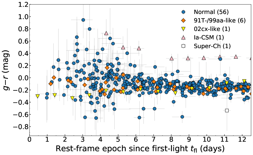
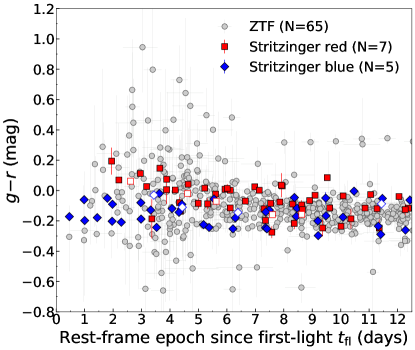
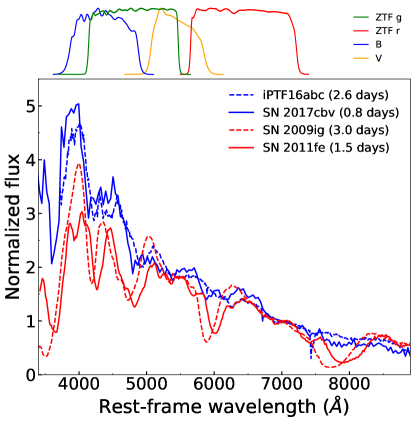
Figure 1 shows the $g-r$ colors for the sample of  SNe Ia discovered by ZTF within  days from first light $t_{\mathrm{fl}}$. The distribution of $g-r$ values is rather homogeneous starting from about  days after $t_{\mathrm{fl}}$, with colors clustering around $g-r\sim-0.15$ mag. In contrast, the scatter is found to be larger at earlier epochs. However, some fraction of the scatter observed at very early times is caused by the relatively high photometric uncertainties that characterize most of our SNe when first detected. In particular, the typical uncertainties at these early epochs have a median value of $\sigma_{\mathrm{noise}}\sim$  mag, while the $g-r$ distribution in the first  days after $t_{\mathrm{fl}}$ has a width of $\sigma$ =  mag. Following the light-curve rise and corresponding increase in signal-to-noise, both the uncertainties and the scatter in colors decrease, with the latter always $\sim 40\,\%$ larger than the former. Based on these numbers, we conclude that roughly half of the scatter observed in our colors at early times ($\lesssim$ 10 days) is intrinsic and half is due to photometric uncertainties, i.e., $\sigma_{\mathrm{int}}\sim\sigma_{\mathrm{noise}}\sim\sigma/\sqrt{2}$. The fact that $\sigma_{\mathrm{int}}\lesssim$  mag in the first days after first light suggests that SNe Ia are intrinsically more homogeneous in $g-r$ compared to what has been found in $B-V$ colors (Stritzinger et al., 2018). This is in qualitative agreement with the finding in Miller et al. (2020, see their section 4.3).

The larger homogeneity of $g-r$ relative to $B-V$ colors is confirmed when comparing our sample to the 12 SNe Ia from Stritzinger et al. (2018) that have available $g$ and $r$ photometry (Graham et al., 2015, 2017; Hsiao et al., 2015; Shappee et al., 2016; Hosseinzadeh et al., 2017; Burns et al., 2018; Miller et al., 2018; Vinkó et al., 2018) or early-time spectra to compute synthetic photometry (Foley et al., 2012; Silverman et al., 2012). As shown in Figure 2, no clear gap is found in $g-r$ at early phases between the “red” and “blue” class introduced in $B-V$ colors by Stritzinger et al. (2018), corroborating the idea that the early-time color evolution in SNe Ia might be rather homogeneous in $g$ and $r$ filters. Figure 2 also highlights how the color evolution of the ZTF sample is consistent with that reported by Stritzinger et al. (2018). The good agreement between the two samples gives us confidence about both the extinction- and $K$-corrections applied to our sample.

As shown in Figure 3, the larger homogeneity in $g-r$ compared to $B-V$ colors can be understood as a consequence of the different parts of the SED probed by different filter combinations. Early-time spectra of four SNe Ia in the Stritzinger et al. (2018) sample are shown, where two events (iPTF16abc and SN 2017cbv) are from the so-called “blue” class and two (SN 2009ig and SN 2011fe) are from the “red” class. In the wavelength region probed by the four filters, the largest spectral diversities between the two classes are seen at wavelengths below $\sim$ 4800 Å and around the Si ii $\lambda 6355$. These follow from “blue” objects being 91T-/99aa-like SNe, events that have been shown (e.g., Jeffery et al., 1992; Ruiz-Lapuente et al., 1992; Mazzali et al., 1995) to be more highly ionized than normal SNe Ia and thus lack singly-ionized absorption features such as Si ii $\lambda 6355$ at these early phases. The ZTF $g$ and $r$ filters are broader than $B$ and $V$ filters and cover both regions with large spectral diversity. In contrast, while the $B$ filter probes the region below $\sim$ 4800 Å, the $V$ filter covers a region around 5000 Å that is relatively homogeneous between the two classes. In addition, the $B$ filter extends to bluer wavelengths than the $g$ filter, in a spectral range ($\sim$ $3800-4200$ Å) with pronounced differences between “blue” and “red” objects. Therefore, the largest contrast between the two classes is captured by $B-V$ colors, while $g-r$ colors tend to wash out the observed spectral differences (this is similar to what is found at later epochs by Nordin et al. 2018, see top panel of their figure 3). This comparison explains why $g-r$ colors are found to be more homogeneous than $B-V$ in the first few days after explosion. At the same time, it suggests that $B$ and $V$ filters might be the better choice to test different models affecting the early-time colors.

3.2 Color evolution

Figure 4: Same as Figure 1 but with the $g-r$ evolution of each of the SNe highlighted. SNe are ordered from top-left to bottom-right according to their SALT2 $x_{1}$ values (Yao et al., 2019). Grey points mark the colors of the full sample for comparison. The red dashed line in each panel is a weighted least-square linear fit to colors in the first days for events with at least three data points in this time window. Colors and symbols are the same as in Figure 1.

Figure 4: Continued.

Figure 5: Comparison between observed and modelled slopes in the first  days since first light. The distribution refers to the linear slopes $\Delta(g-r)$/$\Delta t$ measured for SNe Ia with at least three detections in the first  days (see Section 3.2, the peculiar 02cx-like SN ZTF18abclfee/SN 2018cxk is not considered here). The range spanned by each series of models is shown with a shaded area and with an horizontal arrow. Mixing models are from Piro & Morozova (2016, red), Dessart et al. (2014, orange and violet) and Magee et al. (2020, purple), with an increasing amount of mixing from left to right (vertical lines). The range spanned by the four SN-companion interaction models from Kasen (2010) is shown in blue, while that from “double-detonation” models of Polin et al. (2019a) with $M_{\mathrm{He}}=0.01\,M_{\odot}$ in black. See text for more details.

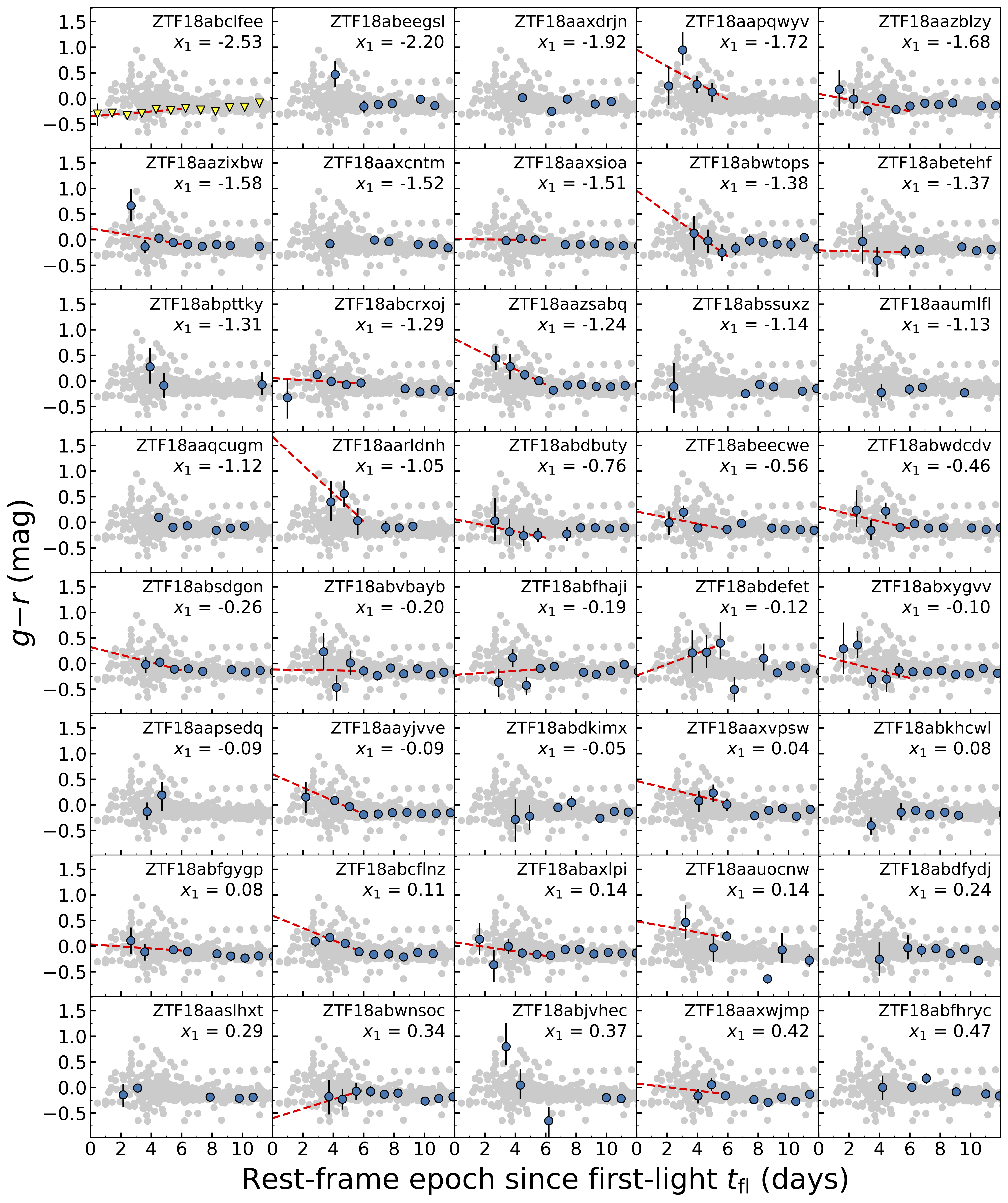
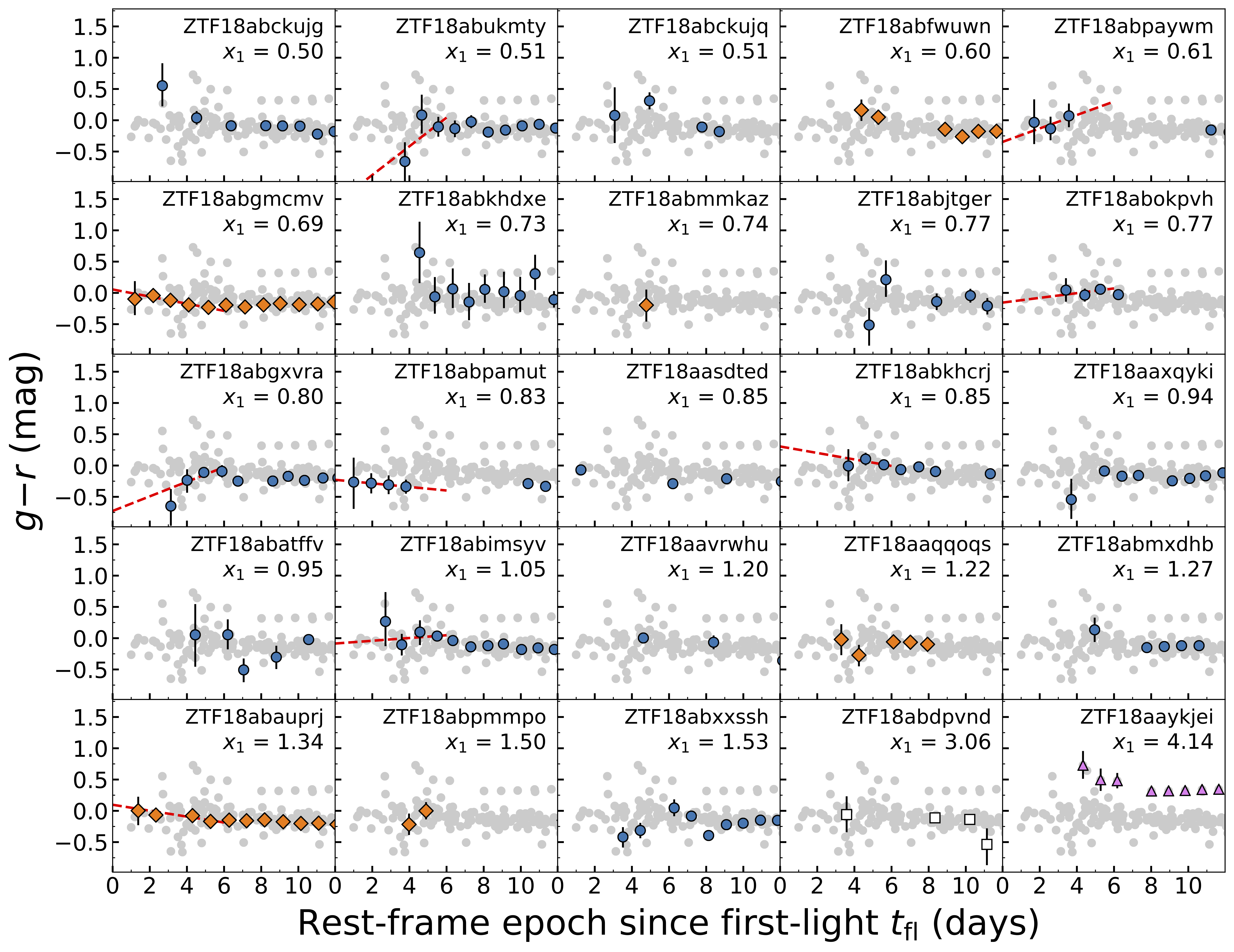
Despite the homogeneity of $g-r$ values discussed above, we do see a distinct color evolution. Figure 4 shows the $g-r$ color evolution of each individual SN in our sample. To characterize the change in colors we restrict ourselves to events that have at least three data-points in the first  days, resulting in a sample of  SNe Ia. We then characterize the color evolution by performing a weighted least-square linear fit to $g-r$ in the first  days and infer a slope $\Delta(g-r)$/$\Delta t$ for each SN, with positive (negative) values associated to colors becoming redder (bluer). Results of these fits are shown in Figure 4 and reported in Table 1 for the  SNe Ia that meet the criteria defined above.

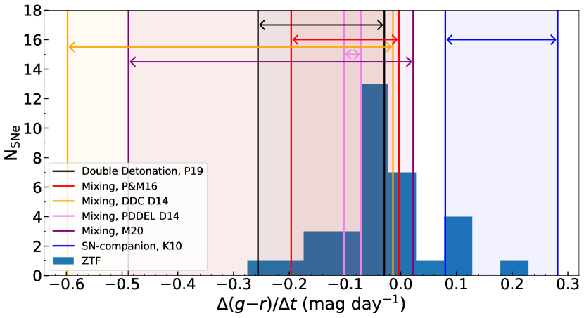
As shown in Figure 4, some events are characterized by a clear transition from redder to bluer colors and thus a negative slope, $\Delta(g-r)$/$\Delta t$ $<$ 0, others by a flatter evolution, $\Delta(g-r)$/$\Delta t$ $\sim$ 0. We note that all the three over-luminous 91T-/99aa-like SNe are characterized by relatively flat color evolutions, in agreement with findings from Stritzinger et al. (2018). The full range of slopes, going from a minimum of $\Delta(g-r)$/$\Delta t$ $\sim$ $-$0.28 to a maximum of $\Delta(g-r)$/$\Delta t$ $\sim$  mag day^-1, is reported in Figure 5. The range in color evolution is reminiscent of the two classes introduced by Stritzinger et al. (2018), with negative slopes consistent with their “red” class while flatter slopes with their “blue” class. When comparing data to models (Section 4) and when investigating the possible presence of multiple populations (Section 5), we will focus on the time evolution $\Delta(g-r)$/$\Delta t$  rather than the absolute values of colors. We consider this choice more robust as it is less sensitive to uncertainties introduced by both reddening corrections and $K$-corrections.

4 Comparison to models

In this section, we compare the $g-r$ evolution of our sample with model predictions. In particular, we focus on three different scenarios that have been shown to produce characteristic signatures in the colors at early times (see discussion in Section 1). Specifically, we explore the SN ejecta-companion interaction model (Section 4.1), the “double-detonation” scenario (Section 4.2) and models with different amounts of ⁵⁶Ni mixed throughout the ejecta (Section 4.3). The peculiar “02cx-like”, “Ia-CSM” and “Super-Chandrasekhar” events are not considered in these comparisons.

We note that models presented here are plotted relative to explosion, while data are shown relative to first light $t_{\mathrm{fl}}$. Many of the SNe Ia in our sample (especially those at low redshift) are detected 4 to 5 mag below peak (Yao et al., 2019) and thus $t_{\mathrm{fl}}-t_{\mathrm{exp}}$ is expected to be small for these events according to predictions from explosion models ($\lesssim 2$ days, see e.g., figure 4 in Dessart et al., 2014). Nevertheless, given the issues with inferring $t_{\mathrm{exp}}$ from observations and with having a common definition of $t_{\mathrm{fl}}$ across different models, we choose not to apply any shift to either models or data but caution against making a one-to-one comparison between them.

4.1 SN ejecta-companion interaction

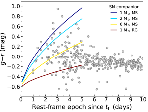
Figure 6 compares our sample to SN ejecta-companion models from Kasen (2010). Predicted colors are shown for the four different companion-star models discussed in Kasen (2010), i.e., three MS stars with different masses (1, 2 and 6 $M_{\odot}$) and a 1 $M_{\odot}$ RG star. Luminosity and temperature for each model is estimated using equation 22 and 25 in Kasen (2010) and assuming an ejecta velocity $v=10^{4}$ km s^-1 and an effective opacity $\kappa_{\mathrm{e}}=0.2$ cm² g^-1. Fluxes and corresponding $g-r$ colors are then estimated under a blackbody approximation. Curves are shown only in the first $\sim$ 5 days since first light when the emission from the SN ejecta-companion interaction is expected to be dominant (see e.g., equation 23 in Kasen, 2010; Maeda et al., 2018).

All the models investigated predict similar and relatively blue colors at first light, $g-r\sim-0.5$ mag, which then become redder with time following the decrease in temperature (see equation 25 in Kasen 2010). The transition from bluer to redder colors is characterized by $\Delta(g-r)$/$\Delta t$ $\gtrsim 0.1$ mag day^-1, with a slower evolution in the case the companion is a RG or for increasing masses in the MS case. As shown in Figure 5 and summarized in Table 1, we see evidence for such a rapid transition in events: ZTF18abgxvra (SN 2018efb), , , and ZTF18abpaywm (SN 2018fne). However, the latter characterized by relatively high photometric uncertainties (see Figure 5) while a sign of “red bump” in color evolution and might thus come from a “double-detonation” explosion (see Section 4.2 and right panel of Figure 7). Moreover, a good match in color slopes is found only with the 1 $M_{\odot}$ RG companion star model, which predicts a very strong bump in both UV and optical light curves (see figure 3 of Kasen, 2010) that is not found in any of these events.

Our calculations assume a perfect alignment between the exploding white dwarf, the companion star and the observer. As shown by Kasen (2010), the signature of the collision should be prominent $\sim$ 10$\%$ of the times for a favourable observer orientation near the perfect alignment. While we cannot exclude the presence of a companion star for each individual SN, the large size of our sample suggests we should see the effect of an interaction in $\sim$  events. As a consequence, the fact that we do not see any clear evidence for a SN ejecta-companion interaction poses challenges to this scenario to explain the bulk of the SN Ia population.

4.2 Helium-ignited Double Detonation models

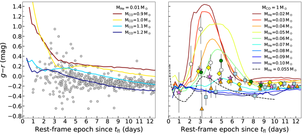
Figure 7 shows the $g-r$ evolution of our SNe Ia compared to that predicted by helium-ignited “double-detonation” models from the literature. The left panel includes models from Polin et al. (2019a) with fixed helium mass $M_{\mathrm{He}}=0.01\,M_{\odot}$ and varying carbon-oxygen core masses, while the right panel models from Noebauer et al. (2017) and Polin et al. (2019a) with carbon-oxygen core masses of $M_{\rm CO}\sim 1.0\,M_{\odot}$ and varying helium shell masses in the range $M_{\rm He}\in[0.02,0.10]\,M_{\odot}$.

Models with very thin helium layers (left panel) show a range in the early-time color slopes. Models with $M_{\rm CO}=0.9$ and $1.0\,M_{\odot}$ are characterized by steep transitions from red to bluer colors, while those with $M_{\rm CO}=1.1$ and $1.2\,M_{\odot}$ by flatter evolutions. As shown in Figure 5, this range in slopes is in reasonable agreement with that observed in our ZTF sample although it can not explain the events with $\Delta(g-r)$/$\Delta t$ $\gtrsim 0$ mag day^-1. We note that the four “double-detonation” models used here are those that have been claimed to explain maximum-light colors, velocity (Polin et al., 2019a), polarization (Cikota et al., 2019) and nebular calcium emission (Polin et al., 2019b) of a subset of SNe Ia. Our findings bring additional support to these claims, suggesting that the “double-detonation” scenario might contribute to some fraction of the observed SN Ia population. Specifically, the comparison in Figure 5 suggests that the “double detonation” models can explain the range in slopes observed for $\sim$ 60$\%$ ( out of ) of the events.

Models with relatively thicker helium layers ($0.02\lesssim M_{\rm He}\lesssim 0.07\,M_{\odot}$, right panel) produce strong “red bumps” (see Section 1). Visually inspecting the color evolution of each SN in Figure 4, we find evidence for a modest “red bump” in events: ZTF18abcflnz (SN 2018cuw), ZTF18abxxssh (SN 2018gvj), ZTF18abcrxoj (SN 2018cvw), ZTF18abgxvra (SN 2018efb), . All these events display $g-r$ colors that are relatively blue at detection, evolve to redder colors, reach $g-r\sim$ 0 at $\sim 3-$ days after $t_{\mathrm{fl}}$ and then turn over to bluer colors. This temporal evolution is in good agreement with predictions from e.g., Noebauer et al. (2017), suggesting that these SNe might come from “double-detonation” explosions of sub-$M_{\mathrm{ch}}$ white dwarfs with relatively thick helium layers ($M_{\mathrm{He}}\sim 0.05\,M_{\odot}$). In addition, ZTF18abxxssh (SN 2018gvj) is characterized by a strong light-curve excess at early times (Yao et al., 2019), making the interpretation of this SN within the “double-detonation” framework even more viable. The detection in out of SNe suggests a “red bump” might occur in $\sim$ $\%$ of the cases. We note that these estimates are not representative of the “double-detonation” contribution to the SN Ia population, but rather of a subclass with relatively thick helium mass and thus detectable “red bump”. As discussed above, “double-detonation” models with thin helium layers ($M_{\mathrm{He}}=0.01\,M_{\odot}$) might instead explain a good fraction ($\sim$ 60$\%$) of the observed population.

Figure 6: Comparison of our ZTF sample (grey points) to SN ejecta-companion models from Kasen (2010). Model predictions are shown for MS stars with three different masses (1, 2 and 6 $M_{\odot}$) and for a 1 $M_{\odot}$ RG star. Predicted colors are shown only in the first $\sim$ 5 days since $t_{\mathrm{fl}}$ when the emission from the SN ejecta-companion interaction is expected to be dominant (see e.g., equation 23 in Kasen, 2010).

Figure 7: Comparison of our ZTF sample to “double-detonation” models. Left panel: the full ZTF sample (grey points) compared to models from Polin et al. (2019a) with fixed helium mass $M_{\mathrm{He}}=0.01\,M_{\odot}$ and carbon-oxygen mass varying in the range $M_{\rm CO}\in[0.9,1.2]\,M_{\odot}$. Right panel: models with fixed carbon-oxygen mass $M_{\rm CO}=1.0\,M_{\odot}$ and varying helium masses. Models from Polin et al. (2019a, solid lines) have helium masses varying in the range $M_{\rm He}\in[0.02,0.10]\,M_{\odot}$ (from dark red to dark blue), while the model from Fink et al. (2010, black dashed line) as computed by Noebauer et al. (2017) has $M_{\rm He}=0.055\,M_{\odot}$. The events in the ZTF sample showing possible “red bumps”, ZTF18abcflnz (SN 2018cuw), ZTF18abxxssh (SN 2018gvj), ZTF18abcrxoj (SN 2018cvw), ZTF18abgxvra (SN 2018efb), are highlighted with yellow diamonds, light-blue squares, violet stars, orange triangles, respectively.

4.3 ⁵⁶Ni mixing

Figure 8: Comparison between our sample (grey points) and mixing models. The amount of mixing increases from models in red to models in blue. Top panel: models from Piro & Morozova (2016). Middle panel: delayed-detonation (DDC, solid and dashed lines) and pulsational delayed detonation (PDDEL, dotted lines) models from Dessart et al. (2014), together with the unpublished models DDC15m and PDDEL4m. Bottom panel: models from Magee et al. (2020) using the radiative transfer code turtls (Magee et al., 2018). For each mixing model, the shaded area represents color variations for different density profile shapes and kinetic energies (see text for details).

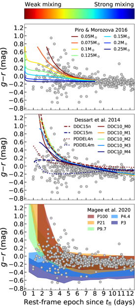
Figure 8 shows comparison between our sample and models exploring different amounts of ⁵⁶Ni mixing, where the color coding in all the different panels spans from red to blue for an increasing amount of mixing.

The top panel refers to models of Piro & Morozova (2016), where mixing is implemented using a “boxcar” average with widths between 0.05 and 0.25 $M_{\odot}$. As described in Section 1, models with stronger mixing are characterized by bluer colors at early times and relatively flatter evolution. Models by Piro & Morozova (2016) are qualitatively in good agreement with our data, both in terms of colors and color evolution (see Figure 5). This comparison tentatively suggests that some amount of mixing is required to reproduce the average colors in the first few days after first light. We note, however, that Local Thermodynamic Equilibrium (LTE) is assumed by Piro & Morozova (2016) and thus predicted colors should be treated with caution.

The middle panel of Figure 8 shows comparison with models by Dessart et al. (2014) and a more recent (and unpublished) incarnation (DDC15m, this model was computed using the same approach as in Dessart et al. 2014 and differs only in the strength of mixing, as explained below). Unlike in Piro & Morozova (2016), Dessart et al. (2014) carry out radiative transfer calculations for hydrodynamical models of $M_{\mathrm{ch}}$ delayed-detonations (denoted as DDC10 and DDC15). All elements are mixed using a boxcar algorithm adopting a characteristic velocity $v_{\mathrm{mix}}=$ 250 (DDC10$\_$M1), 500 (DDC10$\_$M2), 1000 (DDC10$\_$M3) and 1500 km s^-1 (DDC10$\_$M4). We also include the delayed-detonation model DDC15 (Dessart et al., 2014), characterized by a relatively weak mixing of elements (model DDC15n; $v_{\mathrm{mix}}=$ 400 km s^-1). In contrast, the new unpublished model DDC15m is strongly mixed and similar to the most mixed of the Piro & Morozova (2016) models (top panel of Figure 8). In model DDC15m, the mixing is done using $m_{\mathrm{mix}}=$ 0.25 $M_{\odot}$, together with a gaussian smoothing with a characteristic width of 300 km s^-1. These models also predict bluer and flatter colors for increasing amount of mixing, however, the colors in the first few days are relatively redder than those by Piro & Morozova (2016). This is caused in part by the fact that the mixing in mass space pollutes the outer (high velocity) ejecta layers much more efficiently that mixing in velocity space. This arises because little mass is contained in the high velocity layers of the ejecta (in model DDC10, there is about 0.2 $M_{\odot}$ beyond 15000 km s^-1). There may also be an opacity effect. Line blanketing below 5000 Å remains strong out to large velocities well above the optical photosphere, so that the SN optical color is only set at large velocity. Guessing the SN color at the photosphere by inspecting the local LTE temperature is inaccurate and likely overestimates the true optical color. The strongly mixed model DDC15m is about 0.15 mag redder than the most mixed model from Piro & Morozova, and appears somewhat too red relative to the observed mean $g-r$ color distribution (see also Dessart et al. 2014 and Miller et al. 2018). Although the colors are relatively redder than those observed, we note that the spread in slope predicted by the DDC10 and DDC15 suggests that some amount of mixing is required to explain the observed distribution shown in Figure 5.

Also included in the middle panel of Figure 8 are the pulsational delayed detonation models of Dessart et al. (2014). The explosion mechanism in this scenario is similar to the delayed-detonation mechanism but here a delay is introduced between the initial deflagration and the subsequent detonation (Hoeflich & Khokhlov, 1996). This first pulse partially unbinds the outer layers of the $M_{\mathrm{ch}}$ white dwarf, so that the delayed detonation leads to a strong interaction between the detonated inner ejecta and the marginally unbound outer ejecta. The interaction leads to a strong dissipation of kinetic energy into heat, the formation of a dense shell at around 10000 to 15000 km s^-1, with little mass beyond. Dessart et al. (2014) demonstrated that the early boost of the outer ejecta temperature had observable consequences for days on the luminosity and color, yielding brighter and bluer SNe. The models in Dessart et al. (2014) were however characterized by a weak mixing. Here, we recomputed the model PDDEL4 of Dessart et al. (2014) by using the same mixing recipe as for model DDC15m above. We refer to this model as PDDEL4m. For comparison, we include the weakly mixed model PDDEL4 (here called PDDEL4n) of Dessart et al. (2014). As can be seen from Figure 8, model PDDEL4m yields much bluer colors with a flatter evolution than the delayed detonation model DDC15m (i.e., with no pulsation). Because of the red-to-blue transition predicted in the first $\sim$ 3 days, this model struggles to reproduce the flatter-end of the observed $\Delta(g-r)$/$\Delta t$ distribution (see Figure 5).

The bottom panel of Figure 8 includes mixing models from Magee et al. (2020), computed using the radiative transfer code turtls (Magee et al., 2018). The grid of light-curve models is constructed with varying four main parameters: the ⁵⁶Ni mass (0.4, 0.6, 0.8 $M_{\odot}$), the density profile shape (double power law or exponential), the kinetic energy and the amount of ⁵⁶Ni mixing (see Magee et al. 2020 for more details). Here we compare our data to models producing 0.6 $M_{\odot}$ of ⁵⁶Ni and for each mixing value plot the range covered by different density profiles and kinetic energy. The comparison highlights how the observed $g-r$ evolution is well reproduced by models requiring some degree of ⁵⁶Ni mixing (see Figure 5). In particular, the strongest agreement with data in the first  days is found for the “P100”, “P21”, “P9.7” and “P4.4” mixing models, with $\sim$ % of the data-points falling in the color range predicted by these models. We note that the more stratified models “P100” and “P21” were disfavoured by Magee et al. (2020) based on comparisons to early light curves of normal SNe Ia.

Mixing is parametrized in all the models presented above and thus discrepancies with data do not necessarily rule out mixing scenarios but perhaps suggest that the mixing is different than adopted. Nevertheless, the range in slopes measured for our sample is in good agreement with the color evolution predicted by mixing models and better explained by incarnations requiring relatively strong ⁵⁶Ni mixing throughout the ejecta.

5 Testing for multiple populations

Figure 9: Top panel: test of multiple populations in the slope distribution, using a linear fit to the slope in the first days. The distribution is consistent with being drawn from a single population (i.e., one component), with multiple components strongly disfavoured ($\Delta$BIC $>6$, see text for details). Bottom panel: SALT2 $x_{1}$ parameter as a function of the linear slope $\Delta(g-r)$/$\Delta t$. A significant correlation is found (Pearson’s coefficient $\rho=$ , p-value=). The analysis is restricted to  SNe Ia with at least three detections in the first  days (the peculiar 02cx-like SN ZTF18abclfee/SN 2018cxk is excluded from this analysis). Symbols are the same as in Figure 1.

In this section, we take a closer look at the color evolution of $g-r$ colors at early phases, with the aim of testing the claim of two distinct populations made by Stritzinger et al. (2018, see Section 1). Specifically, we will base our discussion on  SNe Ia with reliable $g-r$ slopes in the first  days ($\Delta(g-r)$/$\Delta t$) as discussed in Section 3.2 (the peculiar 02cx-like SN ZTF18abclfee/SN 2018cxk is excluded from this analysis). In particular, we will first test the presence of multiple populations in Section 5.1 and then search for possible correlations between color evolution and brightness in Section 5.2.

5.1 Gaussian Mixture Models

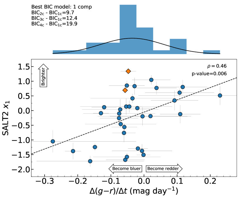
To test the claim of distinct populations, we apply Gaussian mixture models with single or multiple components to $\Delta(g-r)$/$\Delta t$. In order to select how many components best fit the data, we use the Bayesian information criteria (BIC, Schwarz 1978) defined as

$$\mathrm{BIC}=-2\,\mathrm{ln}\mathcal{L}+k\,\mathrm{ln}N~{}~{},$$ (2)

where $\mathcal{L}$ is the maximum likelihood, $N$ the number of data points and $k$ the number of parameters. The best model is the one with the lowest BIC, with the other models strongly disfavoured if the difference to the best-fit model, $\Delta$(BIC), is larger than 6 (see e.g., Sollerman et al., 2009). The difference between different IC approaches lies in how much multiple-component models (and thus an added complexity) are penalised compared to a single-component model. As discussed in Liddle (2004), we choose BIC as this penalizes complexity/number of parameters more compared to e.g., the Akaike information criteria (AIC, Akaike 1974).

Results of this analysis are summarized in the top panel of Figure 9, where we show the distribution of $\Delta(g-r)$/$\Delta t$ values together with the BIC best-fit model. We find BIC $\sim$  for models with one, two, three and four components, respectively. Therefore, the distribution is consistent with being drawn from one single population, i.e., min(BIC) = BIC_1C. In addition, a one-component is not only preferred but strongly favoured over multiple-component models ($\Delta$BIC $>6$).

To summarize, the color evolution in the first $\sim$  days after first light does not show any evidence for two or multiple components and it is consistent with being drawn from a single population. This conclusion is in contrast with the claim in Stritzinger et al. (2018) although we note that $B-V$ might be a better combination compared to $g-r$ to test for the presence of multiple populations (see Section 3.1). Our findings are consistent with the $B-V$ color evolution reported in Han et al. (2020, see their figure 5), where there appears to be no gap between the “red” and “blue” class when adding six events to the sample of Stritzinger et al. (2018). Surprisingly, Han et al. (2020) claims the presence of two distinct classes, although we note that similarly to Stritzinger et al. (2018) no analysis is provided to corroborate their conclusion.

5.2 Color evolution vs brightness

The bottom panel of Figure 9 show values of $\Delta(g-r)$/$\Delta t$ against the SALT2 $x_{1}$ parameter, where the latter is used as a proxy for the SN brightness (with brighter events corresponding to larger $x_{1}$). We find a moderate correlation between the linear slope $\Delta(g-r)$/$\Delta t$ and SALT2 $x_{1}$. Specifically, the Pearson’s correlation coefficient of $\rho=$  suggests that this correlation is significant (p-value of , i.e., statistically significant at the significance level of 0.01). Relatively brighter events (large $x_{1}$) are preferentially associated to $g-r$ colors that are flat or evolving to redder colors, $\Delta(g-r)$/$\Delta t$ $\gtrsim$ 0. In contrast, relatively fainter events (small $x_{1}$) are characterized by colors becoming bluer with time, $\Delta(g-r)$/$\Delta t$ $<$ 0.

To summarize, we find a moderate correlation between brightness and color slope in the first $\sim$  days, with brighter events preferentially associated to flatter evolutions while fainter SNe characterized by a transition from redder to bluer colors. These two behaviours are in qualitative agreement with those identified by Stritzinger et al. (2018) for their “blue” and “red” classes, respectively. However, our findings suggests that these are only the extremes of a continuous behaviour, thus arguing against a bimodality (Stritzinger et al., 2018, see also Section 5.1).

6 Discussion and conclusions

We presented $g-r$ colors for a sample of  SNe Ia discovered within  days from first light by ZTF in 2018. The size of our sample is the one available in the literature and extends to higher redshifts (up to $z=$ ). We find that $g-r$ colors are relatively homogeneous at all the phases investigated, from first light to $\sim$ two weeks after. In particular, the observed scatter of $\sim$ 1.5 mag at very early phases ($\lesssim$  days) is roughly half intrinsic and half due to high photometric uncertainties. Specifically, we find that the intrinsic dispersion in $g-r$ colors in the first few days after explosion is smaller than that found in $B-V$ colors (Stritzinger et al., 2018) as a consequence of the different wavelength regions probed by different filter combination (Nordin et al., 2018).

We do, however, note different behaviours in the color evolution from first light to $\sim$  days later. In particular, some events have a rather steep change from redder to bluer colors while others are characterized by a flatter evolution. We further identify a significant correlation ($\rho=$ , p-value of ) between the SALT2 $x_{1}$ parameter and the linear color slope in the first  days, indicating that brighter events (large $x_{1}$) have flatter color evolutions at early times. However, contrary to previous claims in the literature (Stritzinger et al., 2018), the slope distribution does not show any evidence for bimodality and it is consistent with being drawn from a single population. We note that our findings are based on a sub-sample of normal SNe Ia with at least three detections in the first days since first light, a sample that is about the one in the literature after applying the same criteria (Stritzinger et al., 2018; Han et al., 2020).

The range in early-time slopes is reminiscent of mixing models, where an increasing amount of ⁵⁶Ni mixing in the outer ejecta regions leads to a transition from colors rapidly changing from red to blue to colors with a flatter evolution. In this context, the correlation found between early-time color slopes and brightness suggests that stronger mixing (hence flatter color evolution) might occur in explosions producing more ⁵⁶Ni (hence brigther). At the same time, the range in early-time slopes is in good agreement with predictions from helium-ignited “double-detonation” models with very thin helium layers ($M_{\mathrm{He}}=0.01\,M_{\odot}$) and varying carbon-oxygen masses between $0.9$ and $1.2\,M_{\odot}$ (Polin et al., 2019a). In addition,  SNe in our sample show evidence for a distinctive early-time “red bump” predicted by “double-detonation” models with larger helium masses ($0.02\,M_{\odot}\lesssim M_{\mathrm{He}}\lesssim 0.07\,M_{\odot}$, Noebauer et al., 2017; Polin et al., 2019a). Our findings support recent claims in the literature arguing that a subset of SNe Ia originates from “double-detonation” explosions (Cikota et al., 2019; Polin et al., 2019a, b). In contrast, we find no clear evidence for a rapid transition from blue to red colors predicted by the ejecta-companion model discussed by Kasen (2010), posing serious challenges to this scenario for explaining the bulk of SNe Ia.

Based on the number of young SNe Ia discovered from May to December 2018 and presented here, the 3-year ZTF survey is expected to have a final sample of at least $\sim$  SNe Ia discovered within days from first light. Such a large sample will allow us to place stronger constraints on explosion models and test the possible correlation between color evolution and brightness identified in this work.

References

- Akaike (1974) Akaike, H. 1974, IEEE Transactions on Automatic Control, 19, 716
- Bellm et al. (2019) Bellm, E. C., Kulkarni, S. R., Graham, M. J., et al. 2019, PASP, 131, 018002
- Branch et al. (2006) Branch, D., Dang, L. C., Hall, N., et al. 2006, PASP, 118, 560
- Burns et al. (2014) Burns, C. R., Stritzinger, M., Phillips, M. M., et al. 2014, ApJ, 789, 32
- Burns et al. (2018) Burns, C. R., Parent, E., Phillips, M. M., et al. 2018, ApJ, 869, 56
- Cikota et al. (2019) Cikota, A., Patat, F., Wang, L., et al. 2019, MNRAS, 490, 578
- De et al. (2019) De, K., Kasliwal, M. M., Polin, A., et al. 2019, ApJ, 873, L18
- Dessart et al. (2014) Dessart, L., Blondin, S., Hillier, D. J., & Khokhlov, A. 2014, MNRAS, 441, 532
- Dimitriadis et al. (2019) Dimitriadis, G., Foley, R. J., Rest, A., et al. 2019, ApJ, 870, L1
- Fink et al. (2010) Fink, M., Röpke, F. K., Hillebrandt, W., et al. 2010, A&A, 514, A53
- Foley et al. (2012) Foley, R. J., Challis, P. J., Filippenko, A. V., et al. 2012, ApJ, 744, 38
- Graham et al. (2019) Graham, M. J., Kulkarni, S. R., Bellm, E. C., et al. 2019, PASP, 131, 078001
- Graham et al. (2015) Graham, M. L., Foley, R. J., Zheng, W., et al. 2015, MNRAS, 446, 2073
- Graham et al. (2017) Graham, M. L., Kumar, S., Hosseinzadeh, G., et al. 2017, MNRAS, 472, 3437
- Han et al. (2020) Han, X., Zheng, W., Stahl, B. E., et al. 2020, ApJ, 892, 142
- Hoeflich & Khokhlov (1996) Hoeflich, P., & Khokhlov, A. 1996, ApJ, 457, 500
- Hosseinzadeh et al. (2017) Hosseinzadeh, G., Sand, D. J., Valenti, S., et al. 2017, ApJ, 845, L11
- Hsiao et al. (2007) Hsiao, E. Y., Conley, A., Howell, D. A., et al. 2007, ApJ, 663, 1187
- Hsiao et al. (2015) Hsiao, E. Y., Burns, C. R., Contreras, C., et al. 2015, A&A, 578, A9
- Iben & Tutukov (1984) Iben, I., J., & Tutukov, A. V. 1984, ApJS, 54, 335
- Jacobson-Galan et al. (2019) Jacobson-Galan, W. V., Polin, A., Foley, R. J., et al. 2019, arXiv, arXiv:1910.05436
- Jeffery et al. (1992) Jeffery, D. J., Leibundgut, B., Kirshner, R. P., et al. 1992, ApJ, 397, 304
- Jiang et al. (2018) Jiang, J.-a., Doi, M., Maeda, K., & Shigeyama, T. 2018, ApJ, 865, 149
- Jiang et al. (2017) Jiang, J.-A., Doi, M., Maeda, K., et al. 2017, Nature, 550, 80
- Kasen (2010) Kasen, D. 2010, ApJ, 708, 1025
- Kasliwal et al. (2019) Kasliwal, M. M., Cannella, C., Bagdasaryan, A., et al. 2019, PASP, 131, 038003
- Li et al. (2019) Li, W., Wang, X., Vinkó, J., et al. 2019, ApJ, 870, 12
- Liddle (2004) Liddle, A. R. 2004, MNRAS, 351, L49
- Livio & Mazzali (2018) Livio, M., & Mazzali, P. 2018, Phys. Rep., 736, 1
- Livne (1990) Livne, E. 1990, ApJ, 354, L53
- Maeda et al. (2018) Maeda, K., Jiang, J.-a., Shigeyama, T., & Doi, M. 2018, ApJ, 861, 78
- Magee et al. (2020) Magee, M. R., Maguire, K., Kotak, R., et al. 2020, A&A, 634, A37
- Magee et al. (2018) Magee, M. R., Sim, S. A., Kotak, R., & Kerzendorf, W. E. 2018, Astronomy and Astrophysics, 614, A115
- Masci et al. (2019) Masci, F. J., Laher, R. R., Rusholme, B., et al. 2019, PASP, 131, 018003
- Mazzali et al. (1995) Mazzali, P. A., Danziger, I. J., & Turatto, M. 1995, A&A, 297, 509
- Miller et al. (2018) Miller, A. A., Cao, Y., Piro, A. L., et al. 2018, ApJ, 852, 100
- Miller et al. (2020) Miller, A. A., Yao, Y., Bulla, M., et al. 2020, arXiv, arXiv:2001.00598
- Moll & Woosley (2013) Moll, R., & Woosley, S. E. 2013, ApJ, 774, 137
- Noebauer et al. (2017) Noebauer, U. M., Kromer, M., Taubenberger, S., et al. 2017, MNRAS, 472, 2787
- Nomoto (1980) Nomoto, K. 1980, Space Sci. Rev., 27, 563
- Nordin et al. (2018) Nordin, J., Aldering, G., Antilogus, P., et al. 2018, A&A, 614, A71
- Nugent et al. (2011) Nugent, P. E., Sullivan, M., Cenko, S. B., et al. 2011, Nature, 480, 344
- Papadogiannakis et al. (2019) Papadogiannakis, S., Goobar, A., Amanullah, R., et al. 2019, MNRAS, 483, 5045
- Piro & Morozova (2016) Piro, A. L., & Morozova, V. S. 2016, ApJ, 826, 96
- Polin et al. (2019a) Polin, A., Nugent, P., & Kasen, D. 2019a, ApJ, 873, 84
- Polin et al. (2019b) —. 2019b, arXiv, arXiv:1910.12434
- Riess et al. (1999) Riess, A. G., Filippenko, A. V., Li, W., et al. 1999, AJ, 118, 2675
- Ruiz-Lapuente et al. (1992) Ruiz-Lapuente, P., Cappellaro, E., Turatto, M., et al. 1992, ApJ, 387, L33
- Schwarz (1978) Schwarz, U. J. 1978, A&A, 65, 345
- Shappee et al. (2016) Shappee, B. J., Piro, A. L., Holoien, T. W.-S., et al. 2016, ApJ, 826, 144
- Shappee et al. (2019) Shappee, B. J., Holoien, T. W. S., Drout, M. R., et al. 2019, ApJ, 870, 13
- Silverman et al. (2012) Silverman, J. M., Ganeshalingam, M., Cenko, S. B., et al. 2012, ApJ, 756, L7
- Sollerman et al. (2009) Sollerman, J., Mörtsell, E., Davis, T. M., et al. 2009, ApJ, 703, 1374
- Spiegelhalter et al. (2002) Spiegelhalter, D. J., Best, N. G., Carlin, B. P., & Van Der Linde, A. 2002, Journal of the royal statistical society: Series b (statistical methodology), 64, 583
- Stritzinger et al. (2018) Stritzinger, M. D., Shappee, B. J., Piro, A. L., et al. 2018, ApJ, 864, L35
- Taam (1980) Taam, R. E. 1980, ApJ, 237, 142
- Vallely et al. (2019) Vallely, P. J., Fausnaugh, M., Jha, S. W., et al. 2019, MNRAS, 487, 2372
- Vinkó et al. (2018) Vinkó, J., Ordasi, A., Szalai, T., et al. 2018, PASP, 130, 064101
- Webbink (1984) Webbink, R. F. 1984, ApJ, 277, 355
- Whelan & Iben (1973) Whelan, J., & Iben, Icko, J. 1973, ApJ, 186, 1007
- Yao et al. (2019) Yao, Y., Miller, A. A., Kulkarni, S. R., et al. 2019, ApJ, 886, 152