Calculation of $\pi$ on the IBM quantum computer and the accuracy of one-qubit operations

A quantum algorithm for the calculation of $\pi$ is proposed and implemented on the five-qubit IBM quantum computer with superconducting qubits. We find $\pi=3.157\pm 0.017$. The error is due to the noise of quantum one-qubit operations and measurements. The results can be used for estimating the errors of the quantum computer and suggest that the errors are purely random.

1 Introduction

Many problems were considered for the IBM quantum computer with superconducting qubits [1, 2], but high levels of noise preclude solving most of them. The problem of decreasing the noise and increasing the computation accuracy remains very important. Various schemes for solving the noise problem were considered [3, 4, 5]. There were also some proposals for the tasks suitable for existing quantum computers [6, 7, 8, 9].

In this paper, we do not try to best classical computers with a quantum one. Instead, we focus on a classical problem that has long been used to highlight the capabilities of classical computers and the power of applied mathematics in the era before computers. The problem consists in computing the number $\pi$.

Arguably, Archimedes’ results for $\pi$ from 23 centuries ago have been sufficiently accurate for many applications. Nevertheless, a truly gigantic number of digits has been computed since then. We do not attempt to beat the existing records and focus on getting the best result for $\pi$ we can extract with the IBM quantum computer.

Our algorithm uses only one-qubit operations. We apply our results to estimate the accuracy of the quantum computer. The precise error rate of an early computer might not be of great interest, but the nature of its errors is. Are the dominant errors random or systematic? Our findings are consistent with purely random errors.

This article is organized as follows. In Sec. 2, the idea of the computational method is presented. The algorithm for calculatiing $\pi$ on a quantum computer is given in Sec. 3. We briefly summarize our results in the concluding Sec. 4.

2 The idea

Let us consider a qubit in the initial state $\left|0\right>$. After “rotating” it by $\varphi$ radians (on the Bloch sphere) around the $y$-axis, its state will be $\exp(-iI_{y}\varphi)\left|0\right>$. ($\varphi$ is thus the dimensionless time). If it is subsequently measured in the basis $\{\left|0\right>,\,\left|1\right>\}$, then the outcome will be $\left|0\right>$ with the probability $\cos^{2}(\varphi/2)=(1+\cos\varphi)/2$ and $\left|1\right>$ with the probability

$$p(\varphi)=\sin^{2}(\varphi/2)=(1-\cos\varphi)/2.$$ (1)

The difference between any two successive roots of the equation $p(\varphi)=1/2$, for example, $\pi/2$ and $3\pi/2$, is exactly $\pi$. Hence, $\pi$ can be determined from the knowledge of $p(\varphi)$. Of course, we cannot measure $p(\varphi)$ exactly. On a real quantum device, we cannot even guarantee that the rotation angle is exactly as desired. We expect, however, that the real rotation angle $\varphi=ct$, where $t$ is a value which can be precisely controlled (such as the duration of a control pulse) and $c$ is a constant. Thus, we can estimate $p(ct)$ for a given $t=\varphi/c$ as the fraction $f(t)$ of the measurements that give the result $\left|1\right>$. To proceed further with calculating $\pi$, we need to estimate the value of $c$ as well.

Estimation of the constant $c$

Below, we will use the notation $t_{1}=\pi/2c$ and $t_{2}=3\pi/2c$. These are the first two nonnegative roots of the equation $p(ct)=1/2$. Since

$$\int\limits_{t_{1}}^{t_{2}}\left(p(ct)-\frac{1}{2}\right)\,dt=\frac{1}{c},$$ (2)

(see Eq. (1)), the area under the experimental curve $\left(f(t)-\frac{1}{2}\right)$ on the interval $[\hat{t}_{1},\hat{t}_{2}]$ (where the hats denote an estimate of the respecitve variable) provides a way to estimate $c$.

Due to the experimental imperfections, $\left|0\right>$ and $\left|1\right>$ cannot be obtained with certainty, no matter what operations are performed. For the sake of estimating errors, we approximate the experimental probability of obtaining the result $\left|1\right>$ as

$$P(t)=\alpha\frac{1-\cos(ct+\phi_{0})}{2}+\beta,$$ (3)

with three empirical constants $\alpha$, $\beta$, $\phi_{0}$ in addition to $c$. That is, $P(t)$ is derived from $p(\varphi)$ by arbitrary linear transforms of both its domain (with parameters $c$ and $\phi_{0}$) and the image (with parameters $\alpha$ ,$\beta$). These empirical parameters allow us to account for the initial state not being exactly $\left|0\right>$ (it could even be mixed) and measurement errors. In the ideal case $\alpha=1$, $\beta=\phi_{0}=0$. In any case $\alpha\geq 0$, $0<\beta<1-\alpha$, since the probability must be between 0 and 1.

3 The algorithm

We assume that the approximate period of $P(t)$ is already known, and time units are chosen so that it is approximately 6. The fraction $f(t)$ will often be called simply “fraction”. Let $T$ be the set of all values of $t$ for which the experiments were performed.The algorithm consists of the following steps:

1. Roughly estimate $\alpha$ and $\beta$ (the measurement imperfections): find $\hat{\alpha}$, $\hat{\beta}$ from the system of equations

   $$\left\{\begin{aligned} \min\limits_{t}f(t)&=\hat{\beta}\\ \max\limits_{t}f(t)&=\hat{\alpha}+\hat{\beta}\end{aligned}\right.$$ (4)

2. Normalize $f(t)$ so that its minimum is 0 and maximum is 1:

   $$f_{1}(t)=\frac{f(t)-\hat{\beta}}{\hat{\alpha}}$$

3. Define $\tilde{f}_{1}(t)$ as the extension of $f_{1}$ for values of $t$ between $\min T$ and $\max T$ by linear interpolation between neighboring values of $f_{1}(t)$.

4. Roughly estimate $t_{1}$ and $t_{2}$: find two time instants $t$ such that $\tilde{f}(t)=0.5$ using root search methods, $\hat{t}_{1}$ starting from the point $t=1.5$ and $\hat{t}_{2}$ starting from $t=4.5$.

5. Refine the estimate for $\alpha$ and $\beta$: solve the system

   $$\left\{\begin{aligned} \mathrm{mean}&\left\{f_{1}(t)\middle|\,|t-\hat{t}_{minval}|<\delta\right\}=&\hat{\beta}&\\ \mathrm{mean}&\left\{f_{1}(t)\middle|\,|t-\hat{t}_{maxval}|<\delta\right\}=&\hat{\alpha}+\hat{\beta}&\end{aligned}\right.$$ (5)

   where $\mathrm{mean}\,S$ is the arithmetic mean of the set $S$, $\hat{t}_{maxval}=\frac{\hat{t}_{1}+\hat{t}_{2}}{2}$ is the estimated maximum point of $P(t)$ calculated from $t_{1}$ and $t_{2}$, similarly for $\hat{t}_{minval}$; $\delta$ is chosen so that $1-\cos(c\delta)\ll{\sqrt{P(t)(1-P(t))}}$. (The right-hand side is the standard deviation of a Bernoulli distribution.)

6. Repeat step 2 with new $\hat{\alpha}$ and $\hat{\beta}$.

7. Refine the estimate for $t_{1}$ and $t_{2}$ as follows. For $i=1,2$:

   1. take the experimental times $t$ such that $|t-t_{i}|\leq 0.5$ and corresponding $f_{1}(t)$

   2. fit a linear function $\gamma t+k$ to these $f_{1}(t)$ by the least-squares method

   3. the new $\hat{t}_{i}$ is a solution to the equation $\gamma\hat{t}_{i}+k=0.5$

8. Find the integral $I=\int\limits_{t_{1}}^{t_{2}}\left(f(t)-\frac{1}{2}\right)\,dt$ using the trapezoidal rule.

9. Estimate $\pi$ as $\frac{t_{2}-t_{1}}{I}$.

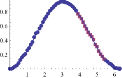
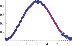
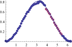
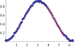
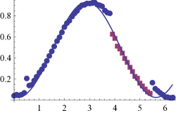
We made 8192 measurements on each of the five qubits for each time instant from 0 to 6.3 with the step of 0.1. The value $\delta=0.1$ (see step 5) was chosen. Each value of $t$ required a separate job on the quantum platform. The results on qubit #5 (Fig. 1(e)) contain a large jump near $t=4$, apparently due to a calibration difference between our runs. In the graph for qubit #3 (Fig. 1(c)), a step near the time instant $t=\pi$ can also be observed. The results from those qubits were discarded. The results on the three remaining qubits are well described by Eq. (3) in the region of interest ($1<t<5$). The dependence of the fractions on $t$ is plotted in Fig. 1. On the three plots corresponding to those qubits, the points are, for the most part, close to the theoretical curve.

Checking the algorithm’s accuracy

In order to check the accuracy of the algorithm, we estimated parameters $\alpha$ and $\beta$ for the three qubits used in the experiment from experimental data; generated synthetic data with the probabilities according to Eq. (3) for time instants $t$ as in the experiment (see above); ran the algorithm 50 times for each of three (estimated) pairs $(\alpha,\beta)$, for a total of 150 times; and calculated the standard deviation of the result.

This also allows to measure the impact of random errors on any intermediate result produced by the algorithm, in the same way. We found that the standrard deviation of $(t_{2}-t_{1})$ is 0.009 and the standard deviation of $I$ is 0.006.

The comments on the accuracy of the algorithm below and our conclusion that random errors exceed systematic ones are based on this calculation.

After performing the calculation with the above algorithm and averaging the results from different qubits, we obtain the result $\pi\approx 3.157\pm 0.017$ (2 standard deviations calculated as described above).

(a) Qubit #1

(b) Qubit #2

(c) Qubit #3

(d) Qubit #4

(e) Qubit #5

Figure 1: Experimental fractions of $\left|1\right>$ measurement outcomes (points) and curves obtained by fitting parameters in Eq. (3) (solid line). Qubits #1 (a), #2 (b), #3 (c), #4 (d) and #5 (e). Horizontal axis is the rotation angle $t$

Discussion

Using more complicated integration rules such as Simpson’s rule is pointless in our case, as it won’t be more accurate. In the case $c=1$, calculating the theoretical value of integral $I$ by the trapezoidal rule with time step of 0.1 gives the value of 0.99917 instead of the exact value $I=1$. Thus, the error due to the trapezoidal rule is small compared to the error due to limited number of measurements in our case (standard deviation is about 0.006, with the magnitude of measurement errors we observed; it would be 0.0023 in the ideal case) or the estimation error of $(t_{2}-t_{1})$.

A possible way to improve the accuracy of the results would be to measure several periods of $p(t)$ instead of half a period, assuming that decoherence is small enough.

4 Conclusions

We suggested a simple quantum algorithm for calculating $\pi$ on a quantum computer and implemented it on the IBM quantum platform. We provide an estimate of the magnitude of random errors and show that our results are consistent with the hypothesis of errors being purely random. The computed value of $\pi=3.157$ is within its error bars $\pm 0.017$ from the correct value. This accuracy is still behind the celebrated result $3\frac{10}{71}<\pi<3\frac{1}{7}$ by Archimedes, but it seems that the achievements of classical antiquity are within reach of modern quantum information science.

Acknowledgements

This work was performed as a part of a state task (State Registration No. 0089-2019-0002). This work is partially supported by the Russian Foundation for Basic Research (grants № 19-32-80004 and № 20-03-00147). The authors are grateful to D. E. Feldman for useful discussion.

References

- [1] Jens Koch, Terri M. Yu, Jay Gambetta, A. A. Houck, D. I. Schuster, J. Majer, Alexandre Blais, M. H. Devoret, S. M. Girvin, and R. J. Schoelkopf. Charge-insensitive qubit design derived from the Cooper pair box. Phys. Rev. A, 76:042319, Oct 2007.
- [2] Jerry M. Chow, Jay M. Gambetta, Easwar Magesan, David W. Abraham, Andrew W. Cross, B. R. Johnson, Nicholas A. Masluk, Colm A. Ryan, John A. Smolin, Srikanth J. Srinivasan, and M. Steffen. Implementing a strand of a scalable fault-tolerant quantum computing fabric. Nature Communications, 5:4015, 2014.
- [3] Kristan Temme, Sergey Bravyi, and Jay M. Gambetta. Error mitigation for short-depth quantum circuits. Phys. Rev. Lett., 119:180509, Nov 2017.
- [4] Abhinav Kandala, Kristan Temme, Antonio D. Córcoles, Antonio Mezzacapo, Jerry M. Chow, and Jay M. Gambetta. Error mitigation extends the computational reach of a noisy quantum processor. Nature, 567:491–495, 2019.
- [5] A.D. Córcoles, Easwar Magesan, Srikanth J. Srinivasan, Andrew W. Cross, M. Steffen, Jay M. Gambetta, and Jerry M. Chow. Demonstration of a quantum error detection code using a square lattice of four superconducting qubits. Nature Communications, 6:6979, 2015.
- [6] A.A. Zhukov, S.V. Remizov, W.V. Pogosov, and E.Yu. Lozovik. Algorithmic simulation of far-from-equilibrium dynamics using quantum computer. Quantum Information Processing, 17:223, 2018.
- [7] S. I. Doronin, E. B. Fel’dman, and A. I. Zenchuk. Solving systems of linear algebraic equations via unitary transformations on quantum processor of IBM Quantum Experience. Quantum Information Processing, 19(2):68, 2020.
- [8] Abhinav Kandala, Antonio Mezzacapo, Kristan Temme, Maika Takita, Markus Brink, Jerry M. Chow, and Jay M. Gambetta. Hardware-efficient variational quantum eigensolver for small molecules and quantum magnets. Nature, 549:242–246, 2017.
- [9] Ying Li and Simon C. Benjamin. Efficient variational quantum simulator incorporating active error minimization. Phys. Rev. X, 7:021050, Jun 2017.