Upper edge of chaos and the energetics of transition in pipe flow
Abstract
In the past two decades, our understanding of the transition to turbulence in shear flows with linearly stable laminar solutions has greatly improved. Regarding the susceptibility of the laminar flow, two concepts have been particularly useful: the edge states and the minimal seeds. In this nonlinear picture of the transition, the basin boundary of turbulence is set by the edge state’s stable manifold and this manifold comes closest in energy to the laminar equilibrium at the minimal seed. We begin this paper by presenting numerical experiments in which three-dimensional perturbations are too energetic to trigger turbulence in pipe flow but they do lead to turbulence when their amplitude is reduced. We show that this seemingly counter-intuitive observation is in fact consistent with the fully nonlinear description of the transition mediated by the edge state. In order to understand the physical mechanisms behind this process, we measure the turbulent kinetic energy production and dissipation rates as a function of the radial coordinate. Our main observation is that the transition to turbulence relies on the energy amplification away from the wall, as opposed to the turbulence itself, whose energy is predominantly produced near the wall. This observation is further supported by the similar analyses on the minimal seeds and the edge states. Furthermore, we show that the time-evolution of production-over-dissipation curves provide a clear distinction between the different initial amplification stages of the transition to turbulence from the minimal seed.
I Introduction
Transition to turbulence in shear flows with linearly stable laminar solutions has baffled researchers since the seminal experiments of Reynolds Reynolds (1883) for more than a century. Despite its ubiquity in the nature and applications, many aspects of this phenomenon have only recently been understood, in part thanks to the availability of new computational and experimental tools. In our new understanding of the transition without a linear instability, turbulence is triggered by finite-amplitude disturbances to the laminar flow that push the state across the so-called “edge of chaos” (Skufca et al., 2006), which separates perturbations that can trigger turbulence from those that cannot. This description of transition follows a fully nonlinear geometrical approach to the problem, which adopts ideas from the dynamical systems theory.
Fluid motion through a channel or a pipe can be thought of as a trajectory in the infinite-dimensional state space of the attainable velocity fields. This viewpoint of the fluid dynamics was put forward by Hopf Hopf (1948), who also conjectured that the turbulence should asymptotically be confined in a finite-dimensional manifold in the state space due to the presence of dissipation in the governing Navier-Stokes equations. While a rigorous proof of whether this indeed is the case is yet to be found, the assumption of finite-dimensionality is tacit in all computational fluid dynamics, where the velocity fields are expressed on a finite grid or an equivalent spectral expansion. In fact, a finite-dimensional numerical representation constitutes an approximation to the infinite dimensional state space. If each numerical degree-of-freedom is assigned to an axis, then a snapshot of the fluid is a point in this high-dimensional space and its time-evolution under the Navier-Stokes equation is a trajectory.
Once the dynamical systems viewpoint is established, the transition question becomes a geometrical one. Which initial points in the state space eventually connects to the turbulence? Or conversely, which initial conditions decay onto the laminar equilibrium as they are evolved in time? In low dimensional chaotic systems with coexisting attracting sets, the basin boundary between the attractors is often found to be the stable manifold of a saddle-type invariant solution (Alligood et al., 1997; Grebogi et al., 1982, 1983). In numerical studies of such systems, the saddle-type solutions can be probed via a bisection algorithm that refines initial conditions between those that end up in either attractor, yielding an approximation of an initial condition on the stable manifold of the saddle solution. In the case of transition to turbulence without a linear instability of the laminar solution, any initial condition that is weak enough will decay. Thus, if an initial condition that yields turbulence is found, then this initial condition could be scaled down until it can no longer trigger the transition, in order to initiate a bisection algorithm. Through such a bisection search in a computational study of channel flow, Itano & Toh Itano and Toh (2001) found the basin boundary between laminar and turbulence in channel flow to be set by a traveling wave solution of the saddle-type. On a reduced-order model of a shear flow, Skufca et al. Skufca et al. (2006) showed that the asymptotic dynamics on the laminar-turbulent boundary can be periodic, or even chaotic. Similar computational studies of shear flows (Toh and Itano, 2003; Schneider et al., 2007, 2008; Mellibovsky et al., 2009; Schneider et al., 2010; Zammert and Eckhardt, 2014; Khapko et al., 2016) yielded various types of asymptotic states in the laminar-turbulent boundary. In most of the current literature, irrespective of the type of their time-dependence, such asymptotic states at the laminar-turbulent boundary are referred to as the “edge states”; and the bisection-based methods that probe edge states are called “edge tracking”. In the pipe flow setting, which we are going to consider in the current study, the edge state appears to be chaotic with transient visits to traveling wave solutions (Budanur and Hof, 2018).
If, in the subcritical regime, only some initial disturbances of sufficiently large energy can trigger transition, then a key question, both from a practical and scientific viewpoint, is the following. What is the weakest perturbation that is strong enough to trigger turbulence? The practical importance of identifying such minimal perturbations is due to the fact that avoiding them would be crucial in settings where turbulence is undesirable. In the edge state picture, such a minimal perturbation is the one that touches the stable manifold of the edge state at the point where the distance –in some norm– between the manifold and the laminar solution is the shortest. Pringle et al. Pringle and Kerswell (2010) formulated a nonlinear optimization method for identifying “minimal seeds” for triggering turbulence by searching for perturbations to the laminar flow whose energies amplified the most in a finite time horizon. Pringle et al. Pringle and Kerswell (2010) and other studies (Pringle et al., 2012; Duguet et al., 2013; Cherubini and Palma, 2014; Kerswell et al., 2014) demonstrated that the time-forward dynamics of minimal seeds indeed approach the edge states, evidencing that the minimal seeds lie on the edge states’ stable manifold. The flow structures of the minimal perturbations appeared completely different from those that can be expected from weakly nonlinear theories, demonstrating the strongly nonlinear nature of the transition problem. The energy growth of the minimal seed was found to occur via three mechanisms, coupled together by the nonlinear effects to produce a larger overall growth than a linear optimal. The initially fully localized streaks are slightly unwrapped and tilted away from the wall by the inviscid Orr process. This is then followed by the oblique-wave mechanism in which the helical modes quickly grow transiently and feed energy into the streamwise-independent modes. In the last phase, the well-known lift-up process, the streamwise rolls experience non-normal energy growth and advect the shear to drive the streaks. The Orr and oblique-wave phases occur in a very short time scale (less than 4 advective units) and give rise to most of the growth experienced by the minimal seed. By comparing the energy of the minimal seed at different phases of its evolution with the critical energies of different randomized disturbances, Marensi et al. Marensi et al. (2019) showed that the minimal seed, despite being quite ‘special’, evolves to a structure more similar to a ‘natural’ disturbance during the Orr and oblique-wave phases. In particular, the minimal seed at the end of the oblique-wave phase was found to be a reasonable proxy to characterize the critical initial energy of typical ambient disturbances, thus proving to be a useful tool to measure transition thresholds in realistic scenarios.
We begin this paper with numerical experiments that explore the logical opposite of the “minimal seed” question: Are there three-dimensional111Note that this question is only nontrivial for three-dimensional perturbations, since two-dimensional axially-independent initial states in pipe flow always decay to laminar, regardless of their amplitude Joseph and Hung (1971). perturbations to the laminar flow that are too strong such that the dynamics uneventfully laminarize? Although counter-intuitive, such perturbations may exist given the nonlinear nature of the transition. Furthermore, such perturbations may provide insights for control applications in order to eliminate turbulence. In agreement with the recent experimental observations of Kühnen et al. Kühnen et al. (2018), we find that highly-turbulent initial conditions with flat axial velocity profiles could lead to a complete laminarization. Via edge-tracking, we show that these initial conditions are indeed on the laminarizing side of the edge state’s stable manifold. Upon measuring turbulence energy production and dissipation on these initial conditions, we observe that the flattening of the velocity profile leads to a drastic decrease of turbulence production in the bulk region of the pipe. We then measure the same quantities on edge states and minimal seeds and conclude that the strong energy amplification away from the wall is a characteristic property of the transition in pipe flow. Furthermore, we show that the curves of production over dissipation serve as diagnostic tools for identifying the Orr and oblique-wave phases of the transition from the minimal seed.
II The upper edge of chaos
Recent experiments and numerical simulations by Kühnen et al. Kühnen et al. (2018) showed that flattening the flow profile by various control methods leads to the complete decay of turbulence for Reynolds numbers up to 40000. The main idea behind this was to disrupt the energy production in such a way that the turbulence cannot sustain itself. Kühnen et al. Kühnen et al. (2018) attributed this to the linear part of the Navier-Stokes equations and used transient growth around a mean profile as a proxy for measuring this effect. Indeed, they found that the complete relaminarization is observed when the transient growth of a mean profile was below a certain level. We begin our analysis here by studying similar events in the state space.
(a) 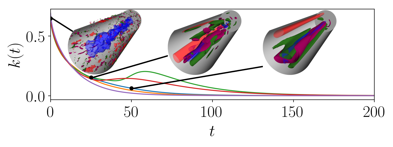
(b) 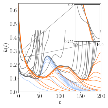 (c)
(c)
We utilize the Openpipeflow solver (Willis, 2017) to simulate pipe flow in an axially-periodic computational domain of length , where is the pipe radius. The Reynolds number is set to , where is the centerline velocity, is the kinematic viscosity, and the resolution is identical to the one used in Budanur & Hof (Budanur and Hof, 2018). In results, the time scale is chosen to be advective unit . In numerical simulations, a convenient method for obtaining initial conditions that have flatter mean profiles than normal levels at a certain Re is to take typical turbulent states from higher Re. Fig. 1 (a) shows the time-evolution of the perturbation kinetic energy of the velocity fluctuations with respect to the laminar flow, from five simulations at where we used typical turbulent states from as initial conditions. The flow structures visualized in fig. 1 correspond to three snapshots from one of the simulations and they illustrate the laminarization of the highly-turbulent initial state. We carried out edge-tracking starting with one of these states at . Let us denote it by . Fig. 1 (b) shows the time-evolution of the kinetic energy when initial conditions , with , evolve at . The time-series data on fig. 1 (b) was produced as follows: we first set and forward-integrated these initial conditions and observed that and laminarized while the initial condition with became turbulent. We then carried out two bisection searches, akin to that of ref. Itano and Toh (2001), for and such that simulations neither become turbulent nor laminarize. On fig. 1 (b), the time series data with initial conditions are shown orange while those with are plotted blue. As shown in the time-series plots, there appear to be two boundaries between the laminarizing trajectories and the ones that trigger turbulence. The low-energy boundary (blue) separates the initial conditions that are strong enough to trigger turbulence from those that are too weak. In contrast, the high-energy boundary (orange) separates the initial conditions that are too strong to trigger turbulence from those that are weak enough. We will refer this latter boundary as the upper edge of chaos. Both trajectories obtained from the bisection end up in the vicinity of the same edge state, characteristic of which are described by ref. Budanur and Hof (2018). In fig. 1 (c), we show a state-space sketch illustrating this numerical experiment, where the Euclidean distance from the laminar state should be interpreted as the square root of the perturbation energy and the stable and unstable manifolds of the edge state are annotated with and , respectively. The initial conditions of our numerical experiment lie along the dashed line in fig. 1 (c), and the high-energy intersection of this line with the stable manifold of the edge state marks the upper edge of chaos.
(a) 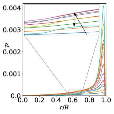 (b)
(b) 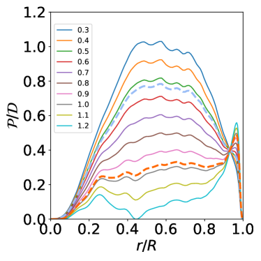
(c) 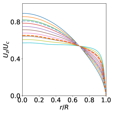 (d)
(d) 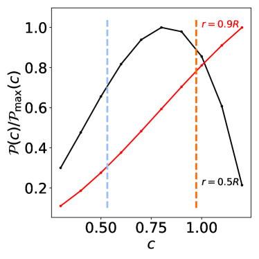
For high-energy turbulent initial conditions to laminarize, they must experience substantial energy losses. We are now going to examine where these losses take place by measuring turbulent energy production and dissipation as a function of the radial coordinate. When the turbulent velocity field is decomposed into its mean and fluctuating parts , rates of the turbulent energy production and the dissipation can be expressed as follows (Pope, 2000)
| (1) |
where is the fluctuating rates of strain tensor and . Hence, turbulent dissipation can also be expressed as
| (2) |
It can be readily seen from (2) that scaling up the amplitude of velocity fluctuations increases the dissipation everywhere. The production, on the other hand, has a different trend: as we have visualized in fig. 2 (a), scaling up the velocity fluctuations increases the production near the pipe wall (), however, away from the wall, this trend reverses. As a result, the bulk region of the pipe becomes completely dissipative as illustrated by the radial profiles of , shown in fig. 2 (b). This is due to the gradient term in the production equation (1) and flattening of the velocity profile for highly turbulent initial conditions as shown in fig. 2 (c). Figure 2(d) shows the normalized production at and as a function of the scaling coefficient . While the production near the wall increases monotonically with , the production in the bulk peaks in the range of that lead to transition, delimited by the vertical dashed blue (lower edge) and orange (upper edge) lines. For values of that lead to transition, the maximum of the normalized production is in the bulk region of the pipe, thus suggesting the importance of fluctuations away from the pipe wall for transition.
Open-loop control strategies that aim to laminarize turbulent flow, such as the ones employed by Kühnen et al. Kühnen et al. (2018), must achieve two goals: (1) manipulate the flow in such a way that its structures are dissipative at a given Re, (2) avoid retransition to turbulence. We hypothesize that the flattening of mean profile and resulting decrease of production in the bulk region ensures the second condition by eliminating all fluctuations in the bulk. As a first test of this hypothesis, we removed the mean of the axial velocity perturbations from the initial conditions on the laminarizing side of the upper edge, and rerun our numerical experiments. Albeit being energetically weaker, these initial conditions had velocity profiles equal to that of the laminar flow and they triggered the transition after an initial small energy drop. As a further test, we performed simulations with random solenoidal initial conditions that do not alter the mean profile. To this end, we populated a subset of modes in the spectral expansion of the velocity field (excluding the mean-flow distortion) with random amplitudes and ran the pressure solver on this state in order to ensure that it is divergence-free; see ref. Marensi et al. (2019) for details. Given they are strong enough, all initial conditions constructed this way lead to a transition to turbulence and we did not observe an upper edge of chaos in this case.
Turbulent wall-bounded shear flows are in equilibrium in a statistical sense. That is, on average, an equal amount of turbulent kinetic energy is produced and dissipated. It is well known (Pope, 2000; Kim et al., 1987; Yang et al., 2018) that the majority of the production takes place near the wall, where the shear is largest, and the flow becomes strongly dissipative away from the wall. The edge state of the pipe flow under consideration accommodates traveling wave solutions, which are not only statistically sustained but also dynamically invariant. In other words, they are in energy balance at all times. In the next section, we demonstrate that the energy budget of these lower-branch traveling waves or edge solutions is remarkably different from that of the turbulence, and the production away from the wall plays an essential role in sustaining them.
III Energetics of the edge state
The edge state of a shear flow is considered to be dynamically invariant, that is, if an initial condition starts exactly on the edge state, it should stay there forever. When the edge state is stationary (Itano and Toh, 2001), or time-periodic (Toh and Itano, 2003; Avila et al., 2013) this description can be supported by computing numerically exact invariant solution by a Newton method. When the edge state is chaotic as it is the case here, such a computation is not possible; and thus, the edge state can only be followed by edge tracking for finite times, as shown in fig. 1 (b). Even though the stable and unstable manifolds of chaotic sets are not well defined, the edge-tracking observations that are reported in the previous literature (Schneider et al., 2007; Duguet et al., 2008; Budanur and Hof, 2018) and the current work agree with the hypothesis that the edge state of the pipe flow is an invariant set of saddle-type. Moreover, refs. Duguet et al. (2008) and Budanur and Hof (2018) reported that edge tracking trajectories approach traveling waves of the pipe flow, which are by definition time-invariant. Fig. 3(a) shows the ratio as a function of radius for the traveling waves and , which are embedded in the laminar-turbulent boundary (Budanur and Hof, 2018). For the traveling waves and , the curve peaks at and respectively, which, is quite different from the turbulent case.
(a) 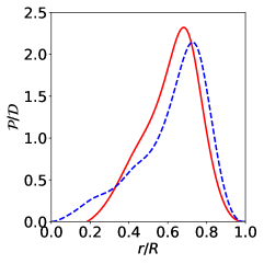 (b)
(b) 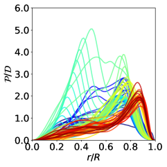 (c)
(c) 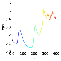
In order to see how generic trajectories on the laminar turbulent boundary are sustained, we measured along an edge-tracking trajectory, which proceeds towards turbulence after spending a long time on the laminar turbulent boundary. Fig. 3(b) shows the time-evolution of measured at instances separated by and the time is color-coded as in the time-series of fig. 3 (c). Once the turbulence is statistically stationary (, red curves on fig. 3(b)), the peak settles in the near-wall region (). Prior to this, when the trajectory is exploring the edge-state, has a completely different radial-profile with one or more maxima away from the wall. Similar to the traveling waves on the laminar-turbulent boundary, the chaotic edge state is also sustained by the production away from the wall.
IV Transition from the minimal seed
(a) 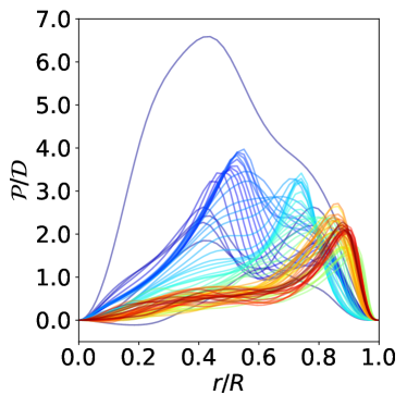 (b)
(b) 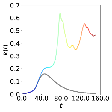
Refs. Pringle and Kerswell (2010); Pringle et al. (2012); Marensi et al. (2019) provided evidence that the nonlinear optimal in pipe flow tracks the laminar-turbulent boundary before either relaminarizing or triggering turbulence. We analyze the curves at different stages of the transition from the minimal seed in order to reveal the radial locations of the strong energy amplification.
We calculate the minimal seed at , with two-digits accuracy in the critical initial energy. Following previous studies (e.g. (Pringle et al., 2012)), an optimization horizon is chosen. Fig. 4(a) shows a family of curves along the minimal seed trajectory, separated by time intervals of and colored according to the coding given in fig. 4(b). The latter graph shows the time-series of the kinetic energy for the two initial conditions that bracket the minimal seed for transition, up to the chosen accuracy. Analogous to fig. 3(b), once the turbulent attractor is reached (red curves in fig. 4(a)) the peak of settles in the region close to the wall, while in the initial growth phase, up to the edge and when tracking the edge (blue curves in fig. 4(a)), the peak of is closer to the pipe center. Similar to the traveling waves embedded in the laminar-turbulent boundary and to the chaotic edge, the minimal seed is also strongly amplified in the bulk region. Fig. 4 thus supports our picture that the (large-scale) structures away from the the pipe wall are more important than the (small-scale) structures close to the wall for the transition process, while, after turbulence is triggered, the near-wall structures become dominant.
Particularly interesting is the significant increase of experienced by the minimal seed during its initial evolution, up to the edge; e.g. refer to the blue curve almost reaching in fig. 4. To better understand the initial mechanism of growth of the minimal seed, we closely analyze the profiles in the time window . Figs. 5(a, b) show a zoom of figs. 4(a, b) in this time window, with intervals of . The time evolution of the peak of the production to dissipation ratio and of its radial position are shown in figure 5(c). As outlined in §I, in the Orr and oblique-wave phases of its initial evolution, the minimal seed gradually delocalizes and undergoes most of its energy growth. This is clearly seen in figure 5(c) by the marked increase of and by the shift of towards the pipe center. The peak is reached at and occurs almost at . After this initial spurt of energy and delocalization, approaches the typical ‘turbulent’ value of (Pope, 2000) and moves closer to the wall, i.e. . Marensi et al. (2019) showed that the minimal seed at the end of the Orr and oblique-wave phases of its evolution is a useful tool to measure transition thresholds for typical ambient disturbances. The Orr process ( for ) was identified by analyzing the flow topology of the minimal seed at the very initial stage of its evolution, but, as pointed out by the authors themselves, there was some discretion in the identification of this phase. The oblique-wave phase ( for the same range of ) is usually signaled by a ‘bump’ in the time evolution of the three dimensional energy , i.e. the energy associated with the streamwise dependent modes only. However, in a long pipe this ‘bump’ is obscured by the long wave-length modes, which thus need to be filtered out first. Here, while analyzing the energetics of transition in pipe flow, we realized that the Orr and oblique-wave phases of the transition from the minimal seed could be identified in a much easier and clearer way using the curves of . In particular, a graph like that shown in figure 5(c), indicates that the Orr phase ends at where reaches its peak, while the end of the oblique-wave phase is signaled by the jump of from close to the pipe center to close to the wall (and, correspondingly, the marked change of slope of ) which occurs at . The analysis of the profiles is thus found to provide a simple and clear method for identifying the Orr and oblique-wave phases of the minimal seed evolution.
V Implications for flow control
(a) 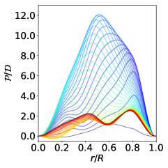 (b)
(b) 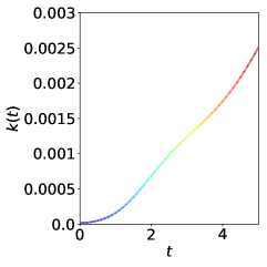 (c)
(c) 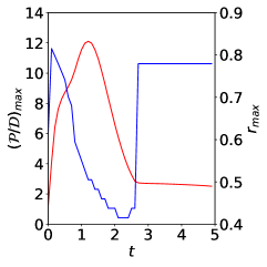
(a) 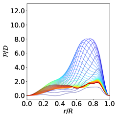 (b)
(b) 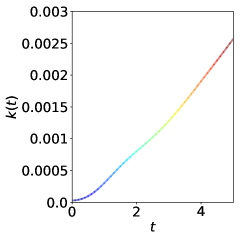 (c)
(c) 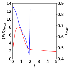
Marensi et al. Marensi et al. (2019) showed that flattening the base profile in a pipe flow not only destabilizes the turbulence, as in the experiment of Kühnen et al. Kühnen et al. (2018), but it also enhances the nonlinear stability of the laminar flow. Minimal seed calculations were performed with a flattened base profile (Kühnen et al., 2018), namely
| (3) |
where is the centerline difference between the laminar profile and the target profile and is set by the constant mass flux condition. The critical initial energy of the minimal seed was found to increase with increasing values of , that is, the flattening expands the basin of attraction of the laminar state. Here, we analyze this phenomenon in the light of the profiles and of their time evolution. For example, an interesting question is the following: which of the phases of the minimal seed amplification is the flattening of the base profile affecting and how? First, we repeat the minimal seed calculation of ref. Marensi et al. (2019) for and at . The corresponding curves are shown in fig. 6. By comparing it with fig. 5, we observe that the production in the bulk region is strongly reduced by the flattening. Fig. 6 also shows that all three phases of the minimal seed amplification are still present in the forced case, but they are not able to achieve as much energy production as in the unforced case (for example in the Orr phase, the peak is almost lower than with the parabolic base profile.). These observations illustrate that strategies to delay transition have to take the central part of the flow into account. Since transition relies on the production away from the wall, a flatter velocity profile effectively reduces the susceptibility of the flow to perturbations.
VI Conclusion
In this paper, we demonstrated that in pipe flow at the transitional stages, velocity field fluctuations are amplified away from the wall as opposed to the typical turbulent fluctuations, which are predominantly generated near the wall . To this end, we numerically investigated various transition scenarios including the perturbations that are too energetic to initiate turbulence (the upper edge) and the perturbations that are only energetic enough (the minimal seeds) for the transition. In all cases, we observed that the strong energy amplification away from the wall is an essential stage of transition.
Although we focused here on the production and dissipation terms for our diagnostics, it should be noted that the full energy balance equation of the pipe flow also have pressure, viscous, and nonlinear transport terms Pope (2000). For the highly-turbulent initial conditions we studied in Section II, we found these terms to be negligible in the bulk region. For the traveling waves and other snapshots from the edge state, while the pressure transport was still very small, the viscous and nonlinear terms had peaks located close to that of the production. This trend is also observed in the turbulent channel flow Pope (2000) when these terms are evaluated as a function of the wall-normal coordinate and interpreted as the redistribution of excess energy due to production peak. We believe that our case here is similar since the edge state is dynamically invariant and, thus, it must exhibit energy balance.
In both transitions from the edge state (fig. 3) and from the minimal seeds (figs. 4–6), kinetic energy of the velocity perturbations show episodes of strong amplification. Notice that all of the corresponding curves have values greater than in the bulk of the domain. This is expected since the volume integral of gives the instantaneous change in total kinetic energy of the velocity fluctuations.
During the transition from the minimal seed, the peak of and its radial location have proven to be a clear indicator of which state of transition is taking place. Such knowledge is of great importance when investigating the nonlinear stability of shear flows in subcritical transition scenarios as it gives insights on which growth mechanism to target in order to enhance or suppress transition.
In many industrial applications, turbulence is undesirable due to its high energy cost. Our results indicate that the control strategies, which aim to avoid transition must eliminate fluctuations away from the pipe wall. Furthermore, ref. Kühnen et al. (2018) measured transient growth due to the non-normality of the linearized Navier-Stokes operator assuming the mean profile to be the base flow. They found that the transient growth was substantially suppressed when the profile was flattened. Our results suggest that the transient growth of the mean profile serves as a proxy of the production away from the wall, which is necessary for the transition to turbulence.
References
- Reynolds (1883) O. Reynolds, “An experimental investigation of the circumstances which determine whether the motion of water shall be direct or sinuous, and the law of resistance in parallel channels,” Proc. Roy. Soc. Lond. Ser A 174, 935–982 (1883).
- Skufca et al. (2006) J. D. Skufca, J. A. Yorke, and B. Eckhardt, “Edge of Chaos in a parallel shear flow,” Phys. Rev. Lett. 96, 174101 (2006).
- Hopf (1948) E. Hopf, “A mathematical example displaying features of turbulence,” Commun. Pure Appl. Math. 1, 303–322 (1948).
- Alligood et al. (1997) K. T. Alligood, T. D. Sauer, and J. A. Yorke, “Stable manifolds and crises,” in Chaos: An Introduction to Dynamical Systems (Springer Berlin Heidelberg, Berlin, Heidelberg, 1997) pp. 399–445.
- Grebogi et al. (1982) C. Grebogi, E. Ott, and J. A. Yorke, “Chaotic attractors in crisis,” Phys. Rev. Lett. 48, 1507–1510 (1982).
- Grebogi et al. (1983) C. Grebogi, E. Ott, and J. A. Yorke, “Crises, sudden changes in chaotic attractors, and transient chaos,” Physica D 7, 181–200 (1983).
- Itano and Toh (2001) T. Itano and S. Toh, “The dynamics of bursting process in wall turbulence,” J. Phys. Soc. Japan 70, 701–714 (2001).
- Toh and Itano (2003) S. Toh and T. Itano, “A periodic-like solution in channel flow,” J. Fluid Mech. 481, 67–76 (2003).
- Schneider et al. (2007) T. M. Schneider, B. Eckhardt, and J. Yorke, “Turbulence, transition, and the edge of chaos in pipe flow,” Phys. Rev. Lett. 99, 034502 (2007).
- Schneider et al. (2008) T. M. Schneider, J. F. Gibson, M. Lagha, F. De Lillo, and B. Eckhardt, “Laminar-turbulent boundary in plane Couette flow,” Phys. Rev. E. 78, 037301 (2008), arXiv:0805.1015.
- Mellibovsky et al. (2009) F. Mellibovsky, A. Meseguer, T. M. Schneider, and B. Eckhardt, “Transition in localized pipe flow turbulence,” Phys. Rev. Lett. 103, 054502 (2009).
- Schneider et al. (2010) T. M. Schneider, D. Marinc, and B. Eckhardt, “Localized edge states nucleate turbulence in extended plane Couette cells,” J. Fluid Mech. 646, 441–451 (2010).
- Zammert and Eckhardt (2014) S. Zammert and B. Eckhardt, “A spotlike edge state in plane Poiseuille flow,” PAMM 14, 591–592 (2014).
- Khapko et al. (2016) T. Khapko, T. Kreilos, P. Schlatter, Y. Duguet, B. Eckhardt, and D. S. Henningson, “Edge states as mediators of bypass transition in boundary-layer flows,” J. Fluid Mech. 801 (2016), 10.1017/jfm.2016.434.
- Budanur and Hof (2018) N. B. Budanur and B. Hof, “Complexity of the laminar-turbulent boundary in pipe flow,” Phys. Rev. Fluids 3, 054401 (2018).
- Pringle and Kerswell (2010) C. C. T. Pringle and R. R. Kerswell, “Using nonlinear transient growth to construct the minimal seed for shear flow turbulence,” Phys. Rev. Lett. 105, 154502 (2010).
- Pringle et al. (2012) C. C. T. Pringle, A. P. Willis, and R. R. Kerswell, “Minimal seeds for shear flow turbulence: using nonlinear transient growth to touch the edge of chaos,” J. Fluid Mech. 702, 415–443 (2012).
- Duguet et al. (2013) Y. Duguet, A. Monokrousos, L. Brandt, and D. S. Henningson, “Minimal transition thresholds in plane Couette flow,” Physics of Fluids 25, 084103 (2013).
- Cherubini and Palma (2014) S. Cherubini and P. De Palma, “Minimal perturbations approaching the edge of chaos in a couette flow,” Fluid Dyn. Res 46, 041403 (2014).
- Kerswell et al. (2014) R. R. Kerswell, C. C. T. Pringle, and A. P. Willis, “An optimization approach for analysing nonlinear stability with transition to turbulence in fluids as an exemplar,” Rep. Progr. Phys. 77, 085901 (2014).
- Marensi et al. (2019) E. Marensi, A. P. Willis, and R. R. Kerswell, “Stabilisation and drag reduction of pipe flows by flattening the base profile,” J. Fluid Mech. 863, 850–875 (2019).
- Joseph and Hung (1971) D. D. Joseph and W. Hung, “Contributions to the nonlinear theory of stability of viscous flow in pipes and between rotating cylinders,” Arch. Rational Mech. Anal. 44, 1–22 (1971).
- Kühnen et al. (2018) J. Kühnen, B. Song, D. Scarselli, N. B. Budanur, M. Riedl, A. P. Willis, M. Avila, and B. Hof, “Destabilizing turbulence in pipe flow,” Nat. Phys. 14, 386–390 (2018).
- Willis (2017) A. P. Willis, “The Openpipeflow Navier–Stokes solver,” SoftwareX 6, 124–127 (2017).
- Pope (2000) S. B. Pope, Turbulent Flows (Cambridge Univ. Press, Cambridge, 2000).
- Kim et al. (1987) J. Kim, P. Moin, and R. Moser, “Turbulence statistics in fully developed channel flow at low Reynolds number,” J. Fluid Mech. 177, 133–166 (1987).
- Yang et al. (2018) Q. Yang, A. P. Willis, and Y. Hwang, “Energy production and self-sustained turbulence at the kolmogorov scale in couette flow,” J. Fluid Mech. 834, 531–554 (2018).
- Avila et al. (2013) M. Avila, F. Mellibovsky, N. Roland, and B. Hof, “Streamwise-localized solutions at the onset of turbulence in pipe flow,” Phys. Rev. Lett. 110, 224502 (2013).
- Duguet et al. (2008) Y. Duguet, A. P. Willis, and R. R. Kerswell, “Transition in pipe flow: the saddle structure on the boundary of turbulence,” J. Fluid Mech. 613, 255–274 (2008), arXiv:0711.2175.