A well-balanced finite difference WENO scheme
for shallow water flow model

Abstract

In this paper, we are concerned with shallow water flow model over non-flat bottom topography by high-order schemes. Most of the numerical schemes in the literature are developed from the original mathematical model of the shallow water flow. The novel contribution of this study consists in designing an finite difference weighted essentially non-oscillatory (WENO) scheme based on the alternative formulation of the shallow water flow model, denoted as “pre-balanced” shallow water equations and introduced in {Journal of Computational Physics 192 (2003) 422-451}. This formulation greatly simplifies the achievement of the well-balancing of the present scheme. Rigorous numerical analysis as well as extensive numerical results all verify that the current scheme preserves the exact conservation property. It is important to note that this resulting scheme also maintains the non-oscillatory property near discontinuities and keep high-order accuracy for smooth solutions at the same time.

1 Introduction

In this paper, we are interested in numerical simulation for the shallow water flow model by high order finite difference schemes. The governing equations, referred to as the shallow water equations, have a wide applications in hydraulic and coastal engineering [1, 2]. Some effects, such as friction on the bottom topography, wind forces, as well as variations of the channel width, can result in additional source terms to the governing equations. Herein, we only consider the geometrical source term due to the non-flat bottom topography. The one-dimensional case has the following form

$$\left\{\begin{array}[]{l}h_{t}+(hu)_{x}=0,\\ (hu)_{t}+\left(hu^{2}+\frac{1}{2}gh^{2}\right)_{x}=-ghb_{x},\end{array}\right.$$ (1)

where $h$ and $u$ are the water depth and the depth-averaged water velocity, respectively, $g$ is the gravitational constant, and $b$ stands for the bottom topography. Therefore, $H=h+b$ denotes the water surface level and $hu$ represents the water discharge.

Shallow water equations with source terms are also called as balance laws. Balance laws often admit steady state solution in which the source term is exactly balanced by the non-zero flux gradient. Thus it is desirable to maintain the balance at the discrete level, but such balance are usually neither a constant nor a polynomial function. For most numerical schemes, the truncation error between the flux gradient and the source term is not exactly zero for the above balance. So the numerical schemes for the shallow water equations with the source term is a challenging task with the presence of the source term. There are a lot of efforts focused on this subject in the literature, see e.g., [3, 4, 5]. Bermudez and Vazquez [6] firstly proposed the idea of “exact conservation property” (exact C-property), which means that a scheme is exactly compatible with the still water stationary solution

$$h+b=\mathrm{constant}\;\;and\;\;u=0.$$ (2)

This property is necessary for the balance between the flux gradient and the source term and is also known as well balancing. An efficient scheme should satisfies this property. Such schemes are often regarded as well-balanced schemes after the pioneering works of Greenberg et al. [7, 8] and the study for the well-balanced schemes is currently a very active subject of research. The important advantages of well-balanced schemes over non-well-balanced schemes is that they can accurately resolve small perturbations of such steady state solution with relatively coarse meshes [9, 10]. However, straightforward treatments to the source term can not preserve the exact C-property and even leads to unacceptable numerical results such as spurious numerical oscillations. To construct well-balanced schemes, there are many attempts to handle the geometric source term. LeVeque [11] brought forward a high-resolution Godunov-type finite volume scheme by a quasi-steady wave-propagation algorithm. Zhou et al. [12] designed a robust well-balanced scheme based on a Godunov-type method and a surface gradient method for the data reconstruction. By the aid of a special decomposition of the source term, Xing and Shu [13] developed a high order well-balanced finite difference weighted non-oscillatory (WENO) schemes. Furthermore, Xing and Shu [14, 15, 16] extended their idea and designed well-balanced finite volume WENO schemes and discontinuous Galerkin (DG) finite element methods for a class of balance laws equations. Audusse et al. [17, 18] designed a fast well-balanced scheme by a hydrostatic reconstruction procedure. With the help of a new quadrature formula for the source term, Noelle et al. [19] designed well-balanced finite volume WENO schemes with arbitrary order of accuracy. Caleffi [20] for the first time extended the Hermite WENO schemes [21] to the shallow water equations and obtained a well-balanced schemes even with the source term. More recently, Hou et al. [22] proposed a robust well-balanced well-balanced cell-centered finite volume method on unstructured grids. More information about well-balanced schemes can be found in the lecture note [9].

Most of the numerical schemes reviewed above are developed considering as a starting mathematical model the shallow water equations in their classical form. An alternative formulation of the shallow flow model, denoted as “pre-balanced” shallow water equations, was introduced by Roges et al. in [23] to the aim of simplify the achievement of the well-balancing. The new formulation was obtained assuming as dependent variable the water elevation instead of the water depth and by a simple analytical manipulation. This formulation was adopted to develop different numerical schemes. For example in [24] the pre-balanced shallow water equations are integrated combining the PRICE-C method with a path-conservative method while in [25] the same equations are integrated by a well-balanced central WENO scheme.

The original contribution of this research consists in an upwind finite difference scheme based on the pre-balanced shallow water flow model [23]. In analogy to [23], this new formulation greatly simplifies the achievement of exact C-property of the present scheme. Rigorous numerical analysis as well as extensive benchmark examples all verify the satisfaction of the exact C-property of the resulting scheme. In addition, the high-order accuracy is obviously obtained at the same time.

This paper is organized as follows: in Section 2, we give a brief review of the finite difference WENO schemes. We propose a high order well-balanced finite difference WENO scheme in Section 3 based on an equivalent governing equations for the shallow water flow model. Numerical experiments of one- and two-dimensional cases are carried out in Section 4.1 and Section 4.2, respectively. Conclusions are given in Section 5.

2 A review of finite difference WENO schemes

The first finite difference WENO scheme was designed in 1996 by Jiang and Shu [26] for one- and two-dimensional hyperbolic conservation laws. More detailed information of WENO schemes can be found in the lecture note [27]. For the latest advances regarding WENO schemes, we refer to the review [28]. We begin with the description for the one-dimensional scalar conservation laws

$$u_{t}+f(u)_{x}=0.$$ (3)

For simplicity, we assume that the grid points $\{x_{j}\}$ are uniform. We define the cell size and cells by $\Delta x=x_{j+1}-x_{j}$ and $I_{j}=[x_{j-1/2},x_{j+1/2}]$ with $x_{j+1/2}=x_{j}+\Delta x/2$, respectively. A semidiscrete conservative high order finite difference scheme of (3) can be formulated as follows

$$\frac{{\rm d}u_{j}(t)}{{\rm d}t}=-\frac{1}{\Delta x}\left(\hat{f}_{j+1/2}-\hat{f}_{j-1/2}\right),$$ (4)

where $u_{j}(t)$ is the numerical approximation to the point value $u(x_{j},t)$, and the numerical flux $\hat{f}_{j+1/2}$ is used to approximate $h_{j+1/2}=h\left(x_{j+1/2}\right)$ with high order accuracy. Here $h(x)$ is implicitly defined as in [26]

$$f(u(x))=\frac{1}{\Delta x}\int^{x+\Delta x/2}_{x-\Delta x/2}h(\xi)d\xi.$$

We take upwinding into account to maintain the numerical stability and split a general flux into two parts either globally or locally

$$f(u)=f^{+}(u)+f^{-}(u),$$

where $\displaystyle\frac{{\rm d}f^{+}(u)}{{\rm d}u}\geq 0$ and $\displaystyle\frac{{\rm d}f^{-}(u)}{{\rm d}u}\leq 0$. With respect to $f^{+}(u)$ and $f^{-}(u)$, we can get numerical fluxes $\hat{f}^{+}_{j+1/2}$ and $\hat{f}^{-}_{j+1/2}$ using the WENO reconstruction, respectively. The computation of $\hat{f}^{+}_{j+1/2}$ and $\hat{f}^{-}_{j+1/2}$ is described in A. Finally, we get the numerical fluxes as follows

$$\hat{f}_{j+1/2}=\hat{f}^{+}_{j+1/2}+\hat{f}^{-}_{j+1/2}.$$

With numerical fluxes $\hat{f}_{j+1/2}$ at hand, we can write the semidiscrete scheme (4) as an ordinary differential equation (ODE) system

$$u_{t}=L(u).$$

Eventually, we discretize this ODE system in time by the third-order total variation diminishing (TVD) Runge-Kutta method [29]

$$\begin{array}[]{lcl}u^{(1)}&=&u^{n}+\Delta tL\left(u^{n}\right),\\ u^{(2)}&=&\frac{3}{4}u^{n}+\frac{1}{4}u^{(1)}+\frac{1}{4}\Delta tL\left(u^{(1)}\right),\\ u^{n+1}&=&\frac{1}{3}u^{n}+\frac{2}{3}u^{(2)}+\frac{2}{3}\Delta tL\left(u^{(2)}\right).\end{array}$$ (5)

3 The numerical scheme

In this section, we design a well-balanced finite difference WENO scheme for the shallow water flow model. For the sake of simplicity, we take the one-dimensional case as an example.

Herein, we apply the equivalent governing equations as in [23], where the water surface level $H$ instead of the water depth $h$ as an unknown variable since the bottom topography b is independent of the time $t$ and the physical fluxes have been changed accordingly. Similar procedure is also used in the surface gradient method by Zhou et al. [12], the centered scheme of Canestrelli et al. [24], the discontinuous Galerkin finite element methods of Kesserwani and Liang [30], and the central WENO scheme of Li et al. [25].

Equivalent to the original governing equations (1), we apply the following ones as in [23],

$$\left\{\begin{array}[]{l}H_{t}+(hu)_{x}=0,\\ (hu)_{t}+\left(\displaystyle\frac{(hu)^{2}}{H-b}+\frac{1}{2}gH^{2}-gHb\right)_{x}=-gHb_{x},\end{array}\right.$$ (6)

which can be denoted by a compact vector form

$$U_{t}+f(U)_{x}=S,$$

where $U=(H,\;hu)^{T},\;f(U)=\left(\displaystyle hu,\;\frac{(hu)^{2}}{H-b}+\frac{1}{2}gH^{2}-gHb\right)^{T},\;\mbox{and}\;S=(0,\;-gHb_{x})^{T}.$

In this paper, we are intent on solving the equivalent governing equations (6) by linear schemes. For a given linear scheme, all the spatial derivatives are approximated by a linear finite difference operator $D$ that satisfyies

$$D(\alpha f_{1}+\beta f_{2})=\alpha D(f_{1})+\beta D(f_{2})$$ (7)

for constants $\alpha,\;\beta$ and any grid functions $f_{1},\;f_{2}$. For such linear schemes, we have

Proposition 1.

For the still water stationary solution (2), linear schemes satisfying (7) for the shallow water equations (6) maintain the exact C-property.

Proof.

For still water stationary solution (2), any consistent linear schemes satisfying (7) are exact for the first equation $(hu)_{x}=0$ due to $u=0$. For the second one, with a given linear finite difference operator $D$, the error between the flux gradient and the source term reduces to

$$\begin{array}[]{l}D\left(\displaystyle\frac{(hu)^{2}}{H-b}+\frac{1}{2}gH^{2}-gHb\right)+gHD(b)\\ =D\left(\frac{1}{2}gH^{2}-gHb+gHb\right)\\ =D\left(\frac{1}{2}gH^{2}\right)\\ \equiv 0,\end{array}$$

here the first equality is due to the linearity of $D$, $u=0$ and $H=h+b=constant$; the second equality is just a simple algebra operation inside the parenthesis, and the last one is again due to the fact that $H=h+b=constant$ and the consistency of the operator $D$. This completes the proof. ∎

Unfortunately, the finite difference WENO schemes described in Section 2 are nonlinear. The nonlinearity comes from the nonlinear weights, which in turn come from the nonlinearity of the smoothness indicators. In order to construct a linear scheme which can maintain the exact C-property even with the presence of the nonlinearity of the nonlinear weight, we adopt the following procedures. The resulting scheme maintains the exact C-property and the accuracy is not affected.

Firstly, we compute the numerical flux $\hat{f}_{j+1/2}$ to approximate the flux gradient $f(U)_{x}$. For similarity, we consider a finite difference WENO scheme with a global Lax-Friedrichs flux splitting, denoted by WENO-LF scheme. Now the physical flux $f(U)$ is written out as

$$f(U)=f^{+}(U)+f^{-}(U),$$

where

$$f^{\pm}(U)=\frac{1}{2}\left[\left(\begin{array}[]{c}hu\\ \displaystyle\frac{(hu)^{2}}{H-b}+\frac{1}{2}gH^{2}-gHb\end{array}\right)\pm\alpha_{i}\left(\begin{array}[]{c}H\\ hu\end{array}\right)\right],$$ (8)

with

$$\alpha_{i}=\max\limits_{u}\big{|}\lambda_{i}(u)\big{|},$$ (9)

here $\lambda_{i}(u)$ being the $i$th eigenvalue of the Jacobian matrix $f^{\prime}(U)$.

Moreover, in order to achieve better numerical results at the price of more complicated computations, the WENO reconstruction is always accompanied by a local characteristic decomposition procedure [27], which is more robust than a component-wise version.

Subsequently, we will verify that for the still water stationary solution (2), the present WENO scheme is a linear scheme. We refer to B for the complete verification of the linearity of the present scheme. Consequently, we have the following result according to the Proposition 1.

Proposition 2.

For the still water stationary solution (2), the WENO-LF scheme as stated above for the shallow water equations (6) maintains the exact C-property and their original accuracy.

4 Numerical results

In this Section, we carry out extensive one- and two-dimensional numerical experiments to demonstrate the performances of a fifth-order ($r=2$) finite difference WENO scheme. In all the numerical examples, time discretization is by the classical third-order Runge-Kutta method [29]. The $CFL$ number is taken as $0.6$, except for the accuracy tests where smaller time step is taken to ensure that spatial errors dominate. The gravitation constant g is taken as $9.812\,\mbox{m}/\mbox{s}^{2}$.

4.1 One-dimensional cases

Firstly, we present numerical results of our fifth-order finite difference WENO-LF scheme for the one-dimensional model (6).

4.1.1 Testing the exact C-property

We verify the exact C-property of the resulting scheme by the following test cases in [13] over two different bottom topographies on a computational domain $[0,10]$. The first bottom topography is smooth

$$b(x)=5e^{-\frac{2}{5}(x-5)^{2}},$$

and the second one is discontinuous

$$b(x)=\left\{\begin{array}[]{ll}4&\mathrm{if}\;4\leq x\leq 8,\\ 0&\mathrm{otherwise}.\end{array}\right.$$

The initial data is the still water stationary solutions

$$h+b=10\;\;\mbox{and}\;\;u=0.$$

We compute the solution up to $t=0.5$ s on a mesh with $200$ uniform cells. In order to show that the exact C-property is maintained even with round off error, we apply single, double and quadruple precisions, respectively, to carry out the computation. We present the $L^{1}$ and $L^{\infty}$ error for $h$ and $hu$ in Tables 2 and 3 for the two different bottom topographies. We can clearly observe that the $L^{1}$ and $L^{\infty}$ errors are all at the level of round off error for different precisions, and verify the expected exact C-property accordingly.

4.1.2 Testing the orders of accuracy

In this test case, we test the fifth-order accuracy of the scheme for the smooth solution. We apply the following bottom topography and the initial condition

$$b(x)=\sin^{2}(\pi x),\;h(x,0)=5+e^{\cos(2\pi x)},\;(hu)(x,0)=\sin(\cos(2\pi x)),\;x\in[0,1]$$

with periodic boundary conditions. We compute the test case up to $t=0.1$ s and apply the same fifth-order WENO scheme with $6400$ cells to obtain a reference solution. In Table 1, we list the $L^{1}$ errors and orders of accuracy for $h$ and $hu$. It is clear that we get the expected fifth-order accuracy for this test case. Due to the space limitation, we do not present the $L^{\infty}$ errors and the orders of accuracy, since they are similar with the $L^{1}$ errors and the orders of accuracy.

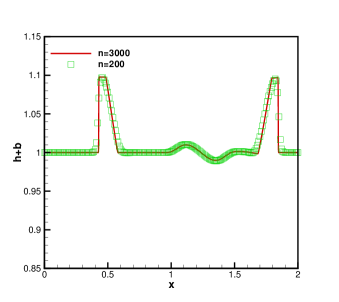
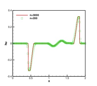
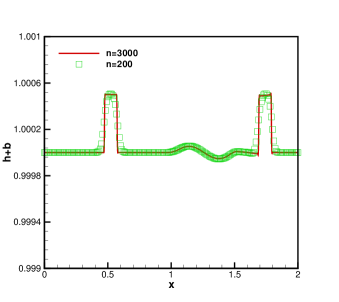
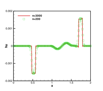
4.1.3 A small perturbation of a steady state water flow

The following quasi-stationary test case was proposed by LeVeque [11]. It is chosen to demonstrate the capability of the present scheme for the computation on a rapidly varying flow over a smooth bottom topography and the perturbation of a stationary state flow. The bottom topography consists of a bump

$$b(x)=\left\{\begin{array}[]{ll}0.25\left(\cos(10\pi(x-1.5))+1\right)&\mbox{if}\;1.4\leq x\leq 1.6,\\ 0&\mathrm{otherwise},\end{array}\right.$$

and the initial condition is given as

$$h(x,0)=\left\{\begin{array}[]{ll}1-b(x)+\epsilon&\mbox{if}\;1.1\leq x\leq 1.2,\\ 1-b(x)&\mathrm{otherwise},\end{array}\right.\;\mathrm{and}\;u(x,0)=0.$$

where $\epsilon$ is a non-zero perturbation constant. Two cases are considered: $\epsilon=0.2$ m (big pulse) and $\epsilon=0.001$ m (small pulse).

We present the water surface level $h+b$ and the water discharge $hu$ at $t=0.2$ s against reference solutions in Figs. 1 and 2 for the big pulse and the small pulse cases, respectively. The numerical results are resolved accurately, free of spurious numerical oscillations, and look very comparable to those found in the other existing literature.

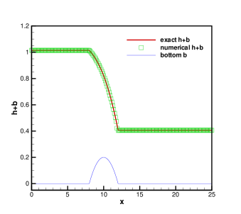
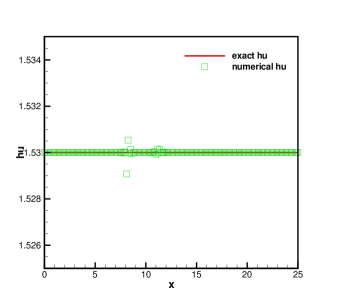
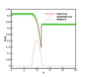
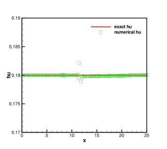
4.1.4 Steady flow over a hump

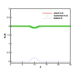
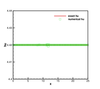
In this example, we employ three established benchmark test cases [3] with different boundary conditions. These test cases involve transcritical, supercritical and subcritical flows, respectively, in a $25$ m channel over a bump

$$b(x)=\left\{\begin{array}[]{ll}0.2-0.05(x-10)^{2}&\mathrm{if}\;8\leq x\leq 12,\\ 0&\mathrm{otherwise}.\end{array}\right.$$

The initial data are defined by

$$h(x,0)=0.33\;\;\mbox{and}\;\;u(x,0)=0.$$

We employ same computational parameters for the following three cases: uniform mesh with $200$ cells, final time $t=200$ s. Exact solutions for the three cases can be found in [31].

Case 1: Transcritical flow without a shock

A unit discharge of $1.53$ $\mbox{m}^{2}$/s is imposed at the upstream boundary, and the open boundary conditions ($du/dx=0$) are applied at the downstream one. We present the water surface level $h+b$ and the water discharge $hu$ in Fig.  3. It is obvious that the numerical solutions are very good agreement with the exact ones.

Case 2: Transcritical flow with a shock

A unit discharge of $0.18$ $\mbox{m}^{2}/\mbox{s}$ is imposed on the upstream boundary and a depth of $0.33$ m is imposed on the downstream boundary. We show the water surface level $h+b$ and the water discharge $hu$ against exact solutions in Fig.  4. The numerical results are free of spurious oscillations, which verifies the essentially non-oscillatory property of the current scheme.

Case 3: Subcritical flow

A unit discharge of $4.42$ $\mbox{m}^{2}/\mbox{s}$ is imposed on the upstream boundary and a depth of $2$ m is imposed on the downstream boundary. The numerical results are compared with exact solutions in Fig.  5, and very good agreement is achieved.

4.1.5 The dam break problem over a rectangular bump

This test case was used in [32]. Herein, we simulate a dam break problem over a rectangular bump, which involves a rapidly varying water flow over a discontinuous bottom topography. The bottom topography contains a rectangular bump:

$$b(x)=\left\{\begin{array}[]{ll}8&\mbox{if}\;\big{|}x-750\big{|}\leq 1500/8,\\ 0&\mathrm{otherwise}.\end{array}\right.$$

The initial conditions are given as follows

$$h(x,0)=\left\{\begin{array}[]{ll}20-b(x)&\mbox{if}\;x\leq 750,\\ 15-b(x)&\mathrm{otherwise},\end{array}\right.\;\mathrm{and}\;\;u(x,0)=0.$$

We present numerical results against reference solutions in Fig.  6, which indicate that the numerical results keep the essentially non-oscillatory property and are in good agreement with the reference solutions.

4.1.6 The tidal wave flow

This example was used in [33], in which almost exact solutions (a very good asymptotically derived approximation) were given. The bottom topography is defined as

$$b(x)=10+\frac{40x}{L}+10\sin\left(\pi\left(\frac{40x}{L}-\frac{1}{2}\right)\right),$$

with $L=14,000$ m being the channel length. Herein, we take the following initial conditions

$$h(x,0)=60.5-b(x),\;\;hu(x,0)=0,$$

and boundary conditions

$$h(0,t)=64.5-4\sin\left(\pi\left(\frac{4t}{86,400}+\frac{1}{2}\right)\right),\;\;hu(L,t)=0.$$

By means of the asymptotic analysis in [33], we can obtain the following almost exact solutions

$$h(x,t)=64.5-b(x)-4\sin\left(\pi\left(\frac{4t}{86,400}+\frac{1}{2}\right)\right),$$

$$hu(x,t)=\frac{(x-L)\pi}{5400}\cos\left(\pi\left(\frac{4t}{86,400}+\frac{1}{2}\right)\right).$$

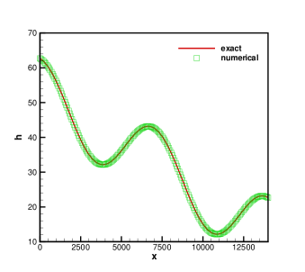
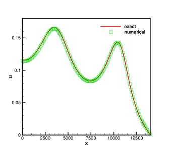
We compute the example on a mesh with $200$ uniform cells up to $t=7552.13$ s and present numerical results against exact solutions in Fig.  7, which strongly suggests that the numerical results are in good agreement with the exact ones.

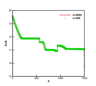
4.1.7 $1$-rarefaction and $2$-shock problem

Then we consider a example over a step bottom topography [34] to further test our scheme. The bottom topography consists of a step

$$b(x)=\left\{\begin{array}[]{ll}0&\mathrm{if}\;x\leq 0,\\ 1&\mathrm{otherwise},\end{array}\right.$$

on a computational domain $[-10,10]$, and the initial data are as follows

$$h(x,0)=\left\{\begin{array}[]{ll}4&\mbox{if}\;x\leq 0,\\ 1&\mbox{otherwise},\end{array}\right.\;\;u(x,0)=0.$$

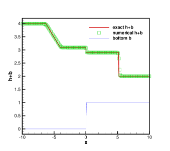
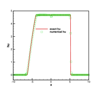
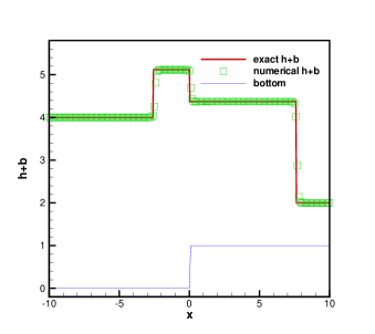
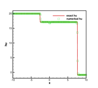
This test case produces a $1$-rarefaction spreading to the left and a $2$-shock traveling to the right. We illustrate the water surface level $h+b$ and the water discharge $hu$ at $t=1$ s against exact solutions in Fig.  8. We can clearly observe that the numerical results keep a sharp discontinuity transition.

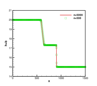
4.1.8 $1$-shock and $2$-shock problem

This test case is also over the same step bottom topography as in Section 4.1.7 on a computational domain $[-10,10]$. The initial data are given by

$$h(x,0)=\left\{\begin{array}[]{ll}4&\mbox{if}\;x\leq 0,\\ 1&\mathrm{otherwise},\end{array}\right.\;\mathrm{and}\;\;u(x,0)=\left\{\begin{array}[]{ll}5&\mathrm{if}\;x\leq 0,\\ -0.9&\mathrm{otherwise}.\end{array}\right.$$

This test case produces two shocks: the first one moving to the left and the second one to the right. We present the water surface level $h+b$ and the water discharge $hu$ at $t=1$ s against exact solutions in Fig.  9. It is evident that the numerical results possess a good resolution and are almost free of spurious numerical oscillations.

Remark 1.

As can be seen in Figs. 8 and 9, there are some minor numerical oscillations for the water discharge. The occurrence is mainly due to the non-flat bottom topography which can not be handled since the imbalance between the flux gradient and the source term as well as the moving water flow [35]. As the correct capturing of the water discharge is more difficult than the water surface level, so we are satisfied with the present numerical results. Although the current numerical scheme is well-balanced for the still water stationary solution, it is not able to maintain such a desirable exact C-property for the moving steady-state problem. Therefore, from Figs. 8 and 9, we can observe disturbance to discharge in those areas with abrupt change of the bottom topography and the water depth, which is a common phenomenon also predicted by other well-balanced schemes (e.g., [12, 23]). The disturbance is then advected by the flow as a wave and reaches the location as indicated in Figs. 8 and 9.

4.2 Two-dimensional cases

Subsequently, we consider two-dimensional cases. In analogy with the one-dimensional case, the governing equations are as follows

$$\left\{\begin{array}[]{l}H_{t}+(hu)_{x}+(hv)_{y}=0,\\ (hu)_{t}+\left(\displaystyle\frac{(hu)^{2}}{H-b}+\frac{1}{2}gH^{2}-gHb\right)_{x}+(huv)_{y}=-gHb_{x},\\ (hv)_{t}+(huv)_{x}+\left(\displaystyle\frac{(hv)^{2}}{H-b}+\frac{1}{2}gH^{2}-gHb\right)_{y}=-gHb_{y},\end{array}\right.$$ (10)

where $v$ denotes the $y$-direction velocity, and the remaining notations are the same as in the one-dimensional case.

4.2.1 Testing the exact C-property

We apply this test case to demonstrate the fact that for the two-dimensional case the present scheme indeed maintains the exact C-property over a non-flat bottom topography

$$b(x,y)=0.8e^{-50((x-0.9)^{2}+(y-0.5)^{2}))},\;(x,y)\in[0,1]\times[0,1].$$

The initial data are given by

$$h(x,y,0)=1-b(x,y),\;\;u(x,y,0)=v(x,y,0)=0.$$

We compute the example up to $t=0.1$ s on a mesh with $100\times 100$ cells. We apply single, double and quadruple precisions, respectively, to carry out the computation. We present the $L^{1}$ error for $h$, $hu$, and $hv$ in Table 4. We can clearly observe that the $L^{1}$ errors are at the level of round off error for different precisions, and verify the expected exact C-property accordingly.

4.2.2 Testing the orders of accuracy

In this example, we test the numerical orders of accuracy when the resulting scheme is applied to the following two-dimensional problem on a square domain $[0,1]\times[0,1]$ as in [13]. We adopt the following bottom topography

$$b(x,y)=\sin(2\pi x)+\cos(2\pi y),$$

and the initial data

$$(h,hu,hv)(x,y,0)=\left(10+e^{\sin(2\pi x)}\cos(2\pi y),\;\sin(\cos(2\pi x))\sin(2\pi y),\;\cos(2\pi x)\cos(\sin(2\pi y))\right),$$

with periodic boundary conditions.

We compute this test case up to $t=0.05$ s and apply the same fifth-order WENO scheme with $1600\times 1600$ cells to obtain reference solutions. In Table 5, we list the $L^{1}$ errors and orders of accuracy for $h$, $hu$ and $hv$. It is obvious that we get the expected fifth-order accuracy for this test case. Due to the space limitation, we do not present the $L^{\infty}$ errors and the orders of accuracy, since they are similar with the $L^{1}$ errors and the orders of accuracy.

4.2.3 A small perturbation of a two-dimensional steady state water flow

We consider the test case on a rectangular domain $[0,2]\times[0,1]$. The bottom topography contains an isolated elliptical shaped hump

$$b(x,y)=0.8e^{\displaystyle-5(x-0.9)^{2}-50(y-0.5)^{2})},$$

the initial condition are given by

$$h(x,y,0)=\left\{\begin{array}[]{ll}1-b(x,y)+0.01&\mathrm{if}\,0.05\leq x\leq 0.15,\\ 1-b(x,y)&\mathrm{otherwise},\end{array}\right.\mathrm{and}\;\;u(x,y,0)=v(x,y,0)=0.$$

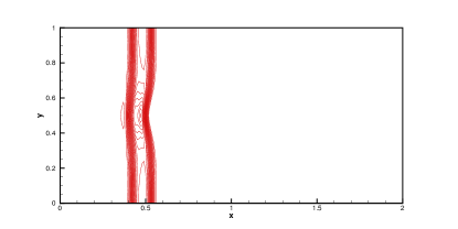
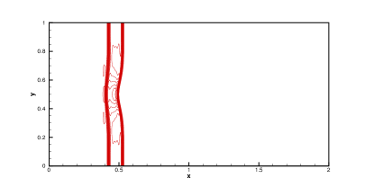
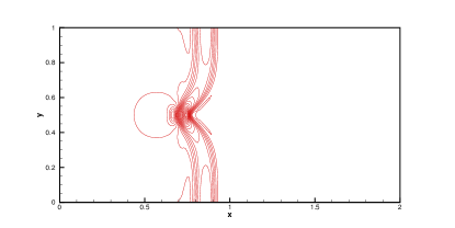
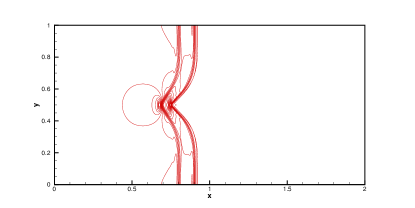
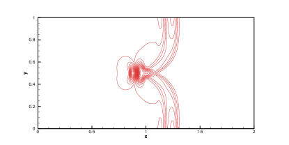
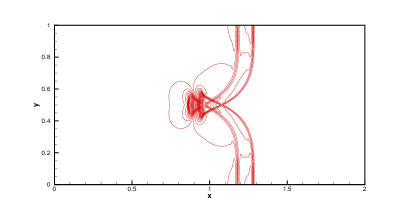
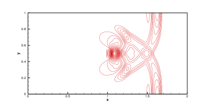
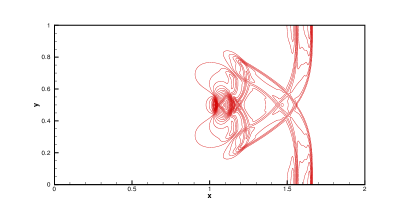
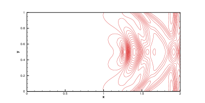
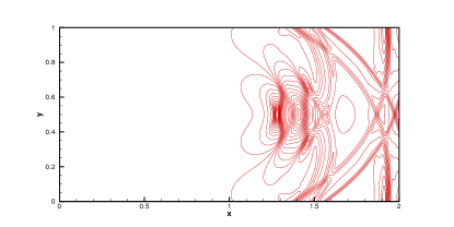
For comparison, we present contours of the water surface level $h+b$ on two different meshes with $200\times 100$ and $600\times 300$ uniform cells in Fig.  10. Fig.  10 displays the right-going disturbance as it propagates past the hump. The numerical results suggest that our schemes can resolve complex small-scale features of the water flow very well. The numerical results are comparable with those in [13].

5 Conclusions

In this paper, we develop a well-balanced finite difference WENO scheme for the shallow water flow model based on equivalent governing equations. Rigorous numerical analysis as well as extensive numerical experiments all suggest that the present scheme maintains the exact C-property for the still water stationary solution. It is also important that the scheme obtains the expected high-order accuracy for smooth solutions, and keeps essentially non-oscillatory property near discontinuities. Based on the current governing equations, the research for the well-balanced finite volume WENO scheme are ongoing.

Appendix A WENO reconstruction procedure for numerical fluxes

By means of the WENO reconstruction procedure, $\hat{f}^{+}_{j+1/2}$ can be expressed as [26]

$$\hat{f}^{+}_{j+1/2}=\sum^{r}_{k=0}\omega_{k}q^{r}_{k}\left(f^{+}_{j+k-r},\ldots,f^{+}_{j+k}\right),$$ (11)

with $\omega_{k}$ being a nonlinear weight, $f^{+}_{i}=f^{+}(u_{i}),\,i=j-r,\ldots,j+r,$ and

$$q^{r}_{k}\left(\mbox{g}_{0},\ldots,\mbox{g}_{r}\right)=\sum^{r}_{l=0}a^{r}_{k,l}\mbox{g}_{l}$$ (12)

are the low order reconstruction to $\hat{f}^{+}_{j+1/2}$ on the $k$th stencil $S_{k}=(x_{j+k-r},\ldots,x_{j+k}),k=0,1,\ldots,r$, and $a^{r}_{k,l},0\leq k,\,l\leq r$ are constant coefficients, see [27] for more details.

The nonlinear weight $\omega_{k}$ in (11) satisfies $\sum\limits^{r}_{k=0}\omega_{k}=1,$ and is designed to yield $(2r+1)$th-order accuracy in smooth regions of the solution. In [26, 27], the nonlinear weight $\omega_{k}$ is formulated as

$$\omega_{k}=\frac{\alpha_{k}}{\sum\limits^{r}_{l=0}\alpha_{l}},\;\mbox{with}\;\alpha_{k}=\frac{C^{r}_{k}}{\left(\varepsilon+IS_{k}\right)^{2}},\,k=0,1,\ldots,r,$$ (13)

where $C^{r}_{k}$ is the linear weight. $IS_{k}$ is a smoothness indicator of $f^{+}(u)$ to measure the smoothness of $f^{+}(u)$ on the stencil $S_{k},\;k=0,1,\ldots,r$, and $\varepsilon$ is a small constant used here to avoid the denominator becoming zero, we take $\varepsilon=10^{-6}$ for all test cases in this paper. We employed the smoothness indicators proposed in [26, 27], i.e.,

$$IS_{k}=\sum^{r}_{l=1}\int^{x_{j+1/2}}_{x_{j-1/2}}(\Delta x)^{2l-1}\left(q_{k}^{(l)}\right)^{2}dx,$$

where $q^{(l)}_{k}$ is the $l$th-derivative of $q_{k}(x)$ and $q_{k}(x)$ is the reconstruction polynomial of $f^{+}(u)$ on stencil $S_{k}$ such that

$$\frac{1}{\Delta x}\int_{I_{i}}q_{k}(x)dx=f^{+}_{i},\,i=j+k-r,\ldots,j+k.$$

The procedure for the reconstruction of $\hat{f}^{-}_{j+\frac{1}{2}}$ is a mirror symmetry to that of $\hat{f}^{+}_{j+1/2}$ with respect to the grid point $x_{j+1/2}$, so we will not present it here to save space.

Appendix B Verification of the linearity of the scheme

By virtue of the WENO reconstruction procedure, $\hat{f}^{+}_{j+1/2}$ can be written out in the following form

$$\begin{array}[]{lcl}\hat{f}^{+}_{j+1/2}&=&\sum\limits_{k=-r}^{r}c_{k}f^{+}_{j+k}\\ &=&\sum\limits_{k=-r}^{r}c_{k}\left[\frac{1}{2}\left(f_{j+k}+\alpha U_{j+k}\right)\right]\\ &=&\frac{1}{2}\sum\limits_{k=-r}^{r}c_{k}f_{j+k}+\frac{1}{2}\sum\limits_{k=-r}^{r}c_{k}\left(\alpha U_{j+k}\right),\end{array}$$ (14)

where $f^{+}=f^{+}(U)$ as in (8), $c_{k}$ is a $2\times 2$ matrix depending nonlinearly on the smoothness indicators of $f^{+}$ on the stencil $\{x_{j-r},\ldots,x_{j+r}\}$, and $\alpha$ is a $2\times 2$ diagonal matrix involving $\alpha_{i}$ in (9).

Analogously, we can write $\hat{f}^{-}_{j+1/2}$ as follows

$$\begin{array}[]{lcl}\hat{f}^{-}_{j+1/2}&=&\sum\limits_{k=-r+1}^{r+1}a_{k}f^{-}_{j+k}\\ &=&\sum\limits_{k=-r+1}^{r+1}a_{k}\left[\frac{1}{2}\left(f_{j+k}-\alpha U_{j+k}\right)\right]\\ &=&\frac{1}{2}\sum\limits_{k=-r+1}^{r+1}a_{k}f_{j+k}-\frac{1}{2}\sum\limits_{k=-r+1}^{r+1}a_{k}\left(\alpha U_{j+k}\right),\end{array}$$ (15)

where $a_{k}$ is also a $2\times 2$ matrix depending nonlinearly on the smoothness indicators of $f^{-}$ on the stencil $\{x_{j-r+1},\ldots,x_{j+r+1}\}$.

So we have

$$\hat{f}_{j+1/2}=\hat{f}_{j+1/2}^{+}+\hat{f}_{j+1/2}^{-}.$$ (16)

Similarly, $\hat{f}_{j-1/2}^{+}$ has the following form

$$\begin{array}[]{lcl}\hat{f}_{j-1/2}^{+}&=&\sum\limits_{k=-r-1}^{r-1}\hat{c}_{k}f_{j+k}^{+}\\ &=&\sum\limits_{k=-r-1}^{r-1}\hat{c}_{k}\left[\frac{1}{2}\left(f_{j+k}+\alpha U_{j+k}\right)\right]\\ &=&\frac{1}{2}\sum\limits_{k=-r-1}^{r-1}\hat{c}_{k}f_{j+k}+\frac{1}{2}\sum\limits_{k=-r-1}^{r-1}\hat{c}_{k}\left(\alpha U_{j+k}\right),\end{array}$$ (17)

where $\hat{c}_{k}$ is a $2\times 2$ matrix depending nonlinearly on the smoothness indicators of $f^{+}$ on the stencil $\{x_{j-r-1},\ldots,x_{j+r-1}\}$.

Finally, $\hat{f}_{j-1/2}^{-}$ can be written out in the below form

$$\begin{array}[]{lcl}\hat{f}_{j-1/2}^{-}&=&\sum\limits_{k=-r}^{r}c_{k}f_{j-k}^{-}\\ &=&\sum\limits_{k=-r}^{r}c_{k}\left[\frac{1}{2}\left(f_{j-k}-\alpha U_{j-k}\right)\right]\\ &=&\frac{1}{2}\sum\limits_{k=-r}^{r}c_{k}f_{j-k}-\frac{1}{2}\sum\limits_{k=-r}^{r}c_{k}\left(\alpha U_{j-k}\right),\end{array}$$ (18)

where $c_{k}$ is the same $2\times 2$ matrix as in (14).

Consequently, we can obtain

$$\hat{f}_{j-1/2}=\hat{f}_{j-1/2}^{+}+\hat{f}_{j-1/2}^{-}.$$ (19)

With the formulae in (14), (15), (17) and (18), the approximation to $f(U)_{x}$ can be eventually written out as follows

$$\begin{array}[]{lcl}f\left(U\right)_{x}|_{x=x_{j}}&\approx&\frac{1}{\Delta x}\left(\hat{f}_{j+1/2}-\hat{f}_{j-1/2}\right)\\ &=&\frac{1}{\Delta x}\left[\left(\frac{1}{2}\sum\limits_{k=-r}^{r}c_{k}f_{j+k}+\frac{1}{2}\sum\limits_{k=-r}^{r}c_{k}(\alpha U_{j+k})+\frac{1}{2}\sum\limits_{k=-r+1}^{r+1}a_{k}f_{j+k}-\frac{1}{2}\sum\limits_{k=-r+1}^{r+1}a_{k}\left(\alpha U_{j+k}\right)\right)\right.\\ &-&\left.\left(\frac{1}{2}\sum\limits_{k=-r-1}^{r-1}\hat{c}_{k}f_{j+k}+\frac{1}{2}\sum\limits_{k=-r-1}^{r-1}\hat{c}_{k}(\alpha U_{j+k})+\frac{1}{2}\sum\limits_{k=-r}^{r}c_{k}f_{j-k}-\frac{1}{2}\sum\limits_{k=-r}^{r}c_{k}\left(\alpha U_{j-k}\right)\right)\right]\\ &=&\frac{1}{2\Delta x}\left(\sum\limits_{k=-r}^{r}c_{k}f_{j+k}-\sum\limits_{k=-r-1}^{r-1}\hat{c}_{k}f_{j+k}\right)\\ &+&\frac{1}{2\Delta x}\left(\sum\limits_{k=-r+1}^{r+1}a_{k}f_{j+k}-\sum\limits_{k=-r}^{r}c_{k}f_{j-k}\right)\\ &+&\frac{1}{2\Delta x}\left(\sum\limits_{k=-r}^{r}c_{k}(\alpha U_{j+k})-\sum\limits_{k=-r-1}^{r-1}\hat{c}_{k}(\alpha U_{j+k})\right)\\ &+&\frac{1}{2\Delta x}\left(\sum\limits_{k=-r}^{r}c_{k}(\alpha U_{j-k})-\sum\limits_{k=-r+1}^{r+1}a_{k}\left(\alpha U_{j+k}\right)\right)\\ &=&\mathbf{P1}+\mathbf{P2}+\mathbf{P3}+\mathbf{P4}.\end{array}$$ (20)

Subsequently, we will verify that the formula $\frac{1}{\Delta x}\left(\hat{f}_{j+1/2}-\hat{f}_{j-1/2}\right)$ for the approximation to $f\left(U\right)_{x}|_{x=x_{j}}$ is a finite difference operator. It should be noted that with $\pm\alpha U=\pm\alpha\left(\begin{array}[]{c}H\\ hu\end{array}\right)$ in the flux splitting (8), this vector becomes a constant vector for the still water stationary solution (2). By $U$ we denote $U_{j+k}$ with an abuse of notation. So $\alpha U_{j+k}=\alpha U$ is also a constant vector. Thus

$$\begin{array}[]{lcl}\mathbf{P3}&=&\frac{1}{2\Delta x}\left(\sum\limits_{k=-r}^{r}c_{k}(\alpha U_{j+k})-\sum\limits_{k=-r-1}^{r-1}\hat{c}_{k}(\alpha U_{j+k})\right)\\ &=&\frac{1}{2\Delta x}\left(\sum\limits_{k=-r}^{r}c_{k}(\alpha U)-\sum\limits_{k=-r-1}^{r-1}\hat{c}_{k}(\alpha U)\right)\\ &=&\frac{1}{2\Delta x}\left[\left(\sum\limits_{k=-r}^{r}c_{k}\right)(\alpha U)-\left(\sum\limits_{k=-r-1}^{r-1}\hat{c}_{k}\right)(\alpha U)\right]\\ &=&\frac{1}{2\Delta x}\left[I\cdot(\alpha U)-I\cdot(\alpha U)\right]\\ &=&0,\end{array}$$ (21)

where $I$ is a $2\times 2$ identity matrix, the equivalents $\sum\limits_{k=-r}^{r}c_{k}=I$ and $\sum\limits_{k=-r-1}^{r-1}\hat{c}_{k}=I$ are due to the consistency of the WENO reconstruction.

For the still water stationary solution (2), and with the similar procedure as above, we can obtain that

$$\mathbf{P4}=\frac{1}{2\Delta x}\left(\sum\limits_{k=-r}^{r}c_{k}(\alpha U_{j-k})-\sum\limits_{k=-r+1}^{r+1}a_{k}(\alpha U_{j+k})\right)=0.$$ (22)

As a result, the approximation to $f(U)_{x}$ in (20) can be eventually written out as

$$\begin{array}[]{rcl}f(U)_{x}|_{x=x_{j}}&\approx&\frac{1}{\Delta x}(\hat{f}_{j+1/2}-\hat{f}_{j-1/2})\\ &=&\mathbf{P1}+\mathbf{P2}\\ &=&\frac{1}{2\Delta x}\left(\sum\limits_{k=-r}^{r}c_{k}f_{j+k}-\sum\limits_{k=-r-1}^{r-1}\hat{c}_{k}f_{j+k}\right)+\frac{1}{2\Delta x}\left(\sum\limits_{k=-r+1}^{r+1}a_{k}f_{j+k}-\sum\limits_{k=-r}^{r}c_{k}f_{j-k}\right)\\ &=&\sum\limits_{k=-r-1}^{r+1}\beta_{k}f_{j+k}\\ &\triangleq&D_{f}(f)\big{|}_{x=x_{j}},\end{array}$$ (23)

where $D_{f}$ denotes a finite difference operator depending the flux $f(U)$ and $\beta_{k}$ is a $2\times 2$ matrx depending on the smoothness indicators involving $f^{+}(U)$ and $f^{-}(U)$. The key idea of our scheme is to apply the operator $D_{f}$ in (23) with the fixed coefficient matrix $\beta_{k}$, to approximate the source term $(0,b)_{x}^{T}$. This amounts to split the source term as

$$\left(\begin{array}[]{c}0\\ b\end{array}\right)_{x}=\frac{1}{2}\left(\begin{array}[]{c}0\\ b\end{array}\right)_{x}+\frac{1}{2}\left(\begin{array}[]{c}0\\ b\end{array}\right)_{x},$$ (24)

and apply the finite difference operator $D_{f}$ to approximate them. Concretely speaking, one half part of the source term is approximated by the operator $D_{f}$ with coefficients obtained from the computation of $f^{+}(U)$, and the remaining part by the operator $D_{f}$ with coefficients coming from the computation of $f^{-}(U)$.

A key observation is that the operator $D_{f}$ in (23) with the fixed coefficient matrices $\beta_{k}$ is a linear finite difference operator on any grid function as in (7). We thus conclude that for the still water stationary solution (2), the present WENO scheme is a linear scheme, even with the global Lax-Friedrichs flux splitting (8) as well as the local characteristic decomposition procedure.

Table 1: $L^{1}$ errors and orders of accuracy for the test case in Section 4.1.2.

	$h$		$hu$
N	$L^{1}\;\mbox{error}$	Order	$L^{1}\;\mbox{error}$	Order
25	1.7486E-02		1.1294E-01
50	2.2133E-03	2.98	1.9663E-02	2.52
100	3.3157E-04	2.74	2.8131E-03	2.81
200	2.3391E-05	3.83	2.0167E-04	3.80
400	9.4357E-07	4.63	8.1928E-06	4.62
800	2.9898E-08	4.98	2.5426E-07	5.01

Table 2: $L^{1}$ and $L^{\infty}$ error for different precisions for the still water stationary solution over a smooth bottom topography.

	$L^{1}\,\,\mbox{error}$		$L^{\infty}\,\,\mbox{error}$
Precision	$h$	$hu$	$h$	$hu$
Single	1.14E-06	1.612E-06	3.81E-06	5.23E-06
Double	6.14E-16	4.12E-15	1.95E-15	1.48E-16
Quadruple	1.57E-33	2.94E-32	6.98E-33	9.12E-32

Table 3: $L^{1}$ and $L^{\infty}$ error for different precisions for the still water stationary solutions over a discontinuous bottom topography.

	$L^{1}\,\,\mbox{error}$		$L^{\infty}\,\,\mbox{error}$
Precision	$h$	$hu$	$h$	$hu$
Single	1.53E-06	3.70E-07	1.91E-06	2.53E-06
Double	4.35E-16	3.62E-15	1.60E-16	1.17E-15
Quadruple	1.43E-33	2.15E-32	4.09E-33	5.64E-32

Table 4: $L^{1}$ for different precisions for the still water stationary solutions over a non-flat bottom topography.

	$L^{1}\,\,\mbox{error}$
Precision	$h$	$hu$	$hv$
Single	5.83E-08	2.91E-07	2.93E-07
Double	1.63E-16	6.43E-16	6.45E-16
Quadruple	2.13E-34	4.65E-34	4.39E-34

Table 5: $L^{1}$ errors and orders of accuracy for the test case in Section 4.2.2.

	$h$		$hu$		$hv$
$N_{x}\times N_{y}$	CFL	$L^{1}\;\mbox{error}$	Order	$L^{1}\;\mbox{error}$	Order	$L^{1}\;\mbox{error}$	Order
$25\times 25$	0.6	1.1878E-002		3.6702E-002		9.8931E-002
$50\times 50$	0.6	1.4841E-003	3.00	4.5263E-003	3.02	1.3532E-002	2.87
$100\times 100$	0.6	1.1262E-004	3.72	3.5071E-004	3.69	1.0558E-003	3.68
$200\times 200$	0.4	4.9428E-006	4.51	1.6844E-005	4.38	4.6660E-005	4.50
$400\times 400$	0.3	1.7866E-007	4.79	6.6166E-007	4.67	1.6866E-006	4.79
$800\times 800$	0.2	6.0255E-009	4.89	2.3751E-008	4.80	5.6882E-008	4.89

Fig. 1: Small perturbation of a steady state water flow with a big pulse, $t=0.2$ s. Water surface level $h+b$ (left) and water discharge $hu$ (right).

Fig. 2: Small perturbation of a steady state water flow with a small pulse, $t=0.2$ s. Water surface level $h+b$ (left) and water discharge $hu$ (right).

Fig. 3: Transcritical flow without a shock, $t=200$ s. Water surface level $h+b$ (left) and water discharge $hu$ (right).

Fig. 4: Transcritical flow with a shock, $t=200$ s. Water surface level $h+b$ (left) and water discharge $hu$ (right).

Fig. 5: Subcritical flow, $t=200$ s. Water surface level $h+b$ (left) and water discharge $hu$ (right).

Fig. 6: The dam break problem over a rectangular bump. Water surface level $h+b$ at $t=15$ s (left) and $t=60$ s (right).

Fig. 7: The tidal wave flow, $t=7552.13$ s. Water depth $h$ (left) and water velocity $u$ (right).

Fig. 8: $1$-rarefaction and $2$-shock problem, $t=1$ s. Water surface level $h+b$ (left) and water discharge $hu$ (right).

Fig. 9: 1-shock and 2-shock problem, $t=1$ s. Water surface level $h+b$ (left) and water discharge $hu$ (right).

Fig. 10: A small perturbation of a two-dimensional steady state water flow. Contours of water surface level h+b at different end time. From top to bottom: at time $t=0.12$ s from $0.999703$ to $1.00629$; at time $t=0.24$ s from $0.994836$ to $1.01604$; at time $t=0.36$ s from $0.988582$ to $1.0117$; at time $t=0.48$ s from $0.990344$ to $1.00497$; and at time $t=0.6$ s from $0.995065$ to $1.0056$. Left: numerical results on a mesh with $200\times 100$ uniform cells. Right: numerical results on a mesh with $600\times 300$ uniform cells.

References

- [1] S.F. Bradford, B.F. Sanders, Finite volume model for shallow water flooding of arbitrary topography, J. Hydraul. Eng-ASCE. 128 (2002) 289-298.
- [2] G. Gottardi, M. Venutelli, Central scheme for the two-dimensional dam-break flow simulation, Adv. Water. Resour. 27 (2004) 259-268.
- [3] M.E. Vazquez-Cendon, Improved treatment of source terms in upwind schemes for the shallow water equations in channels with irregular geometry, J. Comput. Phys. 148(1999) 497-526.
- [4] S. Jin, A steady state capturing method for hyperbolic systems with geometrical source terms, Math. Model. Num. Ana. 35 (2001) 631-646.
- [5] A. Kurganov, D. Levy, Central-upwind schemes for the Saint-Venant system, Math. Model. Num. Ana. 36 (2002) 397-425.
- [6] A. Bermudez, M.E. Vazquez, Upwind methods for hyperbolic conservation laws with source terms, Comput. Fluids. 23 (1994) 1049-1071.
- [7] J.M. Greenberg, A.Y. Leroux, A well-balanced scheme for the numerical processing of source terms in hyperbolic equations, SIAM J. Numer. Anal. 33 (1996) 1-16.
- [8] J.M. Greenberg, A.Y. Leroux, R. Baraille, A. Noussair, Analysis and approximation of conservation laws with source terms, SIAM J. Numer. Anal. 34 (1997) 1980-2007.
- [9] S. Noelle, Y.L. Xing, C.-W. Shu, High-Order Well-balanced Schemes. in: Numerical Methods for Balance Laws (G. Puppo and G. Russo eds). Quaderni di Matematica (2010).
- [10] Y.L. Xing, C.-W. Shu, S. Noelle, On the advantage of well-balanced schemes for moving-water equilibria of the shallow water equations, J. Sci. Comput. 48 (2011) 339-349.
- [11] R.J. LeVeque, Balancing source terms and flux gradient on high-resolution Godunov methods: the quasi-steady wave-propagation algorithm, J. Comput. Phys. 146 (1998) 346-365.
- [12] J.G. Zhou, D.M. Causon, C.G. Mingham, D.M. Ingram, The surface gradient method for the treatment of source terms in the shallow-water equations, J. Comput. Phys. 168 (2001) 1-25.
- [13] Y.L. Xing, C.-W. Shu, High order finite difference WENO schemes with the exact conservation property for the shallow water equations, J. Comput. Phys. 208 (2005) 206-227.
- [14] Y.L. Xing, C.-W. Shu, High-order well-balanced finite difference WENO schemes for a class of hyperbolic systems with source terms, J. Sci. Comput. 27 (2006) 477-494.
- [15] Y.L. Xing, C.-W. Shu, High order well-balanced finite volume WENO schemes and discontinuous Galerkin methods for a class of hyperbolic systems with source terms, J. Comput. Phys. 214 (2006) 567-598.
- [16] Y.L. Xing, C.-W. Shu, A new approach of high order well-balanced finite volume WENO schemes and discontinuous Galerkin methods for a class of hyperbolic systems with source terms, Commun. Comput. Phy. 1 (2006) 100-134.
- [17] E. Audusse, F. Bouchut, M.O. Bristeau, R. Klein, B. Perthame, A fast and stable well-balanced scheme with hydrostatic reconstruction for shallow water flows, SIAM J. Sci. Comput. 25 (2004) 2050-2065.
- [18] E. Audusse, M.O. Bristeau, A well-balanced positivity preserving “second-order” scheme for shallow water flows on unstructured meshes, J. Comput. Phys. 206 (2005) 311-333.
- [19] S. Noelle, N. Pankratz, G. Puppo, J.R. Natvig, Well-balanced finite volume schemes of arbitrary order of accuracy for shallow water flows, J. Comput. Phys. 213 (2006) 474-499.
- [20] V. Caleffi, A new well-balanced Hermite weighted essentially non-oscillatory scheme for shallow water equations, Int. J. Numer. Meth. Fl. 67 (2011) 1135-1159.
- [21] J.X. Qiu, C.-W. Shu, Hermite WENO schemes and their application as limiters for Runge-Kutta discontinuous Galerkin method: one-dimensional case, J. Comput. Phys. 193 (2003) 115-135.
- [22] J.M. Hou, F. Simons, M. Mahgoub, R. Hinkelmann, A robust well-balanced model on unstructured grids for shallow water flows with wetting and drying over complex topography, Comput. Methods. Appl. Mech. Eng. 257 (2013) 126-149.
- [23] B.D. Rogers, A. Borthwick, and P.Taylor. Mathematical balancing of flux gradient and source terms prior to using Roes approximate Riemann solver. J. Comput. Phys. 192 (2003) 422-451.
- [24] A. Canestrelli, A. Siviglia, M. Dumbser, E.F. Toro, Well-balanced high-order centred schemes for non-conservative hyperbolic systems. Applications to shallow water equations with fixed and mobile bed, Adv. Water. Resour. 32 (2009) 834-844.
- [25] G. Li, V. Caleffi, J.M. Gao, High-order well-balanced central WENO scheme for pre-balanced shallow water equations, Comput. Fluids. 99 (2014) 182-189.
- [26] G.S. Jiang, C.-W. Shu, Efficient implementation of weighted ENO Schemes, J. Comput. Phys. 126 (1996) 202-228.
- [27] C.-W. Shu, Essentially non-oscillatory and weighted essentially non-oscillatory schemes for hyperbolic conservation laws, NASA/CR-97-206253, ICASE Report NO.97-65.
- [28] C.-W. Shu, High order weighted essentially nonoscillatory schemes for convection dominated problem, SIAM Rev. 51 (2009) 82-126.
- [29] C.-W. Shu, S. Osher, Efficient implementation of essentially non-oscillatory shock-capturing schemes, J. Comput. Phys. 77 (1988) 439-471.
- [30] G. Kesserwani, Q.H. Liang, A discontinuous Galerkin algorithm for the two-dimensional shallow water equations, Comput. Methods. Appl. Mech. Eng. 199 (2010) 3356-3368.
- [31] N. Goutal, F. Maurel, Proceedings of the Second Workshop on Dam-Break Wave Simulation, Technical Report HE-43/97/016/A, Electricit de France, Dpartement Laboratoire National d’Hydraulique, Groupe Hydraulique Fluviale, 1997.
- [32] S. Vukovic, L. Sopta, ENO and WENO schemes with the exact conservation property for one-dimensional shallow water equations, J. Comput. Phys. 179 (2002) 593-621.
- [33] A. Bermudez, M.E. Vazquez, Upwind methods for hyperbolic conservation laws with source terms, Comput. Fluids. 23 (1994) 1049-1071.
- [34] F. Alcrudo, F. Benkhaldoun, Exact solution to the Riemann problem of the shallow water euqaionts with a bottom step, Comput. Fluids. 30 (2001) 643-671.
- [35] F. Benkhaldoun, I. Elmahi, M. Seaid M. Well-balanced finite volume schemes for pollutant transport by shallow water equations on unstructured meshes, J. Comput. Phys. 226 (2007) 180-203.