A Bayesian Approach to Rule Mining
Abstract
In this paper, we introduce the increasing belief criterion in association rule mining. The criterion uses a recursive application of Bayes’ theorem to compute a rule’s belief. Extracted rules are required to have their belief increase with their last observation. We extend the taxonomy of association rule mining algorithms with a new branch for Bayesian rule mining (BRM), which uses increasing belief as the rule selection criterion. In contrast, the well-established frequent association rule mining (FRM) branch relies on the minimum-support concept to extract rules.
We derive properties of the increasing belief criterion, such as the increasing belief boundary, no-prior-worries, and conjunctive premises. Subsequently, we implement a BRM algorithm using the increasing belief criterion, and illustrate its functionality in three experiments: (1) a proof-of-concept to illustrate BRM properties, (2) an analysis relating socioeconomic information and chemical exposure data, and (3) mining behaviour routines in patients undergoing neurological rehabilitation. We illustrate how BRM is capable of extracting rare rules and does not suffer from support dilution. Furthermore, we show that BRM focuses on the individual event generating processes, while FRM focuses on their commonalities. We consider BRM’s increasing belief as an alternative criterion to thresholds on rule support, as often applied in FRM, to determine rule usefulness.
Index Terms:
Association Rule mining, Bayesian Rule Mining, Increasing belief criterion, Increasing belief boundary.1 Introduction
Association rules can model a process by describing the relationship between its variables. In a dynamic process, for example, a rule states that a change on an input will cause a change on an output. As the process’ evolution is stored in a dataset, rule mining can extract the original relationship between the process’ inputs and outputs. The frequently applied paradigm for mining rules is frequent association rule mining (FRM). Rules extracted by FRM, e.g., , have their support greater than a set threshold called minimum-support. The literature defines support as in Equation 1, where is the rule’s occurrence count and is the dataset size [1].
| (1) |
The following thought experiment illustrates one of FRM’s limitations. Suppose we use all supermarket receipts from the winter holidays for rule mining. Then, we would see rules that associate the ingredients used for winter holiday meals. However, if we now consider a year worth of receipts from the same supermarket, then, the winter holiday meal ingredients would not have enough support to be extracted. In other words, the minimum-support threshold used to extract rules in a small dataset will not work in an extended version of the dataset due to the definition of rule support. We refer to FRM’s dependency on the dataset size as support dilution.
Another FRM limitation appears when a dataset contains multiple processes. FRM has the implicit assumption that all processes generate symbols at the same rate. However, in practice, processes can generate symbols at different rates. For example, people in Germany occasionally buy white sausages, but when they do, they always buy wheat beer. So the rule ‘if white sausage then wheat beer’ is a rare rule when compared to frequent rules, e.g., ‘if milk then eggs’. FRM can extract rare rules by using a low minimum-support threshold. Unfortunately, spurious symbol associations may create unwanted rules that FRM’s threshold cannot eliminate. Filtering out unwanted rules for FRM has been addressed in the past [2, 3]. However, we observed that the processing required to separate rules does not generalise.
To bypass FRM’s support dilution and rare rule extraction limitations, we propose to exploit the belief concept of Bayesian filtering and derive an increasing belief criterion. We drew inspiration from Price’s account of Bayes views on updating beliefs [4]. Price illustrates the idea with an example of a group of cavemen coming out into the world for the first time. The first thing the cavemen will probably notice is the sun, and how the sun moves through the sky until it disappears. At this point, the cavemen are unaware if the sun will appear again. As the sun rose and set during the next days, the cavemen will update their belief about the sun setting and rising as a defining feature of the way the world works outside the cave.
In this work, we present the following contributions:
(1) We extend the taxonomy
of association rule mining by a branch for Bayesian rule mining (BRM), which
uses increasing belief as rule mining criterion.
(2) We introduce the increasing belief criterion, derive key properties, and show their
application.
(3) We implement an exhaustive search BRM
algorithm and demonstrate its viability as solution for support dilution and
rare rule extraction, by extracting rules in three datasets: a synthetic time
series, a dataset linking socio-economic variables with chemical-exposure
information, and a dataset of daily behaviour routine annotations of patients
with hemiparesis. In each experiment, we compared rules extracted by BRM and FRM
and evaluated their quality and usefulness for each application.

2 Related Work
Association rule mining algorithms can be organised into branches by their main rule selection criteria. We consider two algorithm branches: the FRM branch, which uses support to extract rules, and the BRM branch, which uses increasing belief. Figure 1 illustrates the first four levels of our proposed taxonomy. The use of minimum-support determines the first subclasses level for FRM, and the method used for finding frequent symbol sets defines the next level. Padillo et al. [6] provided a comprehensive list of the FRM algorithms, and we expanded on the FRM taxonomy of optimisation algorithms that use minimum-support proposed by Beiranvand et al. [5]. To our knowledge, and except for our initial work on BRM [7], the entirety of research on association rule mining belongs to the FRM branch. In the BRM branch, the method used to find relevant symbol sets determines the first subclass level. We have added the optimisation block as a place holder for future research.
Below, we elaborate on the FRM methods along the taxonomy. The related work is organized in three subsections. First, we follow the taxonomy illustrated in Fig. 1 to present FRM methods. Next, we provide examples of work that considered the challenge of rare rule extraction. Finally, we describe our previous work in BRM.
2.1 Frequent Association Rule Mining Branch
2.1.1 Minimum-support, Exhaustive
An exhaustive search algorithm has to traverse the lattice created from the symbol’s power set. The downward-closure property [8] can be used to facilitate lattice traversal. The property states that the support of any symbol set is less or equal to the support of any of its possible subsets. Therefore, exhaustive search algorithms can ignore entire branches of the symbol set lattice when a given set does not pass the minimum-support threshold.
The use of the downward-closure property divides FRM’s exhaustive search class into two subclasses. OPUS is an example of exhaustive search algorithms that do not use the downward-closure property to traverse the symbol lattice. Webb [9] created OPUS as a frequent-set mining algorithm. Subsequently, Webb [10] presented an extension that converted OPUS into a rule mining algorithm. The Apriori [11] and ECLAT [12] algorithms use the downward-closure property and define two distinct approaches on how to traverse the symbol set lattice. The Apriori algorithm uses a breadth-first approach. The algorithm starts with all one symbol sets and traverses the lattice upwards using the downward-closure property. The ECLAT algorithm uses a depth-first approach, starting with one symbol and traversing the lattice in depth using the downward-closure property to avoid infrequent branches. Exhaustive search algorithms in BRM can use the premise-conjunction property (Property 3) to simplify the search for premise symbol sets with more than one element. Our proposed algorithm uses a breadth-first approach to traverse the symbol lattice.
2.1.2 Minimum-support, Optimisation
Evolutionary algorithms use genetic optimization or swarms to find the most common symbol sets. The general approach is to write maximization objectives which are usually functions of support and confidence [13, 14, 15]. However, most approaches still need a minimum-support threshold to select rules. BRM opens a new area of research, as the increasing belief criterion can be integrated with evolutionary algorithms, thus replacing support and related measures of rule interest.
Rule grammars and machine learning approaches have been presented as alternatives of the downward-closure property to restrict rule search space. For example, Padillo et al. [6] uses rule grammar and map reduce to optimize the mining process in large datasets. Rule grammars can be used seamlessly with increasing belief, and rule belief can be maximized using map reduce by means of Prop. 1. In timeseries, Guillam-Bert et al. [16] proposed the TITARl algorithm. They used decision trees to improve rule description and specificity, specially when regarding time.
2.1.3 Other FRM Algorithms
Other algorithms in FRM do not use minimum-support as part of the rule selection process. ARMGA and EARMGA are optimisation algorithms proposed by Yan et al. [17]. (E)ARMGA uses a genetic programming approach with relative confidence as the fitness function. The algorithm searches for the best rules until it reaches a maximum number of generations or the difference between the relative confidence of the best and worst individuals is less than a parameter . By avoiding the minimum-support threshold, (E)ARMGA does not suffer from support dilution. However, as data is added that does not maintain the distribution of initial rule’s symbols, relative confidence increases and tends to one, regardless of the relative frequencies of the premise and conclusion sets. Furthermore, the parameter is difficult to set without solving the rule mining problem, i.e., without doing a parametric search.
Bashir et al. [13] proposed an exhaustive search algorithm, which starts by selecting symbol sets. Then, their algorithm selects the smallest support values of the chosen symbols sets, and prunes the search space using the downward-closure property. The search process is repeated looking for sets with higher support. As there are always selected sets, the value for pruning the search spaced is set to the smallest support value.
2.2 Rare Rule Extraction
When researchers applied rule mining to practical problems, they noted that the most-frequent rules were not always the most interesting. For example, in activities of daily living, some patterns, like walking and talking, occur frequently, but do not yield interesting rules. Therefore, several rule interest metrics were proposed, including lift [18], conviction [19], among others, to prune the final rule set. Nevertheless, rule interest metrics are either based on support or depend on frameworks that use minimum-support to select the initial candidate rule set. We argue that the use of support to preselect rules causes the mining algorithm to miss rare but essential rules. For example, consider a ceiling lamp controlled by motion and the absence of daylight. While motion may often trigger the lamp, in comparison, absence of daylight will only trigger the lamp a couple of times a day. As a result, finding the relation between the absence of daylight and the lamp being triggered is difficult based on support alone [2].
The common tactic to solve rare rule problems is to use a sufficiently low minimum-support threshold. Then, algorithms use rule interest metrics to extract interesting and rare rules. For example, Liu et al. [20] proposed a methodology to extract intricate activity patterns from timeseries. Their method searches for rules in a region bounded by minimum-support and confidence thresholds. The final rules are selected using a threshold on information gain. A similar approach was implemented by Liu et al. [3]. They proposed a support band to determine a rule’s rarity. In contrast, Srinivasan et al.[21] proposed a method for extracting conditional action rules using four new rule selection criteria. However, their framework uses a minimum-support threshold to mine frequent symbol sets.
2.3 Bayesian Rule Mining Branch
We expand on our initial BRM work [7] by refining the theoretical derivation and mined rule handling. Moreover, we introduced two additional properties of increasing belief, add an optional control parameter, extend the algorithm for database mining, and present three new evaluation scenarios.
3 Increasing Belief Criterion
We defined belief in a rule as the recursive application of the Bayes theorem, as shown in Definition 1. The initial belief of a rule is the probability of observing the conclusion given that the premise was observed, i.e., . Using the Bayes theorem, is calculated using the probability and the prior . In general, can be estimated by the ratio , where is the th observation of the rule and is the number of times is observed at the th observation of . Thus, in the initial state, . The prior is an algorithm parameter. and denote the compliments of and , respectively. Finally, in the recursive evaluation of , the previous belief evaluation (), replaces the prior . A common criticism of Bayesian methods is the challenge of selecting the correct prior probabilities. However, as explained in Prop. 4, a prior in range has no effect on the rule selection process.
Definition 1 (Belief).
Recursive definition of belief.
The increasing belief criterion requires that a rule’s belief does not decrease with respect to the previous observation, as shown in Def. 2.
Definition 2 (Increasing Belief Criterion).
A rule has increasing belief, at observation , when .
3.1 Properties and Proofs
Here, we present the properties we derived from the rule selection criterion of increasing belief (Def. 2).
Property 1 (Increasing Belief Boundary).
The belief of a rule will increase or stay constant if the conditional probability is equal or greater than 0.5.
Proof.
Property 2 (Saturation).
If a rule reaches belief of one, new independent symbol observations will not alter the rule’s belief.
Proof.
Assume the belief is one.
| Def. 1 | |||||
| Using the assumption | |||||
In saturation, changes to the probability , i.e., the ratio between rule observations and the conclusion symbol observations, have no effect on the rule’s belief. ∎
Corollary 2.1.
Rules created with the first observation of a symbol as conclusion have saturated belief.
Proof.
Note that when the rule and its conclusion symbol are observed for the first time, the probability
Replacing the value of in Def. 1 for yields . Therefore, the rule is in saturation. ∎
Corollary 2.2.
A similar saturation effect occurs when the rule’s belief is equal to zero.
Proof.
When , then, by Def. 1, , regardless of the value of . ∎
Property 3 (Premise Conjunction).
If a rule with a conjunction of symbols as premise has increasing belief, its atomic rule constituents also have increasing belief.
Proof.
Suppose that rule is of the form and it has increasing belief, but the constituent atomic rule of the form has not. Let , , , and denote the number of times the rule and its atomic constituents were observed in the dataset. Additionally, is the number of times was observed in the dataset.
| Assumption and | |||||
| Prop. 1 | |||||
Contradiction. cannot be and simultaneously. ∎
Corollary 3.1.
A similar argument to conjunctive premises cannot be made for rule conclusions. The atomic constituents of a conjunctive conclusion rule are not required to have increasing belief for to pass the increasing belief criterion. The constituent atomic rule frequencies have no effect on the rules’ belief.
Proof.
Assume there is a rule , where is a combination of symbols occurring only once in the dataset. Therefore, the rule occurs only once too. Furthermore, implying that the rule has increasing belief due to Prop. 1. As a result, the constituent atomic rule’s belief has no relevance for the rule with a conjunctive conclusion. ∎
Property 4 (No-Prior-Worries).
For the increasing belief criterion, the prior parameter has no effect for rule selection and any value in the open interval can be used. Using zero or one as will cause the rule’s belief to saturate (Prop. 2).
Proof.
We look at the first iteration of the belief evaluation criteria.
| By Defs. 1 and 2 | |||
| Avoid saturation – Prop. 2 | |||
∎
Remark.
Although the prior has no effect on rule selection, the prior determines a rule’s final belief value.
4 Implementation of the BRM algorithm
Algorithm 1 describes BRM’s procedure, where is a dataset, and is a respective record or observation window in . Observation windows are used to analyse timeseries. The algorithm parameter sets the size of the observation window. During analysis, the observation window moves in steps of one symbol. With properly defined, BRM creates candidate rules from each using select_candidate_rules. Candidate rules are created in two different ways depending on whether is a database or a timeseries. For a timeseries, and to respect time dependency, the candidate rules are the result of pairing the first symbol in the observation window with all remaining symbols. In contrast, for a database, the candidate rules are all pairwise combinations of symbols in the record. Next, pass_selection_criteria(CR) returns a set of candidate rules that pass the selection criterion shown in Def. 2. The rules returned by pass_selection_criteria(CR) are added to the rule set . Subsequently, any rule in that fails the selection criterion is removed from . BRM only requires one pass of .
BRM only evaluates a rule’s increasing belief criterion when the rule is observed. Therefore, once BRM processed the entire dataset, rules are checked for loss of belief and removed if necessary. Loss of belief can occur in two cases: (1) the rule’s belief saturated (Prop. 2) and additional observations did not change the rule’s belief, or, (2) at the end of the dataset, BRM observed extra conclusion symbols without corresponding rule observations. Both conditions are checked by the cross_check_rules function. Using Prop. 1, cross_check_rules evaluates if the rules in still pass the increasing belief criterion. Without cross_check_rules, the rule set would depend on the order of the records. At last, the quick_update_belief function checks the saturated rules left in , i.e., saturated rules that pass the belief criterion, and updates their beliefs. The function assumes that all unassociated conclusions occurred before any of the rule observations. Then, the belief of a saturated rule is computed using BRM’s internal counters. Therefore, quick_update_belief does not require additional passes over dataset .
To add some control to BRM’s selectivity, we incorporated the parameter Selector , with range [0,1], in the probability estimation , as shown in Eq. 2. The Selector determines the percentage of unassociated conclusion symbol observations to consider when computing a rule’s belief. For Selector , BRM’s default behaviour is realised, i.e. all conclusion symbol occurrences are used. In contrast, for Selector , all candidate rules will be accepted, as and any rule will have maximum belief.
| (2) |
Alg. 1 extracts atomic rules, i.e., rules which have one symbol in their premise and conclusion respectively. More complex rules are found using Alg. 2, which is based on the premise-conjunction property (Prop. 3). For example, assume the rule has increasing belief. Then, it follows that the rules , , , , , and , also have increasing belief. As a result, Prop. 3 is used to narrow the search space of conjunctive premises. However, as shown in Corollary 3.1, there is no mathematical requirement for conjunctive conclusions, e.g., , to have atomic constituents with increasing belief. Thus, we argue that it is the application that will specify how to search for conjunctive conclusions, i.e., whether or not to require atomic constituents with increasing belief.
Alg. 2 uses a breath-first approach. First, the function groups all atomics rules in by their conclusions in the dictionary , where for a list of rules the premise is the dictionary key, and the list of associated premises are the values. Subsequently, for each conclusion and associated list of premises , we explore the different combinations of to create new rules with conjunctive premises, starting with pairwise combinations () and finalizing with the complete list . For each value of , a set is constructed with all possible -combinations of premises in , excluding those combinations that contain elements in set . Using each -combination in as premise, e.g., for , new rules are constructed with as the conclusion, e.g., . The rules with increasing belief are added to the set. For rules without increasing belief, the rule’s premise is added to the set. The search of conjunctive premises for conclusion ends when the function reaches either the set of all premise symbols or an empty set of unblocked combinations. The function finishes after evaluating all conclusions in and returns the set.
5 Proof of concept
With the experiment illustrated here, we intend to show how BRM helps to sort symbols according to their generating process. Specifically, we show that BRM does not suffer from support dilution. As a result, BRM can extract rare rules created by a process with rare symbol emission.
5.1 Methodology
We created a timeseries generator to simulate processes emitting common and rare symbols. Using BRM, we mined the resulting timeseries for atomic rules. With the mined rules, we constructed graphs, when independent subgraphs formed, each subgraph was considered a symbol cluster that represented a generating process.
The timeseries generator mixed two processes: (1) a common process that frequently emitted random symbols, and (2) a rare process that occasionally emitted a specific pattern of symbols denoted as a chain. The process sampled vocabulary using a uniform distribution. In contrast, used vocabulary to emit the chain . The chain symbols were always emitted in the same order, but the timing between symbols varied uniformly, sampled from the integer interval [1,10]. The timeseries generator filled the gaps between emissions with symbols from , resulting in a dense timeseries. Additionally, the timeseries generator used 1000 sampled symbols from and 20 chains from . chains were uniformly distributed throughout the timeseries and could not overlap. Eq. 3 shows an excerpt of a generated timeseries , with the symbols emitted from highlighted.
| (3) |
We processed the timeseries with BRM and created graphs using the mined atomic rules. To improve the subgraph separation, we tested the following filters: (1) a confidence threshold of 0.5, matching the implicit threshold on found in Prop. 1, (2) a filter based on the Bayesian factor, and (3) selecting the rule with the highest confidence for each conclusion. In Eq. 4, we show the estimation of confidence for a rule , where and are the rule and premise observations in the dataset respectively.
| (4) |
The Bayesian factor was estimated using Eq. 5, where , , and denote how many times the respective rule was observed in the timeseries, and is BRM’s final set of atomic rules.
| (5) | ||||
For comparison, we implemented an exhaustive search FRM and applied the same rule filters to create the graphs. Following previous FRM approaches, e.g. Huang et al. [22], we used a minimum-support threshold of 0.1, and assumed a uniform distribution of all available symbols in the timeseries.
5.2 Evaluation
The goal of this experiment is to separate the symbols into their generating processes. To evaluate BRM performance, we grouped extracted rules into the following categories: (1) Rr contained all possible atomic rules that use symbols, (: ) (2) Rc contained all atomic, time ordered, decompositions of the chain , i.e., , and , (: ) (3) Rrc contained atomic rules of the form , where and , (: ) (4) Rcr contained atomic rules of the form , where and , (: ), and (5) Rcv contained atomic rules which were created from all possible pairwise combination of symbols and are not in Rc, (: ).
We chose the aforementioned rule categories based on the insight they provided into BRM’s functionality. The direct process separation occurred when BRM only extracted rules from the categories Rr, Rc, and Rcv. As no rules bind symbols from the two generating process. Rules in Rcv were not generated by . Thus, they are considered a separate category. Rules in Rcr and Rrc connect the symbols from and and no direct process separation was possible. Rcr and Rrc were defined as independent categories to evaluate BRM’s effect on symbol association between frequent and rare symbols, when considering their position in the rule. To quantify the BRM mining performance, we defined the extraction rate for a rule category R with size as shown in Eq. 6, where is the mined rule set.
| (6) |
We performed a search over BRM’s observation window parameter to analyse performance. The parametric search looked for observation window sizes in the range between [2, 500] symbols in one symbol increments. One hundred timeseries were generated for each observation window size. We selected a window size that minimised the chances of extracting rules from categories Rrc, Rcr, and Rcv. The selected window size also ensured that BRM always mined all rules from the Rc and Rr categories.
To evaluate rule filtering methods, we generated a new batch of one hundred timeseries. We extracted rules using BRM with the observation window previously found, and applied the rule filtering methods for each timeseries. Finally, we averaged the number of times the symbols were correctly separated into generating processes and respectively. The same evaluation was performed using FRM.
5.3 Results
We found that FRM could not retrieve the symbols from as their support was around 0.01. Using the downward-closure property on support, we inferred that any atomic rule from will also not pass the minimum-support threshold of . In addition, we saw that if extra symbols were sampled from , then, chain’s support diluted. In contrast, BRM’s rule selection criterion does not depend on the number of symbols in the timeseries. Therefore, BRM always retrieved the chain generated by .
Fig. 2 illustrates how the rule categories were extracted as a function of the observation window size. Using an observation window larger than the expected symbol timing of of five samples, BRM always extracted all rules from the Rr and Rc categories, which are needed to separate symbols according to their the generating processes. Rules in Rcv were extracted when at least two partial chains were seen by the observation window. The Rcv behaviour for different observation window sizes indicates that, to extract the original symbol chain from , BRM needs to use an observation window in the range . Rules from Rrc always fulfil the increasing belief criterion and thus, Rrc rules are always extracted. In contrast, Rcr will never pass the increasing belief criterion and therefore, Rcr rules are never extracted by BRM, which implies that a rare premise will never associate with a frequent conclusion.
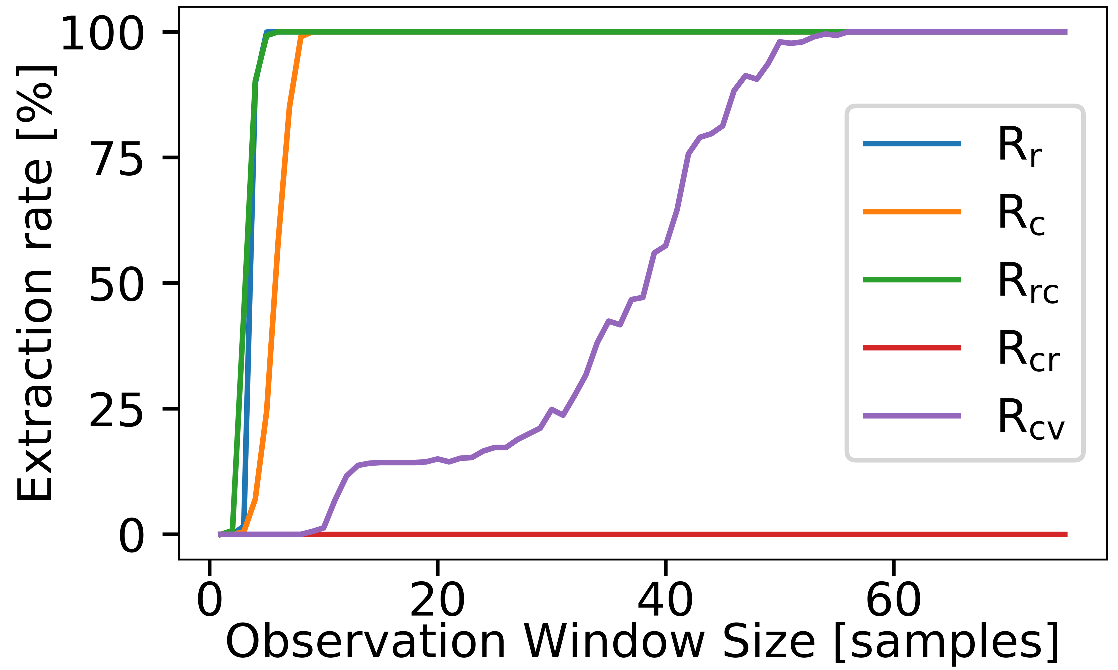
We chose an observation window size of ten symbols to ensure that we will always extract the rules from Rc. However, the choice of observation window meant that we would also retrieve some instances of rules from Rcv and Rrc. Rules in Rcv had no impact on process separation and could be ignored. Therefore, the separation task was achieved by removing the Rrc rules from the final set using the rule filters. We found that the confidence threshold filter always correctly separated the symbols into generating processes. The Bayesian factor filter only selected the chain rules and therefore no symbols from are grouped. Finally, the best confidence per conclusion filter failed to separate symbols into two generating processes, because symbol 10 is always associated as conclusion with a symbol.
6 Census and Chemical Exposure Database Mining
In this experiment, we illustrate BRM for database mining and analyse the differences in results retrieved by BRM and FRM.
6.1 Methodology
We used the publicly available dataset from Huang et al. [22]. The dataset comprises US census tract information from the American Community Survey (ACS) 5-year summary files for the 2010 to 2014 period. Moreover, the dataset contained chemical exposure data generated from the 2011 National-Scale Air Toxics Assessment (NATA), specifically, air pollutant exposure concentration. Huang et al. reported results for two mining scenarios: (1) mining rules using the socioeconomic variables as premises and chemical exposure variables as conclusions (SC), and (2) mining rules within the socioeconomic dataset (SS). Huang et al. used minimum-support of and lift as thresholds for FRM-based rule selection. We replicated their findings with an exhaustive search FRM algorithm and compared the extracted rules to BRM results.
We followed Huang et al.’s categorisation of variables in the dataset. Socioeconomic scores were divided into deciles, chemical variables into quartiles, and age group used the ranges: [0–20], (20–30], (30–35], (35–38], (38–40], (40–50], (50–150]. The poverty score was computed as the percentage of population per track that had a ratio between income and poverty level below 1.5. Additionally, deciles seven through ten were combined. Education score was calculated as the population percentage per track that had demonstrated education beyond high school level. Deciles eight through ten of the education score where merged. Finally, the race score was calculated as the percentage of the non-white population per track.
6.2 Evaluation
We chose Huang et al. [22] as a reference because they analysed the problem and provided relevance criteria to interpret the extracted rules in their field. We reasoned that if BRM extracted rules that were in Huang et al.’s selection, then, BRM’s increasing belief approach can extract relevant rules.
In our preliminary test, we noticed that BRM was very selective and only extracted five rules. Therefore, we used the Selector to control BRM’s sensitivity (see Eq. 2). We performed a parametric search on the Selector , using 200 equidistant samples from the range , to find the value that allowed BRM to extract the missing rules from Huang et al.’s SC and SS scenarios.
For any new-found rule, we computed the odds-ratio (OR), with a 95% confidence interval (CI). The CI was calculated using 10000 runs of bootstrapping, following Huang et al. [22]’s evaluation of rule relevance.
6.3 Results
Table I lists the mined rules from Huang et al. [22] SC scenario, with their respective BRM’s selector value , support, and probability of premise given the conclusion . Using BRM’s default behaviour, i.e., with , we extracted only five rules. To extract all rules from Huang et al., BRM required a selector lower than .
| Rules | Selector | Support | |
|---|---|---|---|
| Race score = 1 Diesel = Q1 | 1.000 | 0.144 | 0.578 |
| Race score = 1 Butadiene = Q1 | 1.000 | 0.142 | 0.585 |
| Race score = 1 Toluene = Q1 | 1.000 | 0.138 | 0.566 |
| Race score = 1 Benzene = Q1 | 1.000 | 0.130 | 0.535 |
| Race score = 1 Acetaldehyde = Q1 | 1.000 | 0.126 | 0.517 |
| Age group = 40–50 Diesel = Q1 | 0.995 | 0.124 | 0.499 |
| Age group = 40–50 Butadiene = Q1 | 0.910 | 0.116 | 0.477 |
| Age group = 40–50 Toluene = Q1 | 0.874 | 0.114 | 0.467 |
| Age group = 40–50 Benzene = Q1 | 0.849 | 0.112 | 0.459 |
| Age group = 40–50 Acetaldehyde = Q1 | 0.769 | 0.106 | 0.436 |
| Race score = 1 Cyanide = Q3 | 0.754 | 0.110 | 0.431 |
| Race score = 1 Toluene = Q2 | 0.698 | 0.104 | 0.411 |
| Race score = 1 Diesel = Q2 | 0.683 | 0.102 | 0.408 |
Tab. II lists mined association rules in the SS scenario. BRM found two out of the six rules reported by Huang et al. Additionally, BRM found three rules, highlighted in Tab. II, that did not pass the minimum-support and lift criteria from Huang et al. To retrieve all six rules from Huang et al., BRM required a selector and extracted 41 additional rules.
| Rules | Selector | Support | |
|---|---|---|---|
| Race score = 1 Age group = 40–50 | 1.000 | 0.172 | 0.516 |
| Age group = 40–50 Race score = 1 | 1.000 | 0.172 | 0.528 |
| Race score = 1 Poverty score = 2 | 0.764 | 0.111 | 0.434 |
| Poverty score = 2 Race score = 1 | 0.513 | 0.111 | 0.340 |
| Age group = 40–50 Poverty score = 2 | 0.749 | 0.110 | 0.430 |
| Poverty score = 2 Age group = 40–50 | 0.487 | 0.110 | 0.329 |
| Poverty score = 1 Education score = 8 | 1.000 | 0.038 | 0.623 |
| Poverty score = 1 Education score = 7 | 1.000 | 0.034 | 0.510 |
| Race score = 1 Age group = 50–150 | 1.000 | 0.015 | 0.725 |
The conditional probability , i.e., the premise probability given that the conclusion was observed, describes the ratio of conclusion observations associated to the premise. Thus, a higher reflects the rule’s relevance, because a larger portion of the conclusions can be explained by the premise. The rules extracted exclusively by BRM show that the conclusions are associated between 51% to 73% with their respective premises in the SS scenario. Whereas for FRM based rules, the maximum association is 52% for the SS scenario. Therefore, BRM rules would have a higher chance of correctly predicting the conclusion when the premise is observed. In the SC scenario, the best association is 59% for both BRM and FRM.
Fig. 3 illustrates the selector’s effect on the total number of extracted rules for both database mining scenarios. The Selector had an exponential effect on the exclusion of rules in both scenarios. The SC scenario converged to the Huang et al.’s rules, while the SS scenario always extracted additional rules.
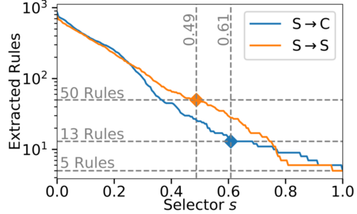
With there were no conjunctive premise candidates in ether scenarios. In SC, even after setting , there were no resulting conjunctive rules that pass the increasing belief criterion. In SS, the disjunctive conclusion rules Poverty score=1 Education score = (7 or 8), and Race score = 1Age group = 40–150, both have increasing belief with of 56% and 53% respectively. Therefore, rules with disjunctive conclusion suggest that the categories from Age group and Education score could be merged.
Tab. III shows the odds’ ratio (OR) and estimated 95% confidence interval (CI) for rules exclusively extracted by BRM in the SS scenario. The OR analysis showed that the new rules had higher OR than the rules from Huang et al, whose OR ranged from 1.75 to 3.56. Rules with increasing belief had the largest OR in both mining scenarios. Thus, BRM rules are more likely to appear in a repeat experiment, and therefore, BRM rules may be deemed more desirable.
| Rule | OR | Est. 95% CI | |
|---|---|---|---|
| Race score = 1 Age group = 40–50 | 3.56 | 3.45 | 3.68 |
| Age group = 40–50 Race score = 1 | 3.56 | 3.45 | 3.68 |
| Poverty score = 1 Education score = 8 | 11.18 | 10.49 | 11.94 |
| Poverty score = 1 Education score = 7 | 6.74 | 6.35 | 7.17 |
| Race score = 1 Age group = 50–150 | 5.68 | 5.10 | 6.39 |
7 Rehabilitation Routine Mining
We show how BRM can be used to interpret patient behaviour during stays at a day care rehabilitation centre. We compare BRM and FRM for classifying patients into physically active and sedentary groups. However, we observed that FRM represents the cohort’s average behaviour and thus fails to assign patients to groups.
| No Filter | Bayesian Factor | Confidence 0.5 | Best Confidence | |
|---|---|---|---|---|
|
BRM |
\Centerstack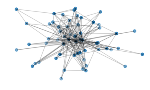
|
\Centerstack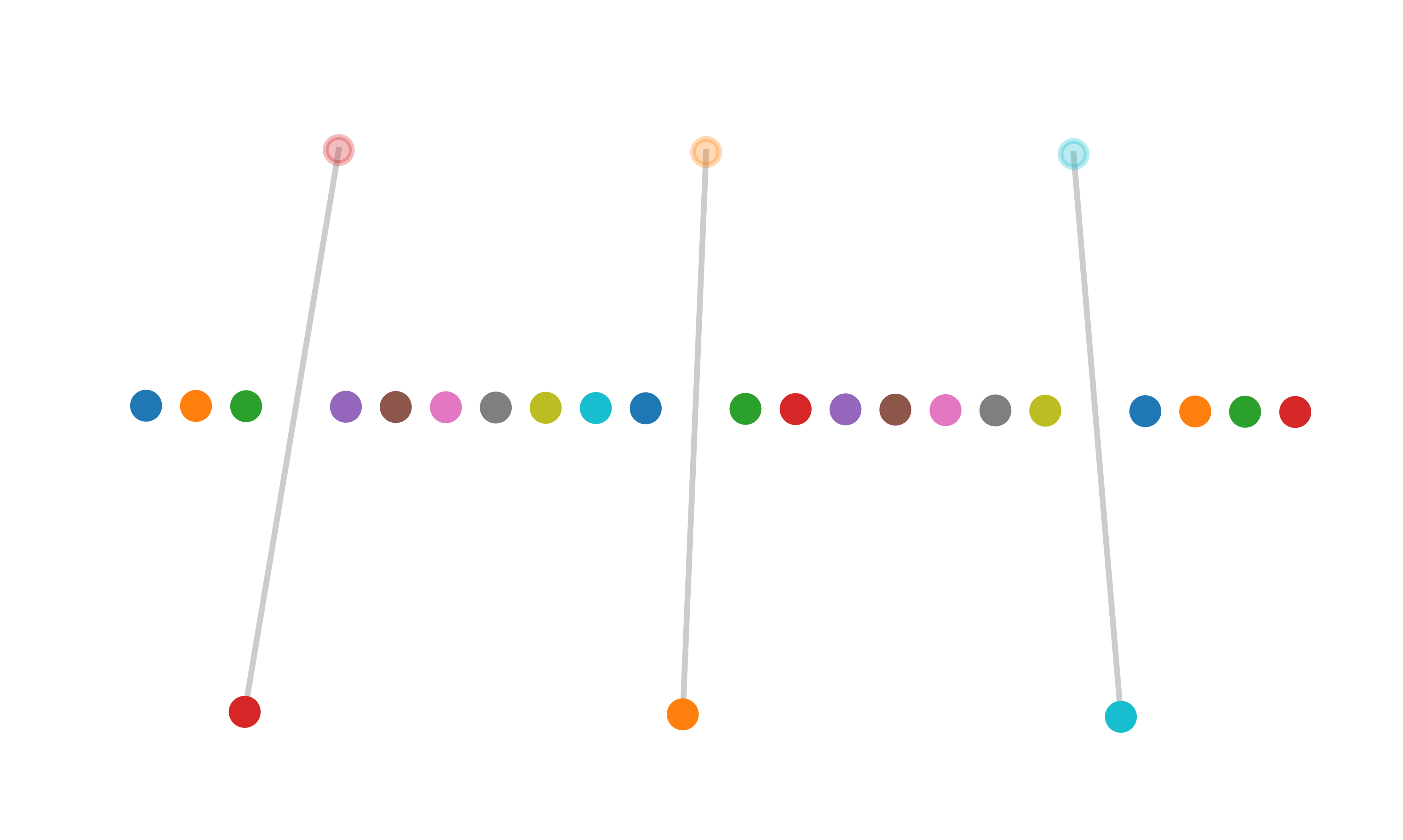
|
\Centerstack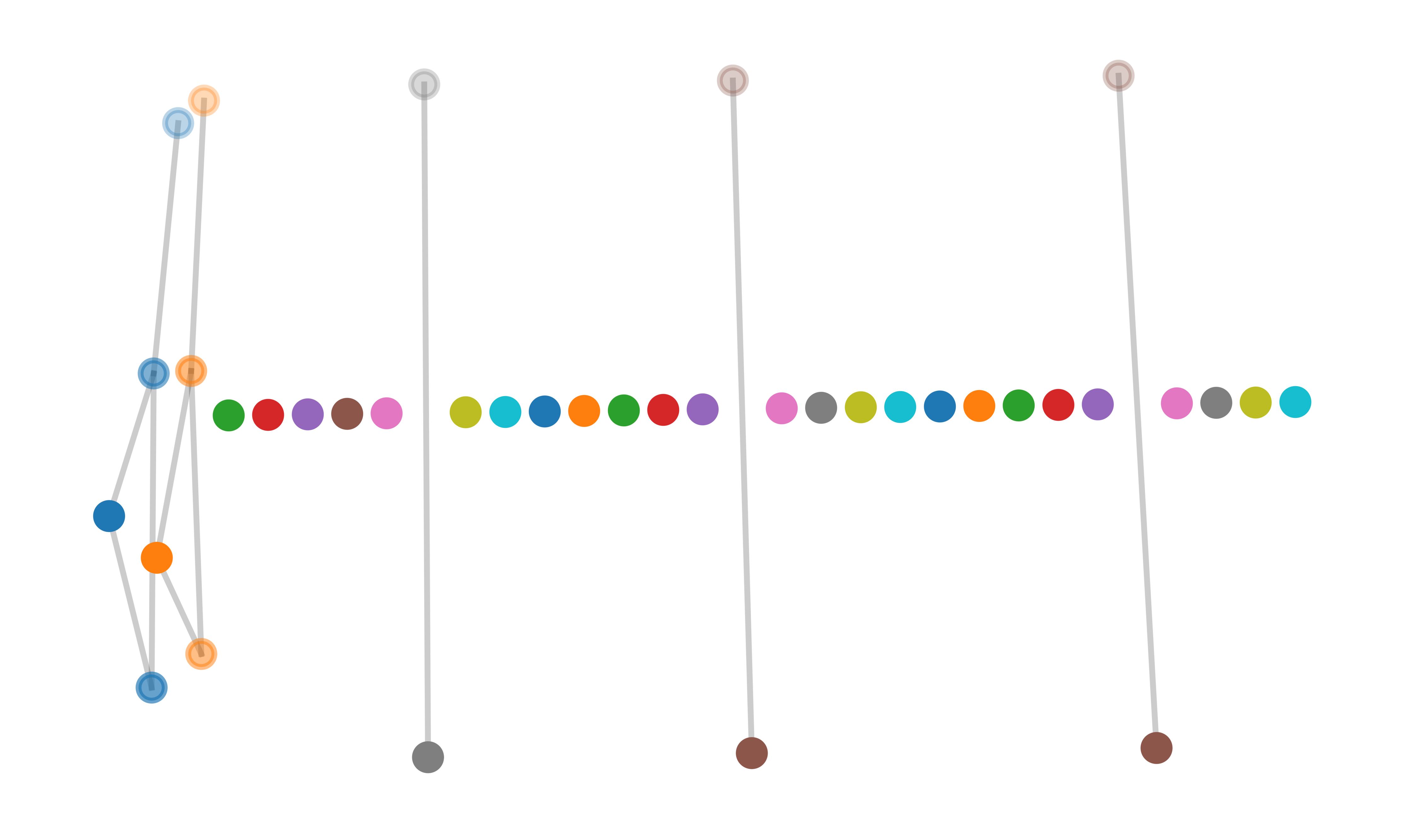
|
\Centerstack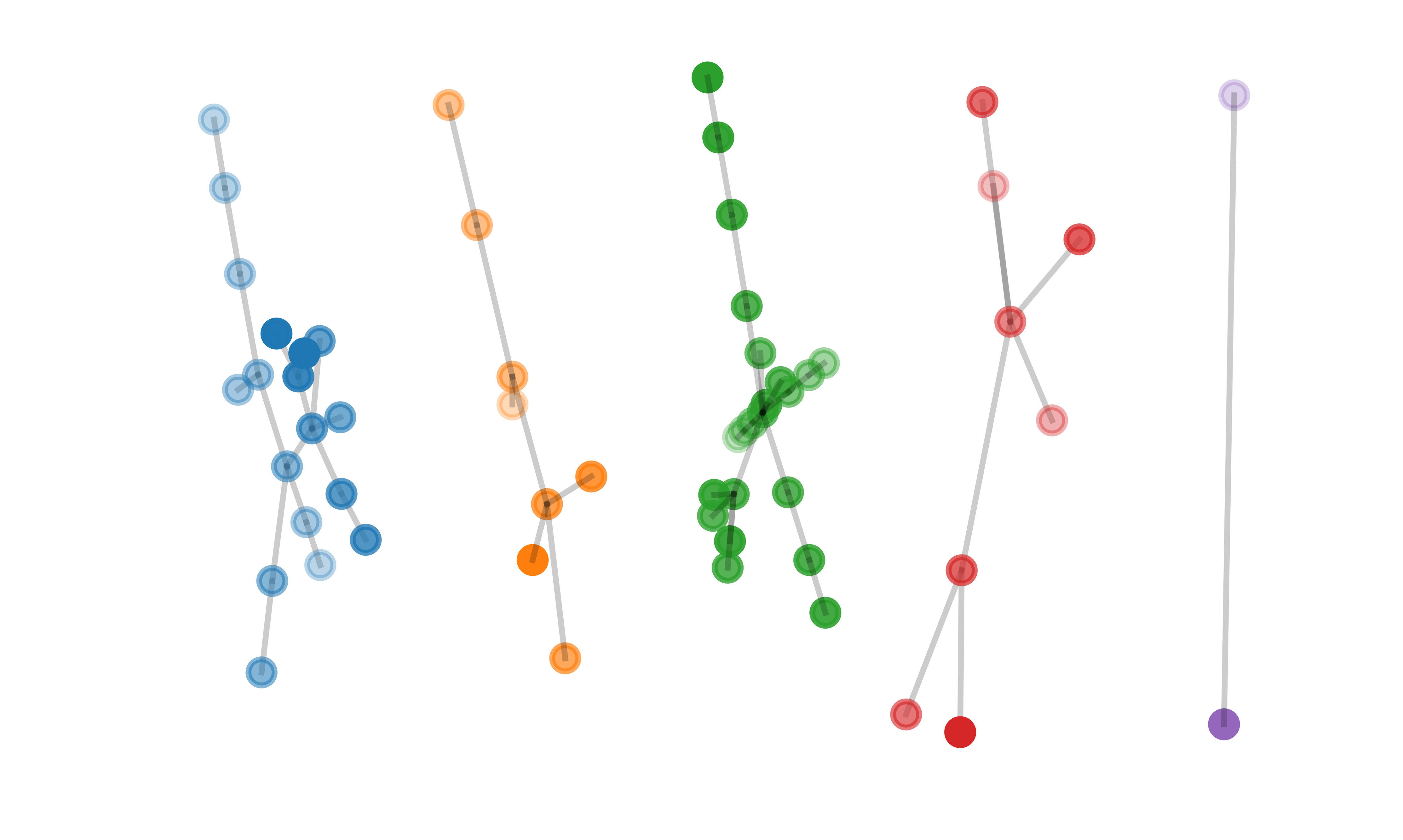
|
|
FRM |
\Centerstack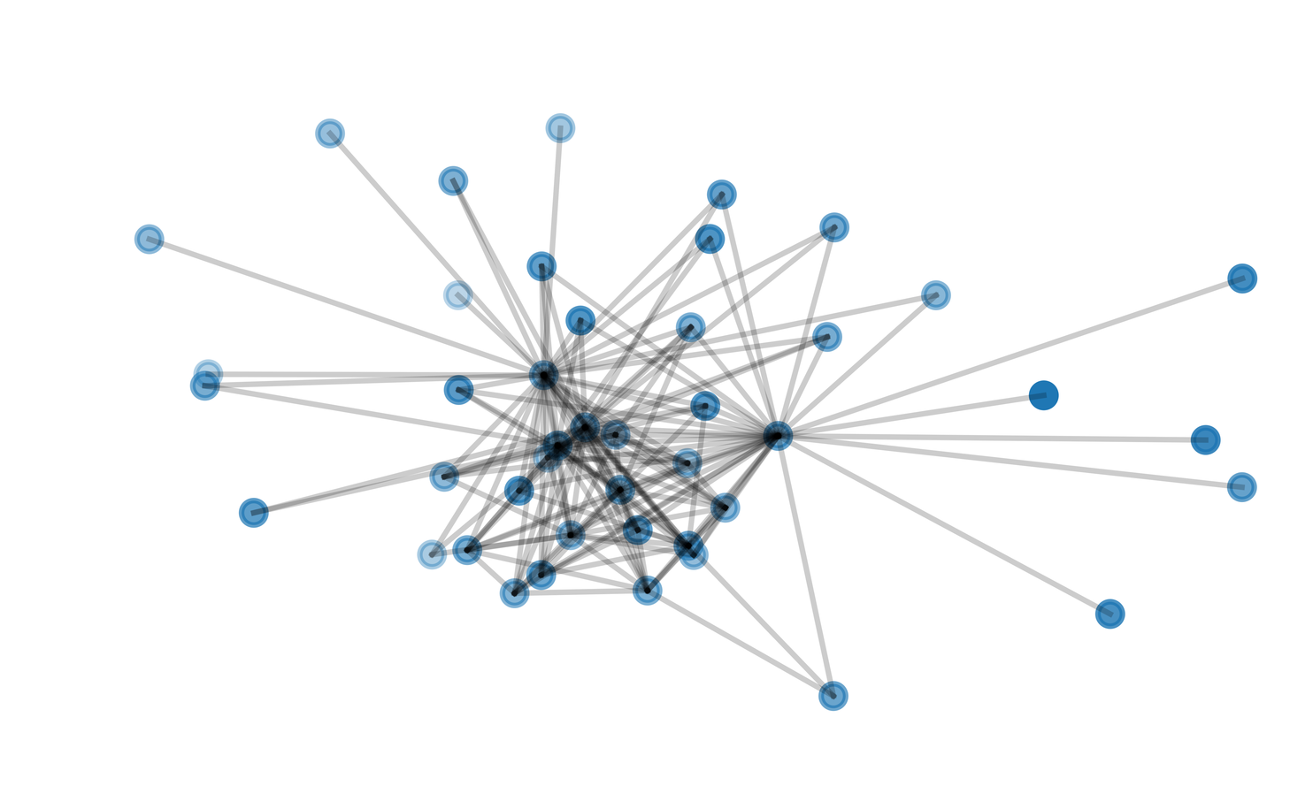
|
\Centerstack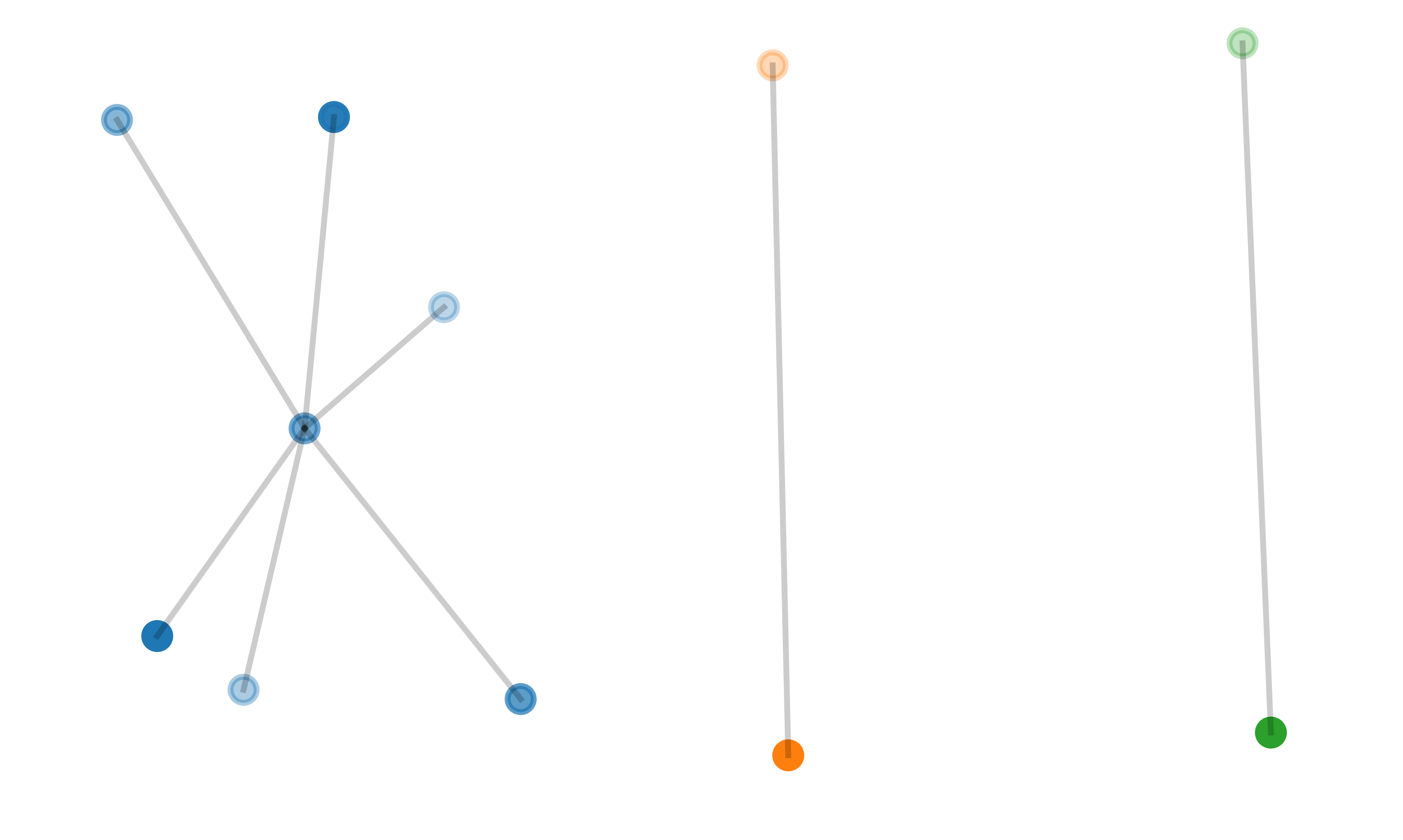
|
\Centerstack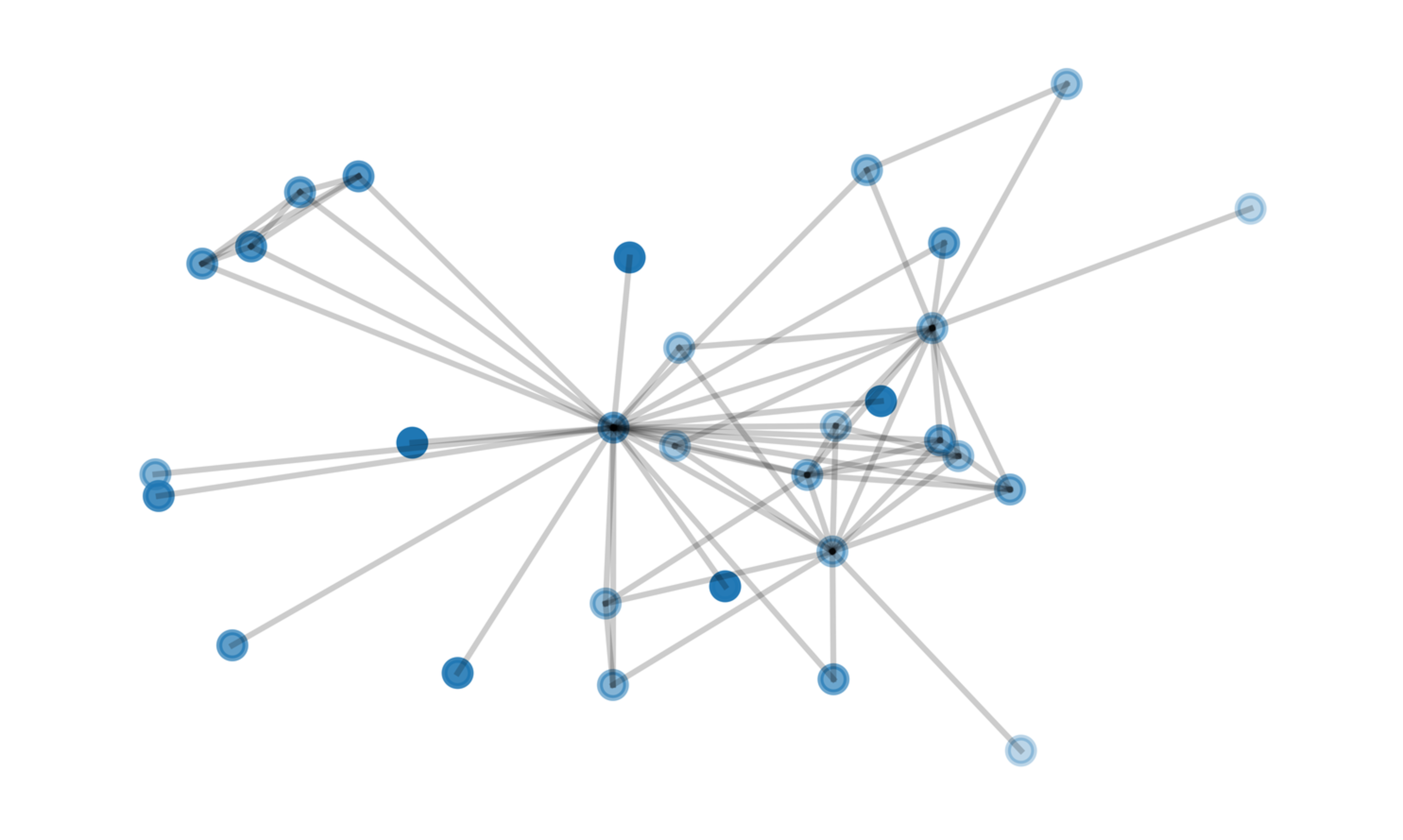
|
\Centerstack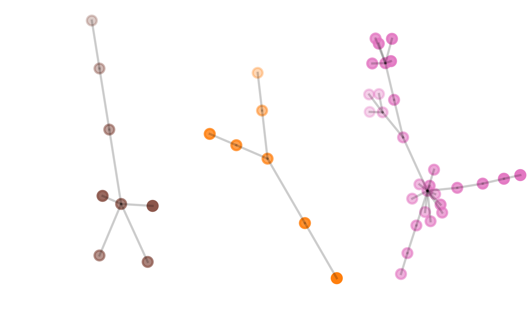
|
7.1 Methodology
For the rehabilitation routine mining experiment, we used activity labels from the longitudinal stroke rehabilitation study of Derungs et al. [23]. The study was approved of the Swiss cantonal Ethics committee of the canton Aargau, Switzerland (Application number: 2013/009). There were eleven patients in the study, aged 34 to 75 years, five female, and four used a wheelchair. In addition, we used data from a patient excluded from the original rehabilitation study [23], for a total of 12 patients.
Patients visited the day care centre for approximately three days per week over three months to participate in individual and group training sessions, socialise with others, and follow personal activity preferences. Some training sessions available to patients were physiotherapy, ergotherapy, and training in the gym. Patients performed activities of daily living, including walking, eating and drinking, setting the table, writing, and making coffee. Behaviour of each patient was recorded for up to eight hours on 10 days at the centre by two observers accompanying patients. In addition, body motion was recorded using inertial sensors attached to wrists, upper arms, and tight positions. During the observation time, the examiners annotated patient activities using a customised annotation tool on a smartphone, resulting in a total of 16226 activity labels. Therapists scored patients for their ability to execute activities of daily living independently using the Extended Barthel Index (EBI) [24]. The EBI consists of 16 categories. Each category receives a score within the range zero to four, where zero means that the patient requires full support, and four means the patient can live independently.
We started by mining atomic rules from patient’s activity labels. Subsequently, we filtered the rules and created graphs. Each resulting independent subgraph was considered a routine, which was analysed by a study observer to assign a routine label. We observed that by removing an active patient from the mining dataset, the resulting routines would change with respect to the routines extracted using all patients. Removing a sedentary patient had no effect in the resulting routines. Therefore, we classified patients into physically active or sedentary groups by removing the patient’s data from the mining dataset. We refer to the patient classification method as patient exclusion process (PEP).
7.2 Evaluation
For BRM, we used the default Selector value and an observation window of 20 minutes. For FRM, we used an exhaustive search algorithm with a minimum-support threshold of 0.0038. The minimum-support threshold value was chosen to obtain the same number of rules as for BRM. Both methods were set to extract atomic rules only, used label names as symbols, and their start times as symbol timestamp.
We evaluated each mining method by submitting their extracted rules to the same post-processing two stage procedure: (1) rule filtering, and (2) graph-based routine classification. In the rule filtering stage, we evaluated three filtering methods: Bayesian factor (Eq. 5), confidence threshold of 0.5 and best confidence per conclusion. With the retained rules, we built a graph and extracted routines as independent subgraphs. For each mining method, we chose a filter for the post-processing procedure that provided a balance between activity label count per graph and the number of independent graphs. Subsequently, we compared the mining methods with their respective post-processing procedures to classify patients into physically active, and sedentary groups using PEP.
Based on the type of the majority of activities in the routine, a study observer named BRM routines as socialising, eating, using the phone, intense and balance training. Whereas, FRM routines were named mobility, eating, and cognitive-motor training. We observed that FRM routines lacked emphasis on activities related to socialising.
7.3 Results
The No Filter column in Fig. 4 shows the resulting graphs based on atomic rules extracted by BRM and FRM methods. Activities in both graphs are hyperconnected, i.e., multiple edges connect activities. However, for FRM, there are nodes with one edge. FRM rules do not describe the flow from one activity to another, but rather, the associations of repeating events, e.g., repetitions of an exercise. In contrast, BRM looks for successive activities, and the respective low count of activity transitions vs exercise repetitions does not affect the rule selection. For both mining algorithms, the hyperconnected graph yielded no useful routine information.
We evaluated the effect of rule filtering on graph creation. With a Bayesian factor , BRM mined rules focus mostly on self-referencing activities, e.g., , resulting in single activity subgraphs. In contrast, the Bayesian factor filter removed most of the FRM rules. The resulting subgraphs had too few activities to consider them as routines. For FRM rules, the confidence filter reduced the graph size, but it was unable to create independent subgraphs. However, with BRM rules, the confidence filter selected many self-referencing rules. The confidence filter was able to create two more subgraphs than the Bayesian factor, containing four activities each. However, there were too many single activity subgraphs to consider the split as routines. We obtained the best balance between the number of subgraphs and activities per graphs using the best confidence per conclusion filter. After filtering, BRM-mined rules yielded five routines, whereas FRM-mined rules yielded only three. Fig. 4 illustrates the resulting subgraphs for each mining algorithm and rule filtering method.
| All Patients | Without Patient ID 9 | Without Patient ID 10 | Without Patient ID 12 | |
|
BRM |
\Centerstack
|
\Centerstack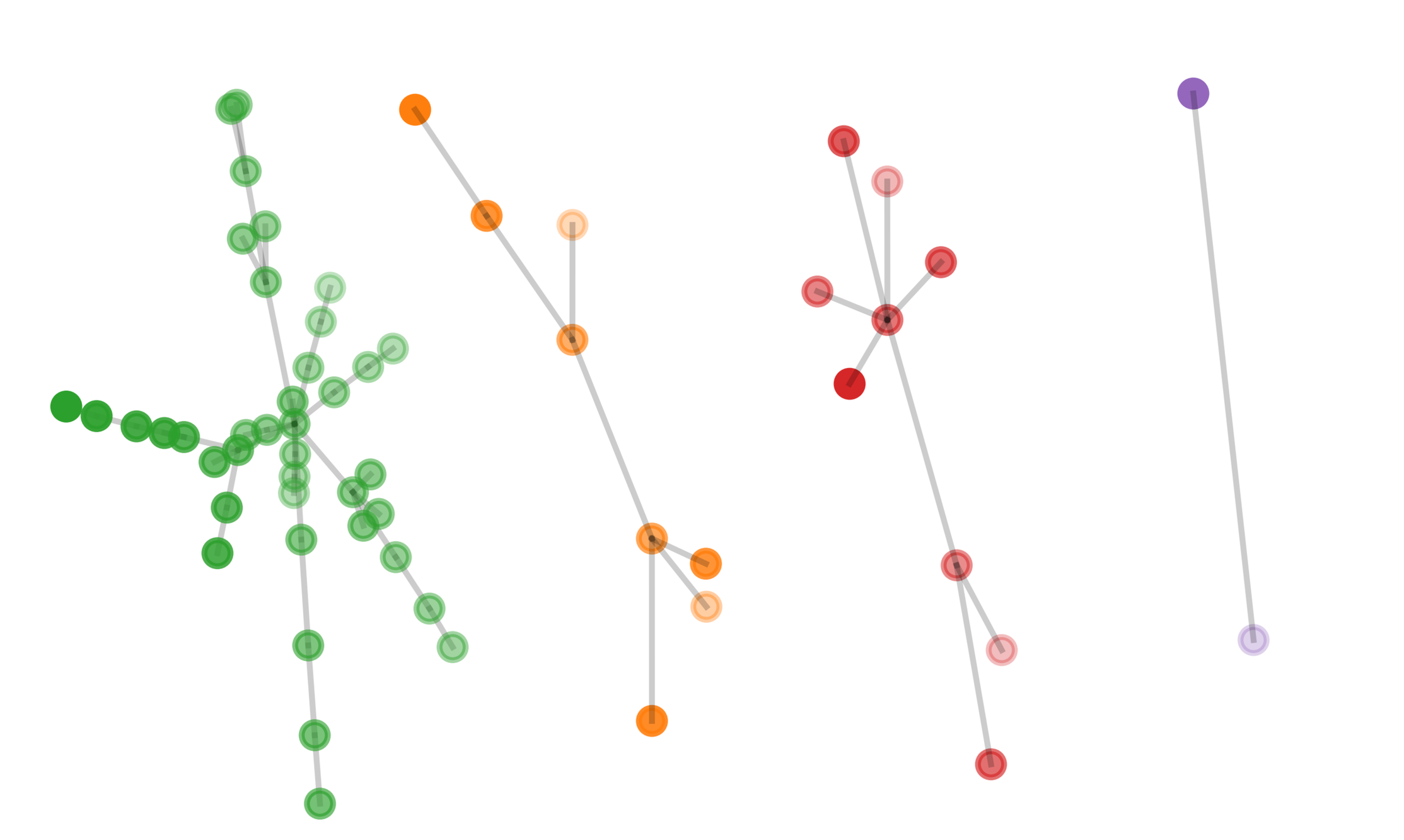
|
\Centerstack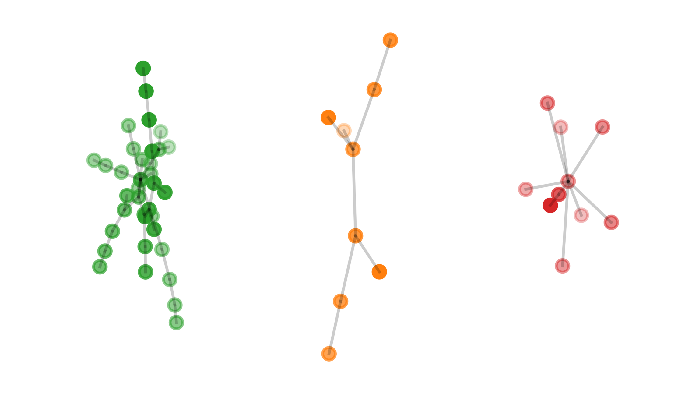
|
\Centerstack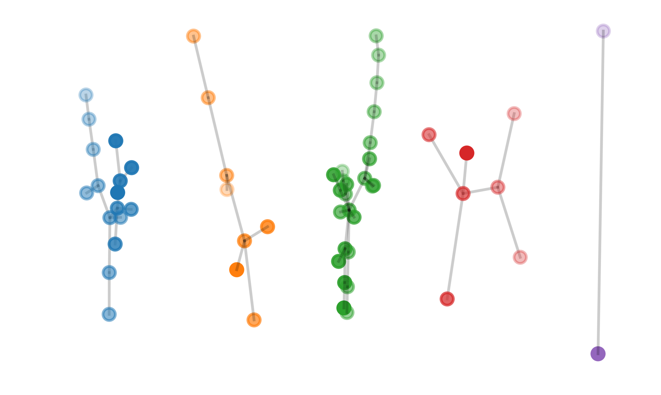
|
|
FRM |
\Centerstack
|
\Centerstack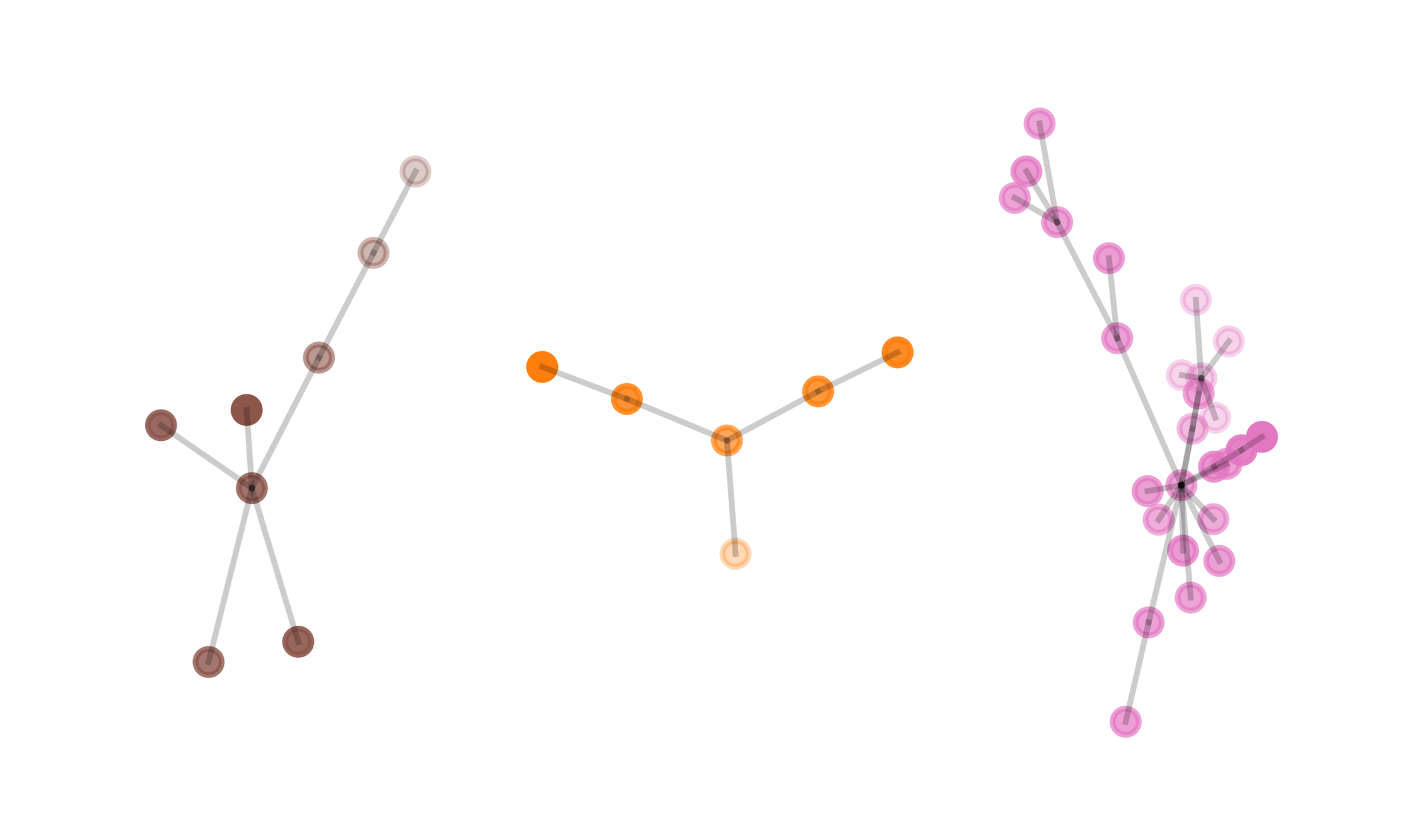
|
\Centerstack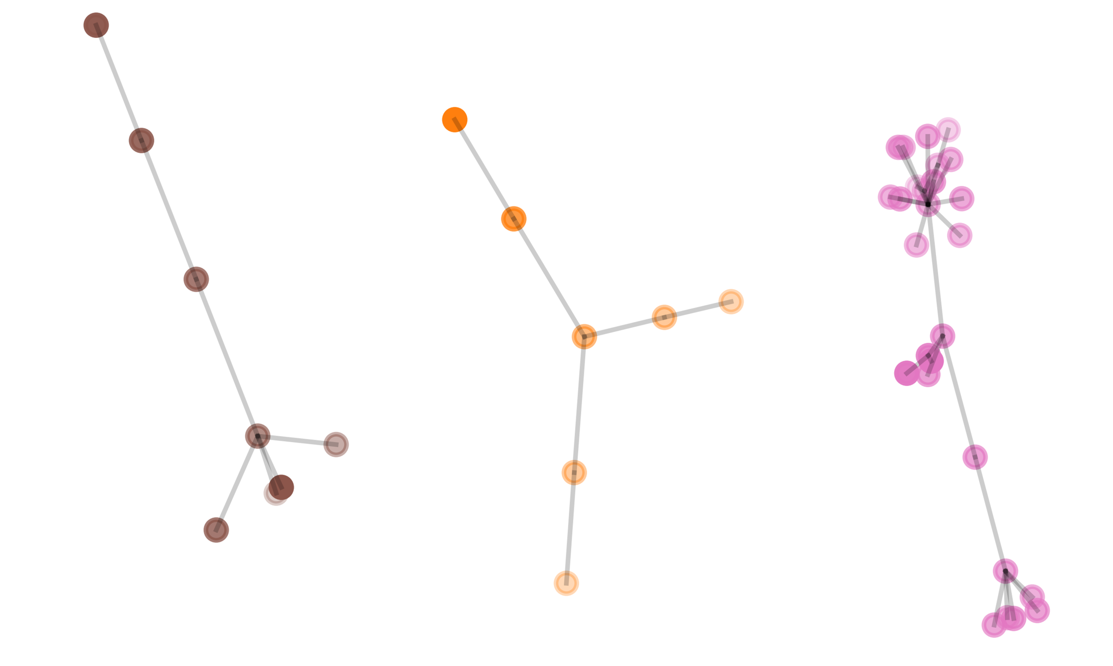
|
\Centerstack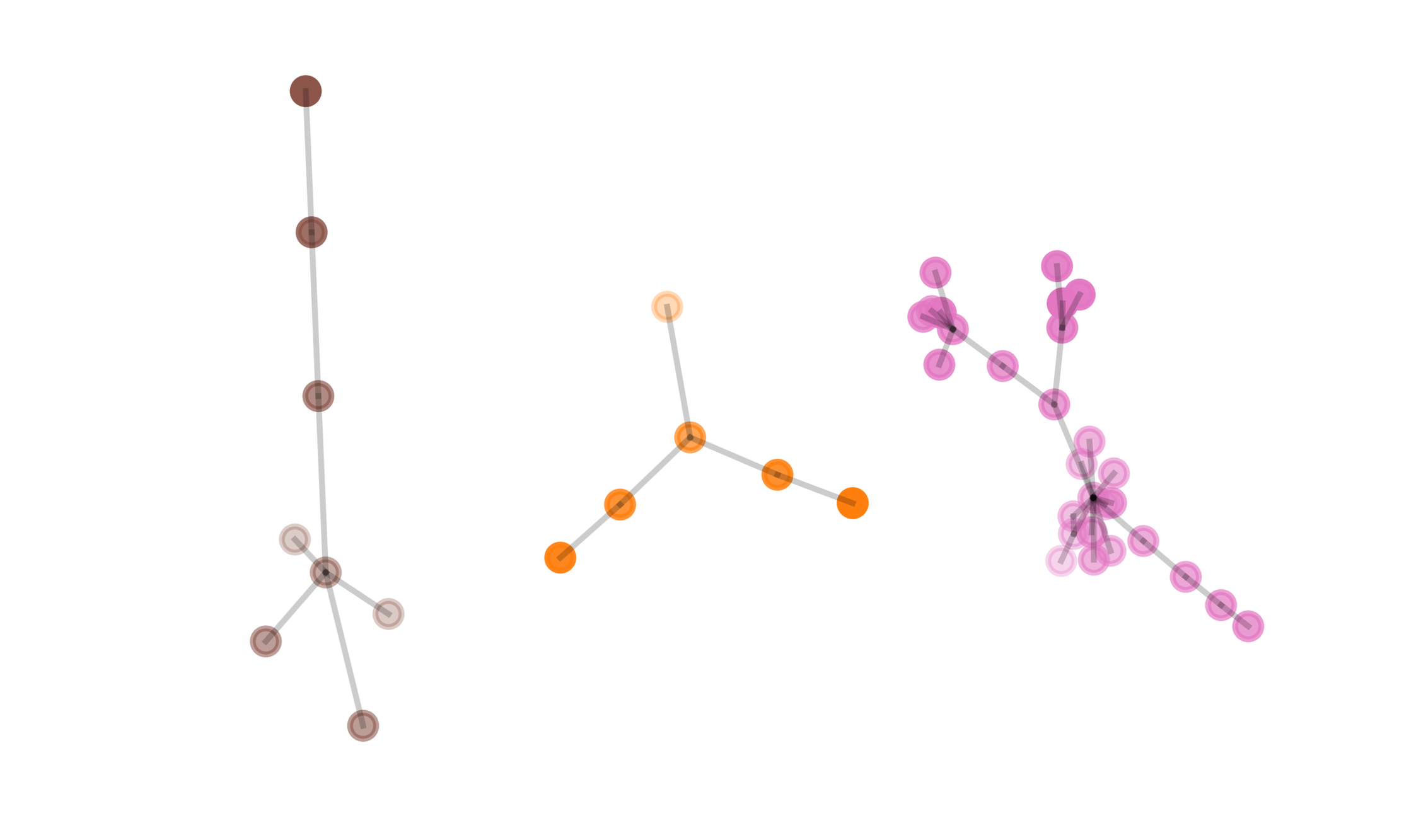
|
Fig. 5 illustrates an example of the changes in routine graphs when removing patients with active and sedentary behaviour. In the Appendix, we have included the complete set of graphs for the PEP analysis. For both mining algorithms, when removing one patient, the routine’s activity composition varied, but the assignment of routine labels by the study observer did not vary. In the PEP analysis, using the best confidence per conclusion filter, BRM mined routines that grouped patients into physically active and sedentary groups. We observed that the removal of patient ID 10 made the routine using a phone disappear. Apparently, the patient frequently used the phone. We found that the physically active group contained patient IDs 2,4,6,9, and 10. The physically active group refers to patients following their rehabilitation schedule closely. No relation to activity intensity or EBI score was found. The active patient group consisted of one wheelchair rider, patients with different EBI starting points, and some patients, where the EBI score did not change. When a patient from the active group was removed, the extracted routine number reduced to four and socialising was always missing. The result appears counter-intuitive as the sedentary group has been likely involved in socialising, but could be explained by the chosen 20 minute observation window, which causes BRM to focus on transitions between activities of at most 20 minute duration. Sedentary patients would perform individual activities for periods longer than 20 minutes. Therefore, their socialising activities would not be associated into rules.
For comparison, we performed PEP analysis for FRM-extracted routines using rules with the best confidence per conclusion. We found that the removal of any one patient did not affect the extracted routines. Therefore, FRM provided no further insight, and classifying patient’s into physical activity groups was not possible.
8 Conclusions
BRM’s parameters can be adjusted using process knowledge. Selector is a proportion of conclusions to consider, which does not dilute if the dataset size increases, and therefore can be calculated as the ratio of the expected rare and frequent symbol frequencies. The observation window size is determined using the transition times between events of interest. The prior does not play a role in rule selection. In contrast, most FRM-based methods use parameters that are difficult to define in terms of the processes or dataset properties.
The prior determines the rule’s final belief value. Therefore, comparisons of absolute belief values across datasets requires attention to the prior values used with each dataset. With this consideration, we do not propose belief as a stand-alone rule interest metric.
The first limitation of BRM is the sporadic association of frequent premises with infrequent conclusions into irrelevant rules. By using a filtering stage, we removed the irrelevant rules. However, we found that the filter of choice depends on the experiment. For example, in our proof-of-concept experiment, we used a confidence threshold to separate symbols into generating processes, and for the rehabilitation routine mining experiment, we used the best rule confidence per conclusion. We theorize that, in general, if the distributions of symbols in the dataset is not uniform and the mining task is to separate per underlying process, then the confidence threshold filter may be more useful to remove irrelevant rules, whereas best confidence per conclusion filter is better suited to extract transitions between symbols.
We believe that BRM rules provide meaningful insight, in particular on rarely, but consistently occurring relations, which may provide application experts with new hypotheses to investigate. For example, as seen in the SS scenario of the database mining experiment, BRM provided additional rules over FRM that hint to a predominantly white ageing population (Race score = 1 Age group 40-150), and to a correlation between low poverty score and high education levels (Poverty score = 1 Education score = 7 or 8).
In this paper, we presented an exhaustive search implementation of a BRM algorithm. Nevertheless, he optimisation strategies used for FRM could be adpated to BRM by replacing the minimum-support with increasing belief and the downward-closure property with Prop. 1 and Prop. 3.
BRM is not a replacement for FRM. The application should drive the choice of algorithm branch. If the application task is to extract symbol relationships from a single process, then, FRM is suitable. If instead, the task is to separate multiple process in the dataset, then BRM is suitable and may provide more insight over FRM. We summarise the difference between both branches as follows: FRM focuses on extracting rules that describe the commonalities between generating processes. In contrast, BRM looks for rules that describe each process.
The rehabilitation routine mining experiment illustrated the difference between both association rule mining branches. Routines mined with FRM did not change during PEP analysis. FRM mined routines that were common to the entire population. With BRM, the routines changed during PEP analysis, grouping patients into active and sedentary groups. Hence, FRM answers the question: what routines are commonly done by all patients?, and BRM answers the question: what types of patients are there?
In this paper, we defined increasing belief using the Bayes theorem recursively. We introduced the BRM branch to the association rule mining taxonomy, where rules are extracted using increasing belief, and presented an implementation of an exhaustive search BRM algorithm. We showed that BRM does not suffer from support dilution, and that BRM is capable of extracting rare rules from a dataset. The proof-of-concept and socioeconomic experiments illustrated how BRM extracted frequent and rare rules. In the rehabilitation routine mining experiment, we used BRM to mine rules, create routines, and group patients into active and sedentary groups. Only BRM rules provided patient grouping information.
Acknowledgments
We are thankful to the study participants and the clinicians at the Reha Rheinfelden. The authors thank Dr. Julia Seiter for supporting the study data recordings.
References
- [1] R. Agrawal, T. Imieliński, and A. Swami, “Mining Association Rules Between Sets of Items in Large Databases,” in Proceedings of the 1993 ACM SIGMOD International Conference on Management of Data, ser. SIGMOD ’93. New York, NY, USA: ACM, 1993, pp. 207–216.
- [2] L. I. Lopera Gonzalez and O. Amft, “Mining hierarchical relations in building management variables,” Pervasive Mob. Comput., vol. 26, pp. 91–101, Feb. 2016.
- [3] S. Liu and H. Pan, “Rare itemsets mining algorithm based on RP-Tree and spark framework,” AIP Conference Proceedings, vol. 1967, no. 1, p. 040070, May 2018.
- [4] M. Bayes and M. Price, An Essay towards Solving a Problem in the Doctrine of Chances. By the Late Rev. Mr. Bayes, F. R. S. Communicated by Mr. Price, in a Letter to John Canton, A. M. F. R. S. Royal Society of London, Jan. 1763.
- [5] V. Beiranvand, M. Mobasher-Kashani, and A. Abu Bakar, “Multi-objective PSO algorithm for mining numerical association rules without a priori discretization,” Expert Syst. Appl., vol. 41, no. 9, pp. 4259–4273, 2014.
- [6] F. Padillo, J. Luna, F. Herrera, and S. Ventura, “Mining association rules on Big Data through MapReduce genetic programming,” Integr. Comput.-Aided Eng., vol. 25, no. 1, pp. 31–48, Dec. 2017.
- [7] L. I. Lopera Gonzalez, “Mining Functional and Structural Relationships of Context Variables in Smart-Buildings,” Ph.D. dissertation, Universität Passau, Passau, 2018.
- [8] P.-N. Tan, M. Steinbach, and V. Kumar, Introduction to Data Mining. Addison-Wesley, 2005.
- [9] G. I. Webb, “OPUS: An Efficient Admissible Algorithm for Unordered Search,” 1, vol. 3, pp. 431–465, Dec. 1995.
- [10] ——, “Efficient Search for Association Rules,” in Proceedings of the Sixth ACM SIGKDD International Conference on Knowledge Discovery and Data Mining, ser. KDD ’00. New York, NY, USA: ACM, 2000, pp. 99–107.
- [11] R. Agrawal and R. Srikant, “Fast algorithms for mining association rules in large databases,” in Proceedings of the 20th International Conference on Very Large Data Bases, ser. VLDB ’94. San Francisco, CA, USA: Morgan Kaufmann Publishers Inc., 1994, pp. 487–499.
- [12] M. J. Zaki, “Scalable algorithms for association mining,” IEEE Trans. Knowl. Data Eng., vol. 12, no. 3, pp. 372–390, May 2000.
- [13] S. Bashir, Z. Jan, and A. R. Baig, “Fast Algorithms for Mining Interesting Frequent Itemsets without Minimum Support,” arXiv:0904.3319 [cs], 2009.
- [14] Y. Djenouri, D. Djenouri, A. Belhadi, P. Fournier-Viger, and J. C.-W. Lin, “A new framework for metaheuristic-based frequent itemset mining,” Appl Intell, vol. 48, no. 12, pp. 4775–4791, Dec. 2018.
- [15] I. Tahyudin and H. Nambo, “The Combination of Evolutionary Algorithm Method for Numerical Association Rule Mining Optimization,” in Proceedings of the Tenth International Conference on Management Science and Engineering Management, ser. Advances in Intelligent Systems and Computing, J. Xu, A. Hajiyev, S. Nickel, and M. Gen, Eds. Springer Singapore, 2017, pp. 13–23.
- [16] M. Guillame-Bert and J. L. Crowley, “Learning temporal association rules on symbolic time sequences,” in Proceedings of the 4th Asian Conference on Machine Learning, ACML 2012, Singapore, Singapore, November 4-6, 2012, 2012, pp. 159 – 174.
- [17] X. Yan, C. Zhang, and S. Zhang, “Genetic algorithm-based strategy for identifying association rules without specifying actual minimum support,” Expert Syst. Appl., vol. 36, no. 2, pp. 3066–3076, 2009.
- [18] S. Brin, R. Motwani, and C. Silverstein, “Beyond Market Baskets: Generalizing Association Rules to Correlations,” in Proceedings of the 1997 ACM SIGMOD International Conference on Management of Data, ser. SIGMOD ’97. New York, NY, USA: ACM, 1997, pp. 265–276.
- [19] S. Brin, R. Motwani, J. D. Ullman, and S. Tsur, “Dynamic Itemset Counting and Implication Rules for Market Basket Data,” in Proceedings of the 1997 ACM SIGMOD International Conference on Management of Data, ser. SIGMOD ’97. New York, NY, USA: ACM, 1997, pp. 255–264.
- [20] L. Liu, S. Wang, Y. Peng, Z. Huang, M. Liu, and B. Hu, “Mining intricate temporal rules for recognizing complex activities of daily living under uncertainty,” Pattern Recognition, vol. 60, pp. 1015–1028, Dec. 2016.
- [21] V. Srinivasan, C. Koehler, and H. Jin, “RuleSelector: Selecting Conditional Action Rules from User Behavior Patterns,” Proc ACM Interact Mob Wearable Ubiquitous Technol, vol. 2, no. 1, pp. 35:1–35:34, Mar. 2018.
- [22] H. Huang, R. Tornero-Velez, and T. M. Barzyk, “Associations between socio-demographic characteristics and chemical concentrations contributing to cumulative exposures in the United States,” J. Expo. Sci. Environ. Epidemiol., vol. 27, no. 6, pp. 544–550, Dec. 2017.
- [23] A. Derungs, C. Schuster-Amft, and O. Amft, “Longitudinal Walking Analysis in Hemiparetic Patients Using Wearable Motion Sensors: Is There Convergence Between Body Sides?” Front. Bioeng. Biotechnol., vol. 6, 2018.
- [24] M. Prosiegel, S. Böttger, T. Schenk, N. König, M. Marolf, C. Vaney, C. Garner, and A. Yassouridis, “Der erweiterte Barthel-Index (EBI)–eine neue Skala zur Erfassung von Fähigkeitsstörungen bei neurologischen Patienten,” Neurol Rehabil, vol. 1, pp. 7–13, 1996.
![[Uncaptioned image]](/html/1912.06432/assets/figures/lopera_luis.jpg) |
Luis Ignacio Lopera González received the MSc. degree in Electronic engineering and computer science from Los Andes University, Bogotá, Colombia, in 2005 and the Dr. rer. nat. degree from the University of Passau, Passau, Germany in 2018. He is currently working at the Chair of Digital Health at the Friedrich-Alexander University Erlangen-Nürenberg, Erlangen, Germany. His current research interest include rule mining algorithm development, and self commissioning systems in medical applications. |
![[Uncaptioned image]](/html/1912.06432/assets/figures/derungs_adrian.jpg) |
Adrian Derungs received the MSc. degree in Biomedical Engineering from the University of Bern, Bern, Switzerland in 2012. He is currently working toward the PhD degree with the Chair of Digital Health at the Friedrich-Alexander University Erlangen-Nürnberg, Erlangen, Germany. His current research interest include, wearable sensor technology and computing, machine learning, biomechanics and biomarker personalisation, and the digitalisation of healthcare. |
![[Uncaptioned image]](/html/1912.06432/assets/figures/amft-oliver.jpg) |
Oliver Amft received the Dipl.-Ing. (M.Sc.) from Chemnitz Technical University in 1999 and the Dr. sc. ETH (Ph.D.) from ETH Zurich in 2008, both in Electrical Engineering and Information Technology. In 2011, he obtained the university teaching qualification from TU Eindhoven. Until 2004, he was a R&D project manager with ABB, Inc. Oliver Amft was an assistant professor at TU Eindhoven between 2009 and 2013, tenured since 2011. In 2014, he was appointed full professor and established the Chair of Sensor Technology at University of Passau, Faculty of Computer Science and Mathematics. Since 2017, Oliver Amft is a full professor and director of the Chair of Digital Health at Friedrich-Alexander University Erlangen-Nürnberg. |
| BRM | FRM | |
| All Patients |
\Centerstack
|
\Centerstack
|
| Without user 01 |
\Centerstack
|
\Centerstack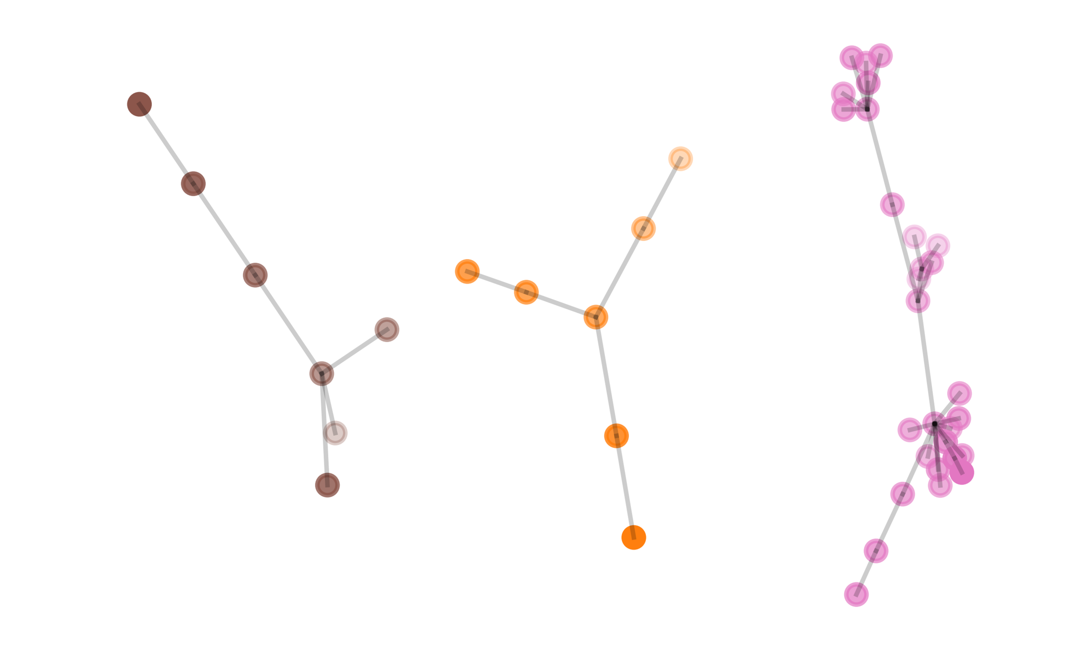
|
| Without user 02 |
\Centerstack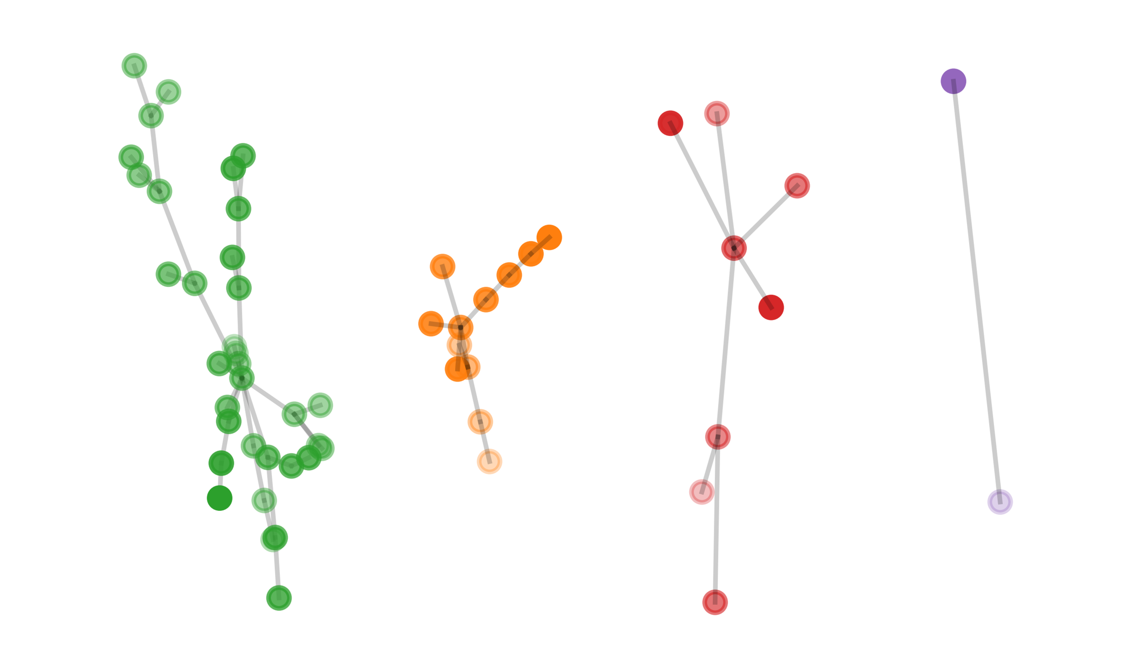
|
\Centerstack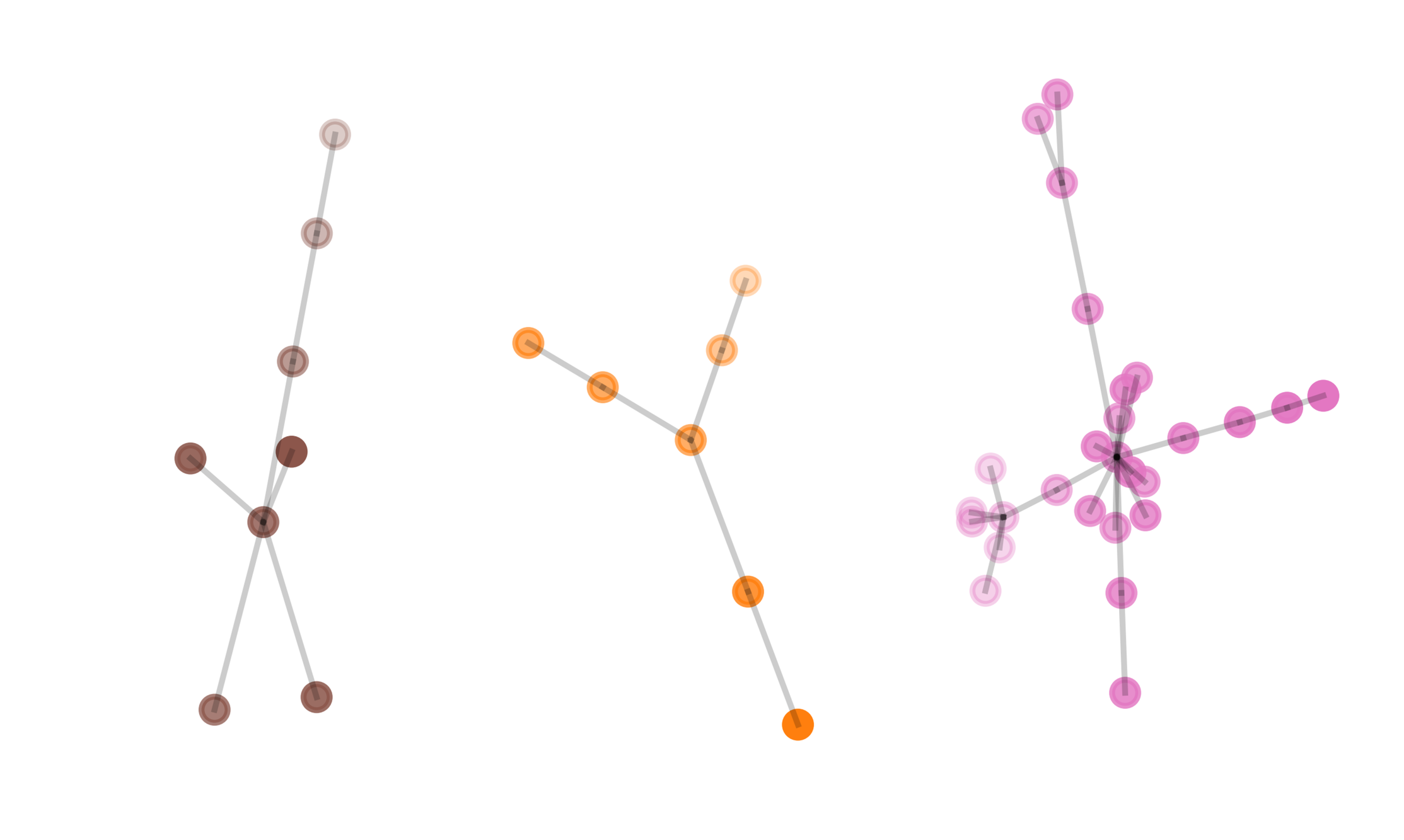
|
| BRM | FRM | |
| Without user 03 |
\Centerstack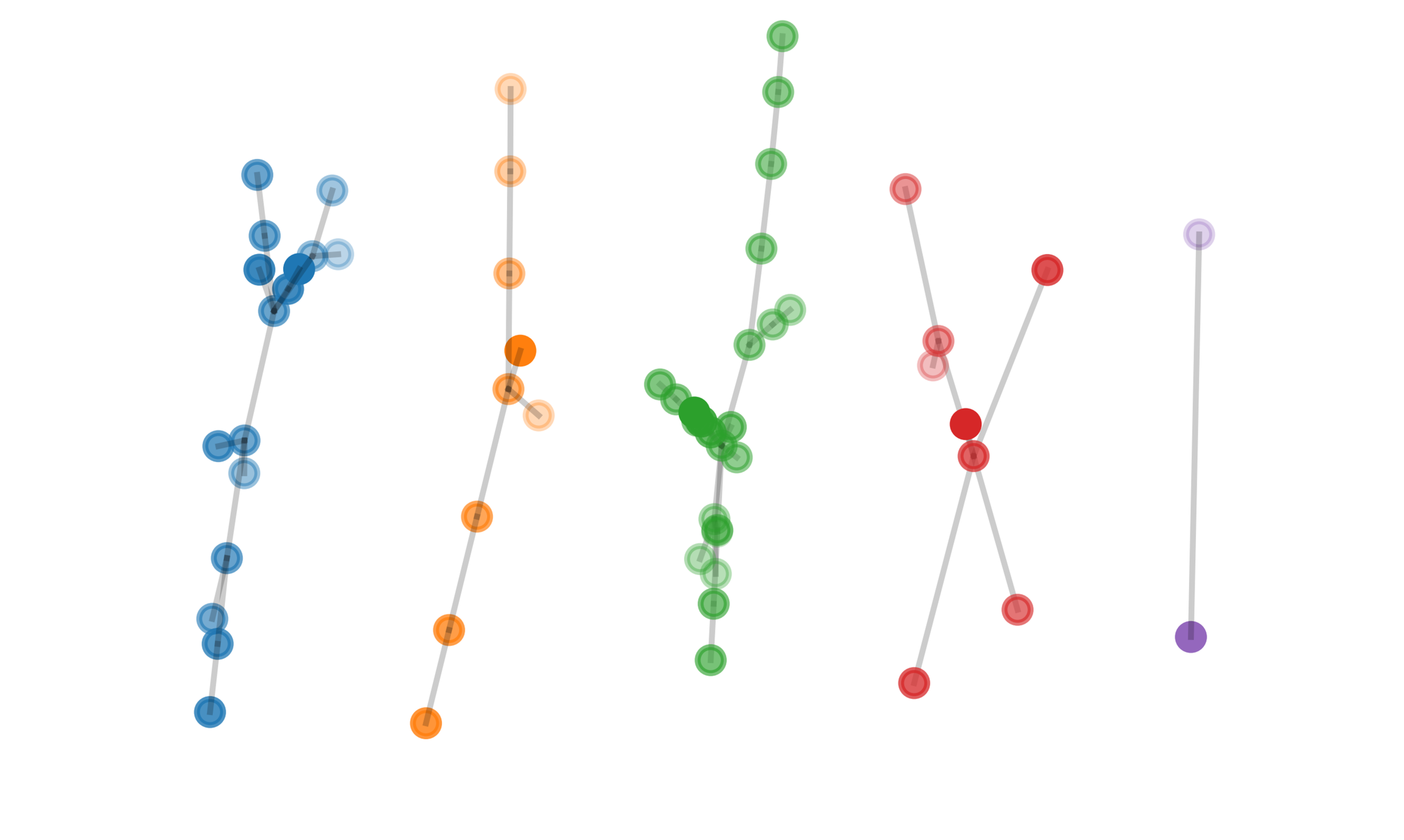
|
\Centerstack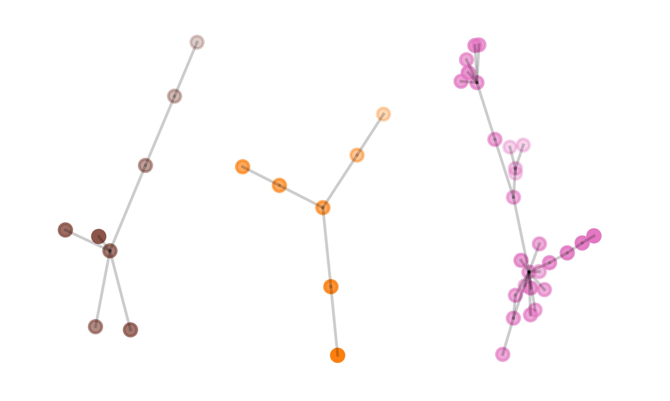
|
| Without user 04 |
\Centerstack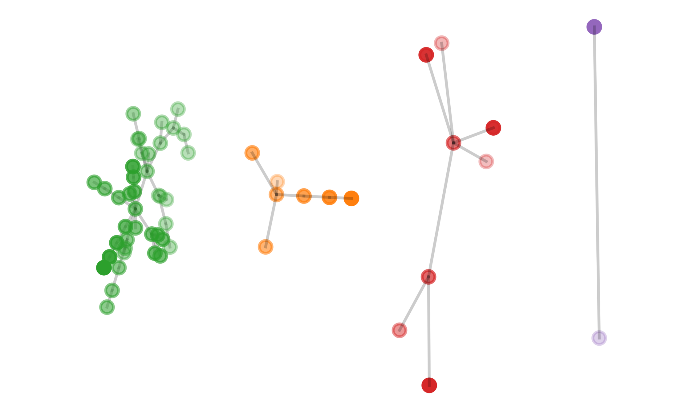
|
\Centerstack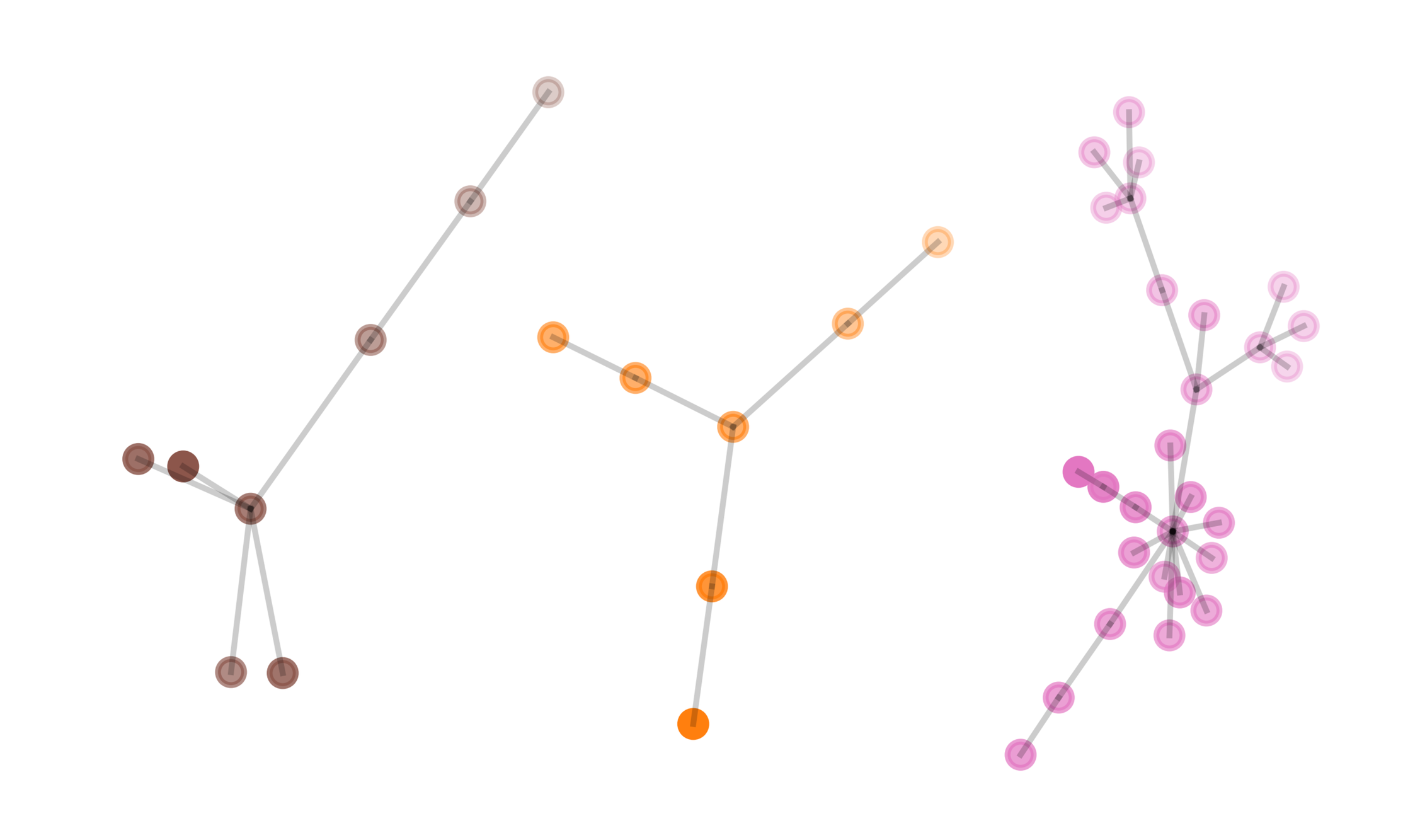
|
| Without user 05 |
\Centerstack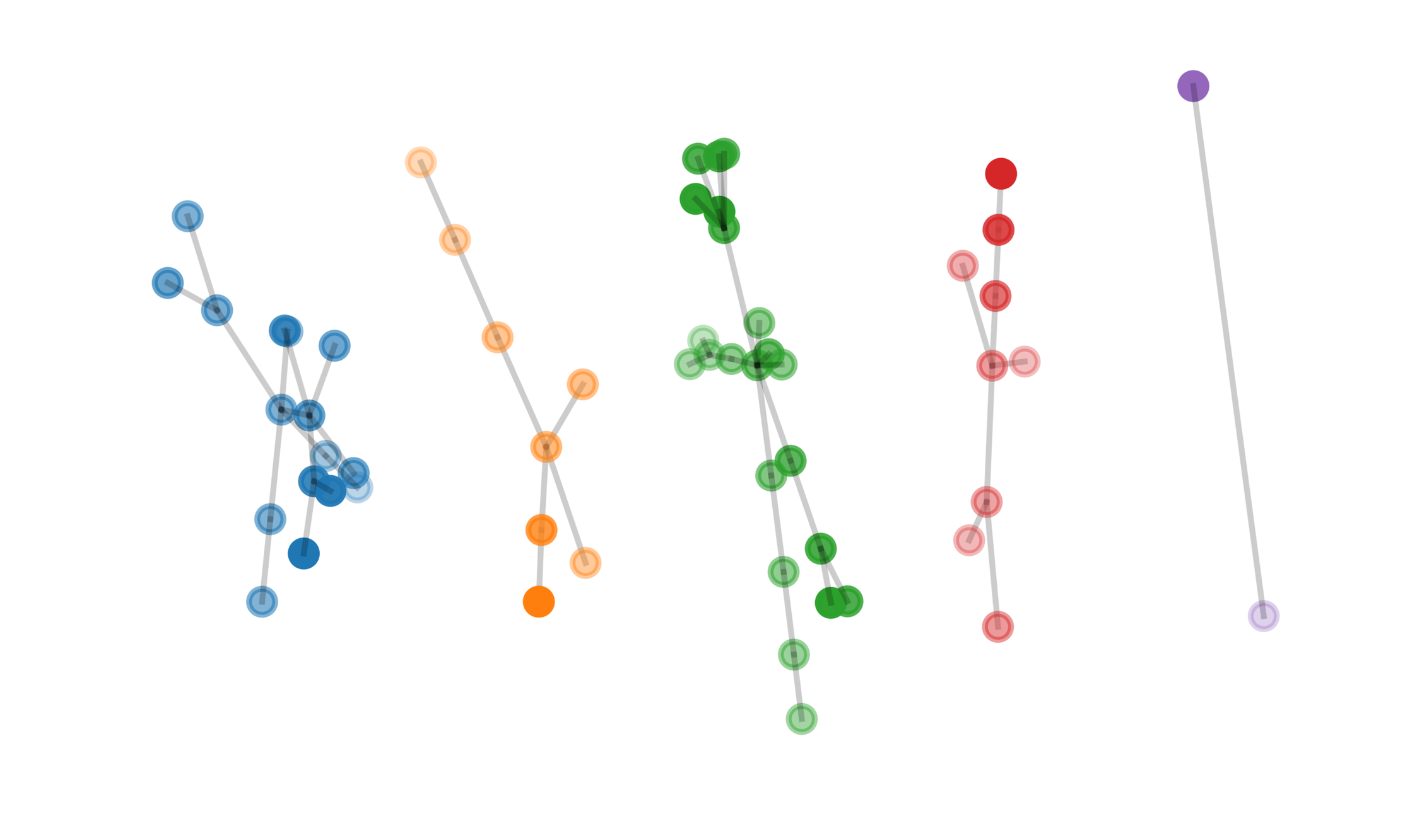
|
\Centerstack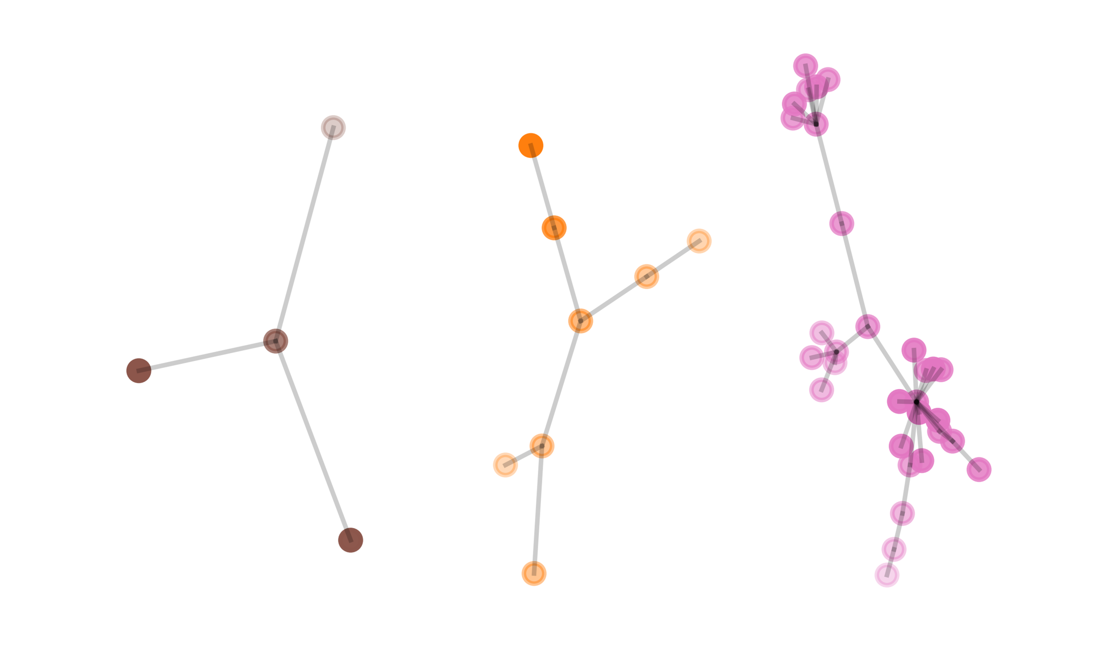
|
| Without user 06 |
\Centerstack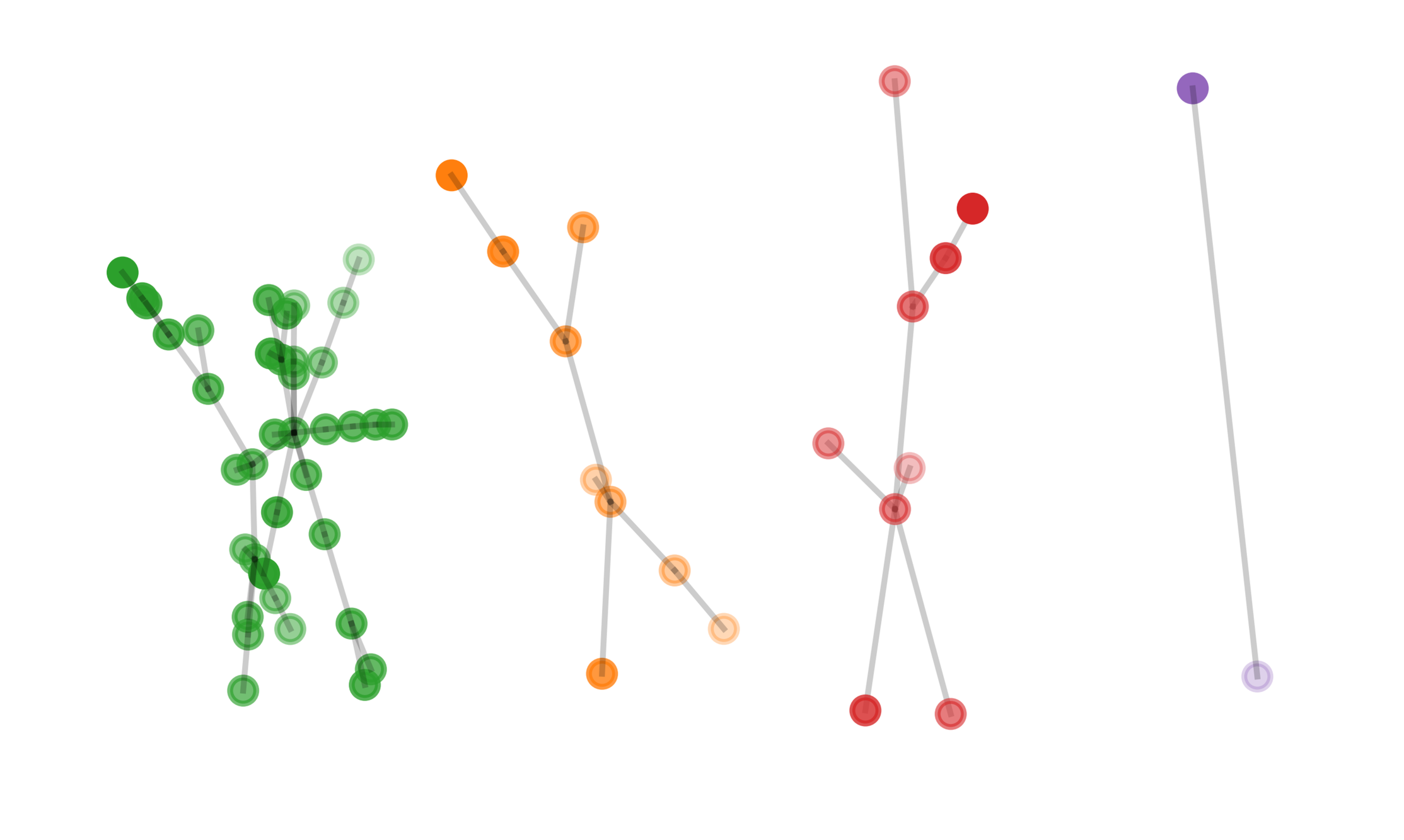
|
\Centerstack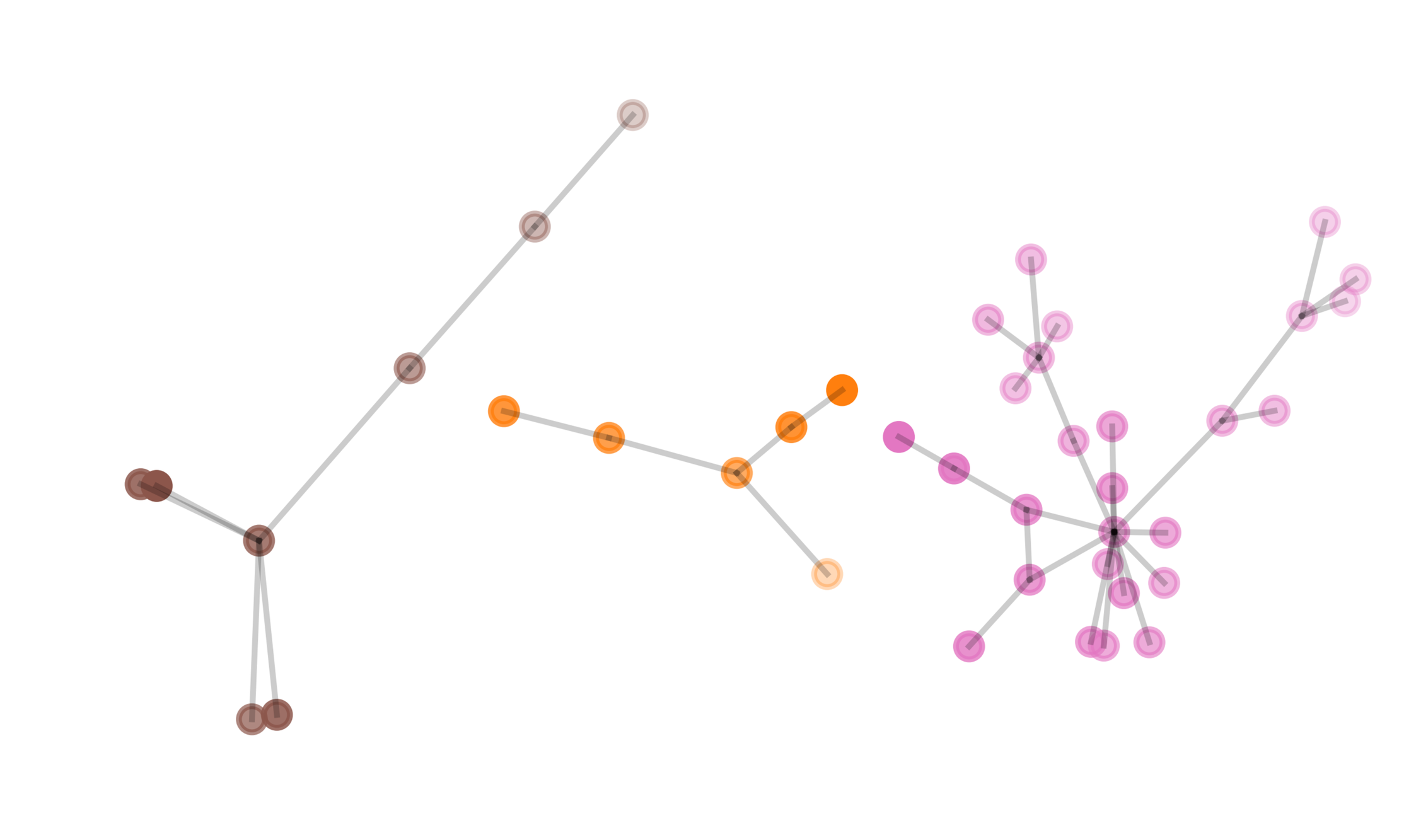
|
| BRM | FRM | |
| Without user 07 |
\Centerstack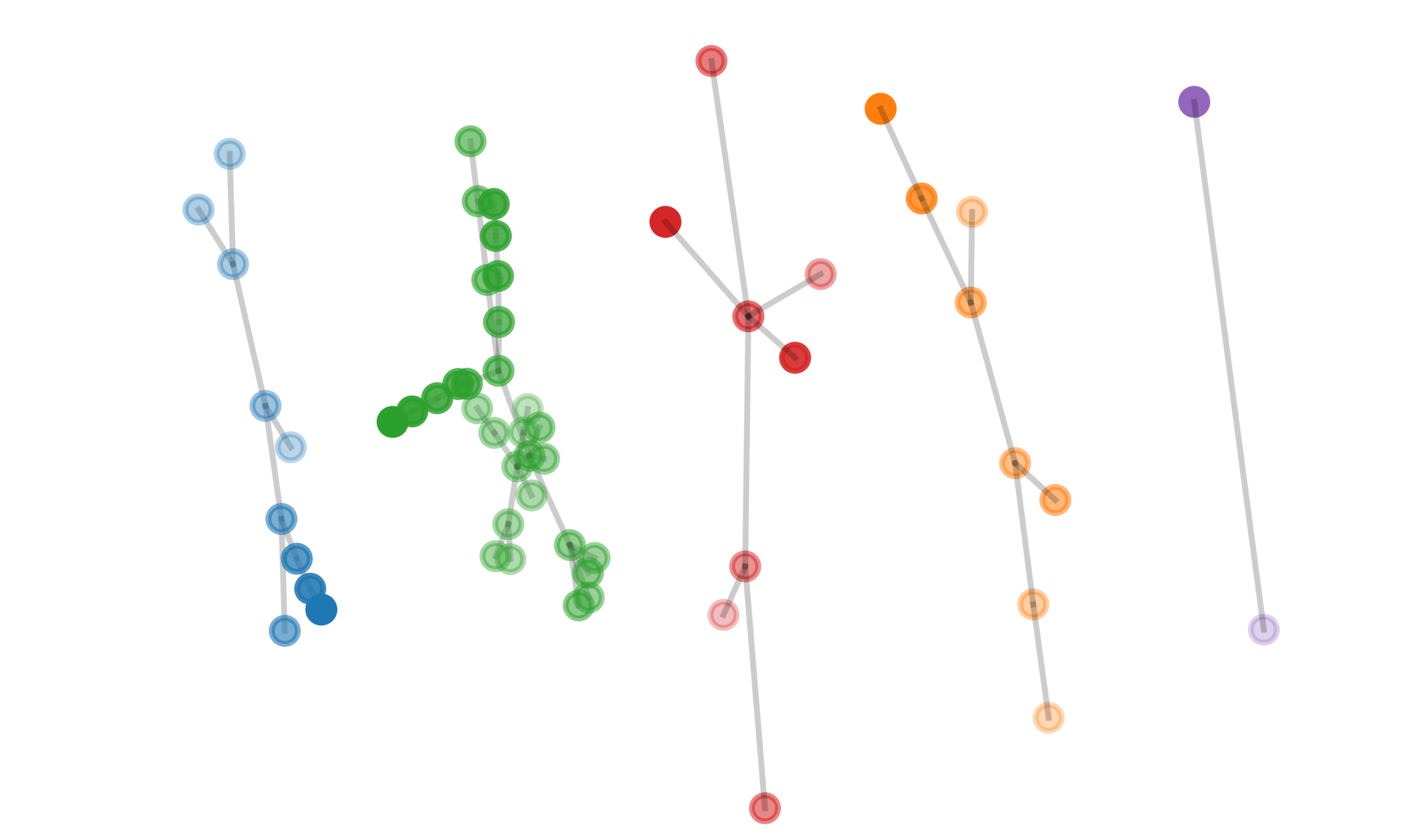
|
\Centerstack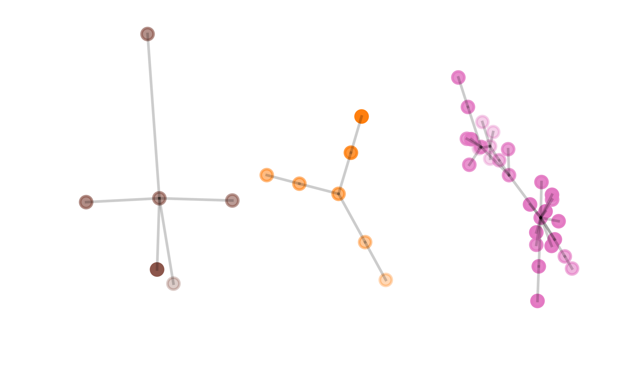
|
| Without user 08 |
\Centerstack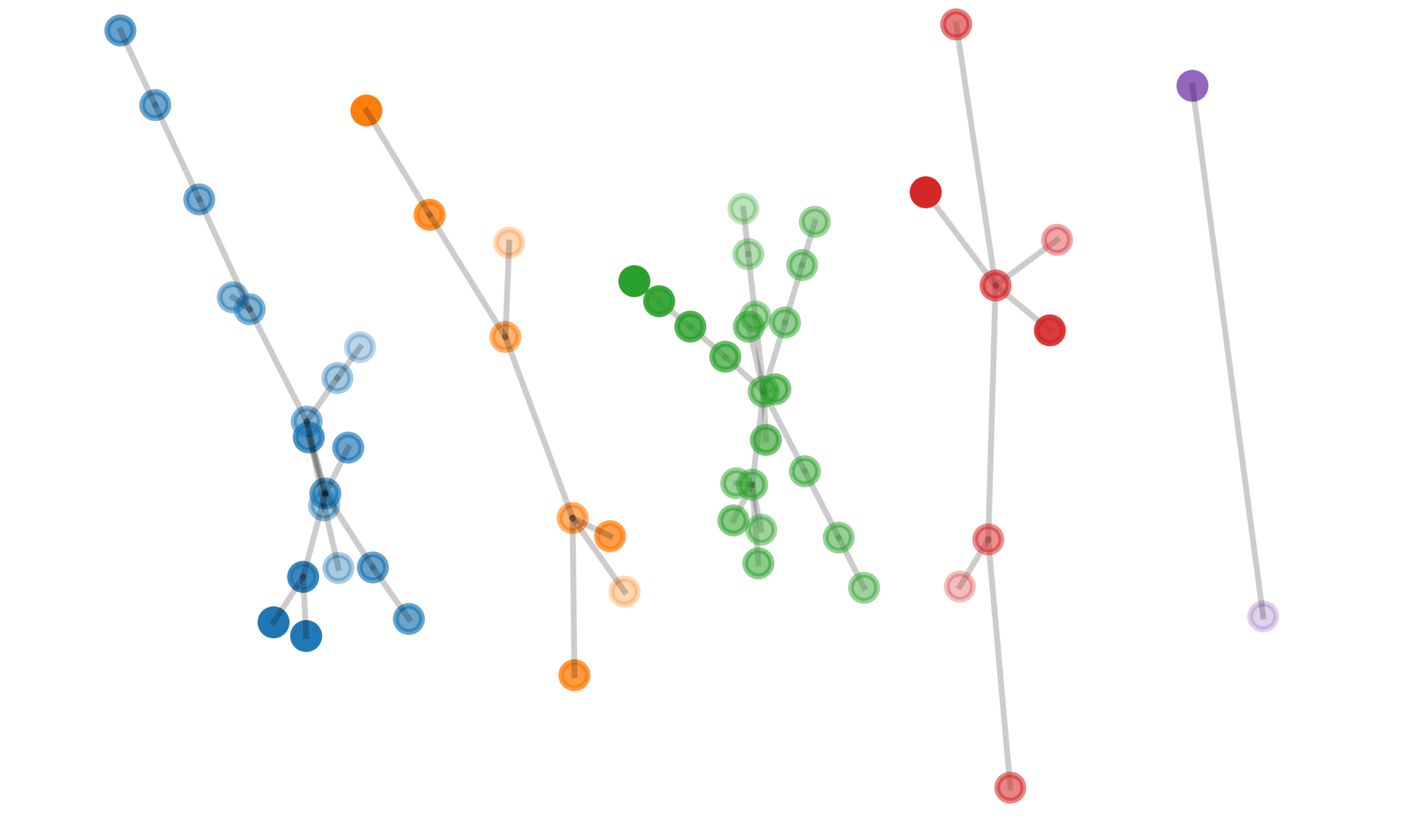
|
\Centerstack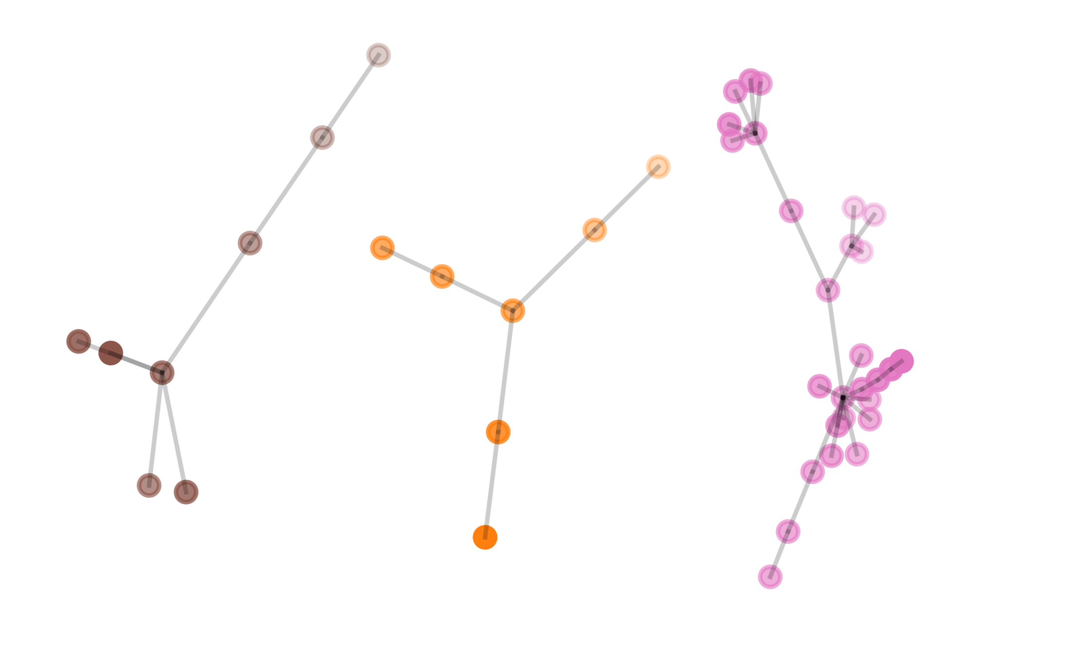
|
| Without user 09 |
\Centerstack
|
\Centerstack
|
| BRM | FRM | |
| Without user 10 |
\Centerstack
|
\Centerstack
|
| Without user 11 |
\Centerstack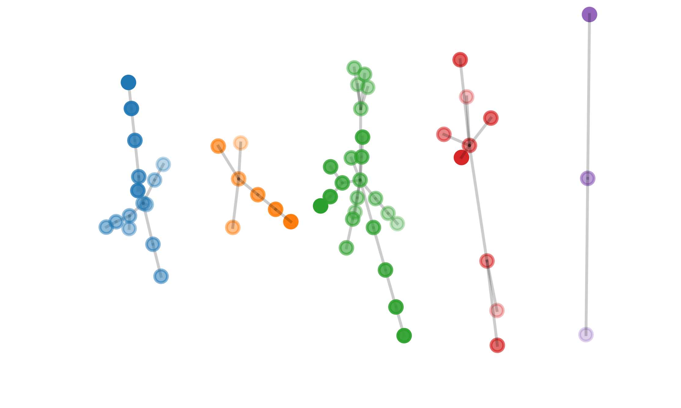
|
\Centerstack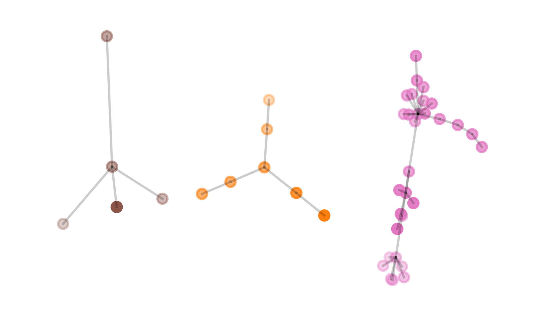
|
| Without user 12 |
\Centerstack
|
\Centerstack
|