[]\acmYear \copyrightyear \acmPrice
Graph Neural Networks for Decentralized Multi-Robot Path Planning
Abstract.
Effective communication is key to successful, decentralized, multi-robot path planning. Yet, it is far from obvious what information is crucial to the task at hand, and how and when it must be shared among robots. To side-step these issues and move beyond hand-crafted heuristics, we propose a combined model that automatically synthesizes local communication and decision-making policies for robots navigating in constrained workspaces. Our architecture is composed of a convolutional neural network (CNN) that extracts adequate features from local observations, and a graph neural network (GNN) that communicates these features among robots. We train the model to imitate an expert algorithm, and use the resulting model online in decentralized planning involving only local communication and local observations. We evaluate our method in simulations by navigating teams of robots to their destinations in 2D cluttered workspaces. We measure the success rates and sum of costs over the planned paths. The results show a performance close to that of our expert algorithm, demonstrating the validity of our approach. In particular, we show our model’s capability to generalize to previously unseen cases (involving larger environments and larger robot teams).
Key words and phrases:
Multi-Agent Path Finding; Decentralized Planning; Deep Learning; Graph Neural Networks;(Emails: ql295, asp45@cam.ac.uk)
1. Introduction
Efficient and collision-free navigation in multi-robot systems is fundamental to advancing mobility. The problem, generally referred to as Multi-Robot Path Planning (MRPP) or Multi-Agent Path Finding (MAPF), aims at generating collision-free paths leading robots from their origins to designated destinations. Current approaches can be classified as either coupled or decoupled, depending on the structure of the state space that is searched. While coupled approaches are able to ensure the optimality and completeness of the solution, they involve centralized components, and tend to scale poorly with the number of robots Silver (2005); Standley and Korf (2011). Decoupled approaches, on the other hand, compute trajectories for each robot separately, and re-plan only in case of conflicts Van den Berg et al. (2008); van den Berg and Overmars (2005); Wu et al. (2020). This can significantly reduce the computational complexity of the planning task, but generally produces sub-optimal and incomplete solutions. Balancing optimality and completeness with the complexity of computing a solution, however, is still an open research problem Barer et al. (2014); Sartoretti et al. (2019).
This work focuses on multi-robot path planning for scenarios where the robots are restricted in observation and communication range, and possess no global reference frame for localization. This naturally arises when considering physical robots equipped with hardware constraints that limit their perception and communication capabilities Matignon et al. (2012). These scenarios impose a decentralized structure, where at any given point in time, robots have only partial information of the system state. In this paper, we propose a combined architecture, where we train a convolutional neural network (CNN) Krizhevsky et al. (2012) that extracts adequate features from local observations, and a graph neural network (GNN) to communicate these features among robots Gama et al. (2019b) with the ultimate goal of learning a decentralized sequential action policy that yields efficient path plans for all robots. The GNN implementation seamlessly adapts to the partial information structure of the problem, since it is computed in a decentralized manner. We train this architecture to imitate an optimal coupled planner with global information that is available offline at training time. Further, we develop a dataset aggregation method that leverages an online expert to resolve hard cases, thus expediting the learning process. The resulting trained model is used online in an efficient, decentralized manner, involving communication only with nearby robots. Furthermore, we show that the model can be deployed on much larger robot teams than the ones it was trained on.
2. Related work and Contribution
Related work. Classical approaches to multi-robot path planning can generally be described as either centralized or decentralized. Centralized approaches are facilitated by a planning unit that monitors all robots’ positions and desired destinations, and returns a coordinated plan of trajectories (or way-points) for all the robots in the system. These plans are communicated to the respective robots, which use them for real-time on-board control of their navigation behavior. Coupled centralized approaches, which consider the joint configuration space of all involved robots, have the advantage of producing optimal and complete plans, yet tend to be computationally very expensive. Indeed, solving for optimality is NP-hard Yu and LaValle (2013), and although significant progress has been made towards alleviating the computational load Sharon et al. (2015); Ferner et al. (2013), these approaches still scale poorly in environments with a high number of potential path conflicts.
Decentralized approaches provide an attractive alternative to centralized approaches, firstly, because they reduce the computational overhead, and secondly, because they relax the dependence on centralized units. This body of work considers the generation of collision-free paths for individual robots that cooperate only with immediate neighbors Desaraju and How (2012); Wu et al. (2020), or with no other robots at all Van den Berg et al. (2008). In the latter case, coordination is reduced to the problem of reciprocally avoiding other robots (and obstacles), and can generally be solved without the use of communication. Yet, by taking purely local objectives into account, global objectives (such as path efficiency) cannot be explicitly optimized. In the former case, it has been shown that monotonic cost reduction of global objectives can be achieved. This feat, however, relies on strong assumptions (e.g., problem convexity and invariance of communication graph Wang et al. (2018); Rotkowitz and Lall (2005)) that can generally not be guaranteed in real robot systems.
Learning-based methods have proven effective at designing robot control policies for an increasing number of tasks Rajeswaran et al. (2017); Tobin et al. (2017). The application of learning-based methods to multi-robot motion planning has attracted particular attention due to their capability of handling high-dimensional joint state-space representations, by offloading the online computational burden to an offline learning procedure. The work in Everett et al. (2018) proposes a decentralized multi-agent collision avoidance algorithm based on deep reinforcement learning. Their results show that significant improvement in the quality of the path (i.e., time to reach the goal) can be achieved with respect to current benchmark algorithms (e.g., ORCA Van den Berg et al. (2008)). Also in recent work, Sartoretti et al. Sartoretti et al. (2019) propose a hybrid learning-based method called PRIMAL for multi-agent path-finding that uses both imitation learning (based on an expert algorithm) and multi-agent reinforcement learning. It is note-worthy that none of the aforementioned learning-based approaches consider inter-robot communication, and thus, do not exploit the scalability benefits of fully decentralized approaches. Learning what, how, and when to communicate is key to this aim.
Of particular interest to us is the capability of learning-based methods to handle high-dimensional joint state-space representations, useful when planning for large-scale collective robotic systems, by offloading the online computational burden to an offline learning procedure Tolstaya et al. (2019); Khan et al. (2020); Everett et al. (2018). The fact that each robot must be able to accumulate information from other robots in its neighborhood is key to this learning procedure. From the point of view of an individual robot, its local decision-making system is incomplete, since other agents’ unobservable states affect future values. The manner in which information is shared is crucial to the system’s performance, yet is not well addressed by current machine learning approaches. Graph Neural Networks (GNNs) promise to overcome this deficiency Scarselli et al. (2009); Gama et al. (2019b). They capture the relational aspect of robot communication and coordination by modeling the collective robot system as a graph: each robot is a node, and edges represent communication links Prorok (2018). Although GNNs have been applied to a number of problem domains, including molecular biology Duvenaud et al. (2015), quantum chemistry Gilmer et al. (2017), and simulation engines Battaglia et al. (2016), they have only very recently been considered within the multi-robot domain, for applications of flocking and formation control Prorok (2018); Tolstaya et al. (2019); Khan et al. (2020).
Contributions. The application of GNNs to the problem of multi-robot path planning is novel. Our particular GNN implementation offers an efficient architecture that operates in a localized manner, whereby information is shared over a multi-hop communication network, through explicit communication with nearby neighbors only Gama et al. (2019b). Our key contribution in this work is the development of a framework that can learn what information needs to be shared between robots, such that each robot can make a decision based on this local information; importantly, our robots only have local, relative information about their positions and goals (i.e., they possess no global reference frame). This framework is composed of a convolutional neural network (CNN) that extracts adequate features from local observations, and a graph neural network (GNN) that learns to explicitly communicate these features among robots. By jointly training these two components, the system is able to best determine what information is relevant for the team as a whole, and share this to facilitate efficient path planning. The proposed model is trained to imitate a centralized coupled planner, and makes use of a novel dataset aggregation method that leverages an online expert to resolve hard cases, thus expediting the learning process. We achieve performance that is close to that of optimal planners in terms of success rate and flowtime (sum of path costs), while also being able to generalize to previously unseen cases, such as larger robot teams and environments.
3. Problem formulation
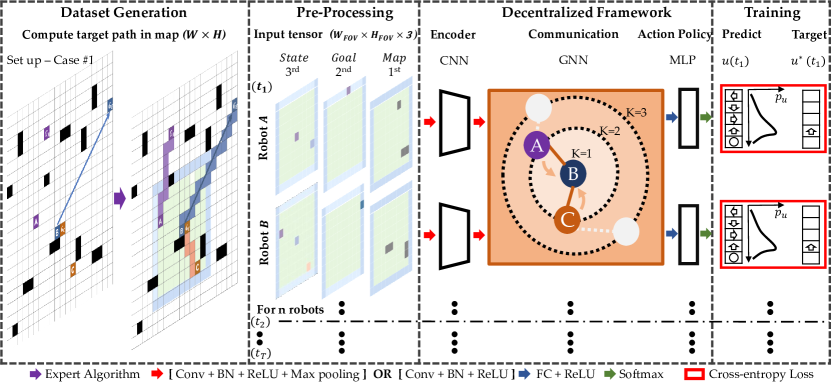
Let be the set of robots. At time , each robot perceives its surroundings within a given field of vision; although the robot knows where its own target destination is located, this information is clipped to the field of vision in a local reference frame (see Fig. 1). Furthermore, we assume no global positioning of the robots. This map perceived by robot is denoted by where and are the width and height, respectively, and are determined by the field of vision radius .
The robots can communicate with each other as determined by the communication network. We can describe this network at time by means of a graph where is the set of robots, is the set of edges and is a function that assigns weights to the edges. Robots and can communicate with each other at time if . The corresponding edge weight can represent the strength of the communication (or be equal to if we are only modeling whether there is a link or not). For instance, two robots and , with positions respectively, can communicate with each other if for a given communication radius . This allows us to define an adjacency matrix representing the communication graph, where if .
In this work, we formulate the multi-agent path planning problem as a sequential decision-making problem that each robot solves at every time instant , with the objective of reaching its destination. More formally, the goal of this work is to learn a mapping that takes the maps and the communication network at time and determines an appropriate action . We want the action to be such that it contributes to the global objective of moving the robots towards their destinations in the shortest possible time while avoiding collisions with other robots and with obstacles that might be present. The objective is to train the network to perform as well as a coupled centralized expert, while restricting robots to partial observations. The mapping has to be restricted to involve communication only among nearby robots, as dictated by the network at each time instant .
4. Graph Neural Networks
In order to guarantee that the mapping is restricted to communications only among nearby robots, we parametrize it by means of a GNN, which is a naturally decentralized solution (Sec. 4.2). We then train this GNN to learn appropriate actions that contribute to the global objective by means of supervised learning through an expert algorithm (i.e., imitation learning) (Sec. 5.5).
4.1. Graph Convolutions
Assume that each robot has access to observations at time . Let be the observation matrix where each row collects these observations at each robot , ,
| (1) |
Note that the columns represent the collection of the observation across all nodes, for . This vector is a graph signal Ortega et al. (2018), since it assigns a scalar value to each node, so that .
To formally describe the communication between neighboring agents, we need a concise way of describing the graph and relating it to the observations . Towards this end, we use the adjacency matrix . We note that other matrix descriptions of the graph, such as the Laplacian matrix or the Markov matrix are possible. We generically call the graph shift operator (GSO) Ortega et al. (2018).
The operation represents a linear combination of neighboring values of the signal due to the sparsity pattern of . More precisely, note that the value at node for observation after operation becomes
| (2) |
where is the set of nodes that are neighbors of . Also, the second equality in (2) holds because for all .
The linear operation is essentially shifting the values of through the nodes, since the application of updates the value at each node by a linear combination of values in the neighborhood. With the shifting operation in place, we can define a graph convolution Gama et al. (2019b) as linear combination of shifted versions of the signal
| (3) |
where is a set of matrices representing the filter coefficients combining different observations. Several noteworthy comments are in order with respect to (3). First, multiplications to the left of need to respect the sparsity of the graph since these multiplications imply combinations across different nodes. Multiplications to the right, on the other hand, can be arbitrary, since they imply linear combination of observations within the same node in a weight sharing scheme. Second, is computed by means of communication exchanges with -hop neighbors, and is actually computing a summary of the information located at the -hop neighborhood. Therefore, the graph convolution is an entirely local operation in the sense that its implementation is naturally distributed. Third, the graph convolution is actually computing the output of a bank of filters where we take as input observations per node and combine them to output observations per node, . There are graph filters involved in (3) each one consisting of filter taps, i.e., the filter can be described by filter taps and these filter taps are collected in the matrix as .
4.2. Graph Neural Networks
A convolutional GNN Gama et al. (2019b) consists of a cascade of layers, each of which applies a graph convolution (3) followed by a pointwise nonlinearity (also known as activation function)
| (4) |
where, in a slight abuse of notation, is applied to each element of the matrix . The input to each layer is a graph signal consisting of observations and the output has observations so that . The input to the first layer is so that and the output of the last layer corresponds to the action to be taken at time , which could be described by a vector of dimension . The GSO to be used in (4) is the one corresponding to the communication network at time , . At each layer we have a bank of filters described by a set of total filter taps .
We note that, in the present framework, we are running one GNN (4) per time instant , where each time step is determined by the moment the action is taken and the communication network changes. This implies that we need to carry out total communications before deciding on an action. Therefore, it is important to keep the GNN shallow (small ) and the filters short (small ).
In summary, we propose to parametrize the mapping between maps and actions by using a GNN (4) acting on observations obtained by applying a CNN to the input maps. We note that, by choosing this parametrization we are obtaining a mapping that is naturally distributed and that is adequately exploiting the network structure of the data.
5. Architecture
The following sections describe the architecture, of which all components are illustrated in Fig. 1.
5.1. Processing Observations
In an environment () with static obstacles, each robot has a local field-of-view (FOV), the radius of which is defined by , beyond which it cannot ‘see’ anything. The robot itself is located at the center of this local observation, and does not know its global position. The data available at robot is a map of size (Fig. 1 illustrates how we implement such partial observations). The input map is fed into a CNN that is run internally on each robot. This results in a vector containing observations (1), . These observations can then be communicated to nearby robots. The intuition behind using a CNN is to process the input map into a higher-level feature tensor describing the observation, goal and states of other robots. This feature tensor is then transmitted via the communication network, as described in the following section,Sec. 5.2.
5.2. Communication
Each individual robot communicates its compressed observation vector with neighboring robots within its communication radius over the multi-hop communication network, whereby the number of executed hops is limited by . As described in Sec. 4.2, we apply our GNN to aggregate and fuse the states within this -hop neighborhood of robots , for each robot . The output of the communication GNN is a hyper-representation of the fused information of the robot itself and its -hop neighbors, which is passed to the action policy, as described in Sec. 5.3. We note that each robot carries a local copy of the GNN, hence resulting in a localized decision-making policy.
5.3. Action Policy
We formulate the path-finding problem as a sequential classification problem, whereby an optimal action is chosen at each time step. We adopt a local multi-layer perceptron (MLP) to train our action policy network. More specifically, each node applies a MLP to the aggregated features resulting from the communication GNN. This MLP is the same across all nodes, resembling a weight-sharing scheme. The action taken by robot is given by a stochastic action policy based on the probability distribution over motion primitives, which in our case consists of five discrete options (up, left, down, right, idle), and are represented by one-hot vectors. The final path is represented by the series of sequential actions.
5.4. Network Architecture
We construct our CNN architecture by using Conv2d-BatchNorm2d-
ReLU-MaxPool2d and Conv2d-BatchNorm2d-ReLU blocks sequentially three times.
All kernels are of size 3 with a stride of 1 and zero-padding. In the GNN architecture, we deploy a single layer GNN (as described in Sec. 4.2) and set as the number of input observations and output observations . Note that we can tune the filter taps for non-communication () and multi-hop communication (). In the action policy, we use a linear soft-max layer to decode the output observations from the GNN with features into the five motion primitives.
5.5. Learning from Expert Data
To train our models, we propose a supervised learning approach based on expert data (i.e., imitation learning). We assume that, at training time, we have access to an optimal trajectory of actions for all the robots, and the corresponding maps obtained for this trajectory , collected in a training set . Then, we train the mapping so that the output is as close as possible to the corresponding optimal action using a cross entropy loss . If the mapping is parametrized in terms of a GNN (4) then this optimization problem becomes
| (5) |
We are optimizing over the filters in the CNN required to process the map as well as the set of matrices that contains the learnable parameters of the communication GNN. Note that the number of parameters is independent of the size of the network .
Imitation learning rests on the availability of an optimal solution (further elaborated in Sec. 5.6, below). While this solution might be computationally expensive, or even intractable for large networks, we only need it at training time. Once trained, the GNN models can be deployed in different communication topologies Gama et al. (2019a), including those with a larger number of robots as is evidenced in the numerical experiments of Sec. 6.3. Given the decentralized nature of the parametrizations, the trained models are efficient in the sense that their computation is distributed among the agents, demanding only communication exchanges with one-hop neighbors.
5.6. Expert Data Generation
As described in our problem statement in Sec. 3, the robots operate in a grid world of size with static obstacles randomly placed throughout the map. For each grid world, we generate cases randomly, i.e., problem instances, which consist of pairs of start and goal positions for all robots (we also refer to this as a configuration). We filter duplicates or invalid cases, and store the remaining cases in a setup pool, which is randomly shuffled at training time. For each case, we generate the optimal solution. Towards this end, we run an expert algorithm: Conflict-Based Search (CBS) Sharon et al. (2015) (which is a similar approach as taken in Sartoretti et al. (2019)). This expert algorithm computes our ‘ground-truth paths’ (the sequence of actions for individual robots), within a timeout, for a given initial configuration. Our data set comprises cases for any given grid world and number of agents. This data is divided into a training set (), a validation set (), and a testing set ().
5.7. Policy Execution with Collision Shielding
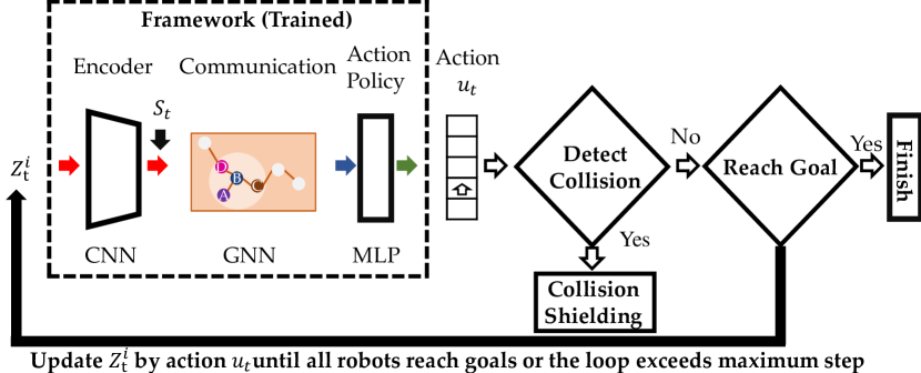
At inference stage, we execute the action policy with a protective mechanism that we name collision shielding. Since it is not guaranteed that robots learn collision-free paths, we require this additional mechanism to guarantee that no collisions take place. Collision shielding is implemented as follows: (i) if the inferred action would result in a collision with another robot or obstacle, then that action is replaced by an idle action; (ii) if the inferred actions of two robots would result in an edge collision (having them swap positions), then those actions are replaced by idle actions. It is entirely possible that robots remain stuck in an idle state until the timeout is reached. When this happens, we count it as a failure case. The overall inference process is summarized in Alg. 1 and Fig. 2.
5.8. Dataset Aggregation during Training
The use of collision shielding leads to failure cases due to potential deadlocks in the actions taken by the robots, where some of them remain stuck in an idle state. To overcome such deadlocks, we propose a dataset aggregation method that makes use of an online expert (OE) algorithm, during training. More specifically, every epochs, we select random cases from the training set and identify which ones are stuck in a deadlock situation. Then, we run the expert starting from the deadlock configuration in order to unlock them into moving towards their goal. The resulting successful trajectory is added to the training set and this extended training set is then used in the following epochs. This process is detailed in Alg. 2. We note that no change is made to the validation or test sets. This dataset aggregation method is similar to the approach in DAgger Ross et al. (2011), but instead of correcting every failed trajectory, we only correct trajectories from a randomly selected pool of cases, as calls to our expert algorithm are time-consuming. Another key difference is that we need to resort to an explicit measure of failure (i.e., through the use of a timeout), since focusing on any deviations from the optimal path (as in the DAgger approach) may be misleading, because those paths may still lead to very competitive solutions in our problem setting.
6. Performance Evaluation
To evaluate the performance of our method, we perform two sets of experiments, (i) on networks trained and tested on the same number of robots, and (ii) on networks trained on a given number of robots, and tested on previously unseen team sizes (both larger and smaller).
6.1. Metrics
1) Success Rate () , is the proportion of successful cases over the total number of tested cases . A case is considered successful (complete) when all robots reach their goal prior to the timeout;
2) Flowtime Increase () , measures the difference between the sum of the executed path lengths () and that of expert (target) path (). We set the length of the predicted path (Alg. 1 and Fig. 2), if the robot does not reach its goal. Here, is the makespan of the solution generated by the expert algorithm.
6.2. Experimental Setup
Our simulations were conducted using a 12-core, 3.2Ghz i7-8700 CPU and an Nvidia GTX 1080Ti GPU with 32 and 11GB of memory, respectively. The proposed network was implemented in PyTorch v1.1.0 Paszke et al. (2017), and was accelerated with Cuda v10.0 APIs. We used the Adam optimizer with momentum . The learning rate scheduled to decay from to within 150 epochs, using cosine annealing. We set the batch size to , and L2 regularization to . The online expert on the GNN is deployed every epochs on randomly selected cases from the training set.
6.3. Results
We instantiate 600 different maps of size , of which 420 are used for training, 90 for validation, and 90 for testing. We generate 50 cases for each map. The obstacle density is set to , corresponding to the proportion of occupied over free space in the environment. We consider a field of view of radius and a communication radius of . At each time step, each robot runs a forwards pass of its local action policy (i.e., the trained network). At the end of each case (i.e., it is either solved or the timeout is reached), we record the length of each robot’s path and the number of robots that reach their goals, to compute performance metrics according to Sec. 6.1.
6.3.1. Effect of Communication on Flowtime and Success Rates
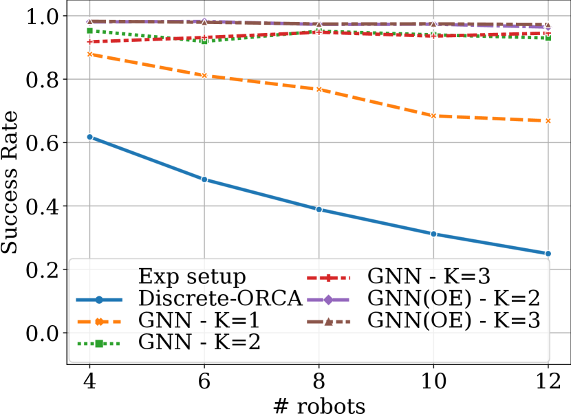
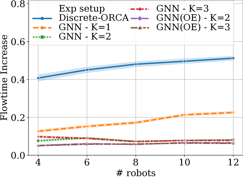
Figures 3(a) and 3(b) show results for the success rate and flowtime increase, respectively, as a function of the number of robots. For each panel, we train a model for , and test it on instances of the same robot team size. In each experiment, we vary the number of communication hops (). Note that for there is no communication involved. Similar to Van den Berg et al. (2008) and Wang et al. (2020), we use a discrete version of a velocity-based collision-avoidance method (Discrete-ORCA) as an additional benchmark against which to test our method.
In both figures, we see a drop in performance for larger teams, but this drop is much more pronounced for the non-communicative GNN (). Our framework generally outperforms the Discrete-ORCA in terms of success rate and flowtime increase.
6.3.2. Generalization
Fig. 4(a) and 4(b) summarize the generalization capability of our model for success rate and flowtime increase, respectively. The experiment was carried out by testing networks across previously unseen cases. The tables specify the number of robots trained on in the rows, and the number of robots tested on in the columns. The results demonstrate strong generalization capabilities.


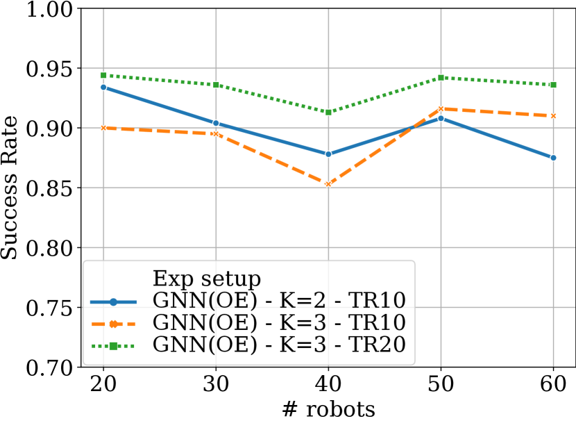
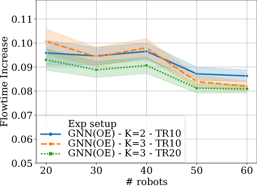
We perform subsequent experiments on larger robot teams to further test the generalization. Results in Fig. 5 show that our network, trained on only 10 robots scales to teams of sixfold size. We test the network in different grid map, where the map sizes are scaled to preserve the effective robot density. Notably, the results show no degradation of performance.
We train the GNN () with and without the online expert (OE) implementation on 10 robots, and test it on 60 robots in environments, respectively. The grid maps are scaled to preserve the same effective density , where the number of obstacles , is the obstacle density in the map () and is the number of robots.
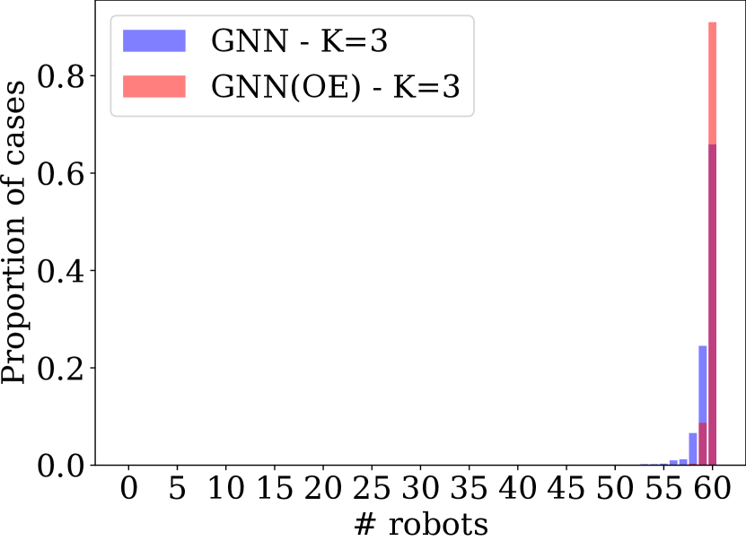
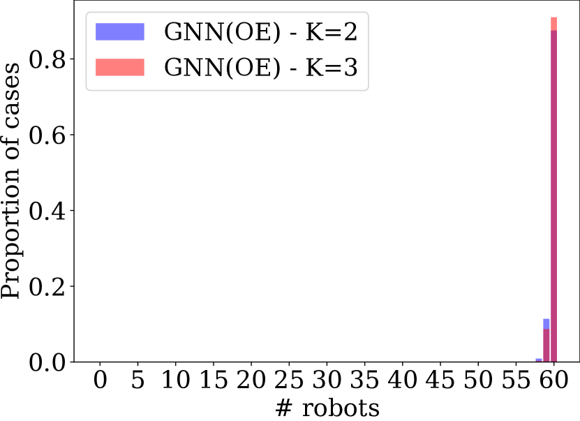
Different from our success rate metric, which only considers complete cases (all robots reach their goals), Fig. 6 presents the proportion of cases distributed over the number of robots reaching their goals. The distributions show that more than 75% of all robots always reach their goals across all implementations. In 97% of cases, more than 95% of robots (57 out of 60) reach their goals. For instance, there are 995 out of 1000 cases (99.5%), where at least 54 robots reach their goals with the GNN () without OE implementation (worst implementation). We see from Fig. 6(a) how the GNN network with OE tends to generalize better than the GNN without OE, since the proportion of robots reaching the goal is larger. In Fig. 6(b), we see how an increased communication hop count (from to ) contributes to a slightly larger proportion of robots reaching their goals.
7. Discussion and Future Work
Our results show that the decentralized framework generalizes to different numbers of robots, as seen in Sec. 6.3.1 and Sec. 6.3.2. We note that a single forward pass of our model (enabling a robot to predict its action) takes only on the workstation described in Sec. 6.2. In addition to the decentralized nature of our solution, this speed of computation is beneficial in real-world deployments, where each robot runs its own (localized) action policy. In contrast, the expert algorithm Sharon et al. (2015) is intractable for more than 14 agents in dense environments within the given timeout; this is corroborated by results in Barer et al. (2014); Sartoretti et al. (2019).
The experiments in in Sec. 6.3.2 showed the capability of our decentralized policy to generalize to robot teams across different sizes. Fig. 4(a) and Fig. 4(b) showed that the framework trained in smaller robot teams () tends to perform worse than those trained in larger teams (), across any unseen instances (larger as well as smaller in size). The intuition for the cause of this phenomenon can be due to two main factors. Firstly, larger robot teams tend to cause more collisions, allowing the policy to learn how to plan more efficient paths more quickly. Secondly, policies trained on very small robot teams (e.g. 4 robots), tend to produce communication topologies that are idiosyncratic, and hence, may generalize more poorly. Results in Fig. 5 showed very strong generalization capabilities, with tests scaling to a factor of 6x of the instances trained on, without noticeable performance deterioration.
We also demonstrated that the use of our online expert leads to significant improvements (as seen in Fig. 3). Fig. 6(a) shows how the GNN with the online expert was able to increase the success rate of all 60 robots reaching goal given a framework trained on 10 robots, and contribute to a right-shift of the distribution.
There are some assumptions and corresponding limitations in the current implementation, which will be improved in future work. Firstly, we assumed that communication between robots was achieved instantly without delay. Time-delayed aggregation GNNs Tolstaya et al. (2019) can be introduced to extend our framework to handle time-delayed scenarios. Secondly, inter-robot live-locks and position swaps remain a challenge impeding 100% success. One potential solution to this is to deploy a policy gradient to add a penalty on the action causing such scenarios. Such a strategy (e.g., as implemented in Sartoretti et al. (2019)) is harder to train, and is left for future work.
8. Conclusions
We considered the problem of collision-free navigation in multi-robot systems where the robots are restricted in observation and communication range, and possess no global reference frame for localization. We proposed a combined architecture, composed of a convolutional neural network that extracts adequate features from local observations, and a graph neural network that communicates these features among robots. The key idea behind our approach is that we jointly trained these two components, enabling the system to best determine what information is relevant for the team of robots as a whole. This approach was complemented by a data aggregation strategy that facilitated the learning process.
This work is the first to apply GNNs to the problem of multi-robot path planning. Our results show that we are very close to achieving the same performance as first-principles-based methods; in particular, we showed our model’s capability to generalize to previously unseen cases involving much larger robot teams. Of particular importance is the fact that we can already scale our system to sizes that are intractable for coupled centralized solvers, while remaining computationally feasible through our decentralized approach.
9. Acknowledgments
We gratefully acknowledge the support of ARL grant DCIST CRA W911NF-17-2-0181. A. Prorok was supported by the Engineering and Physical Sciences Research Council (grant EP/S015493/1). We gratefully acknowledge their support. We also thank Binyu Wang and Zhe Liu for their help in providing benchmark algorithms. We thank Alexandre Raymond, Hehui Zheng, Nicholas Timmons, Rupert Mitchell and Weizhe Lin for the helpful discussion. Finally, we would like to thank the anonymous reviewers for the constructive feedback and help in improving this manuscript.
References
- (1)
- Barer et al. (2014) Max Barer, Guni Sharon, Roni Stern, and Ariel Felner. 2014. Suboptimal Variants of the Conflict-Based Search Algorithm for the Multi-Agent Pathfinding Problem. In European Conference on Artificial Intelligence. 961–962.
- Battaglia et al. (2016) Peter Battaglia, Razvan Pascanu, Matthew Lai, Danilo Jimenez Rezende, and others. 2016. Interaction networks for learning about objects, relations and physics. In Advances in Neural Information Processing Systems. 4502–4510.
- Desaraju and How (2012) Vishnu R Desaraju and Jonathan P How. 2012. Decentralized path planning for multi-agent teams with complex constraints. Autonomous Robots 32, 4 (2012), 385–403.
- Duvenaud et al. (2015) David K Duvenaud, Dougal Maclaurin, Jorge Iparraguirre, Rafael Bombarell, Timothy Hirzel, Alán Aspuru-Guzik, and Ryan P Adams. 2015. Convolutional networks on graphs for learning molecular fingerprints. In Advances in Neural Information Processing Systems. 2224–2232.
- Everett et al. (2018) M. Everett, Y. F. Chen, and J. P. How. 2018. Motion planning among dynamic, decision-making agents with deep reinforcement learning. In IEEE/RSJ International Conference on Intelligent Robots and Systems. 3052–3059. https://doi.org/10.1109/IROS.2018.8593871
- Ferner et al. (2013) Cornelia Ferner, Glenn Wagner, and Howie Choset. 2013. ODrM*: Optimal multirobot path planning in low dimensional search spaces. In IEEE International Conference on Robotics and Automation. 3854–3859.
- Gama et al. (2019a) F. Gama, J. Bruna, and A. Ribeiro. 2019a. Stability Properties of Graph Neural Networks. arXiv:1905.04497v2 [cs.LG] (4 Sep. 2019).
- Gama et al. (2019b) F. Gama, A. G. Marques, G. Leus, and A. Ribeiro. 2019b. Convolutional Neural Network Architectures for Signals Supported on Graphs. IEEE Trans. Signal Process. 67, 4 (Feb. 2019), 1034–1049.
- Gilmer et al. (2017) Justin Gilmer, Samuel S Schoenholz, Patrick F Riley, Oriol Vinyals, and George E Dahl. 2017. Neural message passing for quantum chemistry. International Conference on Machine Learning 70 (2017).
- Khan et al. (2020) Arbaaz Khan, Ekaterina Tolstaya, Alejandro Ribeiro, and Vijay Kumar. 2020. Graph policy gradients for large scale robot control. In Conference on Robot Learning. 823–834.
- Krizhevsky et al. (2012) Alex Krizhevsky, Ilya Sutskever, and Geoffrey E Hinton. 2012. Imagenet classification with deep convolutional neural networks. In Advances in Neural Information Processing Systems. 1097–1105.
- Matignon et al. (2012) Laëtitia Matignon, Laurent Jeanpierre, and Abdel-Illah Mouaddib. 2012. Coordinated multi-robot exploration under communication constraints using decentralized markov decision processes. In AAAI Conference on Artificial Intelligence.
- Ortega et al. (2018) A. Ortega, P. Frossard, J. Kovačević, J. M. F. Moura, and P. Vandergheynst. 2018. Graph Signal Processing: Overview, Challenges and Applications. Proc. IEEE 106, 5 (May 2018), 808–828.
- Paszke et al. (2017) Adam Paszke, Sam Gross, Soumith Chintala, Gregory Chanan, Edward Yang, Zachary DeVito, Zeming Lin, Alban Desmaison, Luca Antiga, and Adam Lerer. 2017. Automatic Differentiation in PyTorch, In NIPS Autodiff Workshop. Advances in Neural Information Processing Systems, 1–4.
- Prorok (2018) Amanda Prorok. 2018. Graph Neural Networks for Learning Robot Team Coordination. Federated AI for Robotics Workshop, IJCAI-ECAI/ICML/AAMAS 2018; arXiv:1805.03737 [cs] (May 2018). arXiv: 1805.03737.
- Rajeswaran et al. (2017) Aravind Rajeswaran, Kendall Lowrey, Emanuel Todorov, and Sham Kakade. 2017. Towards Generalization and Simplicity in Continuous Control. In Advances in Neural Information Processing Systems. Curran Associates Inc., Red Hook, NY, USA, 6553–6564.
- Ross et al. (2011) Stéphane Ross, Geoffrey Gordon, and Drew Bagnell. 2011. A reduction of imitation learning and structured prediction to no-regret online learning. In International Conference on Artificial Intelligence and Statistics. Fort Lauderdale, FL, USA, 627–635.
- Rotkowitz and Lall (2005) M. Rotkowitz and S. Lall. 2005. A characterization of convex problems in decentralized control. IEEE Trans. Automat. Control 50, 12 (Dec. 2005), 1984–1996. https://doi.org/10.1109/TAC.2005.860365
- Sartoretti et al. (2019) Guillaume Sartoretti, Justin Kerr, Yunfei Shi, Glenn Wagner, TK Kumar, Sven Koenig, and Howie Choset. 2019. PRIMAL: Pathfinding via Reinforcement and Imitation Multi-Agent Learning. IEEE Robotics and Automation Letters 4 (2019), 2378–2385. Issue 3.
- Scarselli et al. (2009) Franco Scarselli, Marco Gori, Ah Chung Tsoi, Markus Hagenbuchner, and Gabriele Monfardini. 2009. The graph neural network model. IEEE Transactions on Neural Networks 20, 1 (2009), 61–80.
- Sharon et al. (2015) Guni Sharon, Roni Stern, Ariel Felner, and Nathan R Sturtevant. 2015. Conflict-based search for optimal multi-agent pathfinding. Artificial Intelligence 219 (2015), 40–66.
- Silver (2005) David Silver. 2005. Cooperative Pathfinding. In AAAI Conference on Artificial Intelligence and Interactive Digital Entertainment. 117–122.
- Standley and Korf (2011) Trevor Standley and Richard Korf. 2011. Complete Algorithms for Cooperative Pathfinding Problems. In International Joint Conference on Artificial Intelligence. AAAI Press, Barcelona, Catalonia, Spain, Article 1, 6 pages. https://doi.org/10.5591/978-1-57735-516-8/IJCAI11-118
- Tobin et al. (2017) J. Tobin, R. Fong, A. Ray, J. Schneider, W. Zaremba, and P. Abbeel. 2017. Domain randomization for transferring deep neural networks from simulation to the real world. In IEEE/RSJ International Conference on Intelligent Robots and Systems. 23–30. https://doi.org/10.1109/IROS.2017.8202133
- Tolstaya et al. (2019) E. Tolstaya, F. Gama, J. Paulos, G. Pappas, V. Kumar, and A. Ribeiro. 2019. Learning Decentralized Controllers for Robot Swarms with Graph Neural Networks. In Conference Robot Learning 2019. Int. Found. Robotics Res., Osaka, Japan.
- Van den Berg et al. (2008) Jur Van den Berg, Ming Lin, and Dinesh Manocha. 2008. Reciprocal velocity obstacles for real-time multi-agent navigation. In IEEE International Conference on Robotics and Automation. IEEE, 1928–1935.
- van den Berg and Overmars (2005) J. P. van den Berg and M. H. Overmars. 2005. Prioritized motion planning for multiple robots. In IEEE/RSJ International Conference on Intelligent Robots and Systems. IEEE, Edmonton, Alta., Canada, 430–435. https://doi.org/10.1109/IROS.2005.1545306
- Wang et al. (2020) Binyu Wang, Zhe Liu, Qingbiao Li, and Amanda Prorok. 2020. Mobile Robot Path Planning in Dynamic Environments through Globally Guided Reinforcement Learning. arXiv preprint arXiv:2005.05420 (2020).
- Wang et al. (2018) Y. Wang, N. Matni, and J. C. Doyle. 2018. Separable and Localized System-Level Synthesis for Large-Scale Systems. IEEE Trans. Automat. Control 63, 12 (Dec. 2018), 4234–4249. https://doi.org/10.1109/TAC.2018.2819246
- Wu et al. (2020) Wenying Wu, Subhrajit Bhattacharya, and Amanda Prorok. 2020. Multi-Robot Path Deconfliction through Prioritization by Path Prospects. IEEE International Conference on Robotics and Automation (2020). arXiv: 1908.02361.
- Yu and LaValle (2013) Jingjin Yu and Steven M. LaValle. 2013. Structure and Intractability of Optimal Multi-Robot Path Planning on Graphs. In AAAI Conference on Artificial Intelligence. AAAI Press, 1443–1449.