Feasibility of the ion-trap simulation of a class of non-equilibrium phase transitions

Abstract

Our work analyzes the potential of ion traps for the experimental simulation of non-equilibrium phase transitions observed in certain spin-chain models which can be mapped to free-fermion systems. In order to make the dynamics more accessible to an experimenter, we first consider relatively small systems, with few particles. We analyze phase transitions in the non-equilibrium asymptotic regimes of an XY spin chain with a transverse magnetic field and coupled to Markovian baths at the end sites. We study a static open system and a case when the spin chain is periodically kicked. Notably, in the latter case for some anisotropy parameters the dependence on the system size converges rapidly to the many-particle limit, thus facilitating the experimental observation of the dynamics. We also define local observables that indicate the presence of the quantum phase transitions of interest, and we study the effects of the long-range character of the typical interactions obtained in ion traps.

I Introduction

The analysis of non-equilibrium quantum phase transitions is a very active area of research (see, for example, Znidaric_2010 ; Zoller2011 ; Banchi_2014 ; Heyl_2013 ; Vosk_2014 ; Mazza_2012 ). The inclusion of driving elements, non-thermal baths, and/or baths at different temperatures leads to rich phenomena going beyond the traditional quantum phase transitions (QPTs), that is, transitions observed in quantum systems at zero temperature and which take place as a consequence of quantum rather than thermal fluctuations Sachdev . The field of non-equilibrium QPTs has seen in the last decades a huge progress in the possibilities of implementation of the dynamics in the setting of controllable quantum systems provided by ultracold atoms Diehl_2010 ; Baumann_2010 , trapped ions Jurcevic_2017 ; Genway_2014 , NMR Alvarez_2006 , or cavity QED Morrison_2008 to name a few.

A recent series of articles shows the presence of non-equilibrium phase-transitions in a particular model of driven XY spin chains, which can be mapped to quadratic open fermionic systems Prosen2008 ; Prosen2010 ; Prosen2011 . In this work we provide an analysis of the feasibility of the implementation of this kind of dynamics in a system of trapped ions. This implies the study of several key aspects: in the first place, one must translate the elements of the original proposal in terms of the dynamics of trapped ions. In this respect, the area of quantum simulations in ion traps is very advanced and our proposal benefits from the resources already available in the literature. We do not elaborate on this aspect since the tools to simulate spin systems with ions are standard and described in detail elsewhere Porras_2004 ; Blatt_2012 .

More importantly, it is necessary to identify the essential signatures of the phase transitions that are still visible in chains with reduced numbers of particles; even though some research groups have been able to perform quantum simulations with large numbers of particles Zhang_2017 ; Britton_2012 , most trapped-ion labs are able to manipulate short chains only. Another difficulty is the fact that the original models studied in Prosen2008 ; Prosen2010 ; Prosen2011 contain only nearest-neighbour interactions, which is essential for the mapping of the spin system to a fermionic model admitting an efficient analytical treatment. However, such short-ranged interactions are very challenging for an experimenter. We thus focus on power-law interactions, which are standard in ion traps but give rise to spin models whose dynamics are harder to calculate. Finally, it is important to define measurable quantities that allow one to observe the phenomena of interest with a moderate number of resources and in moderate time; again, the original models focus on observables that greatly simplify the theoretical calculation but which are not straightforward to measure in an actual implementation because of their non-local character.

This work is organized as follows: In Section II we shortly review the theoretical models of interest. Section III describes the results obtained in the original models when the numbers of chain sites are relatively small, and discusses the convergence to the many-particle limit. Section IV analyzes modifications of the model in order to make it closer to realistic experimental situations: firstly, by changing the observable of interest in order to make it more easily accessible to measurements, and secondly, by considering the effect of long-range correlations. Finally, in Section V we summarize our results. Further details are provided in three appendices.

II The model of interest: an out-of-equilibrium spin chain

The starting point of our work is provided by two articles by Prosen and co-authors Prosen2008 ; Prosen2011 . In the first paper, a problem of an open and out-of-equilibrium spin chain is presented which admits an exact solution of the non-equilibrium steady state using quantization in the space of operators (see the Appendix A and Prosen2008 ). For the steady state found, a quantum phase transition is detected by studying long-range correlations. In the second work, a similar analysis is carried out in presence of a time-dependent periodic driving Prosen2011 . The authors found complex phase diagrams displaying phases of long range and exponentially decaying spin-spin correlations depending on the parameter values chosen. For the periodically kicked chain, the structure of this phase diagram was related with the stationary points of the Floquet quasiparticle dispersion relation.

The first model was the time-independent XY chain of $N$ spins $1/2$ with transverse field, with Hamiltonian Lieb_1961 ; Pfeuty_1970 :

$$H_{\text{t-i}}=\sum_{m=1}^{N-1}\left(\frac{1+\gamma}{2}\sigma_{m}^{x}\sigma_{m+1}^{x}+\frac{1-\gamma}{2}\sigma_{m}^{y}\sigma_{m+1}^{y}\right)+h\sum_{m=1}^{N}\sigma_{m}^{z},$$ (1)

where $\gamma$ is the anisotropy parameter, $h$ is the magnetic field, and for simplicity we set $\hbar=1$. The system is coupled to a pair of Lindblad baths at its ends, with four Lindblad operators $L_{1,2}=\sqrt{\Gamma_{1,2}^{L}}\sigma_{1}^{\pm}$, $L_{3,4}=\sqrt{\Gamma_{1,2}^{R}}\sigma_{N}^{\pm}$, where $\sigma_{j}^{\pm}=(\sigma_{j}^{x}\pm i\sigma_{j}^{y})/2$. The full evolution of the system’s density matrix $\rho$ is thus given by

$$\dot{\rho}=\mathcal{L}\rho=-i[H,\rho]+\sum_{j=1}^{4}2L_{j}\rho L_{j}^{\dagger}-\{L_{j}^{\dagger}L_{j},\rho\}$$ (2)

with the curly brackets denoting the anticommutator. As was shown in Lieb_1961 ; Pfeuty_1970 , the Hamiltonian of the system can be diagonalized by mapping the problem onto a system of free fermions. In the extended model including the coupling with baths at the ends, the Lindblad operators are such that the problem in terms of fermions is still solvable with a similar approach ProsenNJP2008 .

We also consider the periodically kicked XY spin chain governed by the Hamiltonian:

$$H_{\text{t-d}}(t) = H_{0}+H_{1}(t),$$ (3)

$$H_{0} = \sum_{m=1}^{N-1}\left(\frac{1+\gamma}{2}\sigma_{m}^{x}\sigma_{m+1}^{x}+\frac{1-\gamma}{2}\sigma_{m}^{y}\sigma_{m+1}^{y}\right),$$ (4)

$$H_{1} = a\,\delta_{\tau}(t)\sum_{m=1}^{N}\sigma_{m}^{z},$$ (5)

where $\gamma$ is the anisotropy parameter, $\delta_{\tau}(t)=\sum_{m\in\mathbb{Z}}\delta\left(t-m\tau\right)$ is a periodic Dirac function with period $\tau$, and $a=h\tau$ where $h$ is the intensity of the external magnetic field. This system is also coupled to a pair of Lindblad baths at its ends, defined in the same form as in the previous, time-independent model.

In order to solve the problem, the system of $N$ spins is mapped by means of the Wigner-Jordan transformation onto a model with $N$ fermionic particles with creation and annihilation operators $c_{j}^{\dagger},c_{j}$ respectively Lieb_1961 ; Pfeuty_1970 . In this mapping, the spin projection along the $z$ axis in site $j$ is directly related with the presence or absence of a fermionic particle in this site, according to $\sigma_{j}^{z}\equiv 2c_{j}^{\dagger}c_{j}-1$. However, the spin projections along directions $x$ and $y$ are mapped into non-local observables in terms of the fermionic system. Alternatively, instead of working with the $2N$ fermionic creation and annihilation operators, one can use $2N$ Majorana operators $\omega_{j}$ which are given by Hermitean combinations of the former. The mapping between spins and Majorana operators is of the form Prosen2011 :

$$\omega_{2j-1} = \sigma_{j}^{x}\prod_{j^{\prime}<j}\sigma_{j^{\prime}}^{z}\,,$$ (6)

$$\omega_{2j} = \sigma_{j}^{y}\prod_{j^{\prime}<j}\sigma_{j^{\prime}}^{z}\,.$$ (7)

The key observable signaling the transitions in the work by Prosen and collaborators was given by the residual correlation:

$$C_{\rm res}=\frac{\left(\sum_{j,k}^{|j-k|\geq N/2}|C_{j,k}|\right)}{\left(\sum_{j,k}^{|j-k|\geq N/2}1\right)}.$$ (8)

Here, $C_{j,k}$ is the correlation matrix in terms of the Majorana representation of the spin operators Prosen2011 :

$$C_{j,k}={\rm tr}(\omega_{j}\omega_{k}\rho)-\delta_{j,k}\,.$$ (9)

For the case of the kicked model, the correlations in Eq. (8) are evaluated immediately after the kick. With the goal of a possible implementation in mind, it is essential to notice that the correlators $C_{j,k}$ are local in terms of the fermionic model, but highly nonlocal with respect to the original spin operators. This aspect will be analyzed in Section IV.

III Numerical results of the original model in small chains

We now proceed to numerically study the behaviour of this system in cases with few particles. We first consider the case of the time-independent non-equilibrium system and then we move on to analyze the case of the kicked chain. As was reported in Refs. Prosen2008 ; Prosen2011 , for a sufficiently large number $N$ of sites, the main features of the long-range correlation diagrams are no longer affected by the details of the baths at the ends. This is not surprising since the strength of the coupling to the baths is kept constant while the system is taken to the thermodynamic limit; thus, the critical behaviour observed corresponds to the Hamiltonian part of the dynamics. However, the presence of some kind of bath is essential for the analysis since it is necessary in order to have a well-defined asymptotic state. Furthermore, the convergence to this state is fastest when the couplings with the baths are taken to be of the same order of magnitude as the Hamiltonian parameters.

We focus our study on the feasibility of the implementation with small chains for several reasons: first of all, most ion-trap labs in the world can only successfully control small systems. Secondly, the transitions are observed in the asymptotic state, and the rate of convergence to it decreases as the chains get longer. Finally, the number of observables that one needs to measure in order to build the correlation diagram of Prosen and co-authors increases with the number of sites in the chain (for more details see Subsection IV.1). Thus, implementations with relatively long chains become extremely challenging. In the following we show results concerning the behaviour of the different models for an increasing value of $N$; more details are provided in Appendix C.

III.1 Time-independent model

Figure 1: Diagram in the $\gamma-h$ plane showing residual correlator $C_{\rm res}$ plotted in a log-scale with $\Gamma_{1}^{L}=\Gamma_{1}^{R}=0.5$, $\Gamma_{2}^{L}=0.3$, $\Gamma_{2}^{R}=0.1$. The black dashed line shows the function $h=1-\gamma^{2}$ which determines the critical field $h_{c}$. Each panel shows the residual correlation diagram for: (a) $N=5$, (b)  $N=7$, (c)  $N=10$ and (d) $N=17$.

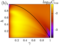
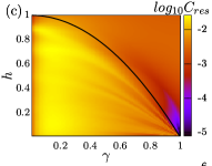
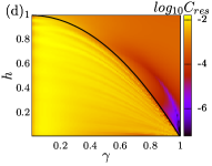
In order to study the feasibility of the experimental implementation of the first model, we analyze the behaviour of the residual correlations (8) as a function of the parameters $\gamma,\,h$ and observe the convergence to the limit $N\gg 1$. As an example, Figure 1 shows the residual correlations for a particular example with $\Gamma_{1}^{L}=\Gamma_{1}^{R}=0.5$, $\Gamma_{2}^{L}=0.3$, $\Gamma_{2}^{R}=0.1$. The different subfigures show cases for different particle numbers, $N=$ 5, 7, 10, and 17, while the black line indicates the phase boundary in the thermodynamic limit. The results show that signatures of the QPT appear for $N\gtrsim 15$. For those values, $C_{\rm res}$ presents an abrupt change which coincides with the theoretical prediction $h_{c}=1-\gamma^{2}$ Prosen2008 .

III.2 Model with periodic kicks

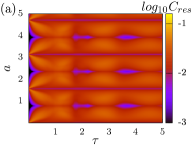
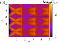
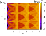
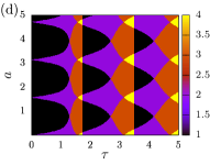
We now perform a similar analysis of the second model, i.e. the open chain with periodic kicks, for different values of the particle number $N$. Figures 2 and 3 show the residual correlation (8) for $\gamma=0.1$ and 0.9 respectively, with subplots (a-c) corresponding to $N=$ 4, 7, 20. We consider the cases $\gamma=0.1$ and $0.9$ as in Prosen2011 , but we prefer to use $a-\tau$ diagrams instead of $h-\tau$ diagrams as in Prosen2011 to display more clearly the periodic dependence of the phase diagram on $a$. This periodicity is related with the time-dependent driving term $\sum_{m}\sigma_{m}^{z}$, which has a period $\frac{\pi}{2}$ and also produces a reflection with respect to the axis $a=\frac{\pi}{4}$. Therefore, one can restrict the analysis to the interval $a\in[0,\frac{\pi}{4})$.

Figure 2: Residual correlator $C_{\rm res}$ in log scale, in the $a-\tau$ plane and with number of sites $N=4$ (a), $N=7$ (b), $N=20$ (c). In panel (d) we show half the total number of non-trivial stationary points of the quasi-particle dispersion relation for kicked XY chain (see Appendix B for details). For all panels we used $\gamma=0.1$ and the same values of the bath terms that were used in the previous figure.

In panel (d) of Figs. 2 and 3, we show half the total number of non-trivial stationary points of the quasi-particle dispersion relation for the infinite kicked XY chain (see Appendix B and Prosen2011 ). The non-equilibrium phase transitions correponding to the sudden appearance of long-range correlations happen at points where the number of stationary points presents jumps. Thus, this quantity was found to determine the shape of the phase diagram Prosen2011 .

In the case with small anisotropy, $\gamma=0.1$, shown in Fig. 2, one can observe that small systems ($N=4$ and 7, in the upper row) already display a structure which resembles that of large chains, with a sharp onset of the long-range correlations forming dark triangles on the left of the diagram. On the contrary, for large anisotropy parameters, $\gamma=0.9$ as in Fig. 3, one has to reach much larger particle numbers ($N\simeq 20$) in order to observe a sudden appearance of long-range correlations at the points where the number of stationary points exhibits a jump (as displayed in subplot d). Besides, for $\gamma=0.1$ the transition that is seen most clearly is the one for the smallest values of $\tau$. From these observations, in the following we focus on the case $\gamma=0.1$ and we restrict to small values of $\tau$.

Figure 3: Residual correlator $C_{\rm res}$ in log scale, in the $a-\tau$ plane and with number of sites $N=4$ (a), $N=7$ (b), $N=20$ (c). In panel (d) we show half the total number of non-trivial stationary points of the quasi-particle dispersion relation for kicked XY chain (see Appendix for details). For all panels we used $\gamma=0.9$ and the same values of the bath terms that were used in the previous figures.

IV Towards a realistic experimental implementation

We have previously shown that the time-independent model for non-equilibrium phase transitions only displays critical behaviour for relatively large chains with $N\gtrsim 15$. On the contrary, the model with periodic kicks and small anisotropy already shows signatures of the phase diagram for very small chains, with $N\gtrsim 5$. For this reason, in the following we will focus only on this second situation. For definiteness, we will take the number of particles fixed at $N=5$.

We consider the possible implementation of the kicked model for non-equilibrium quantum phase transitions using a chain of trapped ions. This setup has been proposed, and used, for spin simulations in several occasions Jurcevic_2017 ; Porras_2004 ; Blatt_2012 ; Monroe_NJP_2011 ; Cormick_2013 ; Jurcevic_2014 . In this context, the internal degrees of freedom of the ions encode the spins, while the Coulomb interaction is used to generate effective spin-spin interactions. In order to achieve this, ions are driven by laser pulses which couple the internal states with the vibrational motion of the ions. If the laser pulses are chosen appropriately, an effective spin-spin interaction is produced Porras_2004 ; Blatt_2012 . We will now discuss how the original model of Prosen and coauthors can be made more experimental-friendly by requiring measurements of local observables, and after this we analyze the effects of the long range of the typical effective interactions achieved in ion-trap simulations of spin models.

IV.1 Local residual correlator

The residual correlation analyzed so far, Eq. (8), is a combination of highly non-local operators in terms of the spin operators (9). The experimentally more accessible quantities are the two-local correlations Monroe_NJP_2011 ; Heyl_2013 ; Blatt_2012 :

$$C_{j,k}^{xx} = \mbox{tr}\left(\sigma_{j}^{x}\sigma_{k}^{x}\rho\right)\,,$$ (10)

$$C_{j,k}^{xy} = \mbox{tr}\left(\sigma_{j}^{x}\sigma_{k}^{y}\rho\right)\,,$$ (11)

$$C_{j,k}^{yy} = \mbox{tr}\left(\sigma_{j}^{y}\sigma_{k}^{y}\rho\right)\,.$$ (12)

From them we define the local residual correlation as:

$$C_{\rm res}^{\rm loc}={\cal P}\left(\sum_{j,k}^{|j-k|\geq N/2}\left(|C_{j,k}^{xx}|+|C_{j,k}^{xy}|+|C_{j,k}^{yy}|\right)\right)$$ (13)

where ${\cal P}$ is the normalization factor given by:

$${\cal P}^{-1}=\sum_{j,k}^{|j-k|\geq N/2}3\,.$$ (14)

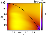
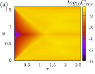
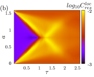
This quantity can be numerically computed from the density matrix corresponding to the asymptotic state. In Fig. 4 we compare local and non-local residual correlations for $\gamma=0.1$. We observe that local residual correlations show the same structure as the correlations which are local in terms of fermionic operators, although with a different intensity (notice the change in the color scale).

We stress that the number of correlations that one needs to measure to obtain $C_{\rm res}^{\rm loc}$ is much smaller than the total number of observables necessary for full state tomography. However, the amount of measurements required to calculate $C_{\rm res}^{\rm loc}$ still scales up as $N^{2}$, which is another reason to prefer simulations that are feasible with small chains. Furthermore, the necessary measurements demand the ability to individually address and rotate the desired spins. This is a non-trivial technical requirement, which also makes the experiment more challenging for longer chains.

Figure 4: Residual correlation as a function of $a$ and $\tau$ in log-scale for $N=5$ in the representative region $a\in(0,\pi/2]$ and with $\gamma=0.1$. Panel (a) shows the residual correlation made of observables which are local in the fermionic space, panel (b) the one made of observables local in the spin space (see main text for details).

IV.2 Long-range interactions in the ion-trap implementation

Previous experiments have implemented the dynamics of effective Ising models with transverse fields, given by

$$H_{\rm Ising}=\hbar\sum_{i<k}^{N}J_{i,k}\sigma_{i}^{x}\sigma_{k}^{x}-\hbar B\sum_{i}^{N}\sigma_{i}^{z},$$ (15)

where $J_{i,k}$ has a dependence on the distance between ions approximately given by a power-law decay $J_{i,k}^{\eta}\propto|j-k|^{-\alpha}$. The sign of the couplings can be chosen by appropriately tuning the lasers Britton_2012 ; Monroe_NJP_2011 , and it has been theoretically shown that the parameter $\alpha$ can be tuned in the range between $\alpha=0$ and $\alpha=3$ Porras_2004 . Experimentally, tuning of $\alpha$ from 0.01 to 2.72 has been demonstrated Britton_2012 . However, interactions in the highest range of values of $\alpha$ are hard to achieve experimentally because the large detunings required lead to low coupling strengths, and thus most experiments have been performed with intermediate values of $\alpha$ Islam_2013 ; Jurcevic_2014 ; Britton_2012 ; Monroe_NJP_2011 .

Thus, we now analyze the simulation of our model of non-equilibrium phase transitions in the kicked spin chain but where the spin-spin interactions are given by the Hamiltonian:

$$H_{\rm exp}=\sum_{j<k}\left(J_{j,k}^{x}\sigma_{j}^{x}\sigma_{k}^{x}+J_{j,k}^{y}\sigma_{j}^{y}\sigma_{k}^{y}\right),$$ (16)

where the matrix elements $J_{j,k}^{\eta}$, with $\eta=x,y$, decay as $J_{j,k}^{\eta}\propto|j-k|^{-\alpha}$. In our system $J_{j,j+1}^{x}=\frac{1+\gamma}{2}$ and $J_{j,j+1}^{y}=\frac{1-\gamma}{2}$. Considering this Hamiltonian and the term associated with the periodic kick we evaluated once more the residual correlations in the asymptotic regime. We note that this is numerically more costly, since in presence of long-term couplings the Jordan-Wigner transformation does not lead to a quadratic fermionic system any more. This means that a compact description of the dynamics is not possible. However, the full computation is still feasible due to the small number of particles.

Figure 5: Local residual correlation maps $a-\tau$ in log-scale for $N=5$ in the representative region $a\in(0,\pi/2]$ and with $\gamma=0.1$. Here we consider the additional terms associated with the long range of the spin-spin interaction. We can observe that the reflection symmetry with respect to the axis $a=\pi/4$ is broken; however, this effect is small and the diagram still shows a sudden appearance of correlations in coincidence with Fig. 4. For panel (a) a power-law decay with $\alpha=3$ was chosen; panel (b) shows the results for the more realistic power $\alpha=2$.

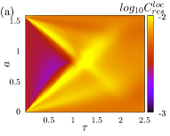
In Fig. 5 we show the results for the local residual correlation $C_{\rm res}^{\rm loc}$ with $\gamma=0.1$ including the power-law decay of interactions, with powers $\alpha=3$ (a) and $\alpha=2$ (b). Both cases are theoretically possible Porras_2004 ; however, case (a), which is closest to the original model, corresponds to a limiting case of infinite laser detuning. Case (b), on the contrary, is within the range which has been experimentally demonstrated Britton_2012 . We observe that the structure of the diagram is similar to the previous Figures, although the new interaction terms affect the reflection symmetry of the correlation with respect to the axis $a=\pi/4$. Clearly, the deformation is much more noticeable for the case $\alpha=2$ which has stronger interactions for distant pairs of sites; this case also shows a lower intensity contrast. Thus, it seems worth pushing the interaction power law to the highest possible values ($\alpha=2.72$ being the fastest decay achieved so far Britton_2012 ); nevertheless, the qualitative features of the diagram are still clearly visible for the case $\alpha=2$.

V Conclusions

We have critically assessed the potential for the ion-trap implementation of the models proposed by Prosen Prosen2008 ; Prosen2011 displaying non-equilibrium quantum phase transitions in spin chains. We analyzed the effects of several key aspects: in the first place, the possibility to observe signatures of the phase transitions in chains with small numbers of particles. There, we observed that the number of sites required depends on the precise model under consideration: for the static model numbers $N\gtrsim 15$ are necessary to identify the position of the critical line, while for the kicked model the number depends strongly on the anisotropy parameter $\gamma$. For $\gamma=0.9$, the shape of the long-range correlation diagram only starts ressembling the right critical structure with relatively large numbers, $N\gtrsim 20$, whereas a small anisotropy $\gamma=0.1$ leads to a diagram displaying the expected onset of long-range correlations with a number of sites $N\gtrsim 5$. In order to make the necessary number of sites as small as possible, we chose to focus on the case $\gamma=0.1$ with small $\tau$.

In a following step, we redefined the original indicator of the presence of long-range correlations in order to make it more experimentally accessible. This meant replacing a quantity which was obtained from local measurements in terms of the fermionic model, and thus nonlocal in the experiment, by one which was defined from observables which are local in terms of the spin operators. We then concluded that the structure of the diagram was still visible when performing this kind of measurement, although the intensity pattern varied with respect to the original results.

Finally, we considered the effect of the presence of long-range interactions in the experimentally feasible ion-trap simulations. We assumed that the effective spin-spin interactions had a power-law decay, and computed the resulting correlation diagrams for powers $\alpha=3$ and $\alpha=2$. While the long-range interactions partially destroyed one of the symmetries of the original model, one could still observe transitions between regimes with and without long-range correlations. We thus conclude that although the exact features of the original article Prosen2011 are not preserved in a realistic implementation, the markers of the transitions are still visible in experimentally achievable conditions.

Appendix A Treatment of Markovian open quasi-free fermionic systems

We review here the formulation used by Prosen for quadratic systems with a bath with linear terms Prosen2010 ; Prosen2011 . The aim of this formulation is to calculate the correlations avoiding the calculation of the density matrix, and it is a generalization of the standard description of Gaussian states by means of the covariance matrix Gaussian . This approach has considerable advantages, leading to a substantial decrease of computational costs in cases when a full analytical solution is not possible. Within this formalism, correlations are obtained by solving a Lyapunov equation, for which there are fast computational solving softwares.

The formulation is performed in terms of the Majorana operators. The authors consider a system of fermions described by $2N$ anticonmmuting Hermitean operators $\omega_{j}$, $j=1,...,2N$, $\{\omega_{j},\omega_{k}\}=2\delta_{j,k}$. One can define Majorana operators in terms of Pauli matrices on $N$ sites as

$$\omega_{2m-1} = \sigma_{m}^{x}\prod_{m^{\prime}<m}\sigma_{m^{\prime}}^{z},$$

$$\omega_{2m} = \sigma_{m}^{y}\prod_{m^{\prime}<m}\sigma_{m^{\prime}}^{z},$$ (17)

The authors consider systems for which both the Hamiltonian ${\cal H}$ and the Lindblad operators $L$ can be simultaneously expressed in terms of a quadratic form and linear forms respectively. In this representation

$${\cal H}=\sum_{j,k}\omega_{j}H_{j,k}\omega_{k}\equiv\underline{\omega}\cdot\mathbb{H}\underline{\omega},$$ (18)

$$L_{\mu}=\sum_{j}\ell_{\mu,j}\omega_{j}\equiv\underline{\ell}_{\mu}\cdot\underline{\omega},$$ (19)

where $\mathbb{H}$ can be chosen to be antisymmetric and imaginary, and $\underline{\ell}_{\mu}\in\mathbb{C}^{2N}$.

The object of interest is the correlation matrix ${\mathbb{C}}$ with elements $C_{j,k}$ defined as:

$$C_{j,k}=\mbox{tr}\left(\omega_{j}\omega_{k}\rho\right)-\delta_{j,k}$$ (20)

If the equations for the evolution of the system do not depend on time, one can obtain the elements of $\mathbb{C}$ in the stationary state through the continuous Lyapunov equation Prosen2010 :

$$\mathbb{XC+CX}^{T}=i\mathbb{Y}\,.$$ (21)

Here, $\mathbb{X}=4\left(i\mathbb{H}+\mathbb{M}_{r}\right)$ and $\mathbb{Y}=4\left(\mathbb{M}_{i}-\mathbb{M}_{i}^{T}\right)$, with the real matrices $\mathbb{M}_{r},~{}\mathbb{M}_{i}$ defined from $\mathbb{M}=\mathbb{M}_{r}+i\mathbb{M}_{i}$, $\mathbb{M}=\sum_{\mu}\underline{\ell}_{\mu}\otimes\overline{\underline{\ell}}_{\mu}$.

On the other hand, when the evolution equations are time-dependent, the covariance matrix $\mathbb{C}$ satisfies

$$\dot{\mathbb{C}}(t)=-\mathbb{X}(t)\mathbb{C}(t)-\mathbb{C}(t)\mathbb{X}^{T}(t)+i\mathbb{Y}(t)$$ (22)

with $\mathbb{X}(t)$ and $\mathbb{Y}(t)$ defined as before but from the time-dependent $\mathbb{H}$ and $\mathbb{M}$. The solution to eq. (22) can be written as Prosen2011

$$\mathbb{C}(t)=\mathbb{Q}(t)\mathbb{C}(0)\mathbb{Q}^{T}(t)-i\mathbb{P}(t)\mathbb{Q}^{T}(t),$$ (23)

where $\mathbb{P}(t)$ and $\mathbb{Q}(t)$ have to fulfill

$$\dot{\mathbb{Q}}(t) = -\mathbb{X}(t)\mathbb{Q}(t),$$ (24)

$$\dot{\mathbb{P}}(t) = -\mathbb{X}(t)\mathbb{P}(t)-\mathbb{Y}(t)[\mathbb{Q}^{T}(t)]^{-1}$$ (25)

with the initial conditions $\mathbb{Q}(0)=\mathbb{I},~{}\mathbb{P}(0)=0$.

In the case studied in Prosen2011 , the temporal dependence of the problem is through a periodic kick in the Hamiltonian, so that ${\cal L}(t+\tau)={\cal L}(t)$, where $\tau$ is the period. The correlation matrix for the stationary state is then obtained solving the discrete Lyapunov equation

$$\mathbb{Q}(\tau)\mathbb{C}_{F}\mathbb{Q}^{T}(\tau)-\mathbb{C}_{F}=i\mathbb{P}(\tau)\mathbb{Q}^{T}(\tau),$$ (26)

where $\mathbb{C}(0)=\mathbb{C}(\tau)=\mathbb{C}_{F}$.

Appendix B Quasi-energy bands of the kicked system

In Ref. Prosen2011 , analyzing the kicked system, it was shown that, when dealing with many particles, the main properties of the residual correlations depend essentially on the Hamiltonian of the bulk. For this reason, the dispersion relation of a kicked XY infinite chain was studied. The system has two quasi-energy bands of the form:

$$\theta_{1,2}(\kappa) = \pm\mbox{arcos}\Big{\{}\cos\left(2\tau h\right)\cos\left[2\tau\varepsilon(\kappa)\right]$$ (27)

$$+\sin\left(2\tau h\right)\sin\left[2\tau\varepsilon(\kappa)\right]\frac{\cos(\kappa)}{\varepsilon(\kappa)}\Big{\}}$$

where $\varepsilon(\kappa)=\sqrt{\cos^{2}(\kappa)+\gamma^{2}\sin^{2}(\kappa)}$ is the quasi-particle energy for the unkicked XY chain, $\kappa\in\left[\left.-\pi,\pi\right.\right)$. As discussed in Refs. Prosen2011 ; Prosen2010 the jumps in the residual correlations $C_{\rm res}$ coincide with jumps in the number of non-trivial stationary points of the quasienergies dispersion relation of the Floquet eigenstates of the system. As the total number of stationary points is always even, the quantity shown in the plots in the main text is half this number.

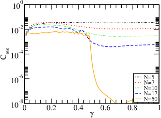
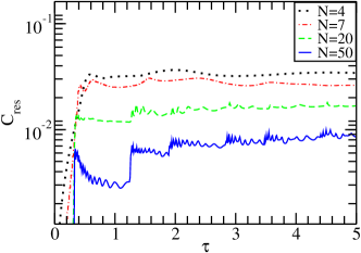
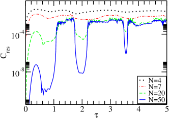
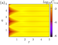
Appendix C Dependence of the residual correlations on the number of sites

In this Appendix we provide further plots showing the behaviour of the residual correlation $C_{\rm res}$, defined in Eq. (8), as the number of sites is increased. In Fig. 6 we plot the residual correlation for different values of $N$. Plot (a) corresponds to the static case as a function of $\gamma$, with $h=0.75$, whereas plots (b) and (c) correspond to the kicked model and show $C_{\rm res}$ as a function of $\tau$, with $a=1.25$, for $\gamma=0.1$ and $0.9$ respectively. One can see that in plots (a) and (c) a number of sites $N$ around 20 is necessary to observe the signatures of the transition. On the contrary, plot (b) indicates that for small anisotropy, $\gamma=0.1$, the transition at smallest $\tau$ is already visible with less than 10 sites.

Figure 6: Residual correlator $C_{\rm res}$ plotted in a log-scale with $\Gamma_{1}^{L}=\Gamma_{1}^{R}=0.5$, $\Gamma_{2}^{L}=0.3$, $\Gamma_{2}^{R}=0.1$, and for different values of $N$. Plot (a) corresponds to the static case as a function of $\gamma$, with $h=0.75$; plots (b) and (c) correspond to the kicked model and show $C_{\rm res}$ as a function of $\tau$, for $\gamma=0.1$ and $0.9$ respectively, and with $a=1.25$.

References

- (1) M. Žnidarič, Exact solution for a diffusive nonequilibrium steady state of an open quantum chain. J. Stat. Mech. L05002 (2010).
- (2) A. Tomadin, S. Diehl and P. Zoller, Nonequilibrium phase diagram of a driven and dissipative many-body system, Phys. Rev. A 83, 013611 (2011).
- (3) Leonardo Banchi, Paolo Giorda and Paolo Zanardi, Quantum information geometry of dissipative quantum phase transitions, Phys. Rev. E 89, 022102 (2014).
- (4) M. Heyl, A. Polkovnikov and S. Kehrein, Dynamical Quantum Phase Transitions in the Transverse-Field Ising Model, Phys. Rev Lett. 110, 135704 (2013).
- (5) R. Vosk and E. Altman, Dynamical Quantum Phase Transitions in Random Spin Chains. Phys. Rev. Lett. 112, 217204 (2014).
- (6) G. Mazza and M. Fabrizio, Dynamical quantum phase transitions and broken-symmetry edges in the many-body eigenvalue spectrum. Phys. Rev. B 86, 184303 (2012).
- (7) S. Sachdev, Quantum Phase Transitions, Cambridge University Press. Cambridge, England (1999).
- (8) S. Diehl, A. Tomadin, A. Micheli, R. Fazio and P. Zoller, Dynamical phase transitions and instabilities in open atomic many-body systems. Phys. Rev. Lett. 105, 015702 (2010).
- (9) K. Baumann, C. Guerlin, F. Brennecke and T. Esslinger, Dicke quantum phase transition with a superfluid gas in an optical cavity. Nature 464, 1301 (2010).
- (10) P. Jurcevic, H. Shen, P. Hauke, C. Maier, T. Brydges, C. Hempel, B. P. Lanyon, M. Heyl, R. Blatt, and C. F. Roos, Direct Observation of Dynamical Quantum Phase Transitions in an Interacting Many-Body System. Phys. Rev. Lett. 119, 080501 (2017).
- (11) S. Genway, W. Li, C. Ates, B. P. Lanyon, and I. Lesanovsky, Generalized Dicke Nonequilibrium Dynamics in Trapped Ions. Phys. Rev. Lett. 112, 023603 (2014).
- (12) G. A. Álvarez, E. P. Danieli, P. R. Levstein and H. M. Pastawski. Environmentally induced quantum dynamical phase transition in the spin swapping operation. J. Chem. Phys. 124, 194507 (2006).
- (13) S. Morrison and A. S. Parkins, Dynamical Quantum Phase Transitions in the Dissipative Lipkin-Meshkov-Glick Model with Proposed Realization in Optical Cavity QED. Phys. Rev. Lett. 100, 040403 (2008).
- (14) T. Prosen and I. Pizôrn, Quantum Phase Transition in a Far-from-Equilibrium Steady State of an XY Spin Chain, Phys. Rev. Lett. 101, 105701 (2008).
- (15) T. Prosen, Spectral theorem for the Lindblad equation for quadratic open fermionic systems, J. Stat. Mech. P07020 (2010).
- (16) T. Prosen and E. Ilievski, Nonequilibrium phase transition in a periodically driven XY spin chain, Phys. Rev. Lett. 107, 060403 (2011).
- (17) D. Porras and J. Cirac, Effective Quantum spin systems with trapped ions, Phys. Rev. Lett. 92, 207901 (2004).
- (18) R. Blatt and C. F. Roos, Quantum simulations with trapped ions, Nature Phys. 8 (2012).
- (19) J. Zhang, G. Pagano, P. W. Hess, A. Kyprianidis, P. Becker, H. Kaplan, A. V. Gorshkov, Z.-X. Gong and C. Monroe, Observation of a many-body dynamical phase transition with a 53-qubit quantum simulator. Nature 551, 601 (2017).
- (20) J. W. Britton, B. C. Sawyer, A. C. Keith, C.-C. J. Wang, J. K. Freericks, H. Uys, M. J. Biercuk, and J. J. Bollinger, Engineered 2D Ising interactions on a trapped-ion quantum simulator with hundreds of spins. Nature 484, 489 (2012).
- (21) E. Lieb, T. Schultz, and D. Mattis, Two soluble models of an antiferromagnetic chain. Ann. Phys. 16, 407 (1961).
- (22) P. Pfeuty, The one-dimensional Ising model with a transverse field. Ann. Phys. 57, 79 (1970).
- (23) T. Prosen, Third quantization: a general method to solve master equations for quadratic open Fermi systems , New J. Phys. 10, 043026 (2008).
- (24) K. Kim, S. Korenblit, R. Islam, E. E. Edwards, M.-S. Chang, C. Noh, H. Carmichael, G.-D. Lin, L.-M. Duan, C. C. Joseph Wang, J. K. Freericks and C. Monroe, Quantum simulation of the trasverse Ising model with trapped ions, New J. Phys. 13 105003 (2011).
- (25) C. Cormick, A. Bermudez, S. Huelga and M. Plenio, Dissipative ground-state preparation of a spin chain by a structured enviroment, New J. Phys. 15, 073027 (2013).
- (26) R. Islam, C. Senko, W. C. Campbell, S. Korenblit, J. Smith, A. Lee, E. E. Edwards, C.-C. J. Wang, J. K. Freericks and C. Monroe, Emergence and Frustration of Magnetism with Variable-Range Interactions in a Quantum Simulator, Science 340, 583 (2013).
- (27) P. Jurcevic, B.P. Lanyon, P. Hauke, C. Hempel, P. Zoller, R. Blatt and C. F. Roos Quasiparticle engineering and entanglement propagation in a quantum many-body system, Nature 511, 13461 (2014).
- (28) C. Weedbrook, S. Pirandola, R. García-Patrón, N. J. Cerf, T. C. Ralph, J. H. Shapiro, and S. Lloyd, Gaussian quantum information. Rev. Mod. Phys. 84, 621 (2012).