REFINED (REpresentation of Features as Images with NEighborhood Dependencies): A novel feature representation for Convolutional Neural Networks

Abstract

Deep learning with Convolutional Neural Networks has shown great promise in various areas of image-based classification and enhancement but is often unsuitable for predictive modeling involving non-image based features or features without spatial correlations. We present a novel approach for representation of high dimensional feature vector in a compact image form, termed REFINED (REpresentation of Features as Images with NEighborhood Dependencies), that is conducible for convolutional neural network based deep learning. We consider the correlations between features to generate a compact representation of the features in the form of a two-dimensional image using minimization of pairwise distances similar to multi-dimensional scaling. We hypothesize that this approach enables embedded feature extraction and integrated with Convolutional Neural Network based Deep Learning can produce more accurate predictions as compared to other methodologies such as Artificial Neural Networks, Random Forests and Support Vector Regression. We illustrate the superior predictive performance of the proposed representation, as compared to existing approaches, using synthetic datasets, cell line efficacy prediction based on drug chemical descriptors for NCI60 dataset and drug sensitivity prediction based on transcriptomic data and chemical descriptors using GDSC dataset. Results illustrated on both synthetic and biological datasets shows the higher prediction accuracy of the proposed framework as compared to existing methodologies while maintaining desirable properties in terms of bias and feature extraction.

Index terms— Deep Learning, Convolutional Neural Network, Compact Feature Representation, Regression, Drug Sensitivity Prediction.

1 Introduction

In recent years, machine learning has been able to produce numerous insights from the surge of data generated in diverse areas. For instance, the area of computational biology has benefited from the availability of high throughput information for genome, transcriptome, proteome and metabolome. These large datasets often have the issue of numerous features with limited samples which necessitates the use of feature selection or feature extraction prior to modeling. A predictive modeling framework that has high accuracy and incorporates inbuilt feature extraction or selection can be highly useful in such circumstances. In pharmacogenomics studies, in order to predict drug efficacy, based on genomic characterizations, various types of machine learning approaches such as Random Forests, Elastic Net, Kernelized Bayesian Multi Task learning, Support vector Regression have been proposed [1, 3, 4, 2] where an initial step of feature selection or extraction has been included before model building.Although, sparse linear regression approaches such as Lasso and Elastic Net do offer embedded feature selection but the accuracy of the models are significantly lower than ensemble, kernel and non-linear regression approaches under model misspecification [1]. On the other hand, deep convolutional neural networks (CNN) has the potential to provide high accuracy prediction while automatically discovering multiple levels of joint representation of the data and thus eliminating the need for feature engineering or selection [5]. CNN bypasses the a priori manual extraction of features by learning them from data [6]. Furthermore, their representational richness often allows capturing of nonlinear dependencies at multiple scales [7], and minimizing generalization error rather than the training error [8].

CNN based Deep Learning methods have shown improved performance in speech recognition, object recognition [9], natural language processing [10], genomics [11] and cancer therapy [12]. Deep (multi-layered) neural networks are especially well-suited for learning representations of data that are hierarchical in nature, such as images or videos [15]. CNN-based methods have achieved close to human-level performance in object classification, where a CNN learns to classify the object contained in an image [16]. In the computational biology area, Alipanahi et al [11] used 1-D CNN architecture to predict specificities of DNA and RNA binding proteins by directly training on the raw DNA sequence. Note that 1-D CNN can be directly applied to scenarios where the features have relationships with neighbors such as DNA or RNA sequences. However, a 1-D CNN will not be highly effective in scenarios where ordering of features does not describe the dependencies among features. For instance, gene expressions or chemical descriptors, in their raw form, do not exhibit any form of ordering and hence not amenable to 1-D CNN.

If, on the other hand, the predictors are in form of images, a CNN model is often effective because the spatial correlation among the neighbors can be exploited to reduce the number of model parameters compared to fully connected network by applying convolutional operations and sharing parameters. In classification setup, [12] demonstrated the efficiency of this approach to distinguish the most prevalent subtype of lung tumor from normal lung tissue using whole slide images of The Cancer Genome Atlas (TCGA) dataset and validating on independent histopathology images. Thus, the ability to represent a collection of potentially high dimensional scalar features as images, with correlated neighborhoods, has the potential of benefiting from the automated feature extraction and high accuracy predictions of CNN based Deep Learning. To our knowledge, the only other approach for representing data as images is OmicsMapNet [13] that has been proposed at the same time while we were developing our REFINED idea. OmicsMapNet uses treemap [14] to rearrange omics data into 2D images which requires preliminarily knowledge extracted from KEGG. OmicsMapNet cannot be used when there is no ontology knowledge on the omics data, or when the covariates are non-omics data such as drug descriptors.

In this paper, we present a novel methodology, termed REFINED (REpresentation of Features as Images with NEighborhood Dependencies), for representing high dimensional feature vectors as mathematically justifiable 2D Images that can be processed by standard convolutional neural network based deep learning methodologies. We illustrate the advantages of our proposed framework in terms of accuracy and bias characteristics on both synthetic and biological datasets.

2 Materials and Methods

In this section we introduce our proposed REFINED algorithm that maps high-dimensional feature vectors to images, describe the datasets used for performance evaluation, followed by the CNN architecture used as the predictive model.

2.1 REpresentation of Features as Images using NEighborhood Dependencies (REFINED)

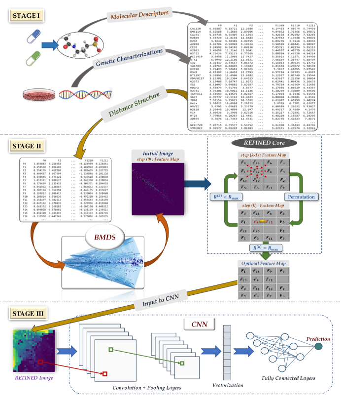
As mentioned earlier, the main idea of the REFINED CNN approach is to map high-dimensional vectors to mathematically justifiable images for training by traditional CNN architecture. Evidently, a mapping of features from the high dimensional vector to a 2-D image matrix serially in a row by row or column by column fashion will not guarantee any spatial correlations in the image. Instead, we first obtain the euclidean distance matrix of the features and use it as a distance measure to generate a compact 2D feature representation where neighborhood features are closely related. A potential solution to achieve this 2-D projection is to apply dimensionality reduction approach such as Multidimensional Scaling (MDS) [20] on a distance measure such as euclidean distance of features. However, that will not guarantee that each mapped point will have a unique pixel representation in the image and might result in sparse images due to the overlap [21]. For instance, if we have 900 features, the features can potentially be represented by a $30\times 30$ matrix and a direct MDS like approach on a $30\times 30$ dimension space might not spread out each feature in such a manner that each pixel contains at most one feature. To ensure that the features are spaced out in a discrete grid and to incorporate the discrete nature of the image pixels, we apply a Bayesian version of metric MDS. We start with the MDS algorithm to create an initial feature map (a 2-D space with feature coordinates) that preserves the feature distances in the 2-D space with minor computational cost. Next, we apply the Bayesian MDS (BMDS) to estimate the feature location on a bounded domain with the constraint that each pixel can at most contain one feature. However, the location of the features are estimated up to an automorphism. Therefore, we apply a hill climbing algorithm, with a cost function that measures the absolute difference in the Euclidean distances among the new feature locations (as represented by the 2D image map) to the estimated true distances ($\hat{\bm{\delta}}$, anticipating the following section) among the features, to arrive at an optimal configuration.

More specifically, starting from the BMDS location estimates, we considered all the configurations in the map sequentially in row-order. For each feature, we tried different permutations of the features by interchanging the position of the central feature position with its neighboring features and selected the permutation that minimizes the above mentioned cost function. Once the cost function is minimized, a set of unique coordinates in a 2D space was produced for each feature. Using those coordinates, we mapped the features into a 2D space and create an image per sample. The created images were then used to train the REFINED CNN.

The general idea of the REFINED CNN approach is shown pictorially in Figure 1 for the application case of predicting drug efficacy over a cell line using genetic characteristics of cell lines and chemical descriptors of the drug as predictors. In Figure 1, an example case is shown where F-12 has been interchanged with its neighboring features, and after each exchange, we checked the similarities/correlation among distances of features from the map and estimated distance matrix of descriptors. If we can find a better exchange case in the feature map, we exchange that feature pair and arrive at a new feature map. The entire process was repeated iteratively until we reached the optimized feature map that is close to the benchmark distance matrix ($\hat{\bm{\delta}}$) of the initial features (in this case PaDEL descriptors).

At the conclusion of this iterative algorithm, we arrive at a REFINED feature map with all features having a unique position in a bounded 2-D space and similar features are placed close by and dissimilar features are far apart. Without loss of generality, we have considered feature maps on unit square and the BMDS specification induced sparsity in the image.

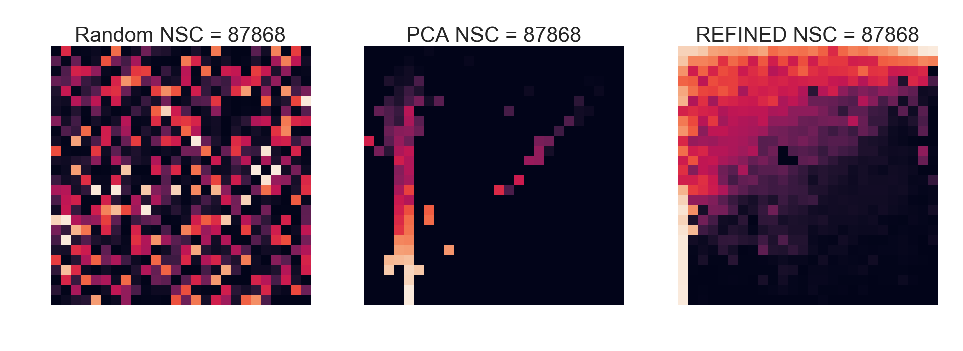
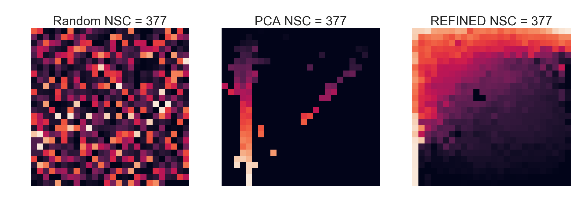
Figure 2 shows some generated REFINED images for different drugs. Each image varies from another depending on the value of the PaDEL descriptors of the drug, but the descriptor coordinates are same for all the cases.

Figure 1: Overview of training a CNN using REFINED images which mainly transforms cell line-drug pairs data structures into images, (STAGE I) distance matrix of the 672 PaDEL descriptors of the cell line-drug pairs are used to calculate the distance between features, (STAGE II) Initial BMDS images generated using the initial distance matrix, then hill climbing algorithm utilized as an iterative optimizer to maximize the correlation between features, by relocating the features (descriptors) in the distance matrix. (STAGE III) A CNN is trained using REFINED images and drug responses of the 60 drugs of NCI60 dataset to predict drug sensitivity of paired cell lines.

Figure 2: Illustration of generated images randomly selected from the NCI60 dataset, where the caption denotes the method that is utilized to generate the image followed by the NSC ID associated with the image.

2.1.1 Theoretical Basis for REFINED

Consider the predictor matrix $\bm{X}=\{x_{ij}\},i=1,2,...,n;\;j=1,2,...,p$ with $x_{ij}$ being the value of the $j$th predictor for the $i$th subject. Suppose, the predictors are generated from a latent zero mean, square integrable stochastic process $\{Z(s)\}$ where the index $s$ belongs to a compact subset of $\mathbb{R}^{m}$. Let $s_{j}$ denote the original position of the $j$th predictor produced by $Z(s)$ and the observed data is randomly permuted version of the original data, i.e. $x_{ij}=Z_{i}(s_{j})$.

Case 1: There is a underlying true ordering of the predictors , i.e., there exists a permutation $\{\pi(1),...,\pi(p)\}$ of $\{1,2,...,p\}$ such that $s_{\pi(1)}<s_{\pi(2)}<...<s_{\pi(p)}$ is the true, but unknown, ordering of the predictors. If such ordering exists, we can take $m=1$ and the predictors can be projected on $[0,1]$ via unidimensional scaling (UDS). Let $\{\hat{s}_{1},...,\hat{s}_{p}\}$ be the estimated locations of the $p$ predictors on $[0,1]$ obtained via UDS. Let $\{\psi(1),...,\psi(p)\}$ be the permutation of $\{1,2,...,p\}$ that orders $\{\hat{s}_{1},...,\hat{s}_{p}\}$. Then under some regularity conditions $\psi(j)=\pi(j),\;1\leq j\leq p,\;\forall p$. Thus UDS can correctly identify the true relative pairwise distances among the predictors.

For proof, see [32].

Case 2: Suppose the ordering does not exist. For example, suppose three predictors are equidistant from one another. Clearly, $m=1$ may not be a valid assumption and results corresponding to Case 1 become untenable in this situation. For the second order approximation, we start with $m=2$, i.e., we would like to obtain the location of the predictors in a compact subset of $\mathbb{R}^{2}$. Without loss of generality, we project the locations on unit square ($[0,1]^{2}$).

Let $d_{jk}$ be the observed distance between the $j$th and the $k$th predictor and $\delta_{jk}$ be their true, but unobserved, distances. Under the assumption of Euclidean metric,$\delta_{jk}=\sqrt{\sum_{l}(s_{j,l}-s_{k,l})^{2}}$, where $s$ is now 2D coordinate system denoting the true location of the predictors $j$ and $k$ in unit square. As in Case 1, we can assume that $\pi(.)$ is the underlying true permutation of 2D configurations of the $p$ predictors. Our goal is to draw inference on the locations of each predictor, i.e. estimate $s_{j}\in[0,1]^{2}$.

[33] developed a Bayesian estimation procedure to estimate $s$ based on observed distance by assuming $d_{jk}\sim N(\delta_{jk},\sigma^{2})I(d_{jk}>0)$ at the data level. For the location process, we specify a spatial Homogeneous Poisson Process (HPP) with constant intensity $\lambda=p/[0,1]^{2}$ which essentially distributes locations of $p$ predictors randomly in an unit square. Since this corresponds to complete spatial randomness, an alternative specification of location process is given by $\bm{s}=\{s_{1},s_{2},...,s_{p}\}\sim Uniform([0,1]^{2})$ [38]. Note that, the properties of HPP guarantee that the HPP operating on the unit square can be further partitioned into disjoint cells and the entire location process can be expressed as the superposition of the HPPs operating on these disjoint cells. Futhermore, as the volume of each cell (within the unit square) goes to zero, so does the probability of observing more than one event in that cell [35]. We also note that, we do not assume that the location process shows any clustering tendency a-priori, however the uniform specification is flexible enough to capture clustering a-posteriori [38]. Let us denote the set of observed and true distances by $\bm{d}$ and $\bm{\delta}$, respectively. Our data model is then given by

$$f(\bm{d}|\bm{s},\sigma^{2})\propto(\sigma^{2})^{-q/2}\exp\left[-\frac{1}{2\sigma^{2}}\sum_{j>k}(d_{jk}-\delta_{jk})^{2}-\sum_{j>k}\log\Phi(\delta_{jk}/\sigma)\right]$$ (1)

where $q$=$p\choose 2$ is the total number of distances in the dataset and $\Phi(.)$ is the usual standard normal cdf. At the process level, we have

$$\bm{s}|p\sim Uniform([0,1]^{2})$$ (2)

Finally, the prior is given by $\sigma^{2}\sim IG(a,b)$ with $a>2,\;\;b>0$ and $IG$ denoting the Inverse Gamma distribution. Consequently, the full posterior distribution is given by

$$[\bm{s},\sigma^{2}|\bm{d}]\propto(\sigma^{2})^{-(q/2+a+1)}\exp\left[-\frac{1}{2\sigma^{2}}\sum_{j>k}(d_{jk}-\delta_{jk})^{2}-\sum_{j>k}\log\Phi(\delta_{jk}/\sigma)-b/\sigma^{2}\right]$$ (3)

When $q$ is large, $\sum\log\Phi(.)\approx 0$, the full conditional posterior of $\sigma^{2}|.$ is approximated by $IG(q/2+a,\frac{1}{2}\sum_{j>k}(d_{jk}-\delta_{jk})^{2}+b)$. However, the conditional posterior of $\bm{s}$ is not available in closed form, a Metropolis-in-Gibbs sampler is used to obtain posterior realizations of the locations. Since $\bm{s}$ are identifiable only up to an automorphism, convergence of the Markov Chain Monte Carlo (MCMC) is assessed on $\bm{\delta}$ and $\sigma^{2}$. Furthermore, following the recommendation of [33], we used the posterior mode of $\bm{s}$ as the point estimate of the predictor location.

Once these locations are estimated, we have a set of point-referenced predictor location in the domain of interest. The domain is then subjected to regular square tessellation such that each pixel contains at most one location – essentially rewriting the point process a-posteriori as superposition of constant intensity local point processes operating on disjoint cells that the unit square in partitioned into. Additionally, the constraint of allowing at most one predictor location per-pixel implies that the posterior location process is approximated by a Non-homogeneous Poisson process [35]. The foregoing hill climbing algorithm is then applied to arrive at locally optimal configuration .

Once the tiled surface associated with the feature space is obtained, we have the observed value, $x(s_{j})$, for each row of $\bm{X}$. The intensity at each pixel is, therefore, determined by $x(s_{j})$. Pixels that do not contain any predictor location are assigned null values. This pixelated image on unit square is our second order approximation of the random functions developed in [32]. We can then deploy any suitable smoothing operation (for example, autoregressive spatial smoothing [34]) to generate the corresponding predictor images (such as shown in figure 2). Furthermore, each posterior realization of $\bm{s}$ can be used for data augmentation purpose in CNN architecture. Also, since Euclidean metric is invariant under translation, rotation and reflection about the origin, any such perturbation will not affect the relationship between the response and predictors.

Note that, even if there exists ordering among the covariates, we can still generate these images in the following way. Since [32] guarantees that the relative pairwise distances among the predictors, estimated from UDS, are consistent estimators of the true relative distances, we can posit a calibration model for these estimates $\hat{d}_{jk}$ to connect with the true distance, i.e. $\hat{d}_{jk}\sim N(\alpha_{0}+\alpha_{1}\delta_{jk},\sigma^{2})I(d_{jk}>0)$.

2.2 Datasets and Preprocessing

To evaluate our framework, we considered three datasets: (a) A synthetically generated dataset (b) NCI 60 dataset consisting of drug responses following application of more than 52,000 unique compounds on 60 human cancer cell lines [22] (c) Genomics of Drug Sensitivity in Cancer (GDSC) [24] dataset that contains responses to 222 anticancer drugs across approximately 972 cancer cell lines with known genomic information. In scenario (b), we use the chemical descriptors of drugs to predict drug responses in a specific cell line. In scenario (c), we consider two heterogeneous predictor set- (i) gene expressions for cancer cell lines and (ii) chemical descriptors for applied drugs and use both these type of predictors to predict drug responses .

(a) Synthetic dataset

We simulated a synthetic dataset with $P$ correlated features for $N$ samples, where for each simulation 20%, 50% and 80% of the features were spurious. The features were simulated from a zero mean Gaussian process with stationary isotropic covariance matrix whose $(i,j)$th element is given by $\gamma^{|i-j|}$. $P$ ranged from $20,50,100,400,800,1000,2000,4000$ and for each P, the number of simulated sampled ranged from ${50,200,600,1000,2000,5000,10000}$. We simulated the target values by simply multiplying random weights to the features. For example, $N$ target values with 100 features ($\bm{X}^{N\times 100})$, with 20% spurious features were generated using the relation $\bm{X}[\bm{\beta}_{r},\bm{\beta}_{0}]^{T}$ where $\bm{\beta}_{r}^{80\times 1}$ are non-zero random weights and $\bm{\beta}_{0}^{20\times 1}$ are zeros.

(b) NCI dataset

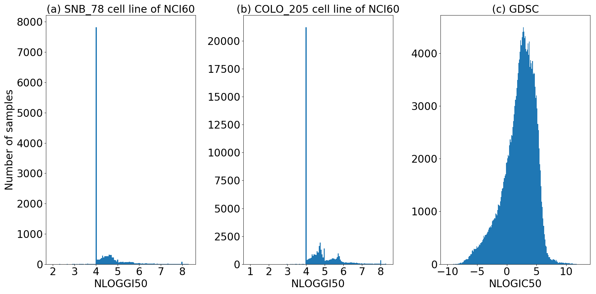
The US National Cancer Institute (NCI) screened more than $52,000$ unique chemicals on around 60 human cancer cell lines. The chemical (drug) response is reported as GI50 which is the concentration required to achieve 50% of maximal inhibition of cell proliferation [22]. All the chemicals have an associated unique NSC identifier number which is assigned to identify agents when they are submitted for clinical trials to the Cancer Therapy Evaluation Program (CTEP). We used the NSC identifiers to obtain the chemical descriptor features and then used PaDEL software [23] to extract these features for each one of the chemicals. The chemicals with more than 10 % of their descriptor values being zero or missing were discarded. The final dataset consists of $52,126$ chemicals, each with 672 descriptor features and 59 cancer cell lines. To incorporate the logarithmic nature of dose administration protocol, we calculated the negative-log concentration of GI50s (NLOGGI50). The drug response distribution for one illustrative cell lines is shown in figures 3 (a). We selected 17 cell lines with more than 10k drugs, to ensure availability of enough data points for training deep learning models. The number of drugs applied on each selected cell line are provided in table 5 of the appendix. All these preprocessing steps were conducted on the training phase.

Figure 3: (a), (b) Drug response distribution of $SNB\_78$ and $COLO\_205$ cell lines of NCI60 dataset in natural logarithmic scale, where all the cell lines response distribution with more than 10,000 samples have the same large peak, (c) represents the drug response distribution in natural logarithmic scale of all the drugs that had been applied on all the cell lines available in the GDSC dataset.

(c) GDSC dataset

For validation of our framework, we also considered the Genomics of Drug Sensitivity in Cancer (GDSC) [24] dataset which describes the responses to 222 anticancer drugs across approximately 972 cancer cell lines. The resulting drug-cell line pairs have the responses reported in the form of IC50 which denotes the concentration of the drug to reduce the response by 50%. The normalized drug response distribution is shown in figure 3(c). We used the gene expression of the cell lines data (17,737 genes), and PaDel descriptors of drug data as predictors. Descriptors with more than 10 % zero or missing values were removed from the dataset, and the rest of missing values were imputed using KNN. Finally, 171K drug-cell line pairs (953 Cell lines, and 206 Drugs) are available for training.

Since in prior drug sensitivity studies [1] [2] [27], an initial feature selection was used to reduce the number of genes before training the predictive model, we also used an a-priori RELIEFf based feature selection [28] for scenario (c) for easier comparison with earlier studies. Since multiple drugs were tested on each cell line, a common subset of 1211 genes were selected that were found to be common among top 8048 $\sim$ 8000 genes selected for each drug. Similar to NCI60 scenario, we used PaDEL software to obtain the chemical descriptor features. The chemical descriptors with more than 10 % of their descriptor values being zero or missing were discarded. Finally each drug has 992 descriptors as features. The gene selection process was conducted on the training set, then the same set of genes were used for validation and test. All the gene expressions and drug descriptors were normalized between 0 and 1.

2.3 Predictive Models

We used the REFINED images to train a CNN regressor to predict drug sensitivity of the NCI60, and GDSC datasets, as well as the simulated target values of the synthetic datasets. We compared performance of the REFINED CNN with Random Forest (RF), Support Vector Regressor (SVR), a deep Artificial Neural Network (ANN) for synthetic dataset. For other datasets, along with RF, SVR, and ANN, we compared the REFINED CNN with Elastic Net (EN), CNN with images created by random 2D projection matrix (Random CNN), and CNN with images created using principal component analysis (PCA CNN) coordinates. The details on Random CNN and PCA CNN are included in section 3.1. We randomly picked 17 cell lines where each cell line contained more than 10k drug responses so that we have sufficient number of samples to train a deep learning model. Subsequently, 17 set of models were trained to predict NLOGGI50 of drugs tested on the selected cell line. In each set, all the above-mentioned models were trained on the same set of samples and tested on a separate set of same samples.

Note that for the synthetic dataset and the NCI60 dataset, the predictors are a vector of real values (chemical descriptor values for NCI60) that are converted to images. For the GDSC dataset, we have two types of input features: chemical descriptors describing the drugs and gene expression describing the cell lines. We generated individual images for each feature type and used both of them as inputs to the CNNs. For the RF, SVR, ANN, and EN these two types of features were appended and used as the predictors. We trained REFINED CNN and 6 other competing models on same set of samples, where each sample is a combination of one drug tested on one cell line. All the models were tested on a separate set of same samples.

The distribution of NLOGGI50 shows a massive point mass at 4 (Figure 3 (a) and (b)) indicating that an overwhelming majority of drugs are not sensitive for majority of the NCI60 cell lines. Thus, we also considered a classification problem of whether a drug is sensitive or resistive among the NCI60 cell lines. Based on the NLOGGI50 distribution for different cell lines, the sensitivity threshold was empirically fixed at 4.5. All the drugs with NLOGGI50 less than the threshold (4.5) were considered resistive and the rest as sensitive. Similar to the regression scenario, we compared the CNN performance with RF, SVM, ANN, logistic regression (LR), Random CNN, and PCA CNN for the classification scenario.

2.3.1 Convolutional Neural Network

Convolutional Neural Networks (CNN) are designed to model multidimensional arrays, where convolutional layers along with pooling layer, are adaptive feature extractors connected to sequential fully connected layers [6]. A convolutional layer consists of multiple kernels connected to a local path of neurons in the previous layer, where all neurons share same parameters to generate a feature map. Thus, all neurons within the feature map scan same features in different locations of the previous layer. The pooling layer summarizes the feature map by finding the maximum/average of each adjacent kernel, which reduces the number of model parameter [5]. We used two different CNN architectures, a sequential CNN for modeling the NCI60 and synthetic dataset, and a hybrid CNN, that can accommodate drug and genetic image for the GDSC datasets.

The sequential CNN regressor contains six learned layers: one input layer, two convolutional layer, two fully connected layer and one output layer. The CNN input dimension is same as the input image dimension, $26\times 26$. The convolutional layer contains 64, $7\times 7$ kernels convolving with valid border mode and stride of 2, followed by batch normalization, and ReLu activation. Each fully connected layer is followed by a batch normalization layer and ReLu activation layer. Number of neurons of the fully connected layers are respectively, 256, and 64. A dropout layer with retaining probability of 0.7 was added before the output layer. The above architecture remains same for Random CNN, PCA CNN and REFINED CNN.

The sequential CNN classifier contains input layer with the same size as the CNN regressor, three convolutional layer with 16 kernels of size $7\times 7$, 32 kernels of size $7\times 7$, and 64 kernels of size $3\times 3$. Each convolutional layer is followed by a batch normalization [54] and a rectified linear unit (ReLu) [53] activation function layer. The third ReLu layer is followed by two fully connected layers with 256 and 64 neurons respectively. Same as the CNN regressor, each fully connected layer is followed by a batch normalization, ReLu and a drop out layer. The CNN classifier architecture remains same for Random, PCA and REFINED CNN. We used adam optimizer to train both the CNN regressor and classifier. The CNN regressor and classifier architecture is shown in figure 37 of the appendix.

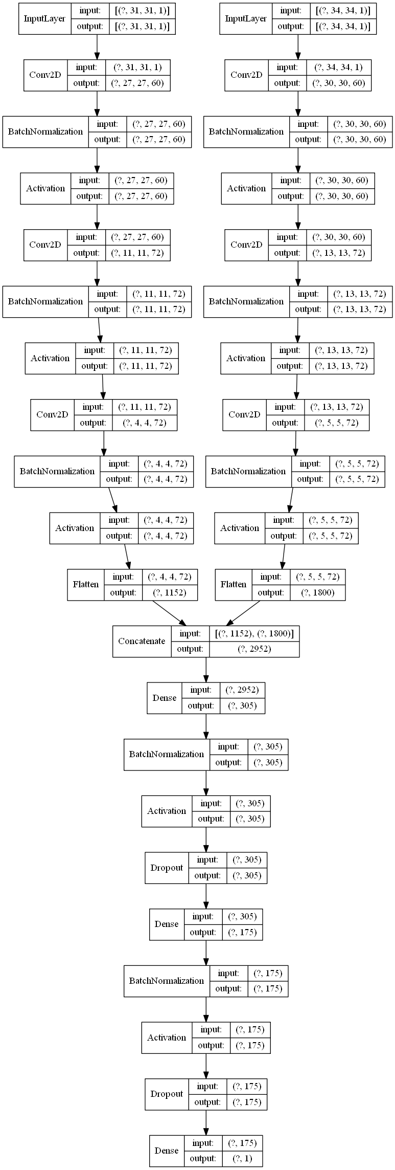
We used hybrid CNNs with two inputs to model GDSC dataset, where two separate images are used as inputs to the two arms of the CNN. Each arm contains three convolutional layers, where the last convolutional layers are concatenated, and followed by two sequential fully connected layers. The two input layers represent the cell lines and drug images, which defines each convolutional layer dimension. The three convolutional layer of each arm have 60 kernels with the size of $5\times 5$ and stride of 1, 72 kernels with the size of $6\times 6$ and stride of 2, and 72 kernels with the size of $5\times 5$ respectively. The last convolutional layer of the arm that takes drug images as the input has stride of 1 and the other arm that takes cell images as the input has a stride of 2. Each convolutional layer is followed by batch normalization and ReLu activation function layers. The last two convolutional arms of the CNN are concatenated and connected to two sequential fully connected layers with 305 and 175 neurons. A batch normalization and a ReLu activation function is included after each fully connected layer. A dropout layer with retaining probability of 0.7 is placed before the output layer. The CNN model architecture is shown in figure 38 of the appendix. The hybrid CNN was trained by an adam optimizer. The same architecture was utilized for Random, PCA and REFINED images. There are some variations in the architecture depending on the training set size that are explained in section 3.4. All tuning parameters were chosen via a comprehensive search that is detailed in the next section.

2.3.2 Hyper parameter search

To tune the competitive models, we did a grid search on the following hyper parameters for each model using hold-out for partitioning the data. We randomly partition both NCI60 and GDSC data to 80 % training, 10 % validation and 10 % test. The same training, validation and test datasets were used for all models. The hyper parameters were tuned using the training and validation sets. The test sets were hold out for evaluating the final performance of each tuned model.

• RF: The number of decision trees in the forest ranged from 100 to 700 trees. For the maximum number of features for the best split evaluated at each node, we tried all the options provided by scikit-learn [52] including: number of features, square root of number of features, and logarithm base 2 of number of features.

• SVM: Gamma parameter of the radial basis function (RBF) kernel using both ’scale’ and ’auto’ options of scikit-learn, and the regularization parameter, ’C’, ranging from 0.01 to 100.

• EN and LR: Alpha penalty term and L1 ratio values between (0.3,0.7) and (1e-6,1e-4), respectively.

• ANN: Number of hidden layers (3-6), number of neurons per each hidden layer and learning rate of the Adam optimizer.

  • 1 hidden layer: 800-1200 neurons

  • 2 hidden layer: 600-1000 neurons

  • 3 hidden layer: 400-700 neurons

  • 4 hidden layer: 200-500 neurons

  • 5 hidden layer: 50-250 neurons

  • 6 hidden layer: 20-80 neurons

  • learning rate: 1e-6 - 1e-3

• CNN: As we did not have access to GPUs, we did not do comprehensive hyper parameter grid search for the CNNs. The current parameters were chosen over about hundreds of run. The hyper parameter space that we searched was number of convolutional layers, number of dense (fully connected) layers, and the learning rate of the Adam optimizer. In each convolutional layer, we seek optimum number of kernels, kernel size, and stride. Per each dense layer, we checked multiple number of neurons. The insights that we gained from thousands of runs are as follows:

  • We observed that $7\times 7$ kernels were better than smaller kernels of 3x3 for the convolutional operator. For larger number of features, larger kernels might be desirable.

  • Using strides larger than 1 is more effective in embedded dimensionality reduction than the pooling layer.

  • Using two or more sequential convolution layers with kernel size of $7\times 7$ and stride of 2 reduces the feature map dimension considerably compared to the input image. Therefore, large number of kernels is recommended at least for the last convolution layer, to provide sufficient number of extracted features for the dense layer.

  • The width of network is as important as the depth of the network.

  • The Adam optimizer is recommended.

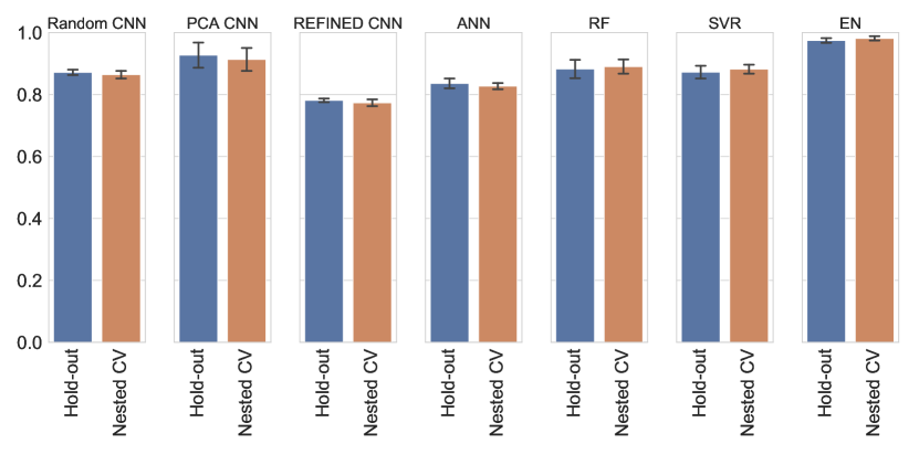
For unbiased evaluation of machine learning models, nested cross-validation [51] (CV) is often considered where an inner CV is used for model selection (hyper parameter selection) and an outer CV is used for evaluating the model tuned by the inner CV. However, nested CV is often extremely computationally intensive and thus we considered a training-validation-test (hold-out) approach where the hyper-parameters are tested on the validation set and the selected model is evaluated based on the separate test set. We used training-validation-test approach as the sample size is relatively large and thus, both training-validation-test and nested CV approaches are expected to provide similar results for comparing different modeling approaches. To illustrate the similar behavior, we compared the results of nested CV and training-validation-test (hold-out) approach using three cell lines randomly selected from the NCI60 dataset. As the results provided in figure 18 indicates, the difference in the results are minimal. On the other hand, to compare the time complexity of the two approaches, we selected one cell line with a fixed CNN architecture. Within the CNN architecture, a grid of hyper parameters was defined. In a single run (architecture) that takes 48 hours on Texas Tech University high performance computer center, 50 different models can be tried using training-validation-test, whereas only 4 models can be tried using nested cross-validation. Given the time complexity and similar performance of the two approaches, we used training-validation-test approach for hyper parameter selection and model evaluation as we could search considerably larger space of hyper parameters.

3 Results

In this section, we report the performance of our REFINED-CNN methodology on the previously described synthetic, NCI60, and GDSC datasets. In each case, the performance of the REFINED CNN was compared to ANN, RF and SVR models. We also compared the REFINED CNN with EN, Random CNN, and PCA CNN for biological datasets.

Evaluation Metric: We evaluated the performance of each regression model using (a) normalized root mean square error (NRMSE), (b) Pearson correlation coefficient (PCC) between the predicted and target values and (c) bias reduction. The NRMSE (4) is the ratio of the root mean squared error (RMSE) of a given model to the RMSE with mean as the predictor. It represents the overall potential of the model to minimize prediction error.

$$NRMSE=\sqrt{\frac{\sum_{i=1}^{N}(y_{i}-\hat{y_{i}})^{2}}{\sum_{i=1}^{N}(y_{i}-\bar{y})^{2}}}$$ (4)

where the $y$, $\bar{y}$ , and $\hat{y}$ are respectively the target data, mean of the target values, and predicted target values. We offer NRMSE in order to implicitly compare all the models with respect to the baseline intercept-only model.

PCC indicates collinearity between the predicted and observed responses. Lack of collinearity often implies model misspecification and lack of predictive capability.

To represent the bias, we first generated the scatter plot of the residual (ordinate) and the observed response (abscissa). We captured the bias via the angle ($\theta$) between the best fitted line through the residuals and the abscissa. An unbiased model is expected to produce an angle of $0^{\circ}$. Therefore, a smaller value of $\theta$ indicates that the model is less biased.

We used Gap statistics [41] to report the significance of the difference in performance across methods of the regression tasks. We paired each model with a null model [1] with bootsrap sampling, where the bootstrap sampling was done on the dose-response values of the test set along with their corresponding predicted values for each model and the null model randomly predicted dose-response values for the sampled test set using the distribution of the training set dose-responses. The process is repeated for 10,000 times and a distribution of NRMSE, PCC, and Bias, is made for each model along with the null model. The distribution per each metric for each model is paired with null models’ metric distribution. Then cluster centroids are calculated using K-means (k = 2) clustering, after the Gap statistics shows appropriateness of using 2 clusters. The difference between each model and the null model cluster centroids per metric represents the difference between them. In addition to the Gap statistics, all models were subjected to a robustness analysis [1], where we calculate how many times the REFINED CNN outperforms other competing models in 10,000 repetition of bootstrap sampling process.

We calculated 95 % confidence interval for each metric that is used to measure the performance of the methodologies in modeling NCI60 and GDSC dataset using a psuedo Jackknife-After-Bootstrap confidence interval generation approach [4, 31]. Multiple Bootstrap sets were selected from the test samples and error metrics generated resulting in a distribution for each error metric which was used to calculate the confidence interval for a given cell line for NCI60 dataset or a given pair of cell line and drug for the GDSC dataset.

The classification models that predict the sensitive and resistive drugs applied on the NCI60 data cell lines, were evaluated using accuracy, precision, recall, F1 score, and area under the receiver operating characteristic curve (AUROC) metrics. Accuracy is the ratio between correct predictions; true positive (TP) and true negative (TN), over all the predictions; summation of TP, TN, false positive (FP), and false negative (FN).

$$Accuracy=\frac{TP+TN}{TP+TN+FP+FN}$$ (5)

Precision is the ability of predicting positive instances of the classifiers, or in other words, the ratio of correctly predicted positive instances.

$$Precision=\frac{TP}{TP+FP}$$ (6)

Recall or true positive rate (TPR) is the ability of the classifiers in predicting positive instances, which corresponds to the proportion of of positive instances that are correctly predicted as positive.

$$Recall=\frac{TP}{TP+FN}$$ (7)

F1 score is simply harmonics mean of the precision and recall,

$$F1score=\frac{2TP}{2TP+FP+FN}$$ (8)

False positive rate (FPR) is a ratio between negative instances that are mistakenly predicted as positive instances. AUROC combines TPR and FPR in many different threshold for each classifier on a single curve, where the area under the curve is considered as AUROC.

$$FPR=\frac{FP}{FP+TN}$$ (9)

The 95 % confidence interval of each of the above-mentioned classification metrics was calculated using the Binomial proportion confidence interval [42, 43].

3.1 Comparison with other image generation methods

In this section, we consider two alternative image generation methods for comparison purposes: random projection-based and PCA-based. In the random projection method, we assume each image is a matrix and the location of each entry in the vector is randomly mapped to a location in the matrix. Thus, we placed each element of the drug descriptors or the gene expression on the image (matrix) coordinates one after another.

Principal component analysis (PCA) [26] is mainly used for dimensionality reduction and visualization purposes, where each sample could be represented on a 2D plane aligned with their first two principal eigen vectors. The first two principal components of the transposed covariance matrix with rows being features and columns representing samples, were selected as the feature coordinates. Some of the generated images using the random and PCA methods are shown in figure 2.

3.2 Synthetic Data

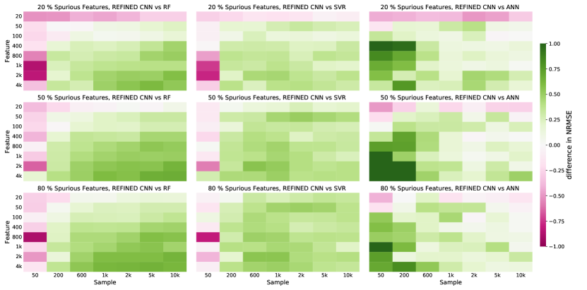
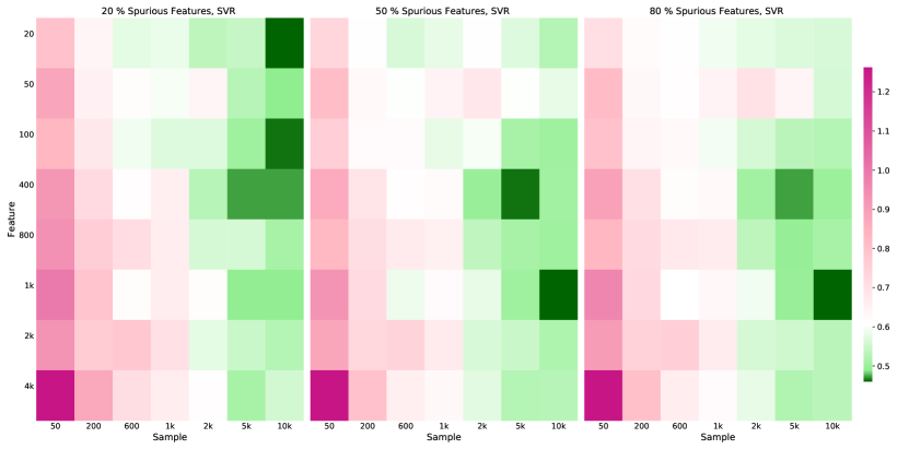
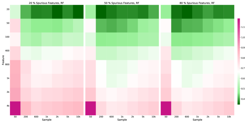
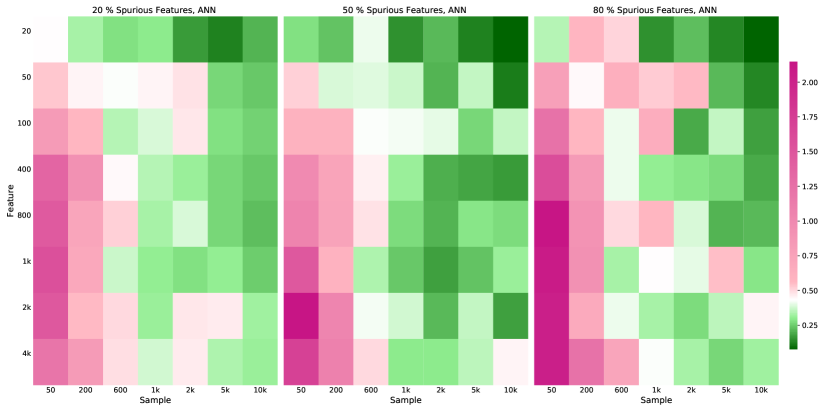
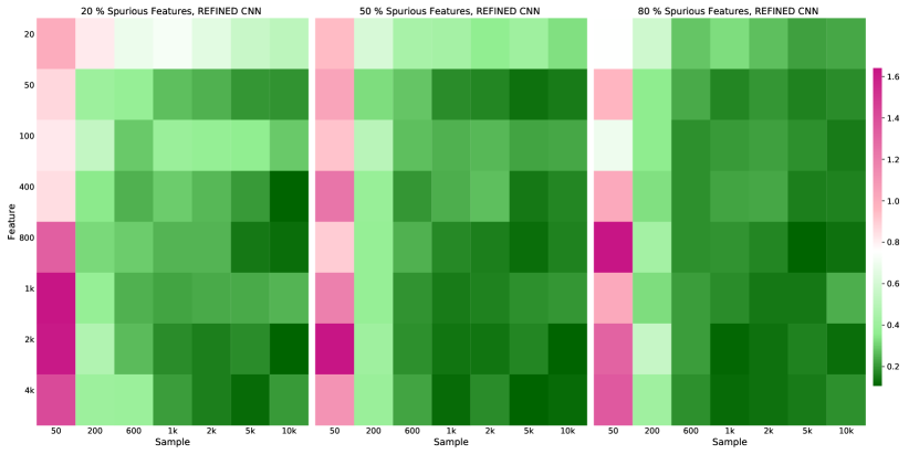
In this section, we offer the comparative performance of the candidate models on the simulated dataset. First we generate a lexicographic ordering of $P$ features. The features are then generated from a $0$ mean Gaussian process with covariance depending only on the lexicographic distance between the features. In each case, a subset of features were randomly selected as spurious. Subsequently, random weights generated for non-spurious features were used to generate the target values. The generated target values were normalized between 0-1. We have used REFINED to generate images for different $N/P$ scenarios and then trained a CNN for each scenario. In each case, the same dataset was used to train RF, SVR and ANN for comparison. We used five-fold cross validation for all the models on fixed training, validation and test sets. The results are summarized in figure 4, as heat maps. As shown in figure 4, the green regions represents the cases where the REFINED-CNN NRMSE is less than the competing models. The separate heatmap for all the model results are provided in the figures 13,14,15,16 of the appendix. The heat maps clearly shows, that the REFINED-CNN methodology outperforms others when the number of features and samples are relatively high ($P>100,N>600$) regardless of the percentage of spurious features present in the dataset. We also observe that the performance of the posited methodology improves as the $N$ increases. [32] also reported that the performance of their UDS based projection improved with increase in both $N$ and $P$. Therefore, our findings suggest that our second order REFINED approximation are in agreement with the first order stringing approximation of [32]. Furthermore, we also observe that as the ratio of spurious features increases, the predictive performance of our REFINED-CNN also improves as compared to the competing models. Recall, we are not performing any feature pre-selection for REFINED-CNN for the synthetic data. This exercise demonstrates the ability of our approach to automatically remove spurious features without performing an explicit feature selection a-priori. Additionally, by comparing the REFINED CNN versus ANN heatmap we observe that increasing the number of samples reduces the gap between their performance as more samples are available to train the large number of parameters of ANN.

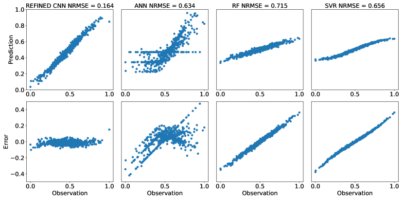
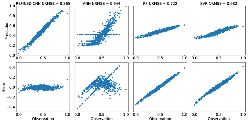
We next investigated the effect of the REFINED-CNN approach on the bias characteristics of the prediction. Figure 17 shows the scatter plot of prediction versus actual responses of the four models when 80 % and 20 % of the features are spurious. Clearly, the scatter plot for REFINED-CNN closely follows a straight line with unit slope indicating predictive accuracy of our approach. RF and SVR reveal their well-known tendency to under-predict higher valued observation and over-predict lower valued observations [17]. REFINED-CNN bias is also better than the bias observed for the ANN scenario. Thus, it appears that the REFINED-CNN approach can automatically improve the prediction bias which some of the other existing models are known to suffer from.

Figure 4: NRMSE difference of REFINED CNN with RF, SVR and ANN for different sample sizes and with different number of features where the 20 %, 50 % and 80 % of the features are respectively spurious. The green regions of each heatmap represents where REFINED CNN outperform other models.

3.3 NCI60 dataset

3.3.1 Classification

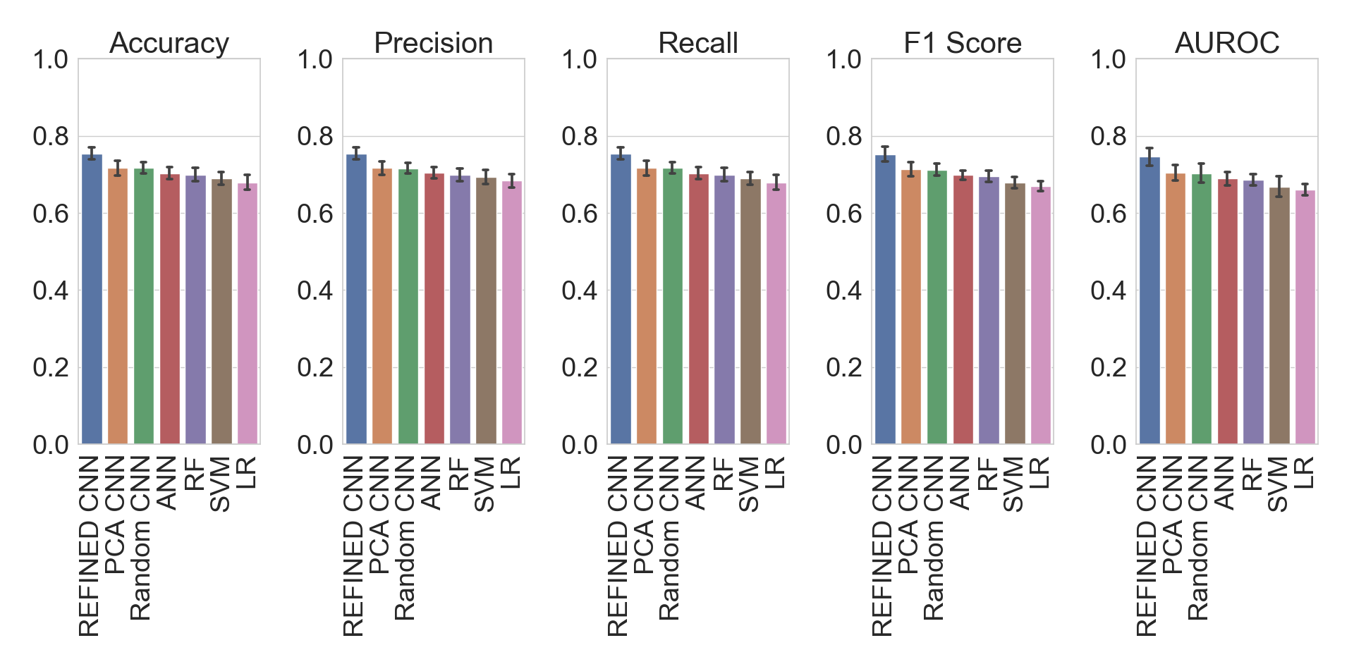
We investigated the discriminative power of REFINED-CNN as compared to other models in predicting resistant and non-resistant drugs on different cell lines of the NCI60 dataset. The threshold for defining resistant and non-resistant classes, was selected based on the drug response distribution shown in figure 3. The drugs with NLOGGI50 smaller than $4.25$ was considered resistant and the rest as non-resistant. Since, we have sufficiently large number of drugs for each cell line , we randomly considered 80% of the drugs for training, 10% for validation and 10% for testing. As shown in the figure 5, the REFINED CNN outperforms other classifiers for all 17 cell lines. The average classification accuracy of REFINED-CNN was 75.4% - considerably higher than the average classification accruacy obtained for Random CNN (71.6%), PCA CNN (71.7%), ANN (70.3%), RF (70%), SVM (69%) and LR(67.9%). For each model, we also report precision, recall, f1-score, and AUROC. REFINED-CNN outperforms other models considering all the metrics. Detailed classification results are provided in appendix tables 6, and 7. The 95 % intervals for each metric for different cell lines are provided in table 9 of appendix.

Figure 5: Summary of REFINED-CNN and 6 other competing classifier models performance on randomly selected cell lines of NCI60 database, using the accuracy, precision, recall, f1-score, and AUROC metrics.

To compare the statistical significance of the difference in performance between competing classifiers and REFINED CNN, we used the McNemar’s test which is a paired nonparametric statistical hypothesis test. McNemar’s test evaluate whether two models disagree in the same way or not. To compare classifiers with REFINED CNN classifier pairwise, a contingency table is formed and McNemar’s test is applied [40]. The null hypothesis is whether two classifiers disagree by the same amount. Therefore, if the p-value is smaller than a threshold (0.05), null hypothesis is rejected, and the conclusion is: there is a significant disagreement between the two classifiers. The results of comparing REFINED CNN with other models using McNemar’s test is provided in table 8 of the appendix. We observe that the REFINED CNN classifier performance is significantly different than the other classifiers (LR, RF, SVM, ANN, Random CNN, PCA CNN).

3.3.2 Regression

The NCI60 dataset was randomly partitioned into 80% , 10% , and 10% segments for training, validation and test purpose, respectively. The same training, validation and test set were used for model comparisons. The performance of each model was evaluated using normalized root mean square error (NRMSE), Pearson correlation coefficient (PCC), and bias.

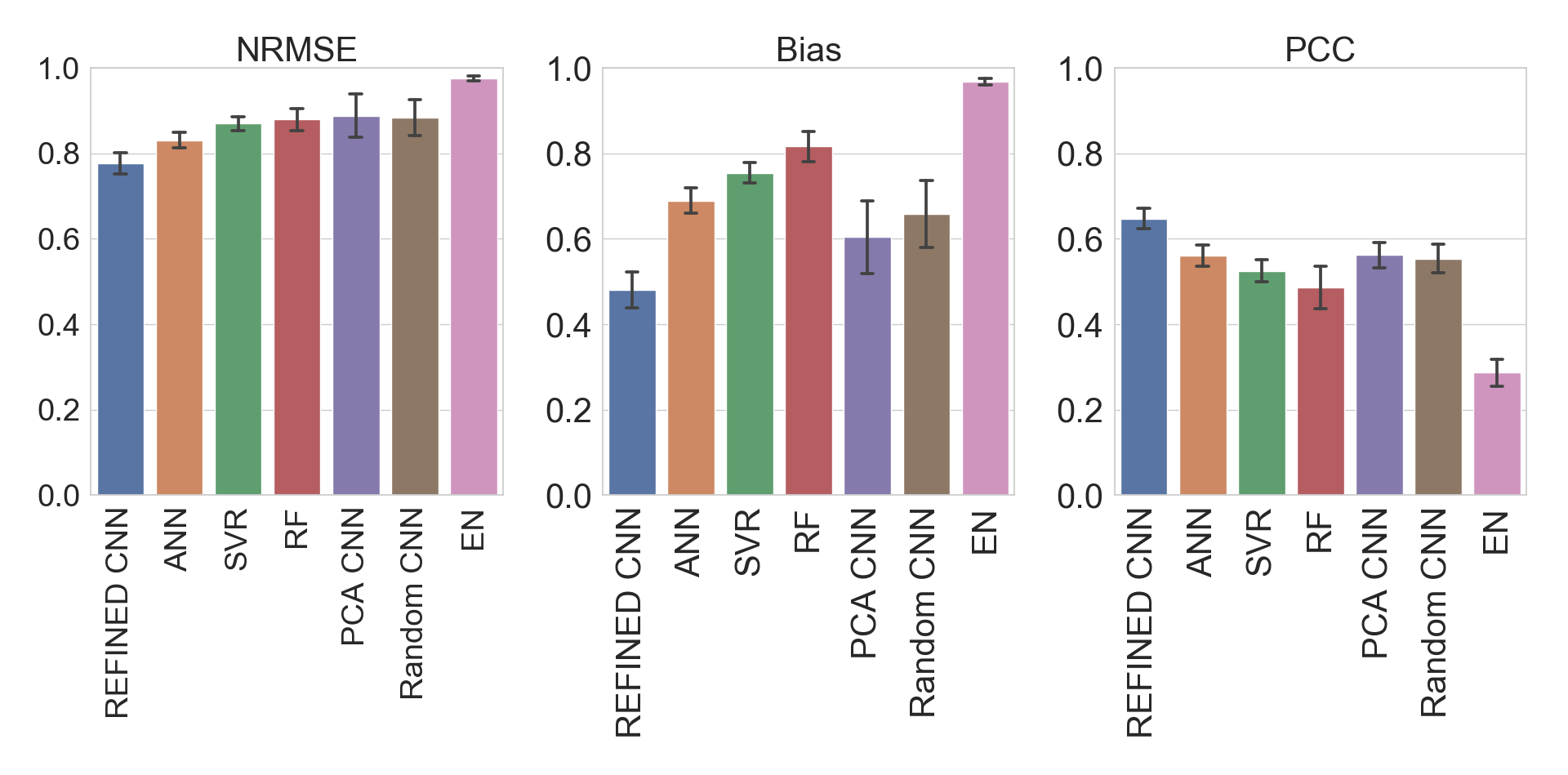
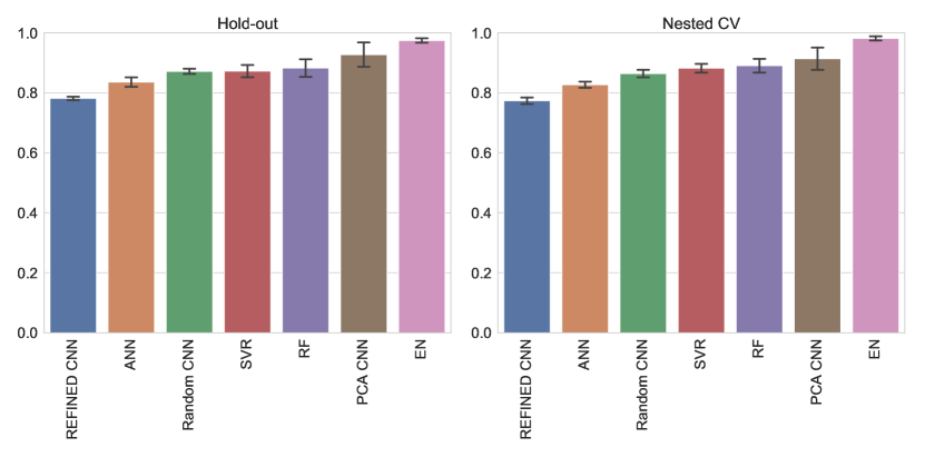
Table 10 in the appendix details the performance of each model with respect to the foregoing metrics for different cell lines. Table 10 is summarized in figure 6, as bar plots. The 95 % confidence interval for all the models per each cell line is provided in the figure 20 21 22 of the appendix. We note that CNN outperforms all the competing models in all 17 cell lines. The average improvement in NRMSE, PCC and bias for REFINED-CNN as compared to other competing models are 6-20%, 8-36%, and 12-38%, respectively .

Figure 6: Summary of REFINED-CNN and 6 other competing regressors models performance on randomly selected cell lines of NCI60 database, using the NRMSE and Pearson correlation coefficients metric.

We used Gap statistics and robustness analysis as described in the evaluation metric section to compare REFINED CNN with other competing models for the regression task. The robustness results are provided in table 11 of the appendix which indicates that REFINED CNN has better performance in terms of: NRMSE between 89.51-100% of the times, PCC between 94.42-100% of the times, and Bias 91.14-100% of the times on average as compared to other models. The Gap statistics results are provided in table 12 of the appendix, which indicates superior performance of REFINED CNN as compared to the other models in all the metrics both in average and per each cell line. The NRMSE and PCC distribution of all the seven models along with the null model are plotted for three cell lines of the NCI60 dataset in figure 19 of the appendix.

3.3.3 Data Augmentation

This section analyzes the effect of augmenting the dataset using samples from the less represented regions. As shown in figure 3(a), the massive point mass associated with the non-sensitive (resistant) drugs severely impacts a global regression model for NLOGGI50. This problem is analogous to zero-inflation problem in classical statistical literature. In such situation, the discrete point mass is modeled separately from the continuous part (see [37, 39] and references therein). In our situation, it boils down to classification into sensitive/resistive category followed by a regression in the sensitive category.

We have already demonstrated superiority of REFINED-CNN in both classification and regression in Tables 6 and 10, respectively. In this section, we explore if REFINED-CNN’s performance could be improved by synthetically oversampling the sensitive category to arrive at a more balanced dataset [36]. To that end, we used a version of SMOTE technique and generated bootstrap replicates from the sensitive category. The NRMSE and NMAE (Normalized Mean Absolute Error) improvement of REFINED-CNN regression model on different cell lines is illustrated in table 1. The bootstrap data augmentation systematically decreases the NRMSE and NMAE for the cell lines indicating the negative impact of the point mass in the response distribution.

Table 1: REFINED CNN NRMSE and NMAE improvement by data augmentation of the sensitive drug region using bootstrap sampling.

	No data augmentatoin			Bootstrap
Cell Lines	NRMSE	NMAE	# Samples	NRMSE	NMAE	#Samples
SNB_78	0.784	0.713	13940	0.744	0.688	19613
MDA_MB_435	0.787	0.739	36868	0.762	0.729	59570
NCI_ADR_RES	0.798	0.745	37156	0.755	0.717	59250
786_0	0.752	0.688	49344	0.713	0.663	76908
COLO_205	0.741	0.664	48946	0.722	0.660	75158

3.3.4 Sample Size Analysis

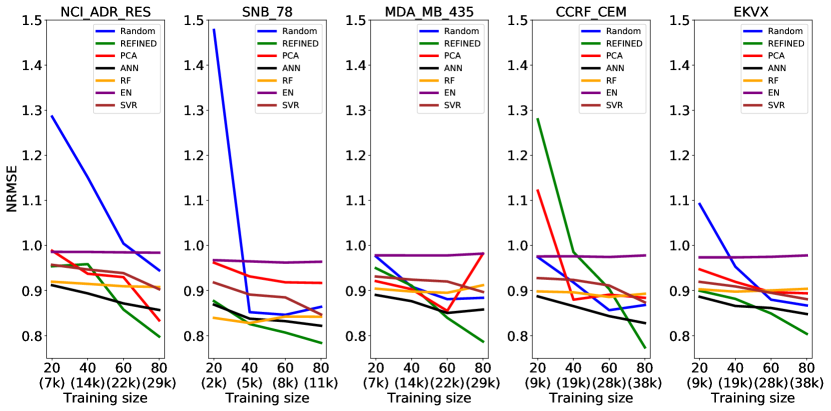
Deep CNN models are expected to perform better with larger number of samples as compared to smaller number of samples. Therefore, we trained our model on different portion of training sets for randomly selected cell lines to test this hypothesis. We trained our model on 20 %, 40 %, 60 % and 80 % of the available drugs applied on the selected cell lines and kept rest of the data for testing, considering NRMSE as a comparison metric. The results of five cell lines are summarized in figure 7 which illustrates that REFINED-CNN outperforms the other models as sample size increases. This trend was also observed on the synthetic data (figure figure 4).

Figure 7: Comparison of six competing models with REFINED CNN for different training sizes applied to five randomly selected cell lines of NCI60 dataset. The x-axis represents the percentage of data used for training of each cell line along with the actual number of samples used in brackets. To fit the figures, we shortened REFINED CNN as REFINED, Random CNN as Random, and PCA CNN as CNN in the legends.

3.3.5 Model Stacking

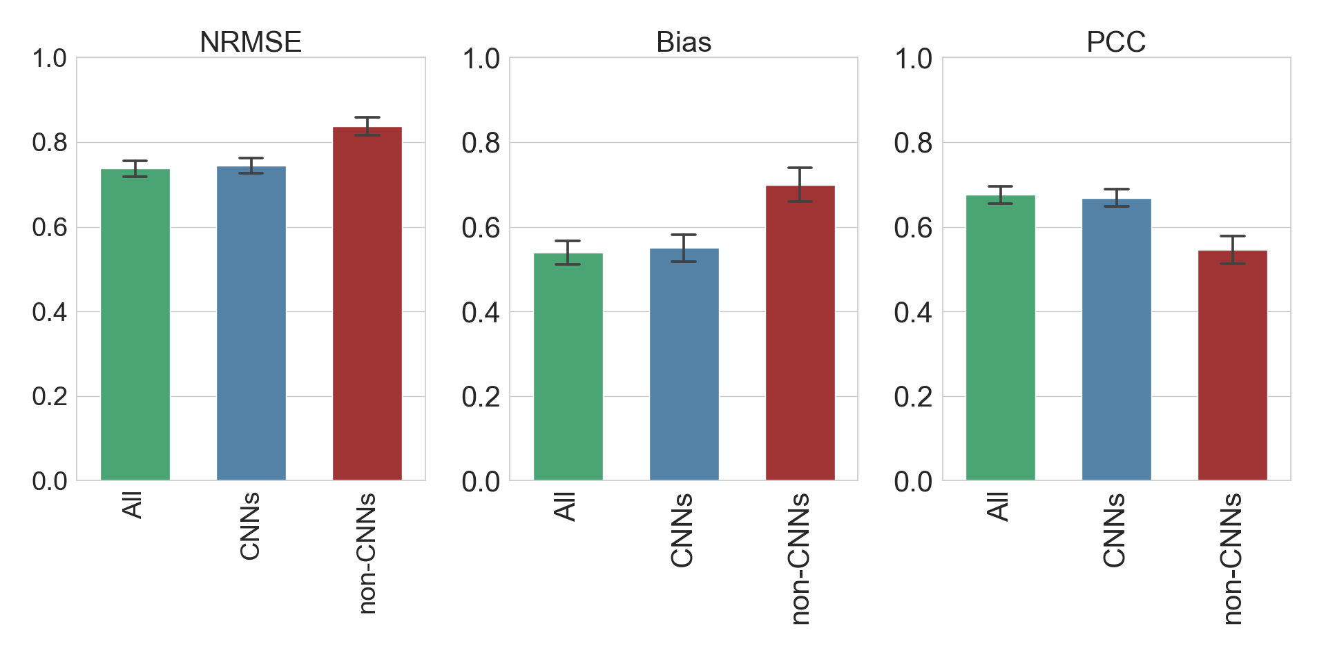
To explore whether stacking of multiple models can improve prediction performance, we stacked predicted drug sensitivity of the validation set of all models–in three different combinations–as the covariates in a linear regression model to find the weight of each model which are then employed to predict drug sensitivity of the test set. These three combinations are stacking non-CNN models (RF, SVR, ANN, and EN); stacking CNN models (PCA CNN, Random CNN, and REFINED CNN); and stacking all models (REFINED CNN and 6 other competitors). Figure 8 represents the stacking results where the average NRMSE of stacking all models is 0.738, stacking CNNs is 0.744 and stacking non-CNNs 0.837. By comparing the stacking results, with average NRMSE of each model in table 6 , the stacking produced a significant improvement as compared to non-CNN models individually. It is notable to mention that REFINED CNN average NRMSE in table 6 is significantly lower than stacked of non-CNN models.

Figure 8: Comparison of stacking all models, all CNN models and non-CNN models using NRMSE, bias and Pearson correlation coefficients (PCC).

3.3.6 Bias Analysis

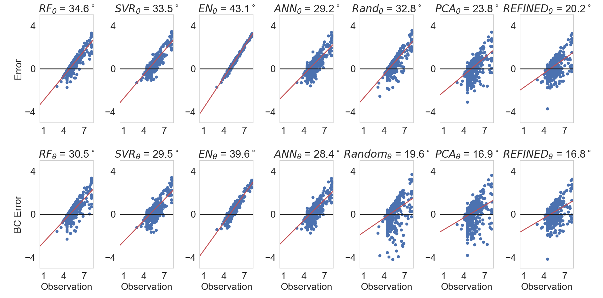
In this section, we re-investigate the effect of the REFINED-CNN approach on the bias characteristics of the prediction using actual biological data. Figure 9 shows the plot of the residuals against the observed values. Similar to the earlier presented synthetic data scenario, Figure 9 (a) shows that REFINED-CNN has the lowest bias ($20.2^{\circ}$) as compared to Random-CNN ($32.8^{\circ}$), PCA-CNN ($23.8^{\circ}$), ANN ($29.2^{\circ}$), RF ($34.6^{\circ}$), SVR ($33.5^{\circ}$) and EN ($43.1^{\circ}$). To investigate whether bias correction erodes the advantage of REFINED-CNN in terms of bias, we considered BC1 bias correction algorithm proposed in [29] where we fit a second model (linear regression was used in this case) on the residuals. The results shown in Figure 9 (b) illustrate the superiority of REFINED-CNN in terms of lowering bias even after bias correction is applied to the competing models.

Figure 9: Residual plots for RF, SVR, EN, ANN, Random CNN, PCA CNN, and REFINED CNN for $SNB\_78$ cell line test set data prior bias correction (BC) (a) and post bias correction (b). The corresponding NRMSE for scenario (a) are RF = 0.842, SVR = 0.847, EN = 0.964, ANN = 0.822 , Random CNN = 0.864 , PCA CNN = 0.917, REFINED CNN = 0.784 and for scenario (b) are RF = 0.830, SVR = 0.836, EN = 0.937, ANN = 0.817 , Random CNN = 0.832 , PCA CNN = 0.840, REFINED CNN = 0.763.

3.4 GDSC dataset

In this section, we consider the application of REFINED CNN in integrating two types of heterogeneous datasets. Our predictors now consist of (a) PaDel chemical descriptors representing the drugs and (b) gene expression profiles for each cell line. The response consists of the experimentally obtained IC50 for each drug-cell line pair. We used the REFINED approach to generate the images corresponding to the gene expressions for each cell line and drug descriptors for each drug compound in the GDSC dataset.

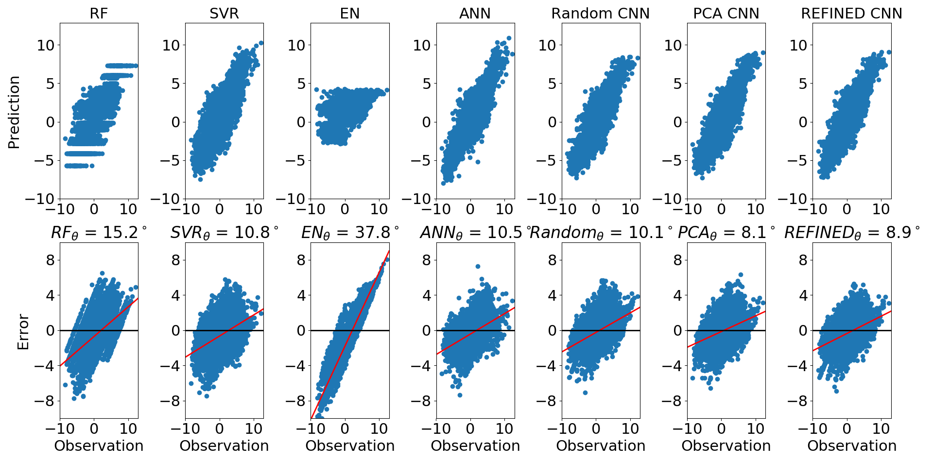
Considering 222 drugs and around 972 cell lines for each drug, the total number of samples in the dataset is close to 177K. We randomly divided the dataset into 80% training, 10% validation and 10% test sets, where each set covariates contains 1211 genes and 992 chemical drug descriptors. Figure 10 represents the scatter plot of the natural log IC50 prediction using our REFINED CNN approach, Random CNN, PCA CNN, ANN, RF, SVR, and EN along with their corresponding residual plots. Table 2 summarizes the performance of each model using NRMSE, PCC, and bias.

Similar to NCI60 data analysis, we used Gap statistics and robustness analysis for further comparison of the models. The robustness analysis and Gap statistics results are provided in tables 16 and 17 of the appendix respectively. The Gap statistics distribution plots per each metric of each model paired with the null model along with their corresponding cluster centroids are provided in figures 30-32 of the appendix.

As shown in table 2, REFINED-CNN model achieves improvement as compared to other models in the range of 1-47% for NRMSE, 1-42%, for PCC. We also train the REFINED CNN on 50% and 20% of the GDSC data and compared it with other competing models. As the CNN architecture (please see figure 38 of the appendix) trained on the 80% of the REFINED images was too complex to be trained on the 20% of the data, we reduced the network complexity of REFINED CNN and ANN models. We removed the last convolutional layer and its latter dense layer for the CNN model, and also we removed the first two dense layer of the ANN model. The detailed corresponding results are provided in table 10. The predicted and residual scatter plots are provided in figures 28, 29 of the appendix.

Table 2: Comparison of REFINED CNN, Random CNN, PCA CNN, ANN, RF, SVR, and EN peformance on the GDSC dataset in terms of NRMSE, Pearson Correlation Coefficients (PCC), and bias

Models	Trained on 20 %			Trained on 50 %			Trained on 80 %
	NRMSE	PCC	Bias	NRMSE	PCC	Bias	NRMSE	PCC	Bias
EN	0.890	0.488	0.848	0.889	0.484	0.849	0.887	0.486	0.840
RF	0.609	0.797	0.433	0.620	0.785	0.417	0.569	0.821	0.337
SVR	0.750	0.847	0.257	0.742	0.845	0.273	0.525	0.853	0.241
ANN	1.407	0.519	0.784	0.475	0.883	0.153	0.435	0.901	0.233
Random CNN	0.579	0.836	0.215	0.456	0.892	0.193	0.441	0.903	0.222
PCA CNN	0.612	0.820	0.201	0.461	0.891	0.228	0.443	0.901	0.179
REFINED CNN	0.541	0.845	0.255	0.439	0.899	0.173	0.414	0.911	0.197

Figure 10: Scatter plot of predicted NLOGIC50s and their residual (error) for each model, in the case of models were trained on 80 % of the available data. In each scatter plot, observation is the NLOGIC50 values if the test set. On the bottom row, bias of each model is depicted by the method explained in the bias analysis section.

We also incorporated larger number of genes to experiment the impact of creating larger images using REFINED. We selected larger common subset of genes including (2147 $\sim$ 2000, 2985 $\sim$ 3000, 4271 $\sim$ 4000, 8048 $\sim$ 8000) genes and created the REFINED images to train the same CNN architecture that we used to train the GDSC data with 1211 selected genes. We also trained other competing models with the same hyper parameters. In our experiment, the SVR model crashed after several hours due to the larger memory requirement while estimating the kernel by computing the distance function between each point in the dataset. Thus, we used a bag of SVRs, where we selected subset of 400 features (appended gene expression and drug descriptors) to train 100 SVRs in parallel. The complete results are provided in figure 33 and table 18 along with the corresponding confidence intervals in figure 34 35 36 of the appendix. We observed that the trend of REFINED CNN outperforming other approaches is maintain irrespective of the number of genes used for training models.

3.4.1 Comparison with state-of-the-art methods

We have also compared REFINED-CNN with another state-of-the-art approach, Deep-Resp-Fores (DRF) proposed by Su et al. [48]. The DRF is a deep cascaded forest model, designed to classify the anti-cancer drug response as “sensitive” or “resistive” based on integration of heterogeneous input data (gene expression and copy number alteration (CNA) of GDSC data. We switched the random forest classifier of the DRF to a regressor for prediction and used drug descriptors in the DRF’s wing that takes CNAs as the input for training the DRF.

We have also compared REFINED-CNN with heterogeneous graph neural networks (HGNN) proposed by Lim et al. [50]. HGNNs automate feature engineering task by aggregating feature information of neighborhood nodes, where the input data of the network are from different sources [49]. Lim’s network embeds the 3D structural information of protein-ligand complexes in distance matrix, to predict drug-target interaction. We trained their network by encompassing gene-drug information in distance matrix, to predict drug sensitivity of the GDSC dataset. The results of applying DRF[48] and HGNN [50] are provided in table 3 for comparing with REFINED CNN. As the results indicate, REFINED CNN outperforms DRF and HGNN for drug response prediction of the GDSC dataset. The robustness analysis and Gap statistics results for both DRF and HGNN methods are provided in the table 16 and 17 of the appendix, respectively.

Table 3: Comparison REFINED-CNN with DRF and HGNN for GDSC drug sensitivity prediction.

Models	NRMSE	PCC	Bias
REFINED-CNN	0.414	0.911	0.197
DRF [48]	0.986	0.169	0.976
HGNN [50]	0.637	0.805	0.446

3.5 Ablation study

The main components of REFINED are dimensionality reduction followed by a search optimization algorithm, where we use Bayesian MDS as a global distortion minimizer and hill climbing as local adjustment to reach a locally optimal configuration among multiple automorphs. To investigate the contribution of each individual component to REFINED, evaluated the effect of different approaches in each step. For the dimensionality reduction step, we considered other dimensionality reduction techniques such as Isomap [44], Linear Local Embedding (LLE) [45], and Laplacian Eigenmaps (LE) [46] instead of Bayesian MDS. Isomap generalizes MDS with using Geodesic distance rather than Euclidean distance in nonlinear manifolds, where the Geodesic distance is approximated by summation of Euclidean distances. LLE is a local dimensionality reduction technique, which tries to reconstruct each sample based on k-nearest samples in a lower dimension locally. Laplacian eigenmap (LE) is similar to LLE except, it uses Laplacian graph to reconstruct k-nearest neighbor, where k eigen vectors corresponding to the k smallest eigen values are preserved for embedding [47].

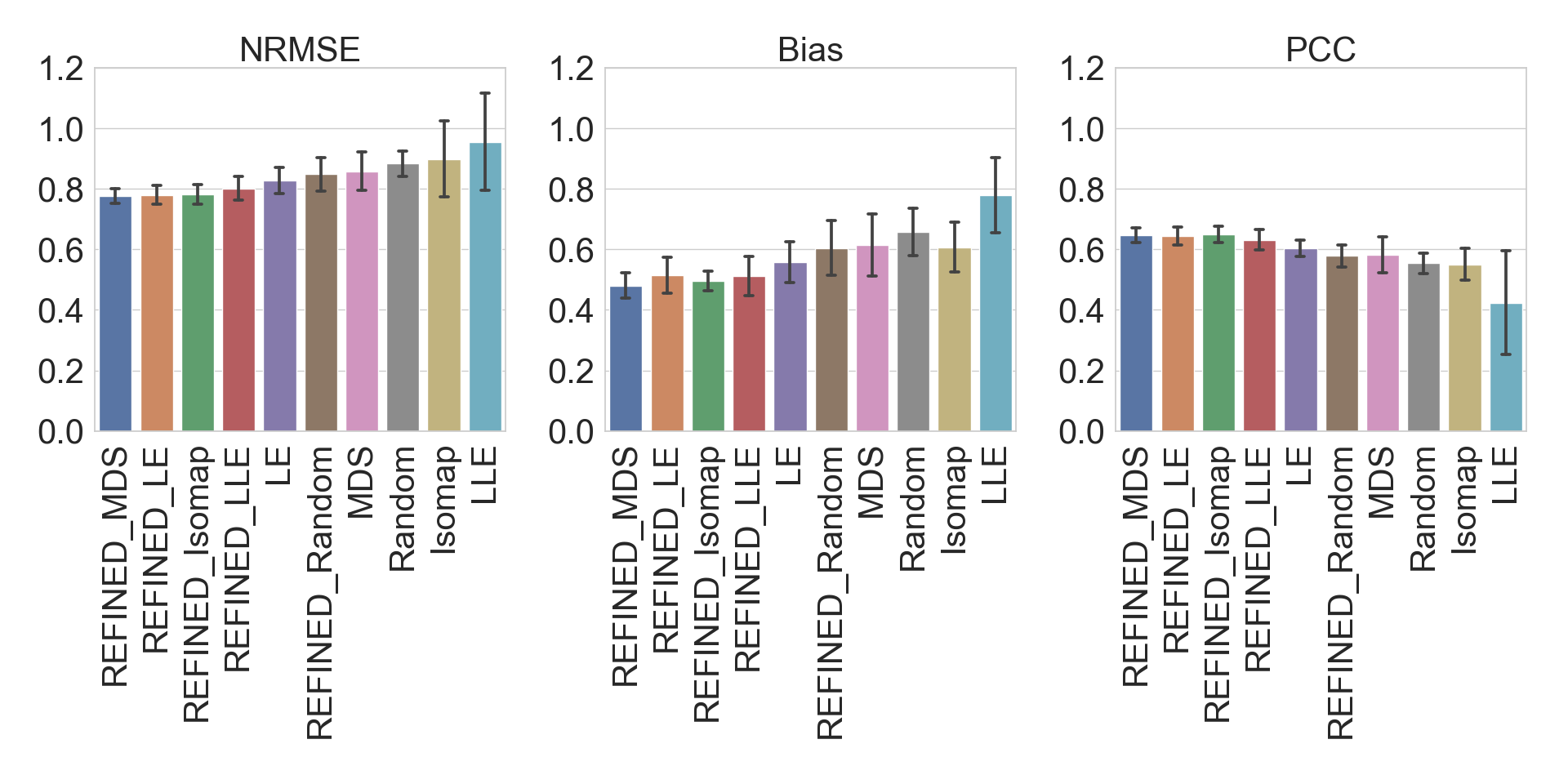
To investigate the contribution of the search optimization algorithm, we initialized each feature location randomly and applied the hill climbing methodology with the objective of minimizing the difference between features Euclidean distance matrix in the initial domain and the created REFINED image. We generated images using all the above-mentioned methods and then trained the same CNN structure that we had used for NCI regression task on the same cell lines. As an example, figure 12 shows created images using each described method for one of the randomly selected drugs of the NCI dataset. Further examples are provided through figures figs. 23, 24, 25, 26 and 27 in the appendix.

The average results are numerically presented in table 4 and the pictorial representation is included in figure 11 as barplots. As the results in the table 4 indicate, NRMSE associated with REFINED initialized with Bayesian MDS is smaller than the NRMSE of all other approaches. We observed that both global and local embedding do better than random initialization followed by hill climbing. We also observed that the idea of non-overlapping pixel locations for the features borne out by the hill climbing step improves the performance if the dimensionality reduction approaches. Complete results of ablation study are provided in table 14 and 15 of the appendix.

Figure 11: Barplots of REFINED ablation study on NCI regression task using three metrics: NRMSE, PCC, and bias, where the bars show the CNN performance for different image generation methods.

Figure 12: Illustration of generated images of a randomly selected drug (NSC = 3069) of NCI dataset, where the first row represent pattern of images generated only with different initialization approach that included overlapping features and the second row shows the REFINED images initialized with different dimensionality techniques followed by a hill climbing step for avoiding overlap among features.

Table 4: Average results of REFINED ablation study on NCI regression task, where the images are generated using different initialization methods with and without applying the hill climbing component.

Initialization	No hill climbing			REFINED
	NRMSE	PCC	Bias	NRMSE	PCC	Bias
Isomap	0.900	0.551	0.608	0.783	0.649	0.496
Bayesian MDS	0.858	0.582	0.616	0.776	0.647	0.481
LLE	0.956	0.424	0.780	0.802	0.632	0.512
LE	0.829	0.603	0.558	0.781	0.645	0.514
Random	0.884	0.554	0.659	0.849	0.578	0.605

4 Discussion

This paper presents a novel approach of converting high dimensional vectors into images with spatial neighborhood dependency that can be used as inputs to traditional Convolutional Neural Networks. The proposed methodology was conceived from the observation that deep learning CNN has increased the prediction accuracy in many scenarios especially when the inputs are images, but it is not usually appropriate when high dimensional vectors with limited neighborhood correlations are used as inputs. Our REFINED approach produces a mapping of the input features such that spatial neighbors are close and far away points in the map are distant in initial feature space.

There are several advantages of the proposed REFINED methodology. First, the REFINED mapping to a compact image space appears to allow for automated feature extraction using deep learning CNN architecture. Using a synthetic dataset and altering the amount of spurious features, we observed that REFIEND-CNN is able to significantly outperform other approaches for scenarios with larger percentage of spurious features as shown in figure 4.

Second, the REFINED CNN approach provides a gain in predictive accuracy as compared to other commonly used predictive models of Artificial Neural Networks, Random Forest, Support vector Machines, and Elastic Net. We have validated the performance of REFINED-CNN in (a) synthetic dataset, (b) NCI60 drug response dataset and (c) GDSC dataset that combines chemical descriptors of drugs with genomic expressions of cell lines. REFINED CNN also outperforms other state of the art methods such as Deep-Resp-Forest and Heterogeneous graph models. REFINED CNN also outperforms other existing approaches in terms fo statistical significance and robustness.

Third, REFINED-CNN methodology can also be used to seamlessly combine heterogeneous predictors where each predictor can be mapped to an image as was done for the GDSC prediction scenario. Perhaps the biggest advantage of REFINED-CNN is that it has the potential to combine multi-type predictors, where some predictors are images, some high dimensional vectors and some having functional forms. In principle, each type of predictor data can be individually mapped to images and the corresponding images can be used as inputs in a CNN architecture. Finally, we observe that REFINED-CNN has better ability to automatically perform bias correction as compared to ANN, RF and SVR as shown in all three application scenarios (Figures 17, 9 and 10). The proposed REFINED approach can also be used for data augmentation by using different realizations of the mapping as was discussed in section 2.1.1. We have provided a theoretical justification to motivate how the proposed approach can map to an ordering of features if such an ordering exists.

In terms of applications, the REFINED approach can be applied to any predictive modeling scenario where the predictors are high dimensional vectors without an explicit neighborhood based dependence structure. We motivated the application of the scenario through the drug sensitivity prediction problem where both the gene expressions and chemical descriptors are not necessarily ordered based on correlations.

Limitations of the approach will include scenarios where the covariance structure of the features is primarily diagonal with limited correlations between any features. Furthermore, the REFINED approach is expected to benefit from the traditional CNN architecture and thus the performance benefit will require large number of samples as is required for normal CNN scenarios. Also note that, REFINED is a second order approximation under Euclidean norm. If the predictor space is non-Euclidean, the current form of REFINED will not be suitable.

To summarize, the paper presents a novel effective tool for feature representation and multi-object regression and classification.

Data Availability

• NCI60: We downloaded the GI50 data from (https://dtp.cancer.gov/databases_tools/bulk_data.htm) and the associated drug’s chemical information from (https://pubchem.ncbi.nlm.nih.gov/).

• GDSC: We downloaded the IC50 responses and cell line screened data from (https://www.cancerrxgene.org/downloads/bulk_download), and the drug’s chemical information from (https://pubchem.ncbi.nlm.nih.gov/).

• PaDel: To convert the chemical information of each drug to their descriptors, we used (http://www.yapcwsoft.com/dd/padeldescriptor/) software.

Code Availability

The code of this work will be available at https://github.com/omidbazgirTTU/REFINED.

Appendix

Appendix A Syntethic dataset

Figure 13: SVR’s NRMSE heatmap for different sample sizes and with different number of features where the 20 %, 50 % and 80 % of the features are respectively spurious.

Figure 14: RF’s NRMSE heatmap for different sample sizes and with different number of features where the 20 %, 50 % and 80 % of the features are respectively spurious.

Figure 15: ANN’s NRMSE heatmap for different sample sizes and with different number of features where the 20 %, 50 % and 80 % of the features are respectively spurious.

Figure 16: REFINED CNN’s NRMSE heatmap for different sample sizes and with different number of features where the 20 %, 50 % and 80 % of the features are respectively spurious.

(a) 4000 features with 80 % spurious rate, 600 samples

(b) 4000 features with 20 % spurious rate, 600 samples

Figure 17: Prediction vs observation and Error vs observation of the simulated data for REFINED CNN, ANN, RF, and SVR, where number of features, number of samples are 4000 and 600 respectively. spurious feature percentage for figure (a) is 80 % and for figure (b) is 20 %. Note that the scatter plot for REFINED-CNN closely follows a straight line with unit slope indicating predictive accuracy of our approach. RF and SVR reveal their well-known tendency to under-predict higher valued observation and over-predict lower valued observations. REFINED-CNN bias is also better than the bias observed for the ANN scenario.

Appendix B NCI60 dataset

Table 5: Number of drugs applied on each selected cell line of the NCI60 dataset

Cell line	CCRF_CEM	COLO_205	DU_145	EKVX	HCC_2998	MDA_MB_435	SNB_78	NCI_ADR_RES	786_0	A498	A549_ATCC	ACHN	BT_549	CAKI_1	DLD_1	DMS_114	DMS_273
#drugs (samples)	47571	49844	36622	47732	45192	36868	14006	37156	49453	43853	50703	49760	33466	47410	14650	14937	13728

(a) Hold-out versus nested cross-validation pairwise comparison

(b) Hold-out versus nested cross-validation trend comparison

Figure 18: Hold-out versus nested cross-validation: a) The pairwise comparison of the models shows minimal difference between the two error estimation approaches. b) The trend comparison indicates that the comparative performance of the models does not change while using Hold-out and Nested-CV approaches. The cell lines that were selected randomly from NCI60 dataset for this comparison are, CCRF_CEM, MDA_MB_435, and SNB_78 with 47k, 37k and 14k number of drugs, respectively.

Table 6: Predicting sensitivity or resistivity of the drugs using seven classifiers part I, including Random CNN, REFINED CNN, and PCA CNN

Cell lines	Random CNN					REFIND CNN					PCA CNN
	Accuracy	Precision	Recall	F1 Score	AUC	Accuracy	Precision	Recall	F1 Score	AUC	Accuracy	Precision	Recall	F1 Score	AUC
CCRF_CEM	0.725	0.723	0.725	0.723	0.716	0.752	0.751	0.752	0.75	0.743	0.721	0.72	0.721	0.717	0.708
COLO_205	0.748	0.748	0.748	0.748	0.748	0.762	0.762	0.762	0.762	0.762	0.734	0.734	0.734	0.734	0.734
DU_145	0.734	0.734	0.734	0.734	0.734	0.753	0.753	0.753	0.752	0.752	0.713	0.713	0.713	0.713	0.713
EKVX	0.713	0.713	0.713	0.713	0.712	0.747	0.748	0.747	0.747	0.747	0.709	0.709	0.709	0.708	0.707
HCC_2998	0.71	0.711	0.71	0.709	0.709	0.758	0.758	0.758	0.758	0.758	0.718	0.718	0.718	0.717	0.717
MDA_MB_435	0.713	0.712	0.713	0.706	0.692	0.757	0.757	0.757	0.754	0.742	0.692	0.696	0.692	0.693	0.69
SNB_78	0.733	0.723	0.733	0.721	0.672	0.768	0.764	0.768	0.765	0.734	0.755	0.75	0.755	0.737	0.683
NCI_ADR_RES	0.707	0.712	0.707	0.708	0.708	0.771	0.771	0.771	0.771	0.768	0.714	0.714	0.714	0.711	0.702
786_0	0.72	0.72	0.72	0.72	0.72	0.764	0.764	0.764	0.764	0.764	0.713	0.714	0.713	0.713	0.713
A498	0.722	0.723	0.722	0.721	0.722	0.762	0.762	0.762	0.762	0.762	0.707	0.709	0.707	0.706	0.707
A549_ATCC	0.714	0.717	0.714	0.712	0.71	0.767	0.767	0.767	0.767	0.767	0.708	0.71	0.708	0.706	0.705
ACHN	0.698	0.701	0.698	0.697	0.698	0.745	0.747	0.745	0.745	0.745	0.706	0.707	0.706	0.706	0.706
BT_549	0.719	0.718	0.719	0.716	0.711	0.747	0.749	0.747	0.745	0.739	0.7	0.701	0.7	0.7	0.699
CAKI_1	0.714	0.714	0.714	0.714	0.714	0.755	0.759	0.755	0.754	0.755	0.716	0.719	0.716	0.715	0.715
DLD_1	0.722	0.717	0.722	0.695	0.642	0.779	0.775	0.779	0.775	0.745	0.734	0.728	0.734	0.716	0.666
DMS_114	0.681	0.682	0.681	0.674	0.669	0.736	0.737	0.736	0.733	0.727	0.683	0.688	0.683	0.673	0.668
DMS_273	0.705	0.701	0.705	0.698	0.679	0.704	0.704	0.704	0.691	0.669	0.762	0.76	0.762	0.76	0.747
Average	0.716	0.716	0.716	0.712	0.703	0.754	0.755	0.754	0.753	0.746	0.717	0.717	0.717	0.713	0.705

Table 7: Predicting sensitivity or resistivity of the drugs using seven classifiers part II, including LR, RF, ANN, and SVM

Cell lines	LR					RF					SVM					ANN
	Accuracy	Precision	Recall	F1 Score	AUC	Accuracy	Precision	Recall	F1 Score	AUC	Accuracy	Precision	Recall	F1 Score	AUC	Accuracy	Precision	Recall	F1 Score	AUC
CCRF_CEM	0.666	0.672	0.666	0.647	0.638	0.695	0.695	0.695	0.689	0.678	0.685	0.693	0.685	0.67	0.66	0.698	0.697	0.698	0.692	0.682
COLO_205	0.676	0.681	0.676	0.674	0.676	0.697	0.697	0.697	0.697	0.697	0.689	0.69	0.689	0.688	0.689	0.704	0.709	0.704	0.702	0.704
DU_145	0.672	0.681	0.672	0.665	0.667	0.698	0.699	0.698	0.698	0.697	0.687	0.69	0.687	0.685	0.685	0.707	0.709	0.707	0.706	0.708
EKVX	0.655	0.658	0.655	0.655	0.657	0.669	0.669	0.669	0.669	0.669	0.659	0.659	0.659	0.659	0.659	0.672	0.673	0.672	0.671	0.67
HCC_2998	0.662	0.667	0.662	0.661	0.663	0.69	0.69	0.69	0.69	0.69	0.688	0.689	0.688	0.688	0.689	0.705	0.708	0.705	0.704	0.705
MDA_MB_435	0.682	0.687	0.682	0.664	0.65	0.699	0.698	0.699	0.691	0.677	0.694	0.699	0.694	0.678	0.663	0.706	0.705	0.706	0.7	0.687
SNB_78	0.735	0.736	0.735	0.704	0.644	0.755	0.75	0.755	0.74	0.687	0.732	0.748	0.732	0.689	0.627	0.742	0.741	0.742	0.716	0.656
NCI_ADR_RES	0.69	0.696	0.69	0.677	0.668	0.706	0.704	0.706	0.702	0.694	0.7	0.703	0.7	0.69	0.68	0.712	0.711	0.712	0.708	0.699
786_0	0.682	0.687	0.682	0.679	0.681	0.698	0.698	0.698	0.698	0.698	0.695	0.697	0.695	0.694	0.694	0.706	0.706	0.706	0.706	0.706
A498	0.673	0.678	0.673	0.671	0.673	0.701	0.701	0.701	0.701	0.701	0.695	0.697	0.695	0.694	0.695	0.707	0.716	0.707	0.704	0.707
A549_ATCC	0.678	0.68	0.678	0.678	0.679	0.708	0.707	0.708	0.707	0.707	0.699	0.699	0.699	0.699	0.699	0.713	0.713	0.713	0.713	0.712
ACHN	0.66	0.667	0.66	0.657	0.661	0.686	0.687	0.686	0.685	0.686	0.675	0.678	0.675	0.673	0.675	0.683	0.69	0.683	0.68	0.683
BT_549	0.673	0.687	0.673	0.656	0.654	0.702	0.705	0.702	0.697	0.691	0.692	0.705	0.692	0.678	0.674	0.7	0.711	0.7	0.689	0.684
CAKI_1	0.669	0.676	0.669	0.665	0.667	0.691	0.691	0.691	0.691	0.691	0.687	0.689	0.687	0.686	0.686	0.701	0.702	0.701	0.7	0.7
DLD_1	0.713	0.707	0.713	0.682	0.628	0.71	0.698	0.71	0.695	0.647	0.706	0.704	0.706	0.666	0.612	0.719	0.709	0.719	0.702	0.653
DMS_114	0.675	0.674	0.675	0.673	0.669	0.675	0.675	0.675	0.672	0.666	0.671	0.673	0.671	0.663	0.658	0.68	0.682	0.68	0.681	0.68
DMS_273	0.687	0.685	0.687	0.671	0.649	0.712	0.711	0.712	0.701	0.679	0.672	0.681	0.672	0.638	0.619	0.704	0.7	0.704	0.698	0.68
Average	0.679	0.683	0.679	0.669	0.66	0.7	0.699	0.7	0.695	0.685	0.69	0.694	0.69	0.679	0.668	0.703	0.705	0.703	0.698	0.689

Table 8: Comparing REFINED CNN classifier with 6 other competing classifiers using McNemar’s test to discover statistical significance in predicted classes across selected cell lines.

Cell lines	LR	RF	SVM	ANN	Random CNN	PCACNN
786_01	0	0	0	0	0	0
A4981	0	0	0	0	0	0
A549_ATCC1	0	0	0	0	0	0
ACHN1	0	0	0	0	0	0
BT_5491	5.1529E-231	7.0138E-192	1.5948E-204	5.6657E-219	1.0162E-261	2.0812E-258
CAKI_11	0	0	0	0	0	0
CCRF_CEM1	9.5566E-299	2.4571E-237	1.0162E-261	0	0	0
COLO_2051	0	0	0	0	0	0
DLD_11	2.2132E-221	8.2447E-230	1.2882E-231	3.377E-226	4.2213E-227	1.0553E-227
DMS_1141	7.2835E-158	9.5467E-153	1.7782E-161	6.2565E-148	5.4267E-166	5.5569E-163
DMS_2731	5.7457E-188	3.5911E-189	3.4247E-195	3.0124E-182	7.8968E-177	1.9279E-180
DU_1451	1.424E-306	1.0912E-252	2.152E-283	0	0	0
EKVX1	0	0	0	0	0	0
HCC_29981	0	0	0	0	0	0
MDA_MB_4351	2.2132E-221	7.1821E-189	1.6722E-198	1.2286E-237	1.9572E-295	4.203E-286
NCI_ADR_RES1	2.2347E-249	1.5209E-210	6.9161E-223	1.364E-253	8.2091E-289	2.1015E-286
SNB_781	1.6489E-229	1.5725E-235	1.9196E-239	5.0321E-234	3.377E-226	1.0064E-233

Table 9: Predicting sensitivity or resistivity 95 % intervals of the drugs using seven classifiers

Cell lines	Random CNN					REFIND CNN					PCA CNN					LR					RF					SVM					ANN
	Accuracy	Precision	Recall	F1 Score	AUC	Accuracy	Precision	Recall	F1 Score	AUC	Accuracy	Precision	Recall	F1 Score	AUC	Accuracy	Precision	Recall	F1 Score	AUC	Accuracy	Precision	Recall	F1 Score	AUC	Accuracy	Precision	Recall	F1 Score	AUC	Accuracy	Precision	Recall	F1 Score	AUC
CCRF_CEM	0.038	0.038	0.038	0.038	0.039	0.037	0.037	0.037	0.037	0.038	0.039	0.039	0.039	0.039	0.039	0.041	0.040	0.041	0.041	0.041	0.040	0.040	0.040	0.040	0.040	0.040	0.040	0.040	0.040	0.041	0.039	0.039	0.039	0.040	0.040
COLO_205	0.037	0.037	0.037	0.037	0.037	0.037	0.037	0.037	0.037	0.037	0.038	0.038	0.038	0.038	0.038	0.040	0.040	0.040	0.040	0.040	0.039	0.039	0.039	0.039	0.039	0.040	0.040	0.040	0.040	0.040	0.039	0.039	0.039	0.039	0.039
DU_145	0.038	0.038	0.038	0.038	0.038	0.037	0.037	0.037	0.037	0.037	0.039	0.039	0.039	0.039	0.039	0.040	0.040	0.040	0.041	0.041	0.039	0.039	0.039	0.039	0.039	0.040	0.040	0.040	0.040	0.040	0.039	0.039	0.039	0.039	0.039
EKVX	0.039	0.039	0.039	0.039	0.039	0.037	0.037	0.037	0.037	0.037	0.039	0.039	0.039	0.039	0.039	0.041	0.041	0.041	0.041	0.041	0.040	0.040	0.040	0.040	0.040	0.041	0.041	0.041	0.041	0.041	0.040	0.040	0.040	0.040	0.040
HCC_2998	0.039	0.039	0.039	0.039	0.039	0.037	0.037	0.037	0.037	0.037	0.039	0.039	0.039	0.039	0.039	0.041	0.041	0.041	0.041	0.041	0.040	0.040	0.040	0.040	0.040	0.040	0.040	0.040	0.040	0.040	0.039	0.039	0.039	0.039	0.039
MDA_MB_435	0.039	0.039	0.039	0.039	0.040	0.037	0.037	0.037	0.037	0.038	0.040	0.040	0.040	0.040	0.040	0.040	0.040	0.040	0.041	0.041	0.039	0.039	0.039	0.040	0.040	0.040	0.039	0.040	0.040	0.041	0.039	0.039	0.039	0.039	0.040
SNB_78	0.038	0.038	0.038	0.039	0.040	0.036	0.036	0.036	0.036	0.038	0.037	0.037	0.037	0.038	0.040	0.038	0.038	0.038	0.039	0.041	0.037	0.037	0.037	0.038	0.040	0.038	0.037	0.038	0.040	0.042	0.038	0.038	0.038	0.039	0.041
NCI_ADR_RES	0.039	0.039	0.039	0.039	0.039	0.036	0.036	0.036	0.036	0.036	0.039	0.039	0.039	0.039	0.039	0.040	0.040	0.040	0.040	0.040	0.039	0.039	0.039	0.039	0.040	0.039	0.039	0.039	0.040	0.040	0.039	0.039	0.039	0.039	0.039
786_0	0.039	0.039	0.039	0.039	0.039	0.036	0.036	0.036	0.036	0.036	0.039	0.039	0.039	0.039	0.039	0.040	0.040	0.040	0.040	0.040	0.039	0.039	0.039	0.039	0.039	0.040	0.039	0.040	0.040	0.040	0.039	0.039	0.039	0.039	0.039
A498	0.039	0.038	0.039	0.039	0.039	0.037	0.037	0.037	0.037	0.037	0.039	0.039	0.039	0.039	0.039	0.040	0.040	0.040	0.040	0.040	0.039	0.039	0.039	0.039	0.039	0.040	0.039	0.040	0.040	0.040	0.039	0.039	0.039	0.039	0.039
A549_ATCC	0.039	0.039	0.039	0.039	0.039	0.036	0.036	0.036	0.036	0.036	0.039	0.039	0.039	0.039	0.039	0.040	0.040	0.040	0.040	0.040	0.039	0.039	0.039	0.039	0.039	0.039	0.039	0.039	0.039	0.039	0.039	0.039	0.039	0.039	0.039
ACHN	0.039	0.039	0.039	0.039	0.039	0.037	0.037	0.037	0.037	0.037	0.039	0.039	0.039	0.039	0.039	0.041	0.041	0.041	0.041	0.041	0.040	0.040	0.040	0.040	0.040	0.040	0.040	0.040	0.040	0.040	0.040	0.040	0.040	0.040	0.040
BT_549	0.039	0.039	0.039	0.039	0.039	0.037	0.037	0.037	0.037	0.038	0.039	0.039	0.039	0.039	0.039	0.040	0.040	0.040	0.041	0.041	0.039	0.039	0.039	0.039	0.040	0.040	0.039	0.040	0.040	0.040	0.039	0.039	0.039	0.040	0.040
CAKI_1	0.039	0.039	0.039	0.039	0.039	0.037	0.037	0.037	0.037	0.037	0.039	0.039	0.039	0.039	0.039	0.040	0.040	0.040	0.041	0.041	0.040	0.040	0.040	0.040	0.040	0.040	0.040	0.040	0.040	0.040	0.039	0.039	0.039	0.039	0.039
DLD_1	0.039	0.039	0.039	0.040	0.041	0.036	0.036	0.036	0.036	0.037	0.038	0.038	0.038	0.039	0.041	0.039	0.039	0.039	0.040	0.042	0.039	0.039	0.039	0.040	0.041	0.039	0.039	0.039	0.041	0.042	0.039	0.039	0.039	0.039	0.041
DMS_114	0.040	0.040	0.040	0.040	0.040	0.038	0.038	0.038	0.038	0.038	0.040	0.040	0.040	0.040	0.040	0.040	0.040	0.040	0.040	0.040	0.040	0.040	0.040	0.040	0.041	0.040	0.040	0.040	0.041	0.041	0.040	0.040	0.040	0.040	0.040
DMS_273	0.039	0.039	0.039	0.039	0.040	0.039	0.039	0.039	0.040	0.040	0.037	0.037	0.037	0.037	0.037	0.040	0.040	0.040	0.040	0.041	0.039	0.039	0.039	0.039	0.040	0.040	0.040	0.040	0.041	0.042	0.039	0.039	0.039	0.039	0.040
Average	0.039	0.039	0.039	0.039	0.039	0.037	0.037	0.037	0.037	0.037	0.039	0.039	0.039	0.039	0.039	0.040	0.040	0.040	0.040	0.041	0.039	0.039	0.039	0.040	0.040	0.040	0.040	0.040	0.040	0.040	0.039	0.039	0.039	0.039	0.040

Table 10: Drug sensitivity prediction using seven regression models. The NRMSE, PCC, and bias of each model is used for comparison.

Cell lines	Random CNN			PCA CNN			REFINED CNN			RF			SVR			ANN			EN
	NRMSE	PCC	Bias	NRMSE	PCC	Bias	NRMSE	PCC	Bias	NRMSE	PCC	Bias	NRMSE	PCC	Bias	NRMSE	PCC	Bias	NRMSE	PCC	Bias
CCRF_CEM	0.868	0.536	0.818	0.884	0.529	0.671	0.774	0.653	0.493	0.893	0.465	0.839	0.874	0.521	0.750	0.828	0.563	0.705	0.978	0.259	0.973
COLO_205	0.958	0.538	0.709	0.823	0.601	0.564	0.741	0.686	0.448	0.892	0.467	0.837	0.867	0.535	0.746	0.811	0.587	0.680	0.974	0.288	0.968
DU_145	0.839	0.572	0.594	0.882	0.555	0.553	0.786	0.647	0.458	0.903	0.434	0.838	0.882	0.507	0.773	0.842	0.539	0.713	0.976	0.268	0.970
EKVX	0.867	0.553	0.579	0.894	0.572	0.514	0.804	0.618	0.535	0.904	0.433	0.842	0.881	0.503	0.769	0.848	0.530	0.713	0.978	0.252	0.972
HCC_2998	0.930	0.578	0.744	0.961	0.535	0.628	0.774	0.654	0.447	0.880	0.488	0.815	0.858	0.542	0.740	0.820	0.572	0.662	0.968	0.312	0.961
MDA_MB_435	0.884	0.532	0.760	0.982	0.557	0.518	0.787	0.651	0.469	0.912	0.412	0.849	0.897	0.477	0.781	0.858	0.514	0.732	0.982	0.234	0.977
SNB_78	0.864	0.516	0.730	0.917	0.544	0.528	0.784	0.652	0.448	0.842	0.558	0.769	0.847	0.555	0.745	0.822	0.573	0.648	0.964	0.352	0.958
NCI_ADR_RES	0.945	0.470	0.751	0.834	0.580	0.565	0.798	0.638	0.475	0.908	0.434	0.860	0.903	0.476	0.799	0.857	0.518	0.737	0.984	0.275	0.981
786_0	0.877	0.558	0.604	0.944	0.599	0.543	0.752	0.665	0.450	0.887	0.481	0.832	0.878	0.521	0.767	0.832	0.571	0.707	0.974	0.289	0.968
A498	0.845	0.604	0.712	0.883	0.576	0.545	0.785	0.635	0.433	0.890	0.465	0.827	0.859	0.551	0.750	0.840	0.567	0.700	0.972	0.312	0.967
A549_ATCC	0.913	0.548	0.560	0.814	0.590	0.623	0.769	0.645	0.536	0.870	0.511	0.806	0.857	0.555	0.743	0.810	0.592	0.692	0.969	0.308	0.962
ACHN	0.830	0.571	0.616	0.837	0.562	0.732	0.747	0.665	0.560	0.880	0.494	0.822	0.868	0.529	0.759	0.816	0.585	0.675	0.975	0.284	0.970
BT_549	0.941	0.529	0.595	0.885	0.545	0.769	0.843	0.584	0.560	0.888	0.478	0.832	0.870	0.514	0.755	0.840	0.545	0.714	0.977	0.279	0.972
CAKI_1	0.866	0.561	0.589	0.886	0.475	0.753	0.775	0.640	0.423	0.901	0.444	0.845	0.885	0.507	0.773	0.863	0.537	0.692	0.982	0.241	0.977
DLD_1	0.923	0.620	0.611	0.812	0.584	0.666	0.781	0.625	0.499	0.847	0.557	0.783	0.867	0.529	0.763	0.824	0.568	0.667	0.975	0.270	0.968
DMS_114	0.873	0.546	0.575	0.953	0.565	0.487	0.738	0.680	0.484	0.832	0.568	0.746	0.834	0.571	0.689	0.804	0.596	0.631	0.985	0.332	0.958
DMS_273	0.810	0.587	0.652	0.909	0.586	0.619	0.758	0.670	0.454	0.829	0.568	0.735	0.860	0.538	0.728	0.817	0.578	0.645	0.984	0.318	0.955
Average	0.884	0.554	0.659	0.888	0.562	0.605	0.776	0.647	0.481	0.880	0.486	0.816	0.870	0.525	0.755	0.831	0.561	0.689	0.976	0.287	0.968

Table 11: Robustness analysis to compare REFINED CNN with 6 other competing models per each metric and each cell line. Each cell of the table represents the percentage for which REFINED CNN outperforms the paired competing model.

Cell lines	REFIEND CNN Versus PCA CNN			REFIEND CNN Versus Random CNN			REFIEND CNN Versus ANN			REFIEND CNN Versus SVR			REFIEND CNN Versus RF			REFIEND CNN Versus EN
	NRMSE Percentage	PCC Percentage	Bias Percentage	NRMSE Percentage	PCC Percentage	Bias Percentage	NRMSE Percentage	PCC Percentage	Bias Percentage	NRMSE Percentage	PCC Percentage	Bias Percentage	NRMSE Percentage	PCC Percentage	Bias Percentage	NRMSE Percentage	PCC Percentage	Bias Percentage
786_0	100	94.3	81.5	99.9	99.7	95.2	99.3	98.7	100	100	100	100	100	100	100	100	100	100
A498	99.8	91.8	95.4	100	100	100	96.8	96.1	99.8	99.5	98.1	100	100	100	100	100	100	100
A549_ATCC	88.8	90.3	98.4	100	98.1	72.9	87.7	88.6	100	99.6	98.3	100	99.8	99.9	100	100	100	100
ACHN	99.8	99	100	99.2	98.9	93.7	98.8	97.9	99.7	100	99.8	100	100	100	100	100	100	100
BT_549	88.3	80.6	100	98.9	91.9	81.8	45	83.6	100	80.2	95.2	100	91.2	99.2	100	100	100	100
CAKI_1	99.8	100	100	100	95.2	100	99.5	99.5	100	100	99.9	100	100	100	100	100	100	100
DLD_1	78.1	78.1	88.4	100	98.8	100	91.5	90.8	99.4	99.9	98.7	100	100	100	100	100	100	100
DMS_114	100	99.3	51.8	100	100	100	98.8	99.1	100	100	100	100	100	100	100	100	100	100
DMS_273	100	97.6	100	99.9	87.4	82	94.3	99.2	100	99.6	99.8	100	98.9	98.9	100	100	100	100
HCC_2998	100	99.7	68.7	99.5	98.9	95.3	79.2	89.7	82.4	96.1	96.9	99.4	96.8	97.2	100	100	100	100
CCRF_CEM	100	99.9	100	84	94	100	88.5	95.5	100	99.8	99.6	100	94.8	97.1	100	100	100	100
COLO_205	95.1	93.7	99.8	99.4	99.6	100	99.8	100	100	100	100	100	100	100	100	100	100	100
DU_145	98.8	99	98.8	100	100	100	96.4	99.9	100	99.8	100	100	99.8	100	100	100	100	100
EKVX	96.9	85	91.6	100	80.1	100	67.3	86.7	100	93.1	96.2	100	98.6	99.8	100	100	100	100
MDA_MB_435	100	99.9	87.7	99.8	100	100	98.9	100	100	99.9	100	100	100	100	100	100	100	100
NCI_ADR_RES	98	98.9	98.7	100	100	100	97.1	100	100	100	100	100	100	100	100	100	100	100
SNB_78	99.3	98	88.5	96.7	99.4	100	82.7	94.5	100	92	97	100	91.3	96.8	100	100	100	100
Average	96.63	94.42	91.14	98.66	96.59	95.35	89.51	95.28	98.90	97.62	98.79	99.96	98.31	99.35	100.00	100.00	100.00	100.00

Table 12: Gap statistics analysis to compare REFINED CNN with 6 other competing models per each metric and each cell line paired with the null model. The wider (larger) Gap value indicates better performance.

Cell lines	REFINED CNN Gap			PCA CNN Gap			Random CNN Gap			RF Gap			SVR Gap			ANN Gap			EN Gap
	NRMSE	PCC	Bias	NRMSE	PCC	Bias	NRMSE	PCC	Bias	NRMSE	PCC	Bias	NRMSE	PCC	Bias	NRMSE	PCC	Bias	NRMSE	PCC	Bias
786_0	0.735	0.661	0.468	0.544	0.593	0.565	0.604	0.554	0.407	0.598	0.481	0.407	0.611	0.520	0.241	0.652	0.566	0.301	0.478	0.095	0.145
A498	0.699	0.630	0.400	0.597	0.570	0.468	0.501	0.469	0.588	0.592	0.462	0.588	0.628	0.549	0.260	0.640	0.562	0.309	0.477	0.327	0.039
A549_ATCC	0.716	0.641	0.479	0.668	0.585	0.389	0.564	0.541	0.453	0.615	0.507	0.453	0.631	0.552	0.265	0.676	0.588	0.319	0.477	0.179	0.037
ACHN	0.730	0.658	0.450	0.641	0.556	0.274	0.647	0.567	0.396	0.596	0.490	0.396	0.612	0.525	0.250	0.661	0.580	0.334	0.471	0.222	0.036
BT_549	0.806	0.581	0.454	0.616	0.548	0.235	0.555	0.529	0.422	0.613	0.477	0.422	0.633	0.514	0.253	0.660	0.541	0.294	0.495	0.283	0.029
CAKI_1	0.708	0.635	0.483	0.597	0.476	0.254	0.595	0.571	0.591	0.583	0.445	0.591	0.602	0.506	0.234	0.618	0.534	0.315	0.477	0.222	0.140
DLD_1	0.710	0.622	0.403	0.676	0.580	0.348	0.609	0.522	0.190	0.594	0.462	0.190	0.617	0.519	0.256	0.663	0.558	0.301	0.476	0.320	0.143
DMS_114	0.764	0.673	0.530	0.555	0.562	0.535	0.633	0.513	0.300	0.608	0.464	0.300	0.638	0.533	0.263	0.693	0.583	0.327	0.492	0.288	0.168
DMS_273	0.725	0.667	0.561	0.563	0.581	0.397	0.557	0.610	0.513	0.631	0.555	0.513	0.618	0.530	0.251	0.656	0.565	0.348	0.470	0.331	0.029
HCC_2998	0.713	0.648	0.417	0.521	0.529	0.401	0.607	0.540	0.441	0.654	0.566	0.441	0.655	0.569	0.326	0.681	0.591	0.384	0.481	0.077	0.029
RF_CEM	0.711	0.649	0.521	0.601	0.529	0.341	0.672	0.582	0.361	0.653	0.568	0.361	0.628	0.544	0.285	0.666	0.576	0.370	0.479	0.244	0.134
OLO_205	0.727	0.681	0.562	0.661	0.621	0.446	0.625	0.567	0.417	0.564	0.437	0.417	0.588	0.507	0.233	0.625	0.536	0.294	0.461	0.243	0.132
DU_145	0.708	0.643	0.556	0.612	0.551	0.462	0.605	0.470	0.153	0.591	0.435	0.153	0.618	0.499	0.240	0.647	0.526	0.296	0.490	0.318	0.150
EKVX	0.684	0.613	0.475	0.591	0.567	0.501	0.557	0.579	0.258	0.606	0.481	0.258	0.634	0.538	0.266	0.668	0.567	0.344	0.481	0.296	0.140
MDA_MB_435	0.699	0.647	0.545	0.403	0.509	0.496	0.604	0.531	0.245	0.572	0.409	0.245	0.593	0.476	0.228	0.627	0.511	0.274	0.481	0.329	0.138
NCI_ADR_RES	0.701	0.633	0.537	0.621	0.541	0.448	0.554	0.472	0.259	0.593	0.434	0.259	0.602	0.476	0.210	0.644	0.516	0.269	0.494	0.428	0.147
SNB_78	0.716	0.649	0.575	0.568	0.539	0.496	0.633	0.526	0.297	0.653	0.554	0.297	0.656	0.556	0.276	0.672	0.568	0.371	0.479	0.282	0.183
Average	0.721	0.643	0.495	0.590	0.555	0.415	0.596	0.538	0.370	0.607	0.484	0.370	0.622	0.524	0.255	0.656	0.557	0.321	0.480	0.264	0.107

(c) NRMSEs of A498 cell line

(d) PCCs of A498 cell line

(e) NRMSEs of A549_ATCC cell line

(f) PCCs of A549_ATCC cell line

(g) NRMSEs of DMS_273 cell line

(h) PCCs of DMS_273 cell line

Figure 19: Distribution of NRMSEs and PCCs metric of all seven models drawn from the Gap statistics test for three cell lines of the NCI60 dataset. The distributions clustered into two groups and their associated cluster centroids are shown with a vertical bar on the histogram plots.

Figure 20: NRMSE with 95 % confidence interval of each model trained on 17 cell lines of NCI60 dataset, reported for each cell line per model separately.

Figure 21: PCC with 95 % confidence interval of each model trained on 17 cell lines of NCI60 dataset, reported for each cell line per model separately.

Figure 22: Bias with 95 % confidence interval of each model trained on 17 cell lines of NCI60 dataset, reported for each cell line per model separately.

Table 13: REFINED on different training size for randomly selected five cell lines

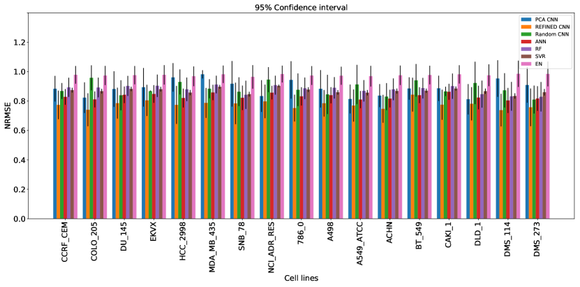
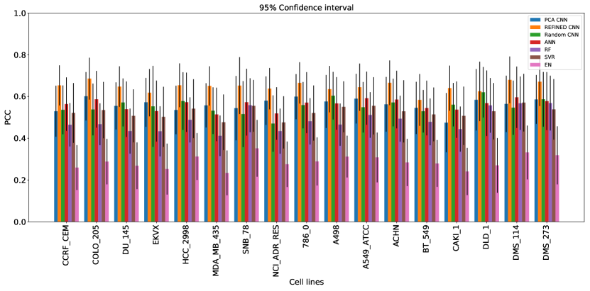
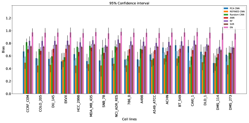
	CCRF_CEM		EKVX		MDA_MB_435		NCI_ADR_RES		SNB_78
Training size	NRMSE	PCC	NRMSE	PCC	NRMSE	PCC	NRMSE	PCC	NRMSE	PCC
20 %	1.279	0.373	0.899	0.4980	0.949	0.454	0.953	0.464	0.876	0.537
40 %	0.985	0.478	0.881	0.511	0.911	0.494	0.958	0.536	0.825	0.590
60 %	0.903	0.538	0.849	0.525	0.839	0.575	0.857	0.528	0.806	0.591
80 %	0.774	0.653	0.804	0.618	0.787	0.651	0.798	0.638	0.784	0.652

Figure 23: First row: Images created using different dimensionality reduction techniques. Second row: Images created using REFINED initialized with different dimensionality reduction techniques. Corresponding NSC = 1

Figure 24: First row: Images created using different dimensionality reduction techniques. Second row: Images created using REFINED initialized with different dimensionality reduction techniques. Corresponding NSC = 171

Figure 25: First row: Images created using different dimensionality reduction techniques. Second row: Images created using REFINED initialized with different dimensionality reduction techniques. Corresponding NSC = 377

Figure 26: First row: Images created using different dimensionality reduction techniques. Second row: Images created using REFINED initialized with different dimensionality reduction techniques. Corresponding NSC = 740

Figure 27: First row: Images created using different dimensionality reduction techniques. Second row: Images created using REFINED initialized with different dimensionality reduction techniques. Corresponding NSC = 5554

Table 14: Results of training CNN on the images created from NCI60 dataset using different dimensionality reduction techniques explained in the Ablation study.

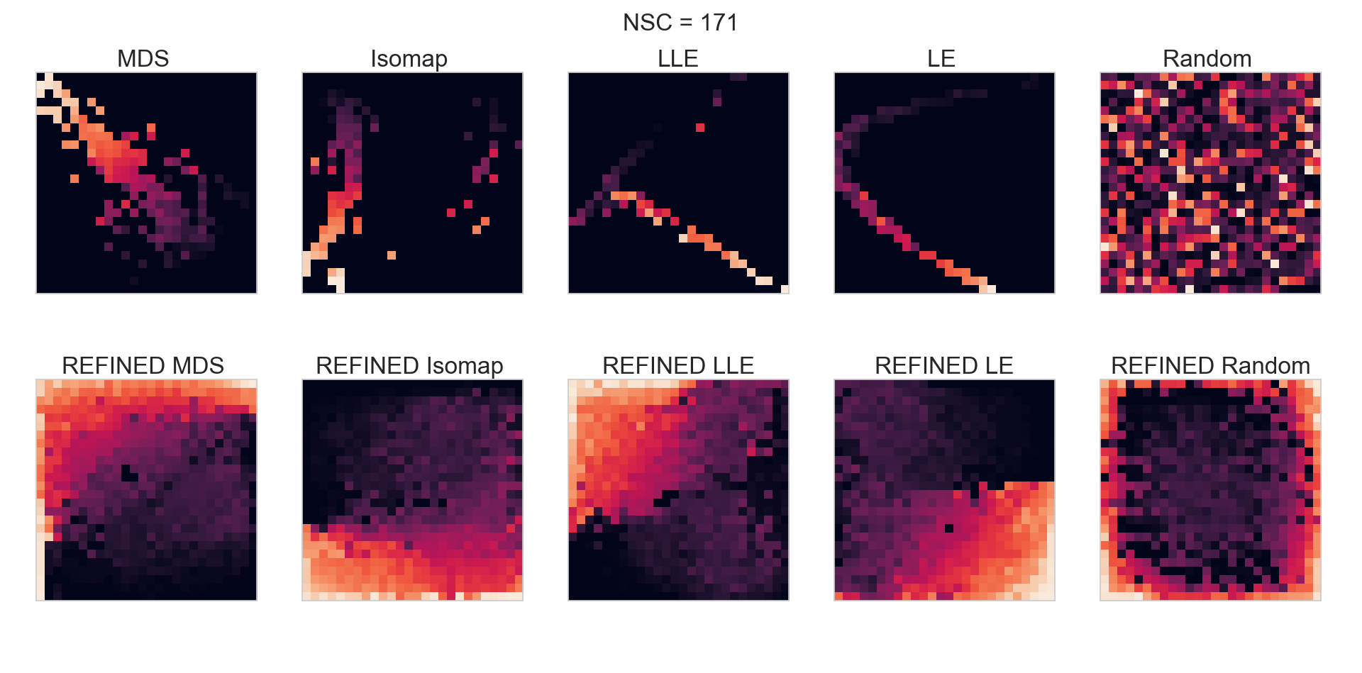
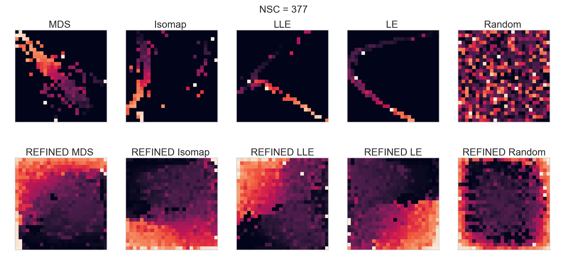
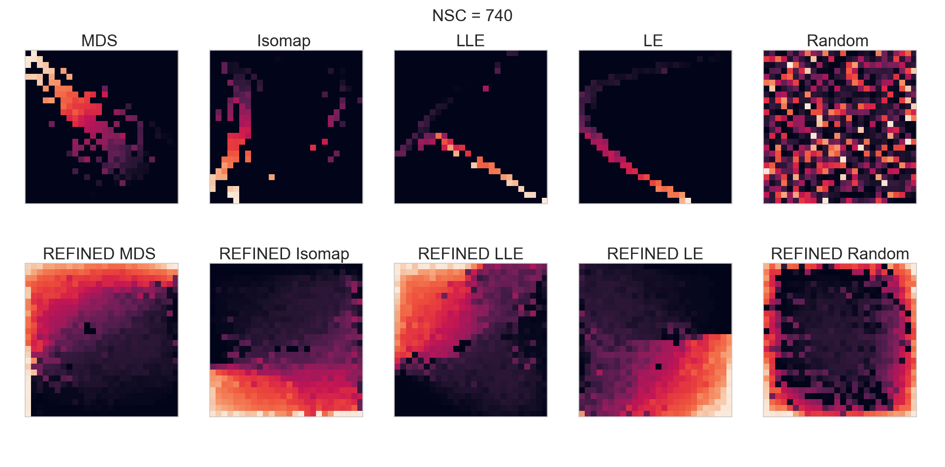
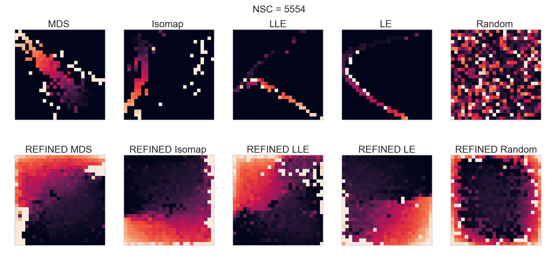
Cell line	Isomap			LLE			MDS			LE			Random
	NRMSE	PCC	Bias	NRMSE	PCC	Bias	NRMSE	PCC	Bias	NRMSE	PCC	Bias	NRMSE	PCC	Bias
CCRF_CEM	0.962	0.470	0.701	0.980	0.233	0.963	0.831	0.622	0.667	0.797	0.614	0.561	0.868	0.536	0.818
COLO_205	0.891	0.584	0.514	1.262	0.000	1.000	0.787	0.622	0.59	0.785	0.641	0.483	0.958	0.538	0.709
DU_145	0.868	0.507	0.724	0.979	0.406	0.835	0.864	0.592	0.523	0.806	0.614	0.533	0.839	0.572	0.594
EKVX	0.853	0.572	0.665	1.021	0.397	0.812	0.867	0.545	0.587	0.841	0.570	0.574	0.867	0.553	0.579
HCC_2998	0.830	0.565	0.630	0.832	0.591	0.562	0.825	0.628	0.467	0.929	0.550	0.545	0.93	0.578	0.744
MDA_MB_435	0.911	0.453	0.773	0.922	0.499	0.643	1.019	0.429	0.748	0.821	0.586	0.632	0.884	0.532	0.76
SNB_78	0.828	0.576	0.598	0.859	0.519	0.754	0.819	0.588	0.684	0.817	0.585	0.684	0.864	0.516	0.73
NCI_ADR_RES	1.315	0.470	0.481	0.895	0.474	0.793	0.938	0.488	0.746	0.824	0.576	0.616	0.945	0.47	0.751
786_0	0.820	0.602	0.546	0.827	0.574	0.677	0.814	0.647	0.66	0.852	0.618	0.477	0.877	0.558	0.604
A498	0.892	0.573	0.534	1.018	0.045	0.998	0.844	0.582	0.681	0.797	0.618	0.537	0.845	0.604	0.712
A549_ATCC	0.801	0.614	0.557	0.851	0.559	0.724	0.896	0.599	0.765	0.825	0.631	0.470	0.913	0.548	0.56
ACHN	1.109	0.494	0.602	0.914	0.462	0.815	0.789	0.631	0.514	0.900	0.601	0.449	0.83	0.571	0.616
BT_549	0.850	0.530	0.701	0.890	0.465	0.768	0.926	0.499	0.764	0.835	0.562	0.624	0.941	0.529	0.595
CAKI_1	0.874	0.548	0.649	1.439	0.376	0.781	0.935	0.546	0.546	0.799	0.609	0.569	0.866	0.561	0.589
DLD_1	0.880	0.587	0.531	0.902	0.468	0.829	0.786	0.629	0.533	0.792	0.636	0.652	0.923	0.62	0.611
DMS_114	0.830	0.577	0.599	0.854	0.539	0.709	0.847	0.619	0.467	0.898	0.602	0.503	0.873	0.546	0.575
DMS_273	0.780	0.639	0.529	0.813	0.598	0.588	0.801	0.62	0.52	0.771	0.639	0.579	0.81	0.587	0.652
Average	0.900	0.551	0.608	0.956	0.424	0.780	0.858	0.582	0.616	0.829	0.603	0.558	0.884	0.554	0.659

Table 15: Results of training CNN on the images created from NCI60 dataset using REFINED initialized with different dimensionality reduction techniques explained in the Ablation study.

Cell line	REFINED_Isomap			REFINED_LLE			REFINED_MDS			REFINED_LE			REFINED_Random
	NRMSE	PCC	Bias	NRMSE	PCC	Bias	NRMSE	PCC	Bias	NRMSE	PCC	Bias	NRMSE	PCC	Bias
CCRF_CEM	0.799	0.630	0.498	0.781	0.638	0.515	0.774	0.653	0.493	0.790	0.633	0.510	0.816	0.586	0.725
COLO_205	0.752	0.673	0.493	0.765	0.652	0.509	0.741	0.686	0.448	0.782	0.658	0.433	0.812	0.606	0.662
DU_145	0.858	0.628	0.443	0.825	0.613	0.531	0.786	0.647	0.458	0.822	0.621	0.595	0.935	0.518	0.604
EKVX	0.790	0.634	0.504	0.839	0.587	0.526	0.804	0.618	0.535	0.824	0.601	0.622	0.998	0.528	0.580
HCC_2998	0.758	0.668	0.456	0.834	0.623	0.465	0.774	0.654	0.447	0.772	0.660	0.451	0.833	0.608	0.454
MDA_MB_435	0.817	0.622	0.495	0.893	0.574	0.688	0.787	0.651	0.469	0.824	0.609	0.559	0.811	0.627	0.586
SNB_78	0.827	0.636	0.436	0.831	0.626	0.458	0.784	0.652	0.448	0.755	0.661	0.547	0.846	0.542	0.778
NCI_ADR_RES	0.791	0.632	0.517	0.823	0.603	0.583	0.798	0.638	0.475	0.811	0.608	0.547	0.810	0.542	0.593
786_0	0.751	0.678	0.504	0.763	0.663	0.467	0.752	0.665	0.450	0.756	0.672	0.451	0.784	0.637	0.661
A498	0.799	0.624	0.508	0.785	0.662	0.435	0.785	0.635	0.433	0.789	0.633	0.569	0.787	0.631	0.669
A549_ATCC	0.754	0.673	0.472	0.779	0.650	0.465	0.769	0.645	0.536	0.750	0.675	0.469	0.858	0.556	0.473
ACHN	0.768	0.684	0.526	0.766	0.656	0.503	0.747	0.665	0.560	0.756	0.659	0.530	0.922	0.585	0.551
BT_549	0.812	0.594	0.583	0.821	0.606	0.521	0.843	0.584	0.560	0.801	0.609	0.585	0.822	0.591	0.708
CAKI_1	0.785	0.639	0.491	0.817	0.590	0.608	0.775	0.640	0.423	0.816	0.617	0.510	0.836	0.571	0.666
DLD_1	0.729	0.687	0.506	0.821	0.622	0.527	0.781	0.625	0.499	0.750	0.680	0.433	0.832	0.594	0.537
DMS_114	0.764	0.671	0.510	0.736	0.690	0.431	0.738	0.680	0.484	0.749	0.676	0.467	0.857	0.563	0.576
DMS_273	0.754	0.667	0.492	0.752	0.693	0.478	0.758	0.670	0.454	0.722	0.701	0.453	0.866	0.546	0.463
Average	0.783	0.649	0.496	0.802	0.632	0.512	0.776	0.647	0.481	0.781	0.645	0.514	0.849	0.578	0.605

Appendix C GDSC dataset

Figure 28: Scatter plot of predicted NLOGIC50s and their residual (error) for each model, in the case where models were trained on 50 % of the available data

Figure 29: Scatter plot of predicted NLOGIC50s and their residual (error) for each model, in the case where models were trained on 20 % of the available data

Table 16: Robustness analysis to compare REFINED CNN with 8 other competing models per each metric. Each cell of the table represents that in what percentage REFINED CNN outperforms the paired competing model.

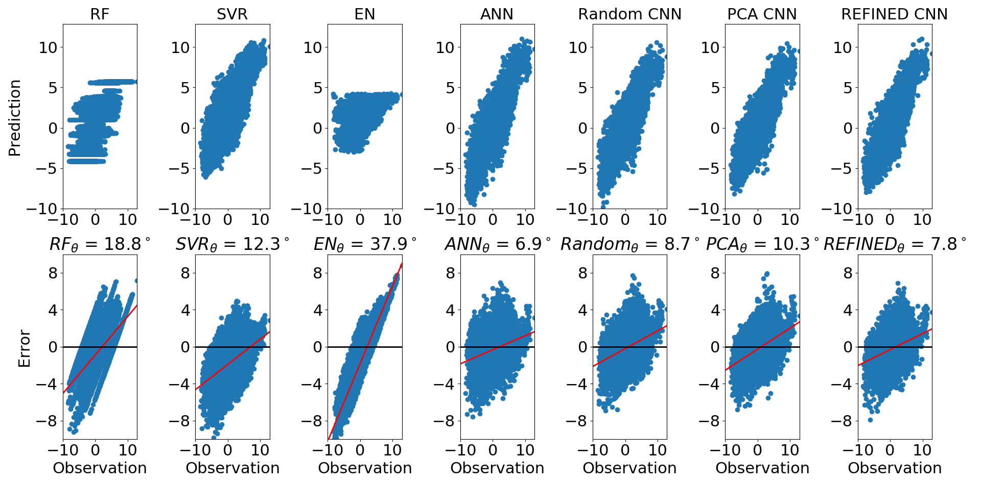
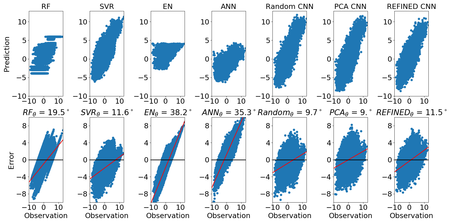
Comparison	NRMSE	PCC	Bias
REFINED CNN vs ANN	62.23	60.68	73.49
REFINED CNN vs RF	98.39	98.19	97.95
REFINED CNN vs SVR	93.83	93.36	73.47
REFINED CNN vs EN	100	100	100
REFINED CNN vs PCA CNN	66.58	62.04	68.85
REFINED CNN vs Random CNN	65.78	69.77	65.27
REFINED CNN vs DRF	100	100	100
REFINED CNN vs HGNN	99.87	98.81	99.99

Table 17: Gap statistics analysis to compare REFINED CNN with 8 other competing models per each metric paired with the null model. The wider (larger) Gap value indicates better performance.

Model	NRMSE	PCC	Bias
REFINED CNN	1.010	0.902	0.853
PCA CNN	0.980	0.892	0.871
Random CNN	0.983	0.895	0.828
RF	0.852	0.812	0.710
SVR	0.898	0.844	0.808
ANN	0.988	0.893	0.815
EN	0.535	0.476	0.200
DRF	0.432	0.184	0.120
HGNN	0.782	0.792	0.550

Figure 30: Distribution of NRMSEs of all nine models drawn from the Gap statistics test of the GDSC dataset. The distributions clustered into two groups and their associated cluster centroids are shown with a vertical bar on the histogram plots.

Figure 31: Distribution of PCCs of all nine models drawn from the Gap statistics test of the GDSC dataset. The distributions clustered into two groups and their associated cluster centroids are shown with a vertical bar on the histogram plots.

Figure 32: Distribution of Biases of all nine models drawn from the Gap statistics test of the GDSC dataset. The distributions clustered into two groups and their associated cluster centroids are shown with a vertical bar on the histogram plots.

Figure 33: Modeling GDSC dataset using different number of genes.

Table 18: Detailed results of modeling GDSC dataset using different number of genes.

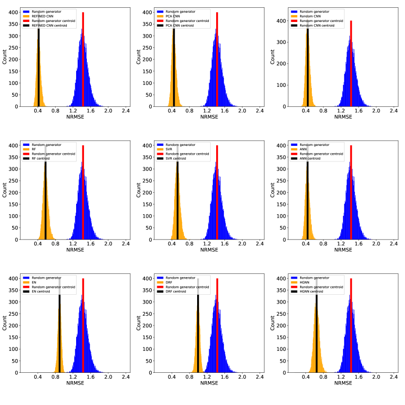
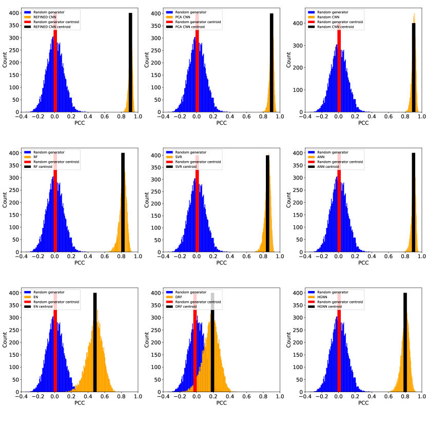
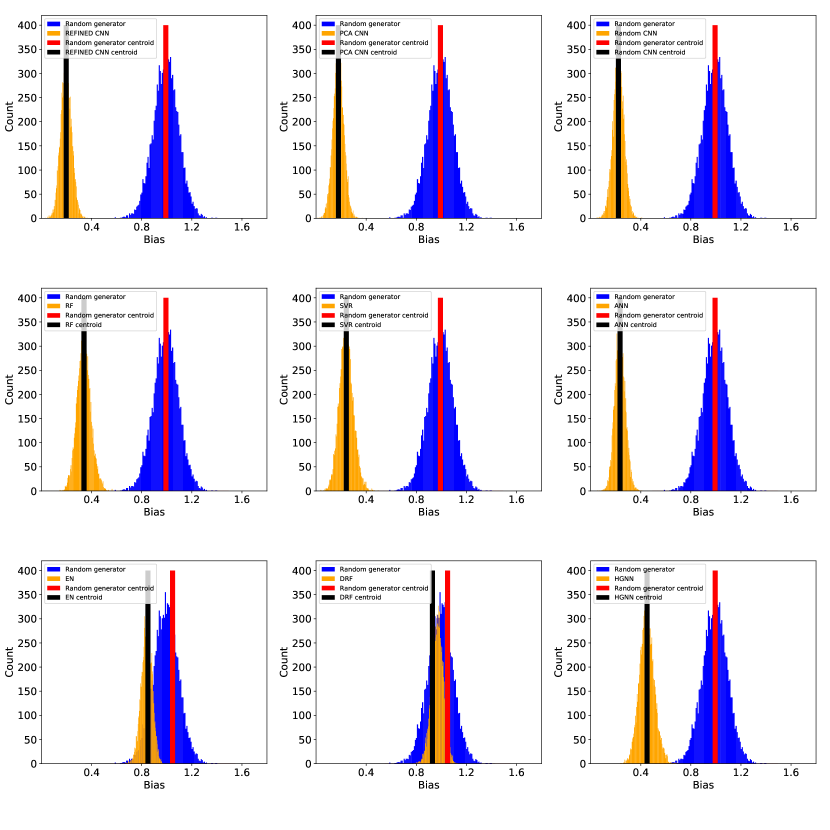
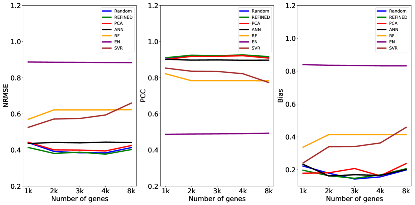
Metrics	1k Genes			2k Genes			3k Genes			4k Genes			8k Genes
	NRMSE	PCC	Bias	NRMSE	PCC	Bias	NRMSE	PCC	Bias	NRMSE	PCC	Bias	NRMSE	PCC	Bias
EN	0.887	0.487	0.840	0.886	0.488	0.836	0.885	0.490	0.835	0.884	0.491	0.833	0.883	0.493	0.833
RF	0.570	0.822	0.337	0.622	0.784	0.414	0.622	0.784	0.414	0.622	0.784	0.414	0.623	0.783	0.414
SVR	0.525	0.854	0.241	0.572	0.836	0.340	0.574	0.835	0.341	0.594	0.822	0.363	0.660	0.774	0.458
ANN	0.436	0.902	0.233	0.442	0.898	0.162	0.440	0.899	0.169	0.444	0.897	0.166	0.441	0.898	0.201
Random CNN	0.441	0.903	0.222	0.392	0.921	0.179	0.385	0.923	0.143	0.384	0.924	0.156	0.413	0.911	0.198
PCA CNN	0.443	0.901	0.179	0.401	0.918	0.181	0.400	0.918	0.207	0.395	0.922	0.163	0.425	0.909	0.237
REFINED CNN	0.414	0.911	0.197	0.381	0.925	0.163	0.388	0.922	0.148	0.377	0.927	0.169	0.402	0.917	0.206

Figure 34: NRMSE with 95 % confidence interval of each model trained on GDSC dataset.

Figure 35: PCC with 95 % confidence interval of each model trained on GDSC dataset.

Figure 36: Bias with 95 % confidence interval of each model trained on GDSC dataset

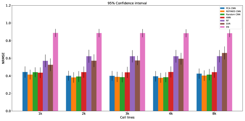
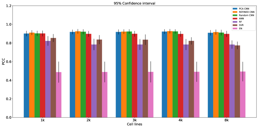
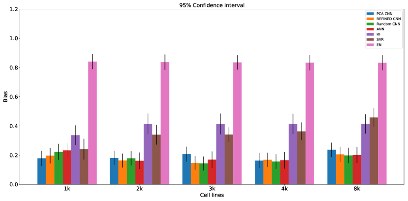
Appendix D REFINED CNN architectures

Figure 37: The architecture of the CNN models used to train the NCI60 dataset (left model is the CNN regressor, right model is the CNN classifier). Plot created by ’graphviz’ utility of keras [55].

Figure 38: The architecture of the CNN model used to train the GDSC dataset. Plot created by ’graphviz’ utility of keras [55].

References

- [1] J. C. Costello and et al. A community effort to assess and improve drug sensitivity prediction algorithms Nature biotechnology, 32, (12), 1202, 2014.
- [2] Q. Wan and R. Pal. An ensemble based top performing approach for NCI-DREAM drug sensitivity prediction challenge PLOS One, 9, (6), e101183, 2014
- [3] Rahman, Raziur and Matlock, Kevin and Ghosh, Souparno and Pal, Ranadip. Heterogeneity aware random forest for drug sensitivity prediction Scientific Reports, 7, (1), 11347, 2017.
- [4] Rahman, Raziur and Otridge, John and Pal, Ranadip. IntegratedMRF: random forest-based framework for integrating prediction from different data types Bioinformatics, 33, (9) , 1407:1410, 2017.
- [5] LeCun, Yann and Bengio, Yoshua and Hinton, Geoffrey. Deep learning nature, 521 (7553), 436, 2015.
- [6] Angermueller, Christof and Pärnamaa, Tanel and Parts, Leopold and Stegle, Oliver. Deep learning for computational biology Molecular systems biology, 12, (7), 878, 2016.
- [7] Wainberg, Michael and Merico, Daniele and Delong, Andrew and Frey, Brendan J. Deep learning in biomedicine Nature biotechnology, 36 (9) : 829, 2018.
- [8] Bengio, Yoshua. Practical recommendations for gradient-based training of deep architectures Neural networks: Tricks of the trade, Springer, 437:478, 2012.
- [9] Iandola, Forrest N and Han, Song and Moskewicz, Matthew W and Ashraf, Khalid and Dally, William J and Keutzer, Kurt. Squeezenet: Alexnet-level accuracy with 50x fewer parameters and¡ 0.5 mb model size arXiv preprint arXiv:1602.07360, 2016.
- [10] Xu, Bowen and Ye, Deheng and Xing, Zhenchang and Xia, Xin and Chen, Guibin and Li, Shanping. Predicting semantically linkable knowledge in developer online forums via convolutional neural network. Proceedings of the 31st IEEE/ACM International Conference on Automated Software Engineering, 51–62, 2016.
- [11] Alipanahi, Babak and Delong, Andrew and Weirauch, Matthew T and Frey, Brendan J. Predicting the sequence specificities of DNA-and RNA-binding proteins by deep learning Nature biotechnology, 33 (8), 831, 2015.
- [12] Coudray, Nicolas and Moreira, Andre L and Sakellaropoulos, Theodore and Fenyo, David and Razavian, Narges and Tsirigos, Aristotelis. Classification and mutation prediction from non-small cell lung cancer histopathology images using deep learning Nature medicine, 24, (10), 1559, 2018.
- [13] Ma, Shiyong and Zhang, Zhen. OmicsMapNet: Transforming omics data to take advantage of Deep Convolutional Neural Network for discovery arXiv preprint arXiv:1804.05283, 2018.
- [14] Shneiderman, Ben Tree visualization with tree-maps: A 2-d space-filling approach Transactions on Graphics11 (1):92–99, 1998
- [15] Ruff, Lukas and Görnitz, Nico and Deecke, Lucas and Siddiqui, Shoaib Ahmed and Vandermeulen, Robert and Binder, Alexander and Müller, Emmanuel and Kloft, Marius. Deep one-class classification. International Conference on Machine Learning, 4390:4399, 2018.
- [16] Esteva, Andre and Robicquet, Alexandre and Ramsundar, Bharath and Kuleshov, Volodymyr and DePristo, Mark and Chou, Katherine and Cui, Claire and Corrado, Greg and Thrun, Sebastian and Dean, Jeff. A guide to deep learning in healthcare Nature medicine, 25, (1), 24, 2019.
- [17] Matlock, Kevin and De Niz, Carlos and Rahman, Raziur and Ghosh, Souparno and Pal, Ranadip. Investigation of model stacking for drug sensitivity prediction BMC bioinformatics, 19, (3), 71, 2018.
- [18] Chang, Yoosup and et al. Cancer Drug Response Profile scan (CDRscan): A Deep Learning Model That Predicts Drug Effectiveness from Cancer Genomic Signature. Scientific reports, 8,(1), 8857, 2018.
- [19] Chiu, Yu-Chiao and et al. Predicting drug response of tumors from integrated genomic profiles by deep neural networks BMC medical genomics, 12 , (1), 18, 2019.
- [20] Davison, Mark Leonard. Multidimensional scaling Wiley New York, (85), 1983.
- [21] Urpa, Lea M and Anders, Simon Focused multidimensional scaling: interactive visualization for exploration of high-dimensional data BMC bioinformatics, 20, (1), 221, 2019
- [22] Shoemaker, Robert H. The NCI60 human tumour cell line anticancer drug screen Nature Reviews Cancer, 6 (10):813,2006.
- [23] Yap, Chun Wei. PaDEL-descriptor: An open source software to calculate molecular descriptors and fingerprints Journal of computational chemistry, 32, (7) , 1466:1474, 2011.
- [24] Yang and et al.. Genomics of Drug Sensitivity in Cancer (GDSC): a resource for therapeutic biomarker discovery in cancer cells Nucleic acids research, 41, (1), 955:961, 2012.
- [25] Barretina, Jordi and Caponigro, Giordano and Stransky, Nicolas and Venkatesan, Kavitha and Margolin, Adam A and Kim, Sungjoon and Wilson, Christopher J and Lehár, Joseph and Kryukov, Gregory V and Sonkin, Dmitriy and others The Cancer Cell Line Encyclopedia enables predictive modelling of anticancer drug sensitivity
- [26] Wold, Svante and Esbensen, Kim and Geladi, Paul Principal component analysis Chemometrics and intelligent laboratory systems, 2, (1-3),37–52, 1987, Elsevier
- [27] Pal, Ranadip. Predictive modeling of drug sensitivity. Elsevier Inc., 2016. 342 p
- [28] Kira, Kenji and Rendell, Larry A. The Feature Selection Problem: Traditional Methods and a New Algorithm. Proceedings of the Tenth National Conference on Artificial Intelligence, AAAI Press, 129–134, 6, 1992.
- [29] Zhang, Guoyi and Lu, Yan. Bias-corrected random forests in regression Journal of Applied Statistics, 39, (1), 151:160, 2012.
- [30] Smouse, Peter E and Long, Jeffrey C and Sokal, Robert R. Multiple regression and correlation extensions of the Mantel test of matrix correspondence. Systematic zoology, 35, (4), 627:632, 1986.
- [31] Efron, Bradley. Bootstrap methods: another look at the jackknife Breakthroughs in statistics, Springer, 569–593, 1992
- [32] Chen, Kun and Chen, Kehui and Müller, Hans-Georg and Wang, Jane-Ling. Stringing high-dimensional data for functional analysis Journal of the American Statistical Association, Taylor & Francis, 106, (493), 275–284, 2011.
- [33] Oh, Man-Suk and Raftery, Adrian E Bayesian multidimensional scaling and choice of dimension Journal of the American Statistical Association, Taylor & Francis, 96, (455), 1031–1044, 2001.
- [34] MacNab, Ying C and Dean, CB. Autoregressive spatial smoothing and temporal spline smoothing for mapping rates, Biometrics, Wiley Online Library, 57, (3), 949–956, 2001.
- [35] Illian, Janine and Penttinen, Antti and Stoyan, Helga and Stoyan, Dietrich. Statistical analysis and modelling of spatial point patterns John Wiley & Sons, 70, 2008.
- [36] Chawla, Nitesh V and Bowyer, Kevin W and Hall, Lawrence O and Kegelmeyer, W Philip. SMOTE: synthetic minority over-sampling technique Journal of Artificial Intelligence Research, 16, 321–357, 2002.
- [37] Ghosh, Souparno and Gelfand, Alan E and Zhu, Kai and Clark, James S. The k-ZIG: flexible modeling for zero-inflated counts, Biometrics, Wiley Online Library, 68, (3), 878–885, 2012.
- [38] Chandler, Richard B and Royle, J Andrew and others. Spatially explicit models for inference about density in unmarked or partially marked populations The Annals of Applied Statistics,,7, 2, 936–954, 2013.
- [39] Ghosh, Sujit K and Mukhopadhyay, Pabak and Lu, Jye-Chyi JC. Bayesian analysis of zero-inflated regression models Journal of Statistical planning and Inference, Elsevier, 136, (4), 1360–1375, 2006.
- [40] Dietterich, Thomas G Approximate statistical tests for comparing supervised classification learning algorithms Neural computation, MIT Press, 10, (7), 1895–1923, 1998.
- [41] Tibshirani, Robert and Walther, Guenther and Hastie, Trevor. Estimating the number of clusters in a data set via the gap statistic Journal of the Royal Statistical Society: Series B (Statistical Methodology), 63, 2, 411–423, 2001
- [42] Witten, Ian H and Frank, Eibe and Hall, Mark A. Practical machine learning tools and techniques Morgan Kaufmann, 578, 2005.
- [43] Vollset, Stein Emil Confidence intervals for a binomial proportion Statistics in medicine, 12, 9, 809–824, 1993.
- [44] Tenenbaum, Joshua B and De Silva, Vin and Langford, John C A global geometric framework for nonlinear dimensionality reduction science, American Association for the Advancement of Science, 290, (5500), 2319–2323, 2000.
- [45] Roweis, Sam T and Saul, Lawrence K Nonlinear dimensionality reduction by locally linear embedding science, American Association for the Advancement of Science, 290, (5500), 2323–2326, 2000.
- [46] Belkin, Mikhail and Niyogi, Partha Laplacian eigenmaps for dimensionality reduction and data representation Neural computation, MIT Press, 15, (6), 1373–1396, 2003.
- [47] Bengio, Yoshua and Paiement, Jean-françcois and Vincent, Pascal and Delalleau, Olivier and Roux, Nicolas L and Ouimet, Marie Out-of-sample extensions for lle, isomap, mds, eigenmaps, and spectral clustering Advances in neural information processing systems, 177–184, 2004.
- [48] Su, Ran and Liu, Xinyi and Wei, Leyi and Zou, Quan Deep-Resp-Forest: A deep forest model to predict anti-cancer drug response Elsevier, Methods, 166, 91–102, 2019.
- [49] Zhang, Chuxu and Song, Dongjin and Huang, Chao and Swami, Ananthram and Chawla, Nitesh V Heterogeneous graph neural network Proceedings of the 25th ACM SIGKDD International Conference on Knowledge Discovery & Data Mining, 793–803, 2019.
- [50] Lim, Jaechang and Ryu, Seongok and Park, Kyubyong and Choe, Yo Joong and Ham, Jiyeon and Kim, Woo Youn. Predicting Drug–Target Interaction Using a Novel Graph Neural Network with 3D Structure-Embedded Graph Representation ACS Publications, Journal of chemical information and modeling, 59, 9, 3981–3988, 2019.
- [51] Cawley, Gavin C and Talbot, Nicola LC. On over-fitting in model selection and subsequent selection bias in performance evaluation Journal of Machine Learning Research 11, July, 2079–2107, 2010.
- [52] Pedregosa, F. and Varoquaux, G. and Gramfort, A. and Michel, V. and Thirion, B. and Grisel, O. and Blondel, M. and Prettenhofer, P. and Weiss, R. and Dubourg, V. and Vanderplas, J. and Passos, A. and Cournapeau, D. and Brucher, M. and Perrot, M. and Duchesnay, E. Scikit-learn: Machine Learning in Python Journal of Machine Learning Research, 12, 2825–2830, 2011.
- [53] Glorot, Xavier and Bordes, Antoine and Bengio, Yoshua. Deep sparse rectifier neural networks Proceedings of the fourteenth international conference on artificial intelligence and statistics, 315–323, 2011.
- [54] Ioffe, Sergey and Szegedy, Christian. Batch normalization: Accelerating deep network training by reducing internal covariate shift arXiv preprint arXiv:1502.03167, 2015
- [55] Chollet, François and others. Keras https://keras.io, 2015