Causal structure based root cause analysis of outliers
Abstract
We describe a formal approach to identify ‘root causes’ of outliers observed in variables in a scenario where the causal relation between the variables is a known directed acyclic graph (DAG). To this end, we first introduce a systematic way to define outlier scores. Further, we introduce the concept of ‘conditional outlier score’ which measures whether a value of some variable is unexpected given the value of its parents in the DAG, if one were to assume that the causal structure and the corresponding conditional distributions are also valid for the anomaly. Finally, we quantify to what extent the high outlier score of some target variable can be attributed to outliers of its ancestors. This quantification is defined via Shapley values from cooperative game theory.
1 Introduction
Although asking for ‘the root cause’ of an unexpected event seems to be at the heart of the human way of ‘understanding’ the world, there is no obvious way to make sense of the concept of a ‘root cause’ using current formalizations of causality like Causal Bayesian Networks (CBNs) [1, 2]. To elaborate on the kind of causal information provided by CBNs, we first recall the causal Markov condition. If the variables are causally connected by the DAG , then their joint distribution factorizes according to
where each denotes the conditional distribution of each , given its parent variables . Whenever has a density with respect to a product measure, the joint density decomposes into [3]
| (1) |
Given that the variable attained some ‘extreme’ value , there is no straightforward answer to the question ‘why did this happen?’. After all, only describes the conditional probability for this event, given the values attained by the parents . At the same time, it also describes the interventional probability of , given that are set to the values .
More detailed causal information is provided if the causal DAG not only comes with a joint distribution but also with a functional causal models (FCMs) [1], also called ‘structural equation models’. There, each variable is given by a function of its parents and an unobserved noise variable
| (2) |
where the noise variables are jointly statistically independent. (2) is said to be an FCM for the conditional if has the distribution for -almost all . FCMs also answer counterfactual questions referring to what would have happened for that particular observation , given one had intervened on and set them to instead of . FCMs are therefore particularly helpful for understanding what happened for that particular event rather than just providing statistical statements over the entire sample.
Here we focus on events that particularly require an ‘explanation’ because they are rare events. Such events can be values or combinations that belong to an a priori defined class of events having low probability. Such events are also called ‘anomalies’ or ‘outliers’ or also ‘extreme events’ (for the special case where values are exceptionally large or small). Outlier detection is a field of growing interest [4, 5] particularly in the context of understanding complex systems like global climate [6], monitoring of cloud computing networks, health monitoring, and fraud detection, just to name a few. The goal of this paper is not to provide yet another tool for outlier detection. Instead, it discusses an approach to infer root causes of outlier events given that the outlier detection problem has been solved and that the causal DAG is available. Here, the causal DAG is assumed not to only describe causal relations in the ‘normal’ regime, but also in the case of the anomalies under consideration.
The paper is structured as follows. Section 2 tries to introduce a systematic quantification of outliers and introduces the class of ‘information theoretic’ outlier scores. Section 3 motivates why this class is particularly helpful for studying causal relations between outliers. Section 4 introduces the concept of conditional outliers as crucial basis for root cause analysis. Section 5 describes how to attribute outliers of some target variable of interest to each single ancestor node. Section 6 describes experiments with real and simulated data.
2 Information theoretic outlier scores
This section introduces some terminology and tools. Although they are not really standard, we do not claim substantial novelty for the major part.
Definition 1 (information theoretic scores).
Let be a random variable with values in and distribution . An information theoretic (IT) outlier score is a measurable function such that
| (3) | |||||
| for -almost all | (4) |
is called surjective if the function is surjective and thus equality holds in (3).
We will often drop random variables as indices in whenever it is clear from the context to which variable we refer to.
For the following reason surjective scores are particularly convenient (but they cannot exist for purely discrete probability space):
Lemma 1 (distribution of surjective scores).
For any surjective , the distribution of on has the density .
Proof.
If is surjective (4) holds for every and thus the cumulative distribution function reads . Its derivative is . ∎
The fact that the probability decays exponentially with increasing score will be convenient later because it ensures that scores behaves almost additive for independent events. It turns out that IT scores are just generalized log quantiles:
Lemma 2 (function-based representation).
Every information theoretic outlier score is of the following form. If is a measurable function, let be defined by
where denotes an arbitrary value attained by .
Proof.
Set . Using property (4) we have and hence . ∎
Example 1 (Rarity).
Let have the density . Setting yields the Rarity
Example 2 (usual log quantiles).
For any real-valued set . Then we obtain the right-sided quantile
For we obtain the left-sided quantile
and for we obtain
The following concept describes a way to generate an outlier score from a set of scores:
Definition 2 (scores from convolution).
For any probability distribution on and two functions and , we call
the convolution score of and . Similarly, we define the convolution for components.
For the special case where and are information theoretic scores, we call the resulting score the convolution of the scores and :
Example 3 (Rarity with product densities).
For two random variables we define and . Let and be independent and have the joint density . Then the rarity
is the convolution score of and with , but not the convolution score of the separate rarities of and . The latter would be given by the function , that is the sum of the logarithms of cumulative tail distributions and not the sum of log densities.
Theorem 1 (multiple convolution).
Let be a product distribution on . Let be surjective information theoretic outlier scores. Then
The proof is in the appendix. Note that this result can be used to define an outlier score for product spaces (given that the components are independent).
For we obtain the concise form
There is a good reason why the resulting score is not the sum of the outlier scores for the subsystems: otherwise the outlier score of a system that consists of multiple components would always be high. The additional term is thus comparable to a correction term for multi-hypothesis testing. After all, each can be seen as the log -value of a statistical test. To understand the relevance of convolution, note that may attain a high value either because at least one of the has been extremely high or because many are higher than expected. To be able to account for both types of exceptional events seems to be an advantage of convolution, compared to more ’pragmatic’ approaches where one just increases the threshold above which one considers an observation an outlier whenever a large set of metrics is taken into account.
There are certainly a broad variety of possible definition of outlier scores. A very simple example would be, for instance, the normalized distance from the mean: if is real-valued, just define the z-score
| (5) |
Then Chebyshev’s inequality also guarantees, to some extent, that high outlier scores are rare due to , although the probability doesn’t decay exponentially. However, for fixed unimodal distributions like Gaussians the z-score can be easily translated into the IT score Example 2 (or equivalently Example 1) via the non-linear monotonic transformation
The following two sections suggest that information theoretic scores are particularly useful for discussing conceptual problems of root cause analysis – even if z-score is often convenient because it avoids statistical problems of estimating cumulative distributions.
3 Can a weak outlier cause a stronger one?
In complex systems, outliers will certainly cause each other because, for instance, unexpectedly large values of one quantity may yield unexpectedly large values for quantities influenced by the former one. Within such a cascade of outliers one may want to identify the ‘root cause’ – after first defining what this means. It is tempting to consider the strongest outlier as the root cause. If the causal structure between the variables is known (in terms of a causal Bayesian network [1], for instance), one may alternatively search for the ‘most upstream’ node(s) among those whose outlier scores are above a certain threshold, but since it is not clear where to set the threshold we will not discuss this any further. To motivate a more principled approach to root cause analysis, let us first describe how choosing the largest outlier as root cause may fail.
Example with ‘bad’ outlier score
Let us first consider problems with z-score (5) applied to non-Gaussian variables. Assume two variables are linked by the simple causal structure and the (deterministic) structural equation reads . Assume symmetric distributions with . Then we have and . Hence,
This shows that large outliers cause a considerably even stronger outlier downstream, but here this is the result of that particular definition of the outlier scores.
Example with IT outlier score
Let and be Gaussian variables and influence via the linear structural equation
where and is an independent noise with . Recall that the z-score now is an IT score up to monotonic reparameteriation. Let us set manually to the value , which is already a strong perturbation (values deviating from the mean by standard deviations or more occur with probability less than ). Assume further that attains the value , which results in attaining , which is a quite strong outlier because . Hence, is a stronger outlier than in terms of Rarity and Log Quantiles. From an intuitive perspective, however, contributed more to being an outlier than itself. After all, did not behave in an unexpected way, given the high value of its parent ; noise values of the size of the standard deviation are not particularly unlikely ().
There is, however, a sense in which an outlier is unlikely to cause a significantly stronger one with respect to an IT score:
Lemma 3 (relations between outlier scores).
For any we have
for almost all .
Proof.
We have:
where we used that holds for all . ∎
Note that Lemma 3 holds independently of whether is the cause and the effect or vice versa: Plugging an outlier with into any causal mechanism , is unlikely to cause an effect whose outlier score is significantly larger than . On the other hand, given that the effect has outlier score at least, it is unlikely that the cause plugged into the mechanism had an outlier score significantly larger than .
4 Conditional outlier scores
The previous section discussed to what extent the value attained by a node is unexpected given the value of its parents. The intuition behind this question implicitly referred to a notion of conditional outlier scoring, which we now introduce formally by using the the conditional distribution of , given its parents. Defining outlier scores by conditional distributions given some background information is certainly not novel [7]. The present paper, however, emphasizes that analyzing the causal contribution of each node to an outlier requires ‘causal conditionals’, that is, conditionals of a node given its parents. If an anomaly is likely, given its parents, we would consider the anomaly as ‘caused by’ the latter and not caused ‘by the node itself’. In contrast, whether the anomaly is likely given its children, is irrelevant for root cause analysis.
4.1 Two variable case
We first restrict the attention to a causal structure with just two variables where is the cause of . Generalizing this to the case where the target variable is influenced by multiple causes will be straightforward since none of the results requires to be one-dimensional.
Definition 3 (Conditional outlier score).
Let be random variables with range , respectively, and causally linked by . A measurable function is called conditional IT outlier score if for all , is an IT score with respect to the conditional distribution .
It will be convenient to write instead of . The following property supports the view that conditional outliers quantify to what extent an unlikely event happened at the particular node under consideration and not at its parents:
Lemma 4 (independence of surjective scores).
If is a surjective IT score for every , then
The lemma is an immediate consequence of Lemma 1 since has the same density for all .
We have emphasized that conditional outlier score is supposed to measure to what extent something unexpected happened at that particular node. This perspective is facilitated when a conditional outlier score is – a priori – defined by an outlier of the unobserved noise that corresponds to that node in an FCM:
Definition 4 (FCM for conditional score).
A conditional IT outlier score is said to have an FCM if there is an FCM with range for and an IT score such that is a function of and .
Lemma 5 (existence of FCM for a conditional score).
A conditional IT outlier score has an FCM if and only if
The proof is in the appendix.
4.2 Causal Bayesian Network
Since Definition 3 did not put any restriction on the range , we can thus assume to be the multivariate variable that consists of all parents of a variable in a Bayesian network and obtain, in a canonical way, the conditional score
where denotes the range of .
Whenever the outlier scores have an FCM in the sense of Definition 4, they are independent random variables. To decide whether an observed -tuple defines an outlier event, we can then again use the notion of convolution:
Definition 5 (convolution of cond. scores).
Given conditional IT outlier scores for some Bayesian network that are independent as random variables, let be given by
Then the convolution score is defined via
By straightforward adaption of the proof of Lemma 1 we obtain for this case:
Theorem 2 (convolution is subadditive).
Whenever are independent random variables having the density , we have
5 Attributing outliers of a target variable to its ancestors
In applications one may often be interested in outliers of one target variable, say , and wants to attribute this outlier to its ancestor nodes, or more precisely, to quantify to what extent each node contributed to the observed outlier . Assume, without loss of generality, that is a sink node, that is, that it has no descendants and that we are given an FCM of all the variables with noise variables with outlier scores given by for . By recursively applying (2) we can write as deterministic function of all noise variables. Therefore,
| (6) |
The first equality is due to Definition 1 and the second because is a deterministic function of . We can thus change (6) step by step from to by dropping more and more of the components from the vector . It is tempting to quantify the contribution of each node by the change caused by dropping , but this value depends on the ordering of nodes. Fortunately, there is the concept of Shapley values from cooperative game theory that solves the problem of order-dependence by averaging over all possible orderings in which elements are excluded [8].111More recently, Shapley values have also been used in the context of quantifying feature relevance [9]. We rephrase this concept for our context. First, we define the contribution of , given some set not containing , by
We then define the Shapley contribution of by
| (7) |
The following result is a straightforward application of Shapley’s idea and follows because is just defined by symmetrization over all possible orderings.
Theorem 3 (decomposition of target outlier score).
The outlier score of any variable decomposes into the contribution of each of its ancestors:
Note that this contribution can be negative which makes perfectly sense: one value being extreme can certainly weaken the outlier of the target, that is, a more common value at that node would have made the outlier even stronger.
6 Experiments
The goal of the following experiments were to explore whether the concept of conditional outliers is better at finding the root cause of outliers than the naive approach of comparing unconditional outlier scores. The difference between IT scores and other scores did not play a role for these experiments because we work with simple Gaussian probabilistic models to keep the focus on the difference between conditional versus unconditional score. The main purpose of Sections 2 and 3 was to provide a solid basis for outlier scoring in the first place before discussing the difference between conditional versus unconditional scores.
Synthetic Datasets
Here we injected perturbations to randomly chosen nodes in random DAGs. Each node had a chance to be perturbed by a change of the structural equation from
| (8) | ||||
| (9) |
where is a parameter which we refer to as the perturbation strength from here onwards, and is the standard deviation of the noise (by restricting the attention to additive noise models [10] in (8) defines a natural scale to define perturbation strength). We have considered the node(s) at which the perturbation was injected as the ‘root cause(s)’ of the outlier.
We have generated DAGs with nodes (to guarantee sufficient sparsity we have decided to chose parentless nodes and nodes for which the number of parents is randomly chosen with probabilities decaying inverse proportional to ). The function is chosen as follows. (1) With 20% chance, linear with random coefficients in and no intercept. (2) With 80% chance, a random non-linear function generated by a neural network with one hidden layer, random weights in , a random number of neurons in , and the sigmoid activation function. This way, we guarantee to have some linear and, in practice more common, complex non-linear relationships. The noise is chosen Gaussian or uniformly distributed with randomly chosen width.
For each node in the causal graph, we sampled 2000 observations. We inferred a node to be perturbed whenever its unconditional score (this defined the baseline) or its conditional score (our proposal) exceeded some threshold. We used z-score (5) as unconditional score and
| (10) |
as conditional score, where the conditional expectation was estimated via a simple linear regression model. Again, this is a valid conditional IT outlier score with respect to a linear Gaussian probabilistic model. The value is then just the value of the Gaussian noise and the conditional standard deviation is the standard deviation of the noise. To avoid estimating cumulative tail distributions (which requires large sampling) we applied the simple z-score also to our non-Gaussian variables, also to test the robustness of our method with respect to violations of distributional assumptions.
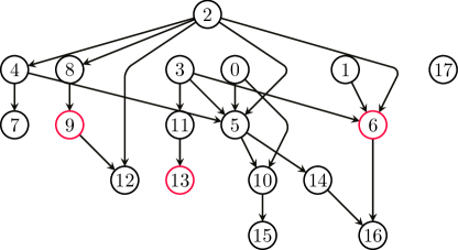
First we examined how perturbation strength affects the performance of outlier scores for a fixed random DAG shown in Figure 1. The nodes marked in red are the root causes of outliers, that is, the perturbed nodes. We estimate the functional relationship between a node and its parents by a random forest with 100 trees and a maximum depth of 7 on the training set. In the test set, we compare ROC curves of both scores at various values of perturbation strength. The results are shown in Figure 6.
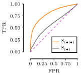
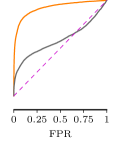
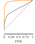
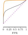
Already at , we observe that conditional outlier score is much better at identifying root causes than its unconditional counterpart. Unlike unconditional outlier score, the true positive rate (TPR) of conditional outlier score shoots up quickly with a slight increase in false positive rate (FPR). As the perturbation strength increases, the conditional outlier score identifies most of the root causes (true positives) only at a rather small cost of allowing very few false positives, in contrast to unconditional outlier score.

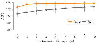
We sampled 190 causal graphs, and report average area under ROC curve (AUC) together with the sample standard deviation at various values of perturbation strength in Figure 8. We see that the results corroborate the findings from our previous experiment. The performance of both scores improve with the increase in the perturbation strength. The conditional outlier score, however, consistently performs better than unconditional outlier score.
Real Dataset
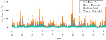
Here we considered daily river flow, measured in cubic metres per second, at various locations along three rivers in England.222https://environment.data.gov.uk/hydrology/explore In particular, we consider the daily river flow at the New Jumbles Rock () measurement station, which is located right after the confluence of rivers Hodder, Calder, and Ribble. Furthermore, we consider three other measurement stations upstream of the confluence: Hodder Place () along River Hodder, and Henthorn () along River Ribble, and Whalley Weir () along River Calder (see Figure 7). As river flow downstream of the confluence is the result of river flows upstream, we can reasonably assume the following causal graph333Note, however, that downstream water levels can in principle also influence upstream ones by slowing down the flow., up to unobserved common causes like weather conditions (e.g. precipitation and temperature), which we haven’t accounted for since this required deeper domain knowledge like time delay of these influences.
![[Uncaptioned image]](/html/1912.02724/assets/x9.png)
For each measurement station, we take daily river flows, measured at 9:00 a.m. every day, from 1 January 2010 till 31 March 2019 (shown in Figure 7). If a daily measurement is missing in one of the stations, we remove the corresponding daily measurements from all other stations. Consequently we end up with 3357 measurements. We use 3267 measurements before 1 January 2019 for fitting the structural equations, and the remaining 90 measurements, from the year 2019, for testing.
Assuming that the underlying data generation process follows a linear additive noise model, we can represent the causal graph above with the structural equations for and
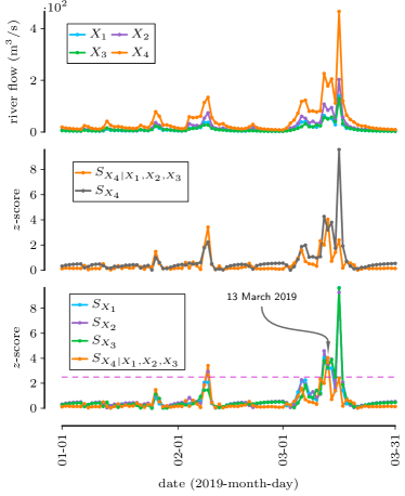
where is the noise variable corresponding to the variable . For the z-scores, we again estimated means and variances of variables , , and . For , we apply ordinary least squares linear regression, and again estimated the mean and the variance of the resulting noise and estimated condional z-score (10). As histograms of noise variables suggest a roughly Gaussian shape, it again suffices to use a simplified outlier score such as the normalized distance from the mean. First we compare conditional against unconditional outlier scores on the test set at the New Jumbles Rock measurement station () in Figure 9 (middle).444Note that conditional and unconditional outlier scores are the same for , , and because they do not have any parents in the causal graph. We observe that unconditional outlier score is not only often larger but also more sensitive to changes than its conditional counterpart. Consider the two scores on 16 March 2019, for instance. On this day, river flow is the largest at the New Jumbles Rock station. This is not surprising, however, given the high volume of water upstream. The conditional outlier score takes that into account, and is hence a mere . The unconditional outlier score, on the other hand, is a massive .
Next we investigate the root cause of outlying measurements. To this end, in Figure 9, we plot conditional outlier scores of measurements on the test set for all nodes in the causal graph. We examine one day in particular here. On 13 March 2019, for instance, we observe that conditional outlier scores of measurements at all the nodes are very high. This suggests us that something unlikely happened in all those nodes on that day before 9:00. One possible explanation is the heavy rainfall early morning in Lancashire county where the rivers are located in.
Overall the experiments show that conditional outlier scores may differ significantly from unconditional ones. Consequently, even simple linear regression models sometimes suffice to explain outliers as resulting from upstream outliers. After all, every event for which large conditional outlier score come with small conditional scores show that the FCM fits well for that particular event. Also our simulation experiments suggest that values that have low conditional outlier score but high unconditional score are just downstream effects. Of course we have no ground truth regarding the ‘root causes’ – it is not even clear how to define it without the concept of conditional outliers introduced here.
7 Discussion
We have proposed a way to quantify to what extent an observation is an unlikely event given the value of its causes in a scenario where the causal structure is known. This way, we can attribute rare events to mechanisms associated with specific nodes in a causal network. This attribution is formally provided by two different main results. First, Theorem 2 relates the outlier score of a collective event to conditional outlier scores of each nodes. Second, Theorem 3 quantitatively attributes the outlier score of one target variable to unexpected behavior of its ancestors. Our results do not solve the hard problem of causal discovery [2], that is, the question of how to obtain the causal DAG in the first place. Instead, it aims at providing a framework to formally talk about attributing rare events to root causes when the causal DAG is given and the structural equations are either given or inferred from data .555Structural equations do not uniquely follow from observed joint distributions even when the DAG is given [1], but they can be inferred subject to appropriate assumptions, e.g., additive noise [10].
To avoid possible misunderstandings, we emphasize that anomalies may certainly occur because the causal DAG, the structural equations, or the corresponding noise distributions do not hold for that particular statistical realization. The fact that our computation of conditional outlier score is based on assuming a fixed DAG, structural equation, and noise distribution does not mean that we exclude these changes. The conditional outlier score should rather be considered as the negative logarithm of a p-value that can be used for rejecting the hypothesis that the given structural assumptions still hold for the given anomalous event.
Acknowledgements: Thanks to Atalanti Mastakouri for comments on an earlier version of the manuscript.
8 Appendix
8.1 Proof of Theorem 1
For surjective outlier scores we can without loss of generality assume with the density , see Lemma 1. Set . The density on as the positive cone of is then given by
We have to integrate this density over the simplex with and thus obtain
| (11) |
We now perform the substitution with with Jacobian determinant and obtain for (11):
The inner integral is just the volume of the simplex in given by and , which reads . We thus obtain
Using [11]
with , , and we obtain
Inserting and taking the logarithm of the probability completes the proof.
8.2 Proof of Lemma 5
The ‘only if’ part is obvious since is by definition of FCMs independent of . To show the converse direction, let be an FCM for for some noise variable . Define a modified FCM
| (12) |
with noise variable , where has the same range as and . Define an outlier score for by
To show that it satisfies the distributional requirements of an IT score we need to show for -almost all . By assumption we have for -almost all . Due to the independence of and the distribution of coincides with the distribution of for -almost all . Thus we have for -almost all , which shows that is an IT score.
Then, define a joint distribution of by
with
We observe that due to weak contraction because by construction and by assumption. Further, has the same distribution as since . Hence, (12) is also an FCM for . Moreover, we have
by construction. Hence we have constructed an FCM for .
References
- [1] J. Pearl. Causality. Cambridge University Press, 2000.
- [2] P. Spirtes, C. Glymour, and R. Scheines. Causation, Prediction, and Search. Springer-Verlag, New York, NY, 1993.
- [3] S. Lauritzen. Graphical Models. Clarendon Press, Oxford, New York, Oxford Statistical Science Series edition, 1996.
- [4] V. Chandola, A. Banerjee, and V. Kumar. Anomaly detection: A survey. ACM Comput. Surv., 41, 07 2009.
- [5] S. Guha, N. Mishra, G. Roy, and O. Schrijvers. Robust random cut forest based anomaly detection on streams. In Proceedings of the 33rd International Conference on International Conference on Machine Learning - Volume 48, ICML’16, pages 2712–2721. JMLR.org, 2016.
- [6] J. Zscheischler, S. Westra, B.. van den Hurk, S. Seneviratne, P. Ward, A. Pitman, A. AghaKouchak, D. Bresch, M. Leonard, T. Wahl, and X. Zhang. Future climate risk from compound events. Nature Climate Change, 8(6):469–477, 2018.
- [7] J. Song, S. Oyama, and M. Kurihara. Tell cause from effect: models and evaluation. International Journal of Data Science and Analytics, 2017.
- [8] L. Shapley. A value for n-person games. Contributions to the Theory of Games (AM-28), 2, 1953.
- [9] A. Datta, S. Sen, and Y. Zick. Algorithmic transparency via quantitative input influence: Theory and experiments with learning systems. In 2016 IEEE Symposium on Security and Privacy (SP), pages 598–617, 2016.
- [10] P. Hoyer, D. Janzing, J. Mooij, J. Peters, and B Schölkopf. Nonlinear causal discovery with additive noise models. In D. Koller, D. Schuurmans, Y. Bengio, and L. Bottou, editors, Proceedings of the conference Neural Information Processing Systems (NIPS) 2008, Vancouver, Canada, 2009. MIT Press.
- [11] I. Bronshtein. A Guide Book to Mathematics. Springer, 1973.