A fractional Brownian - Hawkes model for
the Italian electricity spot market:
estimation and forecasting

Abstract

We propose a model for the description and the forecast of the gross prices of electricity in the liberalized Italian energy market via an additive two-factor model driven by both a Hawkes and a fractional Brownian processes. We discuss the seasonality, the identification of spikes and the estimates of the Hurst coefficient. After the calibration and the validation of the model, we discuss its forecasting performance via a class of adequate evaluation metrics.

1 Mathematical modelling of electricity markets

This paper presents a modelling and computational work, related to the description and forecasting of prices in the Italian wholesale electricity market. We discuss the choice of the particular model, above all the representation of the source of randomness, related to the baseline evolution of prices via a fractional Brownian motion and to the spiky behaviour via a Hawkes process. The computational part of the work regards to problems of parameter estimation and dataset filtering. These are crucial steps in the pre-processing phase of the model. We evaluate the performance of the model by means of the production of forecasts of future electricity prices, at different forecasting horizons with the aim of evaluating more into details the quality of the forecasts in the distributional sense, instead of giving a single prediction value. Adequate metrics are taken into consideration, as the Winkler score and the Pinball loss function.

In the last decades the electricity market has been liberalized in a growing number of countries, especially in the European Union. Liberalized markets have been introduced for example in Germany, Italy, Spain, UK, as well as in all nordic countries. The introduction of competitive markets has been reshaping the landscape of the power sectors. Electricity price now undergoes to market rules, but it is very peculiar. Indeed, electricity is a non-storable commodity, hence the need of having a particular organization in the market emerged. This has usually resulted in the creation of a day-ahead market: a market in which every day there are some auctions regarding the delivery of energy at a fixed time of the following day. The price of the electricity is determined by crossing the supply curve and the demand curve, for the hour for which the auction is taking place (see e.g. [35]). The steepness of supply and demand curve can be regarded as the cause of one of the main characteristics of the electricity price market, i.e. shock formation in the prices, which is one of the most important aspects that distinguish the electricity market from the other similar financial markets, and also one of the most difficult to model. A shock, or spike is a sudden large rise in the price followed by a rapid drop to its regular level.

The distinction between spiky and “standard” behavior turns out to be crucial in the modelling of the electricity price: the need to obtain a good reproduction of the spikes in the models represents one of the main differences between other financial markets and the electricity one. Another important difference with respect to other markets is the seasonality that can be observed. It is mainly due to a clear weekly periodicity, caused by the fluctuations in consumptions during different days of the week [35]. There is also a long-term seasonal effect on the prices, which appears over time lengths of approximately 3-4 months.

There is a widespread mathematical literature about electricity spot market, both for the modelling [3, 4, 5, 6, 7, 9, 16, 17, 24, 36, 26, 27, 28, 39, 38, 37] and the calibration problems [23, 30, 31, 37, 39]. Two of the first models for electricity price are due to Schwartz [36, 26]. In [36] the authors introduced an Ornstein-Uhlenbeck model for the spot price dynamics which included a mean-reversion component, and later on, in [26], a deterministic component describing the seasonality was added. Since this works, a widespread literature has been proposed in order to model the basic features of this market, especially about the formation of spikes, which were not covered by the aforementioned papers [36, 26]. An interesting review of the state of the art has been given by Weron in [39]. The interested reader may also refer to the huge amount of papers therein. Weron proposes a classification of the models in five main classes: i) the multi-agent models, which simulate the operation of a system of heterogeneous agents interacting with each other, and build the price process by matching the demand and supply in the market; ii) the fundamental structural methods, which describe the price dynamics by modelling the impacts of important physical and economic factors on the price of electricity; iii) the reduced-form stochastic models, which characterize the statistical properties of electricity prices over time, with the ultimate objective of derivatives evaluation and risk management; iv) the statistical models, which are either direct applications of the statistical techniques of load forecasting or power market implementations of econometric models; v) the computational intelligence techniques, which combine elements of learning, evolution and fuzziness to create approaches that are capable of adapting to complex dynamic systems.

The model we present here mainly belongs to the class of the reduced-form model: the time evolution of the spot price is described by an additive terms with a drift described by a deterministic function which models the long–term seasonality and two additive noises described as solution of two independent stochastic differential equations. The model has the following form

$$S(t)=f(t)+\sum_{i=1}^{2}X_{i}(t),\quad t\geq t_{0}\in\mathbb{R}_{+},$$

where $f$ is a deterministic function and the $X_{i}$, for $i=1,2$ are two stochastic processes, responsible of the standard fluctuations which give rise to the standard behavior, i.e. the so called base component, and the spiky behavior of the price evolution, respectively. Both of them show a mean reverting property. Different examples of these kind of models may be found for example in [27, 28, 39, 24].

The novelty here is that we consider a fractional Brownian motion as the driving noise of the base component instead of the usual standard Brownian motion. In particular, the process $X_{1}$ is a fractional Ornstein-Uhlenbeck process. The main modelling reason is that among the characteristics of the spot prices, one the presence of self-correlations in the price increments has to taken into account. The presence of this feature suggests, when trying to model these kind of markets, to modify the structure of the existing models to include the self-correlations. One of the possible choices that have been used in literature so far is to consider a fractionally integrated ARFIMA model, a generalisation of the classical ARIMA model, as it has been done in [17], and in other cases reported in the review [39]. In particular, in [17] this has been done for the Italian electricity market. Here we go further than the pure statistical models.

In literature there have been several attempts of using a fractional Brownian motion in financial market modelling, even if not in the case of the electricity one. Its relatively simple nature, combined with its flexibility in modelling data whose increments are self–correlated, gave rise to a growing number of models involving fractional Brownian motion. Anyway, it was pointed out quite early in [34] that a model involving fBm would result in admitting the presence of some kind of arbitrage in the market. More into details, in [11] the author proved that there are strong arbitrage opportunities for the fractional models of the form

$$\begin{split}X(t)=&\nu(t)+\sigma B^{H}(t)\\ X(t)=&\exp(\nu(t)+\sigma B^{H}(t)),\\ \end{split}$$ (1)

where $\nu(t)$ is a measurable bounded deterministic function and $B^{H}$ is a fractional Brownian motion of Hurst parameter $H\in(0,1)$. This arbitrage opportunities can be built provided that we are allowed to use the typical set of admissible trading strategies (see [11] for the complete definitions). This set of admissible strategies in particular allows to buy and sell the stock continuously in time, which is a questionable assumption in many frameworks. In [11] the author proved that for the models (1) the arbitrage opportunities disappear, provided that we restrict the set of strategies to the ones that impose an arbitrary (but fixed) waiting time $h>0$ between a transaction and the following one. We recall that in the present work we consider a fractional Ornstein–Uhlenbeck process. We cannot use directly the results in [11], but the extension to this family of processes should be straightforward and may be subject for future work.

A striking empirical feature of electricity spot prices is the presence of spikes, that can be described by a jump in the price process immediately followed by a fast reversion towards the mean. It is interesting to notice that in the case of the Italian electricity market the presence of several jumps is shown, many of which appearing clustered over short time periods. As a consequence, the second component $X_{2}$ is solution of a mean reverting processes driven by a self-exciting Hawkes process, which is a jump process whose jumps frequency depends upon the previous history of the jump times. In particular, right after a jump has occurred, the probability of observing a subsequent jump is higher than usual. The interested reader may refer to [2, 21] fo an excellent survey on the introduction, the relevant mathematical theory and overview of applications of Hawkes processes in finance and for more recent financial applications.

We conclude the discussion on the model via some simulation results and the problem of estimation of the parameters of both the signals.

The second part of our paper is devoted to a complete computational study. We apply the model to the study case of the time series of the Italian MGP, the data of the day-ahead market (see [40]) from January 1, 2009 to December 31, 2017. The first two years are the sample considered for the estimation and validation of the model. We carry out the difficult task of separating the components of the raw prices into our main components (weekly component, long-term seasonal component, standard behaviour, spiky behaviour). Then we deal with the problem of the estimation the parameters of the model and we test the forecasting performance of our model on forecasting horizons from one to thirty days. The parameters are estimated in a rolling window fashion, as summarized in [31]. We construct prediction intervals (PI) and quantile forecasts (QF) and evaluate them via a class of adequate evaluation metrics like the Winkler score and the Pinball loss function.

We conclude that the analysis shows some quantitative evidence that both the fractional Brownian motion and the Hawkes process are adequate to model the electricity price markets.

The paper is organized as follows. Section 2 is devoted to a brief presentation of both the fractional Brownian motion and the Hawkes processes with their main properties. We perform some numerical simulations for some specific parameters. In Section 3 we discuss the method of estimation of the parameters, by validating the estimates by calculating the 5% and the 95% quantiles. Section 4 is dedicated to the study case. Preliminary analysis and a data filtering process are implemented. A in sample estimation is carried out and then an out od sample forecasting is realized. The section ends with our conclusion.

2 A model driven by a Hawkes and a fractional Brownian processes

The model we propose extends in different ways some relevant models already available in the literature. In particular, we consider a modification of the model proposed in [6, 28] and then modified for example in [24], by including some self–exciting features, via Hawkes-type processes and correlation of the increments via a fractional Brownian motion.

2.1 The equations

We adopt an arithmetic model as in [3, 7, 6, 24] in which the power price dynamics is assumed to be the sum of several factors. We suppose that the spot price process $S=\{S(t),t\in\mathbb{R}_{+}\}$ evolves according to the following dynamics

$$S(t)=f(t)+{X}(t).$$ (2)

The function $f(t)$ describes the deterministic trend of the evolution, while the process ${X}=\{{X}(t),t\in\mathbb{R}_{+}\}$ describes the stochastic part. The latter is a superposition of two factors: $X_{1}$, known in literature as the base component, which is continuous a.e. and aims to model the standard behavior of the electricity price, and $X_{2}$ which is the jump component, describing the spiky behavior of the electricity prices, overlapped to the base signal. This means that, for any $t\in\mathbb{R}_{+}$,

$${X}(t)=X_{1}(t)+X_{2}(t).$$ (3)

The main reason to consider two additive signal driven by the two different noises is relating of our assumption of mean-reversion: despite the possible noise, the price tends to fluctuate around a specific level. In particular, our starting assumption is that both in the base and spiky regimes prices tend to revert towards their own mean, and we presume that the strength of reversion might be different. This is because we expect that whether the price strongly deviates from the mean value, as during a spike, then it returns to the average level with a stronger force than usual.

Regarding the base component, let us note that in many time series of the electricity markets, an evidence of correlation among price increments is clear. For example, see Figure 11. In order to capture better such a correlation within different returns, we consider an additive noise driven by a fractional Brownian motion.

Furthermore, the Italian market is rather peculiar since clearly identifiable spikes are rare; as a consequence the intensity of the spike process is small and becomes difficult to be estimated. Moreover, despite the small number of spikes, a clustering effect seems to be present; so one might better include the effect of a self-exciting stochastic process. Hence, by following recent literature [1, 2, 4, 10, 12, 18, 24], we model the jump component $X_{2}$ via a Hawkes marked process.

To be more precise, let us consider a common filtered probability space $(\Omega,\mathcal{F},\{\mathcal{F}_{t}\}_{t\in\mathbb{R}_{+}},P)$. We suppose that $X_{1}$ follows a stochastic differential equation driven by a fractional Brownian motion $B^{H}=\{B^{H}(t),t\in\mathbb{R}_{+}\}$ with Hurst parameter $H\in(0,1)$ and diffusion coefficient $\sigma\in\mathbb{R}_{+}$, subject to mean reversion around a level zero, with strength $\alpha_{1}\in\mathbb{R}_{+}$.

A Fractional Brownian motion (fBm) $(B^{H}_{t})_{t\in\mathbb{R}_{+}}$ with Hurst parameter $H\in(0,1)$ is a zero mean Gaussian process with covariance function given by

$$cov(B^{H}_{s},B^{H}_{t})=\mathbb{E}\left[B^{H}_{t}B^{H}_{s}\right]=\frac{1}{2}\left(|t|^{2H}+|s|^{2H}-|t-s|^{2H}\right).$$

The parameter $H$ is resonsible of the strenght and the sign of the correlations between the increments. Indeed, for $H\in(0,1)\setminus\{\frac{1}{2}\}$, set $\widetilde{H}=H-\frac{1}{2}$, for any $t_{1}<t_{2}<t_{3}<t_{4}$, one may express the covariance of the increment in an integral form

$$E\Big{[}(B^{H}_{t_{2}}-B^{H}_{t_{1}})(B^{H}_{t_{4}}-B^{H}_{t_{3}})\Big{]}=2\widetilde{H}H\int_{t_{1}}^{t_{2}}\int_{t_{3}}^{t_{4}}(u-v)^{2\widetilde{H}-1}du\,dv,$$ (4)

Thus, since the integrand is a positive function, and $H>0$, the sign of the correlation depends only upon $\widetilde{H}$, being positive when $\widetilde{H}>0$, i.e. $H\in(\frac{1}{2},1)$, and negative when $\widetilde{H}<0$, i.e. $H\in(0,\frac{1}{2})$.

For any $t\in\mathbb{R}_{+}$, we define $X_{1}(t)$ as the solution of the following equation

$$dX_{1}(t) = -\alpha_{1}X_{1}(t)dt+\sigma dB^{H}(t).$$ (5)

Proposition 1 ([25]).

Given $\alpha_{1},\sigma\in\mathbb{R}_{+}$ and $H\in(0,1)$, Equation (5) admits the unique solution

$$X_{1}(t) = X_{1}(0)\,e^{-\alpha_{1}t}-\alpha_{1}\,\sigma e^{-\alpha_{1}t}\int_{0}^{t}e^{-\alpha_{1}s}dB^{H}(s)+\sigma B^{H}(t)$$

$$= X_{1}(0)\,e^{-\alpha_{1}t}+\sigma\int_{0}^{t}e^{-\alpha_{1}(t-s)}dB^{H}(s)).$$

$X_{1}$ is called a fractional Ornstein-Uhlenbeck process.

The covariance structure of such a process is rather complex (see Theorem 1.43 in [25]), simplified in the case of the variance of the 1-dimensional marginals.

Proposition 2 ([25], Theorem 1.43).

Given $\alpha_{1},\sigma\in\mathbb{R}_{+}$ and $H\in(0,1)$, the following properties hold.

• For any $t\in\mathbb{R}_{+}$, the variable $X_{1}(t)$ has a Gaussian distribution, i.e.

  $$X_{1}(t)\sim\mathcal{N}\left(X_{1}(0)e^{-\alpha_{1}t},V_{\alpha_{1}}(t)\right),$$ (7)

  where the variance $V_{\alpha_{1}}(t)$ is given by

  $$V_{\alpha_{1}}(t)=H\sigma^{2}\int_{0}^{t}x^{2H-1}\left(e^{-\alpha_{1}s}+e^{-\alpha_{1}(2t-s)}\right)ds.$$ (8)

• The variance has the following time asymptotic behavior

  $$\lim_{t\rightarrow+\infty}V_{\alpha_{1}}(t)=\alpha_{1}^{-2H}\,H\sigma^{2}\,\Gamma(2H),$$

  where $\Gamma:\mathbb{R}\rightarrow\mathbb{R}$ is the classical $\Gamma$ function.

We move now to the $X_{2}$ component: we wish to define it as the solution of a mean-reverting SDE driven by a Hawkes marked process $\pi$, i.e. as

$$X_{2}(t)=X_{2}(0)-\int_{0}^{t}\alpha_{2}X_{2}(s)ds+\int_{0}^{t}\int_{0}^{\lambda_{s}}\int_{0}^{\infty}z\,\,\pi\left(ds,d\eta,dz\right).$$ (9)

We introduce its components in detail. Consider a marked point process

$$\{(T_{i},Z_{i})\}_{i\in\mathbb{N}},$$ (10)

where, for any $i\in\mathbb{N}$, $T_{i}$ is the random time at which the $i$-th jump occurs and $Z_{i}$ is the relative random jump size. So we may express the counting measure $J$ of the jumps via the marked process (10) as

$$J(dt)=\sum_{i=1}^{\infty}Z_{i}\,\,\epsilon_{T_{i}}(dt)=\int_{\mathbb{R}}zQ(dt,dz),$$ (11)

where $\epsilon_{x}$ is the Dirac measure localized in $x$ and $Q$ is the following marked counting measure on $\mathbb{R}_{+}\times\mathbb{R}$

$$Q(dt,dz)=\sum_{i=1}^{\infty}\,\,\epsilon_{(T_{i},Z_{i})}(dt,dz).$$ (12)

The counting process $N=\{N_{t}\}_{t\in\mathbb{R}_{+}}$ associated to the marked point process (10) is such that, for any $t\in\mathbb{R}_{+}$

$$N_{t}=\sum_{i=1}^{\infty}\epsilon_{T_{i}}([0,t])=Q([0,t]\times\mathbb{R}).$$ (13)

The process $N$ is characterized by its time dependent conditional intensity $\lambda_{t}$, $t\in\mathbb{R}_{+}$, which is the quantity such that:

$$\lambda_{t}=\lim_{dt\rightarrow 0}\frac{\mathbb{E}\left[N_{t+dt}-N_{t}|\mathcal{F}_{t}\right]}{dt},$$

and

$$prob\left(N_{t+dt}-N_{t}=k|\mathcal{F}_{t}\right)=\left\{\begin{array}[]{ll}1-\lambda_{t}\,dt+o(dt),&{k=0;}\\ \lambda_{t}\,dt+o(dt),&{k=1;}\\ o(dt),&{k>1.}\\ \end{array}\right.$$

In our case, we suppose that, for any $t\in\mathbb{R}_{+}$, $\lambda_{t}$ is a function of past jumps of the process, i.e.

$$\lambda_{t}=\lambda+\int_{0}^{t}\Phi(t-s)dN_{s},$$ (14)

with background intensity $\lambda>0$ and excitation function $\Phi:\mathbb{R}_{+}\rightarrow\mathbb{R}_{+}$. Whenever $\Phi(\cdot)\not=0$, the resulting process is different from a homogeneous Poisson process, and if

$$\|\Phi\|_{1}=\int_{0}^{\infty}\Phi(t)dt<1,$$ (15)

the existence of a unique process is implied. Condition (15) also implies the stationarity of the process, that is that its distributions are invariant under translations [8, 1, 2]. Equation (14) states that the random times of the jumps are governed by a constant intensity $\lambda$ and that any time a jump occurs, it excites the process in the sense that it changes the rate of the arrival of subsequent jumps, by means of a kernel $\Phi$. Usually, the latter decreases to 0, so that the influence of a jump upon future jumps decreases and tends to 0 for larger time increments. We say in this case that $N$ is a univariate Hawkes processes [19, 20].
Note that we may make explicit the dependence of the intensity process upon the random jump times $\{T_{i}\}_{i\in\mathbb{N}}$ by the following

$$\lambda_{t}=\lambda+\int_{0}^{t}\Phi(t-s)\sum_{i\in\mathbb{N}}\epsilon_{T_{i}}(ds)=\lambda+\sum_{i\in\mathbb{N}\,\,:\,\,\,T_{i}\leq t}\Phi(t-T_{i}).$$

As it happens in many examples in modelling (see [4, 1, 2]), we consider an exponential model for the excitation function, that is

$$\Phi(t)=\gamma e^{-\beta t},$$ (16)

where $\gamma,\beta\in\mathbb{R}_{+}$ represent the instantaneous increase after a jump and the speed of the reversion to $\lambda$ of the excitation intensity. As a consequence, the intensity (14) becomes

$$\lambda_{t}=\lambda+\int_{0}^{t}\gamma e^{-\beta(t-s)}dN_{s}=\lambda+\gamma\sum_{i\in\mathbb{N}\,\,:\,\,\,T_{i}\leq t}e^{-\beta(t-T_{i})}.$$ (17)

This process may be seen as a solution of the following stochastic differential equation

$$d\lambda_{t}=\beta\left(\lambda-\lambda_{t}\right)+\gamma dN_{s}.$$ (18)

Notice that (17) is the solution of the equation (18) when the process starts in $\lambda_{0}$ infinitely in the past and it is at its stationary regime. Otherwise, in order to model a process from some time after it is started and setting an initial condition $\lambda_{0}=\lambda^{*}$ the conditional intensity, solution of (18) would be

$$\lambda_{t}=e^{-\beta t}\left(\lambda^{*}-\lambda\right)+\lambda+\int_{0}^{t}\gamma e^{-\beta(t-s)}dN_{s}.$$ (19)

As mentioned above, for $t$ large enough the impact of the initial condition vanishes, since the first term would die out. Note that a new jump of $N_{t}$ increases the intensity, which increases the probability of new jump, but the process does not necessarily blow up because the drift is negative if $\lambda_{t}>\lambda$. Furthermore, while the process $\{N_{t}\}_{t\in\mathbb{R}_{+}}$ is non Markovian, the bidimensional process $\{(N_{t},\lambda_{t})\}_{t\in\mathbb{R}_{+}}$ is a Markov process [2], such that

$$d\mathbb{E}\left[N_{t}\right] = \mathbb{E}\left[\lambda_{t}\right]dt,$$ (20)

$$d\mathbb{E}\left[\lambda_{t}\right] = \left(\beta\lambda+(\gamma-\beta)\mathbb{E}\left[\lambda_{t}\right]\right)dt.$$ (21)

Since the solution of equation (21) is

$$\mathbb{E}\left[\lambda_{t}\right]=\mathbb{E}\left[\lambda_{0}\right]e^{(\gamma-\beta)t}+\beta\gamma\int_{0}^{t}e^{-(\gamma-\beta)(t-s)}ds,$$

if $\gamma>\beta$, then the intensity would explode in the average, and so it would happen for the process $N_{t}$. This is not the case in the stationary regime, since in the exponential case, assumption (15) becomes

$$1>\nu=\|\Phi\|_{1}=\int_{0}^{\infty}\gamma e^{-\beta t}dt=\frac{\gamma}{\beta},$$

i.e.

$$\gamma<\beta.$$ (22)

With this definition of $N$ in mind, we introduce the noise term $\pi$ appearing in the stochastic differential equation (9) that defines the process $X_{2}$. Let $\pi$ be a Poisson random measure on $\mathbb{R}_{+}\times\mathbb{R}_{+}\times\mathbb{R}$ with intensity measure $\Lambda=\nu_{+}\times\nu_{+}\times\mu,$ where $\nu_{+}$ is a Lebesgue measure on $\mathbb{R}_{+}.$ The measure $\mu$ is the distribution of the size of the jumps that satisfies condition (23). We suppose that the size distribution is given by a Borel measure $\mu$ on $\mathbb{R}_{+}$, satisfying the condition

$$\int_{0}^{\infty}(\eta\wedge\eta^{2})\mu(d\eta)<\infty.$$ (23)

If we suppose $\mu(d\eta)=\epsilon_{1}(d\eta)$, the jumps are of size one. In [14], in a more general setting in which they consider multidimensional non linear Hawkes process, the author prove that the Hawkes process (13) with conditional intensity given by (17) may be written as

$$N_{t}=\int_{0}^{t}\int_{0}^{\lambda_{t}}\int_{0}^{\infty}\pi\left(ds,d\eta,dz\right).$$ (24)

In conclusion, the process $X=X_{1}+X_{2}$ is given by the solution of the following system, for $t\in\mathbb{R}_{+}$,

$$X_{1}(t) = X_{1}(0)-\int_{0}^{t}\alpha_{1}X_{1}(s)ds+\sigma\int_{0}^{t}dB^{H}(s);$$ (25)

$$X_{2}(t) = X_{2}(0)-\int_{0}^{t}\alpha_{2}X_{2}(s)ds+\int_{0}^{t}\int_{0}^{\lambda_{s}}\int_{0}^{\infty}z\,\,\pi\left(ds,d\eta,dz\right),$$ (26)

coupled with equation (18), with $\gamma,\beta,\lambda\in\mathbb{R}_{+}$.

System (25)-(26) admits a unique solution thanks to the mentioned results.

2.2 Path simulations

In the following we consider the simulation results showing the macroscopic behaviour of the model, by considering some fixed set of parameters in Tables 1–3. For the jump size distribution $\mu$ we choose to consider the Generalized Extreme value distribution, that is a probability measure depending from 3 parameters $\tilde{\mu},\xi\in\mathbb{R}$ and $\tilde{\sigma}>0$ with density function given by

$$f(x)=\frac{1}{\tilde{\sigma}}\,t(x)^{\xi+1}e^{-t(x)},$$ (27)

where

$${\displaystyle t(x)={\begin{cases}{\big{(}}1+\xi({\tfrac{x-\tilde{\mu}}{\tilde{\sigma}}}){\big{)}}^{-1/\xi}&{\textrm{if}}\ \xi\neq 0\\ e^{-(x-\tilde{\mu})/\tilde{\sigma}}&{\textrm{if}}\ \xi=0.\end{cases}}}$$

We considered the following fixed set of parameters

$\alpha_{1}$	$\alpha_{2}$	$\sigma$	$\lambda$	$\tilde{\mu}$	$\xi$	$\tilde{\sigma}$
0.1	0.5	6	0.01	18	0.7	2

Table 1: Fixed parameters used in the simulations: mean-reverting parameters $\alpha_{1}$ and $\alpha_{2}$, diffusion coefficient $\sigma$, basic Poisson point process parameter $\lambda$ and the parameters $\tilde{\mu},\xi\in\mathbb{R}$ and $\tilde{\sigma}>0$ in the Generalized Extreme Value distribution (27).

On the other hand, we consider a changing set of parameters to evaluate the impact of some of the important features that we introduce with our model: the fBm depending from the parameter $H$ and the parameters $\gamma,\beta$ of the self-exciting part of the Hawkes process

Parameter	a.1.	a.2.	a.3.
$H$	0.2	0.5	0.7

Table 2: Set of simulation parameters: values for the Hurst parameter $H$ in the diffusion term in (25).

Parameter	(a)	(b)	(c)	(d)
$\gamma$	0	0.05	0.15	0.3
$\beta$	0	0.08	0.2	0.5

Table 3: Set of simulation parameters for the Hawkes excitation function: $\gamma$ and $\beta$ in (18) satisfying stationarity condition (22).

For this set of simulation we consider a fixed deterministic function

$$f(t)=130\cdot 1_{[0,\infty)}(t),$$

and the following deterministic initial condition for the processes $X_{1}$ and $X_{2}$

$$X_{1}(0) = X_{2}(0)=0.$$

Stochastic simulation are carried out by generating exact paths of Fractional Gaussian Noise by using circulant embedding (for $1/2<H<1$) and Lowen’s method (for $0<H<1/2$), while the Hawkes process is generated by a thinning procedure for inhomogeneous Poisson process as in [32].

Figures 1–8 show some simulations of a single path of $X=X_{1}+X_{2}$ for the different values of the parameters chosen in Tables 1–3.

Figure 1: Path of the process $X=X_{1}+X_{2}$ (red) and of $X_{1}$ alone (blue), with the corresponding $X_{2}$ in black on the right. Case $H=0.2$ and (a) $\lambda=0,\beta=0$; (b) $\lambda=0.05,\beta=0.08$

Figure 2: Path of the process $X=X_{1}+X_{2}$ (red) and of $X_{1}$ alone (blue), with the corresponding $X_{2}$ in black on the right. Case $H=0.2$ and (c) $\lambda=0.15,\beta=0.2$; (d) $\lambda=0.3,\beta=0.5$.

Figure 3: Path of the process $X=X_{1}+X_{2}$ (red) and of $X_{1}$ alone (blue), with the corresponding $X_{2}$ in black on the right. Case $H=0.3$ and (a) $\lambda=0,\beta=0$; (b) $\lambda=0.05,\beta=0.08$

Figure 4: Path of the process $X=X_{1}+X_{2}$ (red) and of $X_{1}$ alone (blue), with the corresponding $X_{2}$ in black on the right. Case $H=0.3$ and (c) $\lambda=0.15,\beta=0.2$; (d) $\lambda=0.3,\beta=0.5$.

Figure 5: Path of the process $X=X_{1}+X_{2}$ (red) and of $X_{1}$ alone (blue), with the corresponding $X_{2}$ in black on the right. Case $H=0.5$ and (a) $\lambda=0,\beta=0$; (b) $\lambda=0.05,\beta=0.08$

Figure 6: Path of the process $X=X_{1}+X_{2}$ (red) and of $X_{1}$ alone (blue), with the corresponding $X_{2}$ in black on the right. Case $H=0.5$ and (c) $\lambda=0.15,\beta=0.2$; (d) $\lambda=0.3,\beta=0.5$.

Figure 7: Path of the process $X=X_{1}+X_{2}$ (red) and of $X_{1}$ alone (blue), with the corresponding $X_{2}$ in black on the right. Case $H=0.7$ and (a) $\lambda=0,\beta=0$; (b) $\lambda=0.05,\beta=0.08$

Figure 8: Path of the process $X=X_{1}+X_{2}$ (red) and of $X_{1}$ alone (blue), with the corresponding $X_{2}$ in black on the right. Case $H=0.7$ and (c) $\lambda=0.15,\beta=0.2$; (d) $\lambda=0.3,\beta=0.5$.

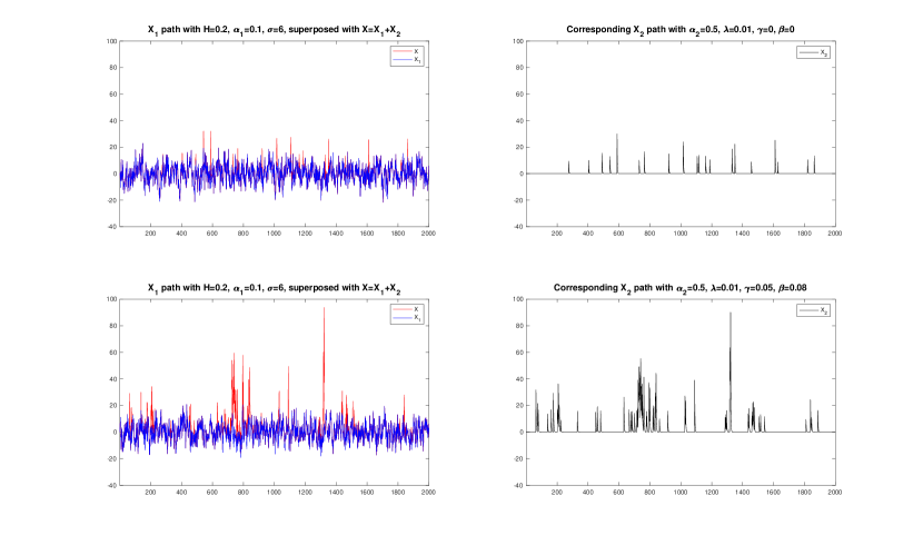
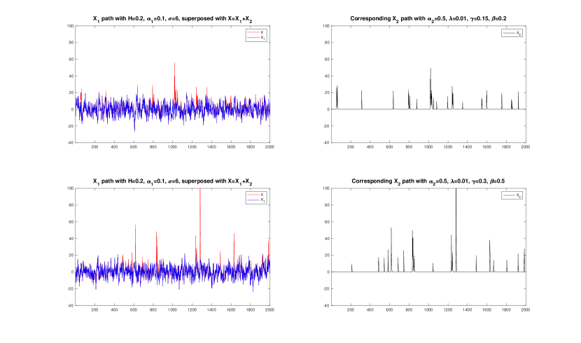
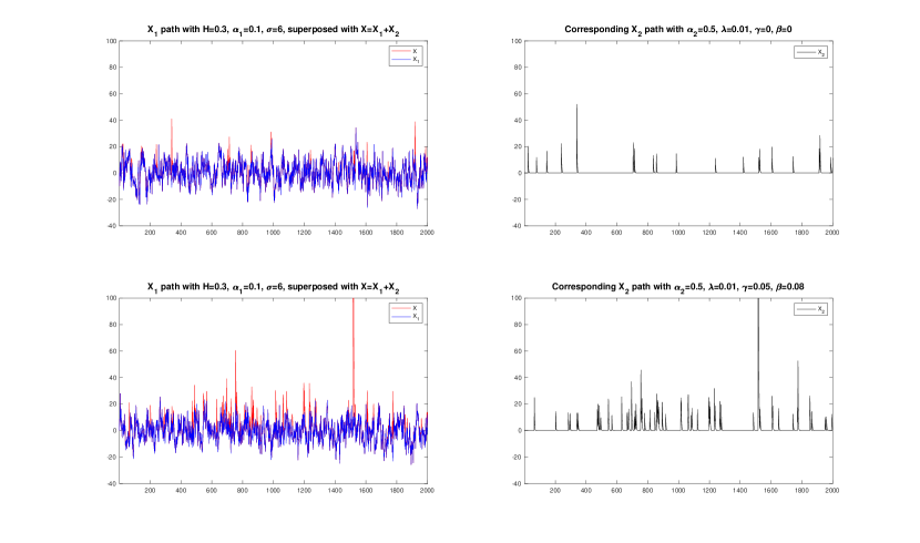
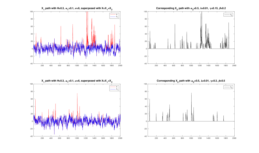
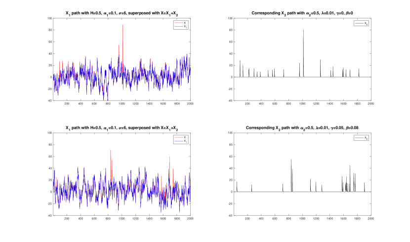
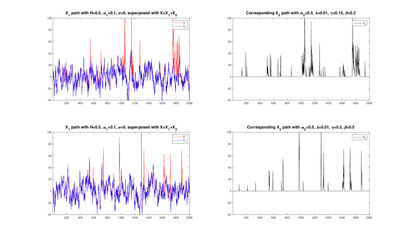
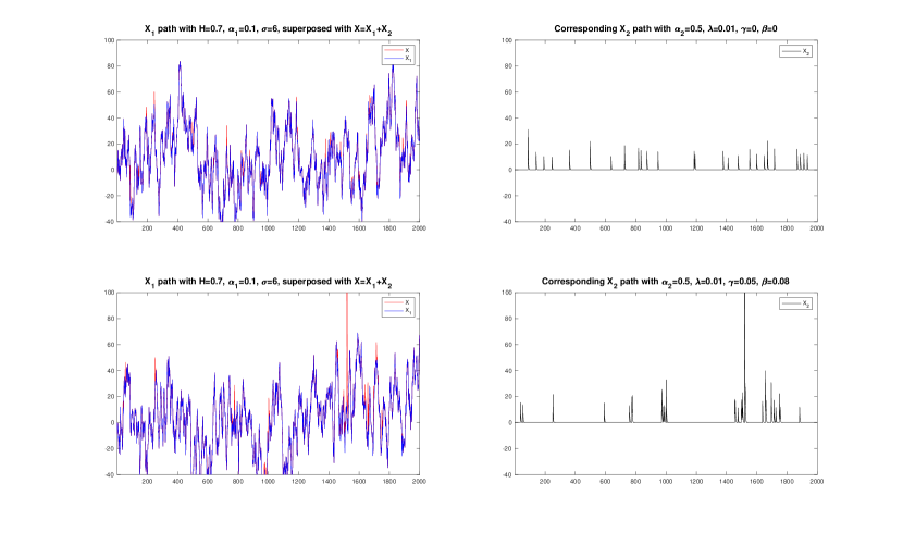
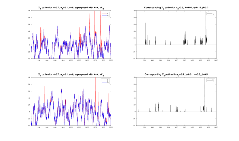
Even if in some cases this meant that some parts of the path are not visible, we chose to keep the same scale in all figures. This makes us see very clearly the differences caused in the nature of the process $X_{1}$ by the changes in the values of $H$. We see in particular that, keeping $\alpha_{1},\sigma$ fixed we get a much more variable process as long as $H$ increases.

Regarding the jump component $X_{2}$, which is independent from $X_{1}$, we see that the cluster effect is clearly visible for the sets of parameters (b)–(d). It seems that the set of parameters (b) is producing more clusters than the others. This may seem strange, since in this case the parameter $\gamma$ is lower than in (c) and (d), but we remark that in all cases the parameter $\beta$, which models the speed of mean reversion of $\lambda_{t}$ towards $\lambda$, varies consistently with $\gamma$.

We make a remark about the relation of this simulations with the real data. If we compare Figures 1–8 with Figure 9, in which we plot the entire dataset that we will analyse, we can make some qualitative considerations. Our simulations of $X_{1}+X_{2}$ do not include any seasonal component, and this is clearly visible. Anyway, from the point of view of the appearance of the paths, we see some similarities between Figure 9, the bottom plot of Figure 3 and the top plot of Figure 4, which are relative to $H=0.3$ and the set of parameters (b) and (c) for the Hawkes process, corresponding to $\gamma=0.05,\,\beta=0.08$ and $\gamma=0.15,\,\beta=0.2$. In both of these figures the standard volatility seems quite similar to the one of the real data, and moreover the jump behaviour (both amplitude and clusters) is quite similar to the one of Figure 9.

These considerations are coherent with the estimates that we will get in Section 4.3.2.

3 Parameter estimation

This section is devoted to the methods of estimation for the parameters of the two stochastic components $X_{1}$ and $X_{2}$ of our model. We recall that we have the following set of parameters to be estimated from the dataset $Y$

Equation	Parameter
$\mathbf{X_{1}}$	$\alpha_{1}$
$\mathbf{X_{1}}$	$\sigma$
$\mathbf{X_{1}}$	$H$
$\mathbf{X_{2}}$	$\alpha_{2}$
$\mathbf{X_{2}}$	$\lambda_{0}$
$\mathbf{X_{2}}$	$\gamma$
$\mathbf{X_{2}}$	$\beta$
$\mathbf{X_{2}}$	parameters for jump distribution

Table 4: Parameters of the model

3.1 Estimations for $X_{1}$

For the base component $X_{1}$, we have to estimate three parameters: $\alpha_{1}$, which is the rate of mean-reversion of the process to the zero level, $\sigma$, which is the variance parameter of the fractional noise $B^{H}$, and the parameter of fractionality of the noise $H$ itself, which determines whether the contributions of the noise term are positively correlated (if $H>1/2$), negatively correlated (if $H<1/2$) or non-correlated (if $H=1/2$, which is the case in which the noise is a classical Brownian motion).

We discuss first the estimation of the Hurst exponent $H$. Its estimation is very important since it determines the magnitude of the self-correlation of the noise of our model. There are various techniques that can be used to infer the Hurst coefficient from a discrete signal. In [29] the reader may find a good reviewon the argument. Anyway, these techniques can be used to estimate the Hurst coefficient only by assuming that the observed path belongs only to a fractional Brownian motion $\{B_{t}^{H}(\omega)\}_{t}$, without any drift. So it is not our case. We use the estimator provided in [25], given the observations of a wide class of SDEs driven by fractional Brownian motion, including the case of an Ornstein-Uhlenbeck model.

Given the time interval of observation $[0,T]$, let us consider a partition $\pi_{n}=\left\{T\displaystyle\frac{k}{n}\right\}_{k}$, where ${k\in\{0,1,\ldots,n\}}$. Given a stochastic process $\{X_{1}\}_{t\in[0,T]}$, let us define the two step increment as follows

$$\Delta^{(2)}_{n,k}X_{1}:=X_{1}\left(\frac{k+1}{n}T\right)-2X_{1}\left(\frac{k}{n}T\right)+X_{1}\left(\frac{k-1}{n}T\right).$$

By Theorem 3.4 of [25], we have that the statistics

$$\hat{H}_{n}:=\frac{1}{2}-\frac{1}{2\log 2}\log\Bigg{(}\frac{\sum_{k=1}^{2n-1}(\Delta^{(2)}_{2n,k}X_{1})^{2}}{\sum_{k=1}^{n-1}(\Delta^{(2)}_{n,k}X_{1})^{2}}\Bigg{)}$$

is a strongly consistent estimator of $H$, i.e. it holds

$$\lim\limits_{T\to\infty}\hat{H}_{n}=H,a.s.$$

In our case, our dataset will be discretized in time steps with minimum length equal to one, so we will have to stop at a specific step of the discretization, which is exactly the maximum value of $n$ such that $\frac{T}{2n}>1$.

The estimation of the diffusion cpefficient $\sigma$ is based on the use of the $p$-the variation. Indeed for any $k\geq 2$ and for any $p\geq 1$, the estimator is defined as

$$\hat{\sigma}_{T}(n):=\frac{n^{-1+pH}V^{n}_{k,p}X_{1}(T)}{c_{k,p}T},$$ (28)

where $V_{k,p}^{n}X_{1}(t)$ is the $k$-th order $p$-th variation process defined by

$$V_{k,p}^{n}X_{1}(t) := \sum_{i=1}^{[nt]-k+1}\Big{|}\Delta_{k}X_{1}\Big{(}\frac{i-1}{n}\Big{)}\Big{|}^{p}$$

$$:= \sum_{i=1}^{[nt]-k+1}\Bigg{|}\sum_{j=0}^{k}(-1)^{k-j}\binom{k}{j}X_{1}\Big{(}\frac{i+j-1}{n}\Big{)}\Bigg{|}^{p}.$$

The constant $c_{k,p}$ in (28) is given by

$$c_{k,p}:=\frac{2^{p/2}\Gamma\Big{(}\frac{p+1}{2}\Big{)}}{\Gamma\Big{(}\frac{1}{2}\Big{)}}\rho_{k,H}^{p/2},$$

where $\rho_{k,H}$ is

$$\rho_{k,H}:=\sum_{j=-k}^{k}(-1)^{1-j}\binom{2k}{k-j}|j|^{2H}.$$

The estimator (28) has been introduced in [22]. With a discrete dataset of time lenght $N$ and with minimum discretization length equal to $1$, we can only compute the estimator $\hat{\sigma}_{T}(n)$ for $n=1$ and $T=N$. We choose to use $k=2$ and $p=2$.

Finally, the mean reverting parameter $\alpha_{1}$ has been estimated with the following ergodic estimator

$$\hat{\alpha}_{1}(T):=\Big{(}\frac{1}{\sigma^{2}H\Gamma(2H)T}\int_{0}^{T}X_{1}(t)^{2}dt\Big{)}^{-\frac{1}{2H}}.$$ (29)

It holds that [22]

$$\lim\limits_{T\to\infty}\hat{\alpha}_{1}(T)=\alpha_{1},\quad a.s.$$

The estimator (29) is continuous version, but it can be easily discretized. Suppose that we are observing our process $X_{1}$ in the time points $\{kh\}$, for $h=0,\dots,n$. Here $h$ is the amplitude of the time discretization, and we suppose that $h=h(n)$ is such that $hn\to\infty$ and $h(n)\to 0$ when $n\to\infty$. In [22] the authors define the discretized estimator as

$$\hat{\alpha}_{1}(n):=\Big{(}\frac{1}{\sigma^{2}H\Gamma(2H)T}\sum_{k=1}^{n}X_{1}(kh)^{2}\Big{)}^{-\frac{1}{2H}}.$$ (30)

The only difference with the continuous version is the discretization of the integral appearing in (29). The following result holds:

Theorem 3 ([22], Theorem 5.6).

Let $X_{1}$ be the solution of an Ornstein-Uhlenbeck process observed at times $\{kh,k=0,\dots,n\}$, and such that $h=h(n)$ satisfies $hn\to\infty$ and $h(n)\to 0$ when $n\to\infty$. Moreover, if we suppose that

• if $H\in(0,\frac{3}{4})$, $nh^{p}\to 0$ as $n\to\infty$ for some $p\in\Big{(}1,\frac{3+2H}{1+2H}\wedge(1+2H)\Big{)}$

• if $H=\frac{3}{4}$, $\frac{h^{p}n}{\log(hn)}\to 0$ as $n\to\infty$ for some $p\in(1,\frac{9}{5})$

• if $H\in(\frac{3}{4},1)$, $h^{p}n\to 0$ as $n\to\infty$ for some $p\in\Big{(}1,\frac{3-H}{2-H}\Big{)}$

Then the estimator $\hat{\alpha}_{1}\xrightarrow{n\to\infty}\alpha_{1}$ a.s.

We observe that in our case we are not able to extend the total length of the observation interval, since only a single time series is given. In addition, our dataset consists in daily observations, so that the minimum time increment $h$ that we can consider is $h=1$. We aim to define a proper function $h=h(n)$ such that it satisfies the conditions of Theorem 3 for every value of $H\in(0,1)$ (which is in principle unknown).

Let $N$ be the length of our dataset. As a fundamental condition, we want that $h(N)=1$, so that we are able to compute the $N$-th approximation of our estimator with our data. We look for our candidate $h$ within the class of functions

$$h(n)=\Big{(}\frac{N}{n}\Big{)}^{\delta},$$

for some positive $\delta$ to be determined. All $h$ in this class satisfy that $h(N)=1$. We need also need to have that $nh\to\infty$, as $n\to\infty$, which imposes the condition $\delta<1$. Moreover, we have to impose on $h$ conditions i), ii), iii) of Theorem 3. We compute

$$nh(n)^{p}=\frac{N^{p\delta}}{n^{p\delta-1}}.$$

In condition i) and iii) we need $nh^{p}\to 0$ as $n\to\infty$, while in ii) we need $\frac{nh^{p}}{\log(nh)}\to 0$. Since $\log(nh)\to\infty$ by hypothesis, the condition $nh^{p}\to 0$ is more restrictive and we impose it also in ii). Since we do not need a priori which is the value of $H$ of our fractional Ornstein-Uhlenbeck process $X_{1}$, we find a $p=p(H)$ that is a good choice for any value of $H\in(0,1)$. One can easily verify that $p(H)=1+H$ lies in all the admissible intervals for $p$ in i), ii), iii). With this choice of $p$, the expression of $nh^{p}$ reads

$$nh(n)^{p}=\frac{N^{(1+H)\delta}}{n^{\delta(1+H)-1}}.$$

In order for the right-hand side to converge to zero we must have $\delta>\frac{1}{(1+H)}$. So we are left with the pair of conditions

$$\frac{1}{1+H}<\delta<1,$$

which are both satisfied if we define

$$\delta=\delta(H):=\frac{1}{(1+H)^{\frac{1}{2}}},$$

for any $H\in(0,1)$. With this choice of $h$, we are able to calculate the $N$-th step of the approximation of $\alpha_{1}$, regardless of the estimation $\hat{H}$ of $H$ that we obtained. Furthermore, in the definition of $\hat{\alpha}_{1}(n)$ there is a clear dependence on $\sigma$, which in our case is unknown. We remark that anyway, since the estimator $\hat{\sigma}$ converges a.s. to $\sigma$ as the order of the approximation increases, we have that the estimator $\hat{\alpha}_{1}$ converges a.s. to $\alpha_{1}$ also if we substitute $\hat{\sigma}$ to $\sigma$ in its definition.

Case	$\hat{\alpha}_{1}$	$q_{5\%}(\hat{\alpha}_{1})$	$q_{95\%}(\hat{\alpha}_{1})$
a.1	0.1069	0.0050	0.2523
a.2	0.1030	0.0220	0.2098
a.3	0.1017	0.0445	0.1737
a.4	0.1019	0.0531	0.1641
Case	$\hat{\sigma}$	$q_{5\%}(\hat{\sigma})$	$q_{95\%}(\hat{\sigma})$
a.1	6.2334	5.7834	6.7926
a.2	6.2313	5.7705	6.8007
a.3	6.2233	5.7024	6.8636
a.4	6.1976	5.4920	7.0783
Case	$\hat{H}$	$q_{5\%}(\hat{H})$	$q_{95\%}(\hat{H})$
a.1	0.1940	0.0885	0.2969
a.2	0.2927	0.1902	0.3931
a.3	0.4909	0.3982	0.5819
a.4	0.6882	0.6024	0.7715

Table 5: Estimated parameters of the component $X_{1}$, given $M=20000$ realizations of the component $X_{1}$ itself for each of the parameters set a.1 – a.4.

3.2 Estimations for $X_{2}$

For the jump component $X_{2}$, there are three separated tasks to carry out in order to estimate the parameters of the model. First, one has to estimate the parameters of the self-exciting intensity of the Hawkes process. Second, one has to choose and fit an adequate distribution for the jump magnitude. Third, one has to estimate the mean-reverting parameter $\alpha_{2}$ appearing in (26).

We start with the parameters of the jump intensity $\lambda_{t}$ defined in (17). In [33] the author gives an explicit formula for the log-likelihood of $\lambda,\gamma,\beta$, the parameters of the intensity function $\lambda_{t}$, given the observed jump times $T_{i}$. The log-likelihood takes the form

$$L(T_{1},\dots T_{n}|\lambda,\gamma,\beta) = -\lambda T_{n}+\sum_{j=1}^{n}\frac{\gamma}{\beta}\left(e^{-\beta(T_{n}-T_{j})}-1\right)$$

$$+\sum_{j=1}^{n}\log\Big{(}\lambda+\gamma A(j)\Big{)},$$

where $A(1)=0,A(j)=\sum_{i=1}^{j-1}e^{-\beta(T_{j}-T_{i})},j\geq 2$. In order to have a more efficient maximization process, one can immediately compute the partial derivatives of $L$. One has

$$\frac{\partial\log L}{\partial\gamma} = \sum_{j=1}^{n}\frac{1}{\beta}\left(e^{-\beta(T_{n}-T_{j})}-1\right)+\sum_{i=j}^{n}\left[\frac{A(i)}{\lambda+\gamma A(i)}\right];$$

$$\frac{\partial\log L}{\partial\beta} = -\gamma\sum_{j=1}^{n}\left[\frac{1}{\beta}(T_{n}-T_{j})e^{-\beta(T_{n}-T_{j})}+\frac{1}{\beta^{2}}e^{-\beta(T_{n}-T_{j})}\right]$$

$$-\sum_{j=1}^{n}\left[\frac{\gamma B(i)}{\lambda+\gamma A(i)}\right];$$

$$\frac{\partial\log L}{\partial\lambda} = -T_{n}+\sum_{j=1}^{n}\left[\frac{1}{\lambda+\gamma A(i)}\right];$$

with

$$\frac{\partial^{2}\log L}{\partial\gamma^{2}} = -\sum_{i=j}^{n}\left[\frac{A(i)}{\lambda+\gamma A(i)}\right]^{2};$$

$$\frac{\partial^{2}\log L}{\partial\beta^{2}} = \gamma\sum_{j=1}^{n}\left[\frac{1}{\beta}(T_{n}-T_{j})^{2}e^{-\beta(T_{n}-T_{j})}+\frac{2}{\beta^{2}}(T_{n}-T_{j})e^{-\beta(T_{n}-T_{j})}\right.$$

$$\hskip 28.45274pt\left.+\frac{2}{\beta^{3}}\left(e^{-\beta(T_{n}-T_{j})}-1\right)\right]$$

$$+\sum_{i=j}^{n}\left[\frac{\gamma C(i)}{\lambda+\gamma A(i)}-\left(\frac{\gamma B(i)}{\lambda+\gamma A(i)}\right)^{2}\right];$$

$$\frac{\partial^{2}\log L}{\partial\lambda^{2}} = -\sum_{j=1}^{n}\left[\frac{1}{\left(\lambda+\gamma A(i)\right)^{2}}\right];$$

$$\frac{\partial^{2}\log L}{\partial\beta\partial\gamma} = -\sum_{j=1}^{n}\left[\frac{1}{\beta}(T_{n}-T_{j})e^{-\beta(T_{n}-T_{j})}+\frac{1}{\beta^{2}}\left(e^{-\beta(T_{n}-T_{j})}-1\right)\right]$$

$$+\sum_{i=j}^{n}\left[\frac{\gamma A(i)B(i)}{\left(\lambda+\gamma A(i)\right)^{2}}-\frac{B(i)}{\lambda+\gamma A(i)}\right];$$

$$\frac{\partial^{2}\log L}{\partial\gamma\partial\lambda} = -\sum_{i=j}^{n}\left[\frac{A(i)}{\left(\lambda+\gamma A(i)\right)^{2}}\right];$$

$$\frac{\partial^{2}\log L}{\partial\beta\partial\gamma} = \sum_{i=j}^{n}\left[\frac{\gamma B(i)}{\left(\lambda+\gamma A(i)\right)^{2}}\right].$$

In the previous equation the functions $B$ and $C$ are defined as $B(1)=0,B(j)=\sum_{i=1}^{j-1}(T_{j}-T_{i})e^{-\beta(T_{j}-T_{i})},j\geq 2$ and $C(1)=0,C(j)=\sum_{i=1}^{j-1}(T_{j}-T_{i})^{2}e^{-\beta(T_{j}-T_{i})},$ $j\geq 2$. Since the log-likelihood is non-linear with respect to the parameters, the maximization if performed by using nonlinear optimazation tecniques [33].

Case	$\hat{\lambda}_{0}$	$q_{5\%}(\hat{\lambda}_{0})$	$q_{95\%}(\hat{\lambda}_{0})$
b.1 $\lambda_{0}=0.1$	0.0101	0.0061	0.0141
b.2 $\lambda_{0}=0.1$	0.0105	0.0059	0.0162
b.3 $\lambda_{0}=0.1$	0.0095	0.0057	0.0139
b.4 $\lambda_{0}=0.1$	0.0088	0.0053	0.0126
Case	$\hat{\gamma}$	$q_{5\%}(\hat{\gamma})$	$q_{95\%}(\hat{\gamma})$
b.1 $\gamma=0$	0.0046	3.84$\cdot 10^{-9}$	0.0267
b.2 $\gamma=0.05$	0.0366	0.0146	0.0606
b.3 $\gamma=0.15$	0.0840	0.0472	0.1217
b.4 $\gamma=0.3$	0.1163	0.0479	0.1850
Case	$\hat{\beta}$	$q_{5\%}(\hat{\beta})$	$q_{95\%}(\hat{\beta})$
b.1 $\beta=0$	0.6097	0.0407	0.8025
b.2 $\beta=0.08$	0.0814	0.0318	0.1379
b.3 $\beta=0.2$	0.1414	0.0846	0.2113
b.4 $\beta=0.5$	0.2782	0.1393	0.4421

Table 6: Estimated parameters of the component $X_{2}$, given $M=20000$ realizations of the component $X_{2}$ itself for each of the parameters set b.1 –b.4.

.

We see that the estimated values are below the true values, especially for big values of $\gamma,\beta$. For the set of parameters (a), the value of $\beta$ is largely overestimated, but this is not a problem since the corresponding value of $\gamma$ are very small, and thus there is no observable self-excitement.

Regarding the jump magnitude distribution, we fit the data via an MLE procedure by considering a Generalized Extreme Value (GEV) distribution. It is a continuous distribution which may seen as the approximation of the maxima of sequences of of independent and identically distributed random variables. It depends upon three parameters which allow to fit properly the data.

Finally, the estimation of the mean-reverting parameter $\alpha_{2}$ of the jump component $X_{2}$ can be done by using the estimator defined in [27]. Given a dataset $Y_{2}$ which we aim to model with our jump process $X_{2}$, a consistent estimator for the mean-reversion parameter $\alpha_{2}$ is

$$\hat{\alpha}_{2}=\log\Big{(}\max_{1\leq j\leq N}\frac{Y_{2}(j-1)}{Y_{2}(j)}\Big{)}.$$ (31)

We will need an approximation of this estimator in our estimation process, which is very closely related to one made in [27]. The details will be discussed during the data filtering process in the next section.

4 A study case: Italian electricity spot prices

Here we discuss the more strongly computational part of the work, by starting from the description of the time series we take into consideration, that is 8 year of daily recorded Italian electricity spot prices. We first perform an explorative analysis on the time series, and after that, we discuss the problem of data filtering that we need to solve in order to obtain from rough data the different components of our model. In the end, we perform out-of-sample simulationsin order to predict future prices of electricity, discussing the results with some evaluation metrics like Winkler score and Pinball loss function.

4.1 The time series

We consider the time series of the Italian Mercato del giorno prima (MGP, the day-ahead market), available at [40]. Figure 9 shows a plot of the daily price time series $\{Y(t)\}_{t=1,\ldots,3287}$ from January, $1^{\mathrm{st}}$ 2009 ($t=1$) to December, $31^{\mathrm{st}}$ 2017 ($t=3287$).

The MGP market is a day-ahead market, i.e. a market in which the price is established via an auction for the blocks of electricity to be delivered the following day. The agents that operate as buyers in the market have to submit their offers between 8:00 a.m. and 12:00 noon of the previous day. The offers regard the hourly blocks of electricity which will be delivered the following day. This means that an agent will submit 24 different offers (with different prices and quantities) for the electricity of the following day, and he will do it all at the same time. Also the sellers submit their offers, by telling the quantity of energy that they are willing to sell and the price at which they want to sell it. The market price is then established before 12:55 p.m., and it is an hourly price, determined by finding the intersection of the demand and the offer curve relative to the specific hour of the day. After the determination of the market price, all the electricity bought and sold for that hour is traded at the market price.

Figure 9: The time series $Y(t)$ of the the daily electricity prices in the MGP in the period 2009, January 1- 2017, December 31 ($t=1,\ldots,3287$).

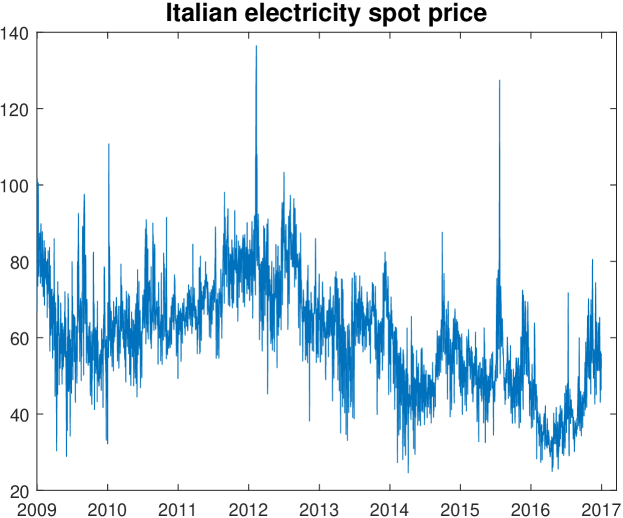
We choose to model the daily average of the hourly price. This is a quite common choice in the literature, especially for reduced-form models [39]. Indeed, the main scope of reduced–form models is to be able to capture more the medium term (days/weeks) distribution of prices than the hourly price, and to use these estimated distributions of prices to pricing electricity future contracts, which are very useful and used financial instruments in the electricity market.

We are aware that this averaging filters out many extreme behaviours of the market. Indeed, a single hourly extreme price is unlikely to produce a significant variation in the average daily price. Anyway, we are also aware that reduced–form models usually perform poorly on the hourly scale [39]. We remark that all the analysis that follows has been carried out also using on–peak (08:00–20:00) and off–peak (20:00–08:00) data separately, without obtaining a significant difference from the entire day averages.

The data available start from April, 2004, which is the moment in which the liberalised electricity market started in Italy, but we chose to focus on more recent data, from 2009 onwards, to make the model more tight to the present nature of the electricity market. This does not prevent the performance evaluation of the model from being sufficiently robust, since the dimension of the sample is $N=3287$.

Figure 10: The daily electricity prices in the MGP whitin the calibration window in the period 2009, January 1- 2010, December 31 ($t=1,\ldots,730$).

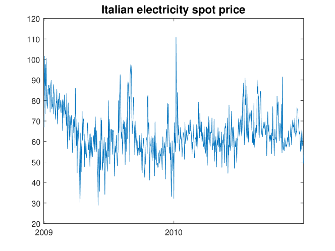
We use the data in the following way: the first $730$ days have been used for the study of the dataset and for the validation of the model. Then, we evaluated the performance on forecasting future prices for time horizons of length $h=1,\dots,30$, using rolling windows: at time $t$, we use the data from $t-730$ to $t$ for the calibration of the parameters of the model, and we simulate the future price at time $t+h$ using those parameters. Then, we move ahead from time $t$ to $t+h$ and we repeat the previous steps, starting from parameter estimation.

The first task that has to be achieved is the separation, or filtering, of the different signals in the price time series $Y$. It is clear that this is not an easy task and it might not be done in a unique way. In literature a lot of effort has been done for this purpose (see [23, 30, 39, 28, 27, 31]). Moreover, we think that in the present case the relatively small presence of clearly recognisable spikes in the dataset makes the spike identification task even more difficult than usual.

Note that from now on we consider as the window for the calibration of the model the one corresponding to the first two years, 2009 and 2010. The reduced time series $Y(t),t\in[1,730]$ is shown in Figure 10.

4.2 Data filtering

Weekly seasonal component. The first component that should be identified and estimated is the one dealing with trends and seasonality in the data. As stated in [23] and in the literature therein, the estimation routines are usually quite sensitive to extreme observations, i.e. the electricity price spikes. Hence, one should first filter out the spikes, that often are identified by the outliers. Actually, whether to filter out the spikes before or after the identification of the deterministic trends is still an open question in general. Furthermore, the deseasonalizing methods used in literature are very different: some authors suggest to considered sums of sinusoidal functions with different intensities [9, 16, 27], others consider piecewise constant functions (or dummies) for the month [15, 26], or the day [13] or remove the weekly periodicity by subtracting the average week [23]. It turns out than an interesting and more robust technique is the method of wavelet decomposition and smoothing, applied among others in [23, 30, 37, 38].

Figure 11: Autocorrelation function of the daily electricity price returns. (a) Full series 2009, January 1- 2017, December 31. (b) Prices within the calibration window 2009, January 1- 2010, December 31.

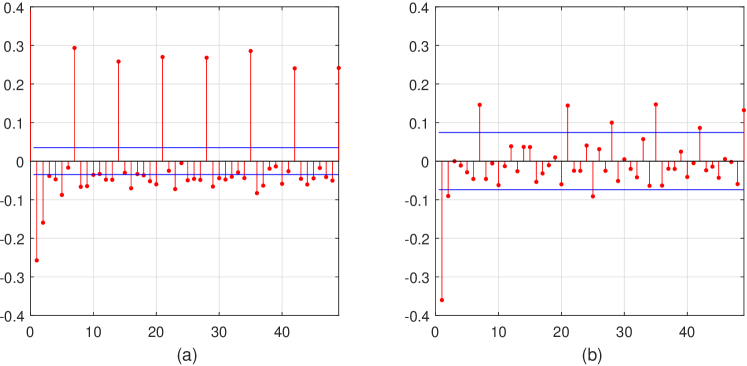
Figure 11 shows the autocorrelation function both for the whole series and within the calibration window. In the first case, for any lag multiple of seven the correlation is statistically significant, while in the calibration windows only for the lag=14 there is not a significant correlation at the level $95\%$. In any case the presence of weekly periodicity is clear. As a consequence we first filter the weekly periodicity. As in [13, 39] we do it by means of dummy variables, which take constant value for each different weekday. Hence, we subtract the average week calculated as the sample mean of the sub-samples of the prices corresponding to each day of the week, as in [23]. Public holidays are treated in this study as the eighth day of the week. Hence, the total number of dummies is eight.

More precisely, we define a function $D=D(t)$ which determines which label the $t$-th day has, i.e. $D(t)=i,i=1,,\ldots,7,8$, if day $t$ correspond to Monday (and not a festivity), …, Sunday (and not a festivity) and a festivity, respectively. We define the restricted time series $Y_{D=j}$ as the time series formed only by the price values labelled with the day $j$, and with $\overline{Y_{D=j}}$ its arithmetic mean. Then we define the whole dummy variables function $Y_{D}$ as

$$Y_{D}(t)=\sum_{j=1}^{8}1_{D(t)=j}(t)\overline{Y_{D=j}}.$$ (32)

Figure 12: (a) Original prices $Y$ (green) and prices after dummies removal $Y_{w}$ (blue); (b) Autocorrelation of the returns of the prices $Y_{w}$

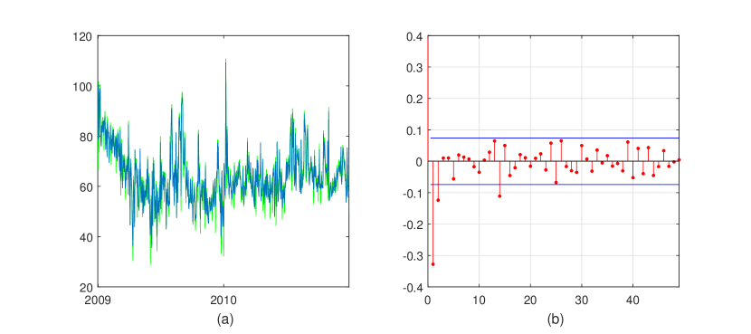
The time series obtained after the weeekly deseasonalization is the following

$$Y_{w}(t):=Y(t)-\hat{f}_{s}(t)=:Y(t)-(Y_{D}(t)-\overline{Y}),$$ (33)

where $\overline{Y}$ is the arithmetic mean of $Y(t),t=1,...,730.$ The arithmetic mean of the prices $Y_{w}$ corresponding to a specific day of the week coincides with the mean of all prices within the calibration window. Figure 12-(a) shows that $Y_{w}$ after removing the dummy variables is barely distinguishable from the original time series $Y$; it is only a bit more regular. On the other hand, $Y_{w}$ does not show weekly correlation, as visible in Figure 12-(b). The function $\hat{f}_{s}$ is the estimate of the short seasonality in $f$.

Jump component. Before filtering the long-term seasonal component, we filter out the jump component. The reason for this order lies in the following consideration: at a small scale, the presence of a slowly moving seasonal trend does not affect the recognition of a price spike. On the other hand, if we chose to filter the long-term seasonal component before filtering out the spikes, the presence of one of more spikes could affect the form of the seasonal component, which is something that we intuitively regard as incorrect. Indeed, we tend to consider the spikes as an ”external event”, and we do not want the seasonal term to be affected by the presence of a price spike.

As in [27], the idea is to obtain the filtered time series, denoted $Y_{J}$, as the series that contains the jumps and their paths of reversion towards their mean. We first estimate the mean-reversion speed $\alpha_{2}$ by the estimator $\hat{\alpha}_{2}$ given by (31); by performing the estimate along the entire time series, not only in the jump times: this is not restrictive, since the strongest rates of reversion towards the mean happen right after a jump has occurred. Afterwards we identify the jump times. The idea is to consider as jumps the price increments that exceed $k$ standard deviations of the price increments time series. This cannot be implemented to the time series $Y_{w}$ directly, because, in case two spikes appear one after the other, the second one would not be considered as a spike. In order to avoid this effect, we define the modified time series $\tilde{Y}_{w}$ as

$$\widetilde{Y}_{w}(t):=(1-\alpha_{2})Y_{w}(t)+\hat{\alpha}_{2}\bar{Y}_{30}(t),$$

where $\bar{Y}_{30}(t)$ is the moving average of the time series $Y_{w}$ over periods of 30 days. Then, we defined the times series

$$\left\{Y_{w}(t)-\widetilde{Y}_{w}(t-1)\right\}-{t=2,3,\ldots}$$ (34)

of the modified increments, which takes into account a reversion effect towards the moving average $Y_{30}$. It performs very well also when the spikes appear in clusters. Then, denoted by $\widetilde{\sigma}$ the standard deviation of the series (34), we say that a spike occurs at time $\tau$ if

$$\left|Y_{w}(\tau)-\widetilde{Y}_{w}(\tau-1)\right|>2.5\widetilde{\sigma}.$$ (35)

If $N$ is the number of detected spikes, i.s. if $\left\{\tau_{j}\right\}_{j=1,\ldots,N}$ are the times satisfying condition (35), the corresponding jumps are defined, for $j=1,\ldots,N$ as

$$\hat{\mu}_{j}=Y_{w}(\tau_{j})-\widetilde{Y}_{w}(\tau_{j}-1).$$

Once we have the estimates $\left\{(\tau_{j},\hat{\mu}_{j})\right\}_{j=1,\ldots,N}$ of the times and magnitudes (10) of the jumps, we obtain the estimation $Y_{J}(t)$ of the solution $X_{2}$ of (26) as follows

$$Y_{J}(t)=\sum_{j=1}^{N}\mu_{j}e^{-\hat{\alpha}_{2}(t-\tau_{j})}\epsilon_{\tau_{j}}([-\infty,t])$$ (36)

Given $Y_{J}$ as in (36), we denote the filtered time series as

$$Y_{s}(t)=Y_{w}(t)-Y_{J}(t).$$

Long-term seasonal component. Now we look for an estimator $\hat{f}_{l}$ of the long-term seasonality component, so that

$$\hat{f}=\hat{f}_{s}+\hat{f}_{l},$$

where $\hat{f}_{s}$ is given in (33), is an estimator of the deterministic part $f$ in (2). There is a lot of literature on the subject (see, for example, [7, 9, 13, 16, 23, 26, 38]). These references try to explain such a component by means of sinusoidal functions or sums of sinusoidal functions of different frequencies. In our case it seems that there is no statistically significant dependence upon such periodic function, both in the case of monthly, half-yearly or yearly periodicity.

We apply the method of wavelet decomposition and smoothing, applied among others in [23, 30, 37, 38]. The idea is to consider repeatedly the convolution of $Y_{s}$ with a family of wavelets, which have the effect of smoothing out $Y_{s}$. If we manage to smooth $Y_{s}$ enough to remove the effect of stochastic oscillation, but not too much to remove the long-term trend, then we can subtract this smoothed version of $Y_{s}$ from $Y_{s}$ itself, obtaining a centred time series with almost no long-term oscillation.

Figure 13: Price series $Y_{S}$ (blue) and estimation function $\hat{f}_{l}$ (red) via Daubechies of order 24 wavelets at level 8.

We go more into details: we refer to [30] and the literature therein. We use wavelets belonging to the Daubechies family, of order 24, denoted by (F–db24). Wavelets of different families and orders make different trade-offs between how compactly they are localized in time and their smoothness. Any function or signal (here, $Y_{s}$) can be built up as a sequence of projections onto one father ($W$) wavelet and a sequence of mother wavelets ($D$): $Y_{s}=W_{k}+D_{k}+D_{k-1}+...+D_{1}$, where $2^{k}$ is the maximum scale sustainable by the number of observations. At the coarsest scale the signal can be estimated by $W_{k}$. At a higher level of refinement the signal can be approximated by $W_{k-1}=W_{k}+D_{k}$. At each step, by adding a mother wavelet $D_{j}$ of a lower scale $j=k-1,k-2,...,$ one obtain a better estimate of the original signal. Here we use $k=8$, which corresponds a quasi-annual ($2^{8}=256$ days) smoothing. Then the estimator $\hat{f}_{l}$ of the long-term deterministic part $f-\hat{f}_{s}$ is given by

$$\hat{f}_{l}(t)=W_{8}(t),$$ (37)

the Daubechies wavelets of order 24 at level 8.

The resulting time series $Y_{f}$ given by

$$Y_{f}(t)=Y_{s}(t)-\hat{f}_{l}(t),$$ (38)

represents a realization of the base component $X_{1}$.

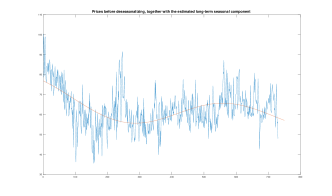
Figure 13 show the price series $Y_{s}$ and the overlapped estimated $\hat{f}_{l}$. The wavelet interpolation is here extended outside the calibration window. This is not automatic in the case of wavelet decomposition, since the wavelets are compactly supported and we are convolving only up to the final time of our dataset. To obtain this prolongation, we prolonged the time series in the forecasting window by using the technique of exponential reversion to the median, thoroughly studied in [30], before applying the wavelet de-noising. In this way we have been able to obtain a function $\hat{f}_{l}$ which extends also to times $t$ in the forecasting windows.

4.3 Out of sample simulations

We will perform and assess here the forecasts of future electricity prices through our model. We first outline the simulation scheme and make some considerations about the parameters in the rolling windows. After this, we define the metrics which we will subsequently use to evaluate our results.

4.3.1 Parameter estimation in the rolling windows

We recall that for each time $t$, when forecasting the price distribution at time $t+h$ (where $h\in\{1,\dots,30\}$ is the forecasting horizon), we carry out a new calibration of all the parameters of the model, including the Hurst coefficient $H$. We think that in this way, if there is a change in the data coming as input, the model is able to change its fine structure coherently with these changes. For example, if the self–correlations changes, or disappears, at some point, we expect the parameter $H$ to change consequently, and possibly approach $\frac{1}{2}$.

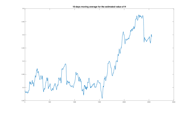
We start by analysing $H$: as long as our rolling window for estimation is advancing,the values of $H$ are on average increasing. The first estimate is $\hat{H}=0.2909$. The mean value across the whole dataset is $0.3735$. In general, the values are such that

$$0.2128\leq\hat{H}\leq 0.6234.$$

Notice that the maximum value is above the $H=1/2$ threshold and this shows that a positive correlation between the increments may occur. Figure 14 shows the pver ten days averaged behaviour of $H$ across all time lengths in.

In general, as we already pointed out, we think that this moving identification of the parameter $H$ is useful to update the fractional structure of the model when the input data are suggesting to do so, giving a better modelling flexibility, also in case of future changes in the market nature.

Figure 14: 10-day average of the estimated value $\hat{H}$ of $H$. We chose the 10-day average in order to smooth out some irregular behaviour at shorter scale.

Regarding the parameters of the fractional Ornstein–Uhlenbeck process $X_{1}$, $\alpha_{1}$ and $\sigma$, progressing in our rolling window, we found a change in the estimated values of the parameters; summarizing, we obtained that the range of values for $\hat{\alpha}_{1}$ and $\hat{\sigma}$

$$\begin{split}&0.0453\leq\hat{\alpha}_{1}\leq 0.6823\\ &4.2069\leq\hat{\sigma}\leq 8.8972.\end{split}$$

We see that there is a large variation in the parameters, especially for $\hat{\alpha}_{1}$, but we remark that this variation is gradual, since the mean reversion rate decreases while moving through our forecasting dataset, together with the volatility $\hat{\sigma}$. Looking at Figure 9, this can be observed, at least for the volatility, also by a macroscopic observation of the data.

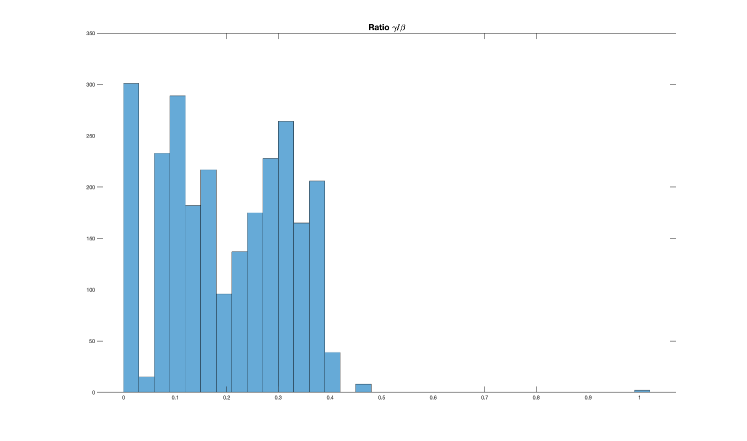
Looking at the estimation of the parameters of the jump process $X_{2}$, a bit of variability through the dataset is shown, but there is not an evidence of a particular pattern. Moreover, the jump observations are relatively rare (20-40), so based on the available data, it would be even more difficult to draw conclusions on their long term behaviour. The estimated values of the mean–reversion coefficient $\alpha_{2}$ are suche that $\hat{\alpha}_{2}\in[0.3564,0.6211]$, with an the mean value $0.4358$. As the Hawkes process parameter estimation regards, $\hat{\lambda}_{0}\in[0.0101,0.0284]$ with mean value $0.0169$, $\hat{\gamma}\in[1.12\cdot 10^{-9},0.1574]$, with mean their mean $0.0625$ and $\hat{\beta}\in[0.0012,0.9993]$ with mean $0.3662$. There is a great variation in such estimates. This, in our opinion, is due to the low dimension of the dataset, because not many spikes are present. Thus, the MLE method is finding sometimes a good evidence of a self-excitement (when $\gamma$ is bigger and relatively close to $\beta$) and sometimes no evidence of self-excitement (when $\gamma$ is very small and/or $\beta$ is much bigger than $\gamma$). To show this fact, we plot in Figure 15 an histogram of the ration $\gamma/\beta$, which is a very good indicator of the presence of self-excitement. From the histogram, we can see that roughly half of the time the ratio is below 0.25 (showing little or no self-excitement), and half of the time above (showing a significant self-excitement). We think this is another evidence of the flexibility of our model, similarly to the estimations of $H$. If some self-excitement seems to be present, then the model is including it. Otherwise, the model will simply produce a classical point process with constant intensity.

Figure 15: Ratio between $\hat{\gamma}$ and $\hat{\beta}$ throughout the entire dataset.

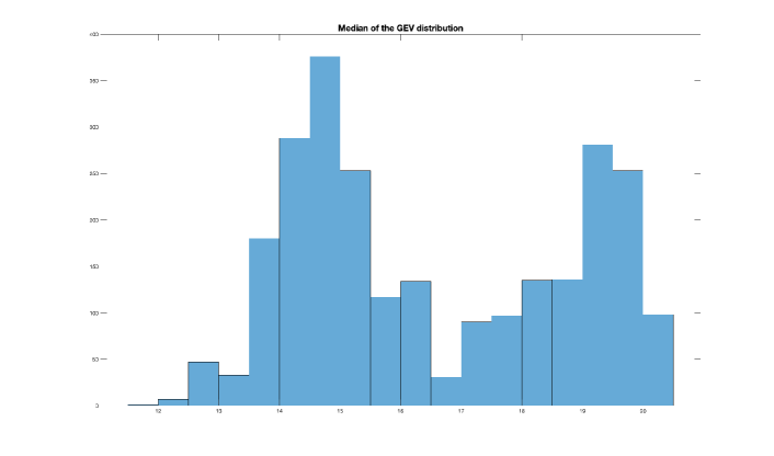
As the estimation of the parameters $(\tilde{\mu},\xi,\tilde{\sigma})$ of the Generalized Extreme Value distribution we have that $\hat{\tilde{\mu}}\in[11.2506,19.4064]$ with a mean value $15.6687$, $\hat{\xi}\in[-0.4809,4.2591]$ with mean $0.4125$ and $\hat{\tilde{\sigma}}\in[0.3248,3.8260]$ with mean $2.2331$. We only remark that even if there is a great variability in the parameters, the median value of the jump size is not varying from one estimate to the other. We recall that the median (the mean is not always defined) of a GEV distribution is given by

$$\text{Median}=\mu+\sigma\frac{\log(2)^{-\xi}-1}{\xi}.$$

In Figure 16, we see that this value is oscillating between 11 and 22, which are reasonable values for our dataset.

Figure 16: Median of the GEV distribution throughout the entire dataset.

4.3.2 Forecasting performance

Now we evaluate the performance of the model described in Section 2 for the forecast of future values of the electricity prices. As pointed out in [39], there is no universal standard procedures for evaluating the forecasts.

The most widely used technique is to obtain point forecasts, i.e. single forecast values, and evaluate them using some error function. The most common error function for this type of forecasts is Mean Absolute Percentage Error (MAPE), together with its refinement Mean Absolute Scaled Error (MASE). Another frequently used measure is the Root Mean Square Variation (RMSV), which is simply the estimated standard variation of the forecast error. In our model, the SDE-type structure is not particularly suitable for giving short-term point forecasts, as it is also pointed out in [39]. So in the following we will not concentrate our analysis on point forecasts, as we do not expect our model to be able to outperform more sophisticated and parameter-rich model in this task.

We focus on the relatively novel concept of Interval Forecast. More recently, as was already suggested in [39] and as it has been more thoroughly analized in the very recent review [31], the driving interest in forecast evaluation has been put in interval forecasts and density forecasts. Interval forecast have also been used as the official evaluating system in 2014’s Global Energy Forecasting Competition (GEFCom2014). There is a close relation between interval forecasts and density forecasts.

Interval forecasts (also called Prediction intervals, shortly PI) are a method for evaluating forecasts which consists in constructing the intervals in which the actual price is going to lie with estimated probability $\alpha$, for $\alpha\in(0,1)$. There are many technique for the construction of the intervals and their evaluation [31]. Here we consider interval forecasts for different time lags $h$, by means of different techniques: Unconditional Coverage (UC), Pinball loss function (PLF) and Winkler Score (WS).

Unconditional Coverage (UC). Establishing the UC just means that we evaluate nominal rate of coverage of the Prediction intervals; as stated in [31], one can simply evaluate this quantity, or consider the average deviation from the expected rate $\alpha$. As pointed out in [31], if we call $P_{t}$ the actual price, $[\hat{L_{t}},\hat{U_{t}}]$ the Prediction interval at level $\alpha\in(0,1)$, we are checking the fact that the random variable

$$I_{t}=\begin{cases}1,&\text{if }P_{t}\in[\hat{L_{t}},\hat{U_{t}}],\\ 0,&\text{if }P_{t}\notin[\hat{L_{t}},\hat{U_{t}}],\\ \end{cases}$$

has a Bernoulli $B(1,\alpha)$ distribution. This works clearly under the assumption that the violations are independent, which may not always be the case.

Pinball loss function (PLF). The Pinball loss function is a scoring function which can be calculated for every quantile $q$. If we denote with $P_{t}$ the actual price, with $Q_{q}(\hat{P_{t}})$ the $q$-th quantile of the estimated prices $\hat{P_{t}}$ obtained with the model, the Pinball loss function is defined as

$$\begin{split}\text{Pin}(Q_{q}(\hat{P_{t}}),P_{t},q):=\begin{cases}(1-q)(Q_{q}(\hat{P_{t}})-P_{t}),&\text{if }P_{t}<Q_{q}(\hat{P_{t}}),\\ q(P_{t}-Q_{q}(\hat{P_{t}})),&\text{if }P_{t}\geq Q_{q}(\hat{P_{t}}).\end{cases}\end{split}$$

Winkler Score (WS). The Winkler score is a scoring rule similar to the Pinball loss function, with the aim of rewarding both reliability (the property of having the right share of actual data inside the $\alpha$-th interval) and sharpness (having smaller intervals). For a central $\alpha$-th interval $[\hat{L_{t}},\hat{U_{t}}]$, $\delta_{t}:=\hat{U_{t}}-\hat{L_{t}}$, and for a true price $P_{t}$, the WS is defined as

$$\text{WS}([\hat{L_{t}},\hat{U_{t}}],P_{t})=\begin{cases}\delta_{t},&\text{if }P_{t}\in[\hat{L_{t}},\hat{U_{t}}],\\ \delta_{t}+\frac{2}{\alpha}(P_{t}-\hat{U_{t}}),&\text{if }P_{t}>\hat{U_{t}},\\ \delta_{t}+\frac{2}{\alpha}(\hat{L_{t}}-P_{t}),&\text{if }P_{t}<\hat{L_{t}}.\\ \end{cases}$$

As it can be seen, the WS has a fixed part which depends only on the dimension of the Prediction intervals.

Comparison of different models. We checked the performance not only of the model proposed in Section 2, but of two more models, in order to highlight the peculiarities of the model proposed in this paper. The examined models are the following.

• The stochastic differential equations described in Section 2 in which the base component is driven by a fractional Brownian motion.

• The same model as in i) in which instead of the fractional Brownian motion, the standard Brownian motion is considered.

• A naive model, built as Naive(t)=D(t)+H, where $D$ is the dummy variables function and $H$ is randomly sampled historical noise coming from the relative calibration window [31].

Forecasting horizons. As already mentioned, used as the calibration window a rolling window with fixed dimension of $730$ prices, corresponding to the $730$ days of past observations. In this framework, we will consider the following forecasting horizons $h$:

$$h=\{1,2,\dots,29,30\}$$

For each forecasting horizon we make a new estimate of the parameters at a distance $h$ from the previous one, in order to have the sampled prices coming from disjoint time intervals.

4.3.3 Results

We start by analysing the performance of the models by their observed Unconditional Coverage. Figure 17 shows their performance in a plot which spans across all the forecasting horizons $h$ that we are considering. The dotted black line represents the relative level of coverage that we should attain. The closer we are to the dotted line, the more accurate a model is in covering that specific interval.

In the $50\%$ interval (top plot), the naïve model seems to be more stable, even if it is almost always under-covering the interval. Among our models, the fBm model, except for the shorter forecasting horizons, is performing remarkably well. The sBm model is over-covering the interval, for almost all forecasting horizons.

Figure 17: Observed Unconditional Coverage of the model with the fractional Brownian motion (blue), with the standard Brownian motion (red) and the naive one (yellow)) for $50\%,90\%$ and $98\%$ coverage intervals. On the horizontal axis, we represent the length $h$ of the forecasting window we are considering, while on the vertical axis we represent the UC value.

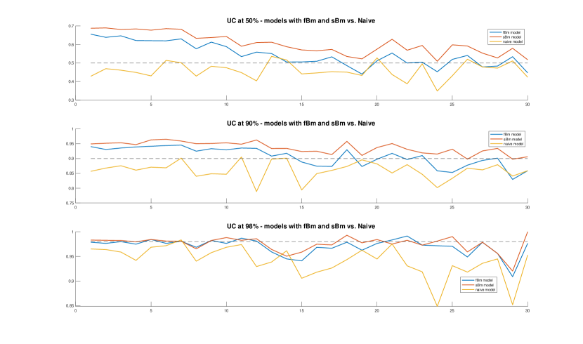
Moving to the $90\%$ (mid plot) and $98\%$ (bottom plot) prediction intervals, the fBm model performs in general better than the other ones, except for a slight excess in coverage for the $90\%$ PI with small forecasting windows. In the $98\%$ prediction intervals, also the sBm model has a very good performance, which will be confirmed by the numerical data for the Unconditional Coverage reported in Table 7.

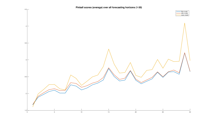
We analysed then the Pinball loss function and Winkler Score of the three models. In Figure 18 and in Figure 19 we reported again the results spanning along all forecasting horizons. We note that the Pinball loss function is a function of the quantile we are evaluating, so that in principle we would have to evaluate it separately for every quantile $q=1,\dots,99$. As it has also been done in the GEFCom2014 competition, we averaged first over all quantiles, in order to obtain a single value and make comparisons easier.

In terms of the Winkler scores (Figure 18), the fBm and the sBm models outperform the the naïve benchmark. The difference between the fBm model and the sBm model is very small in general, but the fBm model performs better than the sBm one in almost every prediction interval. This is true especially if we consider the $90\%$ interval WS.

Figure 18: Winkler scores for $50\%$ and $90\%$ PI. Again, on the horizontal axis, we represent the length $h$ of the forecasting window we are considering, while on the vertical axis we represent the Winkler score value.

Figure 19: Pinball loss function (average).On the horizontal axis, we represent the length $h$ of the forecasting window we are considering, while on the vertical axis we represent the Pinball loss function value.

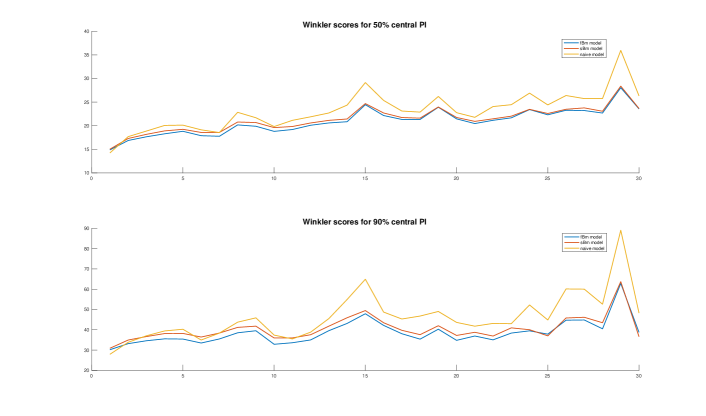
There seems to be a sort of contradiction in our results: indeed, when it comes to the UC at level $50\%$, the naïve model seemed to be slightly better than the fBm model, while in terms of WS for the $50\%$ PI the fBm is clearly superior to the naïve benchmark. This is possible because the WS is a metric which not only evaluates the share of coverage of a prediction interval, but also gives a penalty for missed values, and this penalty depends on the magnitude of the error made. Thus, it is seem reasonable to suppose that the naïve model, while performing quite good in terms of coverage at the $50\%$ PI, makes bigger errors than the fBm model.

The results about the Pinball loss function are quite similar to the ones of the Winkler scores. Again, the fBm and the sBm model outperform the naïve model, while being very close one to each other. Again, the fBm model performs slightly better than the sBm model.

Both in terms of WS and Pinball loss function, the naïve model is performing better than the fBm and the sBm model when the forecasting horizon $h=1$. This is somewhat consistent with a fact mentioned in [39], which we already reported: the reduced-form models, like ours, usually have a quite poor performance in very short-term forecasts.

Avg. score\Model	fBm	sBm	Naïve
$UC_{50\%}$	$54.54\%$	$60.37\%$	$\mathbf{46.02\%}$
$UC_{50\%}$ error	$+4.54\%$	$+10.37\%$	$\mathbf{-3.98\%}$
$UC_{50\%}$ abs. error	$5.95\%$	$10.37\%$	$\mathbf{4.83\%}$
$UC_{90\%}$	$\mathbf{90.63\%}$	$93.65\%$	$86.02\%$
$UC_{90\%}$ error	$\mathbf{-0.93\%}$	$-9.10\%$	$+3.79\%$
$UC_{90\%}$ abs. error	$\mathbf{2.81\%}$	$3.67\%$	$4.04\%$
$UC_{98\%}$	$97.02\%$	$\mathbf{97.58\%}$	$94.13\%$
$UC_{98\%}$ error	$-0.98\%$	$\mathbf{-0.42\%}$	$3.87\%$
$UC_{98\%}$ abs. error	$1.19\%$	$\mathbf{0.99\%}$	$3.90\%$

Table 7: Coverage rate for the estimated PI, averaged over all forecasting horizons $h=1,\dots,30$. The average error, as it can be seen, is just the difference of the average coverage from the nominal value.

Score \Model	fBm	sBm	Naïve
WS50%	$\mathbf{20.87}$	$21.30$	$23.14$
WS90%	$\mathbf{38.62}$	$40.44$	$46.25$
PLF	$\mathbf{2.3484}$	$2.3920$	$2.6164$

Table 8: Winkler scores and Pinball loss function values, averaged over all forecasting horizons $h=1,\dots,30$.

In Table 7 and Table 8 we reported the above discussed values, averaged over all different forecasting horizons. In terms of the UC, each of the three models is performing better than the others for a certain PI, while both for the WS and the PLF we see the better performance of the fBm model also from these numerical data.

4.4 Conclusions

Drawing some conclusions from the results analyzed above, there are some evidences that a fBm-driven model may be more adequate to model the electricity prices than a sBm-driven model.

Regarding the forecasting performance (QF and PI), the fBm methods have better performance than the sBm ones in terms of WS and PLF, while both the sBm and the naïve model enjoy some success when evaluating the UC.

To understand this apparent contradiction, we remark (as we already did) that WS and PLF are scoring rules which give a penalty for missed forecasts (while UC does not), and these penalties depend also on the magnitude of the error. The fact that fBm models outperform sBm models in this evaluation may mean that the QF and the PI given by the fBm models are in some sense more robust than the sBm ones (and also than the ones of the naive benchmark).

Concerning the model structure, we remark that we found very satisfactory the fact that the parameter estimation for the Hawkes process gave roughly half of the times a very significant value, meaning that the clustering effect is not only visible on a macroscopic scale, but is also captured by the numerical methods.

This was not assured in principle, since the Italian market is rather peculiar, having only a small number of real spikes. This gives, as a consequence, that the intensity of the spike process is small and could become difficult to estimate, even if this was not the case for our data.

Regarding the role of the fractional Broenian motion in the model, we remark that we found some very interesting informations from the estimation procedure. The fact, shown in Figure 14, that the parameter $H$ is tending to $0.5$ in more recent times may mean that the market is finding automatically a way towards the ”independence of increments”, which would be implied by the fact that $H=0.5$. This is remarkable also for the fact that the independence of increments is closely related, for these models, with the absence of arbitrage. Even if we pointed out that arbitrage is usually not possible, for this kind of models, when trading only once per day, a good question for future developments in this sense may be: are electricity markets, which are ”young” financial markets, finding their own stability with the passing of time, or are our findings specific to the italian market? In any case, are these changes going to last in the future or we may see a return of a fractional effect in the next years?

References

- [1] Bacry, E. and Muzyd, J.F., Hawkes model for price and trades high-frequency dynamics, Quant. Financ. 14, 1147–1166, (2014).
- [2] Bacry, E., Mastromatteo, I., and Muzyd, J.F., Hawkes processes in Finance, Market Microstructure and Liquidity, 1, (2015).
- [3] Barndorff-Nielsen, O.E., Benth, F.E. and Veraart, A. Modelling energy spot prices by volatility modulated Levy driven Volterra processes, Bernoulli, 19, 803–845, (2013).
- [4] Becker R., Clements, A. E. and Zainud, W.N., Modeling electricity price events as point processes, J. Energy Markets, 6, (2013).
- [5] Benth, F.E., Benth, J.S., Koekebakker, S., Stochastic modelling of electricity and related markets, World Scientific Publishing, (2008).
- [6] Benth, F. E., Kallsen J. and Meyer-Brandis T., A Non-Gaussian Ornstein-Uhlenbeck Process for Electricity Spot Price Modeling and Derivatives Pricing, Appl. Math. Finance, 14, 153–169, (2007).
- [7] Benth, F.E., Kiesel, R. and Nazarova A., A critical empirical study of three electricity price models, EnĖconom. 34, 1589–1616, (2012).
- [8] Brémaud P. and Massoulié, L., Stability of nonlinear Hawkes processes, Ann. Probab. 24, 1563–1588, (1996).
- [9] Cartea, A. and Figueroa, M. Pricing in electricity markets: a mean reverting jump diffusion model with seasonality, Appl. Math. Financ. 12, 313–335, (2005).
- [10] Chen, J., Hawkes, A.G., Scalas, E., and Trinh, M. Performance of information criteria for selection of Hawkes process models of financial data, Quant. Fin. 18, 225–235, (2018).
- [11] Cheridito, P. Arbitrage in fractional Brownian motion models. Fin. Stoc. 7, 533–-553, (2003).
- [12] Da Fonseca, J. and Zaatour, R., Hawkes Process: Fast Calibration, Application to Trade Clustering, and Diffusive Limit, J. FutṀark. 34, (2014).
- [13] De Jong, C., The nature of power spikes: a regime-switch approach, Stud. Nonlinear Dyn. E. 10, (2006).
- [14] Delattre, S., Fournier,N., and Hoffman M., Hawkes Processes on Large Networks, Ann. Appl. Probab. 26, 216–261, (2016).
- [15] Fleten, S.–E., Heggedal, A.M. and Siddiqui, A., Transmission capacity between Norway and Germany: a real options analysis, J. Energy Markets, 4, 121–147, (2011).
- [16] Geman, H. and Roncoroni, A., Understanding the fine structure of electricity prices, J. Bus. 79, 1225–1261, (2006).
- [17] Gianfreda, A. and Grossi, L.,Fractional integration models for Italian electricity zonal prices, Advances in Theoretical and Applied Statistics. Studies in Theoretical and Applied Statistics. Springer, Berlin, Heidelberg, 429–440, (2013).
- [18] Hainaut D., Clustered Lévy processes and their financial applications. J. Comp. Appl. Math. 319, 117-1-40, (2017).
- [19] Hawkes. A.G., Point spectra of some mutually exciting point processes, J. Royal StatṠoc. 33, 438–443, (1971).
- [20] Hawkes. A.G., Spectra of some self-exciting and mutually exciting point processes, Biometrika, 90, 58–83, (1971).
- [21] Hawkes, A.G., Hawkes processes and their applications to finance: a review. Quantitative Finance, 18, 2, 2018
- [22] Hu, Y., Nualart, D. and Zhou, H., Parameter estimation for fractional Ornstein-Uhlenbeck processes of general Hurst parameter, Stat. Inference Stoch. Process., 22, 1–32, (2017).
- [23] Janczura, J., Trück, S., Weron, R. and Wolff, R.C., Identifying spikes and seasonal components in electricity spot price data: A guide to robust modelling, En. Econ. 38, 96–110, (2013).
- [24] Jao, Y., Ma, C., Scotti, S. and Sgarra, C., A branching process approach to power markets, En. Mark. 79, 144–156, (2018).
- [25] Kubilius, K., Mishura, Y. and Ralchenko, K., Parameter Estimation in Fractional Diffusion Models, Bocconi & Springer series 8, (2017).
- [26] Lucia, J.J. and Schwartz, E.S., Electricity prices and power derivatives: evidence from the nordic power exchange, Rev. Derivat. Resear. 5, 5–50, (2002).
- [27] Kluppelberg, C., Meyer-Brandis, T. and Schmidt, A., Electricity spot price modelling with a view towards extreme spike risk, Quantit. Fin. 10, 963–974, (2010).
- [28] Meyer-Brandis T. and Tankov, P., Multi-factor jump-diffusion models of electricity prices, Int. J. Theor. Appl. Finan. 11, (2008).
- [29] Mielniczuk, J.,, Wojdyłło, P., Estimation of Hurst exponent revisited, Comput. Stat. & Data Anal. 51, 4510–4525, (2007)
- [30] Nowotarski,J., Tomczyk, J. and Weron, R., Estimation and forecasting of the long–term seasonal component of electricity spot prices, En. Econom. 39, 13–27, (2013).
- [31] Nowotarski, J. and Weron, R., Recent advances in electricity price forecasting: A review of probabilistic forecasting, Renew. Sustain. En. Rev. 81, 1548–1568, (2018).
- [32] Ogata, Y. On Lewis’ Simulation Method for Point Processes, Trans. Inform. Th. 27, (1981).
- [33] Ozaki, T. Maximum Likelihood estimation of Hawkes’ self-exciting point process, Ann. Inst. Statist. Math. 31, 145–155, (1979).
- [34] Rogers, L.C.G.. Arbitrage with fractional Brownian motion, Math. Fin. 7, 95–105, (1997).
- [35] Roncoroni, A., Fusai, G. and Cummins, M., Handbook of Multi-Commodity Markets and Products, Wiley, (2015).
- [36] Schwartz, E.S., The stochastic behavior of commodity prices: implications for valuation and hedging, J. Finance, 52, 923–973, (1997).
- [37] Weron, R., Modeling and Forecasting Electricity Loads and Prices: a Statistical Approach, Wiley, (2006).
- [38] Weron, R., Market price of risk implied by Asian-style electricity options and futures, Energy Econ. 30, 1098–1115, (2008).
- [39] Weron, R., Electricity price forecasting: A review of the state-of-the-art with a look into the future, Internat. J. Forecas. 30, 1030–1081, (2014).
-
[40]
The Italian MPG data.
http://www.mercatoelettrico.org/It/download/DatiStorici.aspx