Modified HLLC-VOF solver for incompressible two-phase fluid flows

Abstract

A modified HLLC-type contact preserving Riemann solver for incompressible two-phase flows using the artificial compressibility formulation is presented. Here, the density is omitted from the pressure evolution equation. Also, while calculating the eigenvalues and eigenvectors, the variations of the volume fraction is taken into account. Hence, the equations for the intermediate states and the intermediate wave speed are different from the previous HLLC-VOF formulation [Bhat S P and Mandal J C, J. Comput. Phys. 379 (2019), pp. 173-191]. Additionally, an interface compression algorithm is used in tandem to ensure sharp interfaces. The modified Riemann solver is found to be robust compared to the previous HLLC-VOF solver, and the results produced are superior compared to non-contact preserving solver. Several test problems in two- and three-dimensions are solved to evaluate the efficacy of the solver on structured and unstructured meshes.

Sourabh P. Bhat	J. C. Mandal
spbhat.mail@gmail.com https://spbhat.in/	mandal@aero.iitb.ac.in https://www.aero.iitb.ac.in/~mandal/

1 Introduction

The artificial compressibility formulation is a commonly accepted way of solving single-phase incompressible fluid flows [1, 2, 3, 4, 5, 6, 7, 8]. However, the artificial compressibility formulation is less common in solving multiphase incompressible flows [9, 10, 11, 12]. In the original paper on artificial compressibility formulation by Chorin [13], the mass equation is converted into a pressure evolution equation by adding an artificial term. This ingenious technique allowed for the pressure to evolve with the velocity field in a closely-coupled manner. The said paper and the others following this formulation use a non-dimensional form of governing equations and hence do not include density in the mass equation. However, when applying this technique for solving two-phase flows there is no unique density to normalize, and hence there are two possibilities. One is to use the conservative variable in mass equation as $p/\left(\rho\beta\right)$ [12, 14] and the other method is to omit the density and use $p/\beta$ [9, 15, 16, 17], where $p$ is the pressure, $\rho$ is the fluid density and $\beta$ is the artificial compressibility parameter. In our recent paper [14], we presented a contact preserving HLLC-type Riemann solver, for incompressible two-phase flows using $p/\left(\rho\beta\right)$ in the mass equation, which was called HLLC-VOF solver. In this follow-up paper, a contact preserving Riemann solver for the second type of system using $p/\beta$ is presented. This modification seems to result in a more robust solver. Because, in contrast to HLLC-VOF solver, the modified solver works well with a single chosen value of $\beta$, in all the considered test problems. Also, in the modified Riemann solver, the density in the momentum variables is written as a function of volume fraction when evaluating the eigenvalues and eigenvectors of the flux Jacobian. Hence, the convective flux obtained by the modified Riemann solver is considerably different compared to the previous HLLC-VOF solver.

Calculation of the convective flux using a Riemann solver (instead of a geometric method such as the PLIC [18]) has many advantages, as Riemann solvers are independent of cell geometry. The formulation remains same irrespective of the cell type, geometry complexity and the number of physical dimensions. However, due to the upwind nature of Riemann solvers, some numerical dissipation inherently gets added to the flux, which helps in stabilizing the numerical scheme. The HLLC-type contact-preserving Riemann solvers are less dissipative and do not smear the fluid interface much, for small duration of evolution. Therefore, in the earlier paper [14] this issue was not addressed. However, this is not acceptable in problems evolving for a long duration, or where the fluid interfaces move very slowly. This is a well-known shortcoming and few techniques are available in literature to mitigate this problem, such as the FCT method [19] and the CICSAM method [20]. Another approach for reducing the numerical dissipation is to superimpose a compressive velocity field over the existing velocity field, such that the interface thickness gets restricted. This is done by adding an artificial compressive term to the VOF equation [21, 22], which is active only near the interface. This method is used in OpenFOAM software [23] and further advances are made to this method to ensure correct compressive flux [24, 25]. In this paper, the interface compression methodology is adopted as it fits naturally within the underlying framework.

To evaluate the efficacy of the modified solver, which we refer to as HLLC-VOF-M, various problems are solved on structured and unstructured mesh. The problems are chosen systematically such that only a few aspects of the solver are tested at a time. The solutions produced by the HLLC-VOF-M solver are compared with a non-contact capturing solver, experimental, theoretical and numerical solutions depending on availability of results in the literature. A three-dimensional problem involving merging of complex interfaces is also solved to demonstrate the extensibility of the present solver.

The remaining paper is organized as follows. We begin by describing the governing equations for two-phase incompressible fluid flows in the next section. The numerical formulation is given in section 3, and it comprises of nine sub-sections: finite volume method, treatment of time derivatives, convective flux, interface compression, viscous flux, surface tension, source term, initial conditions, and boundary conditions. Out of these nine sub-sections, our main contribution is in sub-section 3.3.2, where a detailed description of the HLLC-VOF-M Riemann solver is presented for calculation of the convective flux. Section 4 provides a brief overview and a flowchart of the complete algorithm used by the solver. Five numerical test problems, of varying nature, are presented and discussed in section 5. Finally, we conclude in section 6, by summarizing the key contributions from the paper.

2 Governing equations

The governing equations for 3-dimensional, unsteady incompressible two-phase flows, using dual-time stepping, artificial compressibility formulation and volume of fluid method, can be written as,

$$\begin{array}[]{c}{\displaystyle\frac{\partial\mathbf{U}}{\partial\tau}+\frac{\partial\mathbf{W}}{\partial t}+\frac{\partial\mathbf{F}}{\partial x}+\frac{\partial\mathbf{G}}{\partial y}+\frac{\partial\mathbf{H}}{\partial z}+\nabla\cdot\mathbf{F}_{c}=\frac{\partial\mathbf{F_{v}}}{\partial x}+\frac{\partial\mathbf{G_{v}}}{\partial y}+\frac{\partial\mathbf{H_{v}}}{\partial z}+\nabla\cdot\mathbf{T}+\mathbf{S}};\\ \mathbf{U}=\left[\begin{array}[]{c}p/\beta\\ \rho u\\ \rho v\\ \rho w\\ C\end{array}\right],\ \mathbf{W}=\left[\begin{array}[]{c}0\\ \rho u\\ \rho v\\ \rho w\\ C\end{array}\right],\ \mathbf{F}=\left[\begin{array}[]{c}u\\ \rho u^{2}+p\\ \rho uv\\ \rho uw\\ uC\end{array}\right],\ \mathbf{G}=\left[\begin{array}[]{c}v\\ \rho uv\\ \rho v^{2}+p\\ \rho vw\\ vC\end{array}\right],\ \mathbf{H}=\left[\begin{array}[]{c}w\\ \rho uw\\ \rho vw\\ \rho w^{2}+p\\ wC\end{array}\right],\\ \mathbf{F_{v}}=\left[\begin{array}[]{c}0\\ 2\mu\frac{\partial u}{\partial x}\\ \mu\left(\frac{\partial u}{\partial y}+\frac{\partial v}{\partial x}\right)\\ \mu\left(\frac{\partial u}{\partial z}+\frac{\partial w}{\partial x}\right)\\ 0\end{array}\right],\ \mathbf{G_{v}}=\left[\begin{array}[]{c}0\\ \mu\left(\frac{\partial u}{\partial y}+\frac{\partial v}{\partial x}\right)\\ 2\mu\frac{\partial v}{\partial y}\\ \mu\left(\frac{\partial v}{\partial z}+\frac{\partial w}{\partial y}\right)\\ 0\end{array}\right],\ \mathbf{H_{v}}=\left[\begin{array}[]{c}0\\ \mu\left(\frac{\partial u}{\partial z}+\frac{\partial w}{\partial x}\right)\\ \mu\left(\frac{\partial v}{\partial z}+\frac{\partial w}{\partial y}\right)\\ 2\mu\frac{\partial w}{\partial z}\\ 0\end{array}\right],\ \mathbf{S}=\left[\begin{array}[]{c}0\\ \rho g_{x}\\ \rho g_{y}\\ \rho g_{z}\\ 0\end{array}\right];\end{array}$$ (1)

where, $\tau$ is a pseudo-time variable used for iterating to a converged solution at a particular real-time $t$. $\mathbf{U}$ is the conservative variable vector updated in pseudo-time, $\mathbf{W}$ is the conservative variable vector updated in real-time, $\left(\mathbf{F},\mathbf{G},\mathbf{H}\right)$ are convective flux vectors, $\nabla\cdot\mathbf{F}_{c}$ is the interface compression term, $\left(\mathbf{F_{v}},\mathbf{G_{v}},\mathbf{H_{v}}\right)$ are the viscous flux vectors, $\mathbf{S}$ is a vector containing source terms and $\mathbf{T}$ is a tensor for surface tension force. The variable $p$ denotes pressure, $\beta$ is the artificial compressibility parameter, $\left(u,v,w\right)$ is the velocity vector in $\left(x,y,z\right)$ Cartesian space co-ordinates, $\rho$ is the density of the fluid, $\mu$ is the dynamic viscosity of the fluid and $\left(g_{x},g_{y},g_{z}\right)$ is the acceleration due to gravity. It may be noted that the conservative variable $p/\beta$ in the mass equation is an artificial term added for coupling the mass and momentum equations. Also, this modification converts the pseudo-time derivative along with the convective flux into a hyperbolic system. Hence, Riemann solvers can be used for calculation of convective flux.

The numerical simulation of two-phase flow, brings in an additional fifth equation for advection of volume fraction, $C$, and a tensor associated with surface tension $\mathbf{T}$. The details of surface tension are explained in sub-section 3.6. An interface compression term, $\nabla\cdot\mathbf{F}_{c}$ is introduced to ensure sharp interfaces, the details of which are given in sub-section 3.4. The density, $\rho$, and the dynamic viscosity, $\mu$, are defined as a function of volume fraction as,

$$\rho=\rho\left(C\right)=\rho_{1}\,C+\rho_{2}\,\left(1-C\right)=\left(\rho_{1}-\rho_{2}\right)\,C+\rho_{2},$$ (2)

$$\mu=\mu\left(C\right)=\mu_{1}\,C+\mu_{2}\,\left(1-C\right)=\left(\mu_{1}-\mu_{2}\right)\,C+\mu_{2}$$ (3)

where, $\rho_{1}$ is the density of first fluid, $\rho_{2}$ is the density of the second fluid, $\mu_{1}$ is the dynamic viscosity of the first fluid and $\mu_{2}$ is the dynamic viscosity of the second fluid.

3 Numerical formulation

3.1 Finite volume method

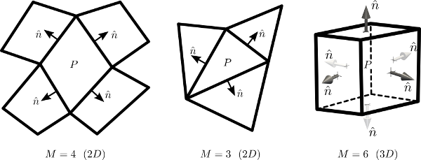
The finite volume discretization of the governing equations (1) is obtained by integrating the equations over an arbitrary volume in space. The volume of a cell $P$ is denoted as $\Omega_{P}$. Different types of cells used in this work are shown in Fig. 1. Using the Gauss-divergence theorem, the volume integrals reduce to surface integrals resulting in the following discretized form of the governing equations.

$$\Omega_{P}\,\frac{\partial\overline{\mathbf{U}}}{\partial\tau}+\Omega_{P}\,\frac{\partial\overline{\mathbf{W}}}{\partial t}+\sum_{m=1}^{M}\left(\mathbf{F}\,n_{x}+\mathbf{G}\,n_{y}+\mathbf{H}\,n_{z}\right)_{m}\,\Gamma_{m}+\sum_{m=1}^{M}\left(\mathbf{F}_{c}\cdot\hat{n}\,\Gamma\right)_{m}\\ =\sum_{m=1}^{M}\left(\mathbf{F_{v}}\,n_{x}+\mathbf{G_{v}}\,n_{y}+\mathbf{H_{v}}\,n_{z}\right)_{m}\,\Gamma_{m}+\sum_{m=1}^{M}\left(\mathbf{T}\cdot\hat{n}\,\Gamma\right)_{m}+\Omega_{P}\,\overline{\mathbf{S}}\ .$$ (4)

The over-bar indicates cell averaged value of a variable inside cell $P$. The cell is enclosed by $M$ planar faces, denoted by $m=1\dots M$, with the $m^{\text{th}}$ face having a surface area of $\Gamma_{m}$. The unit normal vector $\hat{n}=\left(n_{x},n_{y},n_{z}\right)$ for each of the planar faces points outward of the cell $P$. It may be noted that, in case of a second order accurate finite volume method, the cell-averaged values can be obtained by evaluating the variables at cell-centroid [26].

Fig. 1: Schematic diagrams for displaying the notations used in finite volume formulation.

3.2 Treatment of pseudo and real time derivatives

The dual-time stepping procedure proposed by Jameson [27] for compressible flows can be utilized along with the artificial compressibility formulation to obtain a time accurate solution for incompressible flows. The basic pseudo-compressibility procedure followed here is similar to the one described by Gaitonde [4]. The finite volume formulation (4) can be re-written as an ordinary differential equation (ODE) in pseudo-time as,

$$\Omega_{P}\frac{d\overline{\mathbf{U}}}{d\tau}=-R\left(\overline{\mathbf{U}}\right)\ ,$$ (5)

where, $R\left(\overline{\mathbf{U}}\right)$ is called the residual of cell $P$ and can be written as,

$$R\left(\overline{\mathbf{U}}\right)=\Omega_{P}\,\frac{\partial\overline{\mathbf{W}}}{\partial t}+\sum_{m=1}^{M}\left(\mathbf{F}\,n_{x}+\mathbf{G}\,n_{y}+\mathbf{H}\,n_{z}\right)_{m}\,\Gamma_{m}+\sum_{m=1}^{M}\left(\mathbf{F}_{c}\cdot\hat{n}\,\Gamma\right)_{m}\\ -\sum_{m=1}^{M}\left(\mathbf{F_{v}}\,n_{x}+\mathbf{G_{v}}\,n_{y}+\mathbf{H_{v}}\,n_{z}\right)_{m}\,\Gamma_{m}-\sum_{m=1}^{M}\left(\mathbf{T}\cdot\hat{n}\,\Gamma\right)_{m}-\Omega_{P}\,\overline{\mathbf{S}}\ .$$ (6)

Based on the ODE given by equation (5), the solution is updated in pseudo-time using the two-stage stability preserving Runge-Kutta method [28], which can be written as,

$$\begin{array}[]{rcl}\mathbf{U}^{\left(0\right)}&=&\mathbf{\overline{U}}^{k};\\ \mathbf{U}^{\left(1\right)}&=&\mathbf{U}^{\left(0\right)}-\frac{\Delta\tau}{\Omega_{P}}\,R\left(\mathbf{U}^{\left(0\right)}\right);\\ \mathbf{U}^{\left(2\right)}&=&\frac{1}{2}\,\mathbf{U}^{\left(0\right)}+\frac{1}{2}\,\mathbf{U}^{\left(1\right)}-\frac{1}{2}\,\frac{\Delta\tau}{\Omega_{P}}\,R\left(\mathbf{U}^{\left(1\right)}\right);\\ \mathbf{\overline{U}}^{k+1}&=&\mathbf{U}^{\left(2\right)};\end{array}$$ (7)

where, $\mathbf{U}^{\left(1\right)}$, $\mathbf{U}^{\left(2\right)}$ are the solutions at intermediate pseudo-time steps, $\mathbf{\overline{U}}^{k}$ is the solution at current pseudo-time and $\mathbf{\overline{U}}^{k+1}$ is the updated solution in pseudo-time. The pseudo-time iterations are carried out until the $L_{2}$-norm of the residual is reduced to a very small value, of $10^{-3}$, for all the conservative variables. Thus recovering the original unsteady two-phase flow equations, such that $\partial\overline{\mathbf{U}}/\partial\tau\approx 0$. The $L_{2}$-norm of the residual is defined as given by Wang et. al [29]. It may be noted that all the above variable vectors are functions of $\overline{\mathbf{U}}$, i.e. $\overline{\mathbf{W}},\mathbf{F},\mathbf{G},\mathbf{H},\mathbf{F}_{c},\mathbf{F_{v}},\mathbf{G_{v}},\mathbf{H_{v}},\mathbf{T}$ and $\overline{\mathbf{S}}$ are dependent on $\overline{\mathbf{U}}$. Hence, updating $\overline{\mathbf{U}}$ will modify the residual at every Runge-Kutta step.

The real-time derivative is numerically approximated using a three-point implicit backward difference formula, which can be easily derived to be,

$$\frac{\partial\overline{\mathbf{W}}}{\partial t}=\frac{3\,\overline{\mathbf{W}}^{k}-4\,\overline{\mathbf{W}}^{n}+\overline{\mathbf{W}}^{n-1}}{2\Delta t}\ .$$ (8)

where, $\Delta t$ is the chosen time step to evolve the solution in real-time (this time step is problem dependent and is defined for each problem in section 5, namely Results and discussion), $k$ denotes the current solution in pseudo-time, $n$ denotes the current solution in real-time, $n-1$ denotes the previous solution in real-time. The solution at previous real-time level is not available at the beginning of the simulation, hence, a two-point backward difference approximation is used. The two-point backward difference approximation can be written as,

$$\frac{\partial\overline{\mathbf{W}}}{\partial t}=\frac{\overline{\mathbf{W}}^{k}-\overline{\mathbf{W}}^{n}}{\Delta t}\ .$$ (9)

The pseudo-time step size, $\Delta\tau$, is limited by the stability requirements of the scheme. The pseudo-time step is dependent on the convective flux, viscous flux and the surface tension flux. Therefore,

$$\Delta\tau\leq\min\left(\Delta\tau_{cv},\Delta\tau_{s}\right)$$ (10)

where, $\Delta\tau_{cv}$ is the time step constraint due to convective and viscous flux, and $\Delta\tau_{s}$ is the time step constraint imposed by surface tension. The largest time step for a cell $P$ due to convective and viscous fluxes may be estimated using [30, 31, 32]

$$\left(\Delta\tau_{cv}\right)_{P}=\frac{\Omega_{P}}{\left(\Lambda_{c}+K\Lambda_{v}\right)_{P}}\ ,$$ (11)

where, $\Lambda_{c}$ and $\Lambda_{v}$ are estimates of the convective and viscous spectral radii for the cell respectively. The spectral radii are calculated as,

$$\Lambda_{c}=\sum_{m=1}^{M}\left(\max\left|\lambda\right|\,\Gamma\right)_{m}\quad\text{ and }\quad\Lambda_{v}=\frac{4}{3\,\Omega_{P}}\sum_{m=1}^{M}\left(\frac{\mu}{\rho}\Gamma^{2}\right)_{m}\ ,$$ (12)

where, $\max\left|\lambda\right|$ is the maximum absolute eigenvalue at the face $m$, $K=4$ is an empirically determined coefficient in [30]. The time constraint due to surface tension is estimated based on the expressions given in [33, 34] to be,

$$\Delta\tau_{s}=\left[\frac{\left(\rho_{1}+\rho_{2}\right)\Omega_{P}}{\pi\,\sigma}\right]^{1/2}\ .$$ (13)

The pseudo-time step is further limited by the real-time step, $\Delta t$, which is estimated using linear stability analysis in [35] as,

$$\Delta\tau\leq\frac{2}{3}\Delta t\ .$$ (14)

Finally a scaling factor, similar to Courant number, is used to obtain the following expression for pseudo-time step,

$$\Delta\tau=\mbox{CFL}\left[\min\left(\Delta\tau_{cv},\Delta\tau_{s},\frac{2}{3}\Delta t\right)\right]\ .$$ (15)

The scaling factor of $\text{CFL}=1$ is used in all the simulations in this paper. A local-time stepping algorithm is used to accelerate the convergence, where the value of $\Delta\tau$ may be different for each cell based on the local flow field.

3.3 Calculation of convective flux

The novelty of this paper lies in the development of an HLLC-type Riemann solver, for calculation of convective flux for three-dimensional, incompressible two-phase flows, governed by equations (1). The finite volume formulation provides a discrete, cell-averaged conservative variable vector, $\overline{\mathbf{U}}$, for each cell. Using these discrete solution vectors, the calculation of the convective flux is done in two steps.

1. Solution reconstruction, where the discrete solution vectors in the neighborhood of the cell, are used to obtain a smooth distribution of solution vector inside each cell. This will potentially result in discontinuities in solution vectors at the cell faces, leading to Riemann problems at cell faces.

2. Solving the Riemann problem to compute the convective flux, using the newly developed HLLC-VOF-M Riemann solver, at the cell faces.

These two steps are explained in the next two sub-sections.

3.3.1 Solution reconstruction

The conservative variables are reconstructed, using the local cell averaged data, to obtain a smooth distribution inside each cell. This is done by using a truncated Taylor series approximation and a distance weighted least-square approach. Consider a subset of a computational grid, as shown in Fig. 2.

Fig. 2: Subset of computational grids consisting of mixed cell-types. The centroid of the cell in which the solution is being reconstructed is represented using $\bullet$ symbol and centroid of neighboring cells is represented using $\blacksquare$ symbol.

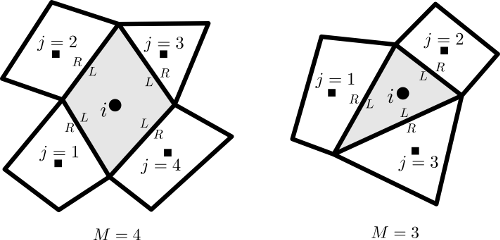
The cell, in which the solution reconstruction is carried out, is denoted as $i$ and the face-based neighboring cells are denoted as $j=1,2\dots M$. Let a scalar $\xi$ represent a single component from vector $\mathbf{U}$. A truncated Taylor series, about the centroid of cell $i$, can be written for approximating $\xi$ at the centroid of cell $j$ as,

$$\xi_{j}=\xi_{i}+\left.\frac{\partial\xi}{\partial x}\right|_{i}\Delta x_{j}+\left.\frac{\partial\xi}{\partial y}\right|_{i}\Delta y_{j}+\left.\frac{\partial\xi}{\partial z}\right|_{i}\Delta z_{j}$$ (16)

or the change in $\xi$ can be written as,

$$\Delta\xi_{j}=\left.\frac{\partial\xi}{\partial x}\right|_{i}\Delta x_{j}+\left.\frac{\partial\xi}{\partial y}\right|_{i}\Delta y_{j}+\left.\frac{\partial\xi}{\partial z}\right|_{i}\Delta z_{j}$$ (17)

where, $\Delta\xi_{j}=\left(\xi_{j}-\xi_{i}\right)$, $\Delta x_{j}=\left(x_{j}-x_{i}\right)$, $\Delta y_{j}=\left(y_{j}-y_{i}\right)$, $\Delta z_{j}=\left(z_{j}-z_{i}\right)$. The derivatives of $\xi$ are evaluated at the centroid of cell $i$. The second and higher order terms of the Taylor series are neglected, which results in a linear approximation. Writing the equations for $j=1\dots M$, produces $M$ linear equations and may be written as a over-determined system of equations,

$$\underbrace{\left[\begin{array}[]{ccc}\Delta x_{1}&\Delta y_{1}&\Delta z_{1}\\ \Delta x_{2}&\Delta y_{2}&\Delta z_{2}\\ \vdots&\vdots&\vdots\\ \Delta x_{M}&\Delta y_{M}&\Delta z_{M}\end{array}\right]}_{S}\underbrace{\left[\begin{array}[]{c}\left(\partial\xi/\partial x\right)_{i}\\ \left(\partial\xi/\partial y\right)_{i}\\ \left(\partial\xi/\partial z\right)_{i}\end{array}\right]}_{\nabla\xi_{i}}=\underbrace{\left[\begin{array}[]{c}\Delta\xi_{1}\\ \Delta\xi_{2}\\ \vdots\\ \Delta\xi_{M}\end{array}\right]}_{\Delta\xi}\ .$$ (18)

An inverse-distance based weights, $w_{j}=1/\left\|\Delta r_{j}\right\|_{2}$, are used to increase the influence of the nearby neighbors, where $\left\|\Delta r_{j}\right\|_{2}$ is the Euclidean distance between the points $i$ and $j$, calculated as,

$$\left\|\Delta r_{j}\right\|_{2}=\sqrt{\Delta x_{j}^{2}+\Delta y_{j}^{2}+\Delta z_{j}^{2}}\ .$$ (19)

The resulting weighted matrix may be written as,

$$W\,S\,\nabla\xi_{i}=W\,\Delta\xi\ ,$$ (20)

where, $W=\text{diag}\left(w_{1},w_{2},\dots,w_{M}\right)$. This over-determined system of equations is solved for $\nabla\xi_{i}$ using the singular value decomposition (SVD) method, using an open-source software library [36]. The SVD method has an advantage that its formulation remains same for 2D and 3D grids and it can also deal with highly skewed grids very well. The method is, however, computationally expensive compared to other direct methods. This is of a less concern here, as the decomposition needs to be computed only once for problems involving stationary grids. The computed derivatives are modified using the Venkatakrishnan slope limiter [26] to avoid spurious oscillations near the interface, due to the discontinuous nature of the volume fraction. The final linearly reconstructed variable, $\xi$, inside the cell, may be written as,

$$\xi\left(x,y,z\right)=\xi_{i}+\mathbf{\Phi}_{i}\nabla\xi_{i}\cdot\Delta r\ ,$$ (21)

where, $\left(x,y,z\right)$ is a point within or on the boundary of cell $i$, $\mathbf{\Phi}_{i}$ is called the limiter for cell $i$ and $\Delta r=\left(\Delta x,\Delta y,\Delta z\right)$ with $\Delta x=\left(x-x_{i}\right)$, $\Delta y=\left(y-y_{i}\right)$, $\Delta z=\left(z-z_{i}\right)$. The limiter is defined as [26],

$$\mathbf{\Phi}_{i}=\min\left(\Phi_{1},\Phi_{2},\dots\Phi_{M}\right)\ ,$$ (22)

where, for each of the face,

$$\Phi_{j}=\begin{cases}\phi\left(\frac{\xi_{i}^{\max}-\xi_{i}}{\xi_{j}-\xi_{i}}\right),&\text{if }\ \xi_{j}-\xi_{i}>0\\ \phi\left(\frac{\xi_{i}^{\min}-\xi_{i}}{\xi_{j}-\xi_{i}}\right),&\text{if }\ \xi_{j}-\xi_{i}<0\\ 1,&\text{if }\ \xi_{j}-\xi_{i}=0\ .\end{cases}$$ (23)

The smooth function, $\phi\left(\eta\right)$, is given by [26],

$$\phi\left(\eta\right)=\frac{\eta^{2}+2\eta}{\eta^{2}+\eta+2}\ .$$ (24)

The reconstruction of solution data within each cell can potentially create discontinuities at the cell faces, resulting in a Riemann problem at each cell face. The reconstructed solution at a face, therefore has two values, which are commonly called as the left state and the right state. This is depicted in Fig. 2 using symbols $L$ and $R$ respectively. The left and the right states are computed at the centroid of the face to obtain a second-order accurate solution reconstruction. Upon reconstruction of all the components of vector $\mathbf{U}$, using the above procedure, the left and right states, $\mathbf{U}_{L}$ and $\mathbf{U}_{R}$, are obtained at the centroid of each face. The convective flux is calculated by using a Riemann solver based on the obtained jump condition, as described in the upcoming sub-section.

3.3.2 Contact preserving Riemann solver

In the present solver, a three-wave system is considered with the left moving, right moving and intermediate wave. It is observed, with the help of generalized Riemann invariant analysis that across the intermediate wave there are jumps in the tangential component of velocity and volume fraction, while the normal component of velocity and pressure remains continuous. This is similar to the behavior displayed by the contact wave in compressible fluid flows. It is well established in case of compressible flows that Riemann solvers considering the intermediate contact wave, such as HLLC [37], produce superior results. Hence, a Riemann solver for incompressible two-phase flow, which is derived considering the intermediate wave is expected to produce more accurate results in flows involving fluid interfaces. A similar argument is presented in the book by Toro [38] for compressible multi-component flows. Going ahead with this philosophy, a Riemann solver is proposed for incompressible two-phase flows. The convective flux in a finite volume formulation is computed using the following three steps:

1. Given the reconstructed conservative variables for a face, $\left(\mathbf{U}_{L},\mathbf{U}_{R}\right)$, the transformed variables, in a locally rotated coordinate system, $\left(\mathbf{\hat{U}}_{L},\mathbf{\hat{U}}_{R}\right)=\left(T\,\mathbf{U}_{L},T\,\mathbf{U}_{R}\right)$ are calculated, which is elaborated below.

2. Using $\left(\mathbf{\hat{U}}_{L},\mathbf{\hat{U}}_{R}\right)$, the Riemann flux, $\mathbf{\hat{F}}_{f}$, for each face of the cell is calculated.

3. The convective flux required in the three-dimensional finite volume formulation, $T^{-1}\mathbf{\hat{F}}_{f}$ is then calculated, which can be added over the faces of the cell to obtain total flux for the cell.

The above steps are described in detail in the upcoming text.

Fig. 3: Schematic diagram to display the rotated coordinate system $\left(\hat{x},\hat{y},\hat{z}\right)$ in which the Riemann flux is computed.

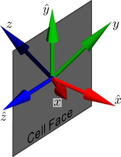
As the interest in this subsection is to obtain the convective flux, let us consider a simplified system with only the pseudo-time derivative and the convective flux vectors. Additionally, consider a rotated coordinate system $\left(\hat{x},\hat{y},\hat{z}\right)$, as shown schematically in Fig. 3, where $\hat{x}$ is the direction normal to the face and $\hat{y}$ and $\hat{z}$ are tangential to the face. In such a coordinate system, only the $\hat{x}$-split three-dimensional governing equations are needed for calculation of convective flux, as the other two flux components will not contribute in the finite volume flux computation. Thus, to compute the convective flux using a Riemann solver the following simplified system of governing equations is sufficient,

$$\frac{\partial\mathbf{\hat{U}}}{\partial\tau}+\frac{\partial\mathbf{\hat{F}}}{\partial\hat{x}}=0\ ,$$ (25)

where, $\mathbf{\hat{F}}=\mathbf{F}\left(\mathbf{\hat{U}}\right)$ and $\mathbf{\hat{U}}=T\,\mathbf{U}$, with the expression for $\mathbf{U}$ same as in equation (1). The transformation matrix $T$ can be obtained to be,

$$T=\left[\begin{array}[]{ccccc}1&0&0&0&0\\ 0&n_{x}&n_{y}&n_{z}&0\\ 0&t_{1x}&t_{1y}&t_{1z}&0\\ 0&t_{2x}&t_{2y}&t_{2z}&0\\ 0&0&0&0&1\end{array}\right]\ ,$$ (26)

where, $\hat{n}=\left(n_{x},n_{y},n_{z}\right)$ is the unit vector normal to the face, pointing from left state to right state (along $\hat{x}$ direction), and, $\hat{t}_{1}=\left(t_{1x},t_{1y},t_{1z}\right)$ and $\hat{t}_{2}=\left(t_{2x},t_{2y},t_{2z}\right)$ are unit orthogonal vectors tangent to the face. The transformed conservative variable vector, $\mathbf{\hat{U}}$, can be written as,

$$\mathbf{\hat{U}}=\left[\begin{array}[]{c}p/\beta\\ \rho\,\left(u\,n_{x}+v\,n_{y}+w\,n_{z}\right)\\ \rho\,\left(u\,t_{1x}+v\,t_{1y}+w\,t_{1z}\right)\\ \rho\,\left(u\,t_{2x}+v\,t_{2y}+w\,t_{2z}\right)\\ C\end{array}\right]=\left[\begin{array}[]{c}p/\beta\\ \rho\,\hat{u}\\ \rho\,\hat{v}\\ \rho\,\hat{w}\\ C\end{array}\right]\ ,$$

where, $\hat{u}=u\,n_{x}+v\,n_{y}+w\,n_{z}$; $\hat{v}=u\,t_{1x}+v\,t_{1y}+w\,t_{1z}$ and $\hat{w}=u\,t_{2x}+v\,t_{2y}+w\,t_{2z}$. The Riemann solver for calculation of convective flux takes the left and the right states at the face, $\left(\mathbf{\hat{U}}_{L},\mathbf{\hat{U}}_{R}\right)$, as inputs and returns the flux through the face, $\mathbf{\hat{F}}_{f}$ as an output.

$$\mathbf{\hat{F}}_{f}=\mathbf{F}_{f}\left(\mathbf{\hat{U}}_{L},\mathbf{\hat{U}}_{R}\right)\ ,$$ (27)

where, $\mathbf{\hat{F}}_{f}$ is the Riemann flux at the cell face. The two initial states, $\left(\mathbf{\hat{U}}_{L},\mathbf{\hat{U}}_{R}\right)$, at the cell face, evolve over pseudo-time, $\tau$, into multiple solution states spreading out in space and time, as shown in Fig. 4. These solution states are separated by discontinuities across the waves. The speeds at which the waves move are associated with the eigenvalues of the Jacobian, $\partial\mathbf{\hat{F}}/\partial\mathbf{\hat{U}}$, which can be calculated to be,

$$\frac{\partial\mathbf{\hat{F}}}{\partial\mathbf{\hat{U}}}=\left[\begin{array}[]{ccccc}0&1/\rho&0&0&\left(\rho_{2}-\rho_{1}\right)\,\hat{u}/\rho\\ \beta&2\,\hat{u}&0&0&\left(\rho_{2}-\rho_{1}\right)\,\hat{u}^{2}\\ 0&\hat{v}&\hat{u}&0&\left(\rho_{2}-\rho_{1}\right)\,\hat{u}\,\hat{v}\\ 0&\hat{w}&0&\hat{u}&\left(\rho_{2}-\rho_{1}\right)\,\hat{u}\,\hat{w}\\ 0&C/\rho&0&0&\rho_{2}\,\hat{u}/\rho\end{array}\right]$$ (28)

The eigenvalues of the Jacobian can be calculated to be,

$$\lambda=\left[\hat{u}_{C}-a,\hat{u},\hat{u},\hat{u},\hat{u}_{C}+a\right]$$ (29)

where,

$$\hat{u}_{C}=\frac{\left(\rho+\rho_{2}\right)\,\hat{u}}{2\,\rho}=\frac{\hat{u}}{2}\left(1+\frac{\rho_{2}}{\rho}\right);\quad a=\sqrt{\hat{u}_{C}^{2}+\beta/\rho}\ .$$ (30)

The right eigenvectors of the Jacobian, written as columns of a matrix, are,

$$R_{ev}=\left[\begin{array}[]{ccccc}1&0&0&0&1\\ \frac{\rho\,\lambda_{1}\left(\hat{u}-\lambda_{4}\right)}{\lambda_{1}-\hat{u}}&0&0&1&\frac{\rho\,\lambda_{4}\,\left(\hat{u}-\lambda_{1}\right)}{\lambda_{4}-\hat{u}}\\ \frac{\rho\,\hat{v}\,\lambda_{1}}{\lambda_{1}-\hat{u}}&1&0&0&\frac{\rho\,\hat{v}\,\lambda_{4}}{\lambda_{4}-\hat{u}}\\ \frac{\rho\,\hat{w}\,\lambda_{1}}{\lambda_{1}-\hat{u}}&0&1&0&\frac{\rho\,\hat{w}\,\lambda_{4}}{\lambda_{4}-\hat{u}}\\ \frac{C\,\lambda_{1}}{\lambda_{1}-\hat{u}}&0&0&\frac{1}{\left(\rho_{1}-\rho_{2}\right)\,\hat{u}}&\frac{C\,\lambda_{4}}{\lambda_{4}-\hat{u}}\end{array}\right]\ .$$ (31)

There are five waves corresponding to each of the eigenvalues, however, since three of the eigenvalues are repeating, it will result in four distinct states separated by three waves as shown in Fig. 4. The solution states are denoted by $\mathbf{\hat{U}}_{L}$, $\mathbf{\hat{U}}_{*L}$, $\mathbf{\hat{U}}_{*R}$, $\mathbf{\hat{U}}_{R}$ and the wave speeds are denoted by $S_{L}$, $S_{*}$ and $S_{R}$.

Fig. 4: Schematic diagram depicting the wave structure of a Riemann solver with three distinct waves.

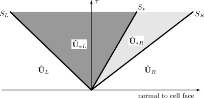
This results in the following definition of flux depending on the wave speeds,

$$\mathbf{\hat{F}}_{f}=\begin{cases}\mathbf{\hat{F}}_{L}&S_{L}\geq 0\\ \mathbf{\hat{F}}_{*L}&S_{L}\leq 0\leq S_{*}\\ \mathbf{\hat{F}}_{*R}&S_{*}\leq 0\leq S_{R}\\ \mathbf{\hat{F}}_{R}&S_{R}\leq 0\end{cases}$$ (32)

where,

$$\mathbf{\hat{F}}_{L}=\mathbf{F}\left(\mathbf{\hat{U}}_{L}\right)\ ;\quad\mathbf{\hat{F}}_{R}=\mathbf{F}\left(\mathbf{\hat{U}}_{R}\right)\ ;$$ (33)

and using the Rankine-Hugoniot jump conditions across the left and right wave,

$$\mathbf{\hat{F}}_{*L}=\mathbf{\hat{F}}_{L}+S_{L}\left(\mathbf{\hat{U}}_{*L}-\mathbf{\hat{U}}_{L}\right)\ ;$$ (34)

$$\mathbf{\hat{F}}_{*R}=\mathbf{\hat{F}}_{R}+S_{R}\left(\mathbf{\hat{U}}_{*R}-\mathbf{\hat{U}}_{R}\right)\ .$$ (35)

The intermediate states, $\mathbf{\hat{U}}_{*L}$, $\mathbf{\hat{U}}_{*R}$, and the intermediate wave speed, $S_{*}$, can be calculated by using the Rankine-Hugoniot jump conditions and imposing additional conditions obtained from generalized Riemann invariant analysis. After a considerable amount of mathematical rigor all the above unknowns can be estimated. All the expressions necessary for calculation of convective flux are concisely given below.

$$\mathbf{\hat{F}}_{L}=\mathbf{F}\left(\hat{\mathbf{U}}_{L}\right)=\left[\begin{array}[]{c}\hat{u}\\ \rho\,\hat{u}^{2}+p\\ \rho\,\hat{u}\,\hat{v}\\ \rho\,\hat{u}\,\hat{w}\\ C\,\hat{u}\end{array}\right]_{L};\qquad\mathbf{\hat{F}}_{R}=\mathbf{F}\left(\mathbf{\hat{U}}_{R}\right)=\left[\begin{array}[]{c}\hat{u}\\ \rho\,\hat{u}^{2}+p\\ \rho\,\hat{u}\,\hat{v}\\ \rho\,\hat{u}\,\hat{w}\\ C\,\hat{u}\end{array}\right]_{R}$$ (36)

$$\boxed{\rho_{L}=\left(\rho_{1}-\rho_{2}\right)\left[C\right]_{L}+\rho_{2}}\qquad\boxed{\rho_{R}=\left(\rho_{1}-\rho_{2}\right)\left[C\right]_{R}+\rho_{2}}$$ (37)

$$\hat{u}_{CL}=\left[\hat{u}\right]_{L}\,\frac{\left(\rho_{L}+\rho_{2}\right)}{2\,\rho_{L}}\qquad\hat{u}_{CR}=\left[\hat{u}\right]_{R}\,\frac{\left(\rho_{R}+\rho_{2}\right)}{2\,\rho_{R}}$$ (38)

$$a_{L}=\sqrt{\hat{u}_{CL}^{2}+\beta/\rho_{L}};\qquad a_{R}=\sqrt{\hat{u}_{CR}^{2}+\beta/\rho_{R}}$$ (39)

$$\boxed{S_{L}=\min\left(\hat{u}_{CL}-a_{L},\hat{u}_{CR}-a_{R}\right)}\qquad\boxed{S_{R}=\max\left(\hat{u}_{CL}+a_{L},\hat{u}_{CR}+a_{R}\right)}$$ (40)

$$\boxed{\left[p/\beta\right]_{*L}=\left[p/\beta\right]_{*R}=\left[p/\beta\right]_{*}=\frac{\left[\hat{u}\right]_{L}-\left[\hat{u}\right]_{R}+S_{R}\left[p/\beta\right]_{R}-S_{L}\left[p/\beta\right]_{L}}{S_{R}-S_{L}}}$$ (41)

$$\boxed{\hat{u}_{*L}=\hat{u}_{*R}=\hat{u}_{*}=S_{*}=\frac{S_{R}\left[\rho\,\hat{u}\right]_{R}-S_{L}\left[\rho\,\hat{u}\right]_{L}-\left[\rho\,\hat{u}^{2}+p\right]_{R}+\left[\rho\,\hat{u}^{2}+p\right]_{L}}{S_{R}\rho_{R}-S_{L}\rho_{L}-\left(\rho_{1}-\rho_{2}\right)\left(\left[C\,\hat{u}\right]_{R}-\left[C\,\hat{u}\right]_{L}\right)}}$$ (42)

$$\boxed{\left[C\right]_{*L}=\frac{S_{L}\left[C\right]_{L}-\left[C\,\hat{u}\right]_{L}}{S_{L}-S_{*}}}\qquad\boxed{\left[C\right]_{*R}=\frac{S_{R}\left[C\right]_{R}-\left[C\,\hat{u}\right]_{R}}{S_{R}-S_{*}}}$$ (43)

$$\boxed{\rho_{*L}=\left(\rho_{1}-\rho_{2}\right)\left[C\right]_{*L}+\rho_{2}}\qquad\boxed{\rho_{*R}=\left(\rho_{1}-\rho_{2}\right)\left[C\right]_{*R}+\rho_{2}}$$ (44)

$$\boxed{\left[\rho\,\hat{u}\right]_{*L}=\rho_{*L}\hat{u}_{*}}\qquad\boxed{\left[\rho\,\hat{u}\right]_{*R}=\rho_{*R}\hat{u}_{*}}$$ (45)

$$\boxed{\left[\rho\,\hat{v}\right]_{*L}=\frac{S_{L}\left[\rho\,\hat{v}\right]_{L}-\left[\rho\,\hat{u}\,\hat{v}\right]_{L}}{S_{L}-S_{*}}}\qquad\boxed{\left[\rho\,\hat{v}\right]_{*R}=\frac{S_{R}\left[\rho\,\hat{v}\right]_{R}-\left[\rho\,\hat{u}\,\hat{v}\right]_{R}}{S_{R}-S_{*}}}$$ (46)

$$\boxed{\left[\rho\,\hat{w}\right]_{*L}=\frac{S_{L}\left[\rho\,\hat{w}\right]_{L}-\left[\rho\,\hat{u}\,\hat{w}\right]_{L}}{S_{L}-S_{*}}}\qquad\boxed{\left[\rho\,\hat{w}\right]_{*R}=\frac{S_{R}\left[\rho\,\hat{w}\right]_{R}-\left[\rho\,\hat{u}\,\hat{w}\right]_{R}}{S_{R}-S_{*}}}$$ (47)

The terms in square brackets $\left[\ \right]$ indicate either conservative variables or convective flux variables, which are stored in corresponding vectors and can be used without additional computation. The intermediate states are obtained by assembling the above terms as,

$$\mathbf{U}_{*L}=\left[\begin{array}[]{c}p/\beta\\ \rho\,\hat{u}\\ \rho\,\hat{v}\\ \rho\,\hat{w}\\ C\end{array}\right]_{*L}\qquad\mathbf{U}_{*R}=\left[\begin{array}[]{c}p/\beta\\ \rho\,\hat{u}\\ \rho\,\hat{v}\\ \rho\,\hat{w}\\ C\end{array}\right]_{*R}\ .$$ (48)

The convective flux in the rotated coordinate system can then be computed using equations (32), (34) and (35).

Finally, to compute the required flux in the finite volume formulation in the original coordinate system $\left(x,y,z\right)$, the inverse transform can be applied,

$$\mathbf{F}\,n_{x}+\mathbf{G}\,n_{y}+\mathbf{H}\,n_{z}=T^{-1}\mathbf{\hat{F}}_{f}\ .$$ (49)

Since the transformation matrix, $T$, is orthonormal, its inverse can be calculated by simply transposing the matrix,

$$T^{-1}=\left[\begin{array}[]{ccccc}1&0&0&0&0\\ 0&n_{x}&t_{1x}&t_{2x}&0\\ 0&n_{y}&t_{1y}&t_{2y}&0\\ 0&n_{z}&t_{1z}&t_{2z}&0\\ 0&0&0&0&1\end{array}\right]\ .$$ (50)

The HLLC-VOF-M Riemann solver can be used for solving 2D and 3D problems, using structured or unstructured mixed cells, without any modifications in the formulation.

3.4 Interface compression

Approximate Riemann solvers inherently introduce some numerical dissipation to ensure stability. This is acceptable in case of compressible fluid flows, where Riemann solvers are extensively used, as the governing equations itself aids compression of discontinuities, such as shocks, to produce correct solutions. The passively advected volume fraction, on the other hand, will keep spreading out the discontinuous volume fraction at the interface, if not corrected artificially. To ensure sharp interfaces, an interface compression term, $\nabla\cdot\mathbf{F}_{c}$, is added to the governing equations (1). This technique is borrowed from [21], which is also implemented in OpenFOAM [23], and modified based on later advancements in the technique [24, 25]. The compression term can be written as,

$$\nabla\cdot\mathbf{F}_{c}=\left[0,0,0,0,\nabla\cdot\vec{V}_{c}\,\left(1-C\right)\,C\right]^{T}\ .$$

The resulting VOF equation becomes,

$$\frac{\partial C}{\partial\tau}+\frac{\partial C}{\partial t}+\nabla\cdot\left(\vec{V}\,C+\vec{V}_{c}\,\left(1-C\right)\,C\right)=0\ ,$$ (51)

where, $\vec{V}=\left(u,v,w\right)$ is the velocity field of the fluids and $\vec{V}_{c}$ is the compressive velocity field. The term $\left(1-C\right)\,C$, ensures that the interface compression is active only near the interface.

The advection part of the flux, due to the term $\vec{V}\,C$, is calculated by the HLLC-VOF-M Riemann solver, therefore only the compressive part of the flux, due to the term $\vec{V}_{c}\,\left(1-C\right)\,C$, needs to be computed. The remaining equation, without $\vec{V}\,C$, can be viewed like an advection equation of $C$, with $\vec{V}_{c}\,\left(1-C\right)$ as the advection velocity field. The required compressive flux can therefore be calculated using a simple scalar upwind solver using the left and right states of volume fraction, $C_{L}$ and $C_{R}$,

$$F_{fc}=\begin{cases}\lambda_{c}\,C_{L}&\lambda_{c}>0\ ;\\ \lambda_{c}\,C_{R}&\text{otherwise}\ .\end{cases}$$ (52)

The wave speed is calculated as $\lambda_{c}=\left(1-C_{f}\right)\vec{V}_{c}\cdot\hat{n}$. The volume fraction at the cell face is denoted as $C_{f}$. The compressive velocity field is computed based on literature [21] as,

$$\vec{V}_{c}=\zeta\,\eta\,\left|\vec{V}_{f}\cdot\hat{n}\right|\hat{n}_{i}\ ,$$ (53)

where, $\zeta$ is the compressive coefficient which can be chosen in the range of 0 to 1. In this work, a value of $\zeta=0.3$ is used. $\eta$ is called the dynamic interface compression coefficient which is given as $\eta=\sqrt{\left|\hat{n}\cdot\hat{n}_{i}\right|}$. The unit vector normal to cell face is $\hat{n}$ and $\hat{n}_{i}$ is the unit vector perpendicular to fluid interface, calculated as,

$$\hat{n}_{i}=\begin{cases}\nabla C_{f}/\left|\nabla C_{f}\right|&\text{if}\ \left|\nabla C_{f}\right|>10^{-6}\ ,\\ 0&\text{otherwise}\ ,\end{cases}$$ (54)

to avoid division by zero. The velocity at the cell face, $\vec{V}_{f}$; the volume fraction at the cell face, $C_{f}$; and the gradient of volume fraction at the cell face, $\nabla C_{f}$, are calculated as a part of viscous flux calculation (explained in section 3.5) and are reused for interface compression. The value obtained by equation (52) is simply added to the fifth component of flux obtained by the HLLC-VOF-M Riemann solver (or HLL Riemann solver, when used for comparison) to avoid smearing of the interface.

3.5 Calculation of viscous flux

In the finite volume discretization, the viscous flux needs to be calculated at the cell faces. Hence, the velocity gradients, $\nabla V$, and the dynamic coefficient of viscosity, $\mu$, need to be computed at the cell faces. The velocity gradients can be written as,

$$\nabla V=\left[\begin{array}[]{ccc}\partial u/\partial x&\partial u/\partial y&\partial u/\partial z\\ \partial v/\partial x&\partial v/\partial y&\partial v/\partial z\\ \partial w/\partial x&\partial w/\partial y&\partial w/\partial z\end{array}\right]\ .$$ (55)

For numerical computation of derivatives at the face, cell values in the vicinity of the face are needed. Consider the cell $i$ shown in Fig. 5. The set of neighbors of a face, say $j=1$, is constructed by collecting the neighbors of all the nodes of the face. In the example shown in Fig. 5, this will result in a set of 6 neighbors i.e. cells $n=1\dots 5$ and cell $i$. Here a quadrilateral cell is considered, however the same strategy can be followed for all types of cells, in two- and three-dimensions.

Fig. 5: An example of face neighbors for numerical calculation of gradients at the cell face $j=1$

In a finite volume formulation, as we know the cell averaged values of the conservative variables, the required derivatives of velocity are calculated in two steps. The first step is to compute the gradients of the conservative variables at the face; and the second step is to convert the gradients of conservative variables to gradients of velocity by using the Jacobian of transformation. The gradients of the conservative variables are calculated by using a truncated Taylor series. Consider a variable, $\xi$, to be a component of the conservative variable vector $\mathbf{U}$. A truncated Taylor series to obtain a linear approximation of $\xi$ can be written as,

$$\xi_{n}=\xi_{j}+\left.\frac{\partial\xi}{\partial x}\right|_{j}\Delta x_{n}+\left.\frac{\partial\xi}{\partial y}\right|_{j}\Delta y_{n}+\left.\frac{\partial\xi}{\partial z}\right|_{j}\Delta z_{n}\ ,$$ (56)

where, the derivatives are evaluated at the centroid of face $j$. $\left(\Delta x_{n},\Delta y_{n},\Delta z_{n}\right)$ is the vector from the centroid of face $j$ to the centroid of neighbor cell $n$. Writing the above equation for all the neighbors, $n=1,2\dots N$, of a face will result in the following system:

$$\underbrace{\left[\begin{array}[]{cccc}1&\Delta x_{1}&\Delta y_{1}&\Delta z_{1}\\ 1&\Delta x_{2}&\Delta y_{2}&\Delta z_{2}\\ \vdots&\vdots&\vdots&\vdots\\ 1&\Delta x_{N}&\Delta y_{N}&\Delta z_{N}\end{array}\right]}_{S}\cdot\underbrace{\left[\begin{array}[]{c}\xi\\ \partial\xi/\partial x\\ \partial\xi/\partial y\\ \partial\xi/\partial z\end{array}\right]_{j}}_{\xi_{j}^{\prime}}=\underbrace{\left[\begin{array}[]{c}\xi_{1}\\ \xi_{2}\\ \vdots\\ \xi_{N}\end{array}\right]}_{\xi_{n}}\ .$$ (57)

The equations are weighted using inverse-distance based weights, $w_{n}=1/\left\|\Delta r_{n}\right\|$, where $\left\|\Delta r_{n}\right\|=\sqrt{\Delta x_{n}^{2}+\Delta y_{n}^{2}+\Delta z_{n}^{2}}$. The system of equations with weights can be written as,

$$W\,S\,\xi_{j}^{\prime}=W\,\xi_{n}\ ,$$ (58)

with $W=\text{diag}\left(w_{1},w_{2}\dots w_{N}\right)$. This results in a tall system of equations with four unknowns, $\xi$, $\partial\xi/\partial x$, $\partial\xi/\partial y$ and $\partial\xi/\partial z$ at the centroid of face $j$. The system is solved by using singular value decomposition (SVD) method using an open source mathematical library [36].

The above procedure can be followed for each component of the conservative variable vector, $\mathbf{U}$, to obtain its value and gradient at the cell face. The gradients of conservative variables at a face $j$, can be packed together as,

$$\nabla\mathbf{U}_{j}=\left[\begin{array}[]{ccc}\partial U_{1}/\partial x&\partial U_{1}/\partial y&\partial U_{1}/\partial z\\ \partial U_{2}/\partial x&\partial U_{2}/\partial y&\partial U_{2}/\partial z\\ \partial U_{3}/\partial x&\partial U_{3}/\partial y&\partial U_{3}/\partial z\\ \partial U_{4}/\partial x&\partial U_{4}/\partial y&\partial U_{4}/\partial z\\ \partial U_{5}/\partial x&\partial U_{5}/\partial y&\partial U_{5}/\partial z\end{array}\right]\ ,$$ (59)

where, $U_{1}=p/\beta$, $U_{2}=\rho\,u$, $U_{3}=\rho\,v$, $U_{4}=\rho\,w$, $U_{5}=C$.

Once the gradients of the conservative variables at the cell face are computed, the second step is to calculate the velocity gradients by using the transformation,

$$\nabla V_{j}=J\,\nabla\mathbf{U}_{j}\ ,$$ (60)

where $J$ is the Jacobian, obtained as,

$$J=\frac{\partial V}{\partial\mathbf{U}}=\left[\begin{array}[]{ccccc}0&1/\rho_{j}&0&0&\frac{\left(\rho_{2}-\rho_{1}\right)u_{j}}{\rho_{j}}\\ 0&0&1/\rho_{j}&0&\frac{\left(\rho_{2}-\rho_{1}\right)v_{j}}{\rho_{j}}\\ 0&0&0&1/\rho_{j}&\frac{\left(\rho_{2}-\rho_{1}\right)w_{j}}{\rho_{j}}\end{array}\right]\ .$$ (61)

As a part of the solution of system (58), the interpolated values of conservative variables, $\left(\rho u\right)_{j}$, $\left(\rho v\right)_{j}$, $\left(\rho w\right)_{j}$ and $C_{j}$, are also obtained at the cell face. The density, $\rho_{j}$, at the cell face can be calculated using equation (2). The velocity components at the cell face can be calculated as,

$$u_{j}=\left(\rho u\right)_{j}/\rho_{j},\quad v_{j}=\left(\rho v\right)_{j}/\rho_{j},\quad w_{j}=\left(\rho w\right)_{j}/\rho_{j}\ ,$$ (62)

which can be used for calculation of the Jacobian, $J$. The value of the coefficient of dynamic viscosity, $\mu_{j}$, at the cell face can be calculated using equation (3). The viscous flux can be calculated using the obtained gradients of velocity and coefficient of dynamic viscosity.

3.6 Calculation of surface tension flux

Surface tension is a force which acts only at the interface between two fluids, which is a result of intermolecular forces. This force acts in such a way so as to minimize the surface area of the interface. The magnitude of the resultant force is proportional to surface tension coefficient, $\sigma$, corresponding to the fluids. The value of $\sigma$ can be obtained experimentally for different fluid combinations from literature [39]. This force is commonly modeled in numerical simulations, using interface capturing methods, by the continuum surface force (CSF) [33] or the continuum surface stress (CSS) [40] models. In this work, the CSS method is used for modeling surface tension as it does not require explicit calculation of interface curvature. Also, based on numerical experiments it was observed by [40], that the CSS model does not require smoothening of VOF function. Hence, it is very straightforward and quite natural to combine the CSS model within the VOF framework in a conservative finite volume formulation. The CSS model describes the surface tension force in a momentum equation as,

$$\mathbf{F_{s}}=\sigma\,\left(\left|\nabla C\right|\ I-\frac{\nabla C\otimes\nabla C}{\left|\nabla C\right|}\right)\ ,$$ (63)

where, $\sigma$ is the surface tension coefficient, $\nabla C$ is the gradient of volume fraction, $\left|\nabla C\right|$ is the magnitude of the gradient vector and $I$ is a $3\times 3$ identity matrix. The surface tension force in the governing equations (1) therefore becomes,

$$\nabla\cdot\mathbf{T}=\left[\begin{array}[]{c}0\\ \nabla\cdot\mathbf{F_{s}}\\ 0\end{array}\right]\ .$$

The surface tension force is set to zero away from the interface, explicitly, when the value of $\left|\nabla C\right|<10^{-6}$ to avoid division by zero. The tensor $\nabla C\otimes\nabla C$ is defined as,

$$\nabla C\otimes\nabla C=\nabla C^{T}\nabla C=\left[\begin{array}[]{ccc}\left(\frac{\partial C}{\partial x}\right)^{2}&\frac{\partial C}{\partial x}\frac{\partial C}{\partial y}&\frac{\partial C}{\partial x}\frac{\partial C}{\partial z}\\ \frac{\partial C}{\partial x}\frac{\partial C}{\partial y}&\left(\frac{\partial C}{\partial y}\right)^{2}&\frac{\partial C}{\partial y}\frac{\partial C}{\partial z}\\ \frac{\partial C}{\partial x}\frac{\partial C}{\partial z}&\frac{\partial C}{\partial y}\frac{\partial C}{\partial z}&\left(\frac{\partial C}{\partial z}\right)^{2}\end{array}\right]\ .$$ (64)

For incorporating the CSS model into finite volume formulation, the value of $\mathbf{F_{s}}$ has to be computed at the cell face. The gradients at the face,$\nabla\mathbf{U}_{j}$, are computed during calculation of viscous flux, which is described in sub-section 3.5. The gradient of volume fraction for a face $j$ is calculated as,

$$\nabla C_{j}^{T}=J\,\nabla\mathbf{U}_{j}\ ,$$ (65)

where $J$ can be obtained to be,

$$J=\frac{\partial C}{\partial\mathbf{U}}=\left[\begin{array}[]{ccccc}0&0&0&0&1\end{array}\right]\ .$$ (66)

3.7 Treatment of source term

The source term in the finite volume formulation is given by $\Omega_{P}\,\overline{\mathbf{S}}$, with $\mathbf{\overline{S}}=\left[0,\overline{\rho}\,g_{x},\overline{\rho}\,g_{y},\overline{\rho}\,g_{z},0\right]^{T}$ and $\Omega_{P}$ is the volume of the cell. The average value of the density, $\overline{\rho}$, can be computed simply by using equation (2) and substituting the average value of volume fraction, $\overline{C}$, which is available in the finite volume formulation.

3.8 Initial conditions

An accurate calculation of the initial cell-averaged values of conservative variables is important in two-phase flow problems, as the solution is sensitive to initial position of the fluid interface. To obtain the initial cell-averaged values, an integration of the initial distribution needs to be computed over each cell. A numerical integration is carried out, for each cell, by subdividing the cell into smaller parts and then performing a Riemann sum. In case of quadrilateral (and hexahedral) cells, the cell is divided by using transfinite interpolation with 20 divisions (4 divisions for hexahedral) along each computational coordinate direction. This results in $20\times 20$ sub-quadrilaterals ($4\times 4\times 4$ sub-hexahedrals) per cell. In case of triangular cells, the sub-triangles are generated by using 5 levels of recursive sub-division with each level diving a triangle into 4 equal sub-triangles. This results in $1024$ sub-triangles per cell.

3.9 Boundary conditions

The boundary conditions are implemented using ghost cells (also known as dummy cells). The ghost cells are additional finite volume cells added outside the computational domain so that gradients at the boundary can be specified or computed. There are three types of boundary conditions used in this work: the stationary slip wall (also called inviscid wall), stationary no-slip wall (also called viscous wall) and symmetry boundary condition. In all these boundary conditions the normal component of velocity is zero, therefore the convective flux is given by $\left[0,p\,n_{x},p\,n_{y},p\,n_{z},0\right]^{T}$. The calculation of viscous and the surface tension flux at the boundary depend on the gradients of variables at the boundary face, therefore the ghost cells have to be set appropriately. In case of slip wall boundary, the inside velocity vector is mirrored about the boundary plane, while the pressure and volume fraction are extrapolated using corresponding values and gradients from the inside cell. In case of no-slip boundary, the negative of velocity vector is copied to the ghost cell, while the pressure and volume fraction are extrapolated. In case of symmetry, the inside velocity vector is mirrored about the boundary plane, while the pressure and volume fraction are copied as it is to the ghost cell.

4 The Algorithm

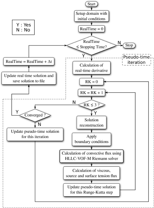
The Navier-Stokes equations are written using artificial compressibility formulation and combined with the VOF equation to simulate transient two-phase flows. A dual-time stepping algorithm is used to obtain a time-accurate solution of the flow field. The dual-time stepping method allows for implicit treatment of real-time variables, and therefore the real-time step size is restricted only by the physics of the flow. In the dual time stepping approach, the outer loop advances the real-time variables, $\mathbf{W}$, in real-time, $t$. The inner loop iterates in pseudo-time, $\tau$, and continues until the solution converges to a time accurate solution, as the residual drops below acceptable limits (which is chosen as $10^{-3}$ in this work). During the pseudo-time iterations, as the solution evolves, the latest solution is used for evaluating the total residual. The total residual is computed by summing up the convective, interface compression, viscous, surface tension and the source residual. The convective part of the residual is computed using the HLLC-VOF-M Riemann solver, introduced in this paper. A flowchart of the complete algorithm is displayed in Fig. 6.

Fig. 6: Flowchart of the complete algorithm

5 Results and discussion

To test the efficacy and practical applicability of the HLLC-VOF-M convective flux solver, several two-dimensional problems are solved using structured and unstructured mesh. Also, a three-dimensional problem involving complex merging of interfaces is solved to demonstrate the extensibility and robustness of the solver. The results are compared with theoretical, experimental and numerical results available in literature. In all the problems the artificial compressibility parameter, $\beta$, is chosen to be $1000$. The velocity field of the flow is displayed in some figures, using scaled arrows. The scaling of these arrows is based on the largest velocity magnitude in the complete domain at the time instant. The fluid interface is displayed by plotting two levels at 0.3 and 0.7, in all the two-dimensional contour plots. In three-dimensions, a contour level of 0.5 is used to display the fluid interface.

5.1 Droplet splash

In this problem, a two-dimensional circular water droplet is placed over bulk water body separated by air. Numerical results of this problem are available in literature [41], where high order pressure-based, projection method is used. The effect of surface tension is not considered in the said paper, hence in this problem the surface tension coefficient is set to zero. The properties of the two fluids considered are water ($\rho_{1}=998\,\text{kg/m}^{3},\mu_{1}=1.002\times 10^{-3}\,\text{Pa-s}$) and air ($\rho_{2}=1.2\,\text{kg/m}^{3},\mu_{2}=1.825\times 10^{-5}\,\text{Pa-s}$). The acceleration due to gravity is $g=\left(0,-9.81,0\right)\,\text{m/s}^{2}$. The domain is of size $0.007\,\text{m}\times 0.014\,\text{m}$ with water filled up to $0.0088\,\text{m}$. The water droplet is placed above the water surface with its center at $\left(0.0035\,\text{m},\ 0.0105\,\text{m}\right)$ and having a diameter of $2.8\times 10^{-3}\,\text{m}$. The domain is discretized using a Cartesian mesh of size $80\times 160$. The initial velocity and pressure in the entire domain is zero. The problem is solved up to a time of $t=0.025\,\text{s}$ using steps of $\Delta t=10^{-5}\,\text{s}$. The initial distribution of volume fraction along with the snapshots of the solution at various other time steps (same as [41]) using HLLC-VOF-M and HLL are shown in Fig. 7 and Fig. 8 respectively. It can be seen that the results obtained by the non-contact capturing HLL solver produces excessive numerical dissipation and the tiny air bubbles trapped inside the water are not captured by the solution. On the other hand, the results obtained using HLLC-VOF-M solver agree very well with the results from the literature [41].

$t=0.0\,\text{s}$
	$t=0.00677\,\text{s}$
	$t=0.00980\,\text{s}$
	$t=0.01220\,\text{s}$
	$t=0.01485\,\text{s}$	$t=0.01781\,\text{s}$	$t=0.01995\,\text{s}$	$t=0.02146\,\text{s}$

Fig. 7: Snapshots of the drop splash problem at various time levels, using HLLC-VOF-M solver.

$t=0.0\,\text{s}$
	$t=0.00677\,\text{s}$
	$t=0.00980\,\text{s}$
	$t=0.01220\,\text{s}$
	$t=0.01485\,\text{s}$	$t=0.01781\,\text{s}$	$t=0.01995\,\text{s}$	$t=0.02146\,\text{s}$

Fig. 8: Snapshots of the drop splash problem at various time levels, using HLL solver.

5.2 Three-dimensional non-axisymmetric merging of bubbles

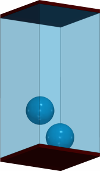
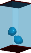
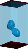
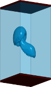
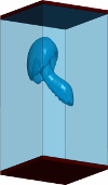
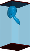
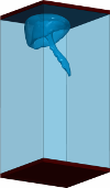
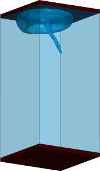
In this problem, two spherical bubbles are placed slightly offset to one another in a tank of size $1\,\text{m}\times 2\mbox{\,\text{m}}\times 1\,\text{m}$. The diameter of the bubbles is $0.4\,\text{m}$. The lower bubble is centered at $\left(0.6\,\text{m},0.25\,\text{m},0.6\,\text{m}\right)$; and the upper bubble is centered at $\left(0.4\,\text{m},0.65\,\text{m},0.4\,\text{m}\right)$, measured from the bottom corner. Due to buoyancy the bubbles start moving up, and merge together as time evolves. A similar problem is solved numerically, in literature [42], using the advancing front method.

The bubbles and the outer fluid can be characterized by using the Eötvös number $Eo=\rho_{1}\,g\,d_{e}^{2}/\sigma$, the Morton number $M=g\,\mu_{1}^{4}/\left(\rho_{1}\,\sigma\right)$, and the ratio of fluid properties $\rho_{1}/\rho_{2}$ and $\mu_{1}/\mu_{2}$. Subscript 1 is used for heavier outer fluid and subscript 2 is used for the fluid contained inside the bubbles. The acceleration due to gravity in the downward direction is chosen as, $g=1\,\text{m/s}^{2}$; the density of the outer fluid is chosen as, $\rho_{1}=1\,\text{kg/m}^{3}$; and the effective diameter of the bubbles is $d_{e}=0.4\,\text{m}$. The simulation is performed for $Eo=50$, $M=1$, $\rho_{1}/\rho_{2}=20$ and $\mu_{1}/\mu_{2}=26$. The remaining fluid properties can be easily evaluated using the above equations. The domain is discretized using a mesh of $32\times 64\times 32$ cells. The pressure and velocity are initialized to zero in the entire domain. All the boundaries of the domain are set as slip-walls. The simulation is carried out for a time duration of $t=5\,\text{s}$ with a time step of $\Delta t=0.001\,\text{s}$. Various snapshots of the solution at different times of evolution are shown in Fig. 9. The solutions from literature [42] are visually similar to the solutions displayed in Fig. 9.

$t=0.0\,\text{s}$
	$t=0.2\,\text{s}$
	$t=0.4\,\text{s}$
	$t=0.6\,\text{s}$
	$t=0.8\,\text{s}$	$t=1.0\,\text{s}$	$t=1.2\,\text{s}$	$t=1.4\,\text{s}$

Fig. 9: Snapshots of two non-axisymmetric rising bubbles at different times, computed using HLLC-VOF-M Riemann solver. Mesh = $32\times 64\times 32$ cells, $Eo=50$, $M=1$, $\rho_{1}/\rho_{2}=20$ and $\mu_{1}/\mu_{2}=26$.

6 Conclusion

An improved HLLC-type Riemann solver is developed for three-dimensional, incompressible two-phase fluid flow. The flow is modeled using the artificial compressibility formulation and volume of fluid method. The convective flux is derived for the system of governing equations using the Rankine-Hugoniot jump conditions. The generalized Riemann invariant analysis is used to apply the necessary additional constraints. The convective flux computation using an upwind type solver inherently introduces numerical dissipation, which causes smearing of the fluid interface. Therefore, an interface compression mechanism is adopted to overcome the unphysical dissipation effectively. The viscous flux is computed using weighted least squares, the surface tension is computed using the CSS model, and the source term is computed using the cell average values. The solver is generic and can be used to solve incompressible two-phase flow problems using structured and unstructured meshes in two- and three-dimensions, without any modifications. The new Riemann solver is found to be robust and performs well in all the selected test problems with a single chosen value of artificial compressibility parameter, $\beta$, unlike our previous formulation [14], where the value of $\beta$ was determined based on trial-and-error. Various two- and three-dimensional test problems are solved on different mesh types to demonstrate the efficacy and robustness of the new solver.

References

- [1] A. Belov, L. Martinelli, and A. Jameson, “A new implicit algorithm with multigrid for unsteady incompressible flow calculations,” in 33rd Aerospace Sciences Meeting and Exhibit, Aerospace Sciences Meetings, American Institute of Aeronautics and Astronautics, jan 1995.
- [2] P. Tamamidis, G. Zhang, and D. N. Assanis, “Comparison of Pressure-Based and Artificial Compressibility Methods for Solving 3D Steady Incompressible Viscous Flows,” Journal of Computational Physics, vol. 124, no. 1, pp. 1–13, 1996.
- [3] D. Drikakis, O. P. Iliev, and D. P. Vassileva, “A Nonlinear Multigrid Method for the Three-Dimensional Incompressible Navier-Stokes Equations,” Journal of Computational Physics, vol. 146, no. 1, pp. 301–321, 1998.
- [4] A. L. Gaitonde, “A dual-time method for two-dimensional unsteady incompressible flow calculations,” International Journal for Numerical Methods in Engineering, vol. 41, no. 6, pp. 1153–1166, 1998.
- [5] M. T. Manzari, “An explicit finite element algorithm for convection heat transfer problems,” International Journal of Numerical Methods for Heat & Fluid Flow, vol. 9, pp. 860–877, dec 1999.
- [6] Y. Zhao and B. Zhang, “A high-order characteristics upwind FV method for incompressible flow and heat transfer simulation on unstructured grids,” Computer Methods in Applied Mechanics and Engineering, vol. 190, no. 5, pp. 733–756, 2000.
- [7] A. G. Malan, R. W. Lewis, and P. Nithiarasu, “An improved unsteady, unstructured, artificial compressibility, finite volume scheme for viscous incompressible flows: Part I. Theory and implementation,” International Journal for Numerical Methods in Engineering, vol. 54, pp. 695–714, jun 2002.
- [8] J. C. Mandal and A. S. Iyer, “An upwind method for incompressible flow computations using pseudo-compressibility approach,” in 19th AIAA Computational Fluid Dynamics Conference, 2009.
- [9] Y. Zhao, H. Hui Tan, and B. Zhang, “A High-Resolution Characteristics-Based Implicit Dual Time-Stepping VOF Method for Free Surface Flow Simulation on Unstructured Grids,” Journal of Computational Physics, vol. 183, pp. 233–273, Nov. 2002.
- [10] R. R. Nourgaliev, T. N. Dinh, and T. G. Theofanous, “A pseudocompressibility method for the numerical simulation of incompressible multifluid flows,” International Journal of Multiphase Flow, vol. 30, no. 7, pp. 901–937, 2004.
- [11] S. N. Yakovenko and K. C. Chang, “Volume fraction flux approximation in a two-fluid flow,” Thermophysics and Aeromechanics, vol. 15, pp. 169–186, Nov. 2008.
- [12] Y.-Y. Niu and J. R. Edwards, “A simple incompressible flux splitting for sharp free surface capturing,” International Journal for Numerical Methods in Fluids, vol. 69, pp. 1661–1678, jul 2011.
- [13] A. J. Chorin, “A numerical method for solving incompressible viscous flow problems,” Journal of Computational Physics, vol. 2, pp. 12–26, aug 1967.
- [14] S. Bhat and J. Mandal, “Contact preserving Riemann solver for incompressible two-phase flows,” Journal of Computational Physics, vol. 379, pp. 173–191, feb 2019.
- [15] W. G. Price and Y. G. Chen, “A simulation of free surface waves for incompressible two-phase flows using a curvilinear level set formulation,” International Journal for Numerical Methods in Fluids, vol. 51, no. 3, pp. 305–330, 2006.
- [16] A. Yang, S. Chen, L. Yang, and X. Yang, “An upwind finite volume method for incompressible inviscid free surface flows,” Computers & Fluids, vol. 101, pp. 170–182, sep 2014.
- [17] S. Parameswaran and J. Mandal, “A novel Roe solver for incompressible two-phase flow problems,” Journal of Computational Physics, vol. 390, pp. 405–424, aug 2019.
- [18] W. J. Rider and D. B. Kothe, “Reconstructing Volume Tracking,” Journal of Computational Physics, vol. 141, pp. 112–152, 1998.
- [19] M. Rudman, “Volume Tracking Methods for Interfacial Flows Calculations,” International Journal for Numerical Methods in Fluids, vol. 24, pp. 671–691, 1997.
- [20] O. Ubbink and R. I. Issa, “A Method for Capturing Sharp Fluid Interfaces on Arbitrary Meshes,” Journal of Computational Physics, vol. 153, pp. 26–50, 1999.
- [21] H. Rusche, Computational Fluid Dynamics of Dispersed Two-Phase Flows at High Phase Fractions. PhD thesis, Imperial College of Science, Technology & Medicine, 2002.
- [22] P. Cifani, W. Michalek, G. Priems, J. Kuerten, C. van der Geld, and B. Geurts, “A comparison between the surface compression method and an interface reconstruction method for the VOF approach,” Computers & Fluids, vol. 136, pp. 421–435, sep 2016.
- [23] H. Jasak, “OpenFOAM: Open source CFD in research and industry,” International Journal of Naval Architecture and Ocean Engineering, vol. 1, pp. 89–94, dec 2009.
- [24] H. Lee and S. H. Rhee, “A dynamic interface compression method for VOF simulations of high-speed planing watercraft,” Journal of Mechanical Science and Technology, 2015.
- [25] Y. Mehmani, “Wrinkle-Free Interface Compression for Two-Fluid Flows,” nov 2018.
- [26] V. Venkatakrishnan, “Convergence to Steady State Solutions of the Euler Equations on Unstructured Grids with Limiters,” Journal of Computational Physics, vol. 118, pp. 120–130, apr 1995.
- [27] A. Jameson, “Time dependent calculations using multigrid, with applications to unsteady flows past airfoils and wings,” in 10th Computational Fluid Dynamics Conference, Fluid Dynamics and Co-located Conferences, American Institute of Aeronautics and Astronautics, jun 1991.
- [28] S. Gottlieb, D. I. Ketcheson, and C.-W. Shu, “High Order Strong Stability Preserving Time Discretizations,” Journal of Scientific Computing, vol. 38, pp. 251–289, mar 2009.
- [29] Z. J. Wang, K. Fidkowski, R. Abgrall, F. Bassi, D. Caraeni, A. Cary, H. Deconinck, R. Hartmann, K. Hillewaert, H. T. Huynh, N. Kroll, G. May, P. O. Persson, B. van Leer, and M. Visbal, “High-order CFD methods: Current status and perspective,” International Journal for Numerical Methods in Fluids, vol. 72, pp. 811–845, July 2013.
- [30] D. J. Mavriplis and A. Jameson, “Multigrid solution of the Navier-Stokes equations on triangular meshes,” AIAA Journal, vol. 28, pp. 1415–1425, aug 1990.
- [31] R. C. Swanson, E. Turkel, and J. A. White, “An effective multigrid method for high-speed flows,” tech. rep., ICASE Report No. 91-56, 1991.
- [32] J. Blazek, “Chapter 6 - Temporal Discretization,” in Computational Fluid Dynamics: Principles and Applications (J. Blazek, ed.), ch. 6, pp. 167–211, Oxford: Butterworth-Heinemann, third ed., 2015.
- [33] J. U. Brackbill, D. B. Kothe, and C. Zemach, “A Continuum Method for Modeling Surface Tension,” Journal of Computational Physics, vol. 100, pp. 335–354, 1992.
- [34] G. Tryggvason, R. Scardovelli, and S. Zaleski, Direct Numerical Simulations of Gas-Liquid Multiphase Flows. Cambridge: Cambridge University Press, 2011.
- [35] A. Arnone, M.-S. Liou, and L. A. Povinelli, “Multigrid time-accurate integration of Navier-Stokes equations,” in 11th Computational Fluid Dynamics Conference, Fluid Dynamics and Co-located Conferences, American Institute of Aeronautics and Astronautics, jul 1993.
- [36] M. M. Andersen, B. Barker, S. Brisard, A. D. Chou, M. Diggory, and R. B. Donkin, “Commons Math: The Apache Commons Mathematics Library,” Apache Commons, vol. 3.6.1, 2016.
- [37] E. F. Toro, M. Spruce, and W. Speares, “Restoration of the contact surface in the HLL-Riemann solver,” Shock Waves, vol. 4, pp. 25–34, 1994.
- [38] E. F. Toro, Riemann Solvers and Numerical Methods for Fluid Dynamics. Berlin, Heidelberg: Springer Berlin Heidelberg, 2009.
- [39] A. W. Adamson and A. P. Gast, Physical Chemistry of Surfaces, Sixth Edition. John Wiley & Sons, Inc., 1997.
- [40] B. Lafaurie, C. Nardone, R. Scardovelli, S. Zaleski, and G. Zanetti, “Modelling Merging and Fragmentation in Multiphase Flows with SURFER,” Journal of Computational Physics, vol. 113, pp. 134–147, jul 1994.
- [41] E. G. Puckett, A. S. Almgren, J. B. Bell, D. L. Marcus, and W. J. Rider, “A High-Order Projection Method for Tracking Fluid Interfaces in Variable Density Incompressible Flows,” Journal of Computational Physics, vol. 130, pp. 269–282, 1997.
- [42] S. O. Unverdi and G. Tryggvason, “A Front-Tracking Method for Viscous , Incompressible , Multi-fluid Flows,” Journal of Computational Physics, vol. 100, pp. 25–37, 1992.