Nearest Neighbor Sampling of Point Sets using Rays

Abstract

We propose a new framework for the sampling, compression, and analysis of distributions of point sets and other geometric objects embedded in Euclidean spaces. Our approach involves constructing a tensor called the RaySense sketch, which captures nearest neighbors from the underlying geometry of points along a set of rays. We explore various operations that can be performed on the RaySense sketch, leading to different properties and potential applications. Statistical information about the data set can be extracted from the sketch, independent of the ray set. Line integrals on point sets can be efficiently computed using the sketch. We also present several examples illustrating applications of the proposed strategy in practical scenarios.

MSC Classification]68T09,65D19,68T07,65D40

1 Introduction

The comparison and analysis of objects in $d$-dimensional Euclidean space are fundamental problems in many areas of science and engineering, such as computer graphics, image processing, machine learning, and computational biology, to name a few.

When comparing objects in Euclidean space, one usually assumes that the underlying objects are solid or continuous. Typical examples include data manifolds and physical or probabilistic density representations.

One commonly used approach is distance-based comparison, which involves measuring the distance between two objects using metrics such as Euclidean distance, Manhattan distance, or Mahalanobis distance chandra1936generalised . When the underlying object can be viewed as distributions, optimal transport villani2009optimal ; peyre2019computational , utilizing the Wasserstein distance, is also a popular choice.

However, in general, distance-based comparisons overlook helpful geometric information of the underlying objects, which turns out to be useful in many applications. This is because intrinsic geometric features such as curvature and volume are invariant to rotations and translations. Shape-based information is also suitable for comparing objects of different sizes or resolutions. Therefore, comparison techniques using geometric features are favorable choices in many scenarios, such as object recognition, classification, and segmentation.

One simple example illustrating such an idea is the Monte–Carlo rejection sampling technique used to approximate the volume of an object. This technique considers the collision of $0$-dimensional objects (points) with the target object. This is a specific example of a collision detection algorithm lin1998collision , which is popular in the computer graphics and computational geometry communities jimenez20013d . The idea of collisions is also considered in the field of integral geometry santalo2004integral , where one investigates the collision probability of certain affine subspaces with the target data manifold to deduce information about the manifold.

Furthermore, in integral geometry, one considers integral transforms on the underlying objects. Typical examples are the X-ray transform solmonXRay1976 and the Radon transform radon20051 ; helgason1980radon . These transforms can provide a more compact and informative representation than the original data. For example, one can recover spectral information from the X-ray transform or reconstruct the original object through an inverse Radon transform.

However, the aforementioned techniques generally rely on the assumption that the underlying object is solid or continuous. With the prevalence of big data and advancements in sensing technology, such as LiDAR, the analysis and comparison of point cloud data (which consists of a set of points in some $d$-dimensional Euclidean space) have gained increasing attention, yet they pose challenges to classical approaches.

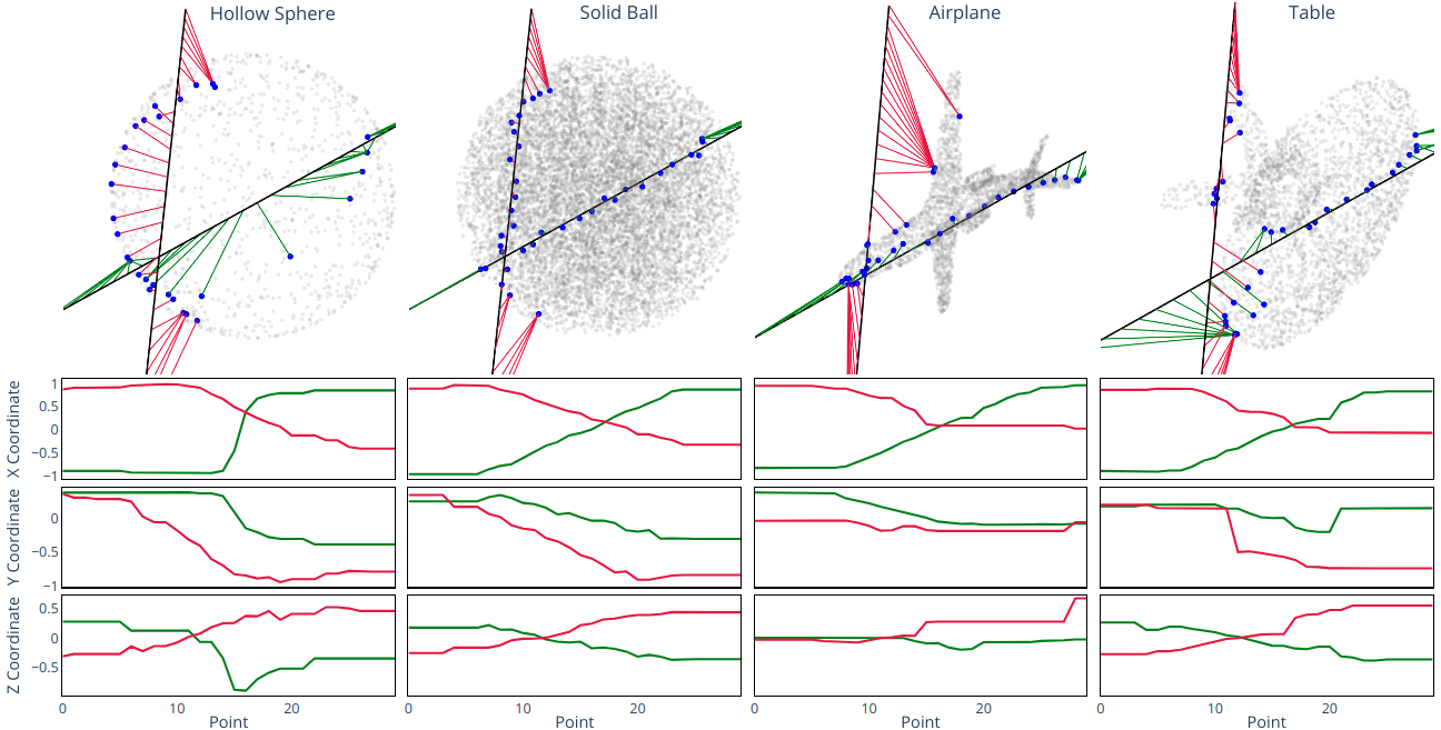
We propose a novel method for sampling, comparing, and analyzing point clouds, or other geometric objects, embedded in high-dimensional space. We call our approach “RaySense” because it “senses” the structure of the object $\Gamma$ by sending line segments through the ambient space occupied by $\Gamma$ and recording some functions of the nearest neighbors in $\Gamma$ to points on the line segment. Motivated by the X-ray transform, we will refer to the oriented line segments as “rays”. We can then work with this sampled data as a “sketch” of the original object $\Gamma$, which can be a point cloud, triangulated surface, volumetric representation, etc. A visualization of the proposed method applied to $3$D point clouds is provided in Fig. 1.

Figure 1: RaySense sketches using 30 sample points per ray. Row 1: visualization of two rays (black) through points sampled from various objects (gray). Closest point pairs are shown in green and red. Rows 2–4: the $x$, $\bm{y}$, and $z$ coordinates of the closest points to the ray.

Our method incorporates several ideas mentioned above:

• In the context of integral geometry, we also consider using affine subspaces to detect the underlying geometry. To overcome the discontinuity from the object representation relative to the topology of the ambient space (as is the case with point clouds), we search for nearest neighbors within the representation. To prevent the computational cost of high-dimensional operations in practice, we work with a low-dimensional affine subspace. In this paper, we use $1$-dimensional lines.

• In the context of inverse problems, our observed data consist of some points on $\Gamma$ obtained by the closest point projection of points on the rays. This is somewhat analogous to seismic imaging, where designated points on each ray correspond to geophones that record the first arrival time of waves from known sources.

• By using a fixed number of rays and sampling a fixed number of points along a ray, the resulting tensor from our method, the RaySense sketch, is of fixed size, even for point clouds with different cardinalities. Then, metrics suitable for comparing tensors are available for use, or one could consider other distance-based approaches to compare different RaySense sketches.

In this work we will focus exclusively on point clouds since it is one of the most challenging data representations for many algorithms. When the object is a point cloud, finding the RaySense samples is straightforward via discrete nearest neighbor searches. There are computationally efficient algorithms for performing nearest-in-Euclidean-distance neighbor searches. Examples include tree-based algorithms Bentley1975kdtree , grid-based algorithms tsai2002rapid , and building an indexing structure johnson2019billion . In very high dimensions, one may also consider randomized nearest neighbor search algorithms such as indyk1998approximate ; JonesOsipovRokhlin2011approxnn , or certain dimension reduction approaches.

The remaining paper is organized as follows: in Section 2, we provide a detailed description of the RaySense method; in Section 3, we present various properties of the RaySense method, along with theoretical analysis, including line integral approximations and salient point sampling; finally, in Section 4, we demonstrate that the concept of RaySense can be applied to many different downstream tasks, including salient point/outlier detection, point cloud registration, and point cloud classification.

1.1 Related work

In this section, we provide a more detailed discussion of the existing literature to contextualize our approach.

Integral geometry

In the field of Integral Geometry santalo2004integral , one uses the probability of intersection of affine subspaces of different dimensions with the target data manifold to deduce information about the manifold itself. For example, in the classic problem of Buffon’s needle, one determines the length of a dropped needle by investigating the probability of intersections with strips on a floor. Similarly, Crofton’s formula connects the length of a $2$D plane curve with the expected number of intersections with random lines. In these cases, the interaction information obtained from the “sensing” affine subspaces is binary: yes or no. One thus has a counting problem: how frequently affine subspaces intersect with the data manifold. From these probabilities, geometric information about the manifold can be extracted, relying on a duality between the dimensions of the “sensing” subspaces and the Hausdorff dimensions of the data set; see e.g., hadwiger1957vorlesungen ; klain1997introduction . Nevertheless, such approaches may be inefficient in practical computations.

Our idea of using rays is perhaps most-closely related to the X-ray transform, which coincides with the Radon Transform in 2D Natterer:computerized_tomography_siambook . In an X-ray transform, one integrates a given real-valued function defined in $\mathbb{R}^{d}$ along lines, while in the Radon transform, one integrates the given function restricted on hyperplanes of $\mathbb{R}^{d}$.

We advocate using lines (rays) to record information about the underlying data along each ray, instead of accumulating a scalar or binary “yes/no” information over each rays. In this paper, we collect points in the data set closest to the points on the rays, along with the values of some function at those points. With such data, we can compute approximate line integrals and relate our method to the X-ray transform.

Computer vision

From the perspective of the computer vision community, our method can be considered as a shape descriptor, mapping from 3D point sets to a more informative feature space where point sets can be easily compared. Generally, descriptors aim to capture statistics related to local and global features. See kazmi2013survey for a survey. More recently, researchers have combined shape descriptors with machine learning fang20153d ; rostami2019survey ; sinha2016deep ; xie2016deepshape . But all these works focus primarily for point sets in $3$D, RaySense applies more generally to data in arbitrary dimensions.

Some methods use machine learning directly on the point set to learn features for specific tasks, such as classification atzmon2018point ; klokov2017escape ; li2018pointcnn ; qi2017pointnet ; qi2017pointnet++ ; simonovsky2017dynamic ; wang2017cnn ; wang2019dynamic ; zhou2018voxelnet . PointNet qi2017pointnet pioneered deep learning on point clouds by applying independent operations on each point and aggregating features using a symmetric function. Building upon that, other architectures qi2017pointnet++ ; Shen_2018_CVPR exploit neighboring information to extract local descriptors. SO-Net li2018so uses self-organizing maps to hierarchically group nodes while applying fully-connected layers for feature extraction. PCNN atzmon2018point defines an extension and pulling operator similar to the closest point method ruuth2008simple ; macdonald2013simple to facilitate the implementation of regular convolution. DGCNN wang2019dynamic and PointCNN li2018pointcnn generalize the convolution operator to point sets.

In contrast, our approach uses the RaySense sketch as input rather than applying machine learning directly to the point set. In Sec. 4.5, we present a deep learning model for $3$D point cloud classification based on this idea. Our experiments suggest that the model is very efficient for classification, and the resulting classifiers can be robust against outliers by storing multiple nearest neighbors to points on the ray.

Unsupervised learning methods

Our method, by recording the closest points from the underlying point cloud, can be thought as a sampling scheme. However, the RaySense sampling is biased towards the “salient” points in the underlying geometry, as will be discussed in Sec. 3.2.1. By further retaining only the most frequently sampled points, RaySense resembles key-point detectors krig2016interest or compression algorithms. The idea of understanding the overall structure of the underlying data through key points is closely related to archetypal analysis cutler1994archetypal , which involves finding representative points (archetypes) in a dataset and using a convex combination of these archetypes to represent other points. See also Osting:ArchetypalAnalysis for a recent work on the consistency of archetypal analysis.

Incidentally, graham2017approximate also employs the concept of rays in conjunction with spherical volume to approximate the convex hull. Our method can also capture vertices of the convex hull when the rays are sufficiently long, as it will effectively sample points on the portions of the boundary that have relatively large positive curvature.

Farthest Point Sampling (FPS) is a widely-used sampling method in computational geometry and machine learning for selecting a subset of points from a larger dataset with the goal of maximizing their spread; see e.g. eldar1997farthest . The process begins by randomly picking a point from the dataset, followed by iterative selection of the point farthest from those already chosen, until a desired number of points are selected. This technique is useful for reducing the size of large datasets while preserving their overall structure. However, it can be computationally expensive and may not always yield the optimal solution. In two and three dimensions, assuming that the data distribution is supported in a bounded convex set with a smooth boundary, FPS tends to oversample areas with high curvature.

2 Methods

The essential elements of the proposed sampling strategy include (1) the data set $\Gamma\subset\mathbb{R}^{d}$; (2) the nearest neighbor (closest point) projection, $P_{\Gamma}$, to $\Gamma$; (3) a distribution of lines in $\mathbb{R}^{d}$.

The data set is given by a discrete set of $N$ points, each in $\mathbb{R}^{d}$:

$$\Gamma\subset\mathbb{R}^{d},\qquad\Gamma=\{\bm{X}_{i}\}_{i=1}^{N},\qquad\bm{X}_{i}\in\mathbb{R}^{d},$$ (1)

(later for certain results we will place more assumptions, for example that $\Gamma$ might be sampled from a density.)

Let $\mathcal{L}$ denote a distribution of lines, parameterized by $\bm{\theta}\in\mathbb{S}^{d-1}$ and $\bm{b}\in\mathbb{R}^{d}$, let $\bm{r}(s)$ denote a line in $\mathcal{L}$ parameterized by its length

$$\bm{r}(s)=\bm{b}+s\bm{\theta}.$$

The parameterization gives an orientation to the line, and thereby we refer to $\bm{r}$ as a ray. Along $\bm{r}(s)$, we sample from the data set $\Gamma$ using the nearest neighbor projection

$$\mathcal{P}_{\Gamma}\bm{r}(s)\in\operatorname*{arg\,min}_{\bm{y}\in\Gamma}\|\bm{r}(s)-\bm{y}\|_{2}.$$ (2)

In cases of non-uniqueness, we choose arbitrarily.

Using the nearest neighbors, we define various RaySense sampling operators denoted with $\mathcal{S}$ which sample from the point cloud $\Gamma$ into some “feature space” $\mathbb{X}\subset\mathbb{R}^{c}$. The simplest choice is the feature space of closest points defined next.

Definition 1.

The closest point feature space is sampled by

$$\mathcal{S}[\Gamma]:\mathbb{R}^{d}\to\mathbb{R}^{d},\qquad\mathcal{S}[\Gamma](\bm{r}(s))=\mathcal{P}_{\Gamma}\bm{r}(s),\qquad\bm{r}\sim\mathcal{L}.$$ (3)

One might also be interested in the value of a scalar or vector function (e.g., color or temperature data at each point in the point cloud).

Definition 2.

The RaySense sampling operator of a function $g:\Gamma\to\mathbb{R}^{c}$ is

$$\mathcal{S}[\Gamma,g]:\mathbb{R}^{d}\to\mathbb{R}^{c},\qquad\mathcal{S}[\Gamma,g](\bm{r}(s))=g\big{(}\mathcal{P}_{\Gamma}\bm{r}(s)\big{)},\qquad\bm{r}\sim\mathcal{L}.$$ (4)

Note for the identity function we have $\mathcal{S}[\Gamma,\mathrm{id}]=\mathcal{S}[\Gamma]$.

We will further present examples involving the use of multiple nearest neighbors, where the $\eta$-th nearest neighbor is

$$\mathcal{P}_{\Gamma}^{\eta}(\bm{r}(s)) :=\operatorname*{arg\,min}_{\bm{y}\in\Gamma\setminus\{\mathcal{P}_{\Gamma}^{1}\bm{r}(s),\ldots,\mathcal{P}_{\Gamma}^{\eta-1}\bm{r}(s)\}}\|\bm{r}(s)-\bm{y}\|_{2},$$ (5)

with $\mathcal{P}_{\Gamma}^{1}:=\mathcal{P}_{\Gamma}$. We can then capture the $\eta$-th nearest neighbor in our sampling.

Definition 3.

The RaySense sampling operator of the $\eta$-th nearest neighbor is denoted by:

$$\mathcal{S}[\Gamma,\eta]:\mathbb{R}^{d}\times\mathbb{N}\to\mathbb{R}^{d},\qquad\mathcal{S}[\Gamma,\eta](\bm{r}(s))=\mathcal{P}^{\eta}_{\Gamma}\bm{r}(s),\qquad\bm{r}\sim\mathcal{L}.$$ (6)

The distance and direction from $\bm{r}(s)$ to $\mathcal{P}_{\Gamma}\bm{r}(s)$ is sometimes useful: we sample that information using the vector from $\bm{r}(s)$ to $\mathcal{P}_{\Gamma}\bm{r}(s)$:

Definition 4.

The RaySense sampling operator of the vector between a point on the ray and the nearest neighbor in $\Gamma$ is

$$\mathcal{S}[\Gamma,\hat{1}]:\mathbb{R}^{d}\times\mathbb{N}\to\mathbb{R}^{d},\qquad\mathcal{S}[\Gamma,\hat{1}](\bm{r}(s))=\mathcal{P}_{\Gamma}\bm{r}(s)-\bm{r}(s),\qquad\bm{r}\sim\mathcal{L},$$ (7a)

and more generally

$$\mathcal{S}[\Gamma,\hat{\eta}]:\mathbb{R}^{d}\times\mathbb{N}\to\mathbb{R}^{d},\qquad\mathcal{S}[\Gamma,\hat{\eta}](\bm{r}(s))=\mathcal{P}^{\eta}_{\Gamma}\bm{r}(s)-\bm{r}(s),\qquad\bm{r}\sim\mathcal{L}.$$ (7b)

We can augment the feature space by combining these various operators, concatenating the output into a vector $\mathcal{X}\in\mathbb{R}^{c}$. We indicate this “stacking” with a list notation in $\mathcal{S}$, for example the first three closest points could be denoted:

$$\mathcal{S}\big{[}\Gamma,[1,2,3]\big{]}(\bm{r}(s))=\begin{bmatrix}\mathcal{P}^{1}_{\Gamma}\bm{r}(s)\\ \mathcal{P}^{2}_{\Gamma}\bm{r}(s)\\ \mathcal{P}^{3}_{\Gamma}\bm{r}(s)\end{bmatrix}\!,\quad\bm{r}\sim\mathcal{L},$$ (8)

or the closest point, its vector from the ray, and the value of a function $g$ could all be denoted:

$$\mathcal{S}\big{[}\Gamma,[1,\hat{1},g]\big{]}(\bm{r}(s))=\begin{bmatrix}\mathcal{P}_{\Gamma}\bm{r}(s)\\ \mathcal{P}_{\Gamma}\bm{r}(s)-\bm{r}(s)\\ g\big{(}\mathcal{P}_{\Gamma}\bm{r}(s)\big{)}\end{bmatrix}\!,\quad\bm{r}\sim\mathcal{L}.$$ (9)

These stacked feature spaces are used in the line integral approximation Sec. 3.1.3 and in our neural network Sec. 4.5.

In summary, a RaySense sketch $\mathcal{S}[\Gamma,\ldots]$ depends on nearest neighbors in the data set $\Gamma$, and operates on a ray from the distribution $\mathcal{L}$. It maps a ray $\bm{r}(\cdot)$ to a piecewise curve in the chosen feature space $\mathbb{X}$.

2.1 Discretization

We propose to work with a discretized version of the operator, which we shall call a RaySense sketch tensor. First, we take $m$ i.i.d. samples from the distribution $\mathcal{L}$ and define $m$ rays correspondingly. We consider $n_{r}$ uniformly-spaced points along each ray, with corresponding spacing $\delta r$. We then work with a finite segment of each line (for example, $0\leq s\leq 1$). Appendix A shows some different distributions of lines, and details for choosing segments from them. With $\bm{r}_{i,j}$ denoting the $j$-th point on the $i$-th ray, we define the discrete RaySense sketch of $\Gamma$ in the closest point feature space as

$$\mathcal{S}_{m,\delta r}[\Gamma\mathchar 24635\relax\;\mathcal{L}]_{i,j}:=\mathcal{P}_{\Gamma}\bm{r}_{i,j},$$ (10a)

or the discrete RaySense sketch of a function $$g$$:

$$\mathcal{S}_{m,\delta r}[\Gamma,g\mathchar 24635\relax\;\mathcal{L}]_{i,j}:=g\big{(}\mathcal{P}_{\Gamma}\bm{r}_{i,j}\big{)},$$ (10b)

(and similarly for the various more-general feature spaces mentioned earlier).

Thus, $\mathcal{S}_{m,\delta r}$ is an array with $m$ entries, where each entry is an array of $n_{r}$ vectors in $R^{c}$; an $m\times n_{r}\times c$ tensor. We will also denote these tensors as “$\mathcal{S}(\Gamma)$” and “$\mathcal{S}(\Gamma,g)$” when $m$ and $\delta r$ are not the focus of the discussion. In any case, we regard $\mathcal{S}(\Gamma)$ as a “sketch” of the point cloud $\Gamma$ in a chosen feature space $\mathbb{X}$.

2.2 Operations on RaySense sketches

In this paper, we will analyze the outcomes of the following operations performed on the RaySense sketches. After discretization, each operation can be expressed as one or more summations performed on the sketches.

2.2.1 Histograms

One simple operation is to aggregate the sampled values for the feature space and count their corresponding sampling frequencies, which results in a histogram demonstrating the discrete distribution of the corresponding features. For example, when considering the closest point feature space $\mathcal{S}[\Gamma]$, the value of a bin in the histogram, denoted by $H_{k}$, represents the number of times $\bm{x}_{k}\in\Gamma$ being sampled by RaySense:

$$H_{k}:=H\big{(}\bm{x}_{k}\mathchar 24635\relax\;\mathcal{S}_{m,\delta r}[\Gamma]\big{)}=\sum_{i=1}^{m}\sum_{j=1}^{n_{r}}\chi_{\bm{x}_{k}}\big{(}{\mathcal{S}[\Gamma]_{i,j}}\big{)},$$ (11)

where $\chi_{\bm{x}_{k}}$ denotes the indicator function for the coordinates of $\bm{x}_{k}$. The histograms discard locality information in the sketch, treating it essentially as a weighted subsampling of $\Gamma$, as the aggregation process involves combining the values without considering the specific rays from which they originated. Sec. 3.2.2 further discusses properties of the histogram.

2.2.2 Line integrals

In many applications, it is useful to maintain some “locality”. One such operation is the line integral along each ray $\int_{0}^{1}g(\bm{r}(s))\,\textrm{d}s$. However, for point cloud data, exact information of $g$ along the ray $\bm{r}(s)$ is not accessible, we instead consider the integral along the associated path in feature space, $\int_{0}^{1}\mathcal{S}[\Gamma,g]\left(\bm{r}(s)\right)\,\textrm{d}s$, which we call a RaySense integral. We investigate the relationship between the two in Sec. 3.1.3.

In the discrete setting, we can use a simple Riemann sum quadrature scheme to approximate the RaySense integral along the $i$-th ray:

$$\int_{0}^{1}\mathcal{S}[\Gamma,g]\left(\bm{r}_{i}(s)\right)\,\textrm{d}s\approx\sum_{j=1}^{n_{r}}\mathcal{S}[\Gamma,g]_{i,j}\,\delta r.$$ (12a)

Or in most of our examples, we approximate using the Trapezoidal Rule:

$$\int_{0}^{1}\mathcal{S}[\Gamma,g]\left(\bm{r}_{i}(s)\right)\,\textrm{d}s\approx\sum_{j=1}^{n_{r}}w_{j}\,\mathcal{S}[\Gamma,g]_{i,j}\,\delta r,\quad\text{with weights $w=\left\langle\tfrac{1}{2},1,\ldots,1,\tfrac{1}{2}\right\rangle$,}$$ (12b)

and thus quadrature errors, typically $$\mathcal{O}(\delta r^{2})$$, are incurred TrefethenWeideman:trapezoidalrule . Unpacking the notation, we can rewrite this as

$$\sum_{j=1}^{n_{r}}w_{j}g(\mathcal{P}_{\Gamma}\bm{r}_{i}(s_{j}))\,\delta r.$$ (12c)

2.2.3 Convolutions

Similar to line integrals, we will compute convolutions along the rays

$$\big{(}K*\mathcal{S}[\Gamma,\ldots](\bm{r})\big{)}(t)=\int_{-\infty}^{\infty}K(s)\mathcal{S}[\Gamma,\ldots](\bm{r}(t-s))\,\textrm{d}s,$$

where $K$ is some compactly-supported kernel function and $\mathcal{S}[\Gamma,\ldots]$ is one of the RaySense sampling operators. In the discrete setting, this can be written as weighted sums of $\mathcal{S}[\Gamma,\ldots]$, or as band-limited matrix multiplication. In Sec. 4.5, the discrete weights associated with discrete convolutions are the parameters of a neural network model.

Note unlike the previous cases, for non-symmetric kernels the orientation of the rays matters.

2.3 Comparing data sets

Since the sketch for any point set is a fixed-size tensor storing useful feature information, one might compare two point sets (of potentially different cardinalities) via comparing the RaySense sketches.

A natural idea is to choose a suitable metric to define the distances between the RaySense sketch tensors.

The Frobenius norm of the sketch tensor is suitable if the sketches contain the distance and the closest point coordinates. For data sampled from smooth objects, such information along each ray is piecewise continuous. Thus, if the sketches are generated using the same set of sampling rays, one may compare the RaySense sketches of different data sets using the Frobenius norm.

Wasserstein distances are more appropriate for comparison of histograms of the RaySense data, especially when the sketches are generated by different sets of random rays. The normalized histograms can be regarded as probability distributions. In particular, notice (Fig. 6) that RaySense histograms tend to have “spikes” that correspond to the salient points in the data set; $\ell^{2}$ distances are not adequate for comparing distributions with such features.

Here we briefly describe the Wasserstein-1 distance, or Earth mover’s distance, that we used in this paper. Let $(X,\mu_{1})$ and $(\tilde{X},\mu_{2})$ be two probability spaces and $F$ and $G$ be the cumulative distribution functions of $\mu_{1}$ and $\mu_{2}$, respectively. The Wasserstein-1 distance is defined as

$$W_{1}(\mu_{1},\mu_{2}):=\int_{\mathbb{R}}\lvert F(t)-G(t)\rvert\,\mathrm{d}t.$$

Neural networks:   One can consider using a properly designed and trained neural network. In Sec. 4.5, we present a neural network model, RayNN, for comparing point clouds in three dimensions based on RaySense sketches.

3 Properties of RaySense

In this section, we introduce several notable properties associated with our proposed method. Specifically, we begin by analyzing the characteristics of the method when utilizing a single ray, i.e., $m=1$. We subsequently proceed to discuss how the RaySense sketch, resulting from using multiple rays, effectively utilizes and inherits the identified traits. Through these analyses, we aim to provide a more rigorous and comprehensive understanding of the properties and potential applications of our proposed method.

Assumptions and notations for this section:

• The point set $\Gamma$, is a realization of a collection of $N$ i.i.d. random vectors $\{\bm{X}_{i}\}_{i=1}^{N}$, with each $\bm{X}_{i}\in\mathbb{R}^{d}$.

• The probability space induced by the random vector $\bm{X}_{i}$ is $(\mathbb{R}^{d},\mathcal{F},\mu)$, where $\mathcal{F}$ is the Borel $\sigma$-algebra on $\mathbb{R}^{d}$ and $\mu$ is a probability measure.

• The induced probability measure $\mu$ is also known as the distribution of $\bm{X}_{i}$, with compactly supported Lipschitz density $\rho$.

• The RaySense sketch uses the closest points feature space (3).

• In the case that $\bm{r}(s)$, for some $s$, has more than one nearest neighbor, we will randomly assign one.

• A ray, denoted by $\bm{r}(s)$, $0\leq s\leq 1$, generated by the method introduced in Sec. A, is given in the embedding space $\mathbb{R}^{d}$ of $\Gamma$, and the support of $\rho$ is centered.

• We assume $\textrm{supp}(\rho)$ can be covered by a finite union of hypercubes $\{\Omega_{j}\}_{j}$ in $\mathbb{R}^{d}$, each of non-zero probability measure, i.e., $\textrm{supp}(\rho)\subset\bigcup_{j}\Omega_{j}$, with $P_{\Omega_{j}}=\int_{\bm{x}\in\Omega_{j}}\rho(\bm{x})\mathrm{d}\bm{x}>0$, and $\{\Omega_{j}\}_{j}$ overlap with each other only on sets of measure zero.

Note that by A2-A3, we may regard $\rho$ as representing the density of a solid body in $\mathbb{R}^{d}$. In other words, $\Gamma$ does not consist of samples from a lower dimensional set. (RaySense can sample much more general sets, but the line integral analysis (Sec. 3.1.3) and the argument of sampling convex hull (Sec. 3.2.1) of this section may not hold.)

Much of our analysis is based on the Voronoi cells associated with each point in the point cloud.

Definition 5.

The Voronoi cell of $\bm{x}\in\Gamma$ is defined as

$$V(\bm{x}):=\{\bm{y}\in\mathbb{R}^{d}:\mathcal{P}_{\Gamma}\bm{y}=\bm{x}\}.$$ (13)

In practice, we often sample rays $\bm{r}\sim\mathcal{L}$ of finite length as in Fig. 2, i.e. $\{\bm{r}_{i}\}_{i=1}^{m}\subset B_{R}(0)$ for some $R$. Correspondingly, we define the truncated Voronoi cell:

$$V^{R}(\bm{x}):=\{\bm{y}\in B_{R}(0):\mathcal{P}_{\Gamma}\bm{y}=\bm{x}\}.$$ (14)

3.1 Properties of sampling with a single ray

3.1.1 Sampling points with larger Voronoi cells

For discrete point sets, the likelihood that a ray senses a particular point is closely linked to the size of the Voronoi cell of the point. This relationship arises from the practice of utilizing closest point sampling, which governs the selection of points by a given ray. In this regard, the Voronoi cell of a point in the point clouds is a fundamental geometric construct that plays a key role in determining the probability of detection. This observation is visually depicted in Fig. 2, which demonstrates that points having larger Voronoi cells are more likely to be detected by a given ray.

Figure 2: A simple 2D point set (gray). Two rays (black) sense nearest neighbors of the point set (blue). Singular points, such as the tip of the tail, have larger Voronoi cells (dashed lines) and are more likely to be sampled. Closest point pairings are shown in green and red.

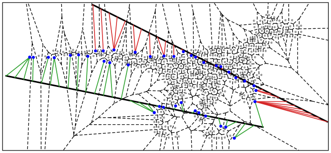
We refer to points with relatively large Voronoi cells as the “salient points” of $\Gamma$. When the probability density for $\Gamma$ is compactly supported, the salient points of $\Gamma$ tend to be situated in close proximity to geometric singularities present on the boundary of the support of the density; see Fig. 2 for a demonstration. This saliency characteristic will be further elaborated on in Sec. 3.2.1, where we will demonstrate how it manifests as the biased subsampling property of the RaySense method.

Furthermore, connections between the probability of a point $\in\Gamma$ being sampled and the size of its Voronoi cell can be made explicit in the following derivation. Let $B_{R}(0)\in\mathbb{R}^{d}$ be a solid dimension-$d$ ball of radius $R$ containing all the rays, and $\Gamma\subsetneq B_{R}(0)$ the finite point set containing $N$ distinct points. Let $V_{k}:=V(\bm{x}_{k})$ denote the Voronoi cell for the $k$-th point, $\bm{x}_{k}$ in $\Gamma$ as in Def. 5. Let $\ell_{k}(\bm{r})$ denote the length of the segment of a ray, $\bm{r}$, that lies in the truncated Voronoi cell $V^{R}_{k}$. If $\bm{r}$ does not intersect $V_{k}$, $\ell_{k}(\bm{r}):=0$. Thus, $\ell_{k}(\bm{r})$ is a random variable indicating how much a ray $\bm{r}$ senses $\bm{x}_{k}\in\Gamma$ , and we denote its expectation by $\mathbb{E}[\ell_{k}]$; in other words,

$$\mathbb{E}[\ell_{k}]:=\int\ell_{k}(\omega)\,\mathrm{d}\mu_{\mathcal{L}}(\omega)=\mathbb{E}_{\bm{r}\sim\mathcal{L}}\Big{[}\int_{r}\chi_{V_{k}}\big{(}\bm{r}(s)\big{)}\mathrm{d}s\Big{]},$$ (15)

where $\mu_{\mathcal{L}}$ is the probability measure corresponding to the distribution of lines $\mathcal{L}$ introduced in Sec. 2, and $\chi_{V_{k}}$ is the indicator function of the Voronoi cell $V_{k}$. Consequently, the frequency of a ray $\bm{r}$ sampling a point $\bm{x}_{k}\in\Gamma$ is proportional to the $d$-dimensional Lebesgue measure of its Voronoi cell $V_{k}=V(\bm{x}_{k})$.

3.1.2 Sampling consistency

The Voronoi cell perspective provides a framework to analyze certain properties of RaySense. We will show in Theorem 4 that the sampling from a specific ray is consistent when the number of points $N$ in the point clouds is large enough. We begin with some lemmas, with proofs appearing in Appendix C.

Our first lemma tells us how large $N$ must be in order to have at least one sample in any region achieving a certain probability measure.

Lemma 1.

Suppose that $\textrm{supp}(\rho)$ satisfies assumption A$7$. Let $\Gamma$ be a set of $N$ i.i.d. random samples drawn from $\mu$, and $p_{0}\in(0,1)$. If the number of sample points $N>\nu\big{(}P\big{)}$ where $\nu:(0,1]\mapsto\mathbb{R}^{+}$ is defined by

$$\nu\big{(}P\big{)}:=\frac{\sqrt{\ln{(\frac{2}{1-p_{0}})}\big{(}\ln{(\frac{2}{1-p_{0}})}+2P\big{)}}+P+\ln{(\frac{2}{1-p_{0}})}}{P^{2}},$$ (16)

then, with probability greater than $p_{0}$, at least one of the samples lies in every $\Omega_{j}$ with $P_{\Omega_{j}}\geq P$. Additionally, we note bounds for $\nu(P)$:

$$\frac{2\ln{(\frac{2}{1-p_{0}})}+P}{P^{2}}<\nu\big{(}P\big{)}<\frac{2\ln{(\frac{2}{1-p_{0}})}+3P}{P^{2}}.$$ (17)

We notice that for any fixed $p_{0}>0$, $\nu\left(P\right)\sim\mathcal{O}\left(1/P^{2}\right)$ as $P\to 0$ indicating $\nu\left(P\right)$ is inversely proportional to $P^{2}$ asymptotically. This matches with the intuition that more points are needed to ensure sampling in regions with smaller probability measure.

The next two lemmas reveal that the volume of the Voronoi cell for a sample point amongst the others in the point cloud $\Gamma$ decreases to zero with high probability as the number of sampled points tends to $\infty$.

Lemma 2.

Suppose $\rho$ is $L$-Lipschitz and $\textrm{supp}(\rho)$ satisfies assumption A7. Given $\Gamma$ a set of $N$ i.i.d. random samples drawn from $\mu$, for $N$ large enough, the size of the Voronoi cell of a sample point $\bm{x}\in\Gamma$ in the interior of $\textrm{supp}(\rho)$ is inversely proportional to its local density $\rho(\bm{x})$, and with probability at least $p_{0}$ its diameter has the following upper bound:

$$\textrm{diam}(V(\bm{x}))\leq 3\sqrt{d}\left(\frac{21+7\big{(}9+8N\ln{(\frac{2}{1-p_{0}})}\big{)}^{1/2}}{6\rho(\bm{x})N}\right)^{\!\!\frac{1}{d}}\!\!.$$

When the underlying distribution $\mu$ is uniform, $\rho(\bm{x})$ is the same everywhere inside $\textrm{supp}(\rho)$, therefore the Voronoi diameter for every $\bm{x}$ in the interior should shrink uniformly. However, a better bound can be obtained for this case, shown in the following lemma.

Lemma 3.

If $\mu$ is a uniform distribution, then given $\Gamma$ with $N$ large enough, with probability at least $p_{0}$, the diameter of the Voronoi cell of any sample point in the interior has the bound

$$\textrm{diam}(V)\leq 3\sqrt{d}\left(\left\lfloor\frac{1}{c(N)N}\ln{\frac{N}{1-p_{0}}}\right\rfloor\right)^{\!\frac{1}{d}}\!\!,$$

with some $c(N)$ such that $c(N)\to 1$ as $N\to\infty$.

Theorem 4 (Consistency of sampling).

Under A$1$-A$7$, suppose $\Gamma_{1}$ and $\Gamma_{2}$ are two point clouds sampled from the same distribution, with $N_{1}$ and $N_{2}$ points respectively, where in general $N_{1}\neq N_{2}$. Assume further that $\textrm{supp}(\rho)$ is convex. For a ray $\bm{r}(s)$ using $n_{r}$ uniformly-spaced discrete points to sample, for $N=\min(N_{1},N_{2})$ sufficiently large, the RaySense sketches in the closest point feature space $S[\Gamma_{1}]$ and $S[\Gamma_{2}]$ satisfy

$$\Big{\lVert}S[\Gamma_{1}]-S[\Gamma_{2}]\Big{\rVert}_{F}\leq\varepsilon\big{(}N\big{)},$$ (18)

where $\varepsilon>0$ and $\varepsilon\to 0$ as $N\to\infty$.

Remark 1.

The assumption that $\textrm{supp}(\rho)$ is convex is stronger than needed in many cases; it excludes the situation where some point $\bm{r}_{i,j}$ in the discretized ray set is equidistant to two or more points on the non-convex $\textrm{supp}(\rho)$ that are widely separated, which could lead to an unstable assignment of nearest neighbors. However, in practical scenarios where a ray is chosen randomly, this situation is unlikely to occur. Further details can be found at the end of Appendix C.

The consistency of sampling ensures the RaySense data on a specific ray would be close when sampling the same object, therefore one can expect a similar property for the RaySense sketch tensor where multiple rays are used, which will be discussed in Sec. 3.2.1.

3.1.3 Approximate line integrals

We demonstrate that the RaySense approach enables the computation of line integrals of functions defined on the points in a point cloud. Suppose we have a point cloud $\Gamma$ representing an object in $\mathbb{R}^{d}$. As $N$ increases, the point cloud becomes denser, and for any $\bm{r}(s)$ lies inside $\textrm{supp}(\rho)$, $\mathcal{P}_{\Gamma}\bm{r}(s)\approx\bm{r}(s)$ as the Voronoi cells shrink around each point in $\Gamma$. If we have a smooth function $g:\mathbb{R}^{d}\mapsto\mathbb{R}$ evaluated on the point cloud, then $g(\mathcal{P}_{\Gamma}\bm{r}(s))\approx g(\bm{r}(s))$ and we expect that integrals of $g$ along lines can be approximated by integrals of the RaySense sketch $\mathcal{S}[\Gamma,g]$ introduced in Sec. 2.2.2 (and quadrature of the discrete RaySense sketch $\mathcal{S}_{m,\delta r}[\Gamma,g]$).

The following shows that the RaySense integral is an approximation to the line integral along $\bm{r}(s)$ provided the point cloud is dense enough.

Theorem 5.

Suppose that $g\in C(\mathbb{R}^{d}\mathchar 24635\relax\;\mathbb{R})$ is $J$-Lipschitz, ray $\bm{r}(s)\in\textrm{supp}(\rho)$ for $0\leq s\leq 1$, and $\Gamma$ is a set of $N$ i.i.d. random samples drawn from $\mu$, with corresponding RaySense sketch $\mathcal{S}[\Gamma,g]$, then the difference between the RaySense integral of $g$ and the line integral of $g$ has the following bound:

$$\Big{\lvert}\int_{0}^{1}g\big{(}\bm{r}(s)\big{)}\mathrm{d}s-\int_{0}^{1}g\big{(}\mathcal{P}_{\Gamma}\bm{r}(s)\big{)}\mathrm{d}s\Big{\rvert}\leq J\sum_{\bm{x}\in\Gamma}\int_{0}^{1}\chi_{V(\bm{x})}\big{(}\bm{r}(s)\big{)}\lVert\bm{r}(s)-\mathcal{P}_{\Gamma}\bm{r}(s)\rVert\mathrm{d}s,$$ (19)

where $\chi_{V(\bm{x})}$ is the indicator function of the Voronoi cell $V(\bm{x})$ for $\bm{x}\in\Gamma$.

Proof: For a fixed number of sampling points $N$, the approximation error is given by

$$\Big{\lvert}\int_{0}^{1}g\big{(}\bm{r}(s)\big{)}\mathrm{d}s-\int_{0}^{1}g\big{(}\mathcal{P}_{\Gamma}\bm{r}(s)\big{)}\mathrm{d}s\Big{\rvert} \leq\int_{0}^{1}\Big{\lvert}g\big{(}\bm{r}(s)\big{)}-g\big{(}\mathcal{P}_{\Gamma}\bm{r}(s)\big{)}\Big{\rvert}\mathrm{d}s$$

$$=\sum_{\bm{x}\in\Gamma}\int_{0}^{1}\chi_{V(\bm{x})}\big{(}\bm{r}(s)\big{)}\Big{\lvert}g\big{(}\bm{r}(s)\big{)}-g\big{(}\mathcal{P}_{\Gamma}\bm{r}(s)\big{)}\Big{\rvert}\mathrm{d}s$$

$$\leq J\sum_{\bm{x}\in\Gamma}\int_{0}^{1}\chi_{V(\bm{x})}\big{(}\bm{r}(s)\big{)}\lVert\bm{r}(s)-\mathcal{P}_{\Gamma}\bm{r}(s)\rVert\mathrm{d}s.$$

In scattered data interpolation, the nearest neighbor interpolation would have an error of $\mathcal{O}(h)$ where $h=\max_{k}\textrm{diam}(V_{k})$. Integration of the interpolated data would result in an error of $\mathcal{O}(h^{2})$, consistent with Theorem 5.

Intuitively, we expect the RaySense line integral to converge in the limit of $N\to\infty$. Here we show the corresponding convergence result for the case of uniform density from the perspective of a Poisson point process daley2003introduction . Details of the proof are given in Appendix D.

Theorem 6.

Suppose $g\in C(\mathbb{R}^{d}\mathchar 24635\relax\;\mathbb{R})$ is $J$-Lipschitz, $\rho$ is uniform and satisfies assumption A$7$, and the ray $\bm{r}(s)\in\textrm{supp}(\rho)$ for $0\leq s\leq 1$, then given $\Gamma$ a set of $N$ i.i.d. random samples as a realization of a Poisson point process with the corresponding RaySense sketch $\mathcal{S}[\Gamma,g]$ for the ray, the probability that the following holds tends to 1 as $N\rightarrow\infty:$

$$\Big{\lvert}\int_{0}^{1}g\big{(}\bm{r}(s)\big{)}\mathrm{d}s-\int_{0}^{1}g\big{(}\mathcal{P}_{\Gamma}\bm{r}(s)\big{)}\mathrm{d}s\Big{\rvert}\leq c(d,J)N^{-\frac{1}{d}+\varepsilon(d+1)}\!\!,$$

for any small $\varepsilon>0$.
When $\varepsilon<\frac{1}{(d+1)^{2}}$, the line integral error converges to $0$ as $N\to\infty$ in a rate $\mathcal{O}(N^{-\frac{1}{d}})$.

We first confirm this rate with numerical experiments. We return to explore applications of integral transforms in Sec. 4.3. Fig. 3 shows convergence studies of the RaySense integrals for the uniform density case from Theorem 6. The 5-d example uses an integrand of $g(x_{1},x_{2},x_{3},x_{4},x_{5})=\cos(x_{1}x_{2})-x_{4}x_{5}\sin(x_{3})$ and a line $\bm{r}(s)=\frac{\bm{v}}{\|\bm{v}\|}s+\frac{\left\langle 1,1,1,1,1\right\rangle}{10}$ with $\bm{v}=\left\langle 2,3,4,5,6\right\rangle$. In 4-d, 3-d and 2-d, we use $g(x_{1},x_{2},x_{3},x_{4},1)$, $g(x,y,z,1,1)$ and $g(x,y,0,0,0)$ respectively, and drop unneeded components from the line. The exact line integrals were computed with the Octave Symbolic package OctaveSymbolicPkg which uses SymPy sympy and mpmath mpmath . Each experiment is averaged over 50 runs.

Figure 3: Convergence studies for line integrals approximating from the RaySense sketch on point clouds sampled from a uniform density, in dimensions $d=2,3,4,5$. Horizontal dashed lines indicate error inherent to the trapezoidal rule quadrature schemes. Diagonal dashed lines indicate different convergence rates.

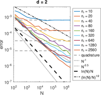
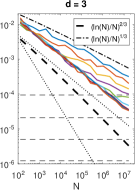
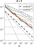
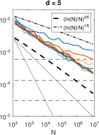
In Fig. 3, we see that for each fixed number of sample points $n_{r}$ along the ray, the error decreases at the rate discussed above. From the factor of two in the distance between the results of each fixed $n_{r}$, infer a first-order decrease in $n_{r}$, and taken together an overall faster rate of convergence if both $N$ and $n_{r}$ are increased. In all cases in Fig. 3, the experimental convergence rate is bounded by $\mathcal{O}\left(\frac{1}{N}\ln N\right)^{1/d}$ which is asymptotically close to the predicted rate given in Theorem 6 since $\varepsilon$ can be taken arbitrarily small. However, when $n_{r}$ is large, we appear to achieve a faster rate of $\mathcal{O}\left(\frac{1}{N}\ln N\right)^{2/d}$. This suggests a tighter analysis may be possible in the future.

3.1.4 Ray not fully contained in $\textrm{supp}(\rho)$

For any portion of $\bm{r}(s)$ that lie outside of $\textrm{supp}(\rho)$ such portion should take no values when computing the line integral if $g$ is only defined on $\textrm{supp}(\rho)$. Thus, the post-processing procedure involves eliminating sampling points on $\bm{r}(s)$ that are outside of $\textrm{supp}(\rho)$. When $N$ is large, this can be accomplished by augmenting the RaySense feature space with vectors to the closest point as in (9) rather than using A4, and redefining $g(\mathcal{P}_{\Gamma}\bm{r}(s))=0$ if the distance to the closest point of $\bm{r}(s)$ is beyond some small threshold.

3.2 Properties of sampling with multiple rays

When applying RaySense to the point set $\Gamma\in\mathbb{R}^{d}$ with $m$ rays and $n_{r}$ points on each ray, the RaySense sketch $S(\Gamma)$ is an $m\times n_{r}\times d$ tensor defined in (10a). In the following sections, we investigate properties of the RaySense sketch as an extension of the properties of RaySense using a single ray previously discussed.

3.2.1 Biased samplings toward salient points

A direct consequence from Sec. 3.1.1 is that the RaySense sketch $S(\Gamma)$ tends to repeatedly sample points with larger Voronoi cells, indicating a bias toward these salient points. Fig. 4 demonstrates this property by visually presenting the frequency of the sampled points by the size of the plotted blue dots.

Figure 4: Points sampled by RaySense using different number of rays are indicated as blue dots. The larger blue dots correspond to points that are more frequently sampled. The effect of sampling saliency becomes more apparent as the number of rays increases. Each ray contains 30 sample points.

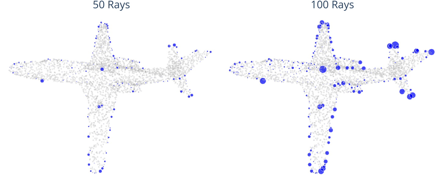
Another notable feature from Fig. 4 is that the biased subsample generated by RaySense also depicts the outline of the object. This is because points with larger Voronoi cells usually situate near the boundary and regions with positive curvatures. The following proposition gives a sufficient condition to identify such points:

Proposition 7.

Vertices of the convex hull of the point cloud $\Gamma$ will be frequently sampled by RaySense, when using sufficiently long rays.

Proof: Because $\textrm{supp}(\rho)$ is compact, the Voronoi cell for vertices on the convex hull are unbounded. Therefore, one can make the volumes of their truncated Voronoi cell (14), as large as desired by using rays with suitable length. And recall from Sec. 3.1.1 that the frequency of being sampled is closely related to the measures of the Voronoi cell.

Remark 2.

The arguments in the proof also implies when the length of the line segment $\to\infty$, with high probability RaySense is sampling mostly the convex hull of the point sets when $\textrm{supp}(\rho)$ is compact. This can be viewed as a different approach to approximate convex hulls using rays and curvatures from graham2017approximate .

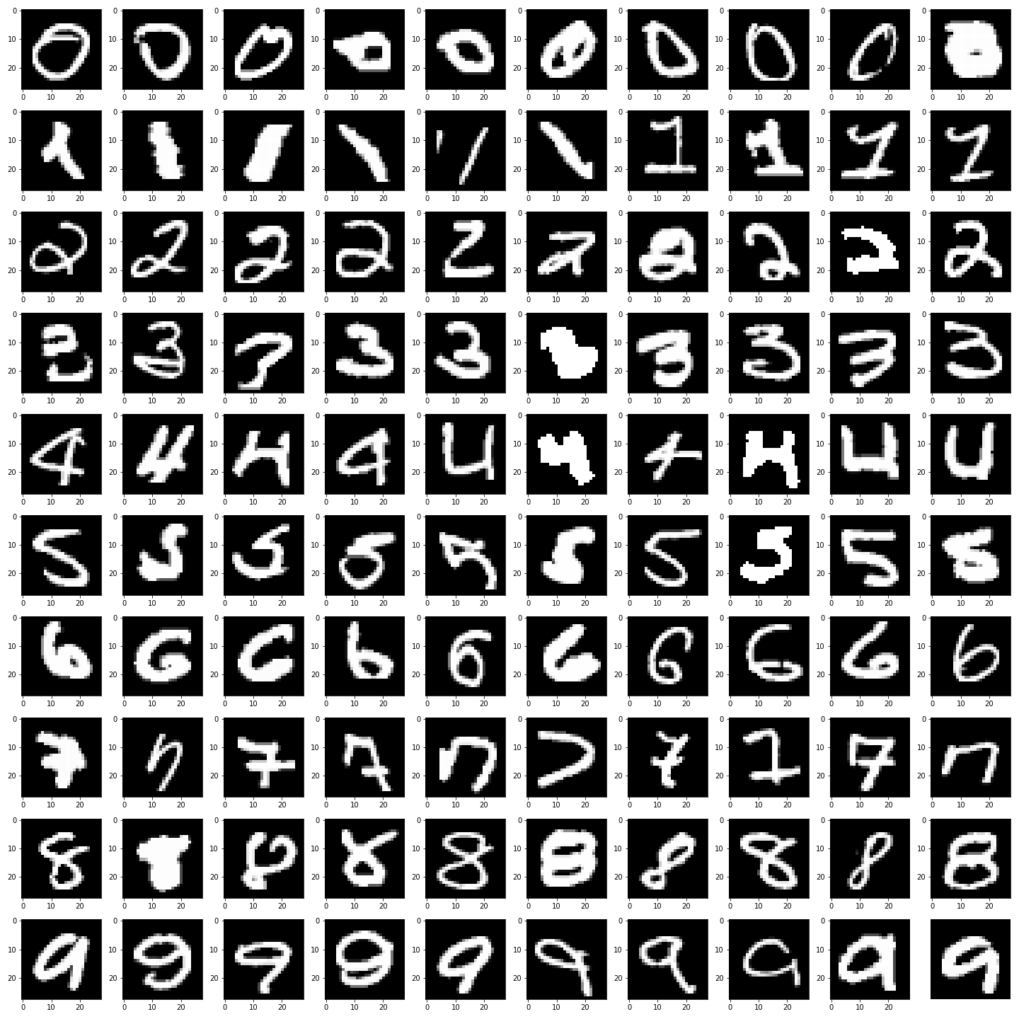
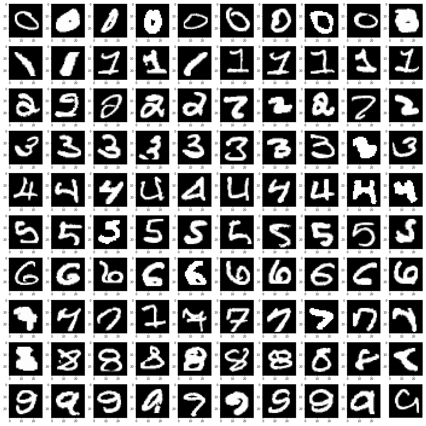
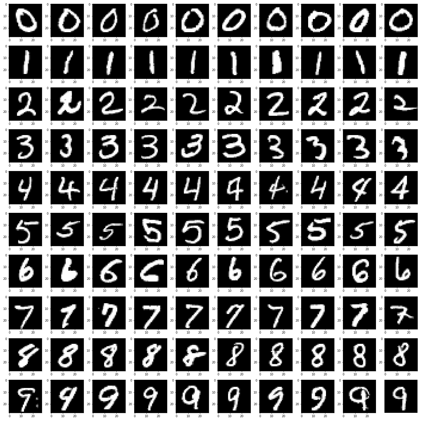
Prop. 7 applies to abstract datasets as well; we consider the MNIST dataset lecun1998mnist , treating each image as a point in $d=784$ dimensions. Here $\Gamma$ is the point set consisting of all images of the same digit. Fig. 5 shows the average digits over the whole dataset, versus the average of those sampled by RaySense.

Figure 5: Each digit averaged over the entire data set (top) versus those sampled by RaySense (bottom).

In the context of MNIST, salient points are digits that are drawn using less typical strokes (according to the data). These are the data points that may be harder to classify, since they appear less frequently in the data. RaySense may be used to determine the most useful data points to label, as in active learning settles2009active . RaySense also provides a special notion of importance sampling based on the notion of saliency described above. An application of such a property is further discussed in Sec. 4.2.

3.2.2 Invariant histogram

The relationship between the frequency of a point in $\Gamma$ being sampled and the measure of its Voronoi cell derived in Sec. 3.1.1 also provides a crucial guarantee. It ensures the RaySense histogram introduced in (11) possesses a well-defined limit as the number of rays $m\to\infty$. This convergence can be better elucidated using an alternative formulation of $H_{k}$ from (11), which incorporates the concept of Voronoi cell:

Draw $m$ rays, $\bm{r}_{1},\bm{r}_{2},\ldots,\bm{r}_{m},$ from the distribution $\mathcal{L}$ that are contained in some $B_{R}(0)$ of suitable $R$. Enumerate this set of points by $\bm{r}_{i,j}$, and the spacing between two adjacent points is given by $\delta r$. The closest point of $\bm{r}_{i,j}$ is $\bm{x}_{k}$ if $\bm{r}_{i,j}\in V_{k}:=V(\bm{x}_{k})$. Therefore, the bin value of the RaySense histogram can also be given as:

$$H_{k}=H\big{(}\bm{x}_{k}\mathchar 24635\relax\;\mathcal{S}_{m,\delta r}(\Gamma)\big{)}:=\sum_{i=1}^{m}\sum_{\bm{r}_{i,j}\in V_{k}}1,$$

where $\mathcal{S}_{m,\delta r}(\Gamma)$ denotes the closest point sketch tensor using $m$ rays and $\delta r$ spacing. The following Theorem shows that under proper normalization, $H_{k}$ can be thought as a hybrid Monte-Carlo approximation to $\mathbb{E}[\ell_{k}]$ defined in (15):

Theorem 8.

The normalized bin values $\tilde{H}_{k}$ with the normalized constant $\delta r/m$, i.e.,

$$\tilde{H}_{k}:=\frac{\delta r}{m}H\big{(}\bm{x}_{k}\mathchar 24635\relax\;\mathcal{S}_{m,\delta r}(\Gamma)\big{)}=\frac{1}{m}\sum_{i=1}^{m}\sum_{\bm{r}_{i,j}\in V_{k}}\delta r,$$

have the limit

$$\lim_{\begin{subarray}{c}\rule{0.0pt}{3.91806pt}m\rightarrow\infty\\ \rule{0.0pt}{3.91806pt}\delta r\rightarrow 0\end{subarray}}\tilde{H}_{k}(\mathcal{S}_{m,\delta r}(\Gamma))=\mathbb{E}[\ell_{k}].$$

Proof:

$$\lim_{\begin{subarray}{c}\rule{0.0pt}{3.91806pt}m\rightarrow\infty\\ \rule{0.0pt}{3.91806pt}\delta r\rightarrow 0\end{subarray}}\tilde{H}_{k}(\mathcal{S}_{m,\delta r}(\Gamma)) =\lim_{\begin{subarray}{c}\rule{0.0pt}{3.91806pt}m\rightarrow\infty\\ \rule{0.0pt}{3.91806pt}\delta r\rightarrow 0\end{subarray}}\frac{1}{m}\sum_{i=1}^{m}\sum_{\bm{r}_{i,j}\in V_{k}}\delta r=\lim_{\delta r\to 0}\mathbb{E}_{\bm{r}_{i}\sim\mathcal{L}}\Big{[}\sum_{\bm{r}_{i,j}\in V_{k}}\delta r\Big{]}$$

$$=\mathbb{E}_{\bm{r}_{i}\sim\mathcal{L}}\Big{[}\lim_{\delta r\to 0}\sum_{\bm{r}_{i,j}\in V_{k}}\delta r\Big{]}=\mathbb{E}_{\bm{r}_{i}\sim\mathcal{L}}\Big{[}\int_{\bm{r}_{i}}\chi_{V_{k}}\big{(}\bm{r}(s)\big{)}\mathrm{d}s\Big{]}=\mathbb{E}[\ell_{k}],$$

where $\chi_{V_{k}}$ is the indicator function of $V_{k}$. Interchanging order of the limit and the expectation follows from the dominated convergence theorem since $\sum_{\bm{r}_{i,j}\in V_{k}}\delta r<\chi_{V_{k}}\big{(}\bm{r}(s)\big{)}+2\delta r$.

Monte-Carlo approximations of integrals converge with a rate independent of the dimension caflisch1998monte . Consequently, for sufficiently many randomly selected rays, the histogram is essentially independent of the rays that are actually used.

Similar arguments show that the sampling of any function of the data set will be independent of the actual ray set, since the histograms are identical in the limit. More precisely, suppose $g:\bm{x}\in\Gamma\mapsto\mathbb{R}$ is some finite function, then

$$\lim_{\begin{subarray}{c}\rule{0.0pt}{3.91806pt}m\rightarrow\infty\\ \rule{0.0pt}{3.91806pt}\delta r\rightarrow 0\end{subarray}}\frac{1}{m}\sum_{i=1}^{m}\sum_{\bm{r}_{i,j}\in V_{k}}g(\bm{x}_{k})\delta r=\mathbb{E}[g(\bm{x}_{k})\ell_{k}].$$

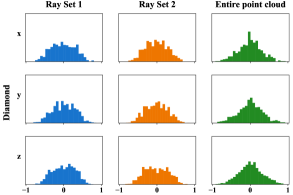
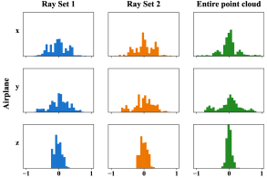
In Fig. 6, we show the histograms of the coordinates of the RaySensed points of $\Gamma$.

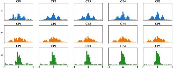
The integral $\mathbb{E}[\ell_{k}]$ (or $\mathbb{E}[g(\bm{x}_{k})\ell_{k}]$ for continuous $g$) depends smoothly on $\Gamma,$ and is therefore stable against perturbation to the coordinates of the points in $\Gamma$. However, the effect of introducing new members to $\Gamma$, such as outliers, will be non-negligible. One possible way to overcome this is to use multiple nearest neighbors for points on the rays. In Fig. 7, we show coordinates of the $\eta=5$ nearest neighbors sampled by RaySense under the presence of outliers. It is observed that the feature of the $\eta$-th nearest neighbor for $\eta$ large is more robust against outliers while also maintaining the desired histogram information. In Sec. 4.5, we will also demonstrate the effectiveness of this idea in dealing with outliers in practical tasks.

By considering a similar argument as in the proof of Thm. 4, we can provide a simple and intuitive explanation for the robustness to outliers when using more nearest neighbors: when the underlying point cloud is dense enough, if an outlier disrupts the nearest neighbor search, excluding the outlier and finding the next few nearest neighbors would mitigate the impact caused by the outlier; if an outlier does not dominate the nearest neighbor search, then the next few nearest neighbors with high probability would also originate from a small neighborhood centered around the first nearest neighbor. Therefore, increasing the number of nearest neighbors enhances the stability of RaySense.

Figure 6: Histogram of coordinates from two point sets. Columns 1 and 2 correspond to 2 different sets of rays, each containing $256$ rays and $64$ samples per ray. These histograms are similar for the same object and different for different objects. Column 3 corresponds to the entire point cloud; these differ from the RaySense histograms especially for the airplane which is not as regular as the diamond.

Figure 7: Histogram of the $\eta=5$ nearest neighbors sampled by RaySense, where the underlying point cloud is polluted by $50$ outliers uniformly sampled from the unit ball. Rows correspond to different coordinates while columns correspond to different closest points. Outliers introduce extreme values on coordinates of CP$1$ but these effects are significantly mitigated on CP$5$.

4 Examples of Applications

4.1 Comparison of histograms of RaySense samples

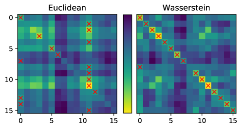
We experiment by comparing $\Gamma$ drawn from $16\,384$ objects of 16 categories from the ShapeNet dataset chang2015shapenet . Let $\beta^{i}$ be the label for object $\Gamma_{i}$. We compute the histogram $h_{x}^{i},h_{y}^{i},h_{z}^{i}$ of the $x,y,z$ coordinates, respectively, for points sampled by 50 rays with $n_{r}=10$ samples per ray. We compare the histograms against those corresponding to other objects in the dataset, using

$$D_{i,j}=d(h_{x}^{i},h_{x}^{j})+d(h_{y}^{i},h_{y}^{j})+d(h_{z}^{i},h_{z}^{j}),$$

where $d(\cdot,\cdot)$ is either the $\ell_{2}$ or Wasserstein-1 distance. We sum $D$ according to the respective labels

$$M_{a,b}\propto\sum_{i:\beta^{i}=a}\ \sum_{j:\beta^{j}=b}D_{i,j},\qquad a,b=1,\dots,16,$$

and normalize by the number of occurrences for each $a,b$ pair. Fig. 8 shows the matrix of pairwise distances $M$ between the 16 object categories.

Ideally, intra-object distances would be small, while inter-object distances would be large. As expected, Wasserstein-1 is a better metric for comparing histograms. Still, not all objects are correctly classified. When comparing histograms in not sufficient, we consider using neural networks to learn more complex mappings, such as in Sec. 4.5.

Figure 8: Comparison of histogram of the $x,y,z$ coordinates of points sampled by RaySense, using $\ell^{2}$ and the Wasserstein distance $W_{1}$. Rows and columns correspond to object labels. Red $\times$ indicate location of the argmin along each row.

4.2 Salient points in the MNIST data

From previous discussion and simulation in Sec. 3.1.1 and Sec. 3.2.1, we know RaySense has the ability to detect salient points or boundary points. Here we provide further visualization of RaySense salient points on the MNIST dataset.

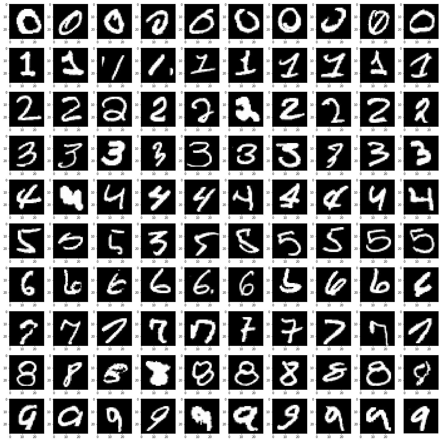
By vectorizing the MNIST image, each image is a vector in $\mathbb{R}^{784}$ with pixel value from $0$ to $255$. We generate the random ray set in this ambient space using the method R1 in Appendix A, where each ray has the fixed-length $1$, with centers uniformly shifted in the half cube $[-\frac{1}{2},\frac{1}{2}]^{784}$. Each ray set has $m=256$ random rays, with $n_{r}=64$ equi-spaced points on each ray. To ensure a good coverage over the data manifold, we rescale the MNIST image by entry-wise dividing so that each data point is constrained in an $\ell^{\infty}$ ball of a certain radius as introduced below; we also shift the dataset to have mean $0$.

As mentioned, the RaySense salient points are those in $\Gamma$ sampled most frequently by points from the rays. We record the sampling frequency for each MNIST image, and in Fig. 9b we plot the top-$10$ images with highest frequency for each class. From the figure, we see that the salient points often correspond to digits with untypical strokes and writing styles, similar to the conclusion obtained from Fig. 5. Fig. 9b further shows that different normalizations of the data (by using scaling values $2550$, $5100$ and $25500$) also affects the sampling. This phenomenon can be better understood from the perspective of truncated Voronoi cell (14): when the scale of the point clouds shrinks while the length of rays remains constant, it has a similar effect as increasing the length of the rays while keeping the point clouds unchanged, causing the truncated Voronoi cells to grow. Specifically, the truncated Voronoi cells associated with salient points exhibit a larger growth rate, as their Voronoi cells are typically unbounded, e.g. Prop. 7, making the subsampling even more biased when normalized to a smaller cube.

(a) normalized to $0.1$ cube

(b) normalized to $0.05$ cube

(c) normalized to $0.01$ cube

(d) uniformly random

Figure 9: MNIST digit images with highest RaySense sampling frequencies for each class. Three different normalizations are shown in (a), (b) and (c). Compared to a uniformly random subsample (d), we see a wider variety of hand-writing styles in the RaySense output.

.
.

4.3 RaySense and integral transforms

A line $\bm{r}$ in $\mathbb{R}^{d}$ in the direction of $\bm{\theta}\in\mathbb{S}^{d-1}$ has parameterization $\bm{r}(s)=\bm{b}+s\bm{\theta}$, $s\in(-\infty,\,\infty)$, with $\bm{b}\in\mathbb{R}^{d}$ a reference point on the line. Without loss of generality, let $\bm{b}$ be in $\bm{\theta}^{\perp}$, which is a hyperplane orthogonal to $\bm{\theta}$ passing through the origin. The X-ray transform for a non-negative continuous function $g$ with compact support Natterer:computerized_tomography_siambook is defined on the set of all lines in $\mathbb{R}^{d}$ by

$$\mathcal{X}[g](\bm{b},\bm{\theta}):=\int_{-\infty}^{\infty}g(\bm{b}+s\bm{\theta})\mathrm{d}s.$$ (20)

The spectrum of $g$ can be obtained via the Fourier slice theorem solmonXRay1976 :

$$\mathcal{F}[\mathcal{X}g](\bm{\theta},\bm{\xi})=\mathcal{F}[g](\bm{\xi}),\quad\bm{\xi}\in\bm{\theta}^{\perp}.$$

When we restrict $\bm{\xi}$ to be only on a line in $\bm{\theta}^{\perp}$, we are effectively collecting information on a $2$-dimensional slice of $g$ parallel to $\bm{\theta}^{\perp}$.

However, when the function $g$ only has a sampling representation, e.g., a point cloud, it is non-trivial to compute such integrals. In Section 3.1.3, we showed that if $\bm{r}$ is a member of the sampling ray set, one can compute an approximation of (20) from the RaySense sketch obtained from $\{\bm{x}_{k},g(\bm{x}_{k})\}_{k=1}^{N}$, where $\{\bm{x}_{k}\}$ are i.i.d. samples from a known probability density $\rho$. Thus, RaySense provides a convenient alternative in obtaining (or, in a sense, defining) the Fourier slices of the discrete data set $\{\bm{x}_{k},g(\bm{x}_{k})\}_{k=1}^{N}$. Since (20) is defined for any dimension, one can approximate the X-ray transform from a RaySense sketch using suitable ray sets, or, in the random case, RaySense integrals can be regarded as randomized approximations of X-ray transforms.

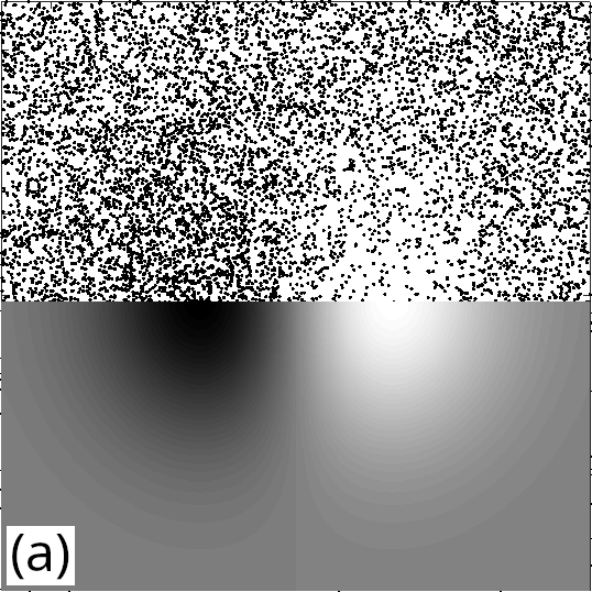
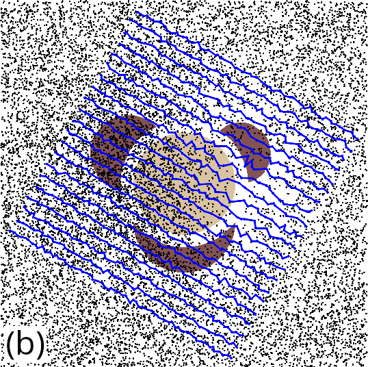
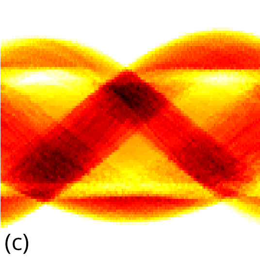
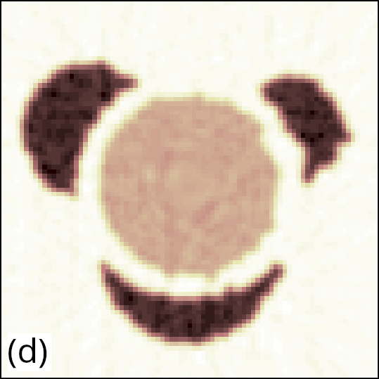
In Fig. 10 we show an example of using RaySense sampling with prescribed (rather than random) rays to approximate the Radon transform. In this experiment, a point cloud $\Gamma$ (Fig. 10(a) top) with $15010$ points, is sampled from density $\rho=\frac{1}{2}-3xe^{-9x^{2}-9y^{2}}$ (Fig. 10(a) bottom)—note denser (darker) region on left and sparser (lighter) region on right. $\Gamma$ has data shown in Fig. 10(b) evaluated from the piecewise constant function $g$, shown by the solid colours (for visualization only; $g$ is only known at the discrete points in $\Gamma$). Blue lines show the locations of the RaySense sketch for one particular angle (illustrated with 21 rays but the computation uses 100). We note increasingly jagged lines to the right where the point cloud is sparser. Fig. 10(c) shows that approximate Radon transform computed over 180 degrees in steps of one degree by integrating the RaySense sketch using trapezoidal rule at $n_{r}=64$ points per ray. Fig. 10(d) shows the filtered back projection computed by the Octave Image package OctaveImagePkg . Note a more jagged reconstruction on the right where the point cloud is sparsest. If we instead used random rays, we could generate samples at scattered points in the sinogram (Fig. 10(c)) which could then be used for an approximate inverse transform.

Figure 10: Approximate Radon transform computed with RaySense from point cloud data (a)–(c) and filtered back projection reconstruction (d).

4.4 Point cloud registration

In this section, we explore the application of RaySense to the point cloud registration problem. Given two point sets $\Gamma$ and $\tilde{\Gamma}$ in 3-d consisting of distinct points, registration aims to find the 3-d rotation matrix $\bm{U}$ and translation vector $\bm{b}$ to minimize the Euclidean norm of points in correspondence. When the correspondence is known, this is the orthogonal Procrustes problem and the solution can be obtained explicitly via the singular value decomposition. When the correspondence is unknown, one can formulate an optimization problem and solve with various carefully-designed algorithms. Here we choose to use the Iterative Closest Point (ICP) besl1992method due to its simplicity, which minimizes point-wise Euclidean distance iteratively from the optimization problem

$$\min_{\bm{U}\in SO(3),\bm{b}\in\mathbb{R}^{3}}\sum_{\bm{x}_{j}\in\tilde{\Gamma}}\min_{\bm{y}\in\Gamma}\|U(\bm{x}_{j}+\bm{b})-\bm{y}\|^{2}_{2}.$$

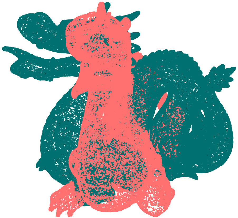
We set up the problem using the Stanford Dragon StanfordDragon_Curless96 as a point cloud $\Gamma$ with $100\,000$ points. We artificially generate the target point cloud to register by rotating by $\pi/3$ in one direction. We compare the performance of ICP in three scenarios: 1) the original dense point clouds, 2) a uniformly random subsampling (in index) of the point clouds, 3) RaySense closest point samples using $\mathcal{S}[\Gamma]$ (without repetition of sampled points) of each point cloud. Specifically, we use $m=512$ rays, each with $n_{r}=64$ sample points, to subsample the original point cloud in RaySense, which usually generates a set of around $800$ unique points. We then sample the second point cloud with a different set of rays. For fair comparison, we also subsample $800$ points in the case of uniformly random subsampling. We use the root mean square error (RMSE) as our metric, and we also record the convergence time, where the convergence criteria is a threshold of the relative RMSE. We summarize the performance results in Tab. 1, and we provide some visualization to compare the three different settings in Fig. 11.

Table 1: Sample point cloud registration result. Performances are evaluated by registration accuracy (measured by root mean squared error (RMSE)) and computation times. The statistics reported are averaged over $5$ runs. “RMSE” is evaluated over the subsampled points while “RMSE(full)” is evaluated over the original point cloud.

	number of points	RMSE	RMSE(full)	Convergence time (s)
Vanilla ICP	100 000	4.544e-06	4.544e-06	6.319
ICP + random	800	4.509e-02	3.053e-03	0.0192
ICP + RaySense	804.6	2.601e-02	1.077e-03	0.0116

(a) original dense data

(b) random sample

(c) RaySense sample

(d) original dense data

(e) random sample

(f) RaySense sample

Figure 11: Registration simulation on a rotated Stanford dragon. Top row: initial pose and sparse samples; Bottom row: registration results. Note that the visualizations (e) and (f) are obtained by applying the transformation computed from the sparse samples in (b) and (c) to the original dense point clouds.

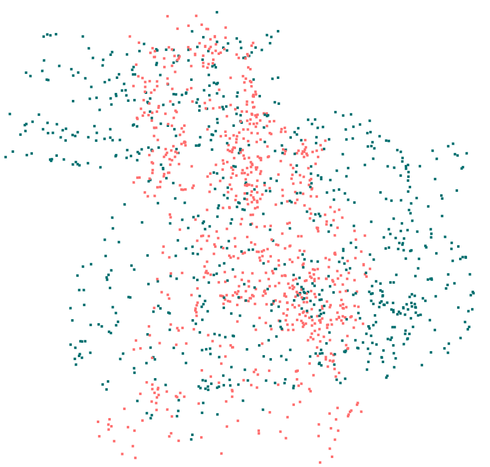
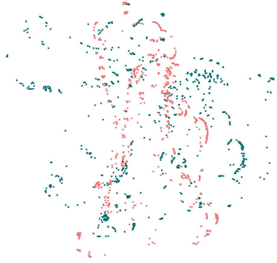
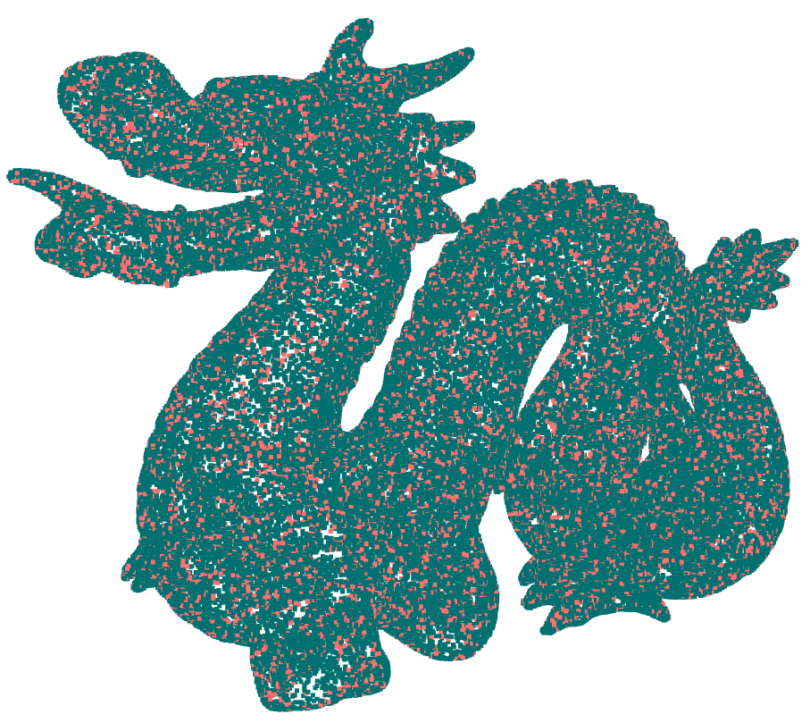
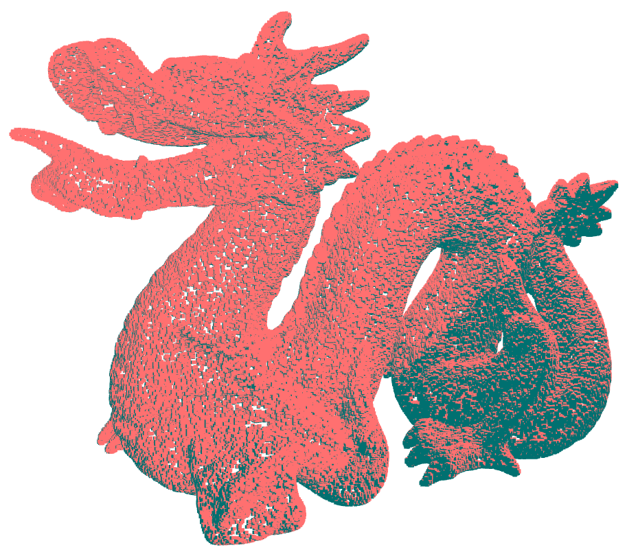
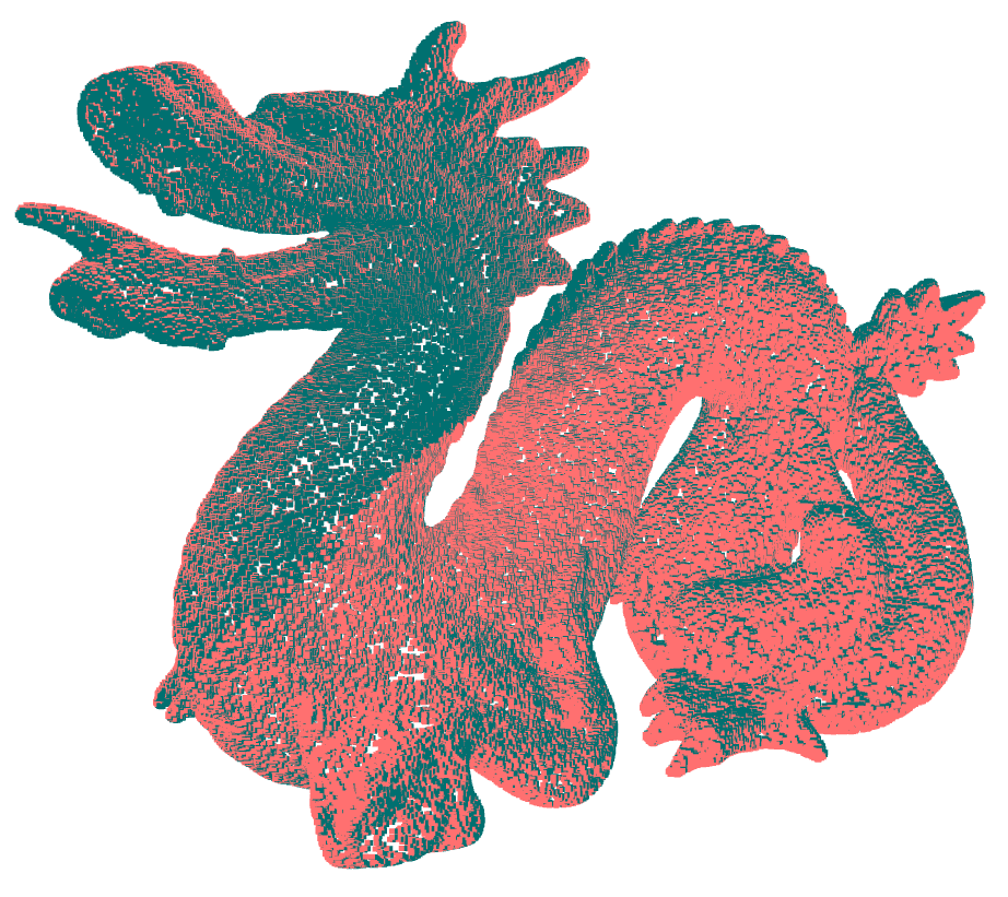
From Tab. 1, it is clear that both the sampling schemes accelerate the registration process drastically by considering only a portion of the original dense point cloud. It also suggests that RaySense sample has slight advantage over the uniform random sample, in both accuracy and convergence time. However, generating the RaySense samples on the fly needs around $0.65$s on average, while generating a random subsample requires only $0.01$s.

Fig. 11c again shows that RaySense is sampling salient features. Thus a possible improvement is to use the repetition information from RaySense sampling to perform a weighted registration, for example with the (autodetected) salient features receiving higher weights. This is left for future investigation.

4.5 Point cloud classification using neural networks

We use the RaySense sketch to classify objects from the ModelNet dataset wu20153d , using a neural network, which we call RayNN. RayNN can use features from different sampling operators $\mathcal{S}$ introduced in Sec. 2 as inputs. When using multiple nearest neighbors: $\mathcal{S}\big{[}\Gamma,[1,2,\dots,\eta]\big{]}$, we denote our models by RayNN-cp$\eta$. For our implementation, while we might use different numbers of nearest neighbors, we always include the closest point coordinates and the vector to closest points in our feature space $\mathbb{R}^{c}$ ($c\geq 6$ fixed). Details of the implementation can be found in Appendix B.

Table 2: ModelNet classification results. Here we report our best accuracy results over all experiments. For reference, the test scores for RayNN-cp5 $(m=32)$ has mean around $90.31\%$ and standard deviation around $0.25\%$ over $600$ tests.

	ModelNet10	ModelNet40
PointNet qi2017pointnet	–	89.2
PointNet++ qi2017pointnet++	–	90.7
ECC simonovsky2017dynamic	90.8	87.4
kd-net klokov2017escape	93.3	90.6
PointCNN li2018pointcnn	–	92.5
PCNN atzmon2018point	94.9	92.3
DGCNN wang2019dynamic	–	92.9
RayNN-cp1 ($m=16$)	94.05	90.84
RayNN-cp5 ($m=32$)	95.04	90.96

We compare with some well-known methods for 3D point cloud classification tasks. In addition to the results reported by qi2017pointnet , we also compare against PointNet.pytorch, a PyTorch re-implementation site:PointNetpytorch of PointNet. In all our experiments, we report overall accuracy. Table 2 shows RayNN is competitive. To investigate the robustness of our network, we perform several more experiments.

Figure 12: Testing DGCNN wang2019dynamic , PointNet qi2017pointnet and RayNN on ModelNet40 with missing data.

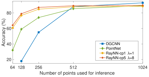
Robustness to sample size   We repeat the experiments in qi2017pointnet ; wang2019dynamic whereby, after training, data is randomly removed prior to testing on the remaining points. The results in Fig. 12 show that RayNN performs very well with significant missing data.

Using fewer rays   We experiment with training using a full set of $m=32$ rays but test using smaller number $\hat{m}$ of rays. Table 3 shows that RayNN can achieve a reasonable score even if only $\hat{m}=4$ rays are used for inference.

Robustness to outliers   This experiment simulates situations where noise severely perturbs the original data during testing. We compare the performance of RayNN-cp1, RayNN-cp5 and PointNet.pytorch in Table 4. The comparison reveals RaySense’s capability in handling unexpected outliers, especially when additional nearest neighbors are used. Note the experiment here is different from that in qi2017pointnet where the outliers are fixed and included in the training set.

Table 3: Accuracy when testing with a reduced ray set. RayNN-cp1 was trained using $m=32$ rays. Results averaged over 5 runs.

ModelNet40
$\hat{m}$	$32$	$16$	$8$	$4$
$\lambda=1$	88.50%	86.13%	74.64%	43.28%
$\lambda=8$	89.77%	88.94%	82.97%	55.24%

Comparison of model complexity

Table 5 shows that our network has an advantage in model size and feed-forward time even against the simple and efficient PointNet. In both training and testing, there is some overhead in data preprocessing to build a kd-tree, generate rays, and perform the nearest-neighbor queries to form the RaySense sketch. For point clouds of around $N=1024$, these costs are not too onerous in practice as shown in table 5.

The convolution layers have $48c+$840\,016$$ parameters, where $c$ is the dimension of input feature space. The fully-connected layers have $64K+$278\,528$$ parameters, where $K$ is the number of output classes. In total, our network has $1.1\times 10^{6}+48c+64K\approx 1.1$M parameters. In comparison, PointNet qi2017pointnet contains $3.5$M parameters.

Table 4: Outliers sampled uniformly from the unit sphere are introduced during testing. The networks are trained without any outliers. Results averaged over 5 runs.

ModelNet10	no outliers	5 outliers	10 outliers
RayNN-cp1	93.26%	79.76%	53.94%
RayNN-cp5	93.85%	92.66%	90.90%
PointNet.pytorch​​	91.08%	48.57%	25.55%
ModelNet40
RayNN-cp1	89.77 %	54.66%	20.95%
RayNN-cp5	90.38%	88.49%	78.06%
PointNet.pytorch​​	87.15%	34.05%	17.48%

Table 5: Top: storage and timings for RayNN-cp1 and PointNet.pytorch on ModelNet40 using one Nvidia 1080-Ti GPU and batch size 32. The preprocessing and forward time are both measured per batch. Bottom: data from wang2019dynamic is included only for reference; no proper basis for direct comparison.

	Model size	Forward time	Preprocessing time	Time per epoch
PointNet.pytorch​​	$14\text{\,}\mathrm{M}\mathrm{B}$	$12\text{\,}\mathrm{m}\mathrm{s}$	3.6 $\mathrm{m}\mathrm{s}$	14 $\mathrm{s}$
RayNN-cp1	4.5 $\mathrm{M}\mathrm{B}$	2 $\mathrm{m}\mathrm{s}$	$7.5\text{\,}\mathrm{m}\mathrm{s}$	$22\text{\,}\mathrm{s}$
PointNet qi2017pointnet	$40\text{\,}\mathrm{M}\mathrm{B}$	$16.6\text{\,}\mathrm{m}\mathrm{s}$	-	-
PCNN atzmon2018point	$94\text{\,}\mathrm{M}\mathrm{B}$	$117\text{\,}\mathrm{m}\mathrm{s}$	-	-
DGCNN wang2019dynamic	$21\text{\,}\mathrm{M}\mathrm{B}$	$27.2\text{\,}\mathrm{m}\mathrm{s}$	-	-

5 Summary

RaySense is a sampling technique based on projecting random rays onto a data set. This projection involves finding the nearest neighbors in the data for points on the rays. These nearest neighbors collectively form the basic “RaySense sketch”, which can be employed for various data processing tasks.

RaySense does not merely produce narrowly interpreted subsamples of given datasets. Instead, it prioritizes the sampling of salient features of the dataset, such as corners or edges, with a higher probability. Consequently, points near these salient features may be recorded in the sketch tensor multiple times.

From the RaySense sketch, one can further extract snapshots of integral or local (differential) information about the data set. Relevant operations are defined on the rays randomly sampled from a chosen distribution. Since rays are one-dimensional objects, the formal complexity of RaySense does not increase exponentially with the dimensions of the embedding space. We provide theoretical analysis showing that the statistics of a sampled point cloud depends solely on the distribution of the rays, and not on any particular ray set. Additionally, we also demonstrated that by appropriately post-processing the RaySense sketch tensor obtained from a given point cloud, one can compute approximations of line integrals. Thus, and by way of the Fourier Slice Theorem, we argue that RaySense provides spectral information about the sampled point cloud.

We showed that RaySense sketches could be used to register and classify point clouds of different cardinality. For classification of point clouds in three dimensions, we presented a neural network classifier called “RayNN”, which takes the RaySense sketches as input. Nearest-neighbor information can be sensitive to outliers. For finite point sets, we advocated augmentation of the sketch tensor by including multiple nearest neighbors to enhance RaySense’s capability to capture persistent features in the data set, thereby improving robustness. We compared the performance of RayNN to several other prominent models, highlighting its lightweight, flexible, and efficient nature. Importantly, RayNN also differs from conventional models, as it allows for multiple tests with different ray sets on the same dataset.

Acknowledgments   Part of this research was performed while Macdonald and Tsai were visiting the Institute for Pure and Applied Mathematics (IPAM), which is supported by the National Science Foundation (Grant No. DMS-1440415). This work was partially supported by a grant from the Simons Foundation, NSF Grants DMS-1720171 and DMS-2110895, and a Discovery Grant from Natural Sciences and Engineering Research Council of Canada. The authors thank Texas Advanced Computing Center (TACC) and UBC Math Dept Cloud Computing for providing computing resources.

Statements and Declarations   The authors have no competing interests to declare that are relevant to the content of this article.

Appendix A Examples of ray distributions

We assume all points are properly calibrated by a common preprocessing step. This could also be learned. In fact, one can use RaySense to train such a preprocessor to register the dataset, for example, using Sec. 4.4 or similar. However, for simplicity, in our experiments, we generally normalize each point set to be in the unit $\ell^{2}$ ball, with center of mass at the origin, unless otherwise indicated.

We present two ways to generate random rays. There is no right way to generate rays, although it is conceivable that one may find optimal ray distributions for specific applications.

Method R1   One simple approach is generating rays of fixed-length $L$, whose direction $\bm{v}$ is uniformly sampled from the unit sphere. We add a shift $\bm{b}$ sampled uniformly from $[-\frac{1}{2},\frac{1}{2}]^{d}$ to avoid a bias for the origin. The $n_{r}$ sample points are distributed evenly along the ray:

$$\bm{r}_{i}=\bm{b}+L\left(\frac{i}{n_{r}-1}-\frac{1}{2}\right)\bm{v},\qquad i=0,\dots,n_{r}-1$$

The spacing between adjacent points on each ray is denoted by $\delta r$, which is $L/(n_{r}-1)$. We use $L=2$.

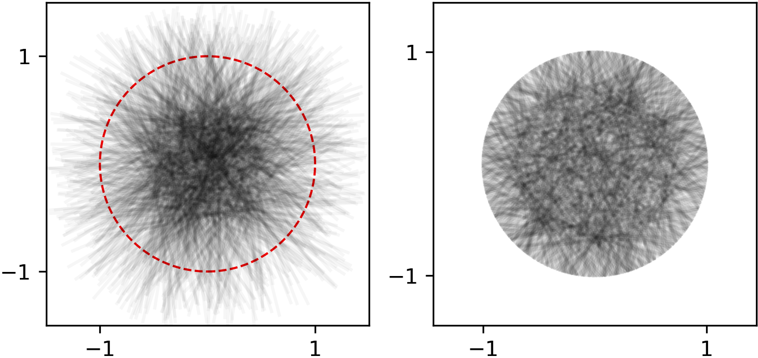
Method R2   Another natural way to generate random rays is by random endpoints selection: choose two random points $\bm{p}$, $\bm{q}$ on a sphere and connect them to form a ray. Then we evenly sample $n_{r}$ points between $\bm{p}$, $\bm{q}$ on the ray. To avoid overly short rays where information would be redundant, we use a minimum ray-length threshold $\tau$ to discard rays. Note that the distance between $n_{r}$ sample points are different on different rays:

$$\bm{r}_{i}=\bm{p}+\frac{i}{n_{r}-1}(\bm{q}-\bm{p}),\qquad i=0,\dots,n_{r}-1.$$

The spacing of points on each ray varies, depending on the length of the ray.

Fig. 13 shows the density of rays from the ray generation methods. In this paper, we use Method R1; a fixed $\delta r$ seems to help maintain spatial consistency along the rays, which increases RayNN’s classification accuracy in Sec. 4.5.

Figure 13: Density of rays from method R1 (left) and R2 (right). Red circle indicates the $\ell^{2}$ ball.

Appendix B Implementation details of RayNN

Our implementation uses PyTorch paszke2017automatic .

Architecture   RayNN takes the $m\times k\times c$ RaySense sketch tensor $\mathcal{S}(\Gamma)$ as input, and outputs a $K$-vector of probabilities, where $K$ is the number of object classes.

The first few layers of the network are blocks of 1D convolution followed by max-pooling to encode the sketch into a single vector per ray. Convolution and max-pooling are applied along the ray. After this downsizing, we implement a max operation across rays. Fig. 14 includes some details. The output of the max pooling layer is fed into fully-connected layers with output sizes $256$, $64$, and $K$ to produce the desired vector of probabilities $\bm{\mathbf{p}}_{i}\in\mathbb{R}^{K}$. Batchnorm ioffe2015batch along with ReLU nair2010rectified are used for every fully-connected and convolution layer.

Note that our network uses convolution along rays to capture local information while the fully-connected layers aggregate global information. Between the two, the max operation across rays ensures invariance to the ordering of the rays. It also allows for an arbitrary number of rays to be used during inference. These invariance properties are similar to PointNet’s input-order invariance qi2017pointnet .

Figure 14: The RayNN architecture for $m$ rays and $n_{r}$ samples per ray. The input is $c$ feature matrices from $\mathcal{S}(\Gamma)$ with suitable operations. With $n_{r}=16$, each matrix is downsized to an $m$-vector by 4 layers of 1-D convolution and max-pooling. The max operator is then applied to each of the 1024 $m$-vectors. The length-$1024$ feature vector is fed into a multi-layer perceptron (mlp) which outputs a vector of probabilities, one for each of the $K$ classes in the classification task. Note the number of intermediate layers (blue) can be increased based on $n_{r}$ and $c$.

Data   We apply RayNN on the standard ModelNet10 and ModelNet40 benchmarks wu20153d for 3D object classification. ModelNet40 consists of $12\,311$ orientation-aligned sedaghat2016orientation meshed 3D CAD models, divided into $9843$ training and $2468$ test objects. ModelNet10 contains $3991$ training and $908$ test objects. Following the experiment setup in qi2017pointnet , we sample $N=1024$ points from each of these models and rescale them to be bounded by the unit sphere to form point sets. Our results do not appear to be sensitive to $N$.

Training   During training, we use dropout with ratio $0.5$ on the penultimate fully-connected layer. We also augment our training dataset on-the-fly by adding $\mathcal{N}(0,0.0004)$ noise to the coordinates. For the optimizer, we use Adam kingma2014adam with momentum $0.9$ and batch size $16$. The learning rate starts at $0.002$ and is halved every $100$ epochs.

Inference   Our algorithm uses random rays, so it is natural to consider strategies to reduce the variance in the prediction. We consider one simple approach during inference by making an ensemble of predictions from $\lambda$ different ray sets. The ensemble prediction is based on the average over the $\lambda$ different probability vectors $\vec{\mathbf{p}}_{i}\in\mathbb{R}^{K}$, i.e.,

$$\text{Prediction}(\lambda)=\frac{1}{\lambda}\sum_{i=1}^{\lambda}\vec{\mathbf{p}}_{i}.$$

The assigned label then corresponds to the entry with the largest probability. We denote the number of rays used during training by $m$, while the number of rays used for inference is $\hat{m}$. Unless otherwise specified, we use $\lambda=8$, $m=32$ rays, and $\hat{m}=m$.

Appendix C Details of the proof of Theorem 4

This appendix contains the proofs of Lemmas 1, 2, and 3, and Theorem 4.

Proof: [Proof of Lemma 1.] The probability measure of $\Omega_{j}$ is

$$P_{\Omega_{j}}=\int_{\bm{x}\in\Omega_{j}}\rho(\bm{x})\mathrm{d}\bm{x}>0,$$

which represents the probability of sampling $\Omega_{j}$ when drawing $i.i.d.$ random samples from $\mu$. For a fixed set of such hypercubes, any $\bm{x}\in\textrm{supp}(\rho)$ will fall in one of the $\Omega_{j}$’s. Then one can define a mapping $h:\textrm{supp}(\rho)\subset\mathbb{R}^{d}\to\mathbb{R}$ by:

$$s=h(\bm{x})=j-1,\quad\text{where }\bm{x}\in\Omega_{j},\;j=\,1,\,2,\,\dots,\,M.$$

By applying the mapping to the random vector $\bm{X}$, we obtain a new discrete random variable $S$ with the discrete probability distribution $\mu_{M}$ on $\mathbb{R}$ and the corresponding density $\rho_{M}$. The random variable $S$ lives in a discrete space: $S\in\{0,\,1,\,\ldots,\,M-1\}$ and $\rho_{M}$ is given as a sum of delta spikes as

$$\rho_{M}(s)=\sum_{j=1}^{M}P_{\Omega_{j}}\delta_{j}(s).$$

As a result, sampling from the distribution $\mu_{M}$ is equivalent to sampling the hypercubes according to the distribution $\mu$ in $\mathbb{R}^{d}$, but one cares only about the sample being in a specific hypercube $\Omega_{j}$, not the precise location of the sample. Let $F_{M}(s)$ denote the cumulative density function related to the density function $\rho_{M}(s)$.

Now, given a set of $N$ independent samples of $\bm{X}:$ $\{\bm{X}_{i}\}_{i=1}^{N}\subset\mathbb{R}^{d}$, we have a corresponding set of $N$ independent sample points of $S:$ $\{s_{i}\}_{i=1}^{N}$ such that $\bm{X}_{i}\in\Omega_{s_{i}+1}$. From there, we can regard the histogram of $\{s_{i}\}_{i=1}^{N}$ as an empirical density of the true density $\rho_{M}$. Denote the empirical density by $\tilde{\rho}_{M}^{N}$ which is given by

$$\tilde{\rho}_{M}^{N}=\frac{1}{N}\sum_{i=1}^{N}\delta_{s_{i}}.$$

one can therefore also obtain an empirical cumulative density function $\tilde{F}^{N}_{M}(s)$ using the indicator function $\chi$:

$$\tilde{F}^{N}_{M}(s)=\frac{1}{N}\sum_{i=1}^{N}\chi_{\{s_{i}\leq s\}}.$$

By Dvoretzky–Kiefer–Wolfowitz inequality dvoretzky1956asymptotic ; massart1990tight we have

$$Prob\big{(}\sup_{s\in\mathbb{R}}\lvert F_{M}(s)-\tilde{F}^{N}_{M}(s)\rvert>\varepsilon\big{)}\leq 2e^{-2N\varepsilon^{2}},\quad\text{ for all }\varepsilon>0.$$

Therefore, for a desired fixed probability $p_{0}$, the above indicates the approximating error given by the empirical $\tilde{F}^{N}_{M}(s)$ is at most

$$\sup_{s\in\mathbb{R}}\lvert F_{M}(s)-\tilde{F}^{N}_{M}(s)\rvert\leq\varepsilon_{N}=\Big{(}-\frac{1}{2N}\ln{\big{(}\frac{1-p_{0}}{2}\big{)}}\Big{)}^{\frac{1}{2}},$$

with probability at least $p_{0}$. Then note that the true probability measure $P_{\Omega_{j}}$ of $\Omega_{j}$ being sampled by random drawings from $\mu$ is equivalent to the true probability of $j-1$ being drawn from $\mu_{M}$, $i.e.$

$$P_{\Omega_{j}}=P_{M}(j-1):=\rho_{M}(j-1),$$

therefore $P_{\Omega_{j}}=P_{M}(j-1)$ can be computed from $F_{M}$ by:

$$P_{\Omega_{j}} =F_{M}(j-1)-F_{M}(j-2)$$

$$=F_{M}(j-1)-\tilde{F}^{N}_{M}(j-1)+\tilde{F}^{N}_{M}(j-1)-\tilde{F}^{N}_{M}(j-2)+\tilde{F}^{N}_{M}(j-2)-F_{M}(j-2).$$

Taking absolute value and using the triangle inequality, with the fixed $p_{0}$

$$P_{\Omega_{j}}\leq 2\varepsilon_{N}+\tilde{P}^{N}_{M}(j-1),$$

where $\tilde{P}^{N}_{M}(j-1)$ denotes the empirical probability at $j-1$. Apply the same argument to $\tilde{P}^{N}_{M}(j-1)$ one has

$$\lvert P_{\Omega_{j}}-\tilde{P}^{N}_{M}(j-1)\rvert\leq 2\varepsilon_{N},\quad\text{for all }j=1,\,2,\,\dots,\,M.$$

For a set of $N$ sample points, $\tilde{P}^{N}_{M}(j-1)$ is computed by $\displaystyle\frac{N_{j}}{N}$, where $N_{j}$ is the number of times $j-1$ got sampled by $\{s_{i}\}_{i=1}^{N}$, or equivalently $\Omega_{j}$ got sampled by $\{\bm{X}_{i}\}_{i=1}^{N}$, which indicates that in practice, with probability at least $p_{0}$, the number of sampling points $N_{j}$ in $\Omega_{j}$ satisfies the following bound:

$$P_{\Omega_{j}}-2\varepsilon_{N}\leq\frac{1}{N}N_{j}\leq P_{\Omega_{j}}+2\varepsilon_{N}\implies P_{\Omega_{j}}N-2\varepsilon_{N}N\leq N_{j}\leq P_{\Omega_{j}}N+2\varepsilon_{N}N.$$

By taking $N$ large enough such that $P_{\Omega_{j}}N-2\varepsilon_{N}N=1\implies N_{j}\geq 1$:

$$\implies N=\frac{\sqrt{\ln{(\frac{1-p_{0}}{2})}\big{(}\ln{(\frac{1-p_{0}}{2})}-2P_{\Omega_{j}}\big{)}}+P_{\Omega_{j}}-\ln{(\frac{1-p_{0}}{2})}}{P_{\Omega_{j}}^{2}}.$$

The above quantity is clearly a function with respect to the probability measure $P_{\Omega_{j}}$, and any $\Omega_{i}$ with $P_{\Omega_{i}}\geq P_{\Omega_{j}}$ would have $N_{i}\geq N_{j}\geq 1$. Using $\nu$ to denote such a function and $0<P\leq 1$ as the threshold measure completes the first part of the proof:

$$\implies\nu\big{(}P\big{)}=\frac{\sqrt{\ln{(\frac{2}{1-p_{0}})}\big{(}\ln{(\frac{2}{1-p_{0}})}+2P\big{)}}+P+\ln{(\frac{2}{1-p_{0}})}}{P^{2}}.$$

To establish the bounds on the expression, we note

$$\nu(P) >\frac{\sqrt{\ln{(\frac{2}{1-p_{0}})}\ln{(\frac{2}{1-p_{0}})}}+P+\ln{(\frac{2}{1-p_{0}})}}{P^{2}}=\frac{2\ln{(\frac{2}{1-p_{0}})}+P}{P^{2}},$$

$$\nu(P) <\frac{\sqrt{\big{(}\ln{(\frac{2}{1-p_{0}})}+2P\big{)}^{2}}+P+\ln{(\frac{2}{1-p_{0}})}}{P^{2}}=\frac{2\ln{(\frac{2}{1-p_{0}})}+3P}{P^{2}}.$$

Proof: [Proof of Lemma 2.] Consider a local hypercube centered at $\bm{y}$, $\Omega_{\bm{y}}:=\{\bm{x}+\bm{y}\in\mathbb{R}^{d}:\|\bm{x}\|_{\infty}=l/2\}$ of length $l$ to be determined. We shall just say “cube.” The probability of cube $\Omega_{\bm{y}}$ being sampled is given by $P_{\Omega_{\bm{y}}}=\int_{\Omega_{\bm{y}}}\rho(\bm{x})\mathrm{d}\bm{x}$. Now for the set of standard basis vector $\{\bm{e}_{i}\}_{i=1}^{d}$, let $\bm{v}_{d}$ denotes the sum of all the basis: $\bm{v}_{d}:=\sum_{i=1}^{d}\bm{e}_{i}$. Without loss of generality, the probability of a diagonal cube, defined by $\Omega_{\bm{y}_{d}}:=\{\bm{x}+\bm{y}+\bm{v}_{d}\in\mathbb{R}^{d}:\|\bm{x}\|_{\infty}=l/2\}$, being sampled (unconditional to $\Omega_{\bm{y}}$ being sampled) has the following bound by Lipschitz continuity of $\rho$:

$$\lvert P_{\Omega_{\bm{y}_{d}}}-P_{\Omega_{\bm{y}}}\rvert\leq\int_{\Omega_{\bm{y}}}\lvert\rho(\bm{x}+l\bm{v}_{d})-\rho(\bm{x})\rvert\mathrm{d}\bm{x}\leq L\sqrt{d}\,l\lvert\Omega_{\bm{y}}\rvert\implies P_{\Omega_{\bm{y}_{d}}}\geq P_{\Omega_{\bm{y}}}-L\sqrt{d}\,l^{d+1}.$$

Furthermore, $P_{\Omega_{\bm{y}}}$ has the following lower bound also by Lipschitz continuity of $\rho$. For any $x\in\Omega_{\bm{y}}$, we have:

$$\lvert\rho(\bm{x})-\rho(\bm{y})\rvert\leq L\sqrt{d}\frac{l}{2}\implies\rho(\bm{x})\geq\rho(\bm{y})-L\frac{\sqrt{d}}{2}l\implies P_{\Omega_{\bm{y}}}\geq\big{(}\rho(\bm{y})-L\frac{\sqrt{d}}{2}l\big{)}l^{d}.$$ (21)

Combining with the previous bound for $P_{\Omega_{\bm{y}_{d}}}$, we further have:

$$P_{\Omega_{\bm{y}_{d}}}\geq\big{(}\rho(\bm{y})-L\frac{\sqrt{d}}{2}l\big{)}l^{d}-L\sqrt{d}l^{d+1}=\rho(\bm{y})l^{d}-\frac{3\sqrt{d}}{2}Ll^{d+1}.$$

By setting $\rho(\bm{y})>\frac{3\sqrt{d}}{2}Ll$ we can ensure $P_{\Omega_{\bm{y}_{d}}}>0$, but this extreme lower bound is based on on Lipschitz continuity. To obtain a more useful bound, we will show below that by picking $l:=l_{N}$ judiciously, $\rho(\bm{y})>3\sqrt{d}Ll_{N}>0$, any surrounding cube has non-zero probability to be sampled. Therefore, with $\rho(\bm{y})>3\sqrt{d}Ll_{N}$, for any diagonal cube $\Omega_{y_{d}}$:

$$\rho(\bm{y})l^{d}-\frac{1}{2}\rho(\bm{y})l^{d}>\frac{3\sqrt{d}}{2}Ll^{d+1}\implies P_{\Omega_{\bm{y}_{d}}}>\frac{1}{2}\rho(\bm{y})l_{N}^{d}.$$

Since the diagonal cube is the furthest to $\bm{y}$ among all the surrounding cubes, we have for every surrounding cube of $\Omega_{\bm{y}}$, their probability measure is at least $P_{\Omega_{\bm{y}_{d}}}$

According to Lemma 1, for $N$ sampling points, with probability at least $p_{0}$, if a region has probability measure $\geq P_{N}$, then there is at least one point sampled in that region, where $P_{N}$ is the threshold probability depending on $N$ obtained by solving the equation below:

$$N=\frac{\sqrt{\ln{(\frac{2}{1-p_{0}})}\big{(}\ln{(\frac{2}{1-p_{0}})}+2P_{N}\big{)}}+P_{N}+\ln{(\frac{2}{1-p_{0}})}}{(P_{N})^{2}}.$$

By the bounds for $N$ in (17) of Lemma 1, we know there is some constant $c\in(1,3)$ $s.t.$:

$$N=\frac{2\ln{(\frac{2}{1-p_{0}})}+cP_{N}}{P_{N}^{2}}\implies NP_{N}^{2}-cP_{N}-2\ln{(\frac{2}{1-p_{0}})}=0.$$

Solving the above quadratic equation and realize that $P_{N}>0$, we have

$$P_{N}=\frac{c+\big{(}c^{2}+8N\ln{(\frac{2}{1-p_{0}})}\big{)}^{1/2}}{2N}.$$

Therefore, for a fixed $N$, by requiring

$$P_{\Omega_{\bm{y}_{d}}}>\frac{\rho(\bm{y})}{2}l_{N}^{d}\geq P_{N}\implies l_{N}\geq\Big{(}\frac{c+\big{(}c^{2}+8N\ln{(\frac{2}{1-p_{0}})}\big{)}^{1/2}}{\rho(\bm{y})N}\Big{)}^{\frac{1}{d}},$$

we have with probability $p_{0}$ that at every surrounding cube of $\Omega_{\bm{y}}$ of side length $l_{N}$, there is at least one point. This lower bound for $l_{N}$ ensures the surrounding cube has enough probability measure to be sampled. Since $1<c<3$, we can just take $l_{N}$ to be:

$$l_{N}:=\Big{(}\frac{3+\big{(}9+8N\ln{(\frac{2}{1-p_{0}})}\big{)}^{1/2}}{\rho(\bm{y})N}\Big{)}^{\frac{1}{d}}>\Big{(}\frac{c+\big{(}c^{2}+8N\ln{(\frac{2}{1-p_{0}})}\big{)}^{1/2}}{\rho(\bm{y})N}\Big{)}^{\frac{1}{d}}.$$

From above we see that for a fixed $\rho(\bm{y})$, $l_{N}$ decreases as $N$ increases. Therefore, by choosing $N$ large enough, we can always satisfy the prescribed assumption $\rho(\bm{y})\geq 3\sqrt{d}Ll_{N}$.

Furthermore, when $N$ is so large such that $\rho(\bm{y})\geq 3\sqrt{d}Ll_{N}$ is always satisfied, we see that $l_{N}$ is a decreasing function of $\rho$, meaning that with a higher local density $\rho(\bm{y})$, the $l_{N}$ can be taken smaller while the sampling statement still holds, meaning the local region is more compact.

Finally, since there is a point in every surrounding cube of $\Omega_{\bm{y}}$, the diameter of the Voronoi cell of $\bm{y}$ has the following upper-bound with the desired probability $p_{0}$:

$$\textrm{diam}(V(\bm{y}))\leq 3l\sqrt{d}=3\sqrt{d}\Big{(}\frac{3+\big{(}9+8N\ln{(\frac{2}{1-p_{0}})}\big{)}^{1/2}}{\rho(\bm{y})N}\Big{)}^{\frac{1}{d}}.$$

Now, for a sample point $x_{0}$ in the interior of $\textrm{supp}(\rho)$, given a cover of cubes as in Lemma 1, $x_{0}$ must belong to one of the cubes with center also denoted by $\bm{y}$ with a slight abuse of notation. Then note that the diameter of $V(\bm{x}_{0})$ also has the same upper bound as shown above. To go from $\rho(\bm{y})$ to $\rho(\bm{x}_{0})$, by Lipschitz continuity: $\rho(\bm{y})\geq\rho(\bm{x}_{0})-\frac{L\sqrt{d}}{2}l_{N}\implies\rho(\bm{x}_{0})\leq\rho(\bm{y})+\frac{L\sqrt{d}}{2}l_{N}$. Since we require $\rho(\bm{y})\geq 3\sqrt{d}Ll_{N}$, we have $\rho(\bm{x}_{0})\leq\frac{\rho(\bm{y})}{6}+\rho(\bm{y})=\frac{7}{6}\rho(\bm{y})$. Therefore:

$$\rho(\bm{y})\geq\frac{6}{7}\rho(\bm{x}_{0})\implies\textrm{diam}(V(\bm{x}_{0}))\leq 3\sqrt{d}\Big{(}\frac{21+7\big{(}9+8N\ln{(\frac{2}{1-p_{0}})}\big{)}^{1/2}}{6\rho(\bm{x})N}\Big{)}^{\frac{1}{d}}.$$

Proof: [Proof of Lemma 3.] Without loss of generality, we assume that $\lvert\textrm{supp}(\rho)\rvert=1$, then $\rho=1$ everywhere within its support. We partition $\textrm{supp}(\rho)$ into $M$ regions such that each region has probability measure $\frac{1}{M}$. This partition can be constructed in the following way: for most of the interior of $\textrm{supp}(\rho)$, subdivide into hypercubes $\Omega_{j}$’s of the same size such that $P_{\Omega_{j}}=\frac{1}{M}$ and $\Omega_{j}$’s are contained completely inside $\textrm{supp}(\rho)$. Then the length of the hypercube, $l$, is determined by $l^{d}/\lvert\textrm{supp}(\rho)\rvert=1/M\implies l=(1/M)^{1/d}$. For the remaining uncovered regions of $\textrm{supp}(\rho)$, cover with some small cubes of appropriate sizes and combine them together to obtain a region with measure $\frac{1}{M}$.

Then, following a similar idea from Lemma 2, one has a discrete sampling problem with equal probability for each candidate, which resembles the coupon collector problem. The probability $p(N,d,M)$ that each of the $M$ region contains at least one sample point has a well-known lower bound doerr2020probabilistic :

$$p(N,d,M)\geq 1-Me^{-\frac{N}{M}}.$$

With the probability $p(N,d,M)$ given above, for an interior hypercube we again have there is at least one sample in each of its surrounding hypercube, since now there is at least one sample in each of the $M$ region. Then the Voronoi diameter for each point is at most $3l\sqrt{d}$. Fixing a desired probability $p_{0}$, we want to determine the number of regions $M$ to get a control on $l$. We need to have a bound as follows:

$$p\geq 1-Me^{-\frac{N}{M}}\geq p_{0}\implies 0<Me^{-\frac{N}{M}}\leq 1-p_{0}.$$ (22)

By rearranging, the above equality holds only when

$$\frac{N}{M}e^{\frac{N}{M}}=\frac{N}{1-p_{0}}.$$

The above equation is solvable by using the Lambert $W$ function:

$$M=\frac{N}{W_{0}\big{(}\frac{N}{1-p_{0}})}.$$

where $W_{0}$ is the principal branch of the Lambert $W$ function. Note that the Lambert $W$ function satisfies

$$W_{0}(x)e^{W_{0}(x)}=x\implies\frac{x}{W_{0}(x)}=e^{W_{0}(x)}.$$

Plug in the above identity, one has

$$\frac{M}{1-p_{0}}=\frac{N}{(1-p_{0})W_{0}\big{(}\frac{N}{1-p_{0}})}\implies M=(1-p_{0})e^{W_{0}(\frac{N}{1-p_{0}}\big{)}}.$$

Also note that the function $Me^{-\frac{N}{M}}$ is monotonically increasing in $M$ (for $M>0$), so for the bound in (22) to hold we require:

$$M\leq(1-p_{0})e^{W_{0}(\frac{N}{1-p_{0}})}.$$

By taking the largest possible integer $M$ satisfying the above inequality, we then have

$$l=(1/M)^{1/d}=\big{(}\lfloor(1-p_{0})e^{W_{0}(\frac{N}{1-p_{0}})}\rfloor)^{-1/d},$$

for every hypercube contained in $\textrm{supp}(\rho)$. Then this yields a uniform bound for the Voronoi diameter of any point that is in an interior hypercube surrounded by other interior hypercubes:

$$\textrm{diam}(V)\leq 3\sqrt{d}\big{(}\lfloor(1-p_{0})e^{W_{0}(\frac{N}{1-p_{0}})}\rfloor)^{-\frac{1}{d}}.$$

In terms of the limiting behavior, for large $x$, the Lambert $W$ function is asymptotic to the following corless1996lambertw ; de1981asymptotic :

$$W_{0}(x)=\ln{x}-\ln{\ln{x}}+o(1)\implies e^{W_{0}(x)}=c(x)\frac{x}{\ln x},$$

with $c(x)\to 1$ as $x\to\infty$. Therefore, for sufficiently large large $N/(1-p_{0})$, we have

$$\textrm{diam}(V)\leq 3\sqrt{d}\left(\left\lfloor(1-p_{0})c\frac{N}{(1-p_{0})\ln{\frac{N}{1-p_{0}}}}\right\rfloor\right)^{-\frac{1}{d}}=3\sqrt{d}\left(\left\lfloor\frac{1}{cN}\ln{\frac{N}{1-p_{0}}}\right\rfloor\right)^{\frac{1}{d}}.$$

Proof: [Proof of Theorem 4.] Note that when using one ray: $S[\Gamma_{1}](1,j)=\bm{x}_{1[j]}$ and $S[\Gamma_{2}](1,j)=\bm{x}_{2[j]}$, for $j=1,2,\dots,n_{r}$. The main idea is to bound the difference between each pair of points using the results introduced in the previous lemmas. Consider a fixed sampling point $\bm{r}_{1,j}\in\bm{r}(s)$ whose corresponding closest points are $\bm{x}_{1[j]}$ and $\bm{x}_{2[j]}$ in $\Gamma_{1}$ and $\Gamma_{2}$ respectively. We consider two cases: first when $\bm{r}_{1,j}$ is interior to $\textrm{supp}(\rho)$, in which case from Lemma 2 and 3, with probability $p_{0}$ we have a bound for the diameter of the Voronoi cell of any interior $\bm{x}$, denote it by $D(\bm{x})$ where $\rho,\,p_{0},\,N$ and $d$ are assumed to be fixed. Therefore,

$$\lVert\bm{x}_{1[j]}-\bm{r}_{1,j}\rVert_{2}\leq D(\bm{x}_{1[j]})\mathchar 24635\relax\;\quad\lVert\bm{x}_{2[j]}-\bm{r}_{1,j}\rVert_{2}\leq D(\bm{x}_{2[j]}).$$

Then by the triangle inequality: $\lVert\bm{x}_{1[j]}-\bm{x}_{2[j]}\rVert_{2}\leq D(\bm{x}_{1[j]})+D(\bm{x}_{2[j]})$, which applies for all sampling points $\bm{r}_{1,j}$’s in the interior of $\textrm{supp}(\rho)$, and as $N\to\infty$ we have $D\to 0$ in a rate derived in Lemma 2.

In the case where sampling point $\bm{r}_{1,j}\in\bm{r}(s)$ is outside of $\textrm{supp}(\rho)$, since $\textrm{supp}(\rho)$ is convex, the closest point to $\bm{r}_{1,j}$ from $\textrm{supp}(\rho)$ is always unique, denoted by $\bm{x}_{\rho}$. Then, choose $R_{1}$ depending on $N_{1},\,N_{2}$ such that the probability measure $P_{1}=P\Big{(}B_{R_{1}}(\bm{x}_{\rho})\cap\textrm{supp}(\rho)\Big{)}$ achieves the threshold introduced in Lemma 1 so that there is at least $\bm{x}_{\rho,1}\in\Gamma_{1}$ and $\bm{x}_{\rho,2}\in\Gamma_{2}$ that lies in $B_{R_{1}}(\bm{x}_{\rho})\cap\textrm{supp}(\rho)$. For sufficiently large $N$, $\bm{x}_{1[j]}$ and $\bm{x}_{2[j]}$ would be points inside $B_{R_{1}}(\bm{x}_{\rho})\cap\textrm{supp}(\rho)$ since $\textrm{supp}(\rho)$ is convex. Then we have

$$\lVert\bm{x}_{1[j]}-\bm{x}_{2[j]}\rVert_{2}\leq 2R_{1},$$

and we can pick $N_{1},N_{2}$ large to make $R_{1}$ as small as desired. Therefore, we have:

$$\lVert\bm{x}_{1[j]}-\bm{x}_{2[j]}\rVert_{2}\to 0\text{ as }N_{1},N_{2}\to\infty,$$

in probability for both interior sampling points and outer sampling points $\bm{r}_{1,j}$, and the convergence starts when $N_{1},N_{2}$ get sufficiently large. Consequently, for the RaySense matrices $S[\Gamma_{1}]$ and $S[\Gamma_{2}]$, we can always find $N$ sufficiently large such that

$$\lVert S[\Gamma_{1}]-S[\Gamma_{2}]\rVert_{F}=\sqrt{\sum^{n_{r}}_{i=1}\lVert\bm{x}_{1[j]}-\bm{x}_{2[j]}\rVert_{2}^{2}}\leq\varepsilon,$$

for arbitrarily small $\varepsilon$ depending on $N$, $n_{r}$, $d$, and the geometry of $\textrm{supp}(\rho)$.

Remark 3.

In case of non-convex $\textrm{supp}(\rho)$ and the sampling point $\bm{r}_{1,j}\in\bm{r}(s)$ is outside of $\textrm{supp}(\rho)$, if the ray $\bm{r}$ is drawn from some distribution $\mathcal{L}$, with probability one, $\bm{r}_{1,j}$ is not equidistant to two or more points on $\textrm{supp}(\rho)$, so the closest point is uniquely determined and we only need to worry about the case that $\bm{r}_{1,j}$ find the closest point $\bm{x}_{2[j]}$ from $\Gamma_{2}$ that would be far away from $\bm{x}_{1[j]}$.

Let $\bm{x}_{\rho}$ be the closest point of $\bm{r}_{1,j}$ from $\textrm{supp}(\rho)$, similarly, choose $R_{1}$ depending on $N_{1},N_{2}$ such that for balls $B_{R_{1}}(\bm{x}_{\rho,1})$, the probability measure $P_{1}=P\Big{(}B_{R_{1}}(\bm{x}_{\rho})\cap\textrm{supp}(\rho)\Big{)}$ achieves the threshold introduced in Lemma 1 so that there is at least $\bm{x}_{\rho,1}\in\Gamma_{1}$ and $\bm{x}_{\rho,2}\in\Gamma_{2}$ that lies in $B_{R_{1}}(\bm{x}_{\rho})\cap\textrm{supp}(\rho)$. Now, consider the case where the closest point $\tilde{\bm{x}}_{\rho}$ of $\bm{r}_{1,j}$ from the partial support $\textrm{supp}(\rho)\setminus B_{R_{1}}(\bm{x}_{\rho})$ is far from $\bm{x}_{\rho}$ due to the non-convex geometry, and denote

$$\delta=\lVert\bm{r}_{1,j}-\tilde{\bm{x}}_{\rho}\rVert_{2}-\lVert\bm{r}_{1,j}-\bm{x}_{\rho}\rVert_{2}>0.$$

We pick $N$ so large that

$$\lVert\bm{r}_{1,j}-\bm{x}_{\rho,1}\rVert\leq\lVert\bm{r}_{1,j}-\bm{x}_{\rho}\rVert+R_{1}\leq\lVert\bm{r}_{1,j}-\bm{x}_{\rho,1}\rVert+\delta\leq\lVert\bm{r}_{1,j}-\bm{x}_{\rho,2}\rVert,$$

implying we can find $\bm{x}_{\rho,1},\bm{x}_{\rho,2}$ from $\Gamma_{1}$ and $\Gamma_{2}$ closer than $\bm{x}_{\rho,2}$ from the continuum. Therefore, for sufficiently large $N_{1}$ and $N_{2}$, we can find both closest points $\bm{x}_{1[j]}$, $\bm{x}_{2[j]}$ of $\bm{r}_{1,j}$ inside $B_{R_{1}}(\bm{x}_{\rho,1})\cap\textrm{supp}(\rho)$ from $\Gamma_{1}$ and $\Gamma_{2}$, $\implies\lVert\bm{x}_{1[j]}-\bm{x}_{2[j]}\rVert_{2}\leq 2R_{1}$. The rest follows identically as in the previous proof.

Appendix D Details of the proof of Theorem 6

Before deriving the result, we first take a detour to investigate the problem under the setting of Poisson point process, as a means of generating points in a uniform distribution.

D.1 Poisson point process

A Poisson point process daley2003introduction on $\Omega$ is a collection of random points such that the number of points $N_{\Omega^{\prime}}$ in any bounded measurable subsets $\Omega_{j}$ with measure $\mu(\Omega_{j})$ is a Poisson random variable with rate $\lambda\lvert\Omega_{j}\rvert$ such that $N_{j}\sim Poi(\lambda\lvert\Omega_{j}\rvert)$. In other words, we take $N$, instead of being fixed, to be a random Poisson variable: $N\sim Poi(\lambda)$, where the rate parameter $\lambda$ is a constant. Therefore, the underlying Poisson process is homogeneous and it also enjoys the complete independence property, i.e., the number of points in each disjoint and bounded subregion will be completely independent of all the others.

What follows naturally from these properties is that the spatial locations of points generated by the Poisson process is uniformly distributed. As a result, each realization of the homogeneous Poisson process is a uniform sampling of the underlying space with number of points $N\sim Poi(\lambda)$.

Below we state a series of useful statistical properties and concentration inequality for the Poisson random variable:

• The Poisson random variable $N\sim Poi(\lambda)$ has mean and variance both $\lambda$:

  $$\mathbb{E}(N)=Var(N)=\lambda.$$

• The corresponding probability density function is

  $$\mathbb{P}({N=k})=\frac{e^{-\lambda}\lambda^{k}}{k!}.$$

• A useful concentration inequality pollard1984convergence ($N$ scales linearly with $\lambda$):

  $$\mathbb{P}(N\leq\lambda-\varepsilon)\leq e^{-\frac{\varepsilon^{2}}{2(\lambda+\varepsilon)}}\;\text{ or }\;\mathbb{P}(\lvert N-\lambda\rvert\geq\varepsilon)\leq 2e^{-\frac{\varepsilon^{2}}{2(\lambda+\varepsilon)}}.$$ (23)

Furthermore, one can also derive a Markov-type inequality for the event a Poisson random variable $N\sim Poi(\lambda)$ is larger than some $a>\lambda$ that is independent of $\lambda$, different from (23):

Proposition 9.

For Poisson random variable $N\sim Poi(\lambda)$, it satisfies the following bound for any constant $a>\lambda$:

$$\mathbb{P}(N\geq a)\leq\frac{e^{(a-\lambda)}\lambda^{a}}{a^{a}}\iff\mathbb{P}(N<a)\geq 1-\frac{e^{(a-\lambda)}\lambda^{a}}{a^{a}}.$$ (24)

Proof: By Markov’s inequality:

$$\mathbb{P}(N\geq a) =\mathbb{P}(e^{tN}\geq e^{ta})\leq\inf_{t>0}\frac{\mathbb{E}(e^{tN})}{e^{ta}}=\inf_{t>0}\frac{\sum_{k=1}^{\infty}e^{tk}\frac{\lambda^{k}e^{-\lambda}}{k!}}{e^{ta}}$$

$$=\inf_{t>0}\frac{e^{-\lambda}\sum_{k=1}^{\infty}\frac{(e^{t}\lambda)^{k}}{k!}}{e^{ta}}=\inf_{t>0}\frac{e^{-\lambda}e^{e^{t}\lambda}}{e^{ta}}=\inf_{t>0}\frac{e^{(e^{t}-1)\lambda}}{e^{ta}}.$$

To get a tighter bound, we want to minimize the R.H.S.. Let $\zeta=e^{t}>1$, then we minimize the R.H.S. over $\zeta$:

$$\min_{\zeta>1}\frac{e^{(\zeta-1)\lambda}}{\zeta^{a}}\iff\min_{\zeta>1}(\zeta-1)\lambda-a\log(\zeta).$$

A simple derivative test yields the global minimizer: $\zeta=\frac{a}{\lambda}>1$ since we require $a>\lambda$. Thus:

$$\mathbb{P}(N\geq a)\leq\frac{e^{(a-\lambda)}\lambda^{a}}{a^{a}}\iff\mathbb{P}(N<a)\geq 1-\frac{e^{(a-\lambda)}\lambda^{a}}{a^{a}}.$$ (25)

A direct consequence of (23) is that one can identify $N$ with $\lambda$ with high probability when $\lambda$ is large, or equivalently the other way around:

Lemma 10.

(Identify $N$ with $\lambda$)
A point set of cardinality $N^{*}$ drawn from a uniform distribution, with high probability, can be regarded as a realization of a Poisson point process with rate $\lambda$ such that

$$\mathbb{P}\big{(}\frac{2N^{*}}{3}\leq\lambda\leq 2N^{*}\big{)}\geq 1-e^{-\frac{N^{*}}{6}}-e^{-\frac{N^{*}}{18}}.$$

Proof: If $N\sim Poi(\lambda)$, by taking $\varepsilon=\lambda/2$, from (23) we have:

$$\mathbb{P}\big{(}\lvert N-\lambda\rvert<\frac{\lambda}{2}\big{)}\geq 1-2e^{-\frac{\lambda}{12}}\iff\mathbb{P}\big{(}\frac{\lambda}{2}<N<\frac{3\lambda}{2}\big{)}\geq 1-2e^{-\frac{\lambda}{12}}.$$

Let $\lambda_{u}=2N^{*}$ as a potential upper bound for $\lambda$, while $\lambda_{l}=\frac{2N^{*}}{3}$ the potential lower bound. Then for $N_{u}\sim Poi(\lambda_{u})$ and $N_{l}\sim Poi(\lambda_{l})$:

$$\mathbb{P}(N_{u}\leq N^{*})=\mathbb{P}(N_{u}\leq\frac{\lambda}{2})\leq e^{-\frac{\lambda_{u}}{12}},$$

$$\mathbb{P}(N_{l}\geq N^{*})=\mathbb{P}(N_{l}\geq\frac{3\lambda_{l}}{2})\leq e^{-\frac{\lambda_{l}}{12}}.$$

Therefore, if we have some other Poisson processes with rate $\lambda_{1}>\lambda_{u}$, and $\lambda_{2}<\lambda_{l}$ the probabilities of the corresponding Poisson variables $N_{1}\sim Poi(\lambda_{1}),N_{2}\sim Poi(\lambda_{2})$ to achieve at most (or at least) $N^{*}$ is bounded by:

$$\mathbb{P}(N_{1}\leq N^{*})<\mathbb{P}(N_{u}\leq N^{*})\leq e^{-\frac{\lambda_{u}}{12}}=e^{-\frac{N^{*}}{6}},$$

$$\mathbb{P}(N_{2}\geq N^{*})<\mathbb{P}(N_{l}\geq N^{*})\leq e^{-\frac{\lambda_{l}}{12}}=e^{-\frac{N^{*}}{18}}.$$

Note that both of the events have probability decaying to $0$ as the observation $N^{*}\to\infty$, therefore we have a confidence interval of left margin $e^{-\frac{N^{*}}{6}}$ and right margin $e^{-\frac{N^{*}}{18}}$ to conclude that the Poisson parameter $\lambda$ behind the observation $N^{*}$ has the bound:

$$\frac{2N^{*}}{3}\leq\lambda\leq 2N^{*}.$$

Since the margins shrink to $0$ as $N^{*}\to\infty$, we can identify $\lambda$ as $cN$ with some constant $c$ around $1$ with high probability.

By Proposition 10, for the remaining, we will approach the proof to Theorem 6 from a Poisson process perspective and derive results with the Poisson parameter $\lambda$.

D.2 Main ideas of the proof of Theorem 6

Consider a Poisson process with parameter $\lambda$ in $\textrm{supp}(\rho)$ and a corresponding point cloud $\Gamma$ with cardinality $N\sim Poi(\lambda)$. Based on previous discussion from Sec. 3.1.3, we assume the ray $\bm{r}(s)$ is given entirely in the interior of $\textrm{supp}(\rho)$. From Theorem 5, by denoting $1\leq k_{i}\leq N$ such that $\{\bm{x}_{k_{i}}\}_{i=1}^{M}\subset\Gamma$ are points in $\Gamma$ sensed by the ray and $V_{k_{i}}:=V(\bm{x}_{k_{i}})$, equivalently the line integral error is:

$$\Big{\lvert}\int_{0}^{1}g\big{(}\bm{r}(s)\big{)}\mathrm{d}s-\int_{0}^{1}g\big{(}\bm{x}_{k(s)}\big{)}\mathrm{d}s\Big{\rvert}\leq J\sum_{i=1}^{M}\int_{0}^{1}\chi\big{(}\{\bm{r}(s)\in V_{k_{i}}\}\big{)}\lVert\bm{r}(s)-\bm{x}_{k_{i}}\rVert\mathrm{d}s,$$ (26)

To bound the above quantity, one needs to bound $M$ the number of Voronoi cells a line goes through, the length of $\bm{r}(s)$ staying inside $V_{k_{i}}$ and the distance to the corresponding $\bm{x}_{k_{i}}$ for each $\bm{r}(s)$ altogether. Our key intuition is stated as follows:

Divide the ray $\bm{r}(s)$ of length $1$ into segments each of length $h$, and consider a hypercylinder of height $h$ and radius $h$ centering around each segment. If there is at least one point from $\Gamma$ in each of the hypercylinders, then no point along $\bm{r}(s)$ will have its nearest neighbor further than distance $H=\sqrt{2}h$ away from $\bm{r}(s)$. Therefore, we restrict our focus to $\Omega$, a tubular neighborhood of distance $H$ around $\bm{r}(s)$—that is, a “baguette-like” region with spherical end caps. $N_{\Omega}$, the number of points of $\Gamma$ that are inside $\Omega$, will serve as an upper bound for $M$ (the total number of unique nearest neighbors of $\bm{r}(s)$ in $\Gamma$) while the control of the other two quantities (intersecting length and distances to closest points) comes up naturally.

Undoubtedly $M$ depends on the size of $\Omega$, which is controlled by $h$. The magnitude of $h$ therefore becomes the crucial factor we need to determine. The following lemma motivates the choice of $h=\lambda^{(\varepsilon-1/d)}$ for some small $1\gg\varepsilon>0$.

Lemma 11.

Under A$1$-A$7$, for a point cloud of cardinality $N\sim Poi(\lambda)$ generated from a Poisson point process, and a ray $\bm{r}(s)$ given entirely in $\textrm{supp}(\rho)$, the number of points $N_{\Omega}$ in the tubular neighborhood of radius $H=\sqrt{2}h$ around $\bm{r}(s)$ will be bounded when

$$h=\lambda^{\!-\frac{1}{d}+\varepsilon}\!\!,$$

for some small $1\gg\varepsilon>0$, with probability $\to 1$ as $\lambda\to\infty$.

Proof: Note that the baguette region $\Omega$ has outer radius $H$, and hypercylinders of radius $h$ are contained inside $\Omega$. For simplicity we prescribe $h$ such that $Q=1/h$ is an integer, then the baguette region $\Omega$ consists of $Q$ number of hypercylinders, denoted by $\{\Omega_{j}\}_{j=1}^{Q}$ and the remaining region, denoted by $\Omega_{r}$ consisting of an annulus of outer radius $H$, inner radius $h$, and two half spheres of radius $H$ on each side. Since each region is disjoint, according to Sec. D.1 the Poisson process with rate $\lambda$ in $\textrm{supp}(\rho)$ will have Poisson sub-process in each of the regions in a rate related to their Lesbegue measure, and all the sub-processes are independent.

Now, let $\mathbb{P}_{Q}$ denote the probability of having at least one point in each $\Omega_{j}$ in $\{\Omega_{j}\}_{j=1}^{Q}$ while the number of points in each $\Omega_{j}$ is also uniformly bounded by some constant $N_{Q}$. Since each $\Omega_{j}$ has the same measure, their corresponding Poisson processes have the identical rate $\lambda_{q}=\lvert\Omega_{1}\rvert\lambda$. Let $N_{j}$ denote the Poisson random variable for $\Omega_{j}$, then:

$$\mathbb{P}(N_{j}\geq 1)=1-\mathbb{P}(N_{j}=0)=1-e^{-\lambda_{q}}.$$

Combined with (24) by requiring $N_{Q}>\lambda_{q}$, this implies

$$\mathbb{P}(N_{Q}>N_{j}\geq 1)=\mathbb{P}(N_{j}\geq 1)-\mathbb{P}(N_{j}\geq N_{Q})\geq 1-e^{-\lambda_{q}}-\frac{e^{(N_{Q}-\lambda_{q})}\lambda_{q}^{N_{Q}}}{N_{Q}^{N_{Q}}}\,,$$

and hence

$$\mathbb{P}_{Q}\geq\bigg{(}1-e^{-\lambda_{q}}-\frac{e^{(N_{Q}-\lambda_{q})}\lambda_{q}^{N_{Q}}}{N_{Q}^{N_{Q}}}\bigg{)}^{Q}\geq 1-Q\bigg{(}e^{-\lambda_{q}}+\frac{e^{(N_{Q}-\lambda_{q})}\lambda_{q}^{N_{Q}}}{N_{Q}^{N_{Q}}}\bigg{)}.$$ (27)

The measure of the remaining region $\Omega_{r}$ is $\lvert\Omega_{r}\rvert=\omega_{d}H^{d}+\omega_{d-1}(H^{d-1}-h^{d-1})$, where $\omega_{d}$ is the volume of the unit $d$-sphere. Therefore the Poisson process on $\Omega_{r}$ has rate $\lambda_{r}=\lvert\Omega_{r}\rvert\lambda$. Let $N_{r}$ denote the corresponding Poisson random variable, again by (24) with $N^{\prime}>\lambda_{r}$:

$$\mathbb{P}(N_{r}<N^{\prime})\geq 1-\frac{e^{(N^{\prime}-\lambda_{r})}\lambda_{r}^{N^{\prime}}}{N^{\prime N^{\prime}}}.$$ (28)

Since $\Omega_{r}$ and $\bigcup\{\Omega_{j}\}_{j=1}^{Q}$ are disjoint, by independence, the combined probability $p_{tot}$ that all these events happen:

1. the number of points $N_{j}$ in each hypercylinder $\Omega_{j}$ is at least $1$

2. $N_{j}$ is uniformly bounded above by some constant $N_{Q}$

3. the number of points $N_{r}$ in the remaining regions $\Omega_{r}=\Omega-\cup_{j}\{\Omega_{j}\}$ is also bounded above by some constant $N^{\prime}$

would have the lower bound:

$$p_{tot} \geq\bigg{(}1-\frac{e^{(N^{\prime}-\lambda_{r})}\lambda_{r}^{N^{\prime}}}{N^{\prime N^{\prime}}}\bigg{)}\bigg{(}1-Q\bigg{(}e^{-\lambda_{q}}+\frac{e^{(N_{Q}-\lambda_{q})}\lambda_{q}^{N_{Q}}}{N_{Q}^{N_{Q}}}\bigg{)}\bigg{)}$$

$$\geq 1-\frac{e^{(N^{\prime}-\lambda_{r})}\lambda_{r}^{N^{\prime}}}{N^{\prime N^{\prime}}}-Q\bigg{(}e^{-\lambda_{q}}+\frac{e^{(N_{Q}-\lambda_{q})}\lambda_{q}^{N_{Q}}}{N_{Q}^{N_{Q}}}\bigg{)}.$$

Then with probability $p_{tot}$, we have an upper bound for $N_{\Omega}$, the total number of points in $\Omega$:

$$N_{\Omega}\leq N^{\prime}+QN_{Q}.$$ (29)

Apparently $N_{\Omega}$ and $p_{tot}$ are inter-dependent: as we restrict the R.H.S. bound in (29) by choosing a smaller $N^{\prime}$ or $N_{Q}$, the bound for $p_{tot}$ will be loosened. From Lemma 10, we set $N^{\prime}=\alpha\lambda_{r}$, $N_{Q}=\beta\lambda_{q}$ for some $\alpha,\beta>1$. Therefore, the next step is to determine the parameter set $\{h,\,\alpha,\,\beta\}$ to give a more balanced bound to the R.H.S. in (29) while still ensuring the probability of undesired events will have exponential decay.

For that purpose we need some optimization. We know:

$$\lambda_{r}=\lvert\Omega_{r}\rvert\lambda=(\omega_{d}H^{d}+\omega_{d-1}(H^{d-1}-h^{d-1}))\lambda=(\omega_{d}2^{\frac{d}{2}}h^{d}+\omega_{d-1}(2^{\frac{d-1}{2}}-1)h^{d-1})\lambda\mathchar 24635\relax\;$$

$$\lambda_{q}=\lvert\Omega_{1}\rvert\lambda=(\omega_{d-1}h^{d-1}h)\lambda=\omega_{d-1}h^{d}\lambda.$$ (30)

We need to investigate how $h$ should scale with $\lambda$, so we assume $h\sim\lambda^{-p}$ for some constant $p$ to be determined. The following optimization procedure provides some motivations for choosing $p$. On the one hand, for the constraints we need to ensure that the probability of each of three events above not occurring decays to $0$ as $\lambda\to\infty$

$$\frac{e^{(N^{\prime}-\lambda_{r})}\lambda_{r}^{N^{\prime}}}{N^{\prime N^{\prime}}}\to 0 \iff(N^{\prime}-\lambda_{r})+N^{\prime}\log(\lambda_{r})-N^{\prime}\log(N^{\prime})\to-\infty,$$

$$Qe^{-\lambda_{q}}\to 0 \iff\log(Q)-\lambda_{q}\to-\infty,$$

$$Q\frac{e^{(N_{Q}-\lambda_{q})}\lambda_{q}^{N_{Q}}}{N_{Q}^{N_{Q}}}\to 0 \iff\log(Q)+(N_{Q}-\lambda_{q})+N_{Q}\log(\lambda_{q})-N_{Q}\log(N_{Q})\to-\infty.$$

and representing all the quantities in terms of $\lambda,\,p,\,\alpha,\,\beta$ and simplifying:

$$(\alpha-1)\lambda_{r}-\alpha\lambda_{r}\log(\alpha)\to-\infty\quad \implies\alpha\big{(}1-\log(\alpha)\big{)}<1 \implies\alpha>1$$

$$p\log(\lambda)-\omega_{d-1}\lambda^{-pd+1}\to-\infty\quad \implies\beta\big{(}1-\log(\beta)\big{)}<1 \implies\beta>1$$

$$\log(Q)+(\beta-1)\lambda_{q}-\beta\lambda_{q}\log(\beta)\to-\infty\quad \implies-pd+1>0 \implies p<\frac{1}{d}$$

On the other hand, for the objective, note that

$$N^{\prime}+\frac{N_{Q}}{h} \leq 2\max(N^{\prime},\,\frac{N_{Q}}{h})$$

$$=2\max\bigg{(}\alpha\big{(}(\omega_{d}2^{\frac{d}{2}}h^{d}+\omega_{d-1}(2^{\frac{d-1}{2}}-1)h^{d-1})\lambda\big{)},\;\frac{\beta}{h}\omega_{d-1}h^{d}\lambda\bigg{)}$$

$$\leq 3\max\bigg{(}\alpha\omega_{d}2^{\frac{d}{2}}h^{d}\lambda,\;\alpha\omega_{d-1}(2^{\frac{d-1}{2}}-1)h^{d-1}\lambda,\;\frac{\beta}{h}\omega_{d-1}h^{d}\lambda\bigg{)},$$

since $\alpha,\,\beta$ are just some constants $>1$, fixing $\alpha$ and $\beta$ so that $h=\lambda^{-p}$ and we want to minimize $h$ to obtain an upper bound for the total number of points in $\Omega$:

$$\operatorname*{arg\,min}_{h}\max\bigg{(}\alpha\omega_{d}2^{\frac{d}{2}}h^{d}\lambda,\,\alpha\omega_{d-1}(2^{\frac{d-1}{2}}-1)h^{d-1}\lambda,\,\frac{\beta}{h}\omega_{d-1}h^{d}\lambda\bigg{)}$$

$$\iff \operatorname*{arg\,min}_{p}\max\bigg{(}c_{2}+(1-pd+p)\log(\lambda),\,c_{3}+(1-pd+p)\log(\lambda)\bigg{)}$$

$$\iff \operatorname*{arg\,min}_{p}\bigg{(}(1-pd+p)\log(\lambda)\bigg{)}.$$

Combined with bounds derived from the constraints, to minimize $(1-(d-1)p)$, we need to maximize $p$, therefore we take $p=\frac{1}{d}-\varepsilon$ for an infinitesimal $\varepsilon>0$.

D.3 Proof of Theorem 6

Proof: [Proof of Theorem 6.]

Consider a Poisson process with rate $\lambda$ on the $\textrm{supp}(\rho)$. As in Sec. D.2, let $Q=1/h$ be an integer for simplicity (or take ceiling if desired), and consider $Q$ hypercylinders of radius $h$ centered along $\bm{r}(s)$. Again as in Sec. D.2, let $\Omega$ be the tubular neighborhood of distance $H=\sqrt{2}h$ around $\bm{r}(s)$. Motivated by Sec. D.2, we set

$$h=\lambda^{\!-\frac{1}{d}+\varepsilon},$$

for some small constants $1\gg\varepsilon>0$ to be determined.

Divide the tubular neighborhood $\Omega$ into two parts, one consists of the set of hypercylinders $\bigcup_{j=1}^{Q}\Omega_{j}$ around $\bm{r}(s)$, the other is the remainder $\Omega_{r}$. From the setting of Lemma 11, let $N^{\prime}=\alpha\lambda_{r}$ be the number of points in $\Omega_{r}$ while $N_{Q}=\beta\lambda_{q}$ is for $\Omega_{j}$, and we set $\alpha=\beta=e>1$ (also satisfying the constraints in Lemma 11) to simplify the calculations so that we have $N_{Q}=e\lambda_{q},N_{r}=e\lambda_{r}$, and Equation (27) becomes:

$$\mathbb{P}(e\lambda_{q}>N_{j}\geq 1)=\mathbb{P}(N_{j}\geq 1)-\mathbb{P}(N_{j}\geq e\lambda_{q})\geq 1-2e^{-\lambda_{q}}\,,$$

$$\implies\mathbb{P}_{Q}\geq\bigg{(}1-2e^{-\lambda_{q}}\bigg{)}^{Q}\geq 1-2Qe^{-\lambda_{q}}.$$ (31)

So the total number in $\bigcup_{j=1}^{Q}\Omega_{j}$ is bounded by $Qe\lambda_{q}$ while there is still at least one point in every $\Omega_{j}$ with the above probability. On the other hand for (28):

$$\mathbb{P}(N_{r}<e\lambda_{r})\geq 1-e^{-\lambda_{r}}.$$

Again by the same independence argument, the total probability that all the events happen has the following lower bound:

$$p_{tot}\geq(1-e^{-\lambda_{r}})(1-2Qe^{-\lambda_{q}})\geq 1-2Qe^{-\lambda_{q}}-e^{-\lambda_{r}}.$$

And the total number of points inside $\Omega$ is bounded by:

$$N_{\Omega}\leq e\lambda_{r}+Qe\lambda_{q}=e(\lambda_{r}+Q\lambda_{q})=e\lambda_{\Omega}.$$

Finally, when there is at least one point in each of $\Omega_{j}$, the maximum distance from any point on $\bm{r}(s)$ to its nearest neighbor is given by $H=\sqrt{2}h$ as we have argued. Furthermore, under this setting, for any of the potential nearest neighbors, the maximum length that $\bm{r}(s)$ intersect its Voronoi cell has an upper bound of $3h$. Therefore, the line integral error (26) is bounded by:

$$\Big{\lvert}\int_{0}^{1}g\big{(}\bm{r}(s)\big{)}\mathrm{d}s-\int_{0}^{1}g\big{(}\bm{x}_{k(s)}\big{)}\mathrm{d}s\Big{\rvert}\leq\frac{J}{2}\sum_{i=1}^{M}H\times 3h\leq\frac{J}{2}N_{\Omega}\times H\times 3h=3\sqrt{2}h^{2}e\lambda_{\Omega}$$

$$\leq\frac{3e\sqrt{2}J}{2}h^{2}(\omega_{d}2^{\frac{d}{2}}h^{d}+\omega_{d-1}2^{\frac{d-1}{2}}h^{d-1})\lambda\leq c(d,J)(h^{d+2}+h^{d+1})\lambda\leq c(d,J)\lambda^{-\frac{1}{d}+\varepsilon(d+1)}.$$

Finally, for the total probability $p_{tot}$:

$$p_{tot}\geq 1-2Qe^{-\lambda_{q}}-e^{-\lambda_{r}}=1-\frac{2}{h}e^{-\omega_{d-1}h^{d}\lambda}-e^{-\lvert\Omega_{r}\rvert\lambda},$$

and recall from (30): $\lambda_{q}=\lvert\Omega_{1}\rvert\lambda=\omega_{d-1}h^{d-1}h\lambda=\omega_{d-1}h^{d}\lambda=\omega_{d-1}\lambda^{\varepsilon d}$. Then:

$$2Qe^{-\lambda_{q}}=2(\lambda)^{\frac{1}{d}-\varepsilon}e^{-\omega_{d-1}\lambda^{\varepsilon d}}\to 0\;\text{ as }\lambda\to\infty.$$

The above convergence can be shown by taking the natural log:

$$\ln\Big{(}2(\lambda)^{\frac{1}{d}-\varepsilon}e^{-\omega_{d-1}\lambda^{\varepsilon}}\Big{)}=\ln 2+(\frac{1}{d}-\varepsilon)\ln\lambda-\omega_{d-1}\lambda^{\varepsilon}\to-\infty\;\text{ as }\lambda\to\infty,$$

since $\ln{\lambda}$ grows slower than $\lambda^{\varepsilon}$ for any $\varepsilon>0$. As for the last term $e^{-\lvert\Omega_{r}\rvert\lambda}$:

$$e^{-\lvert\Omega_{r}\rvert\lambda}\leq e^{-\omega_{d-1}(2^{\frac{d-1}{2}}-1)h^{d-1}\lambda}\leq e^{-c\lambda^{\frac{1}{d}+\varepsilon(d-1)}}\leq e^{-c(d)\lambda^{\frac{1}{d}}}\to 0\;\text{ as }\lambda\to\infty.$$

Thus, the probability $p_{tot}\to 1$ as $\lambda\to\infty$, and we have our line integral error $\leq c(d,J)\lambda^{-\frac{1}{d}+\varepsilon(d+1)}\to 0$ as long as $\varepsilon<\frac{1}{(d+1)^{2}}$. To obtain the convergence in terms of the actual number of points $N$ in the point cloud, we invoke Lemma 10 and set $N=c\lambda$ to conclude the proof.

References

- \bibcommenthead
- (1) Chandra, M.P., et al.: On the generalised distance in statistics. In: Proceedings of the National Institute of Sciences of India, vol. 2, pp. 49–55 (1936)
- (2) Villani, C., et al.: Optimal Transport: Old and New vol. 338. Springer, Berlin, Heidelberg (2009)
- (3) Peyré, G., Cuturi, M., et al.: Computational optimal transport: With applications to data science. Foundations and Trends® in Machine Learning 11(5-6), 355–607 (2019)
- (4) Lin, M., Gottschalk, S.: Collision detection between geometric models: A survey. In: Proc. of IMA Conference on Mathematics of Surfaces, vol. 1, pp. 602–608 (1998)
- (5) Jiménez, P., Thomas, F., Torras, C.: 3d collision detection: a survey. Computers & Graphics 25(2), 269–285 (2001)
- (6) Santaló, L.A.: Integral Geometry and Geometric Probability. Cambridge University Press-New York, USA (2004)
- (7) Solmon, D.C.: The X-ray transform. Journal of Mathematical Analysis and Applications 56(1) (1976). https://doi.org/10.1016/0022-247X(76)90008-1
- (8) Radon, J.: 1.1 über die bestimmung von funktionen durch ihre integralwerte längs gewisser mannigfaltigkeiten. Classic papers in modern diagnostic radiology 5(21), 124 (2005)
- (9) Helgason, S., Helgason, S.: The Radon Transform vol. 2. Springer, USA (1980)
- (10) Bentley, J.L.: Multidimensional binary search trees used for associative searching. Commun. ACM (1975). https://doi.org/10.1145/361002.361007
- (11) Tsai, Y.-H.R.: Rapid and accurate computation of the distance function using grids. J. Comput. Phys. (2002)
- (12) Johnson, J., Douze, M., Jégou, H.: Billion-scale similarity search with GPUs. IEEE Transactions on Big Data 7(3), 535–547 (2019)
- (13) Indyk, P., Motwani, R.: Approximate nearest neighbors: towards removing the curse of dimensionality. In: Proceedings of the Thirtieth Annual ACM Symposium on Theory of Computing, pp. 604–613 (1998)
- (14) Jones, P.W., Osipov, A., Rokhlin, V.: Randomized approximate nearest neighbors algorithm. Proc. Natl. Acad. Sci. (2011). https://doi.org/10.1073/pnas.1107769108
- (15) Hadwiger, H.: Vorlesungen Über Inhalt, Oberfläche und Isoperimetrie vol. 93. Springer-Verlag, Berlin (1957)
- (16) Klain, D.A., Rota, G.-C., et al.: Introduction to Geometric Probability. Cambridge University Press, UK (1997)
- (17) Natterer, F.: The Mathematics of Computerized Tomography. Society for Industrial and Applied Mathematics, USA (2001). https://doi.org/10.1137/1.9780898719284
- (18) Kazmi, I.K., You, L., Zhang, J.J.: A survey of 2D and 3D shape descriptors. In: 2013 10th International Conference Computer Graphics, Imaging and Visualization, pp. 1–10 (2013). IEEE
- (19) Fang, Y., Xie, J., Dai, G., Wang, M., Zhu, F., Xu, T., Wong, E.: 3D deep shape descriptor. In: Proceedings of the IEEE Conference on Computer Vision and Pattern Recognition, pp. 2319–2328 (2015)
- (20) Rostami, R., Bashiri, F.S., Rostami, B., Yu, Z.: A survey on data-driven 3D shape descriptors. Comput. Graph. Forum 38(1), 356–393 (2019)
- (21) Sinha, A., Bai, J., Ramani, K.: Deep learning 3d shape surfaces using geometry images. In: European Conference on Computer Vision (2016). Springer
- (22) Xie, J., Dai, G., Zhu, F., Wong, E.K., Fang, Y.: Deepshape: Deep-learned shape descriptor for 3d shape retrieval. IEEE transactions on pattern analysis and machine intelligence 39(7), 1335–1345 (2016)
- (23) Atzmon, M., Maron, H., Lipman, Y.: Point convolutional neural networks by extension operators. arXiv:1803.10091 (2018)
- (24) Klokov, R., Lempitsky, V.: Escape from cells: Deep KD-networks for the recognition of 3D point cloud models. In: Proceedings of the IEEE International Conference on Computer Vision, pp. 863–872 (2017)
- (25) Li, Y., Bu, R., Sun, M., Wu, W., Di, X., Chen, B.: Pointcnn: Convolution on x-transformed points. In: Advances in Neural Information Processing Systems, pp. 820–830 (2018)
- (26) Qi, C.R., Su, H., Mo, K., Guibas, L.J.: Pointnet: Deep learning on point sets for 3d classification and segmentation. In: Proceedings of the IEEE Conference on Computer Vision and Pattern Recognition (2017)
- (27) Qi, C.R., Yi, L., Su, H., Guibas, L.J.: Pointnet++: Deep hierarchical feature learning on point sets in a metric space. In: Advances in Neural Information Processing Systems, pp. 5099–5108 (2017)
- (28) Simonovsky, M., Komodakis, N.: Dynamic edge-conditioned filters in convolutional neural networks on graphs. In: Proceedings of the IEEE Conference on Computer Vision and Pattern Recognition, pp. 3693–3702 (2017)
- (29) Wang, P.-S., Liu, Y., Guo, Y.-X., Sun, C.-Y., Tong, X.: O-cnn: Octree-based convolutional neural networks for 3d shape analysis. ACM Transactions on Graphics (TOG) 36(4), 72 (2017)
- (30) Wang, Y., Sun, Y., Liu, Z., Sarma, S.E., Bronstein, M.M., Solomon, J.M.: Dynamic graph cnn for learning on point clouds. ACM Transactions on Graphics (TOG) 38(5), 146 (2019)
- (31) Zhou, Y., Tuzel, O.: Voxelnet: End-to-end learning for point cloud based 3d object detection. In: Proceedings of the IEEE Conference on Computer Vision and Pattern Recognition, pp. 4490–4499 (2018)
- (32) Shen, Y., Feng, C., Yang, Y., Tian, D.: Mining point cloud local structures by kernel correlation and graph pooling. In: The IEEE Conference on Computer Vision and Pattern Recognition (CVPR) (2018)
- (33) Li, Chen, Lee, H.: SO-Net: self-organizing network for point cloud analysis. In: CVPR (2018)
- (34) Ruuth, S.J., Merriman, B.: A simple embedding method for solving partial differential equations on surfaces. Journal of Computational Physics 227(3), 1943–1961 (2008)
- (35) Macdonald, C.B., Merriman, B., Ruuth, S.J.: Simple computation of reaction–diffusion processes on point clouds. Proc. Natl. Acad. Sci. 110(23), 9209–9214 (2013)
- (36) Krig, S.: Interest point detector and feature descriptor survey. In: Computer Vision Metrics, pp. 187–246. Springer, Cham, Switzerland (2016)
- (37) Cutler, A., Breiman, L.: Archetypal analysis. Technometrics 36(4), 338–347 (1994)
- (38) Osting, B., Wang, D., Xu, Y., Zosso, D.: Consistency of archetypal analysis. SIAM Journal on Mathematics of Data Science 3(1), 1–30 (2021). https://doi.org/10.1137/20M1331792
- (39) Graham, R., Oberman, A.M.: Approximate convex hulls: sketching the convex hull using curvature. arXiv:1703.01350 (2017)
- (40) Eldar, Y., Lindenbaum, M., Porat, M., Zeevi, Y.Y.: The farthest point strategy for progressive image sampling. IEEE Transactions on Image Processing 6(9), 1305–1315 (1997)
- (41) Trefethen, L.N., Weideman, J.A.C.: The exponentially convergent trapezoidal rule. SIAM Rev. 56(3), 385–458 (2014)
- (42) Daley, D.J., Vere-Jones, D., et al.: An Introduction to the Theory of Point Processes: Volume I: Elementary Theory and Methods. Springer, New York (2003)
- (43) Macdonald, C.B., Miller, M., Vong, A., et al.: The Octave Symbolic package (version 3.0.1). https://gnu-octave.github.io/packages/symbolic (2022)
- (44) Meurer, A., Smith, C.P., Paprocki, M., Čertík, O., Kirpichev, S.B., Rocklin, M., Kumar, A., Ivanov, S., Moore, J.K., Singh, S., Rathnayake, T., Vig, S., Granger, B.E., Muller, R.P., Bonazzi, F., Gupta, H., Vats, S., Johansson, F., Pedregosa, F., Curry, M.J., Terrel, A.R., Roučka, v., Saboo, A., Fernando, I., Kulal, S., Cimrman, R., Scopatz, A.: SymPy: symbolic computing in Python. PeerJ Computer Science 3 (2017). https://doi.org/10.7717/peerj-cs.103
- (45) Johansson, F., et al.: Mpmath: a Python Library for Arbitrary-precision Floating-point Arithmetic (version 1.2.1). (2021). https://mpmath.org/
- (46) LeCun, Y.: The MNIST database of handwritten digits. http://yann.lecun.com/exdb/mnist/ (1998)
- (47) Settles, B.: Active learning literature survey. Technical report, University of Wisconsin-Madison Department of Computer Sciences (2009)
- (48) Caflisch, R.E.: Monte carlo and quasi-monte carlo methods. Acta Numerica 7, 1–49 (1998)
- (49) Chang, A.X., Funkhouser, T., Guibas, L., Hanrahan, P., Huang, Q., Li, Z., Savarese, S., Savva, M., Song, S., Su, H., et al.: Shapenet: An information-rich 3D model repository. arXiv:1512.03012 (2015)
- (50) Draug, C., Gimpel, H., Kalma, A., et al.: The Octave Image package (version 2.14.0). https://gnu-octave.github.io/packages/image (2022)
- (51) Besl, P.J., McKay, N.D.: Method for registration of 3-D shapes. In: Sensor Fusion IV: Control Paradigms and Data Structures, vol. 1611 (1992)
- (52) Curless, B., Levoy, M.: A volumetric method for building complex models from range images computer graphics. In: SIGGRAPH 1996 Proceedings (1996). http://www-graphics.stanford.edu/data/3Dscanrep
- (53) Wu, Z., Song, S., Khosla, A., Yu, F., Zhang, L., Tang, X., Xiao, J.: 3d shapenets: A deep representation for volumetric shapes. In: Proceedings of the IEEE Conference on Computer Vision and Pattern Recognition, pp. 1912–1920 (2015)
- (54) Fei Xia and others: PointNet.pytorch Git repository. https://github.com/fxia22/pointnet.pytorch. https://github.com/fxia22/pointnet.pytorch
- (55) Paszke, A., Gross, S., Chintala, S., Chanan, G., Yang, E., DeVito, Z., Lin, Z., Desmaison, A., Antiga, L., Lerer, A.: Automatic differentiation in PyTorch. In: NIPS Autodiff Workshop (2017)
- (56) Ioffe, S., Szegedy, C.: Batch normalization: Accelerating deep network training by reducing internal covariate shift. arXiv:1502.03167 (2015)
- (57) Nair, V., Hinton, G.E.: Rectified linear units improve restricted boltzmann machines. In: Proceedings of the 27th International Conference on Machine Learning (ICML-10), pp. 807–814 (2010)
- (58) Sedaghat, N., Zolfaghari, M., Amiri, E., Brox, T.: Orientation-boosted voxel nets for 3d object recognition. arXiv:1604.03351 (2016)
- (59) Kingma, D.P., Ba, J.: Adam: A method for stochastic optimization. arXiv:1412.6980 (2014)
- (60) Dvoretzky, A., Kiefer, J., Wolfowitz, J.: Asymptotic minimax character of the sample distribution function and of the classical multinomial estimator. The Annals of Mathematical Statistics, 642–669 (1956)
- (61) Massart, P.: The tight constant in the Dvoretzky-Kiefer-Wolfowitz inequality. The annals of Probability, 1269–1283 (1990)
- (62) Doerr, B.: Probabilistic tools for the analysis of randomized optimization heuristics. In: Theory of Evolutionary Computation, pp. 1–87. Springer, Cham, Switzerland (2020)
- (63) Corless, R.M., Gonnet, G.H., Hare, D.E., Jeffrey, D.J., Knuth, D.E.: On the LambertW function. Advances in Computational mathematics 5(1), 329–359 (1996)
- (64) De Bruijn, N.G.: Asymptotic Methods in Analysis vol. 4. Courier Corporation, USA (1981)
- (65) Pollard, D.: Convergence of Stochastic Processes. Springer, New York (1984)