Bayesian nonparametric estimation in the current status continuous mark model
Abstract
In this paper we consider the current status continuous mark model where, if the event takes place before an inspection time a “continuous mark” variable is observed as well. A Bayesian nonparametric method is introduced for estimating the distribution function of the joint distribution of the event time () and mark variable (). We consider a prior that is obtained by assigning a distribution on heights of cells, where cells are obtained from a partition of the support of the density of . As distribution on cell heights we consider both a Dirichlet prior and a prior based on the graph-Laplacian on the specified partition. Our main result shows that under appropriate conditions, the posterior distribution function contracts pointwisely at rate , where is the Hölder smoothness of the true density. In addition to our theoretical results we provide efficient computational methods for drawing from the posterior relying on a non-centred parameterisation and Crank-Nicolson updates. The performance of our computational methods is illustrated in several numerical experiments.
1 Introduction
1.1 Problem formulation
Survival analysis is concerned with statistical modelling of the time until a particular event occurs. The event may for example be the onset of a disease or failure of equipment. Rather than observing the time of event exactly, censoring is common in practice. If the event time is only observed when it occurs prior to a specific (censoring) time, one speaks of right censoring. In case it is only known whether the event took place before an inspection time or not, one speaks of current status censoring. The resulting data are then called current status data.
In this paper we consider the current status continuous mark model where, if the event takes place before an inspection time , a “continuous mark” variable is observed as well. More specifically, denote the event time by and the mark by . Independent of , there is an inspection time with density function on . Instead of observing each directly, we observe the inspection time together with the information whether the event occurred before time or not. If it did so, the additional mark random variable is also observed, for which we assume . Hence, an observation of this experiment can be denoted by where (note that, equivalently, ). This experiment is repeated times independently, leading to the observation set . We are interested in estimating the joint distribution function of nonparametrically, based on .
An application of this model is the HIV vaccine trial studied by \citeNPHMG2007. Here, the mark is a specifically defined viral distance that is only observed if a participant to the trial got HIV infected before the moment of inspection.
1.2 Related literature
In this section we review earlier research efforts on models closely related to that considered here.
Survival analysis with a continuous mark can be viewed as the continuous version of the classical competing risks model. In the latter model, failure is due to either of competing risks (with fixed) leading to a mark value that is of categorical type. As the mark variable encodes the cause of failure it is only observed if failure has occurred before inspection. These “cause events” are known as competing risks. \citeNPGMW2008 study nonparametric estimation for current status data with competing risks. In that paper, they show that the nonparametric maximum likelihood estimator (NPMLE) is consistent and converges globally and locally at rate .
HL1998 consider the continuous mark model under right-censoring, which is more informative compared to the current-status case because the exact event time is observed for noncensored data. For the nonparametric maximum likelihood estimator of the joint distribution function of at a fixed point, asymptotic normality is shown.
HMG2007 consider interval censoring case , being the specific setting of current-status data considered here. In this paper the authors show that both the NPMLE and a newly introduced estimator termed “midpoint imputation MLE” are inconsistent. However, coarsening the mark variable (i.e. making it discrete, turning the setting to that of the competing risks model), leads to a consistent NPMLE. This is in agreement with the results in \citeNPMW2008.
GJW2011 and \citeNPGJW2012 consider the exact setting of this paper using frequentist estimation methods. In \citeNPGJW2011 two plug-in inverse estimators are proposed. They prove that these estimators are consistent and derive the pointwise asymptotic distribution of both estimators. \citeNPGJW2012 define a nonparametric estimator for the distribution function at a fixed point by finding the maximiser of a smoothed version of the log-likelihood. Pointwise consistency of the estimator is established. In both papers numerical illustrations are included.
1.3 Contribution
In this paper, we consider Bayesian nonparametric estimation of the bivariate distribution function in the current status continuous mark model. Approaching this problem within the Bayesian setup has not been done before, neither from a theoretical nor computational perspective. Whereas consistent nonparametric estimators exist within frequentist statistics, convergence rates are unknown. We prove consistency and derive Bayesian contraction rates for the bivariate distribution function of using a prior on the joint density of that is piecewise constant. For the values on the bins we consider two different prior specifications. The first of these is defined by equipping the bin probabilities with the Dirichlet-distribution. The other specification is close to a logistic-normal distribution (\citeNPAit-Shen80), where additionally smoothness on nearby bin-probabilities is enforced by taking the precision matrix of the Normal distribution equal to the graph-Laplacian induced by the grid of bins. The graph-Laplacian is a well known method to induce smoothness, see for instance \citeNPMurphy (Chapter 25.4) or \citeNPHartog for an application in Bayesian estimation. Full details of the prior specification are in Section 2.2.
Our main result shows that under appropriate conditions, the posterior distribution function contracts pointwisely at rate , where is the Hölder smoothness of the true density. In this result, we assume that for the prior the bins areas where the density is constant tends to zero at an appropriate (non-adaptive) rate, as . The proof is based on general results from \citeNPGhoVaart for obtaining Bayesian contraction rates. Essentially, it requires the derivation of suitable test functions and proving that the prior puts sufficient mass in a neighbourhood of the “true” bivariate distribution. The latter is proved by exploiting the specific structure of our prior.
In addition to our theoretical results, we provide computational methods for drawing from the posterior. For the Dirichlet prior this is a simple data-augmentation scheme. For the graph-Laplacian prior we provide simple code to draw from the posterior using probabilistic programming in the Turing Language under Julia (see \citeNPBezanson, \citeNPGeXuGha). Additionally, a much faster algorithm is introduced that more carefully exploits the structure of the problem. The main idea is to use a non-centred parameterisation (\citeNPPapas) combined with a preconditioned Crank-Nicolson (pCN) scheme (Cf. \citeNPCotter). The performance of our computational methods is illustrated in two examples. Code is available from https://github.com/fmeulen/CurrentStatusContinuousMarks.
1.4 Outline
The outline of this paper is as follows. In section 2 we introduce further notation for the current status continuous mark model and detail the two priors considered. Subsequently, we present the main theorem on the posterior contraction rate in Section 3. The proof of this result is given in Section 4. In Section 5 we present MCMC-algorithms to draw from the posterior and give numerical illustrations, including a simulation study.
1.5 Notation
For two sequences and of positive real numbers, the notation (or ) means that there exists a constant , independent of , such that We write if both and hold. We denote by and the cumulative distribution functions corresponding to the probability densities and respectively. The Hellinger distance between two densities is written as . The Kullback-Leibler divergence of and and the -norm of (under ) by
2 Likelihood and prior specification
2.1 Likelihood
In this section we derive the likelihood for the joint density based on data . As are independent and identically distributed, it suffices to derive the joint density of (with respect to an appropriate dominating measure). Recall that denotes the density of . Let denote the corresponding distribution function of . The marginal distribution function of is given by
Define the measure on by
| (1) |
where is the Borel algebra on and is Lebesgue measure on . The density of the law of with respect to is then given by
| (2) |
where
By independence of , the likelihood of based on is given by .
2.2 Prior specification
In this section, we define a prior on the class of all bivariate density functions on . Denote
For any , if denotes the support of and is a partition of , we define a prior on by
where is the Lebesgue measure of the set and . We require that all are nonnegative and (i.e. is a probability vector). We consider two types of prior on .
-
1.
Dirichlet. For a fixed parameter consider . This prior is attractive as draws from the posterior distribution can be obtained using a straightforward data-augmentation algorithm (Cf. Section 5.1). We will refer to this prior as the D-prior.
-
2.
Logistic-Normal with graph-Laplacian precision matrix. For a positive-definite matrix , assume that the random vector satisfies , for fixed positive . Next, set
(3) That is, we transform by the softmax function implying that realisations of are probability vectors. The matrix is chosen as follows. The partition induces a graph structure on the bins, where each bin corresponds to a node in the graph, and nodes are connected when bins are adjacent (meaning that they are either horizontal or vertical “neighbours”). Let denote the graph-Laplacian of the graph obtained in this way. This is the matrix given by
(4) We take
We will refer to this prior as the LNGL-prior (Logistic-Normal Graph Laplacian).
2.1 Remark
Under the Dirichlet prior values of in adjacent bins are negatively correlated, preventing the density to capture smoothness. This is illustrated in the numerical study Section 5. We would like to take a large number of bins, while not overparametrising. The idea of the graph-Laplacian prior is to induce positive correlation on adjacent bins and thereby specify a prior that produces smoother realisations. The numerical illustrations reveal that the posterior based on the LNGL-prior are less sensitive to the chosen number of bins in the partition, compared to the posterior based on the D-prior.
Hjort1994 (Section 2.4) has proposed a modification to the Dirichlet prior to induces smoothness among nearby bins. These generalised Dirichlet priors on probability vectors in take the form
where is a probability vector and . Small values of indicates a certain characteristic is present. To connect it to the graph-Laplacian, one choice is indeed to take
Just as for the LNGL-prior, MCMC methods can be used to sample from the posterior in case of the generalised Dirichlet prior. The difference in the two approaches consists of imposing smoothness on the directly (as in case of the generalised Dirichlet prior), or in terms of , followed by applying the transformation in Equation (3). We feel the approach we take in this paper is conceptually somewhat simpler. Moreover, it allows to use MCMC methods where the prior is obtained in a simple way as the pushforward of a vector of independent standard Normal random variables.
2.2 Remark
For both generalised Dirichlet prior and the LNGL-prior, the posterior mode has the usual interpretation of a penalised likelihood estimator. The choice of controls the amount of smoothing. In a Bayesian setting, uncertainty on is dealt with by employing an additional prior on (in the numerical section we will follow this approach). For the LNGL-prior another handle to control smoothness is be obtained by considering , where . \citeNPHartog study the effect of in a simulation study in the setting of classification on a graph and advise to take or to obtain good performance empirically. In this paper throughout. However, the numerical methods apply to any value .
2.3 Remark
One can argue whether the presented prior specifications are truly nonparametric. It is not if one adopts as definition that the size of the parameter should be learned by the data. For that, a solution could be to put a prior on as well. While possible, this would severely complicate drawing from the posterior. As an alternative, one can take large values of (so that the model is high-dimensional), and let the data determine the amount of smoothing by incorporating flexibility in the prior. As the Dirichlet prior lacks smoothness properties, fixing large values of will lead to overparametrisation, resulting in high variance estimates (under smoothing). On the contrary, as we will show in the numerical examples, for the LNGL-prior, this overparametrisation can be substantially balanced/regularised by equipping the parameter with a prior distribution. The idea of histogram type priors with positively correlated adjacent bins has recently been used successfully in other settings as well, see for instance \citeNPGugu2018, \citeNPGugu2019.
2.4 Remark
Ting consider the limiting behaviour of the LNGL-prior under mesh refinement. Unsurprisingly, in the limit it behaves like the “ordinary” Laplace operator which is the infinitesimal generator of a driftles diffusion.
3 Posterior contraction
In this section we derive a contraction rate for the posterior distribution of . Denote the posterior measure by (under the prior measure described in Section 2.2).
3.1 Assumption
The underlying joint density of the event time and mark, , has compact support given by and is -Hölder continuous on . That is, there exists a positive constant and a such that for any ,
| (5) |
In addition, there exist positive constants and such that
| (6) |
3.2 Assumption
The censoring density is bounded away from 0 and infinity on . That is, there exist positive constants and such that for all .
3.3 Assumption
For the Dirichlet prior, the parameter satisfies for all and some constant .
Let and . Note that and as . Our main theoretical result is the following theorem.
3.4 Theorem
The proof of this theorem is based on the following two lemmas.
3.5 Lemma
3.6 Lemma
Fix . Define . There exists a sequence of test functions such that
| (8) |
for positive constants and constant appearing in Theorem 3.4.
The remainder of the proof of Theorem 3.4 is standard and follows the general ideas in \citeNPGhosal.
4 Proof of Lemmas
4.1 Proof of lemma 3.5
Proof.
The proof consists of 4 steps:
-
1.
constructing a subset of for which the prior probability can be bounded from below;
-
2.
deriving this bound for the D-prior;
-
3.
deriving this bound for the LNGL-prior;
-
4.
verifying that the prior mass condition is satisfied for the choice of in the lemma.
In the proof we will use double-indexation of coefficients, so rather than we write , where indexes a particular bin. A similar convention applies to .
Step 1. We first give a sequence of approximations for . Let be a sequence of positive numbers tending to as . For each , let , be sets such that is a partition of , where the integers and are chosen such that for all and .
Let be the piecewise constant density function defined by
| (9) |
where . That is, we approximate by averaging it on each bin. Set . By Lemma A.2 in the appendix there exists a constant such that the set defined by
| (10) |
satisfies .
Recall that denote the total number of bins. According to the prior specifications in Section 2.2, for any , we parameterize
where denotes the vector obtained by stacking all coefficients . For any , , we have
Hence
| (11) |
and consequently .
Step 2. For the D-prior we have for fixed , where we assume that for all . By Lemma 6.1 in \citeNPGhosal, we have
As , . We conclude that the exponent behaves asymptotically as a multiple of .
Step 3. Let as defined in (3).For the LNGL-prior, as will become clear shortly, we need a lower bound on and upper bound on the largest eigenvalue of . For the latter, note that all eigenvalues of any stochastic matrix are bounded by . For the graph considered here, there exist diagonal matrices and such that is a stochastic matrix (simply adding elements to the diagonal to have a matrix with nonnegative elements, followed by renormalising each row to have its elements sum to one. This procedure implies that in the present setting the largest eigenvalue of is bounded by . Therefore, the largest eigenvalue of is bounded by . As has smallest eigenvalue , the smallest eigenvalue of equals . Hence
We have the following bounds:
assuming is the softmax function. At the last inequality we use that this function is Lipschitz-continuous with respect to (Cf. Proposition 4 in \citeNPGaoPavel). Therefore
where . Whereas notationally implicit, both sets in the preceding display are sets of s induced by the constraints on either or . Hence it suffices to lower bound
We first focus on the inner integral. As the largest eigenvalue of s bounded by , we have . Hence,
If , then
which means that
Hence,
| (12) |
We express the asymptotic behaviour of all terms in the exponent in terms of . To this end, note that , hence , leading to . As we have . So we can conclude that the right-hand-side of (12) behaves as for large.
Step 4. For both priors, the prior mass condition gives the following condition on :
As we get . Hence we need to choose such that
This relationship is satisfied if
∎
4.2 Proof of lemma 3.6
Proof.
We consider different test functions in different regimes of : and .
First consider . Define test sequences
where
Note that if , then
where is the density function of defined in (2). By Assumption 3.2,
The same upper bound holds for . By Bernstein’s inequality (\citeNPAWVaart, Lemma 19.32),
Let be a sequence of positive numbers tending to zero as . For , define sets
Then .
When , for any , by the monotonicity of and , we have
Then it follows
Hence, for we have
Further, Bernstein’s inequality gives
for some constants .
When , , we have
and
Hence for , the type II error satisfies
Using Bernstein’s inequality again, we have
For the boundary case . With a similar idea, in order to give non-zero test sequences, we use define and define . When , using the tests sequence defined in case , we have
When , using the tests sequence defined in case , we have
Note that for any and , ,
| (13) |
Here we use and . When , for any , using (13) we have
and
Define tests sequence
Hence by the Bernstein’s inequality,
By the similar arguments as above, when , for any , using (13) we have
and
Define tests sequence
hence,
To conclude, take , we derived
∎
5 Computational methods
In this section we present algorithms for drawing from the posterior distribution for both priors described in section 2.2. Contrary to our theoretical contribution, we include a prior on the scaling parameter appearing in the LNGL prior. Likewise, for the D-prior we will assume
to ensure a fair comparison of simulation results obtained by either of these priors.
5.1 Dirichlet prior (D-prior)
First, we consider the case where is a sequence of independent random vectors, with common density that is piecewise constant on and compactly supported. This “no-censoring” model has likelihood
where denotes the number of observations that fall in bin . Clearly, the Dirichlet prior is conjugate for the likelihood, resulting in the posterior being of Dirichlet type as well and known in closed form. In case of censoring, draws from the posterior for the Dirichlet prior can be obtained by data-augmentation, where the following two steps are alternated:
-
1.
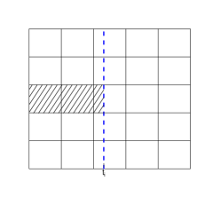
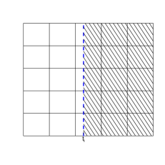
Given and censored data, simulate the “full data”. This is tractable since the censoring scheme tells us in which collection of bins the actual observation can be located. Then one can renormalise the density restricted to these bins and select a specific bin accordingly and generate the “full data”. Cf. Figure 1 for the two types of observations.
-
2.
Given the “full data”, draw samples for from the posterior which is of Dirichlet type.
5.2 Logistic Normal Graph Laplacian prior (LNGL-prior)
For the LNGL prior, one could opt for a data-augmentation scheme as well, but its attractiveness is lost since step (2) above is no longer of simple form. Therefore, we propose to bypass data-augmentation in this case. In an initial version of this paper we have proposed to use the probabilistic programming language Turing (see \citeNPGeXuGha) that is based on the Julia language (see \citeNPBezanson). With modest programming efforts, samples from the posterior can then be obtained by Hamiltonian Monte Carlo methods. For completeness, we present the core of such code in Appendix B. As can be seen, this contains about 10 lines of code and reads intuitively. However, a much faster algorithm can be derived by exploiting structure in the statistical model. The main idea is to use a non-centred parameterisation (\citeNPPapas) combined with a preconditioned Crank-Nicolson (pCN) scheme. The latter scheme dates back to \citeNPNeal98; a more recent exposition can be found in \citeNPCotter (see also \citeNPvdMSchauer in a different application setting).
Let denote the parameter vector (with all stacked). Let denote the “softmax”-function, defined by (this is a convenient choice, for our algorithm other mappings of a vector to a probability vector are also allowed). To sample from the prior of , with , we sample according to the following scheme
where with obtained from the Cholesky-decompostion of the graph-Laplacian matrix (with a small multiple of the identity matrix added): . Hence, we have introduced the random vector , which is centred in between and . The algorithm we propose is a Gibbs sampler which iteratively updates and . While our theoretical contribution assumes a prior on of Gamma type (see Assumption 3.3), the MCMC-algorithms in this section apply more generally to a prior distribution on that is supported on the positive halfline. Small values of induce more smoothing.
For updating conditional on we use the pCN scheme: pick a tuning parameters (typically chosen close to ) and propose a new value for by setting
| (14) |
where , independently of . Next, the Metropolis-Hastings (MH) acceptance rule is used to accept the proposal with probability , where denotes the likelihood, evaluated in (note that the prior ratio and proposal ratio cancel, as is symmetric in ). The likelihood can be simply and efficiently computed. To see this, consider Figure 1. Observations can be represented either by the left- or right figure. For the -th observation, we will denote by the vector that contains for each cell of the partition the fraction of the area that is shaded (so most values will be either or , only cells intersected by the blue dashed line will have entries in ). With this notation, it is easy to see that
To efficiently compute the loglikelihood, all that needs to be computed (once), is for each observation the vector of indices corresponding to the shaded boxes and the corresponding area fractions (this enables to exploit sparsity in when computing ). Also note that the Cholesky decomposition of only needs to be computed once.
For updating , conditional on the data and , we use a MH-step. We draw a proposal according to . It is accepted with probability
where denotes the prior density on and the term comes from the Jacobian. Note that a partial conjugacy for updating gets lost, even when employing a prior of inverseGamma type.
We conclude that in one iteration of the Gibbs-sampler, it is only required to do a simple MH-step for updating , sample as in (14) and use the MH-acceptance rule for this step as well.
5.1 Remark
In the prior specification we have postulated . Note that the prior on centers at zero. However, due to translation invariance of the softmax function, the same prior on is specified is we take , where is a vector that is a multiple of the vector with all elements equal to . Despite this identifiability issue, we have not encountered severe autocorrelation in traceplots for the LNGL-prior.
5.2 Remark
The same algorithm applies to more general censoring schemes. For example, suppose there are two checkup times, and the mark is only observed if the event took place in between those checkup times. This setting just corresponds to a different type of shading of boxes in Figure 1 but otherwise does not implicate any change to the numerical setting. Hence, the interval-censored continuous-mark model (see for instance \citeNPMW2008) is covered by our computational methods.
5.3 Numerical examples
In the following simulations, we compare the priors based on the Dirichlet distribution and the LNGL-prior. Updating can be done by incorporating a MH-step similar as for the LNGL-prior.
In each of the reported results, MCMC iterations were used, posterior means were computing after discarding the initial of the iterations as burnin. The algorithms were tuned such that the MH-steps have acceptance probability of about . For analysing a data set of size with bins, computing times are about seconds for iterations, using a Macbook-pro 2 GHz Quad-Core Intel Core i5 with 16 GB RAM. Note that the complexity of the algorithm scales with the number of bins and not with the sample size. From experiments with a large number of bins it appears that the acceptance rate for the pCN-step does not deteriorate, as also seen in other settings where pCN is utilised (Cf. [Cotter et al. (2013)]). Julia code (\citeNPBezanson) is available from https://github.com/fmeulen/CurrentStatusContinuousMarks. Computed Wasserstein distances are computed using the transport library in R.
Traceplots (not included here) confirm that in our experiments the chain on mixes well. Only in case of the D-prior, somewhat larger autocorrelation is observed in the chain for . The prior measure is taken to be the standard Exponential distribution for both priors.
We will consider the following data generated as independent replications of , where is drawn from the mixture experiment
with having density
In this case, it is easy to sample by first sampling from the marginal distribution of and then from the density of . In both cases the inverse of the cumulative distribution function can be computed in closed form. We assume that the censoring random vairable where is uniformly distributed on . This implies that the density of is given by . For the LNGL-prior we take where is defined in (4) and is the number of cells in the partition used to cover the support of the density.
5.3.1 Results for one dataset
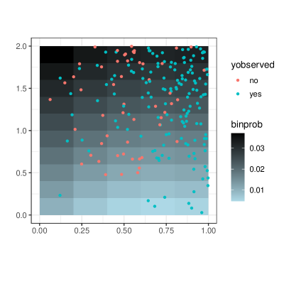
We sample observations from the model. The true density with observations superimposed is depicted in Figure 2. Horizontally/vertically we took bins, yielding equally sized bins. Note that the number of bins is way larger than the sample size; smoothing/penalisation being enforced by the prior.
In Figure 3 we compare the performance of the posterior mean estimator under both prior specifications.
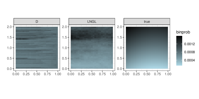
Smoothing induced by the LNGL-prior is quite apparent and the posterior mean estimate is visually more appealing. The latter is not surprising as the data-generating density is smooth.
5.3.2 Varying the number of bins
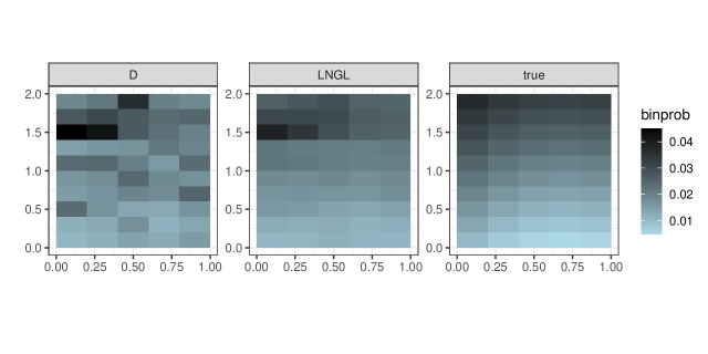
For each combination of prior/binning, we compute the Wasserstein distance (based on the /cityblock distance) between the probability vector of bin-masses of the estimate and the probability vector of bin masses of the true data-generating distribution. For a definition and motivation for using this distance we refer to Chapter 2.1 in \citeNPPanaretosZemel.
| prior/bins | |||
|---|---|---|---|
| D | |||
| LNGL |
Here “5/10” for example means: 5 bins in the horizontal direction 10 bins in the vertical direction. Especially with a large number of bins, the performance of the posterior mean using the D-prior is visually unappealing. Inspection of the traceplot for the parameter in this setting reveals large uncertainty. The LNGL-prior on the other hand seems quite robust in performance, once a sufficiently large number of bins is chosen.
5.3.3 Monte-Carlo study
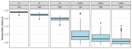
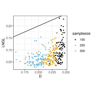
To compare the performance of the posterior mean estimator under both prior specifications we conduct a Monte-Carlo study. In each simulation run we
-
•
simulate a dataset;
-
•
compute the posterior mean under both the D- and LNGL-prior;
-
•
compute the Wasserstein distance (based on the /cityblock distance) between the probability vector of bin-masses of the estimate and the probability vector of bin masses of the true data-generating distribution.
We considered samples sizes and took the Monte-Carlo sample size equal to . In figures 6 and 7 we give two visualisations of the results. As expected, with large sample size the distance tends to be smaller. Additionally, the LNGL-prior appears to outperform the D-prior for this choice of data-generating distribution.
6 Discussion
The main theoretical contribution of this paper is Theorem 3.4. We expect the the rate in this theorem to be suboptimal. We conjecture to be the optimal rate, suggesting that Lemma 3.5 is sufficiently sharp. However, due to the tests constructed in Lemma 3.5 we obtain rate in our main result. We postpone further investigations to future research, where we also hope to obtain rates in global metrics.
The derived rate is non-adaptive. Adaptation can be achieved by employing a prior on the number of bins, see Chapter 10 in \citeNPGhoVaart. Computationally, such an approach is less attractive, as it requires a sampler on the larger space of the union of partitions. Instead, in our numerical work we have chosen to start off from a larger number of small bins, and have a prior on the scaling parameter take care of the regularisation. This yields an easily implementable and efficient computational scheme.
Appendix A Technical proofs
A.1 Lemma
Let and be bivariate density functions on . Assume the density of the censoring time, , is bounded. Then there exists a constant , independent of and such that
Proof.
Say is bounded by . If , then
This implies
| (15) |
∎
A.2 Lemma
Proof.
The proof is based on Lemma B.2 in \citeNPGhoVaart, which gives the following inequalities
| (16) |
Therefore, for we bound and . Substituting these bounds in (16) finishes the proof.
Step 1: showing that . By the definition of in (9), for any ,
By assumption (5) on , we have
Hence
| (17) |
Applying Lemma A.1 with and gives
where we used (17) to bound the first term on the right-hand-side. Using the inequality , we then have
| (18) |
Step 2. showing that for sufficiently large there exists a constant such that .
First note that
| (19) |
By Assumption 3.1, there exists such that for . Since we have . By Equation (17), there exists a (depending on and ) such that
Therefore
For sufficiently large we will have and therefore the denominator of the right-hand-side can be lower bounded by . This implies boundedness of for sufficiently large.
∎
Appendix B Programming details in the Turing language
For each observation, indexed by , we compute the vector of indices corresponding to the shaded area in Figure 1, as well as the fraction of the area that is shaded. This means that there is an -dimensional vector ci, where each element is of type (CensoringInformation). The structure CensoringInformation has two fields: ind and fracarea, holding indices and areafractions respectively. If L is the graph-Laplacian (with a small multiple of the identity matrix added), the model is specified as follows:
Here the loglikelihood is calculated using
References
- [Aitchison and Shen (1980)] Aitchison, J. and Shen, S.M. (1980) Logistic-normal distributions:Some properties and uses, Biometrika 67(2), p. 261–3444. https://doi.org/10.1093/biomet/67.2.261
- [Betancourt (2018)] Betancourt, M. (2018). A conceptual introduction to Hamiltonian Monte Carlo. arXiv:1701.02434.
- [Bezanson et al. (2017)] Bezanson, J., Edelman, A., Karpinski, S. and Shah, V. B. (2017). Julia: A Fresh Approach to Numerical Computing. Society for Industrial and Applied Mathematics. 59, p. 65–-98.
- [Chen et al. (2013)] Chen, D., Sun, J. and Peace, K. E. (2013). Interval-Censored Time-to-Event Data: Methods and Applications. Chapman and Hall/CRC Biostatistics Series.
- [Choudhuri et al. (2007)] Choudhuri, N., and Ghosal, S. and Roy, A. (2007). Nonparametric binary regression using a Gaussian process prior. Statistical Methodology. 4, p. 227–243.
- [Cotter et al. (2013)] Cotter, S., Roberts, G., Stuart, A. and White, D. (2013). MCMC Methods for Functions: Modifying Old Algorithms to Make Them Faster. Statistical Science, 28(3), p. 424-446.
- [Gao and Pavel (2018)] Gao, B. and Pavel, L. (2018) On the Properties of the Softmax Function with Application in Game Theory and Reinforcement Learning, arXiv:1704.00805
- [Ge, Xu & Ghahramani (2018)] Ge, H., Xu, K., and Ghahramani, Z. (2018). Turing: A Language for Flexible Probabilistic Inference. Proceedings of the Twenty-First International Conference on Artificial Intelligence and Statistics, PMLR: 84, p. 1682–-1690.
- [Ghosal, Ghosh & Van der Vaart (2000)] Ghosal, S., Ghosh, J.K. and Van der Vaart, A.W. (2000). Convergence rates of posterior distributions. Ann. Statist. 28, p. 500–531.
- [Ghosal & Van der Vaart (2007)] Ghosal, S., van der Vaart, A. (2007). Posterior convergence rates of Dirichlet mixtures at smooth densities. Ann. Statist. 2, p. 697–723.
- [Ghosal & Van der Vaart (2017)] Ghosal, S. and Van der Vaart, A.W. (2017). Fundamentals of Nonparametric Bayesian Inference. Cambridge University Press.
- [Groeneboom, Jongbloed & Witte (2011)] Groeneboom, P., Jongbloed, G. and Witte, B. I. (2011). Smooth Plug-in Inverse Estimators in the Current Status Mark Model. Scandinavian Journal of Statistics. 39, p. 15–33.
- [Groeneboom, Jongbloed & Witte (2012)] Groeneboom, P., Jongbloed, G. and Witte, B. I. (2012). A maximum smoothed likelihood estimator in thecurrent status continuous mark model. J. Nonparametr. Stat. 24, p. 85–101.
- [Groeneboom, Maathuis & Wellner (2008)] Groeneboom, P., Maathuis, M. H. and Wellner, J. A. (2008). Current status data with competing risks: Consistency and rates of convergence of the MLE. Ann. Statist. 36, p. 1031–1063.
- [Gugushvili et al. (2019)] Gugushvili, S., van der Meulen, F. H., Schauer, M. R. and Spreij, P. (2019). Nonparametric Bayesian volatility estimation. (eds) 2017 MATRIX Annals, MATRIX Book Series. 2, p. 279–302.
- [Gugushvili et al. (2018)] Gugushvili, S., van der Meulen, F. H., Schauer, M. R. and Spreij, P. (2018). Bayesian wavelet de-noising with the Caravan prior. arXiv:1810.07668, to appear in ESAIM.
- [Hartog & van Zanten (2017)] Hartog J. and van Zanten, H. (2017). Nonparametric Bayesian label prediction on a graph. arXiv:1612.01930
- [Hjort (1994)] Hjort, N.L. (1994) Bayesian Approaches to Non- and Semiparametric Density Estimation. In Bayesian Statistics 5. Proceedings of the Fifth Valencia International Meeting, June 5-9, 1994, edited by J. M. Bernardo, J. O. Berger, A. P. Dawid, and A. F. M. Smith,
- [Hoffman & Gelman (2014)] Hoffman, M. D. and Gelman, A. (2014). The No-U-turn Sampler: Adaptively Setting Path Lengths in Hamiltonian Monte Carlo. J. Mach. Learn. Res. 15, p. 1593–1623.
- [Huang & Louis (1998)] Huang, Y. and Louis, T. A. (1998). Nonparametric estimation of the joint distribution of survival time and mark variables. Biometrika. 85, p. 7856–-7984.
- [Hudgens, Maathuis & Gilbert (2007)] Hudgens, M. G., Maathuis, M. H. and Gilbert, P. B. (2007). Nonparametric estimation of the joint distribution of a survival time subject to interval censoring and a continuous mark variable. Biometrics 63, p. 372–-380.
- [Maathuis & Wellner (2008)] Maathuis, M. H. and Wellner, J. A. (2008). Inconsistency of the MLE for the joint distribution of interval-censored survival times and continuous marks. Scand. J. Statist. 35, p. 83–-103.
- [Lenk (1988)] Lenk, P.J. (1988). The logistic normal distribution for Bayesian, non-parametric, predictive densities .J. Amer. Statist. Assoc.83(402), p. 509–516, MR0971380.
- [Van der Meulen & Schauer (2017)] Van der Meulen, F.H. and Schauer, M. (2017) Bayesian estimation of discretely observed multi-dimensional diffusion processes using guided proposals. Electron. J. Statist. 11(1), p. 2358–2396. doi:10.1214/17-EJS1290, https://projecteuclid.org/euclid.ejs/1495850628
- [Moala and O’Hagan (2010)] Moala, F. A. and O’Hagan, A. (2010). Elicitation of multivariate prior distributions: A nonparametric Bayesian approach. Journal of Statistical Planning and Inference. 140, p. 1635–3758.
- [Murphy (2013)] Murphy, K. Machine Learning: a Probabilistic Perspective. MIT Press.
- [Neal (1998)] Neal, R. M.(1998). Regression and classifica-tion using Gaussian process priors. Available at http://www.cs.toronto.edu/~radford/valencia.abstract.html
- [Panaretos and Zemel (2020)] Panaretos, V. and Zemel, Y. (2020) An Invitation to Statistics in Wasserstein Space, Springer.
- [Papaspiliopoulos et al. (2003)] Papaspiliopoulos, O. Roberts, G.O. and Sköld, M. Non-centered parame-terizations for hierarchical models and data augmentation (with discussion), in BayesianStatistics 7 (Tenerife 2002), p. 307–326. Oxford Univ. Press, New York.MR2003180
- [Robert et al. (2018)] Robert C. P., Elvira V., Tawn N., and Wu C. (2018). Accelerating MCMC algorithms Wiley Interdiscip. Rev. Comput. Stat. 10, e1435.
- [Ting et al. (2010)] Ting, D., Huang, L. and Jordan, M.I. (2010) An Analysis of the Convergence of Graph Laplacians, In Proceedings of the 27th International Conference on Machine Learning (ICML), Haifa, Israel, 2010.
- [van de Meent et al. (2018)] van de Meent, J. W., Paige, B., Yang, H. and Wood, F. (2018). An Introduction to Probabilistic Programming. arXiv:1809.10756.
- [Van der Vaart (1998)] Van der Vaart, A.W. (1998). Asymptotic Statistics. Cambridge University Press.
- [Van der Vaart and Van Zanten (2007)] Van der Vaart, A.W. and Van Zanten, J.H. (2007) Bayesian inference with rescaledGaussian process priors, Electronic Journal of Statistics 1, p. 433-448.