Parallelising MCMC via Random Forests

Abstract

For Bayesian computation in big data contexts, the divide-and-conquer MCMC concept splits the whole data set into batches, runs MCMC algorithms separately over each batch to produce samples of parameters, and combines them to produce an approximation of the target distribution. In this article, we embed random forests into this framework and use each subposterior/partial-posterior as a proposal distribution to implement importance sampling. Unlike the existing divide-and-conquer MCMC, our methods are based on scaled subposteriors, whose scale factors are not necessarily restricted to $1$ or to the number of subsets. Through several experiments, we show that our methods work well with models ranging from Gaussian cases to strongly non-Gaussian cases, and include model misspecification.

1 Introduction

Markov chain Monte Carlo (MCMC) algorithm, a generic sampling method, is ubiquitous in modern statistics, especially in Bayesian fields. MCMC algorithms require only the evaluation of the target pointwise, up to a multiple constant, in order to sample from it. In Bayesian analysis, the object of main interest is the posterior, which is not in closed form in general, and MCMC has become a standard tool in this domain. However, MCMC is difficult to scale and its applications are limited when the observation size is very large, for it needs to sweep over the entire observations set in order to evaluate the likelihood function at each iteration. Recently, many methods have been proposed to better scale MCMC algorithms for big data sets and these can be roughly classified into two groups Bardenet et al. (2017): divide-and-conquer methods and subsampling-based methods.

For divide-and-conquer methods, one splits the whole data set into subsets, runs MCMC over each subset to generate samples of parameters and combine these to produce an approximation of the true posterior. Depending on how MCMC is handled over the subsets, these methods can be further classified into two sub-categories. Let $\mathcal{X}$ be the whole data set and $\mathcal{X}_{1},\cdots,\mathcal{X}_{K}$ be the subsets. Denote $\pi_{0}$ by the prior distribution over the parameter $\theta$. One approach (Neiswanger et al., 2014, Nemeth and Sherlock, 2018, Scott et al., 2016, Wang and Dunson, 2013, Wang et al., 2015) consists in running MCMC over

$$\pi_{k}(\theta|\mathcal{X}_{k})\propto\left(\pi_{0}(\theta)\right)^{1/K}\prod_{x\in\mathcal{X}_{k}}p(x|\theta).$$

The other approach (Minsker et al., 2014, Srivastava et al., 2015) targets

$$\pi_{k}(\theta|\mathcal{X}_{k})\propto\pi_{0}(\theta)\prod_{x\in\mathcal{X}_{k}}p(x|\theta)^{K}.$$

For subsampling-based methods, one uses a partition of the whole data set to estimate the MH acceptance ratio at each iteration in order to accelerate the MCMC algorithms. These approaches can also be classified into two finer classes: exact subsampling methods and approximate subsampling methods, according to their outputs. Exact subsampling approaches typically require to explore an augmented space and to treat the target distribution as its invariant marginal distribution. One direction (Quiroz et al., 2016) is to take advantage of pseudo-marginal MCMC (Andrieu and Roberts, 2009) via constructing unbiased estimators of point-wise evaluations of the target density with subsets of the data. Another approach is to leverage the piecewise deterministic Markov processes (Bierkens et al., 2018, Bierkens et al., 2019, Bouchard-Côté et al., 2018, Davis, 1984, Davis, 1993, Fearnhead et al., 2018, Sherlock and Thiery, 2017, Vanetti et al., 2017), which take the targets as the marginal distributions of their invariant distributions. Approximate subsampling approaches aim at constructing an approximation of the target distributions. One approach (Bardenet et al., 2014, 2017) is to determine the acceptance of the proposals with high probability using subsets of the data. Another approach (Chen et al., 2014; Ding et al., 2014; Welling and Teh, 2011), is based on direct modifications of exact methods. The seminal work in this direction is stochastic gradient Langevin dynamics (SGLD) (Welling and Teh, 2011).

In this article, we propose two methods to scale MCMC algorithms, which are based on divide-and-conquer principles. However, unlike the former divide-and-conquer approaches, we run MCMC over

$$\pi_{k}(\theta|\mathcal{X}_{k})\propto\left\{\left(\pi_{0}(\theta)\right)^{1/K}\prod_{x\in\mathcal{X}_{k}}p(x|\theta)\right\}^{\lambda},$$

where $\lambda$ is not necessarily restricted to $1$ or $K$. Further, we use random forests (Breiman, 2001) to learn approximations of the subposteriors and we take advantage of them to approximate the true posterior by an additional MCMC or importance sampling step. Section 2 describes the proposed methods in details and several numerical examples are presented in section 3. In section 4, we discuss the limitations of these methods and conclude the paper.

2 Methodology

Denote by $\mathcal{X}=\left\{x_{1},x_{2},\cdots,x_{N}\right\}$ the whole data set of observations, where $x_{i}\sim p_{\theta}(\cdot)$ i.i.d. and $\theta\in\Theta\subset\mathbb{R}^{d}$. Let $\pi_{0}(\theta)$ denote the prior distribution on the parameter space $\Theta$. Splitting the whole data set $\mathcal{X}$ into subsets $\mathcal{X}_{1},\cdots,\mathcal{X}_{K}$, each with same size $m=\frac{N}{K}$, the target of interest is the posterior distribution:

$$\pi(\theta|\mathcal{X})\propto\pi_{0}(\theta)\prod_{i=1}^{N}p(x_{i}|\theta)$$

For each subset $\mathcal{X}_{k}$, $k=1,\cdots,K$, we define the $\lambda_{k}$-subposterior as:

$$\pi_{k}^{\lambda_{k}}(\theta|\mathcal{X}_{k})=\frac{\left(\gamma_{k}(\theta|\mathcal{X}_{k})\right)^{\lambda_{k}}}{Z_{k,\lambda_{k}}},\quad\gamma_{k}(\theta|\mathcal{X}_{k})=\pi_{0}(\theta)^{\frac{1}{K}}\prod_{x\in\mathcal{X}_{k}}p(x|\theta),$$

where $Z_{k,\lambda_{k}}$ is the normalising constant of $\left(\gamma_{k}(\theta|\mathcal{X}_{k})\right)^{\lambda_{k}}$.

In the divide-and-conquer paradigm, one applies MCMC algorithms on each subposterior, generates samples from them and combines these samples to approximate the true posterior distribution. Existing divide-and-conquer MCMC methods treat these $\lambda_{k}$’s in two possible ways: one is to set $\lambda_{k}=1$ for all $k=1,\cdots,K$, in e.g. consensus Monte Carlo and Weierstrass sampler; the other is to set $\lambda_{k}=K$, in e.g. WASP (Srivastava et al., 2015), M-posterior (Minsker et al., 2014). By contrasat, in our method, the choice of $\lambda_{k}$ is not restricted to these two options. Besides, the above mentioned methods, except for the one proposed by Nemeth and Sherlock (2018), ignore a valuable byproduct — namely the value of the target distribution at the proposed sample points — of an MCMC algorithm. However, when compared with Nemeth and Sherlock (2018), our methods differ in two aspects: one is to use the scaled subposterior, the other is that the learning algorithm is cheaper at both training and prediction stages.

In our method, we embed a regression procedure into a divide-and-conquer perspective in order to propose approximations of the subposterior density functions and use them to produce an approximation of the true posterior. Specifically, we run MCMC algorithms with MH steps, such as MCMC, HMC, MALA, over $\pi_{k}^{\lambda_{k}}(\theta|\mathcal{X}_{k})$ to obtain samples $\{\theta_{1}^{k},\theta_{2}^{k},\cdots,\theta_{T}^{k}\}$. Considering the construction of MH acceptance ratios, we just need to evaluate $\log{\gamma_{k}(\theta|\mathcal{X}_{k})}$ pointwise, instead of computing the harder target, $\pi_{k}^{\lambda_{k}}(\theta|\mathcal{X}_{k})$, in order to bypass the derivation of the normalising constant, a common numerical problem in computation. As a byproduct, we can get the evaluations of $\log{\gamma_{k}(\theta|\mathcal{X}_{k})}$ at certain points $\{\vartheta_{1}^{k},\vartheta_{1}^{k},\cdots,\vartheta_{T_{k}}^{k}\}$, which are the proposed values in MCMC algorithms. Running random forests or other regression machine learning algorithms on

$$\left\{\bigg{(}\vartheta_{1}^{k},\log\gamma_{k}(\vartheta_{1}^{k}|\mathcal{X}_{k})\bigg{)},\bigg{(}\vartheta_{2}^{k},\log\gamma_{k}(\vartheta_{2}^{k}|\mathcal{X}_{k})\bigg{)},\cdots,\left(\vartheta_{T_{k}}^{k},\log\gamma_{k}(\vartheta_{T_{k}}^{k}|\mathcal{X}_{k})\right)\right\}$$

provides an estimator, $f_{k}$, of $\log\{\gamma_{k}(\theta|\mathcal{X}_{k})\}$. The uses of such $f_{k}$’s, $k=1,\cdots,K$, are double: one is to approximate $\pi(\theta|\mathcal{X})$ with

$$f(\theta)=\displaystyle{\exp\left\{\sum_{k=1}^{K}f_{k}(\theta)\right\}}$$

and to run an additional MCMC over $f$ to obtain samples which are regarded as an approximation of the posterior distribution; the other usage is to approximate $\pi(\theta|\mathcal{X})$ with $f(\theta)$ and apply importance sampling algorithm on $f$ with proposal distribution $\gamma_{k}^{\lambda_{k}}(\theta|\mathcal{X}_{k})$.

Remark 1: (Scale factors) The scale factor $\lambda_{k}$ is used to control the uncertainty in the subposterior. Roughly speaking, it controls the range of the region from which the embedded regression algorithm learns each subposterior. When the scale factor is too large, for instance, when $\lambda_{k}=100K,k=1,\cdots,K$, each scaled subposterior has small uncertainty, which may lead to the resulting MCMC samples not overlapping with one another. In the event this happens, the approximation $f_{k}$ cannot provide useful information on the region where $\gamma_{j}(\theta|\mathcal{X}_{j})$ is high for $j\neq k$ and neither of the additional MCMC method and IS correction works. On the other hand, if the scale factor is too small, for example when $\lambda_{k}=0.001,k=1,\cdots,K$, we need more pairs of sample points and corresponding logarithms of the probability density function (pdf) of each subposterior to train a good approximation, even though the subposteriors are more likely to overlap. In some cases where we can easily and cheaply obtain approximations of the means and covariances of the true posterior and subposteriors (here, $\lambda_{k}=1,k=1,\cdots,K$), we can choose $\lambda_{k}$ such that a chosen high probability posterior region is covered by one such region for the subposterior $\pi_{k}$. Specifically, in a one-dimension case ($d=1$), let $\hat{\theta}$, $\hat{\theta}_{k}$, $\hat{\sigma}$ and $\hat{\sigma}_{k}$ be the approximations of the means and standard deviations of the true posterior and the subposterior $\pi_{k}$, respectively. Denote $\delta_{k}=\max\{|\hat{\theta}_{k}-\hat{\theta}-2\hat{\sigma}|,|\hat{\theta}_{k}-\hat{\theta}+2\hat{\sigma}|\}$ and choose $\lambda_{k}=(\delta_{k}/\hat{\sigma}_{k})^{-2}$. By Markov’s inequality, $\pi_{k}^{\lambda_{k}}$ covers most of a high probability region for the true posterior. In high dimension cases, i.e., when $d>1$, we can choose the scale factors as the minimal ones according to each marginal component.

Remark 2: (Regression algorithms) Considering the easy implementation, strong learning ability of non-linearity and robustness of random forests, we apply this modelling technique to learn cheapapproximations of the subposterior density function. Of course, other regression algorithms could be chosen instead. However, when compared with random forests, these other machine learning algorithms, such as support vector machines or neural networks, have a higher cost in terms of hyper-parameters to set, while random forests are both easy to tune and relatively robust. Besides, prediction by random forests is scalable, that is, given the training set size $M$, the cost of predicting the output of a new input is just $\mathcal{O}(\log(M))$. When we use these approximations of the subposteriors $f_{k}$ to run an additional MCMC, the evaluation cost of a new proposal is of order $\mathcal{O}(K\log(M))$, to compare with $\mathcal{O}(KM)$ in memory-based algorithms, such as local linear/polynomial regression, nonparametric kernel density estimation, Gaussian processes.

Remark 3: (Combination of Importance Sampling) For our second method, we use importance sampling over each subposterior and combine them to approximate the true posterior, without need to run an additional MCMC. However, considering that the subposteriors are more spread out than the true posterior, a large portion of their samples has extremely low weights and need be discarded to achieve an better approximation of the true posterior. Besides, in importance sampling, the proposal samples are independent. As a result, in the MCMC stage of subposteriors, we thin out the accepted samples such that they are approximately independent. More precisely, suppose $\left\{\theta_{1}^{k},\cdots,\theta_{T}^{k}\right\}$ are the well tuned samples of $\pi_{k}^{\lambda_{k}}$, their weights are

$$w_{t}^{k}\propto\exp\left\{\sum_{j=1}^{K}f_{j}(\theta_{t}^{k})-\lambda_{k}f_{k}(\theta_{t}^{k})\right\},$$

for $t=1,\cdots,T$. Let $\sigma$ be a permutation of $\{1,\cdots,T\}$ such that $w_{\sigma(1)}^{k}\geq w_{\sigma(2)}^{k}\geq\cdots\geq w_{\sigma(T)}^{k}$. According to a pre-specified truncation probability $p$, we choose $i_{k}=\min\{i\mathrel{\mathop{\ordinarycolon}}\sum_{\ell=1}^{i}w^{k}_{\sigma(\ell)}\geq p\}$ and treat $\tilde{\pi}_{k}=\sum_{\ell=1}^{i_{k}}\tilde{w}_{\ell}^{k}\delta_{\theta_{\sigma{\ell}}^{k}}$, where $\tilde{w}_{\ell}^{k}={w_{\ell}^{k}}\big{/}{\sum_{r=1}^{i_{k}}w_{r}^{k}}$. Generally, we can choose $p=0.99,0.999,0.9999.$ Considering that the $i_{k}$’s are unequal across $k=1,\cdots,K$ by stochasticity, some $\tilde{\pi}_{k}$’s have more atoms than average, while others have fewer atoms. We weight the approximation $\tilde{\pi}_{k}$ proportional to their effective sample sizes (ESS) (Liu, 2008), that is, we approximate the true posterior with

$$\hat{\pi}\propto\sum_{k=1}^{K}ESS_{k}\tilde{\pi}_{k},\quad ESS_{k}=\frac{i_{k}}{1+\mathbb{V}_{k}}$$

where $\mathbb{V}_{k}$ is the variance of $\{i_{k}w_{\sigma(1)}^{k},\cdots,i_{k}w_{\sigma(i_{k})}^{k}\}$.

Remark 4: (Computation complexity)

1. In the divide-and-conquer stage, the computation cost is $\mathcal{O}(T_{k}N/K)$ on each computation node and we generate $T$ well-turned samples points.

2. In the regression training stage, the cost for each random forest is $\mathcal{O}(T_{k}\log T_{k})$

3. In the combination stage

   1. To run an additional MCMC, the computation cost of a proposal point is $\mathcal{O}(K\log T_{k})$.

   2. To run importance sampling, the cost of weighting all well-tuned samples of all subposteriors on each computation node is $\mathcal{O}(KT\log T_{k})$.

3 Numerical Experiments

For simplicity of notations, we call the first method RF-MH and the second one RF-IS. In this section, we apply our methods to several examples, from Gaussian posterior to strongly non-Gaussian posteriors and to model misspecification case. We compare our methods with consensus Monte Carlo (CMC) Scott et al. (2016), nonparametric KDE (Nonpara) Neiswanger et al. (2014) and Weierstrass sampler (Weierstrass) Wang and Dunson (2013).

3.1 Bimodal Posterior

In this example, the parameter $\theta=(\theta_{1},\theta_{2})$ drives the model

$$\begin{split}X\sim\frac{1}{2}\mathcal{N}(\theta_{1},2)+\frac{1}{2}\mathcal{N}(\theta_{1}+\theta_{2},2),\end{split}$$

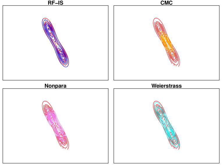
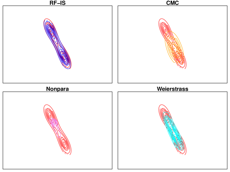
This toy example comes from Welling and Teh (2011). We use the flat prior $\pi_{0}(\theta_{1},\theta_{2})\propto 1$. We draw $n=200$ observations $\{X_{1},X_{2},\cdots,X_{200}\}$ from the model with $\theta_{1}=0,\theta_{2}=1$. In order to apply the parallel MCMC algorithms, we set $K=10$ and $20$. There are two configurations of the parameters corresponding to the observations, $(\theta_{1},\theta_{2})=(0,1)$ and $(1,-1)$. When the observation size is moderate, both configurations can be detected and the posterior is bimodal. While the size is too large, Markov chain will be stuck at one mode, which will output a unimodal posterior. In order to show that our proposed methods can handle non-Gaussian posterior distributions, we set a moderate $n=200$. We generate 500,000 samples for each subposterior, discard the first 100,000 points and thin out the rest per 100 sample points. In this example, we set $\lambda_{k}=1,k=1,\cdots,K$ and train each random forest with $10$ random partition trees on a random subset of those sample sets with size 50,000. In Figure $1$, we compare the contours of the resulting pdfs derived from the samples for each method for $K=10$. It is clear that consensus Monte Carlo could not capture the bimodal feature of the posterior, and nonparametric KDE gives unequal weights for two modes, while our methods and Weierstrass sampler perform very well. In Figure $2$, we set $K=20$, except for our method, other methods deviate the true posteriors. In Table 1, we compare the time budget of each method. In this example, the MCMC stage dominates in the computation cost, all but the nonparametric KDE have the same order of time budget. Since KDE is memory-based, its prediction cost is $\mathcal{O}(T^{2})$, while our method exhibits scalable prediction cost.

Figure 1: Example 1: Comparisons of the contours of true posterior (red), RF-IS(blue), consensus Monte Carlo (orange), KDE (violet) and Weierstrass sampler (cyan) for $K=10$

Figure 2: Example 1: Comparisons of the contours of true posterior (red), RF-IS(blue), consensus Monte Carlo (orange), KDE (violet) and Weierstrass sampler (cyan) for $K=20$

K	RF-IS	CMC	Nonpara	Weierstrass
$K=10$	MCMC   $54.8$	MCMC   $54.8$	MCMC   $54.8$	MCMC   $54.8$
	Training   $2.8$
	Weighting  $0.3$	Combination   $0.1$	Combination   $109.3$	Combination   $0.8$
	Total   $57.9$	Total   $54.9$	Total   $164.1$	Total   $55.6$
$K=20$	MCMC   $52.8$	MCMC   $52.8$	MCMC   $52.8$	MCMC   $52.8$
	Training   $2.8$
	Weighting   $0.6$	Combination   $0.2$	Combination   $403.2$	Combination   $1.6$
	Total   $56.2$	Total   $53.0$	Total   $456.0$	Total   $54.4$

Table 1: Time budget of Example 1 (in seconds).

3.2 Moon-shaped Posterior

This is a toy example which is unidentifiable in the parameters. Denote $\boldsymbol{\theta}=(\theta_{1},\theta_{2})\in[0,\infty)^{2}$ as parameters, the observations, $X_{1},\cdots,X_{N}$, given the parameter $\boldsymbol{\theta}$, are generated from

$$X\sim\mathcal{N}(\sqrt{\theta_{1}}+\sqrt{\theta_{2}},2),\quad\theta_{1}\geq 0,\theta_{2}\geq 0$$

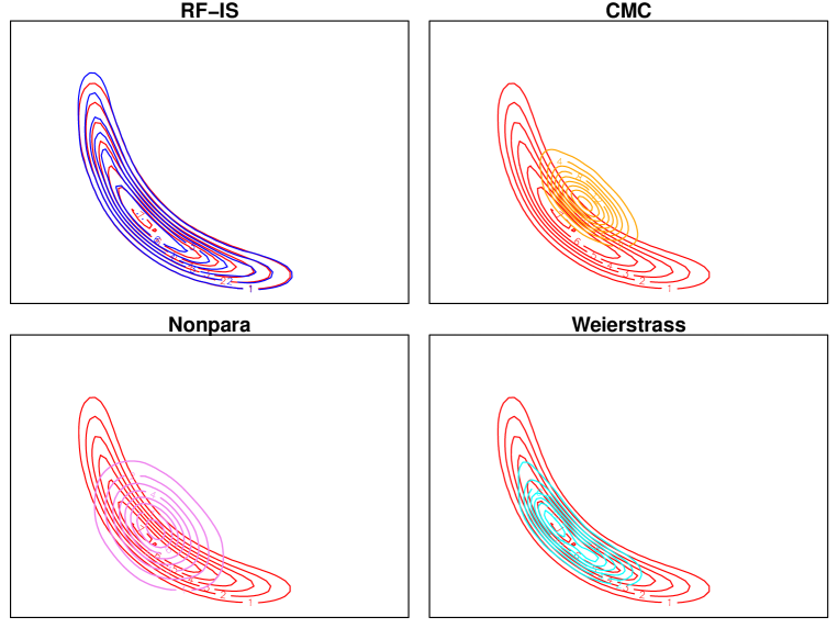
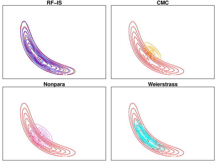
In this model, in light of the non-identifiability, the posterior is moon-shaped and strongly non-Gaussian. In our experiment, we generate observations from standard normal distribution, $\mathcal{N}(0,1)$, set $N=1000,K=10,20,\lambda_{k}=1,k=1,\cdots,K$ and draw 500,000 sample points from each subposterior, burn the first 100,000 ones and thin out the rest per 100 points. Using large proposal points of each subposterior, we train each random forest with $10$ random partition trees on random subset of the samples set with size 50,000. Figure $3$ compares the performances of each method for $K=10$ case. In this strongly non-Gaussian case, consensus Monte Carlo and nonparametric KDE produce Gaussian posteriors. To some extent the Weierstrass sampler is able to learn this non-Gaussian posterior, but our method has the best performance thanks to its random forest construct. In Figure 4, $K=20$ and we can check that the Weierstrass sampler becomes worse while our method still approximates closely the target. In Table 2, we present the time budget of each method. We can see there that nonparametric KDE is the most costly solution, since it is memory-based and its cost of a new prediction is $\mathcal{O}(T^{2})$. Since the MCMC stage over subsets dominates the computing budget, our methods has the same order of time budget as consensus Monte Carlo and Weierstrass samplers.

Figure 3: Example 2: Comparisons of the contours of true posterior (red), RF-IS(blue), consensus Monte Carlo (orange), KDE (violet) and Weierstrass sampler (cyan) for $K=10$

Figure 4: Example 2: Comparisons of the contours of true posterior (red), RF-IS(blue), consensus Monte Carlo (orange), KDE (violet) and Weierstrass sampler (cyan) for $K=20$

K	RF-IS	CMC	Nonpara	Weierstrass
$K=10$	MCMC   $67.6$	MCMC   $67.6$	MCMC   $67.6$	MCMC   $67.6$
	Training   $2.8$
	Weighting  $0.3$	Combination   $0.1$	Combination   $101.7$	Combination   $0.7$
	Total   $70.7$	Total   $67.7$	Total   $169.3$	Total   $68.3$
$K=20$	MCMC   $58.7$	MCMC   $58.7$	MCMC   $58.7$	MCMC   $58.7$
	Training   $2.7$
	Weighting   $0.7$	Combination   $0.2$	Combination   $371.5$	Combination   $1.5$
	Total   $62.1$	Total   $58.9$	Total   $430.2$	Total   $60.2$

Table 2: Time budget of Example 2 (in seconds).

3.3 Misspecification Example

This example is borrowed from Bardenet et al. (2017) and is to show that with a suitable selection of the scale factors, $\lambda_{k}$, our methods are robust to misspecification of models. In the example, the model is

$$X\sim\mathcal{N}(\mu,\sigma^{2}),$$

the parameter is $\boldsymbol{\theta}=(\mu,\sigma^{2})$. In the experiments, we generate two data sets, each having $N=10000$ points $X_{1},\cdots,X_{10000}$, from log-normal distribution, $\mathcal{LN}(0,1)$ and standard normal distribution, $\mathcal{N}(0,1)$, respectively, and choose the flat prior, $p(\mu,\sigma^{2})\propto 1$. Let $K=10$ and choosing $\lambda_{k}$ from the method in Remark 1. In more details, by the maximum likelihood estimator, we have, over the whole data set,

$$\hat{\boldsymbol{\theta}}=\left({\sum_{i=1}^{N}x_{i}}\big{/}{N},{\sum_{i=1}^{N}(x_{i}-\bar{x})^{2}}\big{/}{N}\right)\qquad\qquad\hat{\boldsymbol{\sigma}}_{\boldsymbol{\theta}}=\left(\sqrt{{\hat{\theta}_{2}}\big{/}{N}},\sqrt{{2\hat{\theta}_{2}^{2}}\big{/}{N}}\right)$$

For each subset $\mathcal{X}_{k}$, we can obtain $\hat{\boldsymbol{\theta}}^{(k)}$ and $\hat{\boldsymbol{\sigma}}_{\boldsymbol{\theta}^{(k)}}$ similarly. Set

$$\lambda_{k,1}=\left(\frac{\max\{|\hat{\theta}^{(k)}_{1}-\hat{\theta}_{1}-2\hat{\sigma}_{\theta_{1}}|,|\hat{\theta}^{(k)}_{1}-\hat{\theta}_{1}+2\hat{\sigma}_{\theta_{1}}|\}}{\hat{\sigma}_{\theta^{(k)}_{1}}}\right)^{-2}$$

$$\lambda_{k,2}=\left(\frac{\max\{|\hat{\theta}^{(k)}_{2}-\hat{\theta}_{2}-2\hat{\sigma}_{\theta_{2}}|,|\hat{\theta}^{(k)}_{2}-\hat{\theta}_{2}+2\hat{\sigma}_{\theta_{2}}|\}}{\hat{\sigma}_{\theta^{(k)}_{2}}}\right)^{-2}$$

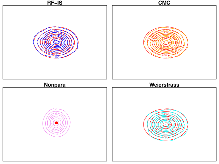
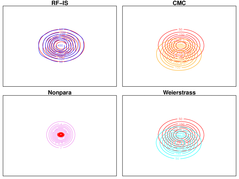
and $\lambda_{k}=\min\{\lambda_{k,1},\lambda_{k,2}\}$. We generate 500,000 sample points from each subposterior, discard the first 100,00 values and thin out the rest per 100 points for Gaussian case and per 10 points for Log-Normal case. Each random forest is trained with 10 random partition trees. Figure $5$ and Figure $6$ present the performance of each method under the normal distribution and log-normal distribution respectively. In each case, samples of nonparametric KDE are far away from the true posterior, as some subposteriors do not cover the high probability region of true posterior. In the normal case, RF-IS, consensus Monte Carlo and Weierstrass sampler all perform very well. However, only our method appears to be robust to model misspecification, the other ones deviating from the true posteriors to some extent in the log-normal case. In Table 3, we compare the time budget for each method and we can spot that the nonparametric KDE is the most costly in the log-normal case as the size of samples from each subposterior is quite large.

Figure 5: Example 3: For normal observations, comparisons of the contours of true posterior (red), RF-IS(blue), consensus Monte Carlo (orange), KDE (violet) and Weierstrass sampler (cyan).

Figure 6: Example 3: For log-normal observations, comparisons of the contours of true posterior (red), RF-IS(blue), consensus Monte Carlo (orange), KDE (violet) and Weierstrass sampler (cyan).

Model	RF-IS	CMC	Nonpara	Weierstrass
$\mathcal{N}(0,1)$	MCMC   $63.9$	MCMC   $65.2$	MCMC   $65.2$	MCMC   $65.2$
	Training   $117.4$
	Weighting  $1.1$	Combination   $0.1$	Combination   $99.6$	Combination   $0.8$
	Total   $182.4$	Total   $65.3$	Total   $164.8$	Total   $66.0$
$\mathcal{LN}(0,1)$	MCMC   $67.4$	MCMC   $69.2$	MCMC   $69.2$	MCMC   $69.2$
	Training   $119.4$
	Weighting   $5.3$	Combination   $0.9$	Combination   $1114.4$	Combination   $7.5$
	Total   $192.1$	Total   $70.1$	Total   $1183.6$	Total   $76.7$

Table 3: Time budget of Example 3 (in seconds).

4 Conclusion

Our proposal is therefore to combine divide-and-conquer MCMC methods, random forests and importance sampling to scale MCMC algorithms. Unlike the existing divide-and-conquer MCMC methods, we propose to scale the partial posterior with factors which are not necessarily $1$ or the selected number of subsets or to be equal with one another. Given suitable scale factors, we can achieve overlapping subposteriors, a feature that is of the highest importance in the combination stage. Considering its strong non-linear learning ability, an easy implementation and a scalable prediction cost, a method based on random forests embedded in a divide-and-conquer MCMC framework delivers cheap and robust approximations of the subposteriors. Overall, our numerical experiments achieve good performance, from Gaussian cases to strongly non-Gaussian cases, which are further to model misspecification, exhibiting to some extent limitations of existing divid-and-conquer scalable MCMC methods.

The main limitation of our method is the curse of dimensionality in random forest training. In high dimensional parameter spaces, it requires more sample points to train each random forest learner. The second shortcoming is the necessary selection of scale factors. We can offer no generic method to tune them, except in some cases where we can obtain cheap estimations of the means and covariances of the true posteriors and the subposteriors.

In fact, if we can roughly detect a high probability region, $E$, for the posterior, we can discard the stage of running MCMC over subsets, instead generating points from $E$ uniformly and training the random forests with these points and their corresponding pdf values for each subposterior, respectively. Besides, the result of our methods can also be used to produce such $E$. When considering the practical implementation of this extension, since RF-MH need store $K$ random forests at each iteration in order to predict the likelihood value, it proves more costly than RF-IS, even though the computation complexity is the same as RF-IS in theory.

References

- Andrieu and Roberts (2009) Andrieu, C. and Roberts, G. O. (2009). The pseudo-marginal approach for efficient Monte Carlo computations. The Annals of Statistics 697–725.
- Bardenet et al. (2014) Bardenet, R., Doucet, A. and Holmes, C. (2014). Towards scaling up Markov chain Monte Carlo: an adaptive subsampling approach. Proceedings of the 31st International Conference on Machine Learning (ICML-14) 405–413.
- Bardenet et al. (2017) Bardenet, R., Doucet, A. and Holmes, C. (2017). On Markov chain Monte Carlo methods for tall data. Journal of Machine Learning Research, 18 1–43.
- Bierkens et al. (2018) Bierkens, J., Bouchard-Côté, A., Doucet, A., Duncan, A. B., Fearnhead, P., Lienart, T., Roberts, G. and Vollmer, S. J. (2018). Piecewise deterministic Markov processes for scalable Monte Carlo on restricted domains. Statistics & Probability Letters, 136 148 – 154. The role of Statistics in the era of big data, URL http://www.sciencedirect.com/science/article/pii/S016771521830066X.
- Bierkens et al. (2019) Bierkens, J., Fearnhead, P. and Roberts, G. (2019). The zig-zag process and super-efficient sampling for Bayesian analysis of big data. The Annals of Statistics, 47 1288–1320. URL https://doi.org/10.1214/18-AOS1715.
- Bouchard-Côté et al. (2018) Bouchard-Côté, A., Vollmer, S. J. and Doucet, A. (2018). The bouncy particle sampler: A nonreversible rejection-free Markov chain Monte Carlo method. Journal of the American Statistical Association, 113 855–867.
- Breiman (2001) Breiman, L. (2001). Random forests. Machine learning, 45 5–32.
- Chen et al. (2014) Chen, T., Fox, E. and Guestrin, C. (2014). Stochastic gradient Hamiltonian Monte Carlo. Proceedings of the 31st International Conference on Machine Learning (ICML-14) 1683–1691.
- Davis (1984) Davis, M. H. (1984). Piecewise-deterministic Markov processes: A general class of non-diffusion stochastic models. Journal of the Royal Statistical Society. Series B (Methodological) 353–388.
- Davis (1993) Davis, M. H. (1993). Markov Models & Optimization, vol. 49. CRC Press.
- Ding et al. (2014) Ding, N., Fang, Y., Babbush, R., Chen, C., Skeel, R. D. and Neven, H. (2014). Bayesian sampling using stochastic gradient thermostats. Advances in Neural Information Processing Systems (NIPS 2014) 3203–3211.
- Fearnhead et al. (2018) Fearnhead, P., Bierkens, J., Pollock, M. and Roberts, G. O. (2018). Piecewise deterministic Markov processes for continuous-time Monte Carlo. Statistical Science, 33 386–412. URL https://doi.org/10.1214/18-STS648.
- Liu (2008) Liu, J. S. (2008). Monte Carlo strategies in scientific computing. Springer Science & Business Media.
- Minsker et al. (2014) Minsker, S., Srivastava, S., Lin, L. and Dunson, D. (2014). Scalable and robust Bayesian inference via the median posterior. Proceedings of the 31st International Conference on Machine Learning (ICML-14) 1656–1664.
- Neiswanger et al. (2014) Neiswanger, W., Wang, C. and Xing, E. (2014). Asymptotically exact, embarrassingly parallel MCMC. UAI’14 Proceedings of the Thirtieth Conference on Uncertainty in Artificial Intelligence 623–632. ArXiv preprint arXiv:1311.4780.
- Nemeth and Sherlock (2018) Nemeth, C. and Sherlock, C. (2018). Merging MCMC subposteriors through Gaussian-process approximations. Bayesian Analysis, 13 507–530. URL https://doi.org/10.1214/17-BA1063.
- Quiroz et al. (2016) Quiroz, M., Villani, M. and Kohn, R. (2016). Exact subsampling MCMC. arXiv preprint arXiv:1603.08232.
- Scott et al. (2016) Scott, S. L., Blocker, A. W., Bonassi, F. V., Chipman, H. A., George, E. I. and McCulloch, R. E. (2016). Bayes and big data: The consensus Monte Carlo algorithm. International Journal of Management Science and Engineering Management, 11 78–88.
- Sherlock and Thiery (2017) Sherlock, C. and Thiery, A. H. (2017). A discrete bouncy particle sampler. arXiv preprint arXiv:1707.05200.
- Srivastava et al. (2015) Srivastava, S., Cevher, V., Dinh, Q. and Dunson, D. (2015). Wasp: Scalable Bayes via barycenters of subset posteriors. Artificial Intelligence and Statistics (AISTAT 2015) 912–920.
- Vanetti et al. (2017) Vanetti, P., Bouchard-Côté, A., Deligiannidis, G. and Doucet, A. (2017). Piecewise deterministic Markov chain Monte Carlo. arXiv preprint arXiv:1707.05296.
- Wang and Dunson (2013) Wang, X. and Dunson, D. B. (2013). Parallelizing MCMC via Weierstrass sampler. arXiv preprint arXiv:1312.4605.
- Wang et al. (2015) Wang, X., Guo, F., Heller, K. A. and Dunson, D. B. (2015). Parallelizing MCMC with random partition trees. Advances in Neural Information Processing Systems (NIPS 2015) 451–459.
- Welling and Teh (2011) Welling, M. and Teh, Y. W. (2011). Bayesian learning via stochastic gradient Langevin dynamics. Proceedings of the 28th International Conference on Machine Learning (ICML-11) 681–688.