Symmetric single-impurity Kondo model on a tight-binding chain:
a comparison of analytical and numerical ground-state approaches

Abstract

We analyze the ground-state energy, local spin correlation, impurity spin polarization, impurity-induced magnetization, and corresponding zero-field susceptibilities of the symmetric single-impurity Kondo model (SIKM) on a tight-binding chain with bandwidth $W=2{\cal D}$ where a spin-1/2 impurity at the chain center interacts with coupling strength $J_{\rm K}$ with the local spin of the bath electrons. We compare perturbative results and variational upper bounds from Yosida, Gutzwiller, and first-order Lanczos wave functions to the numerically exact extrapolations obtained from the Density-Matrix Renormalization Group (DMRG) method and from the Numerical Renormalization Group (NRG) method performed with respect the inverse system size and Wilson parameter, respectively. In contrast to the Lanczos and Yosida wave functions, the Gutzwiller variational approach becomes exact in the strong-coupling limit, $J_{\rm K}\gg W$, and reproduces the ground-state properties from DMRG and NRG for large couplings, $J_{\rm K}\gtrsim W$, with a high accuracy. For weak coupling, the Gutzwiller wave function describes a symmetry-broken state with an oriented local moment, in contrast to the exact solution. We calculate the impurity spin polarization and its susceptibility in the presence of magnetic fields that are applied globally or only locally to the impurity spin. The Yosida wave function provides qualitatively correct results in the weak-coupling limit. In DMRG, chains with about $10^{3}$ sites are large enough to describe the susceptibilities down to $J_{\rm K}/{\cal D}\approx 0.5$. For smaller Kondo couplings, only the NRG provides reliable results for a general host-electron density of states $\rho_{0}(\epsilon)$. To compare with results from Bethe Ansatz that become exact in the wide-band limit, we study the impurity-induced magnetization and zero-field susceptibility. For small Kondo couplings, the zero-field susceptibilities at zero temperature approach $\chi_{0}(J_{\rm K}\ll{\cal D})/(g\mu_{\rm B})^{2}\approx\exp[1/(\rho_{0}(0)J_{\rm K})]/(2C{\cal D}\sqrt{\pi e\rho_{0}(0)J_{\rm K}})$, where $\ln(C)$ is the regularized first inverse moment of the density of states. Using NRG, we determine the universal sub-leading corrections up to second order in $\rho_{0}(0)J_{\rm K}$.

I Introduction

I.1 Kondo problem and Kondo model

Magnetic moments that couple antiferromagnetically to electron spins of a metallic host pose a difficult many-particle problem because the spin-flip scattering of the host electrons off the impurity spin couples the bath degrees of freedom in an intricate way. Experimentally, this leads to surprising phenomena such as the Kondo resistance minimum around some characteristic low-temperature energy scale $T_{\rm K}$, de Haas et al. (1934) often referred to as the Kondo temperature.

Using standard high-temperature perturbation theory to third order in the coupling between the impurity spin and the host electrons, Kondo was able to explain the resistance minimum. Kondo (1964) However, within standard perturbation theory the resistivity and many other physical quantities like the zero-field magnetic susceptibility diverge logarithmically at zero temperature. A summation of the leading logarithmically diverging terms in the perturbation expansion leads to a divergence at $T_{\rm K}$. Hamann (1967); Hewson (1993) Consequently, approaches beyond perturbation theory are required to describe adequately the ground state of the coupled system of impurity spin and host electrons. Hewson (1993)

This ‘Kondo problem’ inspired the development of scaling concepts that were eventually formalized in Wilson’s Renormalization Group (RG). Wilson (1975) Since the Wilson RG can be carried out analytically only to a limited degree, it found its widespread implementation as Numerical Renormalization Group (NRG) method which is best suited for the study of impurity problems; Wilson (1975); Krishna-murthy et al. (1980a, b) for a review, see Ref. [Bulla et al., 2008].

At zero temperature, the impurity spin and the electrons in its surrounding ‘Kondo cloud’ form a ‘Kondo singlet’ as the many-particle ground state; its elementary excitations describe a Fermi liquid. Nozières (1974) The Bethe Ansatz permits the exact solution of the Kondo model with infinite bandwidth, see the reviews by Tsvelick and Wiegmann Tsvelick and Wiegmann (1983) and by Andrei, Furuya, and Lowenstein. Andrei et al. (1983) The Bethe Ansatz confirms the findings of (N)RG, and provides analytical formulae, e.g., for the impurity magnetization at finite temperatures, and for the Kondo temperature in terms of the Bethe-Ansatz parameters. Since NRG provides explicit results also for dynamical quantities at finite temperatures, the Kondo problem could be declared ‘solved’.

The Kondo problem poses one of the fundamental challenges in theoretical many-body physics. Therefore, one might think that the ground-state properties of the Kondo model have been studied in very much detail. Surprisingly, this is not the case. For example, the dependence of the ground-state energy on the Kondo coupling is largely unknown, apart from a study by Mancini and Mattis who used the Lanczos approach. Mancini and Mattis (1985) To the best of our knowledge, the large-coupling limit of the Kondo model has not been analyzed extensively yet. Moreover, more elaborate variational states such as the Gutzwiller wave function were not applied to the Kondo model thus far.

It was not until recently that Schnack and Höck used the NRG to investigate the magnetization and zero-field susceptibility for some weak couplings. Höck and Schnack (2013) They emphasized that the impurity spin polarization differs from the impurity-induced magnetization for the whole system, as derivable from the free energy. Moreover, they revived the question how the Bethe Ansatz results can be used for comparison with NRG data because the Kondo couplings in Bethe Ansatz and for a lattice model are related in a non-trivial way. For the series expansion of the Bethe Ansatz coupling $J_{\rm K}^{\rm BA}$ in terms of the bare model parameter $J_{\rm K}$, only the leading order terms are known analytically from scaling arguments Hewson (1993) and Wilson’s RG. Wilson (1975)

With our work, we fill some of the gaps in the quantitative analysis of the symmetric Kondo model at zero temperature. We study the ground-state energy, the local spin correlation function, the impurity spin polarization and the impurity-induced magnetization as a function of a global and a local magnetic field, and the corresponding zero-field susceptibilities. In the absence of an external field, we perform weak-coupling and strong-coupling perturbation theory. We employ three analytical variational approaches (first-order Lanczos, Lanczos (1950); Koch (2011); Mancini and Mattis (1985) Yosida, Yosida (1966, 1996) and Gutzwiller states Gutzwiller (1964); Linneweber et al. (2017)), and perform numerical calculations using the Density-Matrix Renormalization Group (DMRG) White and Noack (1992); White (1992, 1993) and the Numerical Renormalization Group methods. Wilson (1975); Krishna-murthy et al. (1980a, b); Bulla et al. (2008); Höck and Schnack (2013) We compare to Bethe Ansatz Tsvelick and Wiegmann (1983); Andrei et al. (1983) results where possible.

I.2 Outline

Our work is organized as follows. In Sect. II we define the Kondo Hamiltonian on a chain and the ground-state properties that we investigate in the thermodynamic limit, namely, the ground-state energy, local spin correlation function, impurity spin polarization and impurity-induced magnetization, and the corresponding zero-field magnetic susceptibilities.

In Sect. III we employ perturbation theory as first analytical method to derive the ground-state energy and the local spin correlation for weak and strong Kondo couplings. These results provide a benchmark test for all approximate analytical and numerical methods.

Next, in Sect. IV, we derive a variational bound for the ground-state energy from the first-order Lanczos state. As the energy bound is poor, we refrain from calculating magnetic properties for this state.

As a more suitable variational state, we study the Yosida wave function in Sect. V. When properly generalized to finite magnetic fields, it permits the analytic calculation of magnetic ground-state properties in the presence of a local and a global magnetic field. Although the Yosida state gives a poor estimate for the ground-state energy, it provides a qualitatively correct description of the zero-field magnetic susceptibilities at small Kondo couplings.

As third analytic variational approach, we study the Gutzwiller wave function in Sect. VI. It can be viewed as a Hartree-Fock ground state for the Kondo model where the condition of a spin on the impurity is guaranteed. From the Hartree-Fock perspective it is not too surprising that the Gutzwiller state contains an artificial transition from a phase with a broken local symmetry at small Kondo couplings to a phase with a local spin singlet at large Kondo couplings. Apart from this flaw, the ground-state energy and the local spin correlation are in very good agreement with numerically exact data from NRG and DMRG. The Gutzwiller state becomes exact for strong couplings.

As the last analytic approach, we recall results from the Bethe Ansatz in Sect. VII. The Bethe Ansatz solves a related Kondo model that has a linear dispersion relation with an infinite bandwidth so that it is a non-trivial task to establish the link to the parameters in the lattice model. This is accomplished by Wilson’s Renormalization Group, and we use perturbation theory to calculate analytically the leading-order terms for the zero-field impurity-induced susceptibility.

In Sect. VIII we discuss two numerically exact approaches to the Kondo problem, namely the Numerical Renormalization Group (NRG) and the Density-Matrix Renormalization Group (DMRG) methods. The DMRG treats finite chains with up to $L\approx 1000$ sites with a very high numerical accuracy. Thereby, DMRG provides excellent variational upper bounds for the ground-state energy and the local spin correlation function. Since it has an essentially constant energy resolution over the whole band, our present version of DMRG cannot access the exponentially small Kondo scale that develops for small Kondo couplings. The NRG was developed and designed to treat these Kondo scales and therefore provides access to small Kondo couplings as well.

In Sect. IX we compare the results of all methods. The Gutzwiller approach provides the best analytic variational state for the ground-state energy and the local spin correlation function. The Gutzwiller wave function becomes the exact ground state for large Kondo couplings, and reliably describes the physics when the Kondo coupling becomes larger than the host-electron bandwidth. The DMRG provides excellent values for the ground-state properties, and our analysis of the finite-size data only fails to describe magnetic properties when the Kondo energy scale becomes exponentially small. The NRG is found to work very well for all cases. In particular, it permits to determine the different sub-leading terms of the zero-field magnetic susceptibilities when they become exponentially large as a function of the Kondo coupling.

In Sect. X, we summarize and briefly discuss our findings. We defer technical details to appendix A and provide extensive calculations in the supplemental material, as listed in appendix B.

II Single-impurity Kondo model on a chain

We start our investigation with the definition of the model Hamiltonian. Next, we list the ground-state quantities that we study in this work.

II.1 Hamiltonian of the single-impurity Kondo model

In the strong-coupling limit, a Schrieffer-Wolff transformation maps the symmetric single-impurity Anderson model (SIAM) to the the $s$-$d$ (or single-impurity Kondo) model (SIKM), Schrieffer and Wolff (1966); Hewson (1993); Sólyom (2009)

$$\hat{H}_{\rm K}=\hat{T}+\hat{V}_{\rm sd}+\hat{H}_{\text{m}}\;.$$ (1)

We consider a chain with an odd number of sites $L$, $n=-(L-1)/2,\ldots,(L-1)/2$, and we choose $L$ such that $(L+3)/2$ is even.

The operator for the kinetic energy of the conduction electrons reads

$$\hat{T}=-t\sum_{n=-(L-1)/2,\sigma}^{(L-3)/2}\left(\hat{c}_{n,\sigma}^{+}\hat{c}_{n+1,\sigma}^{\vphantom{+}}+\hat{c}_{n+1,\sigma}^{+}\hat{c}_{n,\sigma}^{\vphantom{+}}\right)\;.$$ (2)

In the absence of an external magnetic field, we address a paramagnetic half-filled system, $N_{\uparrow}=N_{\downarrow}=(L+1)/2$.

The impurity couples purely locally at the center of the chain. For a local hybridization in the symmetric SIAM and for strong coupling, the Kondo coupling becomes

$$\hat{V}_{\rm sd} = J_{\rm K}\,{\rm\bf s}_{0}\cdot{\rm\bf S}$$

$${\rm\bf s}_{0}\cdot{\rm\bf S} = \frac{1}{2}\Bigl{(}\hat{c}_{0,\uparrow}^{+}\hat{c}_{0,\downarrow}^{\vphantom{+}}\hat{d}_{\downarrow}^{+}\hat{d}_{\uparrow}^{\vphantom{+}}+\hat{c}_{0,\downarrow}^{+}\hat{c}_{0,\uparrow}^{\vphantom{+}}\hat{d}_{\uparrow}^{+}\hat{d}_{\downarrow}^{\vphantom{+}}\Bigr{)}$$ (3)

$$+\frac{1}{4}\Bigl{(}\hat{d}_{\uparrow}^{+}\hat{d}_{\uparrow}^{\vphantom{+}}-\hat{d}_{\downarrow}^{+}\hat{d}_{\downarrow}^{\vphantom{+}}\Bigr{)}\Bigl{(}\hat{c}_{0,\uparrow}^{+}\hat{c}_{0,\uparrow}^{\vphantom{+}}-\hat{c}_{0,\downarrow}^{+}\hat{c}_{0,\downarrow}^{\vphantom{+}}\Bigr{)}\;.$$

The host electron spin ${\rm\bf s}_{0}$ at site $n=0$ interacts locally with the impurity spin ${\rm\bf S}$ with coupling strength $J_{\rm K}\geq 0$. Note that in eq. (3) it is implicitly understood that $\hat{H}_{\rm K}$ only acts in the subspace of singly occupied $d$-levels.

To study the magnetization and magnetic susceptibility, we add an external magnetic field ${\cal H}>0$,

$$\hat{H}_{\text{m}}=-B\Bigl{(}\hat{d}_{\uparrow}^{+}\hat{d}_{\uparrow}^{\vphantom{+}}-\hat{d}_{\downarrow}^{+}\hat{d}_{\downarrow}^{\vphantom{+}}+\sum_{n=-(L-1)/2}^{(L-1)/2}\hat{c}_{n,\uparrow}^{+}\hat{c}_{n,\uparrow}^{\vphantom{+}}-\hat{c}_{n,\downarrow}^{+}\hat{c}_{n,\downarrow}^{\vphantom{+}}\Bigr{)}\,,$$ (4)

where we denote the magnetic energy by

$$B=g_{e}\mu_{\rm B}{\cal H}/2>0\;,$$ (5)

$g_{e}\approx 2$ is the electronic gyromagnetic factor, and $\mu_{\rm B}$ is the Bohr magneton. For completeness, we shall also consider the case where the magnetic field is applied only at the impurity site,

$$\hat{H}_{\text{m, loc}}=-B\Bigl{(}\hat{d}_{\uparrow}^{+}\hat{d}_{\uparrow}^{\vphantom{+}}-\hat{d}_{\downarrow}^{+}\hat{d}_{\downarrow}^{\vphantom{+}}\Bigr{)}\;.$$ (6)

The kinetic energy of the host electrons is diagonal in momentum space, see appendix A.1,

$$\hat{T}=\sum_{k=1,\sigma}^{L}\epsilon_{k}\hat{a}_{k,\sigma}^{+}\hat{a}_{k,\sigma}^{\vphantom{+}}$$ (7)

with the dispersion relation $\epsilon_{k}$. The corresponding density of states is defined by

$$\rho_{0}(\omega)=\frac{1}{L}\sum_{k=1}^{L}\delta(\omega-\epsilon_{k})=\frac{1}{\pi}\frac{1}{\sqrt{(2t)^{2}-\omega^{2}}}$$ (8)

for $|\omega|<2t$. We use half the bandwidth as our unit of energy, $2t\equiv 1$, $W\equiv 2$, to make a direct contact with the Bethe Ansatz calculations. For some of our analytic calculations, we shall treat $\rho_{0}(\omega)$ as a selectable quantity.

In numerical DMRG calculations, the model is mapped onto a half chain with the impurity at the left chain end. This is done in appendix A.2.

II.2 Ground-state properties

In this work, we are interested in the excess ground-state energy due to the presence of the coupled impurity spin, the local spin correlation the impurity spin polarization for a global and a local field, and the corresponding susceptibilities. Moreover, for comparison with Bethe Ansatz, we also address the impurity-induced magnetization and zero-field susceptibility for global and local fields.

II.2.1 Ground-state energy and local spin correlation

We calculate the excess ground-state energy $e_{0}(J_{\rm K})$ due to the presence of the impurity, i.e., the impurity-induced change of the ground-state energy of free electrons,

$$e_{0}(J_{\rm K},L)=E_{0}(J_{\rm K},L)-E_{\rm FS}(L)\;.$$ (9)

The impurity-induced energy contribution $e_{0}(J_{\rm K})$ is of the order unity and $e_{0}(J_{\rm K}=0)=0$. Eventually, we extrapolate to the thermodynamic limit,

$$e_{0}(J_{\rm K})=\lim_{L\to\infty}e_{0}(J_{\rm K},L)\;.$$ (10)

This is done explicitly using the DMRG. The NRG discretizes the continuum model in energy space, see Sect. VIII. The analytic calculations are directly performed in the thermodynamic limit.

Another quantity of interest is the local spin correlation function in the ground state,

$$C_{0}^{S}(J_{\rm K})=\langle{\rm\bf s}_{0}\cdot{\rm\bf S}\rangle\;.$$ (11)

It can either be calculated directly, or from the Hellmann-Feynman theorem, see appendix B.1, Hellmann (2015); Feynman (1939)

$$C_{0}^{S}(J_{\rm K})=\frac{\partial e_{0}(J_{\rm K})}{\partial J_{\rm K}}\;.$$ (12)

In turn, we may calculate the ground-state energy from the local spin correlation using

$$e_{0}(J_{\rm K})=\int_{0}^{J_{\rm K}}{\rm d}JC_{0}^{S}(J)\;.$$ (13)

Therefore, eq. (13) can be used to check the consistency of the ground-state calculations because eqs. (12) and (13) hold for the exact ground state. Note that the Hellmann-Feynman theorem also applies to variational approaches, see appendix B.1.

II.2.2 Ground-state impurity spin polarization, impurity-induced magnetization, and zero-field susceptibilities

Global external field.

In the presence of an external magnetic field ${\cal H}$, the spin on the impurity orients itself so that the spin-projection into the direction of the external field becomes finite. We denote the impurity spin polarization as

$$m^{S}(J_{\rm K},B) = g_{\rm e}\mu_{\rm B}S^{z}(J_{\rm K},B)\;,$$

$$S^{z}(J_{\rm K},B) = \langle\hat{S}^{z}\rangle=\frac{1}{2}\langle\hat{n}_{d,\uparrow}-\hat{n}_{d,\downarrow}\rangle\;.$$ (14)

Correspondingly, we define the impurity spin susceptibility via the relation

$$\chi^{S}(J_{\rm K},B)=\frac{\partial m^{S}(J_{\rm K},B)}{\partial{\cal H}}=\frac{g_{e}\mu_{\rm B}}{2}\frac{\partial m^{S}(J_{\rm K},B)}{\partial B}\;.$$ (15)

The impurity spin polarization and susceptibility can straightforwardly be calculated for our various ground-state approaches.

The impurity spin polarization must not be confused with the thermodynamic magnetization of the system,

$$m(J_{\rm K},B,T)=-\frac{\partial{\cal F}(J_{\rm K},B,T)}{\partial{\cal H}}=g_{e}\mu_{\rm B}S^{z}_{\rm tot}(J_{\rm K},B,T)\;,$$ (16)

where $T=1/\beta$ is the temperature, and the total spin projection in the direction of the external field is

$$S^{z}_{\rm tot}(J_{\rm K},B,T) = S^{z}(J_{\rm K},B,T)+s^{z}(J_{\rm K},B,T)\;,$$

$$S^{z}(J_{\rm K},B,T) = \langle\hat{S}^{z}\rangle=\frac{1}{2}\langle\hat{n}_{d,\uparrow}-\hat{n}_{d,\downarrow}\rangle\;,$$ (17)

$$s^{z}(J_{\rm K},B,T) = \langle\hat{s}^{z}\rangle=\sum_{n=-(L-1)/2}^{(L-1)/2}\frac{\langle\hat{c}_{n,\uparrow}^{+}\hat{c}_{n,\uparrow}^{\vphantom{+}}-\hat{c}_{n,\downarrow}^{+}\hat{c}_{n,\downarrow}^{\vphantom{+}}\rangle}{2}\,,$$

where the angular brackets imply the thermal average.

Since $s^{z}(J_{\rm K},B,T)$ is proportional to the system size, the thermodynamic magnetization is not a useful quantity because the impurity spin contribution $S^{z}(J_{\rm K},B,T)$ is only of order unity. Therefore, it is more sensible to define impurity-induced changes to thermodynamic quantities due to the presence of the impurity. Andrei et al. (1983); Tsvelick and Wiegmann (1983); Höck and Schnack (2013) The impurity-induced free energy is defined by

$${\cal F}^{\rm ii}(J_{\rm K},B,T) = -T\ln\mathop{\rm Tr}\left[\exp(-\beta\hat{H}_{\rm K})\right]$$ (18)

$$+T\ln\mathop{\rm Tr}\left[\exp\left(-\beta(\hat{T}-\hat{H}_{\rm m})\right)\right],\;$$

where the chemical potential is $\mu(T)=0$ for the particle-hole symmetric Kondo and free-fermion Hamiltonians at all temperatures. Barcza et al. (2019) The derivative with respect to ${\cal H}$ gives the impurity-induced magnetization,

$$m^{\rm ii}(J_{\rm K},B,T)=g_{e}\mu_{\rm B}\left(S^{z}_{\rm tot}(J_{\rm K},B,T)-s^{z,{\rm free}}(B,T)\right).$$ (19)

It is of the order unity.

In eq. (18) we have ${\cal F}^{\rm ii}(J_{\rm K},B,T=0)=e_{0}(J_{\rm K},B)$ at zero temperature so that we can obtain the impurity-induced magnetization also from the excess ground-state energy

$$m^{\rm ii}(J_{\rm K},B)=-\frac{g_{e}\mu_{\rm B}}{2}\frac{\partial e_{0}(J_{\rm K},B)}{\partial B}\;.$$ (20)

The impurity-induced magnetic susceptibility at zero temperature follows as

$$\chi^{\rm ii}(J_{\rm K},B) = \frac{g_{e}\mu_{\rm B}}{2}\frac{\partial m^{\rm ii}(J_{\rm K},B)}{\partial B}$$ (21)

$$= -\left(\frac{g_{e}\mu_{\rm B}}{2}\right)^{2}\frac{\partial^{2}e_{0}(J_{\rm K},B)}{\partial B^{2}}\;.$$

We abbreviate the impurity-induced susceptibility at zero field as $\chi_{0}^{\rm ii}(J_{\rm K})\equiv\chi^{\rm ii}(J_{\rm K},B=0)$.

Local external field.

When the magnetic field is applied only at the impurity site, we denote the corresponding quantities by an extra lower index ‘loc’, e.g., $m^{S}_{\rm loc}(J_{\rm K},B)$ and $\chi^{S}_{\rm loc}(J_{\rm K},B)$. For a local field, the impurity spin polarization and susceptibility are the proper thermodynamic quantities. They can be calculated from the ground-state energy in the presence of a local field,

$$m_{\rm loc}^{S}(J_{\rm K},B) = -\frac{g_{e}\mu_{\rm B}}{2}\frac{\partial e_{0,{\rm loc}}(J_{\rm K},B)}{\partial B}\;,$$

$$\chi_{\rm loc}^{S}(J_{\rm K},B) = \frac{g_{e}\mu_{\rm B}}{2}\frac{\partial m_{\rm loc}^{S}(J_{\rm K},B)}{\partial B}$$ (22)

$$= -\left(\frac{g_{e}\mu_{\rm B}}{2}\right)^{2}\frac{\partial^{2}e_{0,{\rm loc}}(J_{\rm K},B)}{\partial B^{2}}\;.$$

For a local field, the free host electron system is unpolarized. Therefore, the impurity-induced magnetization in the presence of a local field describes the impurity spin polarization plus the induced magnetization of the host electrons and thus is of order unity,

$$m^{\rm ii}_{\rm loc}(J_{\rm K},B) = g_{e}\mu_{\rm B}S_{\rm tot}^{z}(J_{\rm K},B)$$ (23)

$$= g_{e}\mu_{\rm B}\left(S^{z}(J_{\rm K},B)+s^{z}(J_{\rm K},B)\right)$$

at zero temperature. In general, the impurity-induced magnetization is smaller than the impurity spin polarization because it is reduced by the contribution of the bath electron screening cloud, $s^{z}(J_{\rm K},B)<0$.

Zero-field susceptibilities.

There are four different susceptibilities at finite fields but only three different zero-field susceptibilities because

$$\chi_{0}^{S}(J_{\rm K},T)=\chi_{0,{\rm loc}}^{\rm ii}(J_{\rm K},T)$$ (24)

holds for all temperatures. To see this, we recall the definition of the impurity-induced magnetization at finite local field $B$,

$$\frac{m^{\rm ii}_{\rm loc}(J_{\rm K},B,T)}{g_{e}\mu_{\rm B}} = \langle\hat{S}^{z}+\hat{s}^{z}\rangle$$

$$= \frac{1}{\cal Z}\mathop{\rm Tr}\left[e^{-\beta(\hat{T}+\hat{V}_{\rm sd}-2B\hat{S}^{z})}\left(\hat{S}^{z}+\hat{s}^{z}\right)\right]$$

so that from eq. (19) we find

$$\frac{\chi_{0,{\rm loc}}^{\rm ii}(J_{\rm K},T)}{(g_{e}\mu_{\rm B})^{2}}=\frac{1}{T}\langle\hat{S}^{z}(\hat{S}^{z}+\hat{s}^{z})\rangle\;,$$ (26)

where we used that the system is unpolarized for $B=0$.

On the other hand, the impurity spin polarization at finite global field $B$ is defined by

$$\frac{m^{S}(J_{\rm K},B,T)}{g_{e}\mu_{\rm B}} = \langle\hat{S}^{z}\rangle$$

$$= \frac{1}{\cal Z}\mathop{\rm Tr}\left[e^{-\beta(\hat{T}+\hat{V}_{\rm sd}-2B\hat{S}^{z}-2B\hat{s}^{z})}\hat{S}^{z}\right]$$

so that from eq. (15) we find

$$\frac{\chi_{0}^{S}(J_{\rm K},T)}{(g_{e}\mu_{\rm B})^{2}}=\frac{1}{T}\langle(\hat{S}^{z}+\hat{s}^{z})\hat{S}^{z}\rangle\;,$$ (28)

where we used that the system is unpolarized for $B=0$. A comparison of eqs. (26) and (28) proofs eq. (24).

Note that the equivalence (24) does not necessarily hold for approximate approaches. In Sect. V we shall see that it is not fulfilled for the Yosida variational approach. As shown in Sect. VI, it is obeyed in the paramagnetic Gutzwiller wave function. For the NRG, eq. (24) provides a convenient tool to assess the accuracy of the numerical calculations.

III Perturbation theory for the ground-state energy

In this section, we derive the excess ground-state energy and local spin correlation function from weak-coupling and strong-coupling perturbation theory at zero magnetic field.

III.1 Weak-coupling perturbation theory

When we ignore the coupling between the impurity spin and the bath electrons, the ground state is doubly degenerate. Since we are interested in the ground state, we work with the spin singlet state

$$|\Phi_{0}\rangle = \sqrt{\frac{1}{2}}\left(\hat{d}_{\downarrow}^{+}\hat{a}_{k_{\rm F},\downarrow}^{\vphantom{+}}+\hat{d}_{\uparrow}^{+}\hat{a}_{k_{\rm F},\uparrow}^{\vphantom{+}}\right)|\hbox{FS}\rangle|\hbox{vac}_{d}\rangle$$ (29)

$$\equiv \sqrt{\frac{1}{2}}\bigl{(}|A\rangle+|B\rangle\bigr{)}\;,$$

where $k_{\rm F}=(L+1)/2$ is the Fermi number in the full chain. The state $|\Phi_{0}\rangle$ is normalized to unity. The ground state of the Kondo Hamiltonian for $J_{\rm K}=0$ and an empty $d$-level is given by the Fermi sea

$$|\hbox{FS}\rangle=\prod_{\sigma}|\hbox{FS}_{\sigma}\rangle\quad,\quad|\hbox{FS}_{\sigma}\rangle=\prod_{k=1}^{k_{\rm F}}\hat{a}_{k,\sigma}^{+}|\hbox{vac}\rangle\;.$$ (30)

The calculations from standard perturbation theory are carried out in appendix A.3.

In the thermodynamic limit, there is no first-order correction, and the excess ground-state to second order reads

$$e_{0}^{(2)}(J_{\rm K})=-fb_{1}^{2}$$ (31)

with

$$f = -4\int_{-1}^{0}{\rm d}\omega_{1}\int_{-1}^{0}{\rm d}\omega_{2}\rho_{0}(\omega_{1})\rho_{0}(\omega_{2})\frac{1}{\omega_{1}+\omega_{2}}\;,$$ (32)

$$b_{1}^{2} = \langle\Phi_{0}|\hat{V}_{\rm sd}^{2}|\Phi_{0}\rangle\;.$$ (33)

As shown in appendix B.2, we have $b_{1}^{2}=3J_{\rm K}^{2}/32$, independent of the density of states. In one dimension, $f^{d=1}=1$, see appendix A.3, so that our final result to second order is

$$e_{0}^{(2)}(J_{\rm K})=-\frac{3}{32}J_{\rm K}^{2}$$ (34)

for the one-dimensional density of states (8).

For the local spin correlation function we thus find

$$C_{0}^{S}(J_{\rm K}\ll 1)=-\frac{3}{16}J_{\rm K}+{\cal O}\left(J_{\rm K}^{2}\right)$$ (35)

in the weak-coupling limit.

III.2 Strong-coupling perturbation theory

III.2.1 Leading order

To leading order in $J_{\rm K}$, the impurity spin and the electron spin at the origin form a spin singlet. Since

$${\rm\bf s}_{0}\cdot{\rm\bf S}=\frac{1}{2}\left(\left({\rm\bf s}_{0}+{\rm\bf S}\right)^{2}-{\rm\bf s}_{0}^{2}-{\rm\bf S}^{2}\right)=\frac{1}{2}\left({\rm\bf S}_{\rm tot}^{2}-{\rm\bf s}_{0}^{2}-{\rm\bf S}^{2}\right)$$ (36)

and $S_{\rm tot}=0$, $S=s_{0}=1/2$, we have

$$e_{0}(J_{\rm K})=-\frac{3J_{\rm K}}{4}$$ (37)

to leading order in $J_{\rm K}$.

III.2.2 Next-to-leading order

To obtain the correction to order $(J_{\rm K})^{0}$, we realize that the host electrons experience a scattering center at the origin of infinite strengths. As shown in appendix B.3, in the presence of a local impurity potential of strength $V$, spinless fermions experience the energy shift

$$e_{0}^{\rm ps}(V)=-\frac{1}{\pi}\int_{-1-\eta}^{0}{\rm d}\omega\omega\frac{\partial}{\partial\omega}\mathop{\rm Cot}{}^{-1}\left[\frac{1-V\Lambda_{0}(\omega)}{\pi V\rho_{0}(\omega)}\right],$$ (38)

where $\rho_{0}(\omega)$ is the density of states of the free host electrons and $\Lambda_{0}(\omega)$ is its Hilbert transform,

$$\Lambda_{0}(\omega)=\mathchoice{{\vbox{\hbox{$\textstyle-$}}\kern-4.86108pt}}{{\vbox{\hbox{$\scriptstyle-$}}\kern-3.25pt}}{{\vbox{\hbox{$\scriptscriptstyle-$}}\kern-2.29166pt}}{{\vbox{\hbox{$\scriptscriptstyle-$}}\kern-1.875pt}}\!\int_{-1}^{1}{\rm d}\epsilon\frac{\rho_{0}(\epsilon)}{\omega-\epsilon}\;.$$ (39)

Moreover, $\mathop{\rm Cot}^{-1}(x)=\cot^{-1}(x)+\pi\theta_{\rm H}(-x)$ is continuous and differentiable across $x=0$, where $\theta_{\rm H}(x)$ is the Heaviside step function.

In one dimension, we obtain from appendix B.3

$$e_{0}^{\rm ps}(V)=\frac{1}{2}\left(1+V-\sqrt{1+V^{2}}\right)$$ (40)

for the energy shift per spin species which reduces to

$$e_{0}^{\rm ps}(V\to\infty)=\frac{1}{2}$$ (41)

for $V\to\infty$. Summing over both spin species we obtain

$$e_{0}(J_{\rm K})=-\frac{3J_{\rm K}}{4}+1$$ (42)

for the strong-coupling limit of the Kondo model, with corrections of the order $(J_{\rm K})^{-1}$.

For the local spin correlation function we thus find

$$C_{0}^{S}(J_{\rm K}\gg 1)=-\frac{3}{4}+{\cal O}\left(J_{\rm K}^{-2}\right)$$ (43)

in the strong-coupling limit.

IV Lanczos variational approach

As a first variational approach, we consider the Lanczos theory and compile the results for the first-order Lanczos state. The calculations of higher orders quickly become cumbersome and prone to errors. Since the Yosida and Gutzwiller variational description are superior to the Lanczos approach, we only consider the Kondo model without an external magnetic field.

IV.1 Recursive construction

The Lanczos approach starts from some initial state $|\Phi_{0}\rangle$, e.g., the state defined in eq. (29). The next states are constructed recursively, Lanczos (1950); Koch (2011)

$$|\Phi_{n+1}\rangle=\hat{H}|\Phi_{n}\rangle-a_{n}|\Phi_{n}\rangle-b_{n}^{2}|\Phi_{n-1}\rangle\quad,\quad n\geq 0\;,$$ (44)

where we set $b_{0}\equiv 0$, and

$$a_{n} = \frac{\langle\Phi_{n}|\hat{H}|\Phi_{n}\rangle}{\langle\Phi_{n}|\Phi_{n}\rangle}\;,$$

$$b_{n}^{2} = \frac{\langle\Phi_{n}|\Phi_{n}\rangle}{\langle\Phi_{n-1}|\Phi_{n-1}\rangle}\geq 0\;.$$ (45)

The states $|\Phi_{n}\rangle$ are not normalized to unity but they are orthogonal to each other, see appendix B.2.

The real parameters $a_{l}$, $b_{l}>0$ define the elements of the $(M+1)\times(M+1)$ tridiagonal Hamilton-Matrix $\underline{\underline{H}}^{(M)}$ with the entries

$$H_{l,m}=\delta_{l,m+1}b_{l}+\delta_{l,m}a_{l}+\delta_{l,m-1}b_{l+1}\;,$$ (46)

for $0\leq l,m\leq M$. Its lowest eigenvalue, $\Xi_{0}^{(M)}$, provides a variational upper bound to the ground-state energy, Lanczos (1950); Koch (2011)

$$E_{0}\leq\Xi_{0}^{(M)}\leq\Xi_{0}^{(M-1)}$$ (47)

for all $M\geq 1$. For completeness, we include a simple proof in appendix B.2.

IV.2 Results for the first-order Lanczos state

The variational Lanczos energy to leading order is

$$\Xi_{0}^{(0)}=a_{0}=0\;,$$ (48)

see eq. (171). The variational Lanczos energy to first order reads

$$\Xi_{0}^{(1)}=\frac{1}{2}\left[a_{1}-\sqrt{a_{1}^{2}+4b_{1}^{2}}\,\right]\;.$$ (49)

The matrix elements in one spatial dimension are calculated in appendix B.2 with the result

$$\Xi_{0}^{(1)}(J_{\rm K})=\frac{1}{2}\left[-\frac{J_{\rm K}}{2}+\frac{4}{\pi}-\sqrt{\left(-\frac{J_{\rm K}}{2}+\frac{4}{\pi}\right)^{2}+\frac{3J_{\rm K}^{2}}{8}}\,\right]\;.$$ (50)

To second order in $J_{\rm K}$, the first-order Lanczos energy reads

$$\Xi_{0}^{(1)}(J_{\rm K}\ll 1)=-\frac{\pi}{4}\frac{3J_{\rm K}^{2}}{32}+{\cal O}\left(J_{\rm K}^{3}\right)\;.$$ (51)

In comparison with second-order perturbation theory, eq. (34), the Lanczos state accounts for $\pi/4\approx 78.5\%$ of the exact second-order term.

For strong coupling, the first-order Lanczos state provides the bound

$$\Xi_{0}^{(1)}(J_{\rm K}\gg 1) = \frac{1}{8}\left(-2-\sqrt{10}\right)J_{\rm K}+2\frac{5+\sqrt{10}}{5\pi}$$ (52)

$$= -0.645J_{\rm K}+1.04\;.$$

For $J_{\rm K}\gg 1$, the first-order Lanczos energy accounts for 86.0% of the exact ground-state energy given in eq. (42).

V Yosida wave function

As the next variational theory, we study the Yosida variational state that we generalize to the case of a finite external field. The Yosida state gives a poor variational energy but recovers the exponentially large magnetic susceptibility for small Kondo couplings. Moreover, the calculations can be carried out analytically to a far degree.

V.1 Yosida variational state

V.1.1 Definition

Yosida Yosida (1966, 1996) extended $|\Phi_{0}\rangle$ in eq. (29) in a generic way, and proposed the variational wave function

$$|\Psi_{\rm Y}\rangle=\sqrt{\frac{1}{2L}}\sum_{k,\epsilon_{k}>0}\alpha_{k}\left(\hat{a}_{k,\downarrow}^{+}\hat{d}_{\uparrow}^{+}-\hat{a}_{k,\uparrow}^{+}\hat{d}_{\downarrow}^{+}\right)|\hbox{FS}\rangle|\hbox{vac}_{d}\rangle\;.$$ (53)

Here, $\alpha_{k}$ is real and of the order unity. Note that $|\Psi_{\rm Y}\rangle$ is a spin singlet state.

To include a spin anisotropy at finite external field, $B\geq 0$, we generalize the Yosida wave function,

$$|\Psi_{\rm Y}(B)\rangle = \sqrt{\frac{1}{2L}}\biggl{[}\mathop{\sum\nolimits^{\prime}}_{k}\alpha_{k,\downarrow}\hat{a}_{k,\downarrow}^{+}\hat{d}_{\uparrow}^{+}|\hbox{FS}\rangle|\hbox{vac}_{d}\rangle$$ (54)

$$\hphantom{\sqrt{\frac{1}{2L}}}-\mathop{\sum\nolimits^{\prime\prime}}_{k}\alpha_{k,\uparrow}\hat{a}_{k,\uparrow}^{+}\hat{d}_{\downarrow}^{+}|\hbox{FS}\rangle|\hbox{vac}_{d}\rangle\biggr{]}.$$

Since the Fermi sea depends on the magnetic field, the prime on the sum restricts the $k$-values to $\epsilon_{k}>-\epsilon_{\rm F}$, the double prime indicates $\epsilon_{k}>\epsilon_{\rm F}>0$, where $\epsilon_{\rm F}$ is a function of the magnetic energy scale $B>0$.

V.2 Variational ground-state energy

V.2.1 Energy equation

The calculations are carried out in appendix A.4. We abbreviate the principal-value integral

$$F_{1}(x,B)=\mathchoice{{\vbox{\hbox{$\textstyle-$}}\kern-4.86108pt}}{{\vbox{\hbox{$\scriptstyle-$}}\kern-3.25pt}}{{\vbox{\hbox{$\scriptscriptstyle-$}}\kern-2.29166pt}}{{\vbox{\hbox{$\scriptscriptstyle-$}}\kern-1.875pt}}\!\int_{B}^{1}{\rm d}\omega\rho_{0}(\omega)\frac{1}{\omega-x}\;,$$ (55)

whereby we assume throughout that $0\leq B<1$, i.e., the host electrons are not fully polarized. Note that eq. (190) permits to set $\epsilon_{\rm F}=B$ in our further considerations.

The Yosida ground-state energy $\lambda=e_{0}^{\rm Y}(J_{\rm K},B)$ follows from the solution of the implicit equation

$$\left(1-\frac{J_{\rm K}F_{+}}{4}\right)\left(1-\frac{J_{\rm K}F_{-}}{4}\right)-\frac{J_{\rm K}^{2}F_{+}F_{-}}{4}=0\;,$$ (56)

where we abbreviated $F_{+}\equiv F_{1}(\lambda+J_{\rm K}s_{0}/2,B)$ and $F_{-}\equiv F_{1}(\lambda-J_{\rm K}s_{0}/2,-B)$. In one spatial dimension we have $s_{0}(B)=(1/\pi)\arcsin(B)$ from eq. (183) and

$$F_{1}(x,B)=\frac{1}{\pi\sqrt{1-x^{2}}}\ln\biggl{[}\frac{1-Bx+\sqrt{(1-B^{2})(1-x^{2})}}{B-x}\biggr{]}.$$ (57)

Eq. (56) provides a solution only for $B\leq B_{\rm c}^{\rm Y}(J_{\rm K})$ above which the Yosida state becomes unstable. This problem does not occur in the Gutzwiller description so that we do not extend the Yosida state to the region $B>B_{\rm c}^{\rm Y}(J_{\rm K})$.

V.2.2 Ground-state energy at zero field

At $B=0$, eq. (56) simplifies to

$$F(\lambda) = \frac{4}{3J_{\rm K}}\;,$$

$$F(\lambda) \equiv F_{1}(\lambda,0)=\frac{1}{\pi\sqrt{1-\lambda^{2}}}\ln\biggl{[}\frac{1+\sqrt{1-\lambda^{2}}}{-\lambda}\biggr{]}$$ (58)

for the ground-state energy $\lambda=e_{0}^{\rm Y}(J_{\rm K})<0$. In general, the solution of equation (58) must be determined numerically.

Small Kondo couplings.

For small $|E|$, we can address a general density of states because

$$F(\lambda) = \rho_{0}(0)\int_{0}^{1}{\rm d}\omega\frac{1}{\omega-\lambda}+\int_{0}^{1}{\rm d}\omega\frac{\rho_{0}(\omega)-\rho_{0}(0)}{\omega-\lambda}$$ (59)

$$\approx \rho_{0}(0)\left(-\ln(-\lambda)+\ln(C)\right)+{\cal O}(\lambda)$$

for $|\lambda|\ll 1$. Here, we introduced the regularized first negative moment of the density of states

$$\ln(C)=-\int_{-1}^{0}\frac{{\rm d}\omega}{\omega}\left(\frac{\rho_{0}(\omega)}{\rho_{0}(0)}-1\right)$$ (60)

For a constant density of states we have $C^{\rm const}=1$ by definition. For the one-dimensional density of states (8) we find $C^{d=1}=2$.

To leading order we must solve

$$-\rho_{0}(0)\ln(|E|/C)=\frac{4}{3J_{\rm K}}$$ (61)

so that

$$e_{0}^{\rm Y}(J_{\rm K}\ll 1)=-C\exp\left(-\frac{4}{3\rho_{0}(0)J_{\rm K}}\right)$$ (62)

results from the Yosida wave function for small Kondo couplings. The density of states only enters via the prefactor $C$. A comparison with the exact second-order expression (34) shows that the exponentially small variational bound provided by the Yosida wave function is rather poor.

Large Kondo couplings.

For large Kondo couplings, the structure of the density of states matters and we restrict ourselves to the one-dimensional case. For large $|E|$ we must solve to leading and next-to-leading order

$$\frac{1}{2|E|}-\frac{1}{\pi E^{2}}=\frac{4}{3J_{\rm K}}$$ (63)

so that

$$e_{0}^{\rm Y}(J_{\rm K}\gg 1)=-\frac{3J_{\rm K}}{8}+\frac{2}{\pi}$$ (64)

results from the Yosida wave function for large Kondo couplings. The comparison with the perturbative strong-coupling result (42) shows that the Yosida wave function does not become exact for $J_{\rm K}\gg 1$. This indicates that the Yosida state does not properly describe the strong-coupling singlet state.

V.3 Zero-field susceptibilities

The calculations are carried out in appendix A.5. Here, we summarize the results for the various zero-field susceptibilities.

V.3.1 Zero-field impurity spin susceptibility

To obtain the zero-field impurity spin susceptibilities, we can replace $e_{0}^{\rm Y}(J_{\rm K},B)$ and $e_{0,{\rm loc}}^{\rm Y}(J_{\rm K},B)$ by $e_{0}^{\rm Y}(J_{\rm K})$ in eqs. (200) and (201); corrections are of the order $B^{2}$ because the impurity spin polarization vanishes at $B=0$. Using Mathematica Wolfram Research, Inc. (2016) and eq. (58) in eq. (15) we find

$$\frac{\chi_{0}^{S,{\rm Y}}(J_{\rm K})}{(g_{e}\mu_{\rm B})^{2}}=(3J_{\rm K})\frac{2\pi\left(3-[e_{0}^{\rm Y}(J_{\rm K})]^{2}\right)-3J_{\rm K}}{128\pi^{2}\left(1-[e_{0}^{\rm Y}(J_{\rm K})]^{2}\right)|e_{0}^{\rm Y}(J_{\rm K})|}$$ (65)

for the zero-field impurity spin susceptibility in the presence of a global field, and

$$\frac{\chi_{0,{\rm loc}}^{S,{\rm Y}}(J_{\rm K})}{(g_{e}\mu_{\rm B})^{2}}=\frac{3\left(3J_{\rm K}-4\pi[e_{0}^{\rm Y}(J_{\rm K})]^{2}\right)}{64\pi\left(1-[e_{0}^{\rm Y}(J_{\rm K})]^{2}\right)|e_{0}^{\rm Y}(J_{\rm K})|}$$ (66)

for the zero-field impurity spin susceptibility in the presence of a local field for the one-dimensional density of states (8).

Small Kondo couplings.

The Yosida energy is exponentially small, $e_{0}^{\rm Y}(J_{\rm K})\approx-C\exp[-4/(3\rho_{0}(0)J_{\rm K})]$, so that we obtain

$$\frac{\chi_{0}^{S,{\rm Y}}(J_{\rm K}\ll 1)}{(g_{e}\mu_{\rm B})^{2}} \approx \frac{\chi_{0,{\rm loc}}^{S,{\rm Y}}(J_{\rm K}\ll 1)}{(g_{e}\mu_{\rm B})^{2}}\left(1-\frac{\rho_{0}(0)J_{\rm K}}{2}\right)\;,$$

$$\frac{\chi_{0,{\rm loc}}^{S,{\rm Y}}(J_{\rm K}\ll 1)}{(g_{e}\mu_{\rm B})^{2}} \approx \frac{9\rho_{0}(0)J_{\rm K}e^{4/(3\rho_{0}(0)J_{\rm K})}}{64C}\;,$$ (67)

which are identical up to a correction factor that goes to unity for $\rho_{0}(0)J_{\rm K}\to 0$. The zero-field impurity spin susceptibilities display an exponential increase for small Kondo couplings, as is characteristic for the Kondo model.

Large Kondo couplings.

For large Kondo couplings, $J_{\rm K}\gg 1$, we have $e_{0}^{\rm Y}(J_{\rm K})\approx-3J_{\rm K}/8+2/\pi$ in one dimension so that we find

$$\frac{\chi_{0}^{S,{\rm Y}}(J_{\rm K}\gg 1)}{(g_{e}\mu_{\rm B})^{2}} \approx \frac{1}{8\pi}+\frac{2}{\pi^{2}J_{\rm K}}\;,$$ (68)

$$\frac{\chi_{0,{\rm loc}}^{S,{\rm Y}}(J_{\rm K}\gg 1)}{(g_{e}\mu_{\rm B})^{2}} \approx \frac{1}{2J_{\rm K}}\;.$$ (69)

Since the Yosida state does not become exact for large Kondo couplings, the zero-field impurity spin susceptibility for a global field does not vanish for $J_{\rm K}\to\infty$. The corresponding susceptibility for a local field behaves properly, and even reproduces the exact result, as derived in Sect. VI.

V.3.2 Zero-field impurity-induced susceptibility

Using Mathematica Wolfram Research, Inc. (2016) we find the impurity-induced magnetic susceptibility at zero field from eq. (207) ($\lambda\equiv e_{0}^{\rm Y}(J_{\rm K})$)

$$\frac{\chi_{0}^{\rm ii,Y}(J_{\rm K})}{(g_{e}\mu_{\rm B})^{2}} = \frac{J_{\rm K}C(\lambda,J_{\rm K})}{128\lambda(\lambda^{2}-1)\pi^{3}(4\lambda^{2}\pi-3J_{\rm K})}\;,$$

$$C(\lambda,J_{\rm K}) = 9J_{\rm K}^{3}+12J_{\rm K}^{2}(9\lambda^{2}-5)\pi$$

$$+4J_{\rm K}(33-62\lambda^{2}+9\lambda^{4})\pi^{2}-96(\lambda^{2}-1)^{2}\pi^{3},$$

where we used eq. (58) to simplify the expressions. In the presence of a local field, eq. (210) leads to

$$\frac{\chi_{0,{\rm loc}}^{\rm ii,Y}(J_{\rm K})}{(g_{e}\mu_{\rm B})^{2}}=\frac{9J_{\rm K}^{2}+24\pi J_{\rm K}(3\lambda^{2}-1)-16\pi^{2}\lambda^{2}(2+3\lambda^{2})}{32\lambda(\lambda^{2}-1)\pi(-3J_{\rm K}+4\pi\lambda^{2})}.$$ (71)

Small Kondo couplings.

The Yosida energy is exponentially small, $e_{0}^{\rm Y}(J_{\rm K})\approx-C\exp[-4\pi/(3J_{\rm K})]$, so that

$$\frac{\chi_{0}^{\rm ii,Y}(J_{\rm K}\ll 1)}{(g_{e}\mu_{\rm B})^{2}} \approx \frac{e^{4/(3\rho_{0}(0)J_{\rm K})}}{4C}$$

$$\times\left(1-\frac{11}{8}\rho_{0}(0)J_{\rm K}+\frac{5}{8}(\rho_{0}(0)J_{\rm K})^{2}\right)$$

with corrections of order $J_{\rm K}^{3}$, and

$$\frac{\chi_{0,{\rm loc}}^{\rm ii,Y}(J_{\rm K}\ll 1)}{(g_{e}\mu_{\rm B})^{2}}\approx\frac{e^{4/(3\rho_{0}(0)J_{\rm K})}}{4C}\left(1-\frac{3}{8}\rho_{0}(0)J_{\rm K}\right)$$ (73)

with exponentially small corrections. Thus, the zero-field impurity-induced susceptibility has the same exponential prefactor as in the case of a global field but the correction factor is different already in linear order.

The zero-field susceptibility is exponentially large for small $J_{\rm K}$, in qualitative agreement with the exact solution. However, the exponent is not quite correct, namely, the factor $4/3$ should be replaced by unity. Moreover, the exact susceptibility contains a correction factor proportional to $\sqrt{J_{\rm K}/\pi}$, see Sect. VII.

Note that the form of the density of states only enters through the prefactor $C$ that appears in the Yosida ground-state energy. Thus, the algebraic correction terms in eqs. (V.3.2) and (73) are universal in the sense that they do not depend on the form of the host-electron density of states. This behavior is also seen in the exact zero-field susceptibilities, see Sect. IX.

Large Kondo couplings.

For large Kondo couplings, $J_{\rm K}\gg 1$, we have $e_{0}^{\rm Y}(J_{\rm K})\approx-3J_{\rm K}/8+2/\pi$ in one dimension so that

$$\frac{\chi_{0}^{\rm ii,Y}(J_{\rm K}\gg 1)}{(g_{e}\mu_{\rm B})^{2}}\approx-\frac{3J_{\rm K}}{16\pi^{2}}+\frac{\pi^{2}-12}{2\pi^{3}}+{\cal O}(1/J_{\rm K})<0\;.$$ (74)

Since the Yosida wave function does not describe the local spin singlet state properly, the susceptibility becomes negative for large Kondo couplings which indicates that the Yosida state is unstable for $J_{\rm K}>J_{\rm K,c}^{\rm Y}\approx 3.7543$. The instability point is obtained from a numerical solution of $\chi_{0}^{\rm ii,Y}(J_{\rm K,c}^{\rm Y})=0$. At $J_{\rm K}=J_{\rm K,c}^{\rm Y}$, the critical external field vanishes, $B_{\rm c}^{\rm Y}(J_{\rm K,c}^{\rm Y})=0$.

For large Kondo couplings, $J_{\rm K}\gg 1$, we have $e_{0}^{\rm Y}(J_{\rm K})\approx-3J_{\rm K}/8+2/\pi$ so that

$$\frac{\chi_{0,{\rm loc}}^{\rm ii,Y}(J_{\rm K}\gg 1)}{(g_{e}\mu_{\rm B})^{2}}\approx\frac{1}{J_{\rm K}}+{\cal O}\left(J_{\rm K}^{-3}\right)\;.$$ (75)

This result is qualitatively correct. Note, however, that the Yosida wave function fails to reproduce the exact equivalence of the zero-field impurity-induced susceptibility for a local field and the zero-field impurity spin susceptibility, eq. (24).

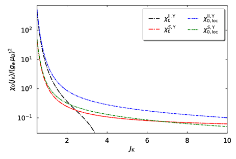
Figure 1: (Color online) Zero-field impurity spin susceptibility $\chi_{0}^{S,{\rm Y}}/(g_{e}\mu_{\rm B})^{2}$, eqs. (65) and (66) and zero-field impurity-induced susceptibility $\chi_{0}^{\rm ii,Y}/(g_{e}\mu_{\rm B})^{2}$, eqs. (LABEL:eq:chiiiYosidaresult) and (71), for global/local magnetic fields as a function of $J_{\rm K}$ of the one-dimensional symmetric Kondo model from the Yosida wave function. The zero-field impurity-induced susceptibility becomes negative at $J_{\rm K}=J_{\rm K,c}^{\rm Y}\approx 3.7543$.

In Fig. 1 we show the corresponding zero-field susceptibilities. They all display an exponential increase for small $J_{\rm K}$, and only differ in the pre-exponential factor. For the impurity spin susceptibility in the Yosida wave function, this factor is proportional to $J_{\rm K}$ and also numerically small, see eq. (67). Therefore, the impurity spin susceptibility is substantially smaller than the impurity-induced susceptibility; this is an artifact of the Yosida wave function.

For large Kondo couplings, $J_{\rm K}>1$, the impurity-induced susceptibility becomes negative for $J_{\rm K}>J_{\rm K,c}^{\rm Y}$, i.e., the Yosida state becomes unstable against a state with a locally broken symmetry. The other susceptibilities remain positive for all $J_{\rm K}$. The impurity spin susceptibility becomes constant for large $J_{\rm K}$, see eq. (68) which is at odds with the exact solution. The local susceptibilities are qualitatively correct for large couplings inasmuch they decay to zero for strong couplings, see eqs. (69) and (75). In fact, the impurity spin susceptibility from the Yosida wave function in the presence of a local field, $\chi_{0,{\rm loc}}^{S,{\rm Y}}(J_{\rm K})$, eq. (69), becomes exact in the limit of strong coupling, see Sect. IX.

VI Gutzwiller wave function

As the third and last analytic variational approach, we study the Gutzwiller wave function. It becomes exact in the limit of large Kondo couplings and provides a very good variational upper bound for the ground-state energy for all Kondo couplings. However, for weak couplings it describes a symmetry-broken state with an oriented moment on the impurity, and a transition to the paramagnetic state at $J_{\rm K,c}^{\rm G}$ that is not contained in the exact solution of the model.

VI.1 Gutzwiller variational state

We define the Gutzwiller variational state Gutzwiller (1964); Linneweber et al. (2017)

$$|\Psi_{\rm G}\rangle=\hat{P}_{\rm G}|\Phi\rangle\;,$$ (76)

where $|\Phi\rangle$ is a normalized single-particle product state to be determined variationally. At half band filling we have

$$n_{\sigma}^{d,0}=\langle\Phi|\hat{n}_{\sigma}^{d}|\Phi\rangle=\frac{1}{2}+\sigma_{n}m\;,$$ (77)

where $\sigma_{n}=1$ for $\sigma=\uparrow$ and $\sigma_{n}=-1$ for $\sigma=\downarrow$, and $0\leq m<1/2$ is the impurity spin polarization in the single-particle product state $|\Phi\rangle$,

$$m=\frac{1}{2}\langle\Phi|\hat{n}_{\uparrow}^{d}-\hat{n}_{\downarrow}^{d}|\Phi\rangle\;.$$ (78)

For a complete Gutzwiller projection, we choose

$$\hat{P}_{\rm G}=\lambda_{\uparrow}\hat{m}_{\uparrow}^{d}+\lambda_{\downarrow}\hat{m}_{\downarrow}^{d}\quad,\quad\hat{m}_{\sigma}^{d}=\hat{n}_{\sigma}^{d}(1-\hat{n}_{\bar{\sigma}}^{d})\;,$$ (79)

where we use $\bar{\uparrow}=\downarrow$ and $\bar{\downarrow}=\uparrow$. Moreover, we demand

$$\hat{P}_{\rm G}^{2}=1+x(\hat{n}_{\uparrow}^{d}-n_{\uparrow}^{d,0})(\hat{n}_{\downarrow}^{d}-n_{\downarrow}^{d,0})\;.$$ (80)

Thus, we have to solve

$$\lambda_{\uparrow}^{2}\hat{m}_{\uparrow}^{d}+\lambda_{\downarrow}^{2}\hat{m}_{\downarrow}^{d} = \lambda_{\uparrow}^{2}\hat{n}_{\uparrow}^{d}+\lambda_{\downarrow}^{2}\hat{n}_{\downarrow}^{d}-(\lambda_{\uparrow}^{2}+\lambda_{\downarrow}^{2})\hat{n}_{\uparrow}^{d}\hat{n}_{\downarrow}^{d}$$ (81)

$$\stackrel{{\scriptstyle!}}{{=}} 1+x(\hat{n}_{\uparrow}^{d}-n_{\uparrow}^{d,0})(\hat{n}_{\downarrow}^{d}-n_{\downarrow}^{d,0})\;.$$

The solution reads

$$x = -\frac{1}{n_{\uparrow}^{d,0}n_{\downarrow}^{d,0}}=-\frac{4}{1-4m^{2}}\;,$$

$$\lambda_{\sigma}^{2} = \frac{1}{n_{\sigma}^{d,0}}=\frac{2}{1+2\sigma_{n}m}\;.$$ (82)

Before we proceed, we note the useful relations

$$\hat{P}_{\rm G}\hat{d}_{\sigma}^{+}\hat{d}_{\bar{\sigma}}^{\vphantom{+}}\hat{P}_{\rm G} = \lambda_{\sigma}\lambda_{\bar{\sigma}}\hat{d}_{\sigma}^{+}\hat{d}_{\bar{\sigma}}^{\vphantom{+}}\;,$$

$$\hat{P}_{\rm G}(\hat{n}_{\uparrow}^{d}-\hat{n}_{\downarrow}^{d})\hat{P}_{\rm G} = \lambda_{\uparrow}^{2}\hat{m}_{\uparrow}^{d}-\lambda_{\downarrow}^{2}\hat{m}_{\downarrow}^{d}$$ (83)

$$= \frac{\hat{n}_{\uparrow}^{d}}{n_{\uparrow}^{d,0}}-\frac{\hat{n}_{\downarrow}^{d}}{n_{\downarrow}^{d,0}}+2m\frac{\hat{n}_{\uparrow}^{d}\hat{n}_{\downarrow}^{d}}{n_{\uparrow}^{d,0}n_{\downarrow}^{d,0}}\;.$$

VI.2 Ground-state energy

The calculation of expectation values and the variational optimization of the energy functional is presented in appendices A.6 and A.7. It requires the solution of an effective non-interacting single-impurity Anderson model that is characterized by a local hybridization parameter $V$.

VI.2.1 Paramagnetic Gutzwiller state

For $m=0$, the ground-state energy for the non-interacting single-impurity Anderson model is known explicitly for all relevant cases. For example, in one dimension it reads Barcza et al. (2019)

$$e_{0}^{\rm A}(V) = \frac{1}{\pi}\left[-\pi+2v_{+}\arctan\left(\frac{1}{v_{-}}\right)+v_{-}\ln\left(\frac{v_{+}-1}{v_{+}+1}\right)\right]$$ (84)

$$+2(1-v_{+})\;,$$

$$v_{\pm} = \sqrt{\frac{\sqrt{1+4V^{4}}\pm 1}{2}}\;.$$ (85)

The Hellmann-Feynman theorem then gives

$$\frac{\partial e_{0}^{\rm A}(V)}{\partial V}=-\frac{8V}{3J_{\rm K}}\;.$$ (86)

The self-consistency equation (86) defines $V(J_{\rm K})$ as a function of $J_{\rm K}$.

The Gutzwiller variational energy for the Kondo model becomes

$$e_{0}^{\rm G}(J_{\rm K})=e_{0}^{\rm A}(V(J_{\rm K}))+\frac{4\left[V(J_{\rm K})\right]^{2}}{3J_{\rm K}}\;.$$ (87)

In general, the Gutzwiller variational energy for the Kondo model must be determined numerically.

Small Kondo couplings.

For $J_{\rm K}\ll 1$ and thus $V\ll 1$ we can approximate

$$e_{0}^{\rm A}(V\ll 1)\approx\frac{2V^{2}}{\pi}\left(\ln(V^{2}/2)-1\right)$$ (88)

in one dimension so that the self-consistency equation (86) becomes

$$-\frac{2\pi}{3J_{\rm K}}=\ln(V^{2}/2)\;,\;V^{2}=2\exp\left(-\frac{2\pi}{3J_{\rm K}}\right)\;.$$ (89)

Therefore, the Gutzwiller estimate for the ground-state energy at small Kondo couplings becomes

$$e_{0}^{\rm G}(J_{\rm K}\ll 1)=-\frac{4}{\pi}\exp\left(-\frac{2}{3\rho_{0}(0)J_{\rm K}}\right)\;.$$ (90)

This is much smaller than the Yosida energy eq. (62), and even smaller than the value for the Yosida-Yoshimori wave function, Yosida (1996); Yosida and Yoshimori (1973)

$$e_{0}^{\rm Y,Y}(J_{\rm K}\ll 1)\sim-\exp\left(-\frac{1}{\rho_{0}(0)J_{\rm K}}\right)\;.$$ (91)

This is not surprising because both variational states miss the actually quadratic dependence of the ground-state energy on $J_{\rm K}$ for small interaction strengths, $e_{0}(J_{\rm K})\sim-J_{\rm K}^{2}$, see eq. (34).

Large Kondo couplings.

For $J_{\rm K}\gg 1$ we can approximate

$$e_{0}^{\rm A}(V\gg 1)\approx-2V+1-\frac{1}{2V}+\frac{2}{3\pi V^{2}}-\frac{1}{16V^{3}}+{\cal O}(1/V^{5})$$ (92)

in one dimension. The self-consistency equation (86) becomes

$$-\frac{4V}{3J_{\rm K}} = -1+\frac{1}{4V^{2}}-\frac{2}{3\pi V^{3}}+\frac{3}{32V^{4}}+{\cal O}(1/V^{6})\;,$$

$$V = \frac{3J_{\rm K}}{4}-\frac{1}{3J_{\rm K}}+\frac{32}{27\pi J_{\rm K}^{2}}-\frac{14}{27J_{\rm K}^{3}}+{\cal O}(1/J_{\rm K}^{5})\;.$$

Therefore, the Gutzwiller estimate for the ground-state energy at large Kondo couplings reads

$$e_{0}^{\rm G}(J_{\rm K}\gg 1)=-\frac{3J_{\rm K}}{4}+1-\frac{2}{3J_{\rm K}}+\frac{32}{27\pi J_{\rm K}^{2}}-\frac{8}{27J_{\rm K}^{3}}\;,$$ (94)

up to and including third order in $1/J_{\rm K}$. This is much smaller than the Yosida energy (64) and is actually exact, up to corrections of the order $1/J_{\rm K}$, see eq. (42). Below, we argue that the first-order and second-order corrections in $1/J_{\rm K}$ are also exact.

The local spin correlation is obtained from the variational Hellmann-Feynman theorem. For large $J_{\rm K}$ we find

$$C_{0}^{S,{\rm G}}(J_{\rm K}\gg 1)=-\frac{3}{4}+\frac{2}{3J_{\rm K}^{2}}-\frac{64}{27\pi J_{\rm K}^{3}}+{\cal O}(1/J_{\rm K}^{4})\;.$$ (95)

VI.2.2 Magnetic Gutzwiller state for weak coupling

As shown in appendix A.7, the numerical optimization of the variational parameters leads to

$$e_{0}^{\rm G}(J_{\rm K})\approx-0.0905J_{\rm K}^{2}-0.051J_{\rm K}^{3}-0.05J_{\rm K}^{4}$$ (96)

for the Gutzwiller variational energy for $J_{\rm K}\lesssim 0.4$.

The quadratic coefficient from the magnetic Gutzwiller wave function can be compared with the exact result from perturbation theory, $e_{0}(J_{\rm K})\approx-3J_{\rm K}^{2}/32=-0.09375J_{\rm K}^{2}$, see eq. (34). The magnetic Gutzwiller states accounts for 96.5% of the correlation energy. Hence, the magnetic Gutzwiller provides an excellent energy estimate but fails to describe the physics properly because it breaks the local symmetry, $m>0$ for $B=0^{+}$.

VI.3 Zero-field susceptibilities

The calculations are carried out in appendix A.8. Here, we summarize the results for the various zero-field susceptibilities in the strong-coupling limit.

VI.3.1 Five equations

The calculation of the zero-field susceptibilities from the Gutzwiller wave function requires the solution of a $5\times 5$ matrix problem,

$$\underline{\underline{M}}\cdot\underline{v}=\underline{g}\;,$$ (97)

where $\underline{g}_{\rm loc}^{\rm T}=(1,0,0,0,0)$ for a local field, and $\underline{g}^{\rm T}=(1,0,g_{3},g_{4},g_{5})$ for a global field whose non-trivial entries $g_{3},g_{4},g_{5}$ are known functions of $V$, and $V(J_{\rm K})$ follows from eq. (86), see appendix A.8. Likewise, the entries of the $5\times 5$ matrix $\underline{\underline{M}}$ are known functions of $V$ and $J_{\rm K}$. The vector

$$\underline{v}=\left(\begin{array}[]{@{}c@{}}\bar{\omega}_{p}\\ \bar{E}_{d}\\ \bar{K}\\ \bar{M}_{0}\\ \chi\end{array}\right)$$ (98)

contains the five unknowns that determine the susceptibilities,

$$\frac{\chi_{0}^{S,{\rm G}}(J_{\rm K},B)}{(g_{e}\mu_{\rm B})^{2}} = \chi\;,$$ (99)

$$\frac{\chi_{0}^{\rm ii,G}(J_{\rm K})}{(g_{e}\mu_{\rm B})^{2}} = \frac{\bar{E}_{d}}{2\pi V^{2}}\;.$$ (100)

The choice of $\underline{g}$ determines whether the external field is applied globally or locally.

Although Mathematica Wolfram Research, Inc. (2016) provides an analytic solution of the linear problem, the expressions are very lengthy and not illuminating. Eventually, we evaluate them numerically.

VI.3.2 Strong-coupling limit

As shown in appendix A.8, compact results can be obtained for $J_{\rm K}\gg 1$. For the zero-field impurity spin susceptibility we find

$$\frac{\chi_{0}^{S,{\rm G}}(J_{\rm K}\gg 1)}{(g_{e}\mu_{\rm B})^{2}} = \frac{20}{9\pi J_{\rm K}^{2}}+{\cal O}(1/J_{\rm K}^{4})\;,$$ (101)

$$\frac{\chi_{0,{\rm loc}}^{S,{\rm G}}(J_{\rm K}\gg 1)}{(g_{e}\mu_{\rm B})^{2}} = =\frac{1}{2J_{\rm K}}+\frac{28}{27J_{\rm K}^{3}}+{\cal O}(1/J_{\rm K}^{4})$$ (102)

in the presence of a global and a local field, respectively.

For the zero-field impurity-induced susceptibilities, the Gutzwiller result for strong coupling reads

$$\frac{\chi_{0}^{\rm ii,G}(J_{\rm K}\gg 1)}{(g_{e}\mu_{\rm B})^{2}} = \frac{8}{9\pi J_{\rm K}^{2}}+\frac{416}{81\pi^{2}J_{\rm K}^{3}}+{\cal O}(1/J_{\rm K}^{4})\;,$$ (103)

$$\frac{\chi_{0,{\rm loc}}^{\rm ii,G}(J_{\rm K}\gg 1)}{(g_{e}\mu_{\rm B})^{2}} = \frac{20}{9\pi J_{\rm K}^{2}}+{\cal O}(1/J_{\rm K}^{4})$$ (104)

in the presence of a global and a local field, respectively.

Since the Gutzwiller wave function becomes exact state for strong coupling, we argue that these results are correct to the indicated order. We shall confirm this assessment from the comparison with numerically exact data from NRG and DMRG in Sect. IX.3.

VI.3.3 Critical interaction for the magnetic transition

For $J_{\rm K}>J_{\rm K,c}^{\rm G}$, the Gutzwiller state describes a spin-isotropic state at the impurity site. For $J_{\rm K}<J_{\rm K,c}^{\rm G}$, the local spin symmetry in the Gutzwiller state is spontaneously broken, i.e., $m>0$ is optimal even at $B=0^{+}$.

With the help of the zero-field spin susceptibility, the transition can accurately be identified because the determinant of the matrix $\underline{\underline{M}}(J_{\rm K})$ changes sign at $J=J_{\rm K,c}^{\rm G}$. Using Mathematica, Wolfram Research, Inc. (2016) the determinant as a function of $V$ can be calculated analytically but the expressions are lengthy. The solution of

$$\det\left(\underline{\underline{M}}(V_{\rm c})\right)=0$$ (105)

is $V_{\rm c}=0.4559222509954975$ with $\det\left(\underline{\underline{M}}(V_{\rm c})\right)=-3.8\cdot 10^{-15}$, or

$$J_{\rm K,c}^{\rm G}=0.8392762432533198\;.$$ (106)

VI.3.4 Comparison of susceptibilities

The paramagnetic Gutzwiller state is stable only for $J_{\rm K}>J_{\rm K,c}^{\rm G}\approx 0.839$ so that we focus on $J_{\rm K}\geq 1$. Since the Gutzwiller wave function becomes exact for $J_{\rm K}\to\infty$, all susceptibilities are positive and well behaved.

In Fig. 2 we show the global and local zero-field susceptibilities. As seen from the figure, the asymptotic formulae for the impurity spin susceptibilities, eqs. (101), (102), (103), and (104), are applicable for $J_{\rm K}\gtrsim 4$.

Fig. 2 also shows that the equivalence

$$\chi_{0}^{S,{\rm G}}(J_{\rm K})=\chi_{0,{\rm loc}}^{\rm ii,G}(J_{\rm K})$$ (107)

holds for all $J_{\rm K}>1$. Therefore, the Gutzwiller approach respects the exact relation (24) at zero temperature. Indeed, as seen from the derivation in Sect. A.7, the Gutzwiller approach solves an effective non-interacting single-impurity Anderson model for which the exact relation eq. (24) is readily shown to hold, too.

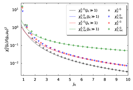
Figure 2: (Color online) Zero-field impurity spin susceptibility $\chi_{0}^{S,{\rm G}}/(g_{e}\mu_{\rm B})^{2}$, eq. (99), and zero-field impurity-induced susceptibility $\chi_{0}^{\rm ii,G}/(g_{e}\mu_{\rm B})^{2}$, eq. (100), for global/local magnetic fields as a function of $J_{\rm K}\geq 1$ of the one-dimensional symmetric Kondo model from the Gutzwiller wave function. For comparison, we also include the limiting behavior for the susceptibilities, eqs. (101), (102), (103), and (104).

VII Bethe Ansatz results

Using Bethe Ansatz, the Kondo model is solved for a linear dispersion relation with unit Fermi velocity in the wide-band limit, i.e., the dispersion relation $\epsilon^{\rm BA}(k)=k$ formally extends from $k_{-}=-\infty$ to $k_{+}=+\infty$. Therefore, an appropriate energy cut-off $D$ must be introduced in the Bethe Ansatz equations. This procedure is not unique. Therefore, there are two Bethe Ansatz solutions for the spin-1/2 Kondo model. First, the one discussed by Tsvelick and Wiegmann, referred to as TW, Tsvelick and Wiegmann (1983) and, second, the one reviewed by Andrei, Furuya, and Lowenstein, referred to as AFL. Andrei et al. (1983) The basic Bethe Ansatz equations agree but the expressions for the parameters as a function of the Bethe Ansatz Kondo coupling $J_{\rm K}^{\rm BA}/D$ differ beyond leading-order. For a lattice-regularized Bethe-Ansatz solvable impurity model, see Ref. [Bortz and Klümper, 2004].

In this section we discuss the Bethe Ansatz results for the zero-field impurity-induced susceptibility and magnetization. As shown in appendix B.5, the Bethe Ansatz solution leads to

$$e_{0}^{\rm BA}(J_{\rm K}^{\rm BA})={\cal O}\left(\left(J_{\rm K}^{\rm BA}\right)^{3}\right)\;.$$ (108)

Thus, the Bethe Ansatz results cannot be used for comparison with the ground-state energy of the Kondo impurity on a chain.

VII.1 Zero-field impurity-induced magnetic susceptibility

The Bethe Ansatz leads to equation (4.30) of AFL Andrei et al. (1983) or equation (5.1.23) of TW Tsvelick and Wiegmann (1983) for the zero-field magnetic susceptibility

$$\frac{\chi^{\rm ii}_{0}(J_{\rm K})}{\left(g_{e}\mu_{\rm B}\right)^{2}}=\frac{1}{4\pi T_{0}(J_{\rm K}^{\rm BA})}$$ (109)

in the limit of small $J_{\rm K}^{\rm BA}$ for a half-filled system.

The Bethe Ansatz solves the Kondo model for a Kondo interaction strength $J_{\rm K}^{\rm BA}$ in the limit of an infinite bandwidth. To arrive at tangible results, a symmetric bandwidth cutoff, $|\epsilon|<D$, is imposed on the Bethe Ansatz equations, and periodic boundary conditions are implemented so that the electron density remains finite, $D_{\rm AFL}\equiv N^{e}/L=1/2$ at half band-filling, see appendix B.5. The corresponding bandwidth is $W^{\rm BA}=2D$ with

$$D\equiv K_{\rm AFL}=\pi D_{\rm AFL}=\frac{\pi}{2}$$ (110)

so that the density of states is given by

$$\rho_{0}=\frac{1}{2D}=\frac{1}{\pi}$$ (111)

at the Fermi energy $E_{\rm F}=0$, and for all $|\epsilon|\leq D$. Then, the low-temperature magnetic energy scale from Bethe Ansatz is given by

$$T_{0}(J_{\rm K}^{\rm BA})=\frac{D}{\pi}\exp\left(-\frac{1}{\rho_{0}J_{\rm K}^{\rm BA}}\right)\;.$$ (112)

The remaining problem is to express $T_{0}(J_{\rm K}^{\rm BA})$ as a function of $J_{\rm K}$, or, equivalently, to find an explicit relation between $J_{\rm K}^{\rm BA}$ and $J_{\rm K}$. The existence of such a unique relation is thoroughly discussed in Sect. VI of AFL. Andrei et al. (1983)

VII.2 Wilson’s renormalization group

Wilson’s renormalization group Wilson (1975) for the Kondo model starts from the lattice model in the thermodynamic limit with its energy cut-off parameter ${\cal D}=W/2=1$ and Kondo coupling $J_{\rm K}$. By successively integrating out the high-energy degrees of freedom, the renormalization group flows to the Bethe Ansatz model with a linear dispersion relation around the Fermi energy and the coupling $J_{\rm K}^{\rm BA}$.

The renormalization group (RG) transformation is actually performed on the Hamiltonian as well as on the matrix representation of the operators, both influencing the physical quantities such as the zero-field impurity-induced susceptibility. In his review, eq. (IX.91) on p. 835, Wilson (1975) Wilson provides the general series expansion for the zero-field impurity-induced susceptibility at zero temperature,

$$\frac{\chi_{0}^{\rm ii}(J_{\rm K})}{(g_{e}\mu_{\rm B})^{2}} = \frac{w}{4\widetilde{D}(j)}\frac{\exp\left(1/j\right)}{\sqrt{j}}\exp\biggl{(}-\alpha_{1}j-\sum_{n=2}^{\infty}\alpha_{n}j^{n}\biggr{)}\;,$$

$$\frac{\widetilde{D}(j)}{{\cal D}} = c_{0}+\sum_{n=1}^{\infty}c_{n}j^{n}\;,\quad j=\rho_{0}(0)J_{\rm K}\;,$$ (113)

where $\rho_{0}(0)$ is the density of states at the Fermi energy. In Ref. [Wilson, 1975], $\alpha_{1}$ and $w$ were determined numerically for a constant density of states, $w/4\approx 0.1032$, and $\alpha_{1}=1.5824$. AFL calculated the Wilson number $w$ analytically, Andrei et al. (1983)

$$w=\frac{w_{\rm AFL}}{\pi}=\frac{e^{\gamma_{\rm E}+1/4}}{\pi^{3/2}}\approx 0.410705$$ (114)

with Euler’s constant $\gamma_{\rm E}\approx 0.577216$. We concisely re-derive $w$ in appendix B.6.

The coefficients $c_{n}$ in eq. (113) can be obtained from the high-temperature expansion of the zero-field impurity-induced susceptibility. To third order it reads, see eq. (IX.57) of Ref. [Wilson, 1975],

$$\frac{4T\chi_{0}^{\rm ii}(T,J_{\rm K})}{(g_{e}\mu_{\rm B})^{2}} \approx 1-j+j^{2}\ln(T/\widetilde{D}(j))$$

$$-j^{3}\left[\left(\ln(T/\widetilde{D}(j))\right)^{2}+\frac{1}{2}\ln(T/\widetilde{D}(j))\right]\;.$$

Indeed, to second order the comparison of eq. (VI-78) of the supplemental material with eq. (VII.2) gives

$$\frac{\widetilde{D}(j)}{{\cal D}}\approx\frac{UC}{2}\equiv c_{0}$$ (116)

with

$$U=\frac{e^{3/4+\gamma_{\rm E}}}{\pi}=\sqrt{\pi e}w$$ (117)

from eq. (VI-58) and $C$ from eq. (60). Thus, the prefactor of the susceptibility in eq. (113) to leading order reads

$$\frac{w}{4\widetilde{D}(j)}\approx\frac{w}{2UC{\cal D}}=\frac{1}{2{\cal D}C\sqrt{\pi e}}\;.$$ (118)

This result does not contain the Wilson number but only the prefactor $1/(2{\cal D}C\sqrt{\pi e})$. This does not come as a surprise because we consider finite magnetic fields at zero temperature while $T_{\rm K}$ characterizes the zero-field susceptibility at finite temperatures. Note that the prefactor $c_{0}$ in eq. (116) contains information about the host-electron density of states via the regularized first negative moment (60).

As shown in AFL, Andrei et al. (1983) and re-derived in Appendix B.6, the Kondo temperature $T_{\rm K}$ and the magnetic energy scale $T_{\rm H}=\sqrt{\pi/e}T_{0}$ are related by

$$T_{\rm K}=UT_{\rm H}\;,$$ (119)

with corrections of the order $\rho_{0}(0)J_{\rm K}$. Using eqs. (109), (112), (113), and (118), we find

$$T_{\rm K}=w\sqrt{\pi e}\frac{{\cal D}C}{2}\sqrt{\rho_{0}(0)J_{\rm K}}\exp\left(-\frac{1}{\rho_{0}(0)J_{\rm K}}\right)\;,$$ (120)

with corrections of the order $\rho_{0}(0)J_{\rm K}$. Thus, in eq. (109)

$$\frac{\chi^{\rm ii}_{0}(J_{\rm K})}{(g_{e}\mu_{\rm B})^{2}}=\frac{w}{4T_{\rm K}}\;,$$ (121)

which is the familiar expression of the zero-temperature susceptibility in terms of the Kondo temperature $T_{\rm K}$, see eq. (4.58) of Hewson’s book. Hewson (1993)

In general, eq. (113) can be cast into the form

$$\frac{\chi_{0}^{\rm ii}(J_{\rm K})}{(g_{e}\mu_{\rm B})^{2}} = s_{0}\frac{\bar{\chi}_{0}(j)}{(g_{e}\mu_{\rm B})^{2}}\left(1+\sum_{n=1}^{\infty}\frac{s_{n}}{s_{0}}j^{n}\right)\;,\;j=\rho_{0}(0)J_{\rm K}\;,$$

$$\frac{\bar{\chi}_{0}(j)}{(g_{e}\mu_{\rm B})^{2}} = \frac{\exp\left(1/j\right)}{\sqrt{j}}\;,\quad s_{0}=\frac{1}{2{\cal D}C\sqrt{\pi e}}\;.$$ (122)

To go beyond the leading order, i.e., to determine the coefficient $s_{1}$ in eq. (122) analytically, requires the cumbersome calculation of the ground-state energy as a function of magnetic field $B$ to third order in $\rho_{0}(0)J_{\rm K}$. This is beyond the scope of our presentation.

The comparison of the zero-field impurity-induced susceptibility from the renormalization group in eq. (122) with the corresponding Bethe-Ansatz expressions (109) and (112) leads to the desired relation between $(D,J_{\rm K}^{\rm BA})$ and $({\cal D},J_{\rm K})$,

$$\frac{1}{\rho_{0}J_{\rm K}^{\rm BA}} = \frac{1}{\rho_{0}(0)J_{\rm K}}-\frac{1}{2}\ln\left(\rho_{0}(0)J_{\rm K}\right)+\ln\left(\sqrt{\frac{1}{\pi e}}\frac{2D}{C{\cal D}}\right)$$ (123)

$$+\ln\biggl{[}1+\sum_{n=1}^{\infty}\frac{s_{n}}{s_{0}}\left(\rho_{0}(0)J_{\rm K}\right)^{n}\biggr{]}$$

with ${\cal D}=W/2=1$ for the lattice model and $D=\pi/2$ in the Bethe-Ansatz solvable model.

VII.3 Impurity-induced magnetization

The Bethe Ansatz provides the impurity-induced magnetization of the system $m^{\rm ii}(J_{\rm K}^{\rm BA},B,T)$ at finite temperatures $T$ and finite external fields $B$, see eq. (19). For small couplings, $J_{\rm K}\ll 1$, the impurity-induced susceptibility is exponentially large, see eq. (122), so that the relevant magnetic fields that lead to a finite magnetization are exponentially small. The polarization of the host electrons becomes negligibly small, and we do not have to distinguish between the impurity spin polarization and the impurity-induced magnetization, i.e., $m^{\rm ii}(J_{\rm K}\ll 1,B\to 0)=m^{S}(J_{\rm K}\ll 1,B\to 0)$, with exponential accuracy. Therefore, the zero-field susceptibilities from the impurity-induced magnetization and from the impurity spin polarization become identical.

From eqs. (5.1.34) and (5.1.37) in TW and (4.29) in AFL, the Bethe Ansatz result for the impurity-induced magnetization reads ($e=\exp(1)$)

$$\frac{m^{\rm ii}(h\leq 1)}{g_{e}\mu_{\rm B}} = \frac{1}{2\sqrt{\pi}}\sum_{n=0}^{\infty}\left(\frac{n+1/2}{e}\right)^{n+1/2}\frac{(-1)^{n}h^{2n+1}}{n!(n+1/2)}\;,$$

$$\frac{m^{\rm ii}(h\geq 1)}{g_{e}\mu_{\rm B}} = \frac{1}{2}-\frac{1}{2\pi^{3/2}}\int_{0}^{\infty}{\rm d}\omega\frac{\sin(\pi\omega)}{\omega}\Gamma(1/2+\omega)$$ (125)

$$\hphantom{\frac{1}{2}-\frac{1}{2\pi^{3/2}}\int_{0}^{\infty}}\times\left(\frac{\omega}{e}\right)^{-\omega}h^{-2\omega}\;.$$

In eqs. (LABEL:eq:hsmallerthanunity) and (125), the external field is scaled by the universal low-temperature magnetic energy scale $T_{1}$,

$$h = \frac{B}{T_{1}}\;,$$

$$T_{1} = \sqrt{\frac{2\pi}{e}}T_{0}=\sqrt{\frac{2\pi}{e}}\left(\frac{4\pi\chi_{0}^{\rm ii}(J_{\rm K})}{(g_{e}\mu_{\rm B})^{2}}\right)^{-1}\;.$$ (126)

Since $\chi^{\rm ii}_{0}(J_{\rm K})$ can be calculated analytically in terms of $\rho_{0}(0)J_{\rm K}$ only to leading order, see eq. (123), we follow the usual approach and determine $T_{1}$ numerically from the zero-field susceptibility. Höck and Schnack (2013)

VIII Numerical approaches

In this section, we briefly discuss two numerically exact approaches to the many-body problem. We begin with the Density-Matrix Renormalization Group (DMRG) method, and move on to the Numerical Renormalization Group (NRG) technique that performs the Wilson renormalization scheme numerically.

VIII.1 DMRG

VIII.1.1 Impurity spin polarization and impurity-induced magnetization

Impurity spin polarization

When we apply the magnetic field only at the impurity, standard DMRG ground-state calculations provide the results for the impurity spin polarization $\langle\hat{S}^{z}\rangle=m_{\rm loc}^{S}/(g_{e}\mu_{\rm B})$. For a globally applied field ${\cal H}$ the calculation of $\langle\hat{S}^{z}\rangle$ is more subtle because the total spin in $z$-direction $S_{\rm tot}^{z}=S^{z}+s^{z}$ is a good quantum number, Barcza et al. (2019) see Sect. II.2.2. Therefore, the spin quantum number $S_{\rm tot}^{z}$ changes from $S_{\rm tot}^{z}=0$ for ${\cal H}=0$ to $S_{\rm tot}^{z}=1,2,3,\ldots$ for increasing external fields in steps of $g\mu_{\rm B}{\cal H}_{n}$ whenever

$$g\mu_{\rm B}{\cal H}_{n}=E_{0}(S_{\rm tot}^{z}=n)-E_{0}(S_{\rm tot}^{z}=n-1)$$ (127)

for $n=1,2,3,\ldots\$. Thus, the impurity spin polarization is recorded only at discrete values of the external field whereby expectation values are calculated with the ground state for $S_{\rm tot}^{z}=n$. For $J_{\rm K}\leq 1$, we use system sizes $L=29,61,125,253,509,637,765$. Since this approach hampers a systematic finite-size extrapolation, we plot $m^{S}(B)/(g_{e}\mu_{\rm B})$ for our largest system sizes.

For $J_{\rm K}\gtrsim 1$ and a global magnetic field, the calculation of the impurity spin polarization faces the problem that the impurity and the electron spin at $n=0$ form a singlet and tend to separate from the rest of the system. This reduces the effective length of the half-chain by one site, and a finite-size gap opens at the Fermi energy. To counteract this effect for $J_{\rm K}\gtrsim 1$, we subtract two sites form the original chain, i.e., we use $L=27,59,123,251,507,635,763$. Then, the ground state at ${\cal H}=0^{+}$ has total spin $S_{\rm tot}^{z}=1/2$, and the impurity magnetization of the ground states at $S_{\rm tot}^{z}=n+1/2$ ($n=1,2,3,\ldots$) is recorded.

Impurity-induced magnetization

In DMRG, we can calculate the ground-state energy $E_{0}(J_{\rm K},S^{z}_{\rm tot},L)$ for given integer $0\leq S^{z}_{\rm tot}\leq(L+3)/2$. For very large system sizes, $\Delta E(J_{\rm K},S^{z}_{\rm tot},L)=E_{0}(J_{\rm K},S^{z}_{\rm tot},L)-E_{0}(J_{\rm K},0,L)$ can be fitted to a positive, continuous function of $s\equiv S^{z}_{\rm tot}$. Then, the global external field is obtained from

$$B=\frac{\partial\Delta E(J_{\rm K},s,L)}{\partial s}\equiv E_{0}^{\prime}(s)\;.$$ (128)

In turn, we may solve eq. (128) for the total spin $s_{\rm opt}(B)$ as a function of $B$,

$$s_{\rm opt}(B)=[E_{0}^{\prime}]^{-1}(B)\;,$$ (129)

where $[E_{0}^{\prime}]^{-1}(x)$ is the inverse function of $E_{0}^{\prime}(x)$ for given $J_{\rm K}$ and $L$. Thus, the impurity-induced magnetization for a global field is given by

$$\frac{m^{\rm ii,DMRG}(J_{\rm K},B,L)}{g_{e}\mu_{\rm B}}=s_{\rm opt}(J_{\rm K},B,L)-s_{\rm opt}^{\rm free}(B,L)\;.$$ (130)

For a local field, one has to also calculate the impurity spin polarization $\langle\hat{S}^{z}\rangle$ as a function of $S_{\rm tot}^{z}$.

In practice, it requires exceedingly large system sizes to carry out this program because, in the region of small Kondo couplings, $J_{\rm K}\lesssim 0.5$, the susceptibility is very large so that the system is almost fully polarized for very small fields even for system sizes $L={\cal O}(10^{3})$. For this reason the analytic curve $E_{0}(s)$ is not known with the required accuracy. Therefore, we do not employ the DMRG to calculate impurity-induced quantities.

VIII.1.2 Technicalities

The accuracy of the calculations is controlled using the dynamic block-state selection (DBSS) scheme. Legeza et al. (2003); Legeza and Sólyom (2004) Setting the control parameter to $\chi=10^{-5}$, the truncation error yields around $10^{-7}$ while the number of maximally kept DMRG block-states was observed to in the range $M=5000$ for our largest system sizes.

For the ground-state energy we use DMRG to calculate the excess ground-state energy $e_{0}(J_{\rm K},L)$, see eq. (9), and extrapolate to the thermodynamic limit,

$$e_{0}^{\rm DMRG}(J_{\rm K})=\lim_{L\to\infty}e_{0}^{\rm DMRG}(J_{\rm K},L)$$ (131)

using a second-order polynomial fit in $1/L$. As an example, we present the ground-state energy $e_{0}^{\rm DMRG}(J_{\rm K},L)$ and the local spin-correlation $C_{0}^{S,{\rm DMRG}}(J_{\rm K},L)$ as a function of inverse system size for $J_{\rm K}=0.1,0.5,1$ in Fig. 3; the finite-size extrapolation is unproblematic.

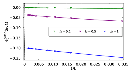
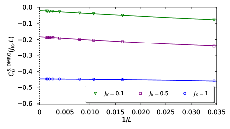
Figure 3: (Color online) Ground-state energy $e_{0}^{\rm DMRG}(J_{\rm K},L)$ from DMRG (upper figure) and local spin correlation function $C_{0}^{S,{\rm DMRG}}(J_{\rm K},L)$ (lower figure) of the one-dimensional symmetric Kondo model as a function of inverse system size $1/L$ for $J_{\rm K}=0.1,0.5,1$. The solid lines represent the second-order polynomial fit in $1/L$.

In Fig. 4 we show the zero-field impurity spin susceptibility $\chi_{0}^{\rm S,DMRG}(J_{\rm K},L)$ for a global magnetic field and $\chi_{0,{\rm loc}}^{\rm S,DMRG}(J_{\rm K},L)$ for a local magnetic field on a logarithmic scale as a function of inverse system size $1/L$ for $J_{\rm K}=0.6,1,5$. Apparently, the finite-size extrapolation can safely be performed for the zero-field impurity spin susceptibility for moderate to large coupling strengths, $J_{\rm K}\gtrsim 0.6$, because the NRG data are reasonably well reproduced.

As in the case of the single-impurity Anderson model, Barcza et al. (2019) the DMRG calculations for a global magnetic field are troubled for small Kondo couplings. This is shown in Fig. 5 for $J_{\rm K}=0.4,0.5,0.6$. For $J_{\rm K}\ll 1$, it requires exponentially increasing system size to resolve the exponentially small energy scale for spin excitations, i.e., for $J_{\rm K}\lesssim 0.5$, a reliable extrapolation of the susceptibility to the thermodynamic limit requires system sizes that already exceed $L=10^{3}$ by far. For a local magnetic field, the DMRG can access low fields so that the zero-field impurity spin susceptibility is much better behaved at small interactions. Nevertheless, the extrapolation is not very stable, as can be seen from the winding fitting curves, and the NRG values cannot be recovered faithfully. Again, for $J_{\rm K}\lesssim 0.5$ a reliable extrapolation of the DMRG values for the zero-field impurity spin susceptibility to the thermodynamic limit requires exponentially large system sizes.

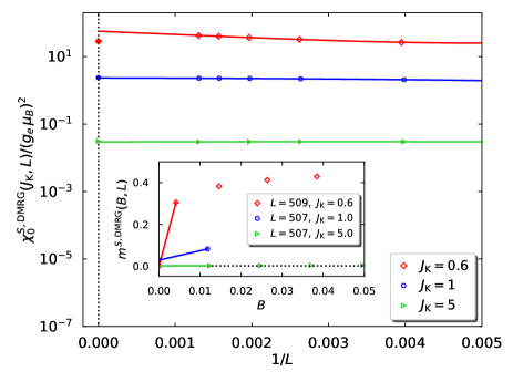
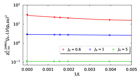
Figure 4: (Color online) Zero-field impurity spin susceptibility $\chi_{0}^{S,{\rm DMRG}}(J_{\rm K},L)$ from DMRG for a global magnetic field (upper figure) and $\chi_{0,{\rm loc}}^{S,{\rm DMRG}}(J_{\rm K},L)$ for a local magnetic field (lower figure) on a logarithmic scale for the one-dimensional symmetric Kondo model as a function of inverse system size $1/L$ for $J_{\rm K}=0.6,1,5$. For comparison, data from NRG are shown as filled symbols at $1/L=0$. The solid lines represent the second-order polynomial fit in $1/L$ on the logarithm of the susceptibility. The inset shows the magnetization $m^{S,{\rm DMRG}}(J_{\rm K},B,L=507,509)$ as a function of a small applied field whose slope defines $\chi_{0}^{S,{\rm DMRG}}(J_{\rm K},L)/(g_{e}\mu_{\rm B})^{2}\approx[m^{S,{\rm DMRG}}(J_{\rm K},B_{1},L)-m^{S,{\rm DMRG}}(J_{\rm K},0,L)]/(2B_{1})$.

VIII.2 NRG

Here, we compile basic information about the NRG algorithm that we employ in our work; for a review on NRG, see Ref. [Bulla et al., 2008].

VIII.2.1 Wilson chain

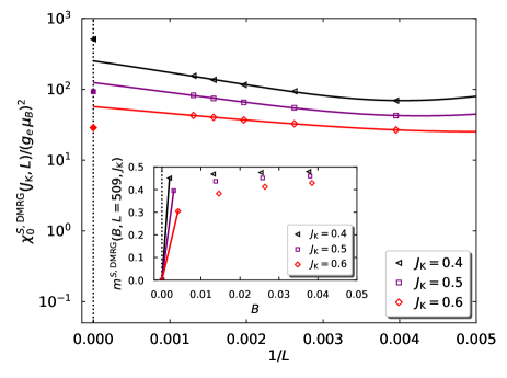
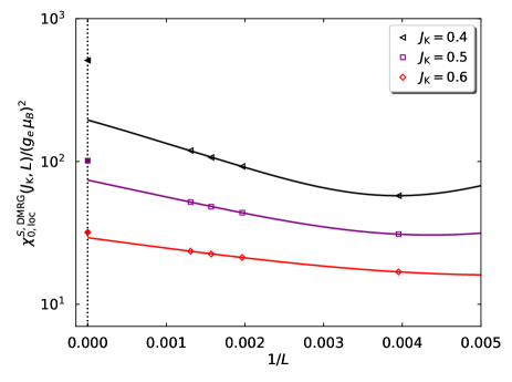
Figure 5: (Color online) Same content as Fig. 4 but for $J_{\rm K}=0.4,0.5,0.6$. Inset: Magnetization $m^{S,{\rm DMRG}}(J_{\rm K},B,L=509)$ as a function of a small applied field for $J_{\rm K}=0.4,0.5,0.6$ whose slope defines $\chi_{0}^{S,{\rm DMRG}}/(g_{e}\mu_{\rm B})^{2}$.

The NRG starts from the energy representation of the Hamiltonian, Höck and Schnack (2013)

$$\hat{H}_{\rm K}=\hat{T}^{\rm NRG}+\hat{V}_{\rm sd}^{\rm NRG}+\hat{H}_{{\rm loc},{\rm m}}\;,$$ (132)

with the kinetic energy

$$\hat{T}^{\rm NRG}=\sum_{\sigma}\int_{-1-\sigma_{n}B}^{1-\sigma_{n}B}{\rm d}\epsilon\,\epsilon\,\tilde{a}_{\epsilon,\sigma}^{+}\tilde{a}_{\epsilon,\sigma}^{\vphantom{+}}\;,$$ (133)

and the local Kondo interaction

$$\hat{V}_{\rm sd}^{\rm NRG} = \frac{1}{2}\left(\hat{f}_{0,\uparrow}^{+}\hat{f}_{0,\downarrow}^{\vphantom{+}}\hat{d}_{\downarrow}^{+}\hat{d}_{\uparrow}^{\vphantom{+}}+\hat{f}_{0,\downarrow}^{+}\hat{f}_{0,\uparrow}^{\vphantom{+}}\hat{d}_{\uparrow}^{+}\hat{d}_{\downarrow}^{\vphantom{+}}\right)$$

$$+\frac{1}{4}\left(\hat{d}_{\uparrow}^{+}\hat{d}_{\uparrow}^{\vphantom{+}}-\hat{d}_{\downarrow}^{+}\hat{d}_{\downarrow}^{\vphantom{+}}\right)\left(\hat{f}_{0,\uparrow}^{+}\hat{f}_{0,\uparrow}^{\vphantom{+}}-\hat{f}_{0,\downarrow}^{+}\hat{f}_{0,\downarrow}^{\vphantom{+}}\right)\;.$$

Here, the electron mode that couples to the impurity is given by

$$\hat{f}_{0,\sigma}=\int_{-1-\sigma_{n}B}^{1-\sigma_{n}B}{\rm d}\epsilon\sqrt{\rho_{0}(\epsilon+\sigma_{n}B)}\tilde{a}_{\epsilon,\sigma}^{\vphantom{+}}\;,$$ (134)

where $\sigma_{n}=1$ for $\sigma=\uparrow$ and $\sigma_{n}=-1$ for $\sigma=\downarrow$. In this step, no approximation is introduced.

The decisive step is the logarithmic discretization of the NRG Hamiltonian (134). In the presence of a global field, the upper and lower band edges differ from each other,

$$W_{\pm,\sigma}=\pm 1-\sigma_{n}B\;.$$ (135)

Thus, we follow Hager Hager (2007); Bulla et al. (2008) and define the sampling points

$$x_{n,\sigma,\pm}=W_{\pm,\sigma}\Lambda^{-n}\;,\;n=0,1,2,\ldots$$ (136)

that depend on the position of the upper ($+$) and lower ($-$) band edges for spin $\sigma=\uparrow,\downarrow$. As usual, Höck and Schnack (2013) we approximate the density of states in each interval $I_{n,\sigma}^{+}=[x_{n+1,\sigma,+},x_{n,\sigma,+}]$ and $I_{n,\sigma}^{-}=[x_{n,\sigma,-},x_{n+1,\sigma,-}]$ by a suitably chosen constant. With the interval width

$$d_{n,\sigma}^{\pm}=\left|W_{\pm,\sigma}\right|\Lambda^{-n}\left(1-\Lambda^{-1}\right)$$ (137)

we define

$$\left(\gamma_{n,\sigma}^{\pm}\right)^{2}=\int_{I_{n,\sigma}^{\pm}}{\rm d}\epsilon\rho_{0}(\epsilon+\sigma_{n}B)$$ (138)

and the expansion operators

$$\tilde{b}_{n,p,\sigma,\pm}^{\vphantom{+}}=\int_{I_{n,\sigma}^{\pm}}{\rm d}\epsilon\frac{1}{\sqrt{d_{n}^{\pm}}}e^{\mp 2\pi{\rm i}p\epsilon/d_{n}^{\pm}}\tilde{a}_{\epsilon,\sigma}^{\vphantom{+}}$$ (139)

such that we can write

$$\hat{f}_{0,\sigma}^{\vphantom{+}}=\sum_{n}\left(\gamma_{n,\sigma}^{+}\tilde{b}_{n,0,\sigma,+}^{\vphantom{+}}+\gamma_{n,\sigma}^{-}\tilde{b}_{n,0,\sigma,-}^{\vphantom{+}}\right)$$ (140)

for the bath state that couples to the impurity. Note that only the mode $p=0$ appears in the bath-electron operator $\hat{f}_{0,\sigma}^{\vphantom{+}}$.

The kinetic energy becomes

$$\hat{T}^{\rm NRG} = \sum_{n,p,p^{\prime},\sigma}\zeta_{n,p,p^{\prime},\sigma}^{+}\tilde{b}_{n,p,\sigma,+}^{+}\tilde{b}^{\vphantom{+}}_{n,p^{\prime},\sigma,+}$$ (141)

$$\hphantom{\sum_{n,p,p^{\prime},\sigma}}+\zeta_{n,p,p^{\prime},\sigma}^{-}\tilde{b}_{n,p,\sigma,-}^{+}\tilde{b}^{\vphantom{+}}_{n,p^{\prime},\sigma,-}\;.$$

To construct the Wilson chain we now drop all modes $p\neq 0$ in the kinetic energy,

$$\hat{T}^{\rm NRG}\approx\sum_{n,\sigma}\zeta_{n,\sigma}^{+}\tilde{b}_{n,\sigma,+}^{+}\tilde{b}^{\vphantom{+}}_{n,\sigma,+}+\zeta_{n,\sigma}^{-}\tilde{b}_{n,\sigma,-}^{+}\tilde{b}^{\vphantom{+}}_{n,\sigma,-}$$ (142)

with $\tilde{b}^{\vphantom{+}}_{n,\sigma,\pm}\equiv\tilde{b}^{\vphantom{+}}_{n,0,\sigma,\pm}$ and

$$\zeta_{n,\sigma}^{\pm}\equiv\zeta_{n,0,0,\sigma}^{\pm}=\frac{\displaystyle\int_{I_{n,\sigma}^{\pm}}{\rm d}\epsilon\,\epsilon\,\rho_{0}(\epsilon+\sigma_{n}B)}{\displaystyle\int_{I_{n,\sigma}^{\pm}}{\rm d}\epsilon\,\rho_{0}(\epsilon+\sigma_{n}B)}\;.$$ (143)

This approximation becomes exact in the limit $\Lambda\to 1$; for a thorough discussion, see Ref. [Bulla et al., 2008].

As a final step in the construction of the Wilson chain, we choose $|0_{\sigma}\rangle\equiv\hat{f}_{0,\sigma}^{+}|\text{vac}\rangle$ as starting vector for the iterative construction of the Lanczos vectors, see appendix B.2. The kinetic energy operator is then represented as a tight-binding Hamiltonian on a chain,

$$\hat{T}^{\rm NRG}=\sum_{n=0,\sigma}^{\infty}\varepsilon_{n,\sigma}\hat{f}_{n,\sigma}^{+}\hat{f}^{\vphantom{+}}_{n,\sigma}+t_{n,\sigma}\left(\hat{f}_{n,\sigma}^{+}\hat{f}^{\vphantom{+}}_{n+1,\sigma}+\text{h.c.}\right)\;.$$ (144)

The matrix elements are calculated according to the equations (28)-(31) in Ref. [Bulla et al., 2008]. For completeness, we give the details in appendix A.9.

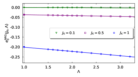
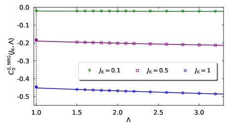
Figure 6: (Color online) Ground-state energy $e_{0}^{\rm NRG}(J_{\rm K},\Lambda)$ from NRG (upper figure) and local spin correlation function $C_{0}^{S,{\rm NRG}}(J_{\rm K},\Lambda)$ (lower figure) of the one-dimensional symmetric Kondo model as a function of the Wilson parameter $\Lambda$ for $J_{\rm K}=0.1,0.5,1$. The solid lines represent a second-order polynomial fit in $(\Lambda-1)$. Filled symbols at $\Lambda=1$ represent the DMRG values.

VIII.2.2 Technicalities

The Wilson chain is solved iteratively, as described in detail in Ref. [Bulla et al., 2008]. As maximal chain length we use $30\leq n_{\rm max}\leq 100$, depending on the value of $J_{\rm K}$. At the end of each diagonalization step in the renormalization group procedure, we keep $3000<N_{s}<5000$ lowest-energy eigenstates.

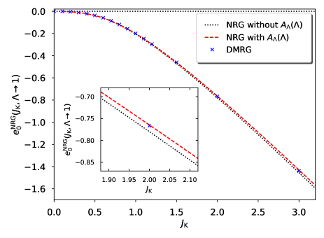
Figure 7: (Color online) Ground-state energy $e_{0}^{\rm NRG}(J_{\rm K},\Lambda)$ from NRG of the one-dimensional symmetric Kondo model as a function of the Kondo coupling $J_{\rm K}$. NRG data with and without the correction factor $A_{\Lambda}(\Lambda)$ were extrapolated to $\Lambda\to 1$. DMRG data are shown for comparison.

At the end of the renormalization group calculation, we thus have $N_{s}$ states with their global quantum numbers (energy, particle number, spin component in $z$ direction) that permit the calculation of thermodynamic quantities such as the ground-state and free energy, impurity-induced magnetization, and magnetic susceptibility by taking the derivative with respect to the external field, see eq. (21). For large couplings, $J_{\rm K}\gtrsim 5$, it is numerically advantageous to calculate the zero-field impurity-induced susceptibility from the second-order derivative of the ground-state energy.

For the calculation of local expectation values, e.g., the local spin correlation and impurity spin polarization, the corresponding quantities are expressed in terms of the Wilson chain operators and are transformed in each renormalization group step.

The discretization parameter $\Lambda$ we choose in the range $1.8\leq\Lambda\leq 3.2$. To include the discretization correction for reconnecting with the original continuum model even for a finite $\Lambda$, we follow Krishna-murthy, Wilkins, and Wilson, Krishna-murthy et al. (1980a, b) and multiply the Kondo coupling with the correction factor

$$A_{\Lambda}(\Lambda)=\frac{1}{2}\frac{\Lambda+1}{\Lambda-1}\ln(\Lambda)$$ (145)

that becomes unity for $\Lambda\to 1$. The factor was derived for a constant density of states but we shall see that it also works very well for the one-dimensional density of states.

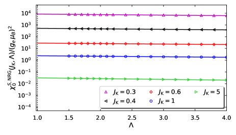
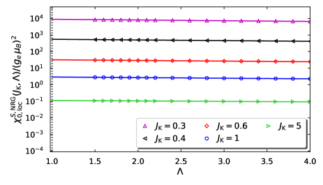
Figure 8: (Color online) Zero-field impurity spin susceptibility $\chi_{0}^{S,{\rm NRG}}(J_{\rm K},\Lambda)$ from NRG for a global magnetic field (upper figure) and $\chi_{0,{\rm loc}}^{S,{\rm NRG}}(J_{\rm K},\Lambda)$ for a local magnetic field (lower figure) for the one-dimensional symmetric Kondo model as a function of the Wilson parameter $\Lambda$ for $J_{\rm K}=0.3,0.4,0.6,1,5$. The solid lines represent the second-order polynomial fit of $\ln[\chi_{0}(\Lambda)]$ in $(\Lambda-1)$.

As an example, we consider the ground-state energy. We calculate $e_{0}^{\rm NRG}(J_{\rm K},\Lambda)$ and extrapolate to the limit $\Lambda\to 1$,

$$e_{0}^{\rm NRG}(J_{\rm K})=\lim_{\Lambda\to 1}e_{0}^{\rm NRG}(J_{\rm K},\Lambda)\;,$$ (146)

using a second-order polynomial fit in $(\Lambda-1)$. In Fig. 6. we present the ground-state energy $e_{0}^{\rm NRG}(J_{\rm K},\Lambda)$ and the local spin-correlation $C_{0}^{S,{\rm NRG}}(J_{\rm K},\Lambda)$ as a function of the Wilson parameter $\Lambda$ for $J_{\rm K}=0.1,0.5,1$.

The extrapolation to $\Lambda\to 1$ provides very good results in comparison with DMRG. Note that it requires $\Lambda$-values as small as $\Lambda=1.8$ to achieve an agreement of the extrapolated NRG values and DMRG data within an accuracy of better than one percent.

For an independent assessment of the quality of the $\Lambda$-extrapolation, we also performed NRG calculations where we switched off the correction factor $A_{\Lambda}(\Lambda)$. Recall that the correction factor was derived for a constant density of states and thus does not necessarily perform perfectly for the one-dimensional density of states. As seen from Fig. 7, the extrapolated values for the ground-state energy differ by less than one percent. In particular, the resulting energy values are slightly below the DMRG values when the correction factor is switched off whereas they remain consistently above the DMRG energies when the correction factor is employed. Therefore, we keep the correction factor in all our NRG calculations.

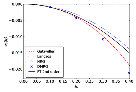
Figure 9: (Color online) Ground-state energy of the one-dimensional symmetric single-impurity Kondo model as a function of the Kondo coupling for small couplings, $0\leq J_{\rm K}\leq 0.4$. We compare results from first-order Lanczos approximation (blue dotted line), eq. (50), magnetic Gutzwiller theory (red dashed line), eq. (231), perturbation theory to second order (black full line), eq. (34), and numerical data from DMRG (blue crosses) and NRG (black circles). Not shown are the exponentially small Yosida and paramagnetic Gutzwiller energies.

In Fig. 8 we show the zero-field impurity spin susceptibility $\chi_{0}^{S,{\rm NRG}}(J_{\rm K},\Lambda)$ for a global magnetic field and $\chi_{0,{\rm loc}}^{S,{\rm NRG}}(J_{\rm K},\Lambda)$ for a local magnetic field as a function of $\Lambda$ for $J_{\rm K}=0.3,0.4,0.6,1,5$. In contrast to DMRG, the extrapolation can safely be performed for the zero-field impurity spin susceptibility for all coupling strengths.

IX Comparison

We begin our comparison with the ground-state energy and the local spin correlation. Next, we compare the zero-field susceptibilities, and the impurity spin polarization and impurity-induced magnetization.

IX.1 Ground-state energy and local spin correlation

IX.1.1 Ground-state energy at small Kondo couplings

In Fig. 9 we show the ground-state energy for small Kondo couplings, $J_{\rm K}\leq 0.4$. In this parameter region, the Yosida and paramagnetic Gutzwiller energies are exponentially small which results in a poor variational energy bound for $J_{\rm K}\leq 0.4$. Therefore, we do not display them.

The Lanczos approach displays the correct quadratic dependence of the ground-state energy on $J_{\rm K}$. However, the prefactor is too small by a factor $\pi/4$, see eqs. (34) and (51). The best analytic variational bound is provided by the magnetically ordered Gutzwiller state. As seen from eq. (231), it reproduces 96.5% of the second-order perturbation energy term, and gives a very good approximation for the ground-state energy for weak couplings. Note, however, that the exact solution has $m=0$ at $B=0^{+}$, i.e., the magnetic Gutzwiller state does not describe the ground-state physics correctly.

The NRG and DMRG energies differ by not more than one percent, and thus provide independent and accurate values for the ground-state energy. As seen from Fig. 9, the quadratic approximation to the exact ground-state energy holds up to $J_{\rm K}\approx 0.1$, beyond which cubic and quartic terms in $J_{\rm K}$ become discernible.

IX.1.2 Ground-state energy at intermediate and large Kondo couplings

In Fig. 10 we show the ground-state energy for intermediate to large Kondo couplings, $0.4\leq J_{\rm K}\leq 3.2$; recall that $W=2$ is the bandwidth of the host electrons. Again, the NRG and DMRG data lie essentially on top of each other and thus provide independent and accurate values for the ground-state energy. They converge to the strong-coupling estimate (43) for the ground-state energy.

Neither the Yosida wave function nor the first-order Lanczos state become asymptotically exact for strong couplings, see eqs. (52) and (64). The best analytical variational upper bound results from the Gutzwiller state that displays no local symmetry breaking above $J_{\rm K,c}^{\rm G}\approx 0.839$. In fact, as seen in Fig. 10, the Gutzwiller energy for strong coupling (94) is in excellent agreement with the NRG and DMRG data down to $J_{\rm K}\approx 1$, with deviations below one percent. Therefore, we argue that the asymptotic expression (94) is exact up to and including second order in $1/J_{\rm K}$.

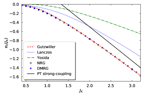
Figure 10: (Color online) Ground-state energy of the one-dimensional symmetric single-impurity Kondo model as a function of the Kondo coupling for intermediate and large couplings, $0.4\leq J_{\rm K}\leq 3.2$. We compare results from strong-coupling perturbation theory (black full line), eq. (42), Gutzwiller theory (red dashed line), first-order Lanczos approximation (blue dotted line), eq. (50), Yosida theory (green dot-dashed line), eq. (58), and numerical data from DMRG (blue crosses) and NRG (black circles).

IX.1.3 Local spin correlation

In Fig. 11 we show the local spin correlation function $C_{0}^{S}(J_{\rm K})$ as a function of the Kondo coupling $J_{\rm K}$. It is zero at $J_{\rm K}=0$ and decreases linearly for small interactions, $C_{0}^{S}(J_{\rm K}\ll 1)=-3J_{\rm K}/16$, see eq. (35). For large interactions, it reaches its limiting value, $C_{0}^{S}(J_{\rm K}\gg 1)=-3/4$, see eq. (43), which corresponds to a singlet formed by the impurity spin and a localized host electron. The DMRG and NRG data give the local spin correlation for all interaction strengths, and faithfully interpolate between the two limiting cases. We verified numerically that the Hellmann-Feynman theorem (12) is fulfilled both in DMRG and NRG.

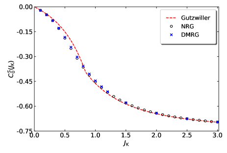
Figure 11: (Color online) Local spin correlation function $C_{0}^{S}(J_{\rm K})$ of the one-dimensional symmetric single-impurity Kondo model as a function of the Kondo coupling $J_{\rm K}$. We compare results from Gutzwiller theory (red dashed line), eq. (87), and numerical data from DMRG (blue crosses) and NRG (black circles). The linear behavior for small couplings, $C_{0}^{S}=-3J_{\rm K}/16$ is given by eq. (35), the limiting value for strong couplings, $C_{0}^{S}(J_{\rm K}\to\infty)=-3/4$ is found from eq. (43).

While the Yosida and first-order Lanczos states are insufficient and thus omitted from the figure, the Gutzwiller wave function reproduces the numerical data for all interactions. The Gutzwiller state with $m>0$ for $J<J_{\rm K,c}^{\rm G}\approx 0.839$ provides a quantitatively satisfactory value for the local spin correlation function but fails qualitatively because the exact solution does not sustain a locally symmetry-broken state. For $J>J_{\rm K,c}^{\rm G}$, the Gutzwiller state very well approximates the local spin correlation function. As seen in Fig. 11, the Gutzwiller, DMRG, NRG results lie almost on top of each other for large Kondo couplings. Therefore, we argue that the strong-coupling expression (95) is actually exact up to and including third order in $1/J_{\rm K}$.

IX.2 Magnetic susceptibilities for weak coupling

For the zero-field susceptibilities only the NRG is capable to examine the weak-coupling limit, $J_{\rm K}\ll 1$, with the desired high accuracy. We mostly investigate the case of a constant density of states, $\rho_{0}^{\rm const}(0)=1/2$, for which the correction term $A_{\Lambda}(\Lambda)$ in eq. (145) was originally derived. Krishna-murthy et al. (1980a, b) For a one-dimensional density of states, we show numerically that the ratio of the impurity-induced susceptibilities is given by the regularized first negative moment of the density of states (60).

IX.2.1 Impurity-induced magnetic susceptibility

In Fig. 12 we show the zero-field impurity-induced magnetic susceptibility as a function of $J_{\rm K}$ for various values of the Wilson parameter $\Lambda$ for a constant density of states, both for a global magnetic field and a local magnetic field at the impurity. The data for $\Lambda=1$ are the result of a quadratic fit in $(\Lambda-1)$ for given $J_{\rm K}$. We plot the ratio of the susceptibilities and the universal part $\bar{\chi}_{0}(j)$, see eq. (122), to focus on the sub-leading terms. The NRG confirms the quadratic dependence of these terms on $j=\rho_{0}(0)J_{\rm K}$ for $J_{\rm K}\to 0$,

$$\frac{\chi_{0}^{\rm ii}(J_{\rm K})}{\bar{\chi}_{0}(j)}=s_{0}+s_{1}j+s_{2}j^{2}+\ldots\;,\quad j=\rho_{0}(0)J_{\rm K}\;.$$ (147)

We collect the results for $s_{0},s_{1},s_{2}$ in table 1.

	$s_{0}$	$s_{1}$	$s_{2}$	$s_{0}$	$\alpha$
$\hat{H}_{\rm m}$A	0.1781(a)	$-$0.401(a)	0.348(a)	0.1784(a)	$-$2.33(a)
	0.1781(b)	$-$0.401(b)	0.348(b)	0.1784(b)	$-$2.35(b)
$\hat{H}_{\rm m,loc}$	0.1734(a)	$-$0.269(a)	0.182(a)	0.1731(a)	$-$1.547(a)
	0.1734(b)	$-$0.269(b)	0.182(b)	0.1731(b)	$-$1.560(b)
exact	0.171099			0.171099

Table 1: Coefficients of the sub-leading terms in the zero-field impurity-induced magnetic susceptibility for the ground state of the symmetric Kondo model with a constant density of states in eq. (147) from NRG, see Fig. 12. The two values result from the two sequences of extrapolations (a) and (b) in $(\Lambda-1)$ and $j$, see text. The analytic value for $s_{0}$ is given in eq. (122). Also given are the coefficients for the fit in eq. (149).

We perform two sequences of extrapolations. In extrapolation (a), we start with a second-order polynomial fit in $(\Lambda-1)$ at fixed $J_{\rm K}$ and fit the resulting data in a second-order polynomial fit in $j=J_{\rm K}\rho_{0}(0)$, as shown in Fig. 12. In extrapolation (b) we first extrapolate in $j$ to determine $s_{l}(\Lambda)$ and extrapolate these coefficients in $\Lambda$ afterwards. NRG data for $0.15\leq J_{\rm K}\leq 1.0$ and $1.8\leq\Lambda\leq 3.2$ are included in the fit. As seen from the data in table 1, the results agree very well.

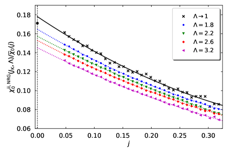
Figure 12: (Color online) Impurity-induced magnetic susceptibility $\chi_{0}^{\rm ii,NRG}(J_{\rm K},\Lambda)$ for a global magnetic field (upper figure) and $\chi_{0,{\rm loc}}^{\rm ii,NRG}(J_{\rm K},\Lambda)$ for a local magnetic field (lower figure) for the symmetric Kondo model with a constant density of states as a function $j=J_{\rm K}\rho_{0}(0)=J_{\rm K}/2$ for various values of the Wilson parameter $\Lambda$. The lines represent the result of a second-order polynomial fit in $j$. To make the sub-leading terms discernible, we scale the susceptibilities by the universal part $\bar{\chi}_{0}(j)$, see eq. (122). The filled symbols at $j=0$ denote the analytical result (122).

The parameter $s_{1}$ is related to Wilson’s coefficients $\alpha_{1}$ and $c_{1}$ in eq. (113) via

$$s_{1}=-\frac{c_{1}/c_{0}+\alpha_{1}}{2{\cal D}\sqrt{\pi e}}\;,\quad\frac{c_{1}}{c_{0}}=-2{\cal D}\sqrt{\pi e}s_{1}-\alpha_{1}\;,$$ (148)

or $c_{1}\approx 0.45$, where we used $C=1$ for a constant density of states, ${\cal D}=1$, $s_{0}\approx-0.40$, $\alpha_{1}\approx 1.5824$, Wilson (1975) and $c_{0}\approx 0.6001$ from eq. (116). Since $|c_{1}/c_{0}|\lesssim\alpha_{1}$, we could also have used

$$\frac{\chi_{0}^{\rm ii}(J_{\rm K})}{\bar{\chi}_{0}(j)}\approx s_{0}e^{-\alpha j}\;,\quad j=\rho_{0}(0)J_{\rm K}$$ (149)

as our fit function. For completeness, the results for this fitting function are also included in table 1.

The constant term is identical in both cases, $s_{0}^{\rm NRG}\approx s_{0,{\rm loc}}^{\rm NRG}\approx s_{0}=1/(2\sqrt{\pi e})\approx 0.1709914$, where we used the analytic result from eq. (122) for comparison. Since the NRG data for a global field show more scatter, the accuracy of $s_{0}$ is smaller than for a local field, the deviations are 4% for a global field and 1% for a local field. In any case, the accuracy is good enough to see that the prefactors of the first-order and second-order terms are different for global and local magnetic fields, $s_{1}\neq s_{1,{\rm loc}}$ and $s_{2}\neq s_{2,{\rm loc}}$. Different linear terms are also found in the Yosida wave function, compare eqs. (V.3.2) and (73).

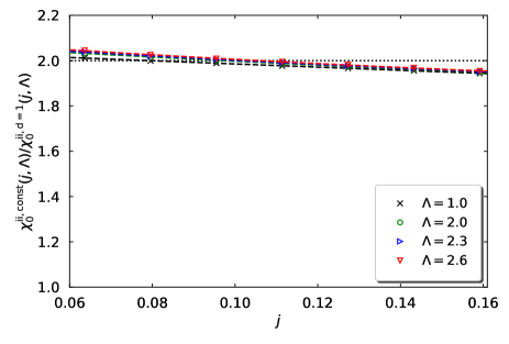
Figure 13: (Color online) Ratio between the zero-field impurity-induced magnetic susceptibility for a constant density of states, $\chi_{0}^{\rm ii,NRG,const}(J_{\rm K},\Lambda)$, and for a one-dimensional density of states, $\chi_{0}^{\rm ii,NRG,d=1}(J_{\rm K},\Lambda)$ for a global magnetic field as a function $j=J_{\rm K}\rho_{0}(0)$ for various values of the Wilson parameter $\Lambda$. The black crosses represent the result of a second-order polynomial fit in $\Lambda-1$. The line $C=2$ gives the result for $j=0$.

IX.2.2 Impurity-induced magnetic susceptibility for a one-dimensional density of states

In Fig. 13 we show the ratio between the zero-field impurity-induced magnetic susceptibility for a constant density of states, $\chi_{0}^{\rm ii,NRG,const}(J_{\rm K},\Lambda)$, and for a one-dimensional density of states, $\chi_{0}^{\rm ii,NRG,d=1}(J_{\rm K},\Lambda)$ for a global magnetic field as a function $j=J_{\rm K}\rho_{0}(0)$ for various values of the Wilson parameter $\Lambda$. The extrapolated value for $\Lambda\to 1$ is very close to $C=2$ which is the exact result for $j=0$, see eq. (122).

Apparently, the result holds for all $j\ll 1$, within the accuracy of the NRG calculations. This universality is also seen in the Yosida wave function, see eq. (V.3.2), where the sub-leading corrections are independent of the host-electron density of states. Therefore, we conjecture that the algebraic correction terms in eq. (122) are universal in the sense that $s_{1}/s_{0}\approx-2.3$ and $s_{2}/s_{0}\approx 2$ do not depend on the form of the host-electron density of states.

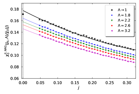
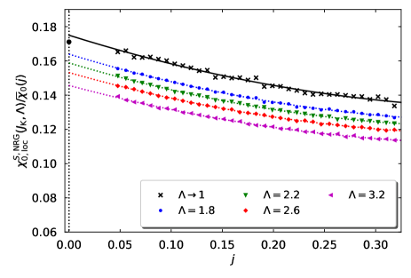
Figure 14: (Color online) Zero-field impurity spin susceptibility $\chi_{0}^{S,{\rm NRG}}(J_{\rm K},\Lambda)$ for a global magnetic field (upper figure) and $\chi_{0,{\rm loc}}^{S,{\rm NRG}}(J_{\rm K},\Lambda)$ for a local magnetic field (lower figure) for the symmetric Kondo model with a constant density of states as a function $j=J_{\rm K}\rho_{0}(0)=J_{\rm K}/2$ for various values of the Wilson parameter $\Lambda$. The lines represent the result of a second-order polynomial fit in $j$. As in Fig. 12, we scale the susceptibilities by the universal part $\bar{\chi}_{0}(j)$. The filled symbols at $j=0$ denote the analytical result (122).

IX.2.3 Impurity spin susceptibility

In Fig. 14 we show the zero-field impurity spin susceptibility as a function of $J_{\rm K}$ for various values of the Wilson parameter $\Lambda$ for a constant density of states, both for a global magnetic field and a local magnetic field at the impurity. The data for $\Lambda=1$ are the result of a quadratic fit in $(\Lambda-1)$ for given $J_{\rm K}$. Again, we plot the ratio of the susceptibilities and the universal part $\bar{\chi}_{0}(j)$, see eq. (122), to focus on the sub-leading terms. The NRG confirms the quadratic dependence of these terms on $j=\rho_{0}(0)J_{\rm K}$ for $J_{\rm K}\to 0$,

$$\frac{\chi_{0}^{S}(J_{\rm K})}{\bar{\chi}_{0}(j)}=S_{0}+S_{1}j+S_{2}j^{2}+\ldots\;,\quad j=\rho_{0}(0)J_{\rm K}\;.$$ (150)

We collect the results for $S_{0},S_{1},S_{2}$ in table 2. Note that we use capital letters here to distinguish the coefficients $s_{l}$ for the impurity-induced susceptibility from the coefficients $S_{l}$ for the impurity spin susceptibility. We also include the results from the extrapolation analogous to eq. (149) which provides the coefficient $\alpha^{S}$ from an exponential extrapolation. NRG data for $0.15\leq J_{\rm K}\leq 1.0$ and $1.8\leq\Lambda\leq 3.2$ are included in the fit.

	$S_{0}$	$S_{1}$	$S_{2}$	$S_{0}$	$\alpha^{S}$A
$\hat{H}_{\rm m}$A	0.1774(a)	$-$0.307(a)	0.300(a)	0.1738(a)	$-$1.49(a)
	0.1774(b)	$-$0.307(b)	0.300(b)	0.1738(b)	$-$1.50(b)
$\hat{H}_{\rm m,loc}$	0.1753(a)	$-$0.193(a)	0.218(a)	0.1707(a)	$-$0.766(a)
	0.1753(b)	$-$0.193(b)	0.218(b)	0.1707(b)	$-$0.766(b)
exact	0.171099			0.171099

Table 2: Coefficients of the sub-leading terms in the zero-field impurity spin susceptibility for the ground state of the symmetric Kondo model with a constant density of states in eq. (147) from NRG, see Fig. 14. The two values result from the two sequences of extrapolations (a) and (b) in $(\Lambda-1)$ and $j$, see text. The analytic value for $S_{0}=s_{0}$ is given in eq. (122). Also given are the coefficients for the fit in eq. (149).

For the impurity spin susceptibility we also find the expected result $S_{0}=s_{0}=1/(2\sqrt{\pi e})\approx 0.1709914$, irrespective of a global or a local field, with deviations of about 4%. Again, the first-order and second-order coefficients $S_{1}$ and $S_{2}$ depend on whether the magnetic field is applied globally or locally.

To assess the accuracy of our extrapolations, we compare the results for $\chi_{0}^{S}(J_{\rm K})$ and $\chi_{0,{\rm loc}}^{\rm ii}(J_{\rm K})$ which should be equal, see eq. (24). We see that $s_{1,{\rm loc}}=-0.269$ agrees reasonably well with $S_{1}=-0.307$, with a deviation of the order of ten percent. However, $s_{2,{\rm loc}}=0.182$ and $S_{2}=0.300$ are off by more than 40 percent. Since the data for the local susceptibilities are better than those for the global susceptibilities, we argue that the data for $s_{1,{\rm loc}}$ and $s_{2,{\rm loc}}$ are more reliable. Nevertheless, the comparison indicates that the values for $s_{1}$ and $S_{1}$ ($s_{2}$ and $S_{2}$) have an uncertainty of several (ten) percent.

IX.3 Magnetic susceptibilities for strong coupling

IX.3.1 Impurity-induced susceptibility

In Fig. 15 we show the zero-field impurity-induced susceptibility with a global and a local field for $J_{\rm K}\geq 1$ from NRG in comparison with the Gutzwiller result. In general, we calculate the impurity-induced magnetization for small local fields and determine the susceptibility from the slope. In the strong-coupling region, this procedure becomes unstable in NRG so that we determine the susceptibility from the second-derivative of the ground-state energy with respect to the global field, see eq. (21).

Figure 15: (Color online) Zero-field impurity-induced susceptibilities $\chi_{0}^{\rm ii}(J_{\rm K})$ and $\chi_{0,{\rm loc}}^{\rm ii}(J_{\rm K})$ on a logarithmic scale for a global and a local magnetic field for the one-dimensional symmetric Kondo model as a function of $J_{\rm K}$ for $J_{\rm K}\geq 1$ from NRG and the Gutzwiller wave function.

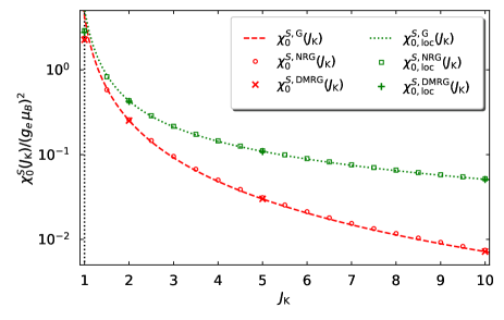
Figure 16: (Color online) Zero-field impurity spin susceptibilities $\chi_{0}^{S}(J_{\rm K})$ and $\chi_{0,{\rm loc}}^{S}(J_{\rm K})$ on a logarithmic scale for a global and a local magnetic field for the one-dimensional symmetric Kondo model as a function of $J_{\rm K}$ for $J_{\rm K}\geq 1$ from NRG, DMRG, and the Gutzwiller wave function.

As seen from Fig. 15, the Gutzwiller wave function almost perfectly reproduces the NRG data for $J_{\rm K}\gtrsim 1.5$. For intermediate to strong couplings, the Gutzwiller wave function is an excellent trial state for the Kondo model.

The strong-coupling asymptotics is shown in Fig. 2. The asymptotic formulae (103) and (104) are applicable for $J_{\rm K}\gtrsim 4$.

IX.3.2 Impurity spin susceptibility

In Fig. 16 we show the zero-field impurity spin susceptibility for $J_{\rm K}\geq 1$. For intermediate to strong couplings, we find an excellent agreement between the data from NRG and DMRG both in the presence of global and local magnetic fields. Again, the Gutzwiller wave function provides an excellent analytic estimate for the zero-field susceptibilities for all $J_{\rm K}\gtrsim 1.5$.

The strong-coupling asymptotics is shown in Fig. 2. The limiting expressions, eqs. (101) and (102), become applicable for $J_{\rm K}\gtrsim 4$.

IX.4 Impurity-induced magnetization and impurity spin polarization for weak coupling

Next, we address the impurity-induced magnetization and the impurity spin polarization as a function of the external field for weak coupling. The comparison of Bethe Ansatz results and NRG data was done only recently. Höck and Schnack (2013)

IX.4.1 Impurity-induced magnetization

Figure 17: (Color online) Impurity-induced magnetization $m^{\rm ii}(B)/(g_{e}\mu_{\rm B})$ for $J_{\rm K}=0.5$ for the one-dimensional symmetric Kondo model as a function of global/local magnetic fields $B$ from the Yosida wave function, NRG, and the Bethe Ansatz.

In Fig. 17 we show the impurity-induced magnetization $m^{\rm ii}(B)/(g_{e}\mu_{\rm B})$ for $J_{\rm K}=0.5$ as a function of the global field $B\leq 0.014$ as obtained from the Yosida wave function, in comparison with NRG data and results from the Bethe Ansatz. We omit the Gutzwiller results because Gutzwiller theory predicts a finite magnetization even at $B=0^{+}$ and thus fails to reproduce the paramagnetic phase at $J_{\rm K}=0.5$. As discussed in Sect. VIII.1, DMRG cannot faithfully reproduce the magnetization for $J_{\rm K}=0.5$ because the tractable system sizes are too small. Therefore, we do not show DMRG data for the impurity-induced magnetization in Fig. 17.

At $J_{\rm K}=0.5$ and in one dimension where $\rho_{0}(0)=1/\pi$, we have $j=\rho_{0}(0)J_{\rm K}=1/(2\pi)\approx 0.159$. The zero-field susceptibility is quite large already. In units of $(g_{e}\mu_{\rm B})^{2}$ we have $\chi_{0}^{\rm ii}(j=1/(2\pi))\approx\bar{\chi}_{0}(1/(2\pi))s_{0}[1+(s_{1}/s_{0})(2\pi)+(s_{2}/s_{0})(2\pi)^{2}]\approx 79$, see eq. (122), where we employ $s_{0}=1/(2{\cal D}C\sqrt{\pi e})\approx 0.0856$ for $C^{d=1}=2$ and ${\cal D}=1$, and make the assumption that the ratios $s_{1}/s_{0}\approx-2.3$ and $s_{2}/s_{0}\approx 2$ do not depend on the host-electron density of states, and are thus obtained from the values in table 1. A large zero-field susceptibility implies a sharp increase of the magnetization for small fields as seen in Fig. 17. The Yosida state overestimates the zero-field susceptibility by more than a factor of five, $\chi_{0}^{\rm ii,Y}(j=1/(2\pi))\approx 433$, see eq. (V.3.2). Thus, the Yosida wave function also overestimates the magnetization for small and intermediate fields, see Fig. 17.

In the Bethe Ansatz, the sharp increase at small fields is followed by a very slow convergence to the limiting value $m^{\rm ii}(B\gg T_{\rm H})=1/2$. The resulting broad magnetization plateau originates from the logarithmic terms in the Bethe Ansatz solution, see eq. (VI-86) in the supplemental material. The NRG results lie on top of the Bethe Ansatz data which shows that the Bethe Ansatz expressions (LABEL:eq:hsmallerthanunity) and (125) remain valid up to $J_{\rm K}$ of the order of a quarter of the bandwidth, as long as $T_{1}$ is determined from the exact zero-field susceptibility from eq. (126).

In Fig. 17 we also show the impurity-induced magnetization $m_{\rm loc}^{\rm ii}(B)$ as a function of a local magnetic field for $J_{\rm K}=0.5$. For small values of the Kondo coupling, the differences between globally and locally applied external fields are fairly small. The impurity-induced magnetization in the presence of a local field is a few percent larger than in the presence of a global field. This can be deduced from eq. (147) which shows that the ratio of the zero-field susceptibilities is close to unity, $[1+(s_{1,{\rm loc}}/s_{0})j+(s_{2,{\rm loc}}/s_{0})j^{2}]/[1+(s_{1}/s_{0})j+(s_{2}/s_{0})j^{2}]\approx 1.13$ at $j=1/(2\pi)$ where the data are taken from table 1. Likewise, the differences between the impurity-induced magnetization $m^{\rm ii}(B)$ and the impurity spin polarization $m^{S}(B)$ are small at small $J_{\rm K}$, $[1+(S_{1}/s_{0})j+(S_{2}/s_{0})j^{2}]/[1+(s_{1}/s_{0})j+(s_{2}/s_{0})j^{2}]\approx 1.12$ at $j=1/(2\pi)$, where the data are taken from table 1 and table 2. This has been noted previously in Ref. [Höck and Schnack, 2013].

In the Yosida wave function, the differences between the impurity-induced magnetization for global and local fields are more pronounced. In the case of a local field, the impurity-induced magnetization in the Yosida wave function quickly reaches the maximal value of one half. For a global field, the impurity-induced magnetization saturates below this value, in contrast to the exact solution. Altogether, the Yosida wave function correctly describes some gross aspects of the magnetization curves (large zero-field susceptibility, monotonous increase to saturation) but it fails to reproduce them in detail, e.g., the small difference between global and local fields.

IX.4.2 Impurity spin polarization

In Fig. 18 we show the impurity spin polarization in the presence of a global and a local field, respectively. As seen from the previous section IX.4.1, the NRG is the best method to study magnetic properties of the Kondo model at weak coupling. Therefore, its results can be used to assess the quality of all other methods.

In Fig. 18 we leave out the Gutzwiller results because the spin polarization is finite at $J_{\rm K}=0.5$, and almost independent of $B$ for all $0\leq B<0.014$, in contrast to the NRG data. The Yosida wave function provides qualitatively correct results but grossly underestimates the spin polarization in both cases. Therefore, the Yosida wave function neither provides an acceptable description of the impurity spin polarization.

Figure 18: (Color online) Impurity spin polarization $S^{z}(B)=m^{S}(B)/(g_{e}\mu_{\rm B})$ as a function of a global magnetic field (upper figure) and $S_{\rm loc}^{z}(B)=m^{S}_{\rm loc}(B)/(g_{e}\mu_{\rm B})$ as a function of a local magnetic field (lower figure) for the one-dimensional symmetric Kondo model at $J_{\rm K}=0.5$ from NRG, DMRG, and the Yosida wave function.

As discussed in Sect. VIII.1, DMRG requires very large system sizes for small Kondo couplings to calculate the impurity spin polarization in the presence of a small global field. Therefore, at $J_{\rm K}=0.5$ the DMRG and NRG data agree only for $B\gtrsim 0.01$ For smaller $B$-values, DMRG substantially overestimates the magnetization, displaying large finite-size effects. Recall that DMRG works for fixed total spin $S^{z}_{\rm tot}$ so that only specific values for $B$ are accessible. This limitation does not apply for a purely local field. It can be tuned freely also in DMRG so that a finite-size extrapolation of the DMRG data for the impurity spin polarization is unproblematic. As seen from Fig. 18, the NRG and DMRG data perfectly agree for the impurity spin polarization in the presence of a local magnetic field. Alternatively, since $m^{S}_{\rm loc}$ is a thermodynamic quantity, it can also be obtained from the derivative of the excess ground-state energy with respect to the external field, see eq. (22). Both approaches lead to the same results.

IX.5 Impurity-induced magnetization and impurity spin polarization for strong coupling

Lastly, we address the impurity-induced magnetization and the impurity spin polarization as a function of the external field for strong coupling.

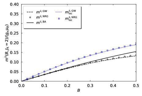
Figure 19: (Color online) Impurity-induced magnetization $m^{\rm ii}(B)/(g_{e}\mu_{\rm B})$ for $J_{\rm K}=2$ for the one-dimensional symmetric Kondo model as a function of a global/local magnetic field $B$ from Bethe Ansatz, NRG, and the Gutzwiller wave function.

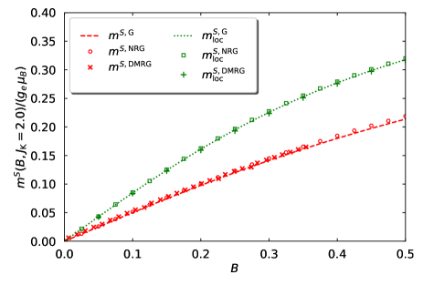
Figure 20: (Color online) Impurity spin polarization $S^{z}(B)=m^{S}(B)/(g_{e}\mu_{\rm B})$ for $J_{\rm K}=2$ for the one-dimensional symmetric Kondo model as a function of a global/local magnetic field $B$ from NRG, DMRG, and the Gutzwiller wave function.

IX.5.1 Impurity-induced magnetization

In Fig. 19 we show the impurity-induced magnetization as a function of $B$ at $J_{\rm K}=2$. When the Kondo coupling reaches the band width, the singlet state between the impurity spin and the band electron at the origin is tightly bound so that the susceptibility is small and even a sizable field can barely polarize the singlet. Therefore, the impurity magnetization remains small for $B\leq 0.5$.

The NRG data lie on top of the analytic results from the Gutzwiller wave function. This again shows that the Gutzwiller wave function is an excellent trial state for the Kondo model at large couplings. At $J_{\rm K}=2$, the Bethe Ansatz is no longer applicable, and sizable differences between NRG/Gutzwiller results and Bethe Ansatz predictions become discernible at large $B$, despite the fact that the linear term is fixed to the exact susceptibility. Values $J_{\rm K}\gtrsim W$ are beyond the Bethe Ansatz description.

IX.5.2 Impurity spin polarization

Finally, in Fig. 20 we show the impurity spin polarization as a function of $B$ at $J_{\rm K}=2$. For large Kondo couplings, the finite-size restrictions imposed on DMRG discussed in Sect. VIII.1 are far less severe, and the results for $L=763$ sites for a global field perfectly reproduce the NRG data for $0\leq B<0.5$. The same perfect agreement between DMRG and NRG data is seen for the case of a local field whose value can be chosen freely also for the DMRG calculations.

The analytic results from the Gutzwiller wave function lie on top the the NRG/DMRG data for both a global and a local field. Again, the Gutzwiller wave function is seen to provide an excellent trial state for the Kondo model at large couplings.

X Conclusions

In the last section, we summarize our central findings and discuss our main results.

X.1 Summary

In our work, we investigated the symmetric single-impurity Kondo model on a chain at zero temperature. As a function of the Kondo coupling $J_{\rm K}$, we studied the ground-state energy, the local spin correlation function, the impurity spin polarization and impurity-induced magnetization, and the corresponding zero-field magnetic susceptibilities for global and local external fields $B$. Some of these quantities, e.g., the ground-state energy and the local spin correlation function, are related by the Hellmann-Feynman theorem that also holds for variational wave functions, see appendix B.1.

We calculated the ground-state energy and the local spin correlation function in weak-coupling and strong-coupling perturbation theory at $B=0$ as benchmark for our approaches. Some of the required calculations were deferred to appendix B.2 for weak coupling and to appendix B.3 for strong coupling.

As the first of three analytical variational methods, we analyzed the first-order Lanczos state at $B=0$, as done by Mancini and Mattis Mancini and Mattis (1985) for a constant density of states. We recapitulated the Lanczos method and performed the calculation of the first-order coefficients in appendix B.2. Second, we extended and evaluated the Yosida wave function Yosida (1966, 1996) to include external magnetic fields. The Yosida wave function provides a simple description of the Kondo-singlet ground state with an exponentially small binding energy at small Kondo couplings that translates into an exponentially large zero-field magnetic susceptibility. Third, we introduced and employed the Gutzwiller variational state Gutzwiller (1964); Linneweber et al. (2017) at finite fields. The latter provides a Hartree-Fock type description of the Kondo model that guarantees that the impurity is singly occupied. The Gutzwiller wave function becomes exact in the limit of large Kondo couplings, $J_{\rm K}\gg W$. The evaluation of the Gutzwiller wave function required the solution of the non-interacting single-impurity Anderson model (SIAM) in the presence of potential scattering. This was done in appendix B.4.

As numerical techniques, we employed the Numerical Renormalization Group (NRG) Wilson (1975); Krishna-murthy et al. (1980a, b); Bulla et al. (2008) and the Density-Matrix Renormalization Group (DMRG) White and Noack (1992); White (1992, 1993)methods. Using the DMRG method we addressed finite half-chains of length $L/2$, and performed quadratic fits in $1/L$ for physical quantities to extrapolate to the thermodynamic limit, $L\to\infty$. In DMRG, the system sizes are limited to $L\lesssim 10^{3}$ so that we could not address the impurity-induced magnetizations and the zero-field susceptibilities at weak Kondo couplings. The NRG permits the accurate calculation of all ground-state quantities as a function of the Wilson parameter $\Lambda$. We performed quadratic fits in $(\Lambda-1)$ to extrapolate our data to the limit $\Lambda=1$. We employed the correction factor derived by Krishna-murthy, Wilkins, and Wilson Krishna-murthy et al. (1980a, b) because it improved the quality of the extrapolations.

Since the Bethe Ansatz solves a Kondo model with linear dispersion and infinite bandwidth, a direct comparison of physical quantities is not easy because there is a non-trivial relation between the Kondo couplings $J_{\rm K}^{\rm BA}$ and $J_{\rm K}$ used in the Bethe Ansatz and in the lattice model, respectively. As we showed in appendix B.5, the ground-state energy in the Bethe Ansatz is zero, up to corrections of the order $(J_{\rm K}^{\rm BA})^{3}$. Thus, the ground-state energy from Bethe Ansatz cannot be used for a comparison with the lattice model. Using known results from Andrei, Furuya, and Lowenstein, Andrei et al. (1983) re-derived in appendix B.6 and extended to a general host-electron density of states, we expressed $J_{\rm K}^{\rm BA}$ as a series expansion in $J_{\rm K}$, and gave analytic expressions for the leading-order terms in eq. (123).

When the zero-field susceptibility from NRG is used, the impurity-induced magnetization from Bethe Ansatz and from NRG were seen to agree perfectly. This was observed earlier in the NRG analysis of Schnack and Höck. Höck and Schnack (2013)

In our work, we showed that the various zero-field susceptibilities have a universal small-coupling limit, see eq. (122). For finite $J_{\rm K}$, however, the impurity spin polarization and the impurity-induced magnetization at global and local fields differ from each other by a factor that goes to unity for $J_{\rm K}\to 0$. Using NRG, we calculated the corrections numerically, with an accuracy of some ten percent. Since two zero-field susceptibilities agree, see eq. (24), it is possible to assess the accuracy of the NRG calculations for the zero-field susceptibilities.

X.2 Discussion

The ground state of the symmetric single-impurity Kondo model describes a Kondo singlet formed by the impurity spin and its host-electron screening cloud. Unfortunately, it is by no means easy to formulate a concise, analytically tractable variational wave function that adequately describes the ground state for all couplings.

In this work we showed that the Gutzwiller wave function provides an excellent trial state for large Kondo couplings, $J_{\rm K}\gtrsim W$, where $W=2$ is the bandwidth. It reproduce the ground-state energy, the local spin correlation, the impurity spin polarization and impurity-induced magnetization, and the corresponding zero-field susceptibilities from NRG and DMRG with high accuracy. Unfortunately, it displays a Hartree-Fock type transition to a state with an oriented impurity spin below $J_{\rm K,c}^{\rm G}\approx 0.893$ that is not contained in the exact solution of the model.

For weak coupling, the Yosida wave function reproduces the exponential divergence of the zero-field susceptibilities known from Bethe Ansatz and NRG but it fails to provide a good variational bound on the ground-state energy for all couplings. Eventually, it becomes unstable for large Kondo couplings. Thus, the Yosida and Gutzwiller variational approaches provide a complementary view on the Kondo-singlet ground state of the Kondo model.

The DMRG method numerically determines an optimal variational ground state for the Kondo model on finite lattices. Although not specifically designed for impurity models, the method works very well as long as all energy scales lie within the DMRG energy resolution $\Delta\epsilon=W/L$. However, the Kondo temperature in the Kondo model becomes exponentially small for $J_{\rm K}\ll W$ so that the calculation of magnetic properties using DMRG is limited to $J_{\rm K}\gtrsim 0.5$ for the one-dimensional density of states. Other quantities such as the ground-state energy and the local spin correlation function are unproblematic. For $J_{\rm K}=2$, the results from NRG and DMRG agree perfectly, not only for the ground-state energy and local spin correlation but also for the impurity spin polarization and zero-field susceptibility. The DMRG can also be applied to impurity problems as long as all intrinsic energy scales can be resolved appropriately.

The NRG was specifically designed to treat exponentially small energy scales in impurity models and thus works exceedingly well for the Kondo model. In this work we showed that NRG also permits the accurate calculation of the ground-state energy and local spin correlation function. In particular, we found that an extrapolation $\Lambda\to 1$ is required whereby the correction factor derived by Krishna-murthy, Wilkins, and Wilson Krishna-murthy et al. (1980a, b) is helpful to improve the extrapolations.

In contrast to the single-impurity Anderson model, Barcza et al. (2019) the Bethe Ansatz results for the Kondo model cannot be directly compared to numerical results because the continuum and lattice models differ in their coupling constants. Therefore, at zero temperature, only the impurity-induced magnetization for small Kondo couplings can eventually be compared to the NRG data. For this reason, it was indispensable to generate accurate data from NRG for comparison with the analytical and numerical variational methods (Lanczos, Yosida, Gutzwiller, DMRG) employed in this work.

Appendix A Technical details

A.1 Diagonalization of the kinetic energy operator

We use open boundary conditions and define the operators for standing waves,

$$\hat{a}_{k,\sigma}^{\vphantom{+}}=\sqrt{\frac{2}{L+1}}\sum_{n=-(L-1)/2}^{(L-1)/2}\sin\Bigl{(}\frac{\pi kn}{L+1}+\frac{\pi k}{2}\Bigr{)}\hat{c}_{n,\sigma}^{\vphantom{+}}\;.$$ (151)

We may formally include the operators $\hat{c}_{\pm(L+1)/2,\sigma}$ at sites $n=\pm(L+1)/2$ because they do not enter the standing-wave operators $\hat{a}_{k,\sigma}$. The inverse transformation reads

$$\hat{c}_{n,\sigma}^{\vphantom{+}}=\sqrt{\frac{2}{L+1}}\sum_{k=1}^{L}\sin\left[\frac{\pi k}{L+1}\left(n+\frac{L+1}{2}\right)\right]\hat{a}_{k,\sigma}^{\vphantom{+}}\;.$$ (152)

The kinetic energy becomes diagonal

$$\hat{T}=\sum_{k=1,\sigma}^{L}\epsilon_{k}\hat{a}_{k,\sigma}^{+}\hat{a}_{k,\sigma}^{\vphantom{+}}$$ (153)

with the dispersion relation ($1\leq k\leq L$)

$$\epsilon_{k}=-2t\cos\left(\frac{\pi k}{L+1}\right)\;.$$ (154)

A.2 Half-chain geometry

Eq. (152) shows that

$$\hat{c}_{0,\sigma}=\sqrt{\frac{2}{L+1}}\sum_{k=1}^{L}\sin\left[\frac{\pi k}{2}\right]\hat{a}_{k,\sigma}^{\vphantom{+}}\;.$$ (155)

Therefore, the standing waves with even $k$ do not couple to the chain center, and drop out of the problem.

A.2.1 Canonical transformation to parity eigenstates

The reason for this decoupling is parity symmetry. To make it transparent in the real-space representation, we introduce the operators for $n=1,2,\ldots,(L-1)/2$

$$\hat{C}_{n,\sigma}^{\vphantom{+}} = \sqrt{\frac{1}{2}}\left(\hat{c}_{n,\sigma}^{\vphantom{+}}+\hat{c}_{-n,\sigma}^{\vphantom{+}}\right)\;,$$

$$\hat{S}_{n,\sigma}^{\vphantom{+}} = \sqrt{\frac{1}{2}}\left(\hat{c}_{n,\sigma}^{\vphantom{+}}-\hat{c}_{-n,\sigma}^{\vphantom{+}}\right)\;,$$ (156)

with the inverse transformation

$$\hat{c}_{n,\sigma}^{\vphantom{+}} = \sqrt{\frac{1}{2}}\left(\hat{C}_{n,\sigma}^{\vphantom{+}}+\hat{S}_{n,\sigma}^{\vphantom{+}}\right)\;,$$

$$\hat{c}_{-n,\sigma}^{\vphantom{+}} = \sqrt{\frac{1}{2}}\left(\hat{C}_{n,\sigma}^{\vphantom{+}}-\hat{S}_{n,\sigma}^{\vphantom{+}}\right)\;.$$ (157)

Moreover, we set $\hat{C}_{0,\sigma}^{\vphantom{+}}\equiv\hat{c}_{0,\sigma}^{\vphantom{+}}$ for notational consistency. The transformation is a canonical basis transformation.

Then, the kinetic energy becomes

$$\hat{T} = -t\left[\sqrt{2}\hat{C}_{0,\sigma}^{+}\hat{C}_{1,\sigma}^{\vphantom{+}}+\hbox{h.c.}\right]$$ (158)

$$-t\biggl{[}\frac{1}{2}\sum_{n=1,\sigma}^{(L-3)/2}\left(\hat{C}_{n+1,\sigma}^{+}+\hat{S}_{n+1,\sigma}^{+}\right)\left(\hat{C}_{n,\sigma}^{\vphantom{+}}+\hat{S}_{n,\sigma}^{\vphantom{+}}\right)$$

$$\hphantom{-t\biggl{[}}+\frac{1}{2}\sum_{n=1,\sigma}^{(L-3)/2}\left(\hat{C}_{n+1,\sigma}^{+}-\hat{S}_{n+1,\sigma}^{+}\right)\left(\hat{C}_{n,\sigma}^{\vphantom{+}}-\hat{S}_{n,\sigma}^{\vphantom{+}}\right)$$

$$\hphantom{-t\biggl{[}}+\hbox{h.c.}\biggr{]}$$

$$\equiv \hat{T}^{C}+\hat{T}^{S}\;,$$

where the two commuting parts of the kinetic energy are given by

$$\hat{T}^{C} = -\sqrt{2}t\sum_{\sigma}\left(\hat{C}_{0,\sigma}^{+}\hat{C}_{1,\sigma}^{\vphantom{+}}+\hat{C}_{1,\sigma}^{+}\hat{C}_{0,\sigma}^{\vphantom{+}}\right)$$

$$+(-t)\sum_{n=1,\sigma}^{(L-3)/2}\left(\hat{C}_{n+1,\sigma}^{+}\hat{C}_{n,\sigma}^{\vphantom{+}}+\hat{C}_{n,\sigma}^{+}\hat{C}_{n+1,\sigma}^{\vphantom{+}}\right)\,,$$

$$\hat{T}^{S} = (-t)\sum_{n=1,\sigma}^{(L-3)/2}\left(\hat{S}_{n+1,\sigma}^{+}\hat{S}_{n,\sigma}^{\vphantom{+}}+\hat{S}_{n,\sigma}^{+}\hat{S}_{n+1,\sigma}^{\vphantom{+}}\right)\;.$$ (159)

Therefore, the $S$-electrons drop out of the problem, and the Kondo Hamiltonian reduces to

$$\hat{H}_{\rm K}^{C}=\hat{T}^{C}+\hat{V}_{\rm sd}+\hat{H}_{\text{m}}$$ (160)

with

$$\hat{V}_{\rm sd} = \frac{J_{\rm K}}{2}\left(\hat{C}_{0,\uparrow}^{+}\hat{C}_{0,\downarrow}^{\vphantom{+}}\hat{d}_{\downarrow}^{+}\hat{d}_{\uparrow}^{\vphantom{+}}+\hat{C}_{0,\downarrow}^{+}\hat{C}_{0,\uparrow}^{\vphantom{+}}\hat{d}_{\uparrow}^{+}\hat{d}_{\downarrow}^{\vphantom{+}}\right)$$

$$+\frac{J_{\rm K}}{4}\left(\hat{d}_{\uparrow}^{+}\hat{d}_{\uparrow}^{\vphantom{+}}-\hat{d}_{\downarrow}^{+}\hat{d}_{\downarrow}^{\vphantom{+}}\right)\left(\hat{C}_{0,\uparrow}^{+}\hat{C}_{0,\uparrow}^{\vphantom{+}}-\hat{C}_{0,\downarrow}^{+}\hat{C}_{0,\downarrow}^{\vphantom{+}}\right)\;,$$

$$\hat{H}_{\text{m}} = \hat{H}_{\text{m},\text{loc}}-B\sum_{n=0}^{(L-1)/2}\Bigl{[}\hat{C}_{n,\uparrow}^{+}\hat{C}_{n,\uparrow}^{\vphantom{+}}-\hat{C}_{n,\downarrow}^{+}\hat{C}_{n,\downarrow}^{\vphantom{+}}\Bigr{]}$$ (161)

and $\hat{H}_{\text{m},\text{loc}}=-B(\hat{d}_{\uparrow}^{+}\hat{d}_{\uparrow}^{\vphantom{+}}-\hat{d}_{\downarrow}^{+}\hat{d}_{\downarrow}^{\vphantom{+}})$. Note that the $C$-parity eigenbasis in this one-dimensional finite-size chain takes on the role of the $s$-wave scattering in the three-dimensional continuous model, Wilson (1975) where all other spherical harmonics drop out of the problem. Now, the impurity is at the left end of the half-chain. The half-chain has an odd number of sites, $L_{\rm hc}=(L+1)/2$, so that the system of half-chain plus impurity has a total number of even sites because we choose $(L+3)/2$ to be even. In the absence of an external magnetic field, we have an equal number of electrons with spin $\sigma=\uparrow,\downarrow$ in the half-chain, $N_{\sigma}=(L+3)/4$, so that the ground state has total spin zero.

A.2.2 Kinetic energy of the half-chain

We denote for $m=1,\ldots,(L+1)/2$

$$\hat{b}_{m,\sigma}^{\vphantom{+}} \equiv (-1)^{m-1}\hat{a}_{2m-1,\sigma}^{\vphantom{+}}\;,$$

$$\epsilon(m) = -2t\cos\left[\frac{\pi(2m-1)}{L+1}\right]$$ (162)

and find

$$\hat{T}^{C}=\sum_{m=1,\sigma}^{(L+1)/2}\epsilon(m)\hat{b}_{m,\sigma}^{+}\hat{b}_{m,\sigma}^{\vphantom{+}}$$ (163)

for the kinetic energy of the half-chain in diagonal form. For half filling of the half-chain, the Fermi energy is at $E_{\rm F}=0$, i.e., the last occupied site in Fourier space is $m_{\rm F}=(L+3)/4$ with energy $\epsilon(m_{\rm F})=0$.

We rewrite the dispersion relation as

$$\epsilon(m)=2t\sin\left[\frac{2\pi(m-m_{\rm F})}{L+1}\right]\;,$$ (164)

which can be linearized around the Fermi wave number,

$$\epsilon(m)\approx 2t\frac{2\pi(m-m_{\rm F})}{L+1}+{\cal O}\left((m-m_{\rm F})^{3}\right)$$ (165)

for $|m-m_{\rm F}|\ll L$ so that the Fermi velocity becomes

$$v_{\rm F}=\frac{\epsilon(m_{\rm F}+1)-\epsilon(m_{\rm F})}{2\pi/(L+1)}=2t\;.$$ (166)

In Bethe Ansatz calculations, $v_{\rm F}^{\rm BA}\equiv 1$ is used. Therefore, it is convenient to set $2t\equiv 1$ so that the bandwidth is $W=2$.

A.3 Weak-coupling perturbation theory

A.3.1 Perturbation theory to leading order

To leading order, we choose finite system sizes $L$, and consider the full-chain geometry. In Fourier space, the kinetic energy operator and the Kondo coupling for the chain are given by

$$\hat{T} = \sum_{k=1,\sigma}^{L}\epsilon_{k}\hat{a}_{k,\sigma}^{+}\hat{a}_{k,\sigma}^{\vphantom{+}}\;,$$ (167)

$$\hat{V}_{\rm sd} = \frac{J_{\rm K}}{L+1}\sum_{k,p=1}^{L}\sin(\pi k/2)\sin(\pi p/2)$$

$$\times\biggl{(}\hat{d}_{\downarrow}^{+}\hat{d}_{\uparrow}^{\vphantom{+}}\hat{a}_{k,\uparrow}^{+}\hat{a}_{p,\downarrow}^{\vphantom{+}}+\hat{d}_{\uparrow}^{+}\hat{d}_{\downarrow}^{\vphantom{+}}\hat{a}_{k,\downarrow}^{+}\hat{a}_{p,\uparrow}^{\vphantom{+}}$$

$$\quad+\frac{1}{2}\left(\hat{d}_{\uparrow}^{+}\hat{d}_{\uparrow}^{\vphantom{+}}-\hat{d}_{\downarrow}^{+}\hat{d}_{\downarrow}^{\vphantom{+}}\right)\left(\hat{a}_{k,\uparrow}^{+}\hat{a}_{p,\uparrow}^{\vphantom{+}}-\hat{a}_{k,\downarrow}^{+}\hat{a}_{p,\downarrow}^{\vphantom{+}}\right)\biggr{)}\;.$$

Due to spin symmetry we find

$$\langle\Phi_{0}|\hat{T}|\Phi_{0}\rangle=\langle A|\hat{T}|A\rangle=E_{\rm FS}-\epsilon_{k_{\rm F}}=E_{\rm FS}$$ (169)

because $\epsilon_{k_{\rm F}}=0$ . Moreover,

$$\langle\Phi_{0}|\hat{V}_{\rm sd}|\Phi_{0}\rangle = -\frac{3J_{\rm K}}{2(L+1)}\sum_{k,p=1}^{L}\sin(\pi k/2)\sin(\pi p/2)$$ (170)

$$\hphantom{-\frac{3J_{\rm K}}{2(L+1)}\sum_{k,p=1}^{L}}\langle A|\hat{a}_{k,\uparrow}^{+}\hat{a}_{p,\uparrow}^{\vphantom{+}}-\hat{a}_{k,\downarrow}^{+}\hat{a}_{p,\downarrow}^{\vphantom{+}}|A\rangle$$

$$= -\frac{3J_{\rm K}}{2(L+1)}$$

because $\sin^{2}(\pi k_{\rm F}/2)=1$. Thus we obtain

$$e_{0}^{(1)}(J_{\rm K})=E_{0}^{(1)}(J_{\rm K})-E_{\rm FS}=-\frac{3J_{\rm K}}{2}\frac{1}{L+1}\;.$$ (171)

In first order in $J_{\rm K}$, the energy decrease is only of the order $1/L$.

A.3.2 Perturbation theory to second order

To second order, we implicitly work in the thermodynamic limit, $L\to\infty$. The second-order energy correction reads

$$e_{0}^{(2)}(J_{\rm K})=\sum_{|m\rangle\neq|\Phi_{0}\rangle}\frac{\left|\langle m|\hat{V}_{\rm sd}|\Phi_{0}\rangle\right|^{2}}{E_{0}^{(0)}-E_{m}^{(0)}}\;.$$ (172)

All states that can be reached from $|\Phi_{0}\rangle$ by an application of $\hat{V}_{\rm sd}$ have an extra particle in one of the $L/2$ single-particle levels above the Fermi sea at $p>k_{\rm F}$ and a hole in one of the $L/2$ single-particle levels below $k_{\rm F}$, $k\leq k_{\rm F}$, see eq. (A.3.1). Therefore, $E_{0}^{(0)}-E_{k,p}^{(0)}=-(\epsilon_{p}-\epsilon_{k})$. Otherwise, the coupling matrix element is independent of $k$ and $p$. Therefore, in the thermodynamic limit, we may sum over all $(L/2)^{2}$ intermediate states and find

$$e_{0}^{(2)}(J_{\rm K})=-\left(\frac{2}{L}\right)^{2}\sum_{k=1}^{k_{\rm F}}\sum_{p=k_{\rm F}}^{L}\frac{\langle\Phi_{0}|\hat{V}_{\rm sd}^{2}|\Phi_{0}\rangle}{\epsilon_{p}-\epsilon_{k}}\equiv-fb_{1}^{2}$$ (173)

with

$$f = 4\int_{0}^{1}{\rm d}\omega_{1}\int_{-1}^{0}{\rm d}\omega_{2}\rho_{0}(\omega_{1})\rho_{0}(\omega_{2})\frac{1}{\omega_{1}-\omega_{2}}\;,$$ (174)

$$b_{1}^{2} = \langle\Phi_{0}|\hat{V}_{\rm sd}^{2}|\Phi_{0}\rangle\;.$$ (175)

As shown in appendix B.2, we have $b_{1}^{2}=3J_{\rm K}^{2}/32$, independent of the density of states.

For the one-dimensional density of states (8) we find

$$f=\int_{0}^{\infty}{\rm d}\omega e^{-\omega\eta}J_{0}(\omega)\bm{H}_{0}(\omega)\;,$$ (176)

where $\eta=0^{+}$, $J_{0}(\omega)$ is the zeroth order Bessel function and $\bm{H}_{0}(\omega)$ is the zeroth order Struve function, see eqs. (9.1.18) and (12.1.7) of Ref. [Abramowitz and Stegun, 1964]. Using eq. (12.1.19) of Ref. [Abramowitz and Stegun, 1964] this can further be simplified to

$$f=\frac{8}{\pi}\sum_{k=0}^{\infty}\frac{1}{2k+1}\int_{0}^{\infty}{\rm d}\omega J_{0}(\omega)J_{2k+1}(\omega)=1\;,$$ (177)

where we used eq. (6.512,2) of Ref. [Gradshteyn and Ryzhik, 2007]. Thus, our final result to second order is

$$e_{0}^{(2)}(J_{\rm K})=-\frac{3}{32}J_{\rm K}^{2}$$ (178)

for the one-dimensional density of states (8).

A.4 Energy of the magnetic Yosida state

A.4.1 Host electron Fermi sea

At half band-filling and for a symmetric density of states we have

$$|\hbox{FS}\rangle=\prod_{k;\epsilon_{k}\leq-\epsilon_{\rm F}}\hat{a}_{k,\downarrow}^{+}\prod_{k;\epsilon_{k}\leq\epsilon_{\rm F}}\hat{a}_{k,\uparrow}^{+}|\hbox{vac}\rangle\;.$$ (179)

The host-electron spin polarization per site

$$s_{0}=\frac{1}{2}\frac{1}{L}\sum_{k}\langle\hbox{FS}|\hat{a}_{k,\uparrow}^{+}\hat{a}_{k,\uparrow}^{\vphantom{+}}-\hat{a}_{k,\downarrow}^{+}\hat{a}_{k,\downarrow}^{\vphantom{+}}|\hbox{FS}\rangle$$ (180)

determines $\epsilon_{\rm F}$. For the one-dimensional density of states we find

$$s_{0}=\frac{1}{\pi}\arcsin\epsilon_{\rm F}\quad,\quad\epsilon_{\rm F}=\sin(\pi s_{0})\;.$$ (181)

In turn, $\epsilon_{\rm F}$ can be viewed as a variational parameter that optimizes the ground-state energy in the presence of the external field,

$$e_{\rm FS}(\epsilon_{\rm F}) = t_{\rm FS}(\epsilon_{\rm F})-2Bs_{0}(\epsilon_{\rm F})\;,$$

$$t_{\rm FS}(\epsilon_{\rm F}) = \frac{1}{L}\langle\hbox{FS}|\hat{T}|\hbox{FS}\rangle$$ (182)

$$= 2\int_{-1}^{0}{\rm d}\omega\omega\rho_{0}(\omega)+2\int_{0}^{\epsilon_{\rm F}}{\rm d}\omega\omega\rho_{0}(\omega)\;.$$

For a symmetric density of states at half band-filling, the variational optimum is at

$$\epsilon_{\rm F}^{(0)}=B$$ (183)

for $B\leq 1$ and $\epsilon_{\rm F}^{(0)}=1$ for $B\geq 1$. Thus, in one dimension for $B\leq 1$

$$e_{\rm FS}(B)=-\frac{2}{\pi}\sqrt{1-B^{2}}-\frac{2}{\pi}B\arcsin(B)\;.$$ (184)

A.4.2 Presence of the impurity

In the presence of the impurity, we have to determine $\epsilon_{\rm F}$ from the minimization of

$$E_{0}(\epsilon_{\rm F})=Le_{\rm FS}(\epsilon_{\rm F})+e_{0}(\epsilon_{\rm F})\;.$$ (185)

This gives the condition

$$0=Le_{\rm FS}^{\prime}(\epsilon_{\rm F}^{\rm opt})+e_{0}^{\prime}(\epsilon_{\rm F}^{\rm opt})\;.$$ (186)

We separate the terms of order $L$ and order unity,

$$\epsilon_{\rm F}^{\rm opt}=B+\frac{1}{L}\epsilon_{\rm F}^{(1)}\;,$$ (187)

where we use eq. (183) to identify the leading-order term $\epsilon_{\rm F}^{(0)}=B$, and find in eq. (186) that

$$0 = e_{\rm FS}^{\prime\prime}(B)\epsilon_{\rm F}^{(1)}+e_{0}^{\prime}(B)\;,$$

$$\epsilon_{\rm F}^{(1)} = -\frac{e_{0}^{\prime}(B)}{e_{\rm FS}^{\prime\prime}(B)}=-\frac{1}{2\rho_{0}(B)}\left.\frac{\partial e_{0}(\epsilon_{\rm F})}{\partial\epsilon_{\rm F}}\right|_{\epsilon_{\rm F}=B}\;.$$ (188)

In the last equation we used eq. (182) to show that

$$e_{\rm FS}^{\prime}(\epsilon_{\rm F}) = 2(\epsilon_{\rm F}-B)\rho_{0}(\epsilon_{\rm F})\;,$$

$$e_{\rm FS}^{\prime\prime}(\epsilon_{\rm F}) = 2\rho_{0}(\epsilon_{\rm F})+2(\epsilon_{\rm F}-B)\rho_{0}^{\prime}(\epsilon_{\rm F})\;.$$ (189)

Fortunately, we do not need to know $\epsilon_{\rm F}^{(1)}$ when we work with the ground-state energy because

$$E_{0}(\epsilon_{\rm F}^{\rm opt}) = L\Bigl{(}e_{\rm FS}(B)+e_{\rm FS}^{\prime}(B)\frac{\epsilon_{\rm F}^{(1)}}{L}\Bigr{)}+e_{0}(B)$$ (190)

$$= Le_{\rm FS}(B)+e_{0}(B)$$

is independent of $\epsilon_{\rm F}^{(1)}$ due to eq. (182), see also eq. (189).

A.4.3 Lagrange functional and minimization

After calculating all expectation values, the Lagrange functional for the Yosida state ${\cal L}\equiv{\cal L}\left[\left\{\alpha_{k,\uparrow}\right\},\left\{\alpha_{k,\downarrow}\right\},\lambda\right]$ becomes

$${\cal L} = \frac{1}{2}\left(\frac{1}{L}\mathop{\sum\nolimits^{\prime}}_{k}\alpha_{k,\downarrow}^{2}\epsilon_{k}+\frac{1}{L}\mathop{\sum\nolimits^{\prime\prime}}_{k}\alpha_{k,\uparrow}^{2}\epsilon_{k}\right)$$ (191)

$$-\frac{J_{\rm K}}{2}\left(\frac{1}{L}\mathop{\sum\nolimits^{\prime}}_{k}\alpha_{k,\downarrow}\right)\left(\frac{1}{L}\mathop{\sum\nolimits^{\prime\prime}}_{k}\alpha_{k,\uparrow}\right)$$

$$+\frac{J_{\rm K}}{4}s_{0}\left(\frac{1}{L}\mathop{\sum\nolimits^{\prime}}_{k}\alpha_{k,\downarrow}^{2}-\frac{1}{L}\mathop{\sum\nolimits^{\prime\prime}}_{k}\alpha_{k,\uparrow}^{2}\right)$$

$$-\frac{J_{\rm K}}{8}\left(\frac{1}{L}\mathop{\sum\nolimits^{\prime}}_{k}\alpha_{k,\downarrow}\right)^{2}-\frac{J_{\rm K}}{8}\left(\frac{1}{L}\mathop{\sum\nolimits^{\prime\prime}}_{k}\alpha_{k,\uparrow}\right)^{2}$$

$$+\lambda\left(1-\frac{1}{2L}\mathop{\sum\nolimits^{\prime}}_{k}\alpha_{k,\downarrow}^{2}-\frac{1}{2L}\mathop{\sum\nolimits^{\prime\prime}}_{k}\alpha_{k,\uparrow}^{2}\right)\;,$$

where we took the normalization into account using the Lagrange parameter $\lambda$.

We define

$$C_{\uparrow} = \frac{1}{L}\mathop{\sum\nolimits^{\prime\prime}}_{k}\alpha_{k,\uparrow}\;,$$

$$C_{\downarrow} = \frac{1}{L}\mathop{\sum\nolimits^{\prime}}_{k}\alpha_{k,\downarrow}\;.$$ (192)

The variation of the Lagrange functional (191) gives

$$\alpha_{k,\uparrow} = \frac{J_{\rm K}}{4}\frac{C_{\uparrow}+2C_{\downarrow}}{\epsilon_{k}-(\lambda+J_{\rm K}s_{0}/2)}\;,$$

$$\alpha_{k,\downarrow} = \frac{J_{\rm K}}{4}\frac{C_{\downarrow}+2C_{\uparrow}}{\epsilon_{k}-(\lambda-J_{\rm K}s_{0}/2)}$$ (193)

in the respective regions in $k$-space. We abbreviate the principal-value integral

$$F_{1}(x,B)=\mathchoice{{\vbox{\hbox{$\textstyle-$}}\kern-4.86108pt}}{{\vbox{\hbox{$\scriptstyle-$}}\kern-3.25pt}}{{\vbox{\hbox{$\scriptscriptstyle-$}}\kern-2.29166pt}}{{\vbox{\hbox{$\scriptscriptstyle-$}}\kern-1.875pt}}\!\int_{B}^{1}{\rm d}\omega\rho_{0}(\omega)\frac{1}{\omega-x}$$ (194)

to find in eq. (192)

$$C_{\uparrow} = \frac{J_{\rm K}}{4}\left(C_{\uparrow}+2C_{\downarrow}\right)F_{1}(\lambda+J_{\rm K}s_{0}/2,B)\;,$$

$$C_{\downarrow} = \frac{J_{\rm K}}{4}\left(C_{\downarrow}+2C_{\uparrow}\right)F_{1}(\lambda-J_{\rm K}s_{0}/2,-B)\;,$$ (195)

whereby we assume throughout that $0\leq B<1$, i.e., the host electrons are not fully polarized. Note that eq. (190) permits to set $\epsilon_{\rm F}=B$ in our further considerations.

The secular determinant that belongs to eq. (195) must be zero because the normalization condition $(C_{\uparrow}+C_{\downarrow})/2=1$ must also be fulfilled. Therefore, we determine $\lambda$ from the equation

$$\left(1-\frac{J_{\rm K}F_{+}}{4}\right)\left(1-\frac{J_{\rm K}F_{-}}{4}\right)-\frac{J_{\rm K}^{2}F_{+}F_{-}}{4}=0\;,$$ (196)

where we abbreviated $F_{+}\equiv F_{1}(\lambda+J_{\rm K}s_{0}/2,B)$ and $F_{-}\equiv F_{1}(\lambda-J_{\rm K}s_{0}/2,-B)$. In one spatial dimension we have $s_{0}(B)=(1/\pi)\arcsin(B)$ from eq. (183) and

$$F_{1}(x,B)=\frac{1}{\pi\sqrt{1-x^{2}}}\ln\biggl{[}\frac{1-Bx+\sqrt{(1-B^{2})(1-x^{2})}}{B-x}\biggr{]}.$$ (197)

Using the variationally optimal parameters, it is not difficult to show that

$$e_{0}^{\rm Y}(J_{\rm K},B)=\lambda\;.$$ (198)

Therefore, eq. (196) determines the variational ground-state energy as a function of the external field $B$.

Eq. (196) provides a solution only for $B\leq B_{\rm c}^{\rm Y}(J_{\rm K})$ above which the Yosida state becomes unstable. This problem does not occur in the Gutzwiller description so that we do not extend the Yosida state to the region $B>B_{\rm c}^{\rm Y}(J_{\rm K})$.

A.5 Impurity spin polarization and magnetization of the Yosida state

A.5.1 Impurity spin polarization

By definition, see eq. (14), the impurity spin polarization is given by

$$\frac{m^{S,{\rm Y}}(J_{\rm K},B)}{g_{\rm e}\mu_{\rm B}}=S^{z,{\rm Y}}(J_{\rm K},B)=\frac{1}{2}\langle\Psi_{\rm Y}|\hat{n}_{d,\uparrow}-\hat{n}_{d,\downarrow}|\Psi_{\rm Y}\rangle\;.$$ (199)

This expectation value is readily calculated to give

$$S^{z,{\rm Y}}(J_{\rm K},B)=\frac{1}{2}\frac{1-3J_{\rm K}F_{+}/4}{1+J_{\rm K}F_{+}/4}$$ (200)

with $F_{+}\equiv F_{1}(e_{0}^{\rm Y}(J_{\rm K},B)+J_{\rm K}s_{0}(B)/2,B)$ and $F_{1}(x,B)$ from eq. (57) in one dimension. The ground-state energy $e_{0}^{\rm Y}(J_{\rm K},B)$ in the presence of a global field is derived from the solution of eq. (56), and $s_{0}(B)=\arcsin(B)/\pi$ in one dimension.

When the external field is applied only locally, the impurity spin polarization is given by

$$S_{\rm loc}^{z,{\rm Y}}(J_{\rm K},B)=\frac{1}{2}\frac{1-3J_{\rm K}F(e_{0,{\rm loc}}^{\rm Y}(J_{\rm K},B)-B)/4}{1+J_{\rm K}F(e_{0,{\rm loc}}^{\rm Y}(J_{\rm K},B)-B)/4}$$ (201)

with $F(x)$ from eq. (58) in one dimension. The ground-state energy $e_{0,{\rm loc}}^{\rm Y}(J_{\rm K},B)$ in the presence of a local field is derived from the solution of eq. (56) when $F_{\pm}$ is replaced by $F(\lambda\mp B)$.

A.5.2 Impurity-induced magnetization

The solution $e_{0}^{\rm Y}(J_{\rm K},B)$ of eq. (56) must be determined numerically for given Kondo coupling and external field. The impurity-induced magnetization is then obtained using eq. (20) as

$$\frac{m^{\rm ii,Y}(J_{\rm K},B)}{g_{e}\mu_{\rm B}}=-\frac{1}{2}\frac{\partial e_{0}^{\rm Y}(J_{\rm K},B)}{\partial B}$$ (202)

by a numerical derivative of the Yosida ground-state energy in the presence of a magnetic field. Eq. (202) holds because of the variational Hellmann-Feynman theorem, Hellmann (2015); Feynman (1939) see appendix B.1.

To obtain an analytic expression, we take the derivative of eq. (56) with respect to the magnetic field $B$. With the abbreviations

$$s_{0}^{\prime}(B) = \frac{\partial s_{0}(B)}{\partial B}=\rho_{0}(B)\;,$$

$$y(B) = \frac{\rho_{0}(B)}{e_{0}^{\rm Y}(J_{\rm K},B)+J_{\rm K}s_{0}(B)/2-B}\;,$$ (203)

and

$$F_{2}(x,B) = \frac{\partial F_{1}(x,B)}{\partial x}\;,$$

$$F_{2,+} = F_{2}(e_{0}^{\rm Y}(J_{\rm K},B)+J_{\rm K}s_{0}(B)/2,B)\;,$$

$$F_{2,-} = F_{2}(e_{0}^{\rm Y}(J_{\rm K},B)-J_{\rm K}s_{0}(B)/2,-B)$$ (204)

we find

$$F_{1,+}^{\prime}+F_{1,-}^{\prime}+\frac{3J_{\rm K}}{4}\left(F_{1,+}^{\prime}F_{1,-}+F_{1,-}^{\prime}F_{1,+}\right)=0\;,$$ (205)

where

$$F_{1,+}^{\prime} = y(B)+\left(-2m^{\rm ii,Y}(B)+\frac{J_{\rm K}\rho_{0}(B)}{2}\right)F_{2,+}\;,$$

$$F_{1,-}^{\prime} = -y(-B)+\left(-2m^{\rm ii,Y}(B)-\frac{J_{\rm K}\rho_{0}(B)}{2}\right)F_{2,-}\;.$$

Here, we used eq. (202), $e_{0}^{\rm Y}(J_{\rm K},-B)=e_{0}^{\rm Y}(J_{\rm K},B)$, and $s_{0}(-B)=-s_{0}(B)$.

We solve eq. (205) for $m^{\rm ii,Y}(J_{\rm K},B)$,

$$\frac{m^{\rm ii,Y}(J_{\rm K},B)}{g_{e}\mu_{\rm B}}=\frac{1}{4}\frac{N_{a}(J_{\rm K},B)}{N_{b}(J_{\rm K},B)}$$ (207)

with

$$N_{a}(J_{\rm K},B) = 8y(B)-8y(-B)$$

$$+4J_{\rm K}\rho_{0}(B)\left(F_{2,+}-F_{2,-}\right)$$

$$+6J_{\rm K}\left(y(B)F_{1,-}-y(-B)F_{1,+}\right)$$

$$+3J_{\rm K}^{2}\rho_{0}(B)\left(F_{1,-}F_{2,+}-F_{1,+}F_{2,-}\right)\;,$$

and

$$N_{b}(J_{\rm K},B) = 4F_{2,+}+4F_{2,-}$$ (208)

$$+3J_{\rm K}\left(F_{1,-}F_{2,+}+F_{1,+}F_{2,-}\right)\;.$$

When the external field is applied only locally, eq. (56) reduces to

$$\left(1-\frac{J_{\rm K}F_{+}}{4}\right)\left(1-\frac{J_{\rm K}F_{-}}{4}\right)-\frac{J_{\rm K}^{2}F_{+}F_{-}}{4}=0$$ (209)

with $F_{\pm}=F(\lambda\mp B)$ from eq. (58). Then, eq. (207) reduces to

$$m^{\rm ii,Y}_{\rm loc}(J_{\rm K},B)=\frac{4(F_{+}^{\prime}-F_{-}^{\prime})+3J_{\rm K}(F_{+}^{\prime}F_{-}-F_{-}^{\prime}F_{+})}{8(F_{+}^{\prime}+F_{-}^{\prime})+6J_{\rm K}(F_{+}^{\prime}F_{-}+F_{-}^{\prime}F_{+})}$$ (210)

with

$$F^{\prime}_{\pm} = F^{\prime}(\lambda\pm B)\;,$$

$$\ F^{\prime}(x) = -\frac{1}{\pi x(1-x^{2})}+\frac{x}{1-x^{2}}F(x)\;.$$ (211)

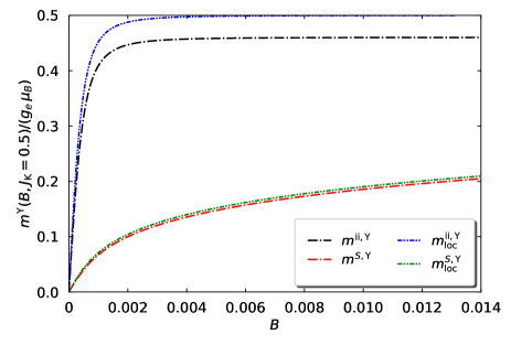
Figure 21: (Color online) Impurity spin polarization $S^{z,{\rm Y}}=m^{S,{\rm Y}}/(g_{e}\mu_{\rm B})$, eq. (14), and impurity-induced magnetization $m^{\rm ii,Y}/(g_{e}\mu_{\rm B})$, eq. (19), of the one-dimensional symmetric Kondo model as a function of global/local fields for $J_{\rm K}=0.5$ (upper figure) and $J_{\rm K}=2$ (lower figure) from the Yosida wave function.

In Fig. 21 we display the impurity spin polarization $S^{z,{\rm Y}}=m^{S,{\rm Y}}/(g_{e}\mu_{\rm B})$ and the impurity-induced magnetization $m^{\rm ii,Y}/(g_{e}\mu_{\rm B})$ from the Yosida wave function as a function of global and local magnetic fields. The curves noticeably differ from each other which shows that it is important to distinguish between the four quantities.

For small interactions, the system has a large impurity-induced magnetic susceptibility so that small fields tend to fully polarize the system. Indeed, as seen from the figure, the impurity-induced magnetization reaches its maximum value for fields of the order of $10^{-2}{\cal D}$ at $J_{\rm K}=0.5$. For these small fields, it is not important whether the field is applied globally or only locally because the magnetic response is mostly determined by the impurity spin and the electrons in its vicinity. Note that the impurity spin polarization $S^{z,{\rm Y}}$ is smaller than the impurity-induced magnetization $m^{\rm ii,Y}/(g_{e}\mu_{\rm B})$; this is an artifact of the Yosida wave function.

Large interactions, $J_{\rm K}=2$, require large fields to polarize the impurity system. Thus, the differences between the curves are more pronounced. Recall, however, that the Yosida wave function is not a good variational state for strong couplings so that the curves in Fig. 21 are not representative for the Kondo model.

A.6 Evaluation of expectation values for the Gutzwiller wave function

A.6.1 Norm, kinetic energy, and impurity spin polarization

The Gutzwiller state is normalized to unity,

$$\langle\Psi_{\rm G}|\Psi_{\rm G}\rangle=\langle\Phi|1-x(\hat{n}_{\uparrow}^{d}-n_{\uparrow}^{d,0})(\hat{n}_{\downarrow}^{d}-n_{\downarrow}^{d,0})|\Phi\rangle=1$$ (212)

because $|\Phi\rangle$ is a normalized single-particle product state and eq. (77) holds. Likewise, Linneweber et al. (2017) the expectation value of the kinetic energy in the Gutzwiller wave function gives

$$\langle\hat{T}\rangle_{\rm G} = \sum_{k,\sigma}\left(\epsilon(k)-\sigma_{n}B\right)\langle\Phi|\hat{a}_{k,\sigma}^{+}\hat{a}_{k,\sigma}^{\vphantom{+}}\hat{P}_{\rm G}^{2}|\Phi\rangle$$ (213)

$$= \sum_{k,\sigma}\left(\epsilon(k)-\sigma_{n}B\right)\langle\Phi|\hat{a}_{k,\sigma}^{+}\hat{a}_{k,\sigma}^{\vphantom{+}}|\Phi\rangle\;,$$

when we use eqs. (77) and (80). Moreover, it is readily seen from eq. (83) that

$$S^{z,{\rm G}}=\frac{1}{2}\langle\hat{n}_{\uparrow}^{d}-\hat{n}_{\downarrow}^{d}\rangle_{\rm G}=m=\frac{1}{2}\langle\Phi|\hat{n}_{\uparrow}^{d}-\hat{n}_{\downarrow}^{d}|\Phi\rangle$$ (214)

so that we do not have to distinguish between the impurity spin polarization in $|\Psi_{\rm G}\rangle$ and in $|\Phi\rangle$.

A.6.2 Spin-flip terms in the Kondo coupling

Using eq. (83) we have

$$\langle\hat{V}_{\rm sd}^{\rm sf}\rangle_{\rm G}=\lambda_{\uparrow}\lambda_{\downarrow}\frac{J_{\rm K}}{2L}\sum_{k,k^{\prime}}\langle\Phi|\left[\hat{a}_{k^{\prime},\uparrow}^{+}\hat{a}_{k,\downarrow}^{\vphantom{+}}\hat{d}_{\downarrow}^{+}\hat{d}_{\uparrow}^{\vphantom{+}}+\hbox{h.c.}\right]|\Phi\rangle\;.$$ (215)

We use Wick’s theorem for the single-particle product state $|\Phi\rangle$ to find

$$\langle\hat{V}_{\rm sd}^{\rm sf}\rangle_{\rm G} = -\frac{2}{\sqrt{1-4m^{2}}}\frac{J_{\rm K}}{2L}$$

$$\times\biggl{(}\sum_{k}\langle\Phi|\hat{d}_{\downarrow}^{+}\hat{a}_{k,\downarrow}^{\vphantom{+}}|\Phi\rangle\sum_{k^{\prime}}\langle\Phi|\hat{a}_{k^{\prime},\uparrow}^{+}\hat{d}_{\uparrow}^{\vphantom{+}}|\Phi\rangle$$

$$\hphantom{\times\biggl{(}}+\sum_{k}\langle\Phi|\hat{d}_{\uparrow}^{+}\hat{a}_{k,\uparrow}^{\vphantom{+}}|\Phi\rangle\sum_{k^{\prime}}\langle\Phi|\hat{a}_{k^{\prime},\downarrow}^{+}\hat{d}_{\downarrow}^{\vphantom{+}}|\Phi\rangle\biggr{)}\;,$$

A.6.3 Ising terms in the Kondo coupling

Using eq. (83) we have

$$\langle\hat{V}_{\rm sd}^{\rm Is}\rangle_{\rm G} = \frac{J_{\rm K}}{4L}\sum_{k,k^{\prime}}\langle\Phi|(\hat{a}_{k^{\prime},\uparrow}^{+}\hat{a}_{k,\uparrow}^{\vphantom{+}}-\hat{a}_{k^{\prime},\downarrow}^{+}\hat{a}_{k,\downarrow}^{\vphantom{+}})$$ (217)

$$\hphantom{\frac{J_{\rm K}}{4L}\sum_{k,k^{\prime}}\langle\Phi|}\biggl{(}\frac{\hat{d}_{\uparrow}^{+}\hat{d}_{\uparrow}^{\vphantom{+}}}{n_{\uparrow}^{d,0}}-\frac{\hat{d}_{\downarrow}^{+}\hat{d}_{\downarrow}^{\vphantom{+}}}{n_{\downarrow}^{d,0}}+2m\frac{\hat{n}_{\uparrow}^{d}\hat{n}_{\downarrow}^{d}}{n_{\uparrow}^{d,0}n_{\downarrow}^{d,0}}\biggr{)}|\Phi\rangle$$

$$= -\frac{J_{\rm K}}{2L}\biggl{(}\sum_{k}\langle\Phi|\hat{d}_{\uparrow}^{+}\hat{a}_{k,\uparrow}^{\vphantom{+}}|\Phi\rangle\sum_{k^{\prime}}\langle\Phi|\hat{a}_{k^{\prime},\uparrow}^{+}\hat{d}_{\uparrow}^{\vphantom{+}}|\Phi\rangle$$

$$\hphantom{-\frac{J_{\rm K}}{2L}\biggl{(}}+\sum_{k}\langle\Phi|\hat{d}_{\downarrow}^{+}\hat{a}_{k,\downarrow}^{\vphantom{+}}|\Phi\rangle\sum_{k^{\prime}}\langle\Phi|\hat{a}_{k^{\prime},\downarrow}^{+}\hat{d}_{\downarrow}^{\vphantom{+}}|\Phi\rangle\biggr{)}$$

$$+J_{\rm K}mM_{0}\;,$$

where we again used Wick’s theorem for the single-particle product state $|\Phi\rangle$, and defined the host-electron spin polarization on the impurity,

$$M_{0}=\frac{1}{2L}\sum_{k,k^{\prime}}\langle\Phi|\hat{a}_{k^{\prime},\uparrow}^{+}\hat{a}_{k,\uparrow}^{\vphantom{+}}-\hat{a}_{k^{\prime},\downarrow}^{+}\hat{a}_{k,\downarrow}^{\vphantom{+}}|\Phi\rangle\;.$$ (218)

A.7 Lagrange functional and effective non-interacting SIAM for the Gutzwiller wave function

A.7.1 Optimization of the Lagrange functional

We must optimize $\langle\hat{H}\rangle_{\rm G}$ with respect to the single-particle product states $|\Phi\rangle$ that are normalized to unity, $\langle\Phi|\Phi\rangle=1$. Moreover, we must respect the conditions (78) and (218).

We apply Ritz variational principle to the Lagrange functional ${\cal L}\equiv{\cal L}\left(\left\{|\Phi\rangle\right\},E_{\rm sp},E_{d},K\right)$, see also Ref. [Linneweber et al., 2017],

$${\cal L} = \langle\hat{H}\rangle_{\rm G}+E_{\rm sp}(1-\langle\Phi|\Phi\rangle)$$

$$+E_{d}\left(2m-\langle\Phi|\hat{n}_{\uparrow}^{d}-\hat{n}_{\downarrow}^{d}|\Phi\rangle\right)$$

$$-K\Bigl{(}2M_{0}-\frac{1}{L}\sum_{k,k^{\prime}}\langle\Phi|\hat{a}_{k^{\prime},\uparrow}^{+}\hat{a}_{k,\uparrow}^{\vphantom{+}}-\hat{a}_{k^{\prime},\downarrow}^{+}\hat{a}_{k,\downarrow}^{\vphantom{+}}|\Phi\rangle\Bigr{)}\;,$$

$$\langle\hat{H}\rangle_{\rm G} = \langle\hat{T}\rangle_{\rm G}-2mB+\langle\hat{V}_{\rm sd}^{\rm sf}\rangle_{\rm G}+\langle\hat{V}_{\rm sd}^{\rm Is}\rangle_{\rm G}\;,$$ (219)

and find that $|\Phi\rangle$ must obey the Schrödinger equation

$$\hat{H}_{0}^{\rm SIAM}|\Phi\rangle=E_{\rm sp}|\Phi\rangle$$ (220)

with the effective non-interacting single-impurity Anderson model (SIAM)

$$\hat{H}_{0}^{\rm SIAM} = \widetilde{T}+\widetilde{V}-E_{d}\left(\hat{n}_{\uparrow}^{d}-\hat{n}_{\downarrow}^{d}\right)$$ (221)

$$+\frac{K}{L}\sum_{k,k^{\prime}}\left(\hat{a}_{k^{\prime},\uparrow}^{+}\hat{a}_{k,\uparrow}^{\vphantom{+}}-\hat{a}_{k^{\prime},\downarrow}^{+}\hat{a}_{k,\downarrow}^{\vphantom{+}}\right)\;,$$

with the operators for the kinetic energy and the local hybridization

$$\widetilde{T} = \sum_{k,\sigma}(\epsilon(k)-\sigma_{n}B)\hat{a}_{k,\sigma}^{+}\hat{a}_{k,\sigma}^{\vphantom{+}}\;,$$

$$\widetilde{V} = \frac{1}{\sqrt{L}}\sum_{k,\sigma}V_{\sigma}\left(\hat{a}_{k,\sigma}^{+}\hat{d}_{\sigma}^{\vphantom{+}}+\hat{d}_{\sigma}^{+}\hat{a}_{k,\sigma}^{\vphantom{+}}\right)\;,$$ (222)

where

$$V_{\sigma} = -\frac{J_{\rm K}}{2}\left(\gamma_{\sigma}+\frac{2}{\sqrt{1-4m^{2}}}\gamma_{\bar{\sigma}}\right)\;,$$

$$\gamma_{\sigma} = \sqrt{\frac{1}{L}}\sum_{k}\langle\Phi|\hat{a}_{k,\sigma}^{+}\hat{d}_{\sigma}^{\vphantom{+}}|\Phi\rangle$$ (223)

have to be determined self-consistently. Hereby, we assumed that $\gamma_{\sigma}$ and $V_{\sigma}$ are real; recall $\bar{\uparrow}=\downarrow$, $\bar{\downarrow}=\uparrow$.

In the following we choose $|\Phi\rangle$ as the ground-state of $\hat{H}_{0}^{\rm SIAM}$ in eq. (220) and denote the optimal single-particle product state by $|\Phi_{0}\rangle$. Recall that we have to also fulfill the conditions (78) and (218),

$$m = \frac{1}{2}\langle\Phi_{0}|\hat{n}_{\uparrow}^{d}-\hat{n}_{\downarrow}^{d}|\Phi_{0}\rangle\;,$$

$$M_{0} = \frac{1}{2L}\sum_{k,k^{\prime}}\langle\Phi_{0}|\hat{a}_{k^{\prime},\uparrow}^{+}\hat{a}_{k,\uparrow}^{\vphantom{+}}-\hat{a}_{k^{\prime},\downarrow}^{+}\hat{a}_{k,\downarrow}^{\vphantom{+}}|\Phi_{0}\rangle\;,$$ (224)

which we regain from the minimization of ${\cal L}$ with respect to $E_{d}$ and $K$. The minimization of ${\cal L}$ with respect to $m$ and $M_{0}$ give

$$K = \frac{1}{2}J_{\rm K}m\;,$$

$$E_{d} = B-\frac{1}{2}J_{\rm K}M_{0}+\frac{4m}{(1-4m^{2})^{3/2}}J_{\rm K}\gamma_{\uparrow}\gamma_{\downarrow}\;.$$ (225)

Note that a finite impurity magnetization $m$ generates a potential scattering in the effective single-impurity Anderson model, $K\neq 0$.

A.7.2 Self-consistency procedure

The remaining task is the calculation of the single-particle density of states for the effective non-interacting single-impurity Anderson Hamiltonian (220). Using the single-particle density of states, we can calculate the single-particle energy $E_{\rm sp}(B,E_{d},K,V_{\sigma})$ from which we obtain $m$, $M_{0}$, and $\gamma_{\sigma}$

$$2m = -\frac{\partial E_{\rm sp}(B,E_{d},K,V_{\sigma})}{\partial E_{d}}\;,$$

$$2M_{0} = \frac{\partial E_{\rm sp}(B,E_{d},K,V_{\sigma})}{\partial K}\;,$$

$$2\gamma_{\sigma} = \frac{\partial E_{\rm sp}(B,E_{d},K,V_{\sigma})}{\partial V_{\sigma}}\;,$$ (226)

when we use the Hellmann-Feynman theorem that also holds for variational approaches. The simple proof relies on the fact that the optimized variational state is stationary with respect to small wave-function variations, see appendix B.1.

Therefore, the parameters of the single-impurity Anderson model are determined self-consistently using the following procedure.

• The self-consistency procedure is initialized by choosing the values of the paramagnetic solution, $m=0$, $M_{0}=0$, $K=0$, and $V_{\sigma}=V$, see Sect. VI.2. This guarantees that the algorithm works for $B=0$. To lift the degeneracy, we start at $E_{d}=B$ for given $B>0,J_{\rm K}>0$.

• The analytic expressions for $E_{\rm sp}(B,E_{d},K,V_{\sigma})$ give new values for $m,M_{0},\gamma_{\sigma}$ from eq. (226), and thus new values for $K$ and $E_{d}$ from eq. (225), and new values for $V_{\sigma}$ from eq. (223).

• Check whether or not $K,E_{d},V_{\sigma}$ deviate from their previous values by more than some small value $\eta=10^{-12}$. If so, return to S 2, otherwise, the algorithm terminates and gives the self-consistent values for $K,E_{d},V_{\sigma}$ and $m,M_{0},\gamma_{\sigma}$.

A.7.3 Ground-state energy

Note that $E_{\rm sp}$ is not identical to $E_{0}^{\rm G}=\langle\hat{H}_{\rm G}\rangle$. Instead, we have from eq. (222)

$$E_{\rm sp} = \langle\widetilde{T}\rangle_{0}+\langle\widetilde{V}\rangle_{0}-2mE_{d}+2KM_{0}$$ (227)

$$= \sum_{k,\sigma}(\epsilon(k)-\sigma_{n}B)\langle\Phi|\hat{a}_{k,\sigma}^{+}\hat{a}_{k,\sigma}^{\vphantom{+}}|\Phi\rangle$$

$$+\sum_{\sigma}2V_{\sigma}\gamma_{\sigma}-2mE_{d}+2KM_{0}$$

$$= \sum_{k,\sigma}(\epsilon(k)-\sigma_{n}B)\langle\Phi|\hat{a}_{k,\sigma}^{+}\hat{a}_{k,\sigma}^{\vphantom{+}}|\Phi\rangle-2mE_{d}+2KM_{0}$$

$$-J_{\rm K}\left(\gamma_{\uparrow}^{2}+\gamma_{\downarrow}^{2}+\frac{4}{\sqrt{1-4m^{2}}}\gamma_{\uparrow}\gamma_{\downarrow}\right)\;,$$

where we used eq. (223) to replace $V_{\sigma}$ by $\gamma_{\sigma}$. In contrast, from eq. (219) we have

$$E_{0}^{\rm G} = \sum_{k,\sigma}(\epsilon(k)-\sigma_{n}B)\langle\Phi|\hat{a}_{k,\sigma}^{+}\hat{a}_{k,\sigma}^{\vphantom{+}}|\Phi\rangle-m(2B-J_{\rm K}M_{0})$$ (228)

$$-\frac{J_{\rm K}}{2}\left(\frac{4}{\sqrt{1-4m^{2}}}\gamma_{\downarrow}\gamma_{\uparrow}+\gamma_{\uparrow}^{2}+\gamma_{\downarrow}^{2}\right)\;.$$

Comparing both equations results in

$$E_{0}^{\rm G} = E_{\rm sp}+\frac{J_{\rm K}}{2}\left(\frac{4}{\sqrt{1-4m^{2}}}\gamma_{\downarrow}\gamma_{\uparrow}+\gamma_{\uparrow}^{2}+\gamma_{\downarrow}^{2}\right)$$ (229)

$$-m(2B-J_{\rm K}M_{0})+2mE_{d}-2KM_{0}$$

$$= E_{\rm sp}+\frac{J_{\rm K}}{2}\left(\frac{4}{\sqrt{1-4m^{2}}}\gamma_{\downarrow}\gamma_{\uparrow}+\gamma_{\uparrow}^{2}+\gamma_{\downarrow}^{2}\right)$$

$$+\frac{8m^{2}}{(1-4m^{2})^{3/2}}J_{\rm K}\gamma_{\uparrow}\gamma_{\downarrow}-J_{\rm K}mM_{0}$$

for the Gutzwiller variational ground-state energy of the Kondo model. The excess ground-state energy for the Gutzwiller variational state is given by

$$e_{0}^{\rm G}(J_{\rm K},B) = E_{0}^{\rm G}(J_{\rm K},B)$$

$$-\sum_{k,\sigma}(\epsilon(k)-\sigma_{n}B)\langle\hbox{FS}|\hat{a}_{k,\sigma}^{+}\hat{a}_{k,\sigma}^{\vphantom{+}}|\hbox{FS}\rangle\;,$$

where $|\hbox{FS}\rangle$ is the Fermi sea of non-interacting electrons.

The variational optimization for $m>0$ is outlined in appendix B.4. Here, we summarize the main results.

• The Gutzwiller ground state displays a finite local magnetization, $m>0$, at $B=0^{+}$ for all $0<J_{\rm K}<J_{\rm K,c}^{\rm G}\approx 0.839$. The precise value is determined in Sect. A.8.7.

• For small interactions, $J_{\rm K}\to 0$, the values for $V_{\sigma}$, $\gamma_{\sigma}$ $E_{d}$, $K$, $m$, $M_{0}$, and $\omega_{p,\downarrow}$ can be determined analytically.

• The ground-state energy for small interactions in one dimension can be approximated by

  $$e_{0}^{\rm G}(J_{\rm K})\approx-0.0905J_{\rm K}^{2}-0.051J_{\rm K}^{3}-0.05J_{\rm K}^{4}$$ (231)

  for the Gutzwiller variational energy for $J_{\rm K}\lesssim 0.4$. The quadratic coefficient can be compared with the exact result from perturbation theory, $e_{0}(J_{\rm K})\approx-3J_{\rm K}^{2}/32=-0.09375J_{\rm K}^{2}$, see eq. (34). The magnetic Gutzwiller states accounts for 96.5% of the correlation energy.

A.8 Zero-field impurity spin susceptibility for the paramagnetic Gutzwiller state

From the numerical solution of the self-consistency equations, we see that $\gamma_{\uparrow}=\gamma_{\downarrow}$ and $V_{\uparrow}=V_{\downarrow}$ at self-consistency. In the following, we use this assumption.

A.8.1 Impurity spin polarization

The optimization procedure of Sect. A.7 directly gives the impurity spin polarization,

$$\frac{m^{S,{\rm G}}(J_{\rm K},B)}{g_{e}\mu_{\rm B}}=m(J_{\rm K},B)\;.$$ (232)

When the external field is applied only at the impurity, we simply replace the expression $(\epsilon(k)-\sigma_{n}B)$ by $\epsilon(k)$ in eqs. (213), (222), (227), (228), and (A.7.3) to arrive at the corresponding ‘local’ expressions for the impurity spin polarization and impurity-induced magnetization. Invoking the variational Hellmann-Feynman theorem, Hellmann (2015); Feynman (1939) see appendix B.1, we may alternatively use

$$\frac{m^{{\rm S,G}}_{\rm loc}(J_{\rm K},B)}{g_{e}\mu_{\rm B}}=-\frac{1}{2}\frac{\partial e_{0,{\rm loc}}^{\rm G}(J_{\rm K},B)}{\partial B}\;,$$ (233)

see also eq. (22).

A.8.2 Impurity-induced magnetization

Following the steps in Sect. A.6 it is readily shown that

$$\frac{m^{\rm ii,G}(J_{\rm K},B)}{g_{e}\mu_{\rm B}}=\langle\Phi_{0}|\hat{S}^{z}+\hat{s}^{z}|\Phi_{0}\rangle-\langle\text{FS}|\hat{s}^{z}|\text{FS}\rangle\;.$$ (234)

Here, $|\Phi_{0}\rangle$ is the optimized ground state of the effective non-interacting single-impurity Anderson model Hamiltonian defined in eq. (221) and $|\text{FS}\rangle$ is the Fermi-sea ground state of non-interacting electrons in the presence of a magnetic field. When we use the single-particle density of states of the non-interacting SIAM, see appendix B.4, we find

$$\frac{m^{\rm ii,G}(J_{\rm K},B)}{g_{e}\mu_{\rm B}} = \frac{1}{2}\int_{-\infty}^{0}{\rm d}\omega\left(D_{\uparrow}(\omega)-D_{\downarrow}(\omega)\right)$$

$$-\frac{1}{2}\int_{-\infty}^{0}{\rm d}\omega\left(D^{\rm FS}_{\uparrow}(\omega)-D^{\rm FS}_{\downarrow}(\omega)\right)$$

$$= \frac{1}{2}\int_{-\infty}{\rm d}\omega\left(D_{{\rm imp},\uparrow}(\omega)-D_{{\rm imp},\downarrow}(\omega)\right)\;,$$

where the impurity density of states is given by the phase-shift function

$$D_{{\rm imp},\sigma}(\omega) = -\frac{1}{\pi}\frac{\partial\varphi_{\sigma}(\omega,B,E_{d},K,V)}{\partial\omega}\;,$$

$$\cot[\varphi_{\sigma}(\omega,B,E_{d},K,V)] = \frac{{\rm R}_{\sigma}(\omega)}{{\rm I}_{\sigma}(\omega)}\;,$$ (236)

with the real and imaginary parts of the hybridization function

$${\rm R}_{\sigma}(\omega) = (\omega+\sigma_{n}E_{d})(1-\sigma_{n}K\Lambda_{0}(\omega+\sigma_{n}B))$$

$$-V^{2}\Lambda_{0}(\omega+\sigma_{n}B)\;,$$

$${\rm I}_{\sigma}(\omega) = \eta\left(1-\sigma_{n}K\Lambda_{0}(\omega+\sigma_{n}B)\right)$$

$$+\left[(\omega+\sigma_{n}E_{d})\sigma_{n}K+V^{2}\right]\pi\rho_{0}(\omega+\sigma_{n}B)\;,$$

see eqs. (IV-43) and (IV-44) of the supplemental material, and $\eta=0^{+}$.

Since the impurity contribution to the density of states is given by a frequency derivative, the frequency integration in eq. (LABEL:eq:miiGfromDOS) is readily carried out. The density of states vanishes for $\omega\to-\infty$ so that the density of states at the Fermi energy alone determines the impurity-induced magnetization. We focus on the paramagnetic region for the Gutzwiller wave function, $J_{\rm K}>J_{\rm K,c}^{\rm G}$, so that the band part of the impurity density of states at the Fermi energy gives, see eq. (IV-50) of the supplemental material,

$$\frac{m^{\rm ii,G}(J_{\rm K},B)}{g_{e}\mu_{\rm B}} = -\frac{1}{2\pi}\left(X_{\uparrow}(0)-X_{\downarrow}(0)\right)\;,$$

$$X_{\sigma}(\omega) \equiv X_{\sigma}(\omega,B,E_{d},K,V)$$

$$= \pi\theta_{\rm H}(-\omega-\sigma_{n}E_{d})$$

$$+{\rm arccot}\biggl{[}\frac{(\omega+\sigma_{n}E_{d})\sqrt{1-(\omega+\sigma_{n}B)^{2}}}{(\omega+\sigma_{n}E_{d})\sigma_{n}K+V^{2}}\biggr{]}$$

in one dimension. Thus, we obtain the final result

$$\frac{m^{\rm ii,G}(J_{\rm K},B)}{g_{e}\mu_{\rm B}} = \frac{1}{2}-\frac{1}{\pi}{\rm arccot}\left[\frac{E_{d}\sqrt{1-B^{2}}}{E_{d}K+V^{2}}\right]$$ (239)

$$= \frac{1}{\pi}\arctan\left[\frac{E_{d}\sqrt{1-B^{2}}}{E_{d}K+V^{2}}\right]\;,$$

where $E_{d}(B)$, $K(B)$, and $V(B)$ are determined from the solution of the self-consistency cycle in Sect. A.7.

When the field is only applied locally, the same considerations lead to

$$\frac{m^{\rm ii,G}_{\rm loc}(J_{\rm K},B)}{g_{e}\mu_{\rm B}}=\frac{1}{\pi}\arctan\left[\frac{E_{d,{\rm loc}}}{E_{d,{\rm loc}}K_{\rm loc}+V_{\rm loc}^{2}}\right]\;,$$ (240)

where the self-consistency problem has to be solved for a local field only. We show the impurity spin polarization and the impurity-induced magnetization as a function of an applied global/local magnetic field in Fig. 22 for $J_{\rm K}=1$, where the Gutzwiller wave function describes a local spin singlet.

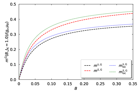
Figure 22: (Color online) Impurity spin polarization $S^{z,{\rm G}}=m^{S,{\rm G}}/(g_{e}\mu_{\rm B})$, eqs. (232) and (233), and impurity-induced magnetization $m^{\rm ii,G}/(g_{e}\mu_{\rm B})$, eqs. (239) and (240), of the one-dimensional symmetric Kondo model as a function of global/local fields for $J_{\rm K}=1$ from the Gutzwiller wave function.

In contrast to the Yosida wave function, the Gutzwiller wave function correctly shows that the impurity spin polarization is larger than the impurity-induced magnetization because the impurity spin is surrounded by a cloud of conduction electrons that screens the impurity spin. As in the Yosida wave function, the impurity spin polarization does not depend much on whether the magnetic field is applied globally of locally.

A.8.3 Small fields

In the paramagnetic phase, $J_{\rm K}>J_{\rm K,c}^{\rm G}$, and for small fields, $B\to 0$, we can derive explicit results for the zero-field impurity spin susceptibility because it is sufficient to solve the self-consistency equations to linear order in the external field.

Keeping all terms up to linear order in $B$, we make the Ansatz

$$\omega_{p,\uparrow} = \omega_{p}+\bar{\omega}_{p}B\;,$$

$$\omega_{p,\downarrow} = \omega_{p}-\bar{\omega}_{p}B\;,$$

$$K = \bar{K}B\;,$$

$$E_{d} = \bar{E}_{d}B\;,$$

$$M_{0} = \bar{M}_{0}B\;,$$

$$m = 2\chi B\;,$$ (241)

where $\chi$ is the desired zero-field impurity-spin susceptibility in units of $(g_{e}\mu_{\rm B})^{2}$,

$$\frac{\chi_{0}^{S,{\rm G}}(J_{\rm K},B)}{(g_{e}\mu_{\rm B})^{2}}=\chi\;.$$ (242)

In one dimension at $B=0$, the pole is at $\omega_{p}=-v_{+}$, see eq. (85). Moreover, from eq. (21) and eq. (239) we find

$$\frac{\chi_{0}^{\rm ii,G}(J_{\rm K})}{(g_{e}\mu_{\rm B})^{2}}=\frac{\bar{E}_{d}}{2\pi V^{2}}\;,$$ (243)

where $V_{\uparrow}=V_{\downarrow}=V$ and $\gamma_{\uparrow}=\gamma_{\downarrow}=\gamma=-2V/(3J_{\rm K})$, with corrections of the order $B^{2}$, and with

$$J_{\rm K}(V)=-\frac{8V}{3}\left(\frac{\partial e_{0}(V)}{\partial V}\right)^{-1}\;,$$ (244)

where $V$ instead of $J_{\rm K}$ parameterizes the strength of the Kondo interaction. For $e_{0}(V)$, see eq. (84).

Apparently, we have five unknowns, namely

$$\underline{v}^{\rm T}=\left(\bar{\omega}_{p},\bar{E}_{d},\bar{K},\bar{M}_{0},\chi\right)\;,$$ (245)

and we need five independent linear equations that connect these quantities.

A.8.4 Useful integrals

For later use we define the following set of integrals,

$$J_{n}(V)=\int_{-1}^{0}\frac{{\rm d}\omega}{\pi}\frac{\omega^{n}\sqrt{1-\omega^{2}}}{(\omega^{2}-\omega^{4}+V^{4})^{2}}\;.$$ (246)

Using Mathematica Wolfram Research, Inc. (2016) the required integrals read

$$J_{1}(V) = -\frac{1}{2\pi V^{4}(1+4V^{4})}$$ (247)

$$+\frac{\left(-2+\sqrt{1+4V^{4}}\right)\arctan(1/v_{-})}{2\pi v_{-}(1+4V^{4})^{3/2}}$$

$$+\frac{\left(2+\sqrt{1+4V^{4}}\right)}{4\pi v_{+}(1+4V^{4})^{3/2}}\ln\left(\frac{v_{+}-1}{v_{+}+1}\right)$$

and

$$J_{3}(V) = \frac{1}{\pi(1+4V^{4})}$$

$$+\frac{(-3-4V^{4}+\sqrt{1+4V^{4}})\arctan(1/v_{-})}{4\pi v_{-}(1+4V^{4})^{3/2}}$$

$$+\frac{\left(3+4V^{4}+\sqrt{1+4V^{4}}\right)}{8\pi v_{+}(1+4V^{4})^{3/2}}\ln\left(\frac{v_{+}-1}{v_{+}+1}\right)\;.$$

For $v_{\pm}$, see eq. (85).

A.8.5 Five equations

As shown in appendix B.4,

$$\bar{E}_{d}=1-\frac{J_{\rm K}}{2}\bar{M}_{0}+8J_{\rm K}\chi\gamma^{2}$$ (249)

with $\gamma=-2V/(3J_{\rm K})$,

$$\bar{K}=J_{\rm K}\chi\;,$$ (250)

$$\bar{E}_{d}(\omega_{p}^{2}-1)+(2\omega_{p}^{2}-1)\bar{\omega}_{p}+\omega_{p}^{2}-\bar{K}V^{2}=0\;,$$ (251)

$$\bar{M}_{0} = \bar{M}_{0}^{\rm b}+\bar{M}_{0}^{\rm band}\;,$$ (252)

$$\bar{M}_{0}^{\rm b} = \frac{\bar{K}(-\omega_{p}^{2}+2\omega_{p}^{4}+V^{4})-\omega_{p}^{2}(3+\bar{E}_{d}+4\bar{\omega}_{p})V^{2}}{\omega_{p}(1-2\omega_{p}^{2})^{2}}$$

$$\bar{M}_{0}^{\rm band} = -2\bar{K}V^{2}J_{3}(V)+2\left(\bar{E}_{d}-1\right)V^{4}J_{1}(V)\;,$$

$$\chi = \chi^{\rm b}+\chi^{\rm band}\;,$$ (253)

$$\chi^{\rm b} = \frac{\omega_{p}(1+\bar{E}_{d}+\omega_{p}^{2}-\bar{E}_{d}\omega_{p}^{2}+2\bar{\omega}_{p}-\bar{K}V^{2})}{2(1-2\omega_{p}^{2})^{2}}\;,$$

$$\chi^{\rm band} = \frac{1}{2\pi V^{2}}$$

$$-V^{2}\left[\left(\bar{E}_{d}-1\right)(J_{1}(V)-J_{3}(V))+\bar{K}V^{2}J_{1}(V)\right]\,.$$

Eqs. (249)–(253) are the required five equations for the five unknowns in eq. (245).

A.8.6 Matrix problem

The resulting matrix problem reads with $\omega_{p}=-v_{+}$, see eq. (85), and with $\underline{v}$ from eq. (245)

$$\underline{\underline{M}}\cdot\underline{v}=\underline{g}\;.$$ (254)

Here, the matrix has the form

$$\underline{\underline{M}}=\left(\begin{array}[]{@{}ccccc@{}}0&1&0&J_{\rm K}/2&-8J_{\rm K}\gamma^{2}\\ 0&0&1&0&-J_{\rm K}\\ 2\omega_{p}^{2}-1&\omega_{p}^{2}-1&-V^{2}&0&0\\ M_{41}&M_{42}&M_{43}&-1&0\\ M_{51}&M_{52}&M_{53}&0&-1\end{array}\right)$$ (255)

with the matrix elements

$$M_{41} = -\frac{4\omega_{p}V^{2}}{(1-2\omega_{p}^{2})^{2}}\;,$$

$$M_{42} = -\frac{\omega_{p}V^{2}}{(1-2\omega_{p}^{2})^{2}}+2V^{4}J_{1}(V)\;,$$

$$M_{43} = \frac{(-\omega_{p}^{2}+2\omega_{p}^{4}+V^{4})}{\omega_{p}(1-2\omega_{p}^{2})^{2}}-2V^{2}J_{3}(V)\;,$$

$$M_{51} = \frac{\omega_{p}}{(1-2\omega_{p}^{2})^{2}}\;,$$

$$M_{52} = \frac{\omega_{p}(1-\omega_{p}^{2})}{2(1-2\omega_{p}^{2})^{2}}-V^{2}\left(J_{1}(V)-J_{3}(V)\right)\;,$$

$$M_{53} = -\frac{V^{2}\omega_{p}}{2(1-2\omega_{p}^{2})^{2}}-V^{4}J_{1}(V)\;.$$ (256)

For a global external field, the inhomogeneity reads

$$\underline{g}^{\rm T}=\left(1,0,-\omega_{p}^{2},g_{4},g_{5}\right)\;,$$ (257)

where

$$g_{4} = \frac{3\omega_{p}V^{2}}{(1-2\omega_{p}^{2})^{2}}+2V^{4}J_{1}(V)\;,$$

$$g_{5} = -\frac{\omega_{p}(1+\omega_{p}^{2})}{2(1-2\omega_{p}^{2})^{2}}$$ (258)

$$-V^{2}\left(J_{1}(V)-J_{3}(V)\right)-\frac{1}{2\pi V^{2}}\;.$$

When the external field is applied only locally, the matrix $\underline{\underline{M}}$ and the vector $\underline{v}$ in eq. (254) remain unchanged but we have for the inhomogeneity

$$\underline{g}_{\rm loc}^{\rm T}=\left(1,0,0,0,0\right)\;.$$ (259)

The matrix problem (254) can be solved analytically, generating large expressions. Eventually, we solve it numerically.

A.8.7 Strong-coupling limit

For the non-trivial entries in the matrix $\underline{\underline{M}}$ we have

$$M_{14} = \frac{2V}{3}+\frac{1}{6V}-\frac{4}{9\pi V^{2}}+\frac{5}{48V^{3}}\;,$$

$$M_{15} = -\frac{8V}{3}+\frac{2}{3V}-\frac{16}{9\pi V^{2}}+\frac{1}{4V^{3}}\;,$$

$$M_{25} = -\frac{4V}{3}-\frac{1}{3V}+\frac{8}{9\pi V^{2}}-\frac{5}{24V^{3}}\;,$$

$$M_{31} = 2V^{2}+\frac{1}{4V^{2}}\;,$$

$$M_{32} = V^{2}-\frac{1}{2}+\frac{1}{8V^{2}}\;,$$

$$M_{33} = -V^{2}\;,$$

$$M_{41} = \frac{1}{V}+\frac{1}{4V^{3}}\;,$$

$$M_{42} = \frac{1}{4V}+\frac{1}{16V^{3}}\;,$$ (260)

and

$$M_{43} = -\frac{3}{4V}-\frac{1}{16V^{3}}\;,$$

$$M_{51} = -\frac{1}{4V^{3}}\;,$$

$$M_{52} = \frac{1}{8V}-\frac{1}{32V^{3}}\;,$$

$$M_{53} = \frac{1}{8V}+\frac{1}{32V^{3}}\;,$$ (261)

up to and including order $1/V^{3}$. To the same order,

$$\underline{g}^{\rm T} = \Bigl{(}1,0,-V^{2}-1/2-1/(8V^{2}),-3/(4V)-3/(16V^{3}),$$ (262)

$$\hphantom{\Bigl{(}}1/(8V)-1/(2\pi V^{2})+7/(32V^{3})\Bigr{)}^{\rm T}\;.$$

Lastly, for $J_{\rm K}\gg 1$ we have from eq. (LABEL:eq:VlargeGutz)

$$V(J_{\rm K})=\frac{3}{4}J_{\rm K}-\frac{1}{3J_{\rm K}}+\frac{32}{27\pi J_{\rm K}^{2}}-\frac{14}{27J_{\rm K}^{3}}+{\cal O}(1/J_{\rm K}^{4})\;.$$ (263)

Then, Mathematica Wolfram Research, Inc. (2016) gives the vector $\underline{v}$,

$$\underline{v}^{\rm T} = \left(\bar{\omega}_{p},\bar{E}_{d},\bar{K},\bar{M}_{0},\chi\right)$$ (264)

$$= \Bigl{(}-1-\frac{4}{3\pi V}+\frac{29}{18\pi V^{3}},1+\frac{13}{3\pi V}-\frac{7}{36\pi V^{3}},$$

$$\hphantom{\Bigl{(}}\frac{5}{3\pi V}+\frac{31}{36\pi V^{3}},-\frac{3}{2\pi V^{2}},\frac{5}{4\pi V^{2}}\Bigr{)}^{\rm T}\;,$$

up to and including order $1/V^{3}$. Thus, the strong-coupling limit of the impurity spin susceptibility in the Gutzwiller wave function is given by

$$\frac{\chi_{0}^{S,{\rm G}}(J_{\rm K}\gg 1)}{(g_{e}\mu_{\rm B})^{2}}=\frac{5}{4\pi V^{2}}+{\cal O}(1/V^{4})=\frac{20}{9\pi J_{\rm K}^{2}}+{\cal O}(1/J_{\rm K}^{4})\;.$$ (265)

For a local external field we obtain in the strong-coupling limit

$$\underline{v}_{\rm loc}^{\rm T} = \Bigl{(}-1+\frac{7}{12V^{2}}-\frac{1}{3\pi V^{3}},\frac{5}{2}+\frac{2}{3V^{2}}+\frac{1}{3\pi V^{3}},$$ (266)

$$\hphantom{\Bigl{(}}\frac{1}{2}+\frac{7}{12V^{2}}-\frac{1}{3\pi V^{3}},-\frac{3}{4V}+\frac{3}{16V^{3}},$$

$$\hphantom{\Bigl{(}}\frac{3}{8V}+\frac{11}{32V^{3}}\Bigr{)}^{\rm T}\;,$$

up to and including order $1/V^{3}$. Thus, for a local magnetic field, the strong-coupling limit of the impurity spin susceptibility in the Gutzwiller wave function is given by

$$\frac{\chi_{0,{\rm loc}}^{S,{\rm G}}(J_{\rm K}\gg 1)}{(g_{e}\mu_{\rm B})^{2}}=\frac{3}{8V}+\frac{11}{32V^{3}}=\frac{1}{2J_{\rm K}}+\frac{28}{27J_{\rm K}^{3}}+{\cal O}(1/J_{\rm K}^{4})\;.$$ (267)

For the zero-field impurity-induced susceptibilities in eq. (243) we find in the strong-coupling limit

$$\frac{\chi_{0}^{\rm ii,G}(J_{\rm K}\gg 1)}{(g_{e}\mu_{\rm B})^{2}} = \frac{1}{2\pi V^{2}}\biggl{[}1+\frac{13}{3\pi V}-\frac{7}{36\pi V^{3}}+{\cal O}(V^{-4})\biggr{]}$$ (268)

$$= \frac{8}{9\pi J_{\rm K}^{2}}+\frac{416}{81\pi^{2}J_{\rm K}^{3}}+{\cal O}(1/J_{\rm K}^{4})$$

and

$$\frac{\chi_{0,{\rm loc}}^{\rm ii,G}(J_{\rm K}\gg 1)}{(g_{e}\mu_{\rm B})^{2}} = \frac{1}{2\pi V^{2}}\biggl{[}\frac{5}{2}+\frac{2}{3V^{2}}+\frac{1}{3\pi V^{3}}+{\cal O}(V^{-4})\biggr{]}$$ (269)

$$= \frac{20}{9\pi J_{\rm K}^{2}}+{\cal O}(1/J_{\rm K}^{4})\;.$$

The impurity spin susceptibility for a local field goes to zero proportional to $1/J_{\rm K}$, all other susceptibilities vanish proportional to $J_{\rm K}^{-2}$. From eqs. (265) and (269) we see that $\chi_{0}^{S,{\rm G}}(J_{\rm K})$ and $\chi_{0,{\rm loc}}^{\rm ii,G}(J_{\rm K})$ agree to order $J_{\rm K}^{-2}$. A closed inspection shows that the expressions indeed agree to order $J_{\rm K}^{-4}$.

A.9 Hamiltonian of the Wilson chain

The matrix elements are calculated recursively from the starting values

$$\varepsilon_{0,\sigma} = \int_{-1-\sigma_{n}B}^{1-\sigma_{n}B}{\rm d}\epsilon\,\epsilon\,\rho_{0}(\epsilon+\sigma_{n}B)\;,$$

$$t_{0,\sigma}^{2} = \sum_{m}\Bigl{[}(\zeta_{m,\sigma}^{+}-\varepsilon_{0,\sigma})^{2}(\gamma^{+}_{m,\sigma})^{2}$$

$$\hphantom{\sum_{m}\Bigl{[}}+(\zeta_{m,\sigma}^{-}-\varepsilon_{0,\sigma})^{2}(\gamma^{-}_{m,\sigma})^{2}\Bigr{]}\;,$$

$$u_{0,m,\sigma} = \gamma_{m,\sigma}^{+}\;,$$

$$v_{0,m,\sigma} = \gamma_{m,\sigma}^{-}\;,$$

$$u_{1,m,\sigma} = \frac{(\zeta^{+}_{m,\sigma}-\varepsilon_{0,\sigma})u_{0,m,\sigma}}{t_{0,\sigma}}\;,$$

$$v_{1,m,\sigma} = \frac{(\zeta^{-}_{m,\sigma}-\varepsilon_{0,\sigma})v_{0,m,\sigma}}{t_{0,\sigma}}\;.$$ (270)

For $n\geq 1$ one has to calculate iteratively

$$\varepsilon_{n,\sigma} = \sum_{m}\zeta_{m,\sigma}^{+}u_{n,m,\sigma}^{2}+\zeta_{m,\sigma}^{-}u_{n,m,\sigma}^{2}\;,$$

$$t_{n,\sigma}^{2} = \sum_{m}\left[(\zeta^{+}_{m,\sigma})^{2}u^{2}_{n,m,\sigma}+(\zeta^{-}_{m,\sigma})^{2}v^{2}_{n,m,\sigma}\right]$$ (271)

$$-t_{n-1,\sigma}^{2}-\varepsilon_{n,\sigma}^{2}\;,$$

and

$$u_{n+1,m,\sigma} = \frac{(\zeta_{m,\sigma}^{+}-\varepsilon_{n,\sigma})u_{n,m,\sigma}-t_{n-1,\sigma}u_{n-1,m,\sigma}}{t_{n,\sigma}}\;,$$

$$v_{n+1,m,\sigma} = \frac{(\zeta_{m,\sigma}^{-}-\varepsilon_{n,\sigma})v_{n,m,\sigma}-t_{n-1,\sigma}v_{n-1,m,\sigma}}{t_{n,\sigma}}\;.$$

This concludes the derivation of the Wilson chain Hamiltonian.

Appendix B Outline of the supplemental material

In this appendix, we summarize the content of the supplemental material.

B.1 Hellmann-Feynman theorem

We formulate and prove the Hellmann-Feynman theorem and its variational counterpart.

B.2 Lanczos approach

We recapitulate the Lanczos approach and show its variational property. Moreover, we calculate the first-order Lanczos coefficients for a constant and a one-dimensional density of states.

B.3 Scattering off a local impurity

We calculate the single-particle Green function for electrons that scatter off a local potential. The results permit the calculation of the ground-state energy of the Kondo model for large Kondo couplings.

B.4 Non-interacting SIAM in the presence of potential scattering and a magnetic field

We calculate the single-particle Green function for electrons in the non-interacting single-impurity Anderson model in the presence of a magnetic field and a local scattering potential. We use it to calculate the ground-state energy, the magnetization, and the zero-field susceptibility in the SIKM for the Gutzwiller wave function.

B.5 Ground-state energy from Bethe Ansatz

We collect the Bethe Ansatz equations and use them to derive the ground-state energy. Unfortunately, the Bethe Ansatz does not provide tangible results for this quantity because the Bethe Ansatz energy is of third order in the Kondo coupling.

B.6 Free energy in second-order weak-coupling perturbation theory

We re-derive the expressions for the free energy to second order in the Kondo coupling at finite temperature and external magnetic field for a general density of states of the host electrons. These results are used to calculate the Wilson number and the dominant term in the zero-field susceptibilities whereby we generalize previous results in the literature.

Supplemental material
Symmetric single-impurity Kondo model on a tight-binding chain:
a comparison of analytical and numerical ground-state approaches
Gergely Barcza, Kevin Bauerbach, Fabian Eickhoff, Frithjof B. Anders, Florian Gebhard, Örs Legeza

The supplemental material consists of six parts. In supplement I, we formulate and prove the Hellmann-Feynman theorem and its variational counterpart. In supplement II, we recapitulate the Lanczos approach and show its variational property. Moreover, we calculate the first-order Lanczos coefficients for a constant and a one-dimensional density of states. In supplement III, we calculate the single-particle Green function for electrons that scatter off a local potential. The results permit the calculation of the ground-state energy of the Kondo model for large Kondo couplings. In supplement IV, we calculate the single-particle Green function for electrons in the non-interacting single-impurity Anderson model in the presence of a magnetic field and a local scattering potential. We use it to calculate the magnetization and the zero-field susceptibility in the SIKM for the Gutzwiller wave function. We also discuss the magnetic transition in the Gutzwiller wave function. In supplement V, we collect the Bethe Ansatz equations and use them to derive the ground-state energy. Unfortunately, the Bethe Ansatz does not provide tangible results for this quantity. In supplement VI, we re-derive the expressions for the free energy to second order in the Kondo coupling at finite temperature and external magnetic field for a general density of states of the host electrons. These results are used to calculate the Wilson number and the dominant term in the zero-field susceptibilities whereby we generalize previous results in the literature.

Supplement I Hellmann-Feynman theorem

In preparation for the variational Hellmann-Feynman theorem, we first recapitulate the proof of the theorem for the exact ground state, and then move on to its variational counterpart.

I.1 Exact ground state

Let $|\Psi_{0}(\lambda)\rangle$ be the exact ground state of the Hamiltonian $\hat{H}(\lambda)$,

$$\hat{H}(\lambda)|\Psi_{0}(\lambda)\rangle=E_{0}(\lambda)|\Psi_{0}(\lambda)\rangle\;,$$ (I-273)

where $\lambda$ is some real parameter, e.g., the interaction strength. Taking the derivative with respect to $\lambda$ results in

$$\frac{\partial\hat{H}(\lambda)}{\partial\lambda}|\Psi_{0}(\lambda)\rangle = \left(E_{0}(\lambda)-\hat{H}(\lambda)\right)|\dot{\Psi}_{0}(\lambda)\rangle$$ (I-274)

$$+\frac{\partial E_{0}(\lambda)}{\partial\lambda}|\Psi_{0}(\lambda)\rangle\;,$$

where the dot on the wave function implies the derivative with respect to $\lambda$. We multiply this equation with $\langle\Psi_{0}(\lambda)|$ and use the Schrödinger equation (I-273) to find

$$\langle\Psi_{0}(\lambda)|\frac{\partial\hat{H}(\lambda)}{\partial\lambda}|\Psi_{0}(\lambda)\rangle=\langle\Psi_{0}(\lambda)|\frac{\partial E_{0}(\lambda)}{\partial\lambda}|\Psi_{0}(\lambda)\rangle$$ (I-275)

or

$$\frac{\partial E_{0}(\lambda)}{\partial\lambda}=\frac{\langle\Psi_{0}(\lambda)|\frac{\displaystyle\partial\hat{H}(\lambda)}{\displaystyle\partial\lambda}|\Psi_{0}(\lambda)\rangle}{\langle\Psi_{0}(\lambda)|\Psi_{0}(\lambda)\rangle}\;,$$ (I-276)

which constitutes the Hellmann-Feynman theorem. Hellmann (2015); Feynman (1939)

I.2 Variational state

The variationally optimized state $|\Phi_{\rm G}(\lambda)\rangle$ provides an upper bound to the ground-state energy of $\hat{H}(\lambda)$,

$$E_{0}(\lambda)\leq E_{0}^{\rm var}(\lambda)=\frac{\langle\Phi_{\rm G}(\lambda)|\hat{H}(\lambda)|\Phi_{\rm G}(\lambda)\rangle}{\langle\Phi_{\rm G}(\lambda)|\Phi_{\rm G}(\lambda)\rangle}\;.$$ (I-277)

The variational optimization implies that a linear deviation from $|\Phi_{\rm G}(\lambda)\rangle$ results in a quadratic change in the variational energy,

$$\frac{\langle\Phi_{\rm G}(\lambda)+\delta\Phi|\hat{H}(\lambda)|\Phi_{\rm G}(\lambda)+\delta\Phi\rangle}{\langle\Phi_{\rm G}(\lambda)+\delta\Phi|\Phi_{\rm G}(\lambda)+\delta\Phi\rangle}=E_{0}^{\rm var}(\lambda)+{\cal O}\left((\delta\Phi)^{2}\right)\,.$$ (I-278)

We shift $\lambda$ by $({\rm d}\lambda)$ in eq. (I-277) to find up to linear order in $({\rm d}\lambda)$

lhs $$= \hbox{rhs}\;,$$

lhs $$= E_{0}^{\rm var}(\lambda)+\frac{\partial E_{0}^{\rm var}(\lambda)}{\partial\lambda}({\rm d}\lambda)\;,$$

rhs $$= \frac{\langle\Phi_{\rm G}(\lambda+{\rm d}\lambda)|\hat{H}(\lambda)|\Phi_{\rm G}(\lambda+{\rm d}\lambda)\rangle}{\langle\Phi_{\rm G}(\lambda+{\rm d}\lambda)|\Phi_{\rm G}(\lambda+{\rm d}\lambda)\rangle}$$ (I-279)

$$+\frac{\langle\Phi_{\rm G}(\lambda)|\frac{\displaystyle\partial\hat{H}(\lambda)}{\displaystyle\partial\lambda}|\Phi_{\rm G}(\lambda)\rangle}{\langle\Phi_{\rm G}(\lambda)|\Phi_{\rm G}(\lambda)\rangle}({\rm d}\lambda)$$

$$= E_{0}^{\rm var}(\lambda)+{\cal O}\left(({\rm d}\lambda)^{2}\right)$$

$$+\frac{\langle\Phi_{\rm G}(\lambda)|\frac{\displaystyle\partial\hat{H}(\lambda)}{\displaystyle\partial\lambda}|\Phi_{\rm G}(\lambda)\rangle}{\langle\Phi_{\rm G}(\lambda)|\Phi_{\rm G}(\lambda)\rangle}({\rm d}\lambda)\;,$$

where we used eq. (I-278) in the last step; note that $|\delta\Phi\rangle=|\Phi_{\rm G}(\lambda+{\rm d}\lambda)\rangle-|\Phi_{\rm G}(\lambda)\rangle$ is proportional to $({\rm d}\lambda)$. Therefore, we obtain the variational Hellmann-Feynman theorem,

$$\frac{\partial E_{0}^{\rm var}(\lambda)}{\partial\lambda}=\frac{\langle\Phi_{\rm G}(\lambda)|\frac{\displaystyle\partial\hat{H}(\lambda)}{\displaystyle\partial\lambda}|\Phi_{\rm G}(\lambda)\rangle}{\langle\Phi_{\rm G}(\lambda)|\Phi_{\rm G}(\lambda)\rangle}\;.$$ (I-280)

Supplement II Lanczos approach

II.1 Lanczos method

Let $\hat{H}$ be the Hamiltonian of the system and let $|\Psi_{0}\rangle$ be its (non-degenerate) ground state,

$$\hat{H}|\Psi_{0}\rangle=E_{0}|\Psi_{0}\rangle\;,$$ (II-281)

where $E_{0}$ is the exact ground-state energy. Moreover, we assume that the Hilbert space of dimension $d=\hbox{dim}(\hat{H})$ does not split into orthogonal subspaces.

II.1.1 Lanczos vectors

To approximate the ground state and its energy, we start from some properly chosen state $|\Phi_{0}\rangle$ that is not orthogonal to the ground state, $\langle\Phi_{0}|\Psi_{0}\rangle\neq 0$. The next states are constructed recursively, Lanczos (1950); Koch (2011)

$$|\Phi_{n+1}\rangle=\hat{H}|\Phi_{n}\rangle-a_{n}|\Phi_{n}\rangle-b_{n}^{2}|\Phi_{n-1}\rangle\quad,\quad n\geq 0\;,$$ (II-282)

where we set $b_{0}\equiv 0$, and we assume that $a_{n}$ and $b_{n}>0$ are real. The states $|\Phi_{n}\rangle$ are not normalized to unity but they are orthogonal to each other when $a_{n}$ and $b_{n}^{2}$ are chosen properly.

The proof is accomplished by induction. Let as assume for some $n\geq 2$ that

$$\langle\Phi_{i}|\Phi_{n}\rangle=0\quad,\quad\hbox{for}\quad i=0,1,2,\ldots,n-1$$ (II-283)

holds true. Then, we calculate for $0\leq i\leq n-2$,

$$\langle\Phi_{i}|\Phi_{n+1}\rangle = \langle\Phi_{i}|\hat{H}|\Phi_{n}\rangle-a_{n}\langle\Phi_{i}|\Phi_{n}\rangle-b_{n}^{2}\langle\Phi_{i}|\Phi_{n-1}\rangle$$ (II-284)

$$= \left(\langle\Phi_{n}|\hat{H}|\Phi_{i}\rangle\right)^{*}$$

$$= \left(\langle\Phi_{n}|\Phi_{i+1}\rangle+a_{i}\langle\Phi_{n}|\Phi_{i}\rangle+b_{i}^{2}\langle\Phi_{n}|\Phi_{i-1}\rangle\right)^{*}$$

$$= 0\;,$$

where we used eq. (II-282) in the first and third step and eq. (II-283) in the second and fourth step. For $i=n-1$ we find along the same lines that

$$\langle\Phi_{n-1}|\Phi_{n+1}\rangle = -b_{n}^{2}\langle\Phi_{n-1}|\Phi_{n-1}\rangle+\left(\langle\Phi_{n}|\hat{H}|\Phi_{n-1}\rangle\right)^{*}$$ (II-285)

$$= -b_{n}^{2}\langle\Phi_{n-1}|\Phi_{n-1}\rangle+\langle\Phi_{n}|\Phi_{n}\rangle\stackrel{{\scriptstyle!}}{{=}}0\;,$$

which is fulfilled if we choose

$$b_{n}^{2}=\frac{\langle\Phi_{n}|\Phi_{n}\rangle}{\langle\Phi_{n-1}|\Phi_{n-1}\rangle}\geq 0\;.$$ (II-286)

Furthermore, for $i=n$ we find

$$\langle\Phi_{n}|\Phi_{n+1}\rangle = \langle\Phi_{n}|\hat{H}|\Phi_{n}\rangle-a_{n}\langle\Phi_{n}|\Phi_{n}\rangle-b_{n}^{2}\langle\Phi_{n}|\Phi_{n-1}\rangle$$ (II-287)

$$= \langle\Phi_{n}|\hat{H}|\Phi_{n}\rangle-a_{n}\langle\Phi_{n}|\Phi_{n}\rangle\stackrel{{\scriptstyle!}}{{=}}0\;,$$

which is fulfilled if we choose

$$a_{n}=\frac{\langle\Phi_{n}|\hat{H}|\Phi_{n}\rangle}{\langle\Phi_{n}|\Phi_{n}\rangle}\;.$$ (II-288)

This closes the induction.

II.1.2 Hamilton matrix

Using the orthonormal set of basis states

$$|\varphi_{n}\rangle=\frac{|\Phi_{n}\rangle}{\sqrt{\langle\Phi_{n}|\Phi_{n}\rangle}}\quad,\quad 0\leq n\leq d-1\;,$$ (II-289)

we can write the Hamiltonian in the form

$$\hat{H}=\sum_{l,m}|\varphi_{l}\rangle H_{l,m}\langle\varphi_{m}|\quad,\quad H_{l,m}=\langle\varphi_{l}|\hat{H}|\varphi_{m}\rangle\;.$$ (II-290)

We have from the definition (II-282)

$$H_{l,m} = \frac{\langle\Phi_{l}|\Phi_{m+1}\rangle+a_{m}\langle\Phi_{l}|\Phi_{m}\rangle+b_{m}^{2}\langle\Phi_{l}|\Phi_{m-1}\rangle}{\sqrt{\langle\Phi_{l}|\Phi_{l}\rangle}\sqrt{\langle\Phi_{m}|\Phi_{m}\rangle}}$$ (II-291)

$$= \delta_{l,m+1}\frac{\sqrt{\langle\Phi_{l}|\Phi_{l}\rangle}}{\sqrt{\langle\Phi_{l-1}|\Phi_{l-1}\rangle}}+\delta_{l,m}a_{l}$$

$$+\delta_{l,m-1}b_{l+1}^{2}\frac{\sqrt{\langle\Phi_{l}|\Phi_{l}\rangle}}{\sqrt{\langle\Phi_{l+1}|\Phi_{l+1}\rangle}}$$

$$= \delta_{l,m+1}b_{l}+\delta_{l,m}a_{l}+\delta_{l,m-1}b_{l+1}\;,$$

where we used eq. (II-286). This shows that the Hamilton matrix $\underline{\underline{H}}$ with the entries $H_{l,m}$ is tridiagonal with real entries in the diagonal and in its neighboring sub-diagonals. Lanczos (1950); Koch (2011)

II.1.3 Variational Lanczos Ansatz

We choose the variational Lanczos Ansatz

$$|\Psi\rangle=\sum_{n=0}^{M}\lambda_{n}|\varphi_{n}\rangle\quad,\quad\lambda_{n}\in\mathbb{C}$$ (II-292)

with $M\geq 0$. Its norm is given by

$$\langle\Psi|\Psi\rangle=\sum_{n=0}^{M}\lambda_{n}^{*}\lambda_{n}\;.$$ (II-293)

The expectation value of the Hamiltonian is given by

$$\langle\Psi|\hat{H}|\Psi\rangle = \sum_{n,m=0}^{M}\lambda_{m}^{*}\lambda_{n}\langle\varphi_{m}|\hat{H}|\varphi_{n}\rangle$$

$$= \sum_{n=0}^{M}\left(\lambda_{n}^{*}\lambda_{n}a_{n}+b_{n}\left(\lambda_{n-1}^{*}\lambda_{n}+\lambda_{n}^{*}\lambda_{n-1}\right)\right)\;,$$

where we used eq. (II-291) and $b_{0}=0$.

We employ Ritz’ variational principle to find an approximation to the ground-state energy by minimizing the energy functional

$$L\left[\left\{\lambda_{n}\right\},\Xi\right] = \langle\Psi|\hat{H}|\Psi\rangle-\Xi\left(\langle\Psi|\Psi\rangle-1\right)$$ (II-295)

$$= \sum_{n=0}^{M}\left(\lambda_{n}^{*}\lambda_{n}a_{n}+b_{n}\left(\lambda_{n-1}^{*}\lambda_{n}+\lambda_{n}^{*}\lambda_{n-1}\right)\right)$$

$$-\Xi\biggl{(}\sum_{n=0}^{M}\lambda_{n}^{*}\lambda_{n}-1\biggr{)}$$

with respect to $\lambda_{n}$ and the Lagrange parameter $\Xi$ that takes into account the normalization condition (II-293).

From

$$\frac{\partial L\left[\lambda_{n},\Xi\right]}{\partial\lambda_{l}^{*}}=0$$ (II-296)

we obtain

$$\lambda_{l}a_{l}+b_{l+1}\lambda_{l+1}+b_{l}\lambda_{l-1}=\Xi\lambda_{l}$$ (II-297)

for $l=0,1,\ldots,M$. Equation (II-297) shows that the vector $\underline{\lambda}^{(M)}$ with the entries $\underline{\lambda}_{\,l}^{(M)}=\lambda_{l}$ for $l=0,1,\ldots,M$ is an eigenvector of the truncated $(M+1)\times(M+1)$ Hamilton-Matrix $\underline{\underline{H}}^{(M)}$ with the entries $H_{l,m}^{(M)}=H_{l,m}$ for $0\leq l,m\leq M$,

$$\underline{\underline{H}}^{(M)}\cdot\underline{\lambda}^{(M)}=\Xi^{(M)}\underline{\lambda}^{(M)}\;.$$ (II-298)

Consequently, the lowest eigenvalue of $\underline{\underline{H}}^{(M)}$ gives an upper bound to the ground-state energy,

$$E_{0}\leq\Xi_{0}^{(M)}\;.$$ (II-299)

More importantly, the estimate improves systematically with $M$ because we extend our variational space as we increase $M$. Therefore, we have for all $M\geq 1$,

$$E_{0}\leq\Xi_{0}^{(M)}\leq\Xi_{0}^{(M-1)}\;.$$ (II-300)

II.2 Matrix elements for the Lanczos calculations

For $B=0$, we consider the two Lanczos states $|\Phi_{0}\rangle$ from eq. (29) and

$$|\Phi_{1}\rangle=\left(\hat{H}_{\rm K}-E_{\rm FS}\right)|\Phi_{0}\rangle\;,$$ (II-301)

where we used that $a_{0}=\langle\Phi_{0}|\hat{H}_{\rm K}-E_{\rm FS}|\Phi_{0}\rangle=0$ in the thermodynamic limit, see eq. (171). More importantly,

$$\left(\hat{T}-E_{\rm FS}\right)|\Phi_{0}\rangle=0\;.$$ (II-302)

We employ this relation repeatedly in this section.

II.2.1 Calculation of $b_{1}$

Using eq. (II-302) we find from eq. (II-286)

$$b_{1}^{2}=\langle\Phi_{0}|\hat{V}_{\rm sd}^{2}|\Phi_{0}\rangle\;,$$ (II-303)

where we used that $|\Phi_{0}\rangle$ is normalized, $\langle\Phi_{0}|\Phi_{0}\rangle=1$.

We consider local spins for the calculation of the square of $V_{\rm sd}$,

$$\frac{\hat{V}_{\rm sd}}{J_{\rm K}} = \frac{1}{2}\left(\hat{s}_{0}^{+}\hat{S}^{-}+\hat{s}_{0}^{-}\hat{S}^{+}\right)+\hat{s}_{0}^{z}\hat{S}^{z}\;,$$

$$\left(\frac{\hat{V}_{\rm sd}}{J_{\rm K}}\right)^{2} = \frac{1}{4}\left[\hat{s}_{0}^{+}\hat{s}_{0}^{-}\hat{S}^{-}\hat{S}^{+}+\hat{s}_{0}^{-}\hat{s}_{0}^{+}\hat{S}^{+}\hat{S}^{-}\right]+(\hat{s}_{0}^{z})^{2}(\hat{S}^{z})^{2}$$ (II-304)

$$+\frac{1}{2}\left[\hat{s}_{0}^{z}\hat{S}^{z}\left(\hat{s}_{0}^{+}\hat{S}^{-}+\hat{s}_{0}^{-}\hat{S}^{+}\right)+\hbox{h.c.}\right]\;,$$

where we used $(\hat{S}^{+})^{2}=(\hat{S}^{-})^{2}=0$ for the spin-1/2 impurity. Moreover, for the same reason we have

$$\hat{S}^{+}\hat{S}^{-} = \hat{d}_{\uparrow}^{+}\hat{d}_{\uparrow}^{\vphantom{+}}=\hat{n}_{\uparrow}^{d}\;,$$

$$\hat{S}^{-}\hat{S}^{+} = \hat{d}_{\downarrow}^{+}\hat{d}_{\downarrow}^{\vphantom{+}}=\hat{n}_{\downarrow}^{d}\;,$$

$$(\hat{S}^{z})^{2} = \frac{1}{4}\;,$$

$$\hat{S}^{z}\hat{S}^{+} = \frac{1}{2}\hat{S}^{+}=-\hat{S}^{+}\hat{S}_{z}\;,$$

$$\hat{S}^{z}\hat{S}^{-} = -\frac{1}{2}\hat{S}^{-}=-\hat{S}^{-}\hat{S}^{z}\;,$$

$$\hat{s}_{0}^{+}\hat{s}_{0}^{-} = \hat{m}_{0,\uparrow}^{c}\equiv\hat{n}_{0,\uparrow}^{c}(1-\hat{n}_{0,\downarrow}^{c})\;,$$

$$\hat{s}_{0}^{-}\hat{s}_{0}^{+} = \hat{m}_{0,\downarrow}^{c}\equiv\hat{n}_{0,\downarrow}^{c}(1-\hat{n}_{0,\uparrow}^{c})\;,$$

$$(\hat{s}_{0}^{z})^{2} = \frac{1}{4}\left(\hat{m}_{0,\uparrow}^{c}+\hat{m}_{0,\downarrow}^{c}\right)\;,$$

$$\hat{s}_{0}^{z}\hat{s}_{0}^{+} = \frac{1}{2}\hat{s}_{0}^{+}=-\hat{s}_{0}^{+}\hat{s}_{0}^{z}\;,$$

$$\hat{s}_{0}^{z}\hat{s}_{0}^{-} = -\frac{1}{2}\hat{s}_{0}^{-}=-\hat{s}_{0}^{-}\hat{s}_{0}^{z}$$ (II-305)

with the projection operators $m_{0,\sigma}^{c}$. Therefore,

$$\left(2\frac{\hat{V}_{\rm sd}}{J_{\rm K}}\right)^{2} = \hat{n}_{\uparrow}^{d}\hat{m}_{0,\downarrow}^{c}+\hat{n}_{\downarrow}^{d}\hat{m}_{0,\uparrow}^{c}+\frac{1}{4}\left(\hat{m}_{0,\uparrow}^{c}+\hat{m}_{0,\downarrow}^{c}\right)$$ (II-306)

$$-\left(\hat{s}_{0}^{+}\hat{S}^{-}+\hat{s}_{0}^{-}\hat{S}^{+}\right)$$

$$= \frac{3}{4}\left(\hat{m}_{0,\uparrow}^{c}+\hat{m}_{0,\downarrow}^{c}\right)-\left(\frac{2\hat{V}_{\rm sd}}{J_{\rm K}}\right)\;.$$

Since $a_{0}=0$, see eq. (171), the first term in eq. (II-306) leads to

$$b_{1}^{2} = \frac{J_{\rm K}^{2}}{4}\frac{3}{4}\langle\hbox{FS}|\left(\hat{n}_{0,\uparrow}^{c}+\hat{n}_{0,\downarrow}^{c}-2\hat{n}_{0,\uparrow}^{c}\hat{n}_{0,\uparrow}^{c}\right)|\hbox{FS}\rangle$$ (II-307)

$$= \frac{3J_{\rm K}^{2}}{16}\left(\frac{1}{2}+\frac{1}{2}-2\frac{1}{2}\frac{1}{2}\right)=\frac{3}{32}J_{\rm K}^{2}\;.$$

For comparison with Mancini and Mattis we use $J_{\rm K}=-2J$ to find $b_{1}^{2}=3J^{2}/8$, as given in table I of Ref. [Mancini and Mattis, 1985].

II.2.2 Calculation of $a_{1}$

From eq. (II-288) we have

$$a_{1}b_{1}^{2} = \langle\Phi_{0}|\hat{H}^{3}|\Phi_{0}\rangle$$

$$= \langle\Phi_{0}|\hat{V}_{\rm sd}\left(\hat{T}-E_{\rm FS}\right)\hat{V}_{\rm sd}|\Phi_{0}\rangle+\langle\Phi_{0}|\hat{V}_{\rm sd}^{3}|\Phi_{0}\rangle\;,$$

where we used eq. (II-302) and the fact that $|\Phi_{0}\rangle$ is normalized to unity, $\langle\Phi_{0}|\Phi_{0}\rangle=1$.

First term in eq. (LABEL:eq:aonecalc):

Again, the spin-flip terms give only a contribution of the order $1/L$ so that we are left with

$$1^{\rm st} = \left(\frac{J_{\rm K}}{2}\right)^{2}2\frac{1}{2}\biggl{[}\langle A|\hat{s}_{0}^{-}\left(\hat{T}-E_{\rm FS}\right)\hat{s}_{0}^{+}|A\rangle$$ (II-309)

$$\hphantom{\left(\frac{J_{\rm K}}{2}\right)^{2}2\frac{1}{2}\biggl{[}}+\langle A|\hat{s}_{0}^{z}\left(\hat{T}-E_{\rm FS}\right)\hat{s}_{0}^{z}|A\rangle\biggr{]}$$

$$= \frac{3J_{\rm K}^{2}}{16}\langle\hbox{FS}|\left(\hat{n}_{0,\uparrow}^{c}-\hat{n}_{0,\downarrow}^{c}\right)\bigl{(}\hat{T}-E_{\rm FS}\bigr{)}\left(\hat{n}_{0,\uparrow}^{c}-\hat{n}_{0,\downarrow}^{c}\right)|\hbox{FS}\rangle$$

$$= \frac{3J_{\rm K}^{2}}{16}2\frac{1}{L^{2}}\sum_{p_{1},p_{2},k_{1},k_{2}}\left(\epsilon_{k_{1}}-\epsilon_{k_{2}}\right)$$

$$\hphantom{\frac{3J_{\rm K}^{2}}{16}2\frac{1}{L^{2}}\sum_{p_{1},p_{2},k_{1},k_{2}}}\times\langle\hbox{FS}|\hat{a}_{p_{1},\uparrow}^{+}\hat{a}_{p_{2},\uparrow}^{\vphantom{+}}\hat{a}_{k_{1},\uparrow}^{+}\hat{a}_{k_{2},\uparrow}^{\vphantom{+}}|\hbox{FS}\rangle$$

$$= \frac{3J_{\rm K}^{2}}{8}\frac{1}{L^{2}}\sum_{\epsilon_{k_{1}}>E_{\rm F},\epsilon_{k_{2}}<E_{\rm F}}\left(\epsilon_{k_{1}}-\epsilon_{k_{2}}\right)$$

$$= \frac{3J_{\rm K}^{2}}{8}\frac{1}{L}\sum_{\epsilon_{k}>E_{\rm F}}\epsilon_{k}=\frac{3J_{\rm K}^{2}}{8}\int_{0}^{1}{\rm d}\omega\omega\rho_{0}(\omega)\;,$$

where we used spin symmetry in the second and third step, $\sum_{k}\epsilon_{k}=0$, and $(1/L)\sum_{\epsilon_{k}>E_{\rm F}}=(1/L)\sum_{\epsilon_{k}<E_{\rm F}}=1/2$ at half band-filling in the last step.

For a constant density of states, $\rho_{0}^{\rm const}(\omega)=1$ for $|\omega|\leq 1$, and $J_{\rm K}=-2J$ we find $(3J^{2}/2)(1/8)=3J^{2}/16$ for the first term, in agreement with table I of Ref. [Mancini and Mattis, 1985]. For the one-dimensional density of states (III-324), we find $(3J_{\rm K}^{2}/8)(1/\pi)$ for the first term.

Second term in eq. (LABEL:eq:aonecalc):

We use eq. (II-306) to find

$$\left(\frac{2\hat{V}_{\rm sd}}{J_{\rm K}}\right)^{3} = \left[-\left(\frac{2\hat{V}_{\rm sd}}{J_{\rm K}}\right)+\frac{3}{4}\left(\hat{m}_{0,\uparrow}^{c}+\hat{m}_{0,\downarrow}^{c}\right)\right]\left(\frac{2\hat{V}_{\rm sd}}{J_{\rm K}}\right)$$ (II-310)

$$= \frac{7}{4}\left(\frac{2\hat{V}_{\rm sd}}{J_{\rm K}}\right)-\frac{3}{4}\left(\hat{m}_{0,\uparrow}^{c}+\hat{m}_{0,\downarrow}^{c}\right)\;.$$

Using $a_{0}=0$, see eq. (171), we find

$$2^{\rm nd}=\frac{J_{\rm K}^{3}}{8}\left(-\frac{3}{4}\right)\left(\frac{1}{2}+\frac{1}{2}-2\frac{1}{2}\frac{1}{2}\right)=-\frac{3J_{\rm K}^{3}}{64}\;.$$ (II-311)

Using $J_{\rm K}=-2J$ we find $(3J^{2})/8$ for the second term, as given in table I of Ref. [Mancini and Mattis, 1985].

Thus, we find from eq. (II-309) and eq. (II-311) that

$$a_{1} = \frac{-(3J_{\rm K}^{3}/64)+(3J_{\rm K}^{2}/8)\int_{0}^{1}{\rm d}\omega\omega\rho_{0}(\omega)}{3J_{\rm K}^{2}/32}$$ (II-312)

$$= -\frac{J_{\rm K}}{2}+4\int_{0}^{1}{\rm d}\omega\omega\rho_{0}(\omega)\;.$$

For a constant density of states with unit bandwidth and $J_{\rm K}=-2J$, this reduces to $a_{1}^{\rm const}=J+1/2$, as given in table I of Ref. [Mancini and Mattis, 1985]. For the one-dimensional density of states (III-324) we find

$$a_{1}^{\rm 1d}=-\frac{J_{\rm K}}{2}+\frac{4}{\pi}\;.$$ (II-313)

The second-order Lanczos matrix $\underline{\underline{H}}^{(2)}$ requires the calculation of expectation values $\langle\Phi_{0}|\hat{H}_{\rm K}^{5}|\Phi_{0}\rangle$ which is cumbersome and prone to errors. For example, the matrix $\underline{\underline{H}}^{(2)}(J)$ given in Ref. [Mancini and Mattis, 1985] has a negative eigenvalue at $J=0$ which violates the variational property (II-299).

Supplement III Scattering off a local impurity

We investigate the potential scattering problem

$$\hat{H}_{\rm ps}=\sum_{k}\tilde{\epsilon}(k)\hat{a}_{k}^{+}\hat{a}_{k}^{\vphantom{+}}+\frac{V}{L}\sum_{k,p}\hat{a}_{k}^{+}\hat{a}_{p}^{\vphantom{+}}$$ (III-314)

for a system with $L$ sites, and periodic boundary conditions apply.

III.1 Calculation of the Green function

We need to calculate the retarded Green function

$$G_{k,p}^{\rm ret}(t)=(-{\rm i})\theta_{\rm H}(t)\langle\left[\hat{a}_{k}^{\vphantom{+}}(t),\hat{a}_{p}^{+}\right]_{+}\rangle\;,$$ (III-315)

where $\hat{A}(t)=\exp({\rm i}\hat{H}_{\rm ps}t)\hat{A}\exp(-{\rm i}\hat{H}_{\rm ps}t)$ is the Heisenberg operator assigned to the Schrödinger operator $\hat{A}$.

III.1.1 Equation-of-motion method

The time derivative of the retarded Green function obeys

$${\rm i}\dot{G}_{k,p}^{\rm ret}(t)=\delta_{k,p}\delta(t)+\tilde{\epsilon}(k)G_{k,p}^{\rm ret}(t)+\frac{V}{L}\sum_{p^{\prime}}G_{p^{\prime},p}^{\rm ret}(t)\;.$$ (III-316)

A Fourier transformation leads to the result ($\eta=0^{+}$)

$$\tilde{G}_{k,p}^{\rm ret}(\omega)=\frac{\delta_{k,p}+VH_{p}(\omega)}{\omega-\tilde{\epsilon}(k)+{\rm i}\eta}$$ (III-317)

with the abbreviation

$$H_{p}(\omega)=\frac{1}{L}\sum_{p^{\prime}}\tilde{G}_{p^{\prime},p}^{\rm ret}(\omega)\;.$$ (III-318)

We insert eq. (III-317) into eq. (III-318) to find

$$H_{p}(\omega) = \frac{1}{L}\sum_{p^{\prime}}\frac{\delta_{p^{\prime},p}+VH_{p}(\omega)}{\omega-\tilde{\epsilon}(p^{\prime})+{\rm i}\eta}$$

$$= \frac{1}{L}\frac{1}{\omega-\tilde{\epsilon}(p)+{\rm i}\eta}+Vg_{0}(\omega)H_{p}(\omega)\;,$$

$$H_{p}(\omega) = \frac{1}{L}\frac{1}{1-Vg_{0}(\omega)}\frac{1}{\omega-\tilde{\epsilon}(p)+{\rm i}\eta}\;,$$ (III-319)

where

$$g_{0}(\omega)=\frac{1}{L}\sum_{p}\frac{1}{\omega-\tilde{\epsilon}(p)+{\rm i}\eta}=\Lambda_{0}(\omega)-{\rm i}\pi\rho_{0}(\omega)$$ (III-320)

is the local Green function of the non-interacting electrons. Therefore, eq. (III-317) has the solution

$$\tilde{G}_{k,p}^{\rm ret}(\omega) = \frac{\delta_{k,p}}{\omega-\tilde{\epsilon}(k)+{\rm i}\eta}$$

$$+\frac{1}{L}\frac{V}{1-Vg_{0}(\omega)}\frac{1}{\omega-\tilde{\epsilon}(k)+{\rm i}\eta}\frac{1}{\omega-\tilde{\epsilon}(p)+{\rm i}\eta}\;.$$

For our further considerations, only the diagonal part, $k=p$, is required.

III.1.2 Density of states

The density of states is given by

$$D(\omega) = -\frac{1}{\pi}{\rm Im}\left(\tilde{G}_{k,k}^{\rm ret}(\omega)\right)$$

$$= L\rho_{0}(\omega)$$

$$-\frac{1}{\pi}{\rm Im}\left[\frac{1}{L}\sum_{k}\frac{V}{1-Vg_{0}(\omega)}\left(\frac{1}{\omega-\tilde{\epsilon}(k)+{\rm i}\eta}\right)^{2}\right]\;.$$

The impurity-induced contribution to the density of states becomes

$$D_{0}(\omega)\equiv D(\omega)-L\rho_{0}(\omega)=-\frac{1}{\pi}\frac{\partial}{\partial\omega}{\rm Im}\left[\ln\left(1-Vg_{0}(\omega)\right)\right].$$ (III-323)

III.1.3 One spatial dimension

In the following we use

$$\rho_{0}(\omega)=\frac{1}{\pi\sqrt{1-\omega^{2}}}\quad\hbox{for}\;|\omega|<1\;,$$ (III-324)

$\Lambda_{0}(\omega)=0$ for $|\omega|<1$, and

$$\Lambda_{0}(\omega)=\frac{\mathop{\rm sgn}(\omega)}{\sqrt{\omega^{2}-1}}$$ (III-325)

for $|\omega|>1$ where $\mathop{\rm sgn}(x)=x/|x|$ is the sign function.

Let $|\omega|>1$. We obtain the (anti-)bound state from

$$1-V\Lambda_{0}(\omega_{\rm b,ab})=0\;.$$ (III-326)

For the one-dimensional case we thus find

$$\omega_{\rm b,ab}=\pm\sqrt{1+V^{2}}\;.$$ (III-327)

There is a bound state at $\omega_{\rm b}=-\sqrt{1+V^{2}}$ for $V<0$ and an anti-bound state at $\omega_{\rm ab}=\sqrt{1+V^{2}}$ for $V>0$. To calculate the contribution to the density of states from the bound-state contribution outside the band where we have $\rho_{0}(\omega)=\eta\equiv 0^{+}$, we expand

$${\rm R}(\omega)\equiv 1-V\Lambda_{0}(\omega)\approx{\rm R}^{\prime}(\omega_{p})(\omega-\omega_{p})$$ (III-328)

in the vicinity of $\omega_{p}\equiv\omega_{\rm b,ab}$. Then,

$$D_{\rm imp}^{\rm b,ab}(\omega) = -\frac{1}{\pi}\frac{\partial}{\partial\omega}\left[\cot^{-1}\left(\frac{{\rm R}^{\prime}(\omega_{p})(\omega-\omega_{p})}{\pi V\eta}\right)\right]$$ (III-329)

$$= \frac{1}{\pi}\frac{\tilde{\eta}}{\tilde{\eta}^{2}+(\omega-\omega_{p})^{2}}$$

$$= \delta(\omega-\omega_{p})$$

with $\tilde{\eta}=\pi V\eta/{\rm R}^{\prime}(\omega_{p})\to 0^{+}$. Thus, the bound and anti-bound states contribute

$$D_{0}^{\rm b,ab}(\omega)=\delta(\omega-\omega_{\rm b})\theta_{\rm H}(-V)+\delta(\omega-\omega_{\rm ab})\theta_{\rm H}(V)$$ (III-330)

to the impurity part of the density of states.

For the band contribution we consider the region that includes the band edges, $|\omega|\leq 1^{+}$. In general, we obtain

$$D_{0}^{\rm band}(\omega) = -\frac{1}{\pi}\mathop{\rm sgn}(V)\frac{\partial}{\partial\omega}\mathop{\rm Cot}\nolimits^{-1}\left[\varphi(\omega)\right]\;,$$

$$\varphi(\omega) = \frac{1-V\Lambda_{0}(\omega)}{\pi|V|\rho_{0}(\omega)}\;,$$ (III-331)

where $\mathop{\rm Cot}^{-1}(x)=\pi\theta_{\rm H}(-x)+\cot^{-1}(x)$ is continuous and differentiable across $x=0$; $\theta_{\rm H}(x)$ is the Heaviside step function. For $V>0$, the phase $\phi(\omega)$ jumps by $\pi/2$ when going from $\omega=(-1)^{-}$ to $\omega=(-1)^{+}$. The same jump appears at $\omega=1$. For $V<0$, we obtain the same discontinuities. Inside the band we have $\Lambda_{0}(|\omega|<1)=0$ so that we find altogether

$$D_{0}(\omega) = \delta(\omega-\omega_{\rm b})\theta_{\rm H}(-V)+\delta(\omega-\omega_{\rm ab})\theta_{\rm H}(V)$$ (III-332)

$$-\frac{1}{2}\delta(\omega+1)-\frac{1}{2}\delta(\omega-1)$$

$$-\theta_{\rm H}(1-|\omega|)\frac{1}{\pi}\frac{\partial}{\partial\omega}\arctan\left[\pi V\rho_{0}(\omega)\right].$$

III.2 Ground-state energy in one dimension

The Hamiltonian (III-314) is not particle-hole symmetric. Therefore, the chemical potential $\epsilon_{\rm F}(V)$ depends on $V$. Since the scattering only appears at a single site, we have

$$\epsilon_{\rm F}=\epsilon_{\rm F}^{(0)}+\frac{\epsilon_{\rm F}^{(1)}}{L}$$ (III-333)

to leading order in $1/L$. We can calculate the $\epsilon_{\rm F}^{(1)}$ from

$$0=L\int_{\epsilon_{\rm F}^{(0)}}^{\epsilon_{\rm F}^{(0)}+\epsilon_{\rm F}^{(1)}/L}{\rm d}\omega\rho_{0}(\omega)+\int_{-\infty}^{\epsilon_{\rm F}^{(0)}}{\rm d}\omega D_{0}(\omega)\;.$$ (III-334)

At half band-filling, we do not need to know the correction to calculate the ground-state energy because $\epsilon_{\rm F}^{(0)}=0$ and the bulk contribution to the energy is

$$E_{0}^{\rm bulk}(V) = L\int_{-\infty}^{\epsilon_{\rm F}^{(1)}/L}{\rm d}\omega\omega\rho_{0}(\omega)$$ (III-335)

$$= E_{0}^{\rm bulk}(V=0)+L\rho_{0}(0)\frac{1}{2}\left(\frac{\epsilon_{\rm F}^{(1)}}{L}\right)^{2}$$

$$= E_{0}^{\rm bulk}(V=0)+{\cal O}(1/L)\;.$$

Thus, we can calculate the scattering contribution to the ground-state energy from the single-particle density of states as

$$e_{0}(V)=E_{0}(V)-E_{0}^{\rm bulk}(V=0)=\int_{-\infty}^{0}{\rm d}\omega\omega D_{0}(\omega)\;.$$ (III-336)

III.2.1 Repulsive interaction

For $V>0$ there is no bound state and the ground-state energy can be calculated from the band contribution alone,

$$e_{0}(V>0) = \frac{1}{2}-\frac{1}{\pi}\biggl{[}\omega\arctan\left(\pi V\rho_{0}(\omega)\right)\biggr{]}_{-1^{+}}^{0}$$ (III-337)

$$+\frac{1}{\pi}\int_{-1}^{0}{\rm d}\omega\arctan\left[\pi V\rho_{0}(\omega)\right]$$

$$= \frac{1}{\pi}\int_{-1}^{0}{\rm d}\omega\arctan\left[\pi V\rho_{0}(\omega)\right]$$

$$= \frac{1}{2}\left(1+V-\sqrt{1+V^{2}}\right)\;.$$

For the last step we rely on Mathematica. Wolfram Research, Inc. (2016)

III.2.2 Attractive interaction

For attractive interactions, we can investigate the particle-hole transformed Hamiltonian,

$$\tau_{\rm ph}^{+}\hat{H}_{\rm ps}(V)\hat{\tau}_{\rm ph}=\hat{H}_{\rm ps}(-V)+V\;.$$ (III-338)

At half filling, this implies for the scattering contribution to the ground-state energy

$$e_{0}(V)=V+e_{0}(-V)\;.$$ (III-339)

Thus, we find $(V<0)$

$$e_{0}(V) = V+\frac{1}{2}\left(1-V-\sqrt{1+V^{2}}\right)$$ (III-340)

$$= \frac{1}{2}\left(1+V-\sqrt{1+V^{2}}\right)\;.$$

Eq. (III-340) is formally identical to eq. (III-337).

Alternatively, we can calculate $e_{0}(V)$ for $V<0$ from the density of states. We include the bound state and find

$$e_{0}(V<0) = -\sqrt{1+V^{2}}+\frac{1}{2}$$ (III-341)

$$+\frac{1}{\pi}\biggl{[}\omega\arctan\left(\pi|V|\rho_{0}(\omega)\right)\biggr{]}_{-1^{+}}^{0}$$

$$-\frac{1}{\pi}\int_{-1^{+}}^{0}{\rm d}\omega\arctan\left[\pi|V|\rho_{0}(\omega)\right]$$

$$= \frac{1}{2}\left(1+V-\sqrt{1+V^{2}}\right)\;,$$

which is identical to eq. (III-340), and

$$e_{0}(V)=\frac{1}{2}\left(1+V-\sqrt{1+V^{2}}\right)$$ (III-342)

holds for all $V$.

Supplement IV Non-interacting SIAM in the presence of potential scattering and a magnetic field

IV.1 Retarded Green functions

For the equation-of-motion approach, it is convenient to study the retarded Green function,

$$G_{A,B}^{\rm ret}(t)=(-{\rm i})\theta_{\rm H}(t)\langle\left[\hat{A}^{\vphantom{+}}(t),\hat{B}^{+}\right]_{+}\rangle\;.$$ (IV-343)

Its Fourier transformation is defined by

$$\tilde{G}_{A,B}^{\rm ret}(\omega)=\int_{0}^{\infty}\!\!{\rm d}te^{({\rm i}\omega-\eta)t}G_{A,B}^{\rm ret}(t)=\int_{-\infty}^{\infty}\!\!{\rm d}\omega^{\prime}\frac{D_{A,B}(\omega^{\prime})}{\omega-\omega^{\prime}+{\rm i}\eta}\,.$$ (IV-344)

Here, the spectral function is defined by

$$D_{A,B}(\omega) = \sum_{m}\Bigl{[}\langle 0|\hat{B}^{+}|m\rangle\langle m|\hat{A}^{\vphantom{+}}|0\rangle\delta(\omega-E_{0}+E_{m})$$

$$\hphantom{\sum_{m}\Bigl{[}}+\langle 0|\hat{A}^{\vphantom{+}}|m\rangle\langle m|\hat{B}^{+}|0\rangle\delta(\omega+E_{0}-E_{m})\Bigr{]}\;,$$

where $|m\rangle$ denotes the eigenstates of $\hat{H}_{0}$ with energy $E_{m}$ (Lehmann representation). Using the Lehmann representation it is readily shown that

$$\tilde{G}_{A,B}^{\rm c}(\omega)=\int_{-\infty}^{\infty}{\rm d}\omega^{\prime}\frac{D_{A,B}(\omega^{\prime})}{\omega-\omega^{\prime}+{\rm i}\eta\mathop{\rm sgn}(\omega)}$$ (IV-346)

with the sign function $\mathop{\rm sgn}(x)=|x|/x$. Therefore, the causal Green function is obtained from the retarded Green function by replacing $\omega+{\rm i}\eta$ by $\omega+{\rm i}\eta\mathop{\rm sgn}(\omega)$.

When $\hat{A}\neq\hat{B}$, the spectral function $D_{A,B}(\omega)$ is not necessarily real. We separate the real and imaginary part,

$$D_{A,B}(\omega)=\frac{D_{A,B}(\omega)+D_{A,B}^{*}(\omega)}{2}+{\rm i}\frac{D_{A,B}(\omega)-D_{A,B}^{*}(\omega)}{2{\rm i}}$$ (IV-347)

and use $D_{A,B}^{*}(\omega)=D_{B,A}(\omega)$ to find

$$D_{A,B}(\omega) = -\frac{1}{\pi}{\rm Im}\left[\frac{G_{A,B}^{\rm ret}(\omega)+G_{B,A}^{\rm ret}(\omega)}{2}\right]$$ (IV-348)

$$-\frac{{\rm i}}{\pi}{\rm Im}\left[\frac{G_{A,B}^{\rm ret}(\omega)-G_{B,A}^{\rm ret}(\omega)}{2{\rm i}}\right]\;.$$

For $\hat{A}=\hat{B}$ we recover the standard expression

$$D_{A,A}(\omega)=-\frac{1}{\pi}{\rm Im}\left[G_{A,A}^{\rm ret}(\omega)\right]\;.$$ (IV-349)

IV.1.1 Green functions in the time domain

For $\sigma=\uparrow$, we study the Hamiltonian

$$\hat{H}_{0} = \sum_{k}(\epsilon(k)-B)\hat{a}_{k}^{+}\hat{a}_{k}^{\vphantom{+}}+\frac{V}{\sqrt{L}}\sum_{k}\left(\hat{a}_{k}^{+}\hat{d}^{\vphantom{+}}+\hat{d}^{+}\hat{a}_{k}^{\vphantom{+}}\right)$$ (IV-350)

$$-E_{d}\hat{d}^{+}\hat{d}^{\vphantom{+}}+\frac{K}{L}\sum_{k,k^{\prime}}\hat{a}_{k^{\prime}}^{+}\hat{a}_{k}^{\vphantom{+}}$$

$$\equiv \hat{T}+\hat{V}+\hat{P}+\hat{K}\;.$$

The expressions for $\sigma=\downarrow$ are obtained by changing the sign in $(B,E_{d},K)$. We study the four retarded Green functions for spin $\sigma=\uparrow$

$$G_{k,p}^{\rm ret}(t) = (-{\rm i})\theta_{\rm H}(t)\langle\left[\hat{a}_{k}^{\vphantom{+}}(t),\hat{a}_{p}^{+}\right]_{+}\rangle\;,$$ (IV-351)

$$G_{d,p}^{\rm ret}(t) = (-{\rm i})\theta_{\rm H}(t)\langle\left[\hat{d}^{\vphantom{+}}(t),\hat{a}_{p}^{+}\right]_{+}\rangle\;,$$ (IV-352)

$$G_{k,d}^{\rm ret}(t) = (-{\rm i})\theta_{\rm H}(t)\langle\left[\hat{a}_{k}^{\vphantom{+}}(t),\hat{d}^{+}\right]_{+}\rangle\;,$$ (IV-353)

$$G_{d,d}^{\rm ret}(t) = (-{\rm i})\theta_{\rm H}(t)\langle\left[\hat{d}^{\vphantom{+}}(t),\hat{d}^{+}\right]_{+}\rangle\;.$$ (IV-354)

Taking the time derivative leads to

$${\rm i}\dot{G}^{\rm ret}_{k,p}(t) = \delta(t)\delta_{k,p}+(-{\rm i})\theta_{\rm H}(t)\langle\Bigl{[}\left[\hat{a}_{k}^{\vphantom{+}}(t),\hat{H}_{0}\right]_{-},\hat{a}_{p}^{+}\Bigr{]}_{+}\rangle$$ (IV-355)

$$= \delta(t)\delta_{k,p}+(\epsilon(k)-B)G_{k,p}^{\rm ret}(t)+\frac{V}{\sqrt{L}}G_{d,p}^{\rm ret}(t)$$

$$+\frac{K}{L}\sum_{k^{\prime}}G_{k^{\prime},p}^{\rm ret}(t)\;,$$

$${\rm i}\dot{G}_{d,p}^{\rm ret}(t) = (-{\rm i})\theta_{\rm H}(t)\langle\Bigl{[}\left[\hat{d}^{\vphantom{+}}(t),\hat{H}_{0}\right]_{-},\hat{a}_{p}^{+}\Bigr{]}_{+}\rangle$$ (IV-356)

$$= \sum_{k}\frac{V}{\sqrt{L}}G_{k,p}^{\rm ret}(t)-E_{d}G_{d,p}^{\rm ret}(t)\;,$$

$${\rm i}\dot{G}_{k,d}^{\rm ret}(t) = (-{\rm i})\theta_{\rm H}(t)\langle\Bigl{[}\left[\hat{a}_{k}^{\vphantom{+}}(t),\hat{H}_{0}\right]_{-},\hat{d}^{+}\Bigr{]}_{+}\rangle$$ (IV-357)

$$= (\epsilon(k)-B)G_{k,d}^{\rm ret}(t)+\frac{V}{\sqrt{L}}G_{d,d}^{\rm ret}(t)$$

$$+\frac{K}{L}\sum_{k^{\prime}}G_{k^{\prime},d}^{\rm ret}(t)\;,$$

$${\rm i}\dot{G}_{d,d}^{\rm ret}(t) = \delta(t)+(-{\rm i})\theta_{\rm H}(t)\langle\Bigl{[}\left[\hat{d}^{\vphantom{+}}(t),\hat{H}_{0}\right]_{-},\hat{d}_{\sigma}^{+}\Bigr{]}_{+}\rangle$$ (IV-358)

$$= \delta(t)+\sum_{k}\frac{V}{\sqrt{L}}G_{k,d}^{\rm ret}(t)-E_{d}G_{d,d}^{\rm ret}(t)\,.$$

Here, we used the anticommutation relations of the Fermi operators and the commutation relations

$$\left[\hat{a}_{k}^{\vphantom{+}},\hat{T}\right]_{-}=(\epsilon(k)-B)\hat{a}_{k}^{\vphantom{+}} \;,\; \left[\hat{d}^{\vphantom{+}},\hat{T}\right]_{-}=0\;,$$ (IV-359)

$$\left[\hat{a}_{k}^{\vphantom{+}},\hat{V}\right]_{-}=\frac{V}{\sqrt{L}}\hat{d}^{\vphantom{+}} \;,\; \left[\hat{d}^{\vphantom{+}},\hat{V}\right]_{-}=\frac{V}{\sqrt{L}}\sum_{k}\hat{a}_{k}^{\vphantom{+}}\;,$$

and

$$\left[\hat{a}_{k}^{\vphantom{+}},\hat{P}\right]_{-}=0 \;,\; \left[\hat{d}^{\vphantom{+}},\hat{P}\right]_{-}=-E_{d}\hat{d}^{\vphantom{+}}\;,$$

$$\left[\hat{a}_{k}^{\vphantom{+}},\hat{K}\right]_{-}=\frac{K}{L}\sum_{k^{\prime}}\hat{a}_{k^{\prime}}^{\vphantom{+}} \;,\; \left[\hat{d}^{\vphantom{+}},\hat{K}\right]_{-}=0\;.$$ (IV-360)

For non-interacting electrons, the equations of motion lead to a closed set of differential equations (IV-355)–(IV-358).

IV.1.2 Green functions in the frequency domain

To solve the equations (IV-355)–(IV-358) we transform them into frequency space. Linneweber et al. (2017) We find

$$\left(\omega+E_{d}+{\rm i}\eta\right)\tilde{G}_{d,d}^{\rm ret}(\omega) = 1+VR_{d}(\omega)\;,$$ (IV-361)

$$\left(\omega-(\epsilon(k)-B)+{\rm i}\eta\right)\tilde{G}_{k,d}^{\rm ret}(\omega) = \frac{V}{\sqrt{L}}\tilde{G}_{d,d}^{\rm ret}(\omega)$$ (IV-362)

$$+\frac{K}{\sqrt{L}}R_{d}(\omega)\;,$$

$$\left(\omega+E_{d}+{\rm i}\eta\right)\tilde{G}_{d,p}^{\rm ret}(\omega) = VQ_{p}(\omega)\;,$$ (IV-363)

$$\left(\omega-(\epsilon(k)-B)+{\rm i}\eta\right)\tilde{G}_{k,p}^{\rm ret}(\omega) = \delta_{k,p}+\frac{V}{\sqrt{L}}\tilde{G}_{d,p}^{\rm ret}(\omega)$$ (IV-364)

$$+\frac{K}{\sqrt{L}}Q_{p}(\omega)\;,$$

where we introduced the abbreviations

$$Q_{p}(\omega)=\frac{1}{\sqrt{L}}\sum_{k^{\prime}}G_{k^{\prime},p}^{\rm ret}(\omega)\;,\;R_{d}(\omega)=\frac{1}{\sqrt{L}}\sum_{k^{\prime}}G_{k^{\prime},d}^{\rm ret}(\omega)\;.$$ (IV-365)

The resulting set of algebraic equations is readily solved.

From eq. (IV-362) we find

$$\tilde{G}_{k,d}^{\rm ret}(\omega)=\frac{1}{\sqrt{L}}\frac{V\tilde{G}_{d,d}^{\rm ret}(\omega)+KR_{d}(\omega)}{\omega-(\epsilon(k)-B)+{\rm i}\eta}$$ (IV-366)

so that

$$R_{d}(\omega)=\left(V\tilde{G}_{d,d}^{\rm ret}(\omega)+KR_{d}(\omega)\right)g_{0}(\omega)$$ (IV-367)

with the retarded local non-interacting Green function

$$g_{0}(\omega+B) = \frac{1}{L}\sum_{k}\frac{1}{\omega-(\epsilon(k)-B)+{\rm i}\eta}$$ (IV-368)

$$= \Lambda_{0}(\omega+B)-{\rm i}\pi\rho_{0}(\omega+B)\;.$$

In one dimension,

$$\Lambda_{0}(|\omega|>1)=\frac{\mathop{\rm sgn}(\omega)}{\sqrt{\omega^{2}-1}}$$ (IV-369)

and $\Lambda_{0}(|\omega|<1)=0$ with $\rho_{0}(\omega)$ from eq. (8).

Eq. (IV-367) has the solution

$$R_{d}(\omega)=\frac{V\tilde{G}_{d,d}^{\rm ret}(\omega)g_{0}(\omega+B)}{1-Kg_{0}(\omega+B)}\;.$$ (IV-370)

Thus, the $k$-$d$ Green function becomes

$$\tilde{G}_{k,d}^{\rm ret}(\omega)=\frac{1}{\sqrt{L}}\frac{V\tilde{G}_{d,d}(\omega)}{\omega-(\epsilon(k)-B)+{\rm i}\eta}\frac{1}{1-Kg_{0}(\omega+B)}$$ (IV-371)

in terms of $\tilde{G}_{d,d}(\omega)$ which is obtained from eq. (IV-361),

$$\tilde{G}_{d,d}^{\rm ret}(\omega) = \frac{1+VR_{d}(\omega)}{\omega+E_{d}+{\rm i}\eta}$$

$$= \frac{1-Kg_{0}(\omega+B)+V^{2}g_{0}(\omega+B)\tilde{G}_{d,d}^{\rm ret}(\omega)}{(\omega+E_{d}+{\rm i}\eta)(1-Kg_{0}(\omega+B))}$$

and

$$\tilde{G}_{d,d}^{\rm ret}(\omega)=\frac{1}{\omega+E_{d}-\Delta^{\rm ret}(\omega+B)}\;,$$ (IV-373)

where we defined the retarded hybridization function in the presence of potential scattering

$$\Delta^{\rm ret}(\omega)=\frac{V^{2}g_{0}(\omega)}{1-Kg_{0}(\omega)}\;.$$ (IV-374)

Thus, we can rewrite (IV-371) in the form

$$\tilde{G}_{k,d}^{\rm ret}(\omega) = \sqrt{\frac{1}{L}}\frac{V}{(\omega-\epsilon(k)+{\rm i}\eta)(\omega+E_{d}-\Delta^{\rm ret}(\omega+B))}$$ (IV-375)

$$\times\frac{1}{1-Kg_{0}(\omega+B)}\;.$$

For the other two Green functions we consider

$$\tilde{G}_{k,p}^{\rm ret}(\omega) = \frac{1}{\omega-(\epsilon(k)-B)+{\rm i}\eta}$$

$$\times\left[\delta_{k,p}+\frac{Q_{p}(\omega)}{\sqrt{L}}\left(\frac{V^{2}}{\omega+E_{d}+{\rm i}\eta}+K\right)\right]\;,$$

$$Q_{p}(\omega) = \frac{1}{\sqrt{L}}\frac{1}{\omega-(\epsilon(p)-B)+{\rm i}\eta}$$ (IV-376)

$$+g_{0}(\omega+B)Q_{p}(\omega)\left(\frac{V^{2}}{\omega+E_{d}+{\rm i}\eta}+K\right)$$

$$= \frac{1}{\sqrt{L}}\frac{1}{\omega-(\epsilon(p)-B)+{\rm i}\eta}\frac{\omega+E_{d}+{\rm i}\eta}{1-Kg_{0}(\omega+B)}$$

$$\times\frac{1}{\omega+E_{d}-\Delta^{\rm ret}(\omega+B)}$$

so that

$$\tilde{G}_{d,p}^{\rm ret}(\omega) = \frac{1}{\sqrt{L}}\frac{1}{\omega-(\epsilon(p)-B)+{\rm i}\eta}\frac{V}{1-Kg_{0}(\omega+B)}$$ (IV-377)

$$\times\frac{1}{\omega+E_{d}-\Delta^{\rm ret}(\omega+B)}$$

and

$$\tilde{G}_{k,p}^{\rm ret}(\omega) = \frac{\delta_{k,p}}{\omega-(\epsilon(k)-B)+{\rm i}\eta}$$

$$+\frac{1}{L}\frac{1}{\omega-(\epsilon(k)-B)+{\rm i}\eta}\frac{1}{\omega-(\epsilon(p)-B)+{\rm i}\eta}$$

$$\times\frac{V^{2}+K(\omega+E_{d}+{\rm i}\eta)}{[1-Kg_{0}(\omega+B)][\omega+E_{d}-\Delta^{\rm ret}(\omega+B)]}$$

for the other two retarded Green functions.

IV.2 Density of states

The single-particle density of states is defined by

$$D(\omega)=\sum_{m}\delta(\omega-E_{m})\;.$$ (IV-379)

To make contact with the retarded Green functions, we write the single-particle density of states in the form

$$D(\omega) = -\frac{1}{\pi}{\rm Im}\biggl{(}\sum_{m}\langle\hat{A}_{m}^{+}\frac{1}{\omega-(\hat{H}_{0}-E_{0})+{\rm i}\eta}\hat{A}_{m}^{\vphantom{+}}\rangle$$

$$\hphantom{-\frac{1}{\pi}{\rm Im}\biggl{(}\sum_{m}}+\langle\hat{A}_{m}^{\vphantom{+}}\frac{1}{\omega-(\hat{H}_{0}-E_{0})+{\rm i}\eta}\hat{A}_{m}^{+}\rangle\biggr{)}\,,$$

where we used the fact that $\hat{A}_{m}^{+}$ ($\hat{A}_{m}^{\vphantom{+}}$) creates (annihilates) an electron with exact single-particle energy $E_{m}$ in the ground state. The sum over $m$ runs over all single-particle excitations of the ground state and thus represents the trace over all single-particle eigenstates,

$$D(\omega)=-\frac{1}{\pi}{\rm Im}{\rm Tr}_{1}\Bigl{(}\frac{1}{\omega-(\hat{H}_{0}-E_{0})+{\rm i}\eta}\Bigr{)}\;.$$ (IV-381)

We can equally use the excitations $\hat{a}_{k}^{+}|\Phi_{0}\rangle$, $\hat{a}_{k}^{\vphantom{+}}|\Phi_{0}\rangle$, and $\hat{d}^{+}|\Phi_{0}\rangle$, $\hat{d}^{\vphantom{+}}|\Phi_{0}\rangle$, respectively, to perform the trace over the single-particle excitations of the ground state. Therefore, we may write

$$D(\omega) = -\frac{1}{\pi}{\rm Im}\biggl{[}\sum_{k}\biggl{(}\langle\hat{a}_{k}^{+}\frac{1}{\omega-(\hat{H}_{0}-E_{0})+{\rm i}\eta}\hat{a}_{k}^{\vphantom{+}}\rangle$$ (IV-382)

$$\hphantom{-\frac{1}{\pi}{\rm Im}\biggl{(}\sum_{k}}+\langle\hat{a}_{k}^{\vphantom{+}}\frac{1}{\omega-(\hat{H}_{0}-E_{0})+{\rm i}\eta}\hat{a}_{k}^{+}\rangle\biggr{)}$$

$$\hphantom{-\frac{1}{\pi}{\rm Im}\biggl{(}}+\langle\hat{d}^{+}\frac{1}{\omega-(\hat{H}_{0}-E_{0})+{\rm i}\eta}\hat{d}^{\vphantom{+}}\rangle$$

$$\hphantom{-\frac{1}{\pi}{\rm Im}\biggl{(}}+\langle\hat{d}^{\vphantom{+}}\frac{1}{\omega-(\hat{H}_{0}-E_{0})+{\rm i}\eta}\hat{d}^{+}\rangle\biggr{]}$$

$$= -\frac{1}{\pi}{\rm Im}\biggl{[}\sum_{k}\tilde{G}_{k,k}^{\rm ret}(\omega)+\tilde{G}_{d,d}^{\rm ret}(\omega)\biggr{]}\;.$$

Equation (LABEL:eq:EOMimpurityGF1) shows that the band Green function consists of the undisturbed host Green function for $V\equiv 0$ and a $1/L$ correction due to the hybridization. Therefore, using eqs. (IV-373) and (LABEL:eq:EOMimpurityGF1), the contribution due to a finite hybridization is given by

$$D_{\rm imp}(\omega) = -\frac{1}{\pi}{\rm Im}\biggl{[}\tilde{G}_{d,d}^{\rm ret}(\omega)$$ (IV-383)

$$+\frac{1}{L}\sum_{k}\frac{\tilde{G}_{d,d}^{\rm ret}(\omega)[V^{2}+K(\omega+E_{d}+{\rm i}\eta)]}{(1-Kg_{0}(\omega+B))(\omega-\epsilon(k)+{\rm i}\eta)^{2}}\biggr{]}$$

$$= -\frac{1}{\pi}\frac{\partial}{\partial\omega}{\rm Im}\left[\ln\left({\rm R}(\omega)+{\rm i}{\rm I}(\omega\right)\right]\;,$$

where we use

$$g_{0}^{\prime}(\omega+B)=-\frac{1}{L}\sum_{k}\frac{1}{(\omega-(\epsilon(k)-B)+{\rm i}\eta)^{2}}\;,$$ (IV-384)

see eq. (IV-368), and the real and imaginary parts of the argument of the logarithm read

$${\rm R}(\omega) = (\omega+E_{d})(1-K\Lambda_{0}(\omega+B))-V^{2}\Lambda_{0}(\omega+B)\;,$$

$${\rm I}(\omega) = \eta\left(1-K\Lambda_{0}(\omega+B)\right)$$ (IV-385)

$$+\left[(\omega+E_{d})K+V^{2}\right]\pi\rho_{0}(\omega+B)\;.$$

We thus have

$$D_{\rm imp}(\omega) = -\frac{1}{\pi}\frac{\partial\varphi(\omega,B,E_{d},K,V)}{\partial\omega}\;,$$

$$\cot[\varphi(\omega,B,E_{d},K,V)] = \frac{{\rm R}(\omega,B,E_{d},K,V)}{{\rm I}(\omega,B,E_{d},K,V)}\;.$$ (IV-386)

Here, we made apparent the dependence of all quantities also on $(B,E_{d},K,V)$. The impurity-contribution to the density of states has a band part and a contribution from the bound states,

$$D_{\rm imp}(\omega)=D_{\rm imp}^{\rm band}(\omega)+D_{\rm imp}^{\rm b}(\omega)\;.$$ (IV-387)

We discuss them separately.

For the bound-state contribution outside the band, $|\omega_{p}+B|>1$ we have $\rho_{0}(\omega)=0$ and we expand

$${\rm R}(\omega,B,E_{d},K,V)\approx{\rm R}^{\prime}(\omega_{p})(\omega-\omega_{p})$$ (IV-388)

in the vicinity of $\omega_{p}\equiv\omega_{p}(B,E_{d},K,V)$. Then,

$$D_{\rm imp}^{\rm b}(\omega) = -\frac{1}{\pi}\frac{\partial}{\partial\omega}\left[\cot^{-1}\left(\frac{{\rm R}^{\prime}(\omega_{p})(\omega-\omega_{p})}{(1-K\Lambda_{0}(\omega_{p}+B))\eta}\right)\right]$$ (IV-389)

$$= \frac{1}{\pi}\frac{\tilde{\eta}}{\tilde{\eta}^{2}+(\omega-\omega_{p})^{2}}$$

$$= \delta(\omega-\omega_{p})$$

with $\tilde{\eta}=\eta(1-K\Lambda_{0}(\omega_{p}+B))/{\rm R}^{\prime}(\omega_{p})\to 0^{+}$. For the bound-state contribution, the task therefore is to find $\omega_{p}$ from the solution of

$${\rm R}(\omega_{p},B,E_{d},K,V) = (\omega_{p}+E_{d})(1-K\Lambda_{0}(\omega_{p}+B))$$ (IV-390)

$$-V^{2}\Lambda_{0}(\omega_{p}+B)\stackrel{{\scriptstyle!}}{{=}}0$$

for $|\omega_{p}+B|>1$. If a bound state exists for $\omega_{p}<-1-B$, we know from $\Lambda_{0}(\omega_{p}+B)<0$ and $\omega_{p}-E_{d}<0$ that eq. (IV-390) has a solution only if $[(\omega_{p}+E_{d})K+V^{2})][-\Lambda_{0}(\omega_{p}+B)]>0$ or $(\omega_{p}+E_{d})K+V^{2}>0$. Thus, for a bound state to exist, we have to demand that $K(-1-B+E_{d})+V^{2}>0$.

Since $\rho_{0}(\omega+B)$ develops a square-root singularity at $\omega\uparrow-(1+B)$ and $\Lambda_{0}(\omega+B)$ diverges to negative infinity at $\omega\downarrow-(1+B)$ in one dimension, it is subtle to determine the band contribution to the density of states. If there is a bound state, the real part ${\rm R}(\omega,B,E_{d},K,V)$ diverges to infinity for $\omega\uparrow-(1+B)$, and the imaginary part ${\rm I}(\omega,B,E_{d},K,V)$ goes to zero. Therefore, $\varphi(-(1+B)-0^{+},B,E_{d},K,V)=0$. For $\omega\downarrow-(1+B)$, the real part ${\rm R}(\omega,B,E_{d},K,V)$ is finite but the imaginary part ${\rm I}(\omega,B,E_{d},K,V)$ goes to infinity. Therefore, $\varphi(-(1+B)+0^{+},B,E_{d},K)=\pi/2$. If there is no bound state, the real part ${\rm R}(\omega,B,E_{d},K,V)$ diverges to negative infinity for $\omega\uparrow-(1+B)$, and the imaginary part ${\rm I}(\omega,B,E_{d},K,V)$ goes to zero. Therefore, $\varphi(-(1+B)-0^{+},B,E_{d},K,V)=\pi$. For $\omega\downarrow-(1+B)$, the real part ${\rm R}(\omega,B,E_{d},K,V)$ is finite but the imaginary part ${\rm I}(\omega,B,E_{d},K,V)$ goes to negative infinity. Therefore, $\varphi(-(1+B)+0^{+},B,E_{d},K,V)=3\pi/2$. The step discontinuity is $\pi/2$ in both cases and contributes

$$\delta D_{\rm imp}^{\rm band}(\omega) = -\frac{1}{\pi}\frac{\partial}{\partial\omega}\left[\frac{\pi}{2}\theta_{\rm H}(\omega+B+1)\right]$$ (IV-391)

$$= -\frac{1}{2}\delta(\omega+B+1)$$

to the band part of the impurity density of states.

The remaining band contribution results from $|\omega+B|<1$. We use $\Lambda_{0}(\omega+B)=0$ in that region in one dimension to find the total band contribution

$$D_{\rm imp}^{\rm band}(\omega) = -\frac{1}{2}\delta(\omega+B+1)$$ (IV-392)

$$-\frac{1}{\pi}\frac{\partial X(\omega,B,E_{d},K,V)}{\partial\omega}\;,$$

where

$$X(\omega) \equiv X(\omega,B,E_{d},K,V)$$

$$= \pi\theta_{\rm H}(-\omega-E_{d})$$

$$+{\rm arccot}\left(\frac{(\omega+E_{d})\sqrt{1-(\omega+B)^{2}}}{(\omega+E_{d})K+V^{2}}\right)\;.$$

Note that $X(\omega,B,E_{d},K,V)$ is continuous and differentiable for $|\omega+B|<1$.

IV.3 Ground-state energy

The ground-state energy for the SIAM becomes

$$E_{\rm sp}^{\rm tot}(B) = E_{\rm sp}^{\rm bulk}(B)+E_{\rm sp}(B)\;,$$

$$E_{\rm sp}^{\rm bulk}(B) = L\int_{-1}^{-B}{\rm d}\omega\omega\rho_{0}(\omega)-2BL\int_{0}^{B}{\rm d}\omega\rho_{0}(\omega)\;,$$

$$E_{\rm sp}(B) = E^{\rm b}(B,E_{d},K,V_{\uparrow},V_{\downarrow})$$ (IV-394)

$$+E^{\rm band}(B,E_{d},K,V_{\uparrow},V_{\downarrow})\;.$$

If existing, the bound states contribute

$$E^{\rm b}(B,E_{d},K,V_{\uparrow},V_{\downarrow}) = \omega_{p,\uparrow}(B,E_{d},K,V_{\uparrow})$$

$$+\omega_{p,\downarrow}(B,E_{d},K,V_{\downarrow})\;,$$

where the poles follow from the solution of

$$(\omega_{p,\uparrow}+E_{d})(1-K\Lambda_{0}(\omega_{p,\uparrow}+B))-V_{\uparrow}^{2}\Lambda_{0}(\omega_{p,\uparrow}+B) = 0\,,$$

$$(\omega_{p,\downarrow}-E_{d})(1+K\Lambda_{0}(\omega_{p,\downarrow}-B))-V_{\downarrow}^{2}\Lambda_{0}(\omega_{p,\downarrow}-B) = 0$$

with $\Lambda_{0}(x)=-1/\sqrt{x^{2}-1}$ for $x<-1$. The bound states can also be obtained from

$$P(\omega_{p,\uparrow},B,E_{d},K,V_{\uparrow}) = 0\;,$$

$$P(\omega_{p,\downarrow},-B,-E_{d},-K,V_{\downarrow}) = 0\;,$$ (IV-397)

$$P(x,B,E_{d},K,V) = (x+E_{d})^{2}\left((x+B)^{2}-1\right)$$

$$-\left(V^{2}+K(x+E_{d})\right)^{2}$$

for $\omega_{p,\uparrow}<-(1+B)$ and $\omega_{p,\downarrow}<-(1-B)$. Recall that the root $\omega_{p,\uparrow}$ exists only if $K(-1-B+E_{d})+V_{\uparrow}^{2}>0$. As a starting point for the root search we can use

$$\omega_{p,\uparrow}^{\rm s}=-1-B-\frac{\delta^{2}}{2}\quad,\quad\delta=\frac{K(-1-B+E_{d})+V_{\uparrow}^{2}}{1+B-E_{d}}\;.$$ (IV-398)

The root $\omega_{p,\downarrow}$ exists only if $K(1-B+E_{d})+V_{\downarrow}^{2}>0$. As a starting point for the root search we can use

$$\omega_{p,\downarrow}^{\rm s}=-1+B-\frac{\delta^{2}}{2}\quad,\quad\delta=\frac{K(1-B+E_{d})+V_{\downarrow}^{2}}{1-B+E_{d}}\;.$$ (IV-399)

Note that, in general, we have $B,E_{d},K\ll 1$.

The band energy $E^{\rm band}\equiv E^{\rm band}(B,E_{d},K,V_{\uparrow},V_{\downarrow})$ is given by

$$E^{\rm band} = -\frac{1}{2}(-1-B)-\frac{1}{2}(-1+B)$$ (IV-400)

$$-\int_{-(1+B)}^{0}\frac{{\rm d}\omega}{\pi}\omega\frac{\partial X(\omega,B,E_{d},K,V_{\uparrow})}{\partial\omega}$$

$$-\int_{-(1-B)}^{0}\frac{{\rm d}\omega}{\pi}\omega\frac{\partial X(\omega,-B,-E_{d},-K,V_{\downarrow})}{\partial\omega}$$

$$= 1-\left[\vphantom{\biggl{(}}\frac{\omega}{\pi}X(\omega,B,E_{d},K,V_{\uparrow})\right]_{-1-B}^{0}$$

$$+\int_{-1-B}^{0}\frac{{\rm d}\omega}{\pi}X(\omega,B,E_{d},K,V_{\uparrow})$$

$$-\left[\vphantom{\biggl{(}}\frac{\omega}{\pi}X(\omega,-B,-E_{d},-K,V_{\downarrow})\right]_{-1+B}^{0}$$

$$+\int_{-1+B}^{0}\frac{{\rm d}\omega}{\pi}X(\omega,-B,-E_{d},-K,V_{\downarrow})$$

$$= 1-(1+B)\Bigl{(}\frac{3}{2}-\theta_{\rm H}\left[K(-1-B+E_{d})+V_{\uparrow}^{2}\right]\Bigr{)}$$

$$-(1-B)\Bigl{(}\frac{3}{2}-\theta_{\rm H}\left[-K(-1+B-E_{d})+V_{\downarrow}^{2}\right]\Bigr{)}$$

$$+\int_{-1-B}^{0}\frac{{\rm d}\omega}{\pi}X(\omega,B,E_{d},K,V_{\uparrow})$$

$$+\int_{-1+B}^{0}\frac{{\rm d}\omega}{\pi}X(\omega,-B,-E_{d},-K,V_{\downarrow})$$

$$= -2+(1+B)\theta_{\rm H}\left[V_{\uparrow}^{2}-K(1+B-E_{d})\right]$$

$$+(1-B)\theta_{\rm H}\left[V_{\downarrow}^{2}+K(1-B+E_{d})\right]$$

$$+\int_{-1-B}^{0}\frac{{\rm d}\omega}{\pi}X(\omega,B,E_{d},K,V_{\uparrow})$$

$$+\int_{-1+B}^{0}\frac{{\rm d}\omega}{\pi}X(\omega,-B,-E_{d},-K,V_{\downarrow})\;.$$

Here, we used that $X(\omega=0,B,E_{d},K,V)$ is finite, and that ${\rm arccot}(x)$ jumps by $\pi$ at $x=0$. Note that the Heaviside step functions become unity if the corresponding bound state exists. Equations (IV-397) and (IV-400) are suitable for a numerical calculation of the single-particle energy for known parameters $(B,E_{d},K,V_{\uparrow},V_{\downarrow})$.

IV.4 Self-consistency cycle

Here, we collect the equations for the self-consistency procedure of Sect. A.7.2. The external parameters, $B$ and $J_{\rm K}$, are given and fixed during the iteration.

The value after the $n$-th iteration are denoted by $(E_{d},K,m,M_{0},V_{\uparrow},V_{\downarrow})_{(n)}$. As the first of values we may use $(E_{d},K,m,M_{0},V_{\uparrow},V_{\downarrow})_{(0)}=(B,0,0,0,V,V)$ with $V$ from the paramagnetic solution, see Sect. VI.2. At $B=0$ and for $m=0$, the self-consistency is guaranteed.

For $B>0$ or $m\neq 0$, we evaluate eqs. (226)

$$2m_{(n+1)} = -\left.\frac{\partial E_{\rm sp}(B,E_{d},K,V_{\uparrow},V_{\downarrow})}{\partial E_{d}}\right|_{(n)}\;,$$

$$2M_{0,(n+1)} = \left.\frac{\partial E_{\rm sp}(B,E_{d},K,V_{\uparrow},V_{\downarrow})}{\partial K}\right|_{(n)}\;,$$

$$2\gamma_{\sigma,(n+1)} = \left.\frac{\partial E_{\rm sp}(B,E_{d},K,V_{\uparrow},V_{\downarrow})}{\partial V_{\sigma}}\right|_{(n)}\;,$$ (IV-401)

where the right-hand-side is evaluated with the values of the $n$th iteration, namely $(E_{d},K,m,M_{0},V_{\uparrow},V_{\downarrow})_{(n)}$. Using eq. (225), we then find

$$K_{(n+1)} = \frac{1}{2}J_{\rm K}m_{(n+1)}\;,$$

$$E_{d,(n+1)} = B-\frac{1}{2}J_{\rm K}M_{0,(n+1)}$$

$$+\frac{4m_{(n+1)}}{(1-4m_{(n+1)}^{2})^{3/2}}J_{\rm K}\gamma_{\uparrow,(n+1)}\gamma_{\downarrow,(n+1)}$$

for the values of $(E_{d},K)_{(n+1)}$ for the next iteration. Recall the dependence of $V_{\sigma}$ on $\gamma_{\sigma}$ in eq. (223),

$$V_{\sigma,(n+1)}=-\frac{J_{\rm K}}{2}\left(\gamma_{\sigma,(n)}+\frac{2}{\sqrt{1-4m_{(n)}^{2}}}\gamma_{\bar{\sigma},(n)}\right)\;.$$ (IV-403)

The derivatives in eq. (IV-401) can be calculate numerically from the ground-state energy. For a further analytic treatment for large and small Kondo couplings and to avoid numerical inaccuracies, we perform the derivatives analytically. All formulae apply for the one-dimensional density of states.

In the following we employ

$$E_{\rm sp}(B,E_{d},K,V_{\uparrow},V_{\downarrow}) = A+\omega_{p,\uparrow}(B,E_{d},K,V_{\uparrow})$$

$$+\omega_{p,\downarrow}(B,E_{d},K,V_{\downarrow})$$

$$+E_{\uparrow}(B,E_{d},K,V_{\uparrow})$$

$$+E_{\uparrow}(-B,-E_{d},-K,V_{\downarrow})$$

with the constant

$$A = (1+B)\theta_{\rm H}\left[V_{\uparrow}^{2}-K(1+B-E_{d})\right]$$

$$+(1-B)\theta_{\rm H}\left[V_{\downarrow}^{2}+K(1-B+E_{d})\right]-2\;.$$

We always work in parameter regimes where the bound states either exist or do not exist. Therefore, $A$ actually does not depend on $(E_{d},K,V_{\uparrow},V_{\downarrow})$. Moreover,

$$E_{\uparrow}^{\rm band}(B,E_{d},K,V)=\int_{-1-B}^{0}\frac{{\rm d}\omega}{\pi}X(\omega,B,E_{d},K,V)$$ (IV-406)

with $X(\omega,B,E_{d},K,V)$ from eq. (IV.2). We determine the bound states from eq. (IV-397) for $\omega_{p,\uparrow}<-(1+B)$ and $\omega_{p,\downarrow}<-(1-B)$. Recall that the root $\omega_{p,\uparrow}$ exists only if $K(-1-B+E_{d})+V_{\uparrow}^{2}>0$. In all practical cases, the bound state $\omega_{p,\downarrow}$ exists.

IV.4.1 Derivatives with respect to $V_{\uparrow}$, $V_{\downarrow}$

The coefficient $\gamma_{\uparrow}$ obeys

$$2\gamma_{\uparrow,(n+1)} = \frac{\partial\omega_{p,\uparrow}}{\partial V_{\uparrow}}+\frac{\partial E_{\uparrow}}{\partial V_{\uparrow}}$$

$$\frac{\partial\omega_{p,\uparrow}}{\partial V_{\uparrow}} = \frac{2V_{\uparrow}\left(V_{\uparrow}^{2}+K(\omega_{p,\uparrow}+E_{d})\right)}{N_{1}(\omega_{p,\uparrow})}\;,$$

$$N_{1}(\omega_{p,\uparrow}) = (\omega_{p,\uparrow}+E_{d})(\omega_{p,\uparrow}+B)(2\omega_{p,\uparrow}+B+E_{d})$$

$$-KV_{\uparrow}^{2}-(K^{2}+1)(\omega_{p,\uparrow}+E_{d})\;,$$

$$\frac{\partial E_{\uparrow}^{\rm band}}{\partial V_{\uparrow}} = \int_{-(1+B)}^{0}\frac{{\rm d}\omega}{\pi}\frac{2V_{\uparrow}(E_{d}+\omega)\sqrt{1-(\omega+B)^{2}}}{N_{2}(\omega)}\;,$$

$$N_{2}(\omega) = (K(E_{d}+\omega)+V_{\uparrow}^{2})^{2}$$ (IV-407)

$$+(E_{d}+\omega)^{2}(1-(\omega+B)^{2})\;.$$

The right-hand-side of these equations is evaluated at $V_{\uparrow}\equiv V_{\uparrow,(n)}$, $E_{d}\equiv E_{d,(n)}$, and $K\equiv K_{(n)}$. For the derivative with respect to $V_{\downarrow}$ we note that we simply have to reverse $(B,E_{d},K)$. This follows from eq. (IV-394),

$$2\gamma_{\downarrow,(n+1)} = \frac{\partial\omega_{p,\downarrow}}{\partial V_{\downarrow}}+\frac{\partial E_{\uparrow}}{\partial V_{\downarrow}}\;,$$

$$\frac{\partial\omega_{p,\downarrow}}{\partial V_{\downarrow}} = \frac{2V_{\downarrow}\left(V_{\downarrow}^{2}-K(\omega_{p,\downarrow}-E_{d})\right)}{N_{3}(\omega_{p,\downarrow})}\;,$$

$$N_{3}(\omega_{p,\downarrow}) = (\omega_{p,\downarrow}-E_{d})(\omega_{p,\downarrow}-B)(2\omega_{p,\downarrow}-B-E_{d})$$

$$+KV_{\downarrow}^{2}-(K^{2}+1)(\omega_{p,\downarrow}-E_{d})\;,$$

$$\frac{\partial E_{\uparrow}^{\rm band}}{\partial V_{\downarrow}} = \int_{-(1-B)}^{0}\frac{{\rm d}\omega}{\pi}\frac{2V_{\downarrow}(-E_{d}+\omega)\sqrt{1-(\omega-B)^{2}}}{N_{4}(\omega)}\;,$$

$$N_{4}(\omega) = \left(K(E_{d}-\omega)+V_{\downarrow}^{2}\right)^{2}$$ (IV-408)

$$+(-E_{d}+\omega)^{2}(1-(\omega-B)^{2})\;.$$

IV.4.2 Derivative with respect to $K$

We determine the bound states from eq. (IV-390) for $\omega_{p,\uparrow}<-(1+B)$ and $\omega_{p,\downarrow}<-(1-B)$ and using $E_{d}\equiv E_{d,(n)}$ and $K\equiv K_{(n)}$. Then, the contribution from the bound states is

$$2M_{0,(n+1)}^{\rm b}=\frac{\partial\omega_{p,\uparrow}}{\partial K}+\frac{\partial\omega_{p,\downarrow}}{\partial K}$$ (IV-409)

with

$$\frac{\partial\omega_{p,\uparrow}}{\partial K} = \frac{(\omega_{p,\uparrow}+E_{d})\left(V_{\uparrow}^{2}+K(\omega_{p,\uparrow}+E_{d})\right)}{N_{1}(\omega_{p,\uparrow})}\;,$$

$$\frac{\partial\omega_{p,\downarrow}}{\partial K} = \frac{(E_{d}-\omega_{p,\downarrow})\left(V_{\downarrow}^{2}-K(\omega_{p,\downarrow}-E_{d})\right)}{N_{3}(\omega_{p,\downarrow})}\;.$$

(IV-410)

The band contribution reads

$$2M_{0,(n+1)}^{\rm band}=\frac{\partial E_{\uparrow}^{\rm band}(V_{\uparrow})}{\partial K}+\frac{\partial E_{\uparrow}^{\rm band}(V_{\downarrow})}{\partial K}$$ (IV-411)

with

$$\frac{\partial E_{\uparrow}^{\rm band}(V_{\uparrow})}{\partial K} = \int_{-(1+B)}^{0}\frac{{\rm d}\omega}{\pi}\frac{(\omega+E_{d})^{2}\sqrt{1-(\omega+B)^{2}}}{N_{2}(\omega)}\;,$$

$$\frac{\partial E_{\uparrow}^{\rm band}(V_{\downarrow})}{\partial K} = -\int_{-(1-B)}^{0}\frac{{\rm d}\omega}{\pi}\frac{(\omega-E_{d})^{2}\sqrt{1-(\omega-B)^{2}}}{N_{4}(\omega)}\;,$$

to be evaluated at $V_{\sigma}\equiv V_{\sigma,(n)}$, $E_{d}\equiv E_{d,(n)}$, and $K\equiv K_{(n)}$. In total,

$$2M_{0,(n+1)}=2M_{0,(n+1)}^{\rm band}+2M_{0,(n+1)}^{\rm b}\;.$$ (IV-413)

IV.4.3 Derivative with respect to $E_{d}$

We determine the bound states from eq. (IV-390) for $\omega_{p,\uparrow}<-(1+B)$ and $\omega_{p,\downarrow}<-(1-B)$ and using $E_{d}\equiv E_{d,(n)}$ and $K\equiv K_{(n)}$. Then, the contribution from the bound states is

$$2m_{(n+1)}^{\rm b}=-\frac{\partial\omega_{p,\uparrow}}{\partial E_{d}}-\frac{\partial\omega_{p,\downarrow}}{\partial E_{d}}$$ (IV-414)

with

$$\frac{\partial\omega_{p,\uparrow}}{\partial E_{d}} = \frac{Y_{1}(\omega_{p,\uparrow})}{N_{1}(\omega_{p,\uparrow})}\;,$$

$$Y_{1}(\omega_{p,\uparrow}) = K\left(V_{\uparrow}^{2}+K(\omega_{p,\uparrow}+E_{d})\right)$$

$$-(\omega_{p,\uparrow}+E_{d})\left((\omega_{p,\uparrow}+B)^{2}-1\right)\;,$$

$$\frac{\partial\omega_{p,\downarrow}}{\partial E_{d}} = \frac{Y_{2}(\omega_{p,\downarrow})}{N_{3}(\omega_{p,\downarrow})}\;,$$ (IV-415)

$$Y_{2}(\omega_{p,\downarrow}) = K\left(V_{\downarrow}^{2}-K(\omega_{p,\downarrow}-E_{d})\right)$$

$$+(\omega_{p,\downarrow}-E_{d})\left((\omega_{p,\downarrow}-B)^{2}-1\right)\;.$$

The band contribution reads

$$2m_{(n+1)}^{\rm band}=-\frac{\partial E_{\uparrow}^{\rm band}(V_{\uparrow})}{\partial E_{d}}-\frac{\partial E_{\uparrow}^{\rm band}(V_{\downarrow})}{\partial E_{d}}$$ (IV-416)

with

$$\frac{\partial E_{\uparrow}^{\rm band}(V_{\uparrow})}{\partial E_{d}} = -\int_{-(1+B)}^{0}\frac{{\rm d}\omega}{\pi}\frac{V_{\uparrow}^{2}\sqrt{1-(\omega+B)^{2}}}{N_{2}(\omega)}\;,$$

$$\frac{\partial E_{\uparrow}^{\rm band}(V_{\downarrow})}{\partial E_{d}} = \int_{-(1-B)}^{0}\frac{{\rm d}\omega}{\pi}\frac{V_{\downarrow}^{2}\sqrt{1-(\omega-B)^{2}}}{N_{4}(\omega)}$$ (IV-417)

to be evaluated at $V_{\sigma}\equiv V_{\sigma,(n)}$, $E_{d}\equiv E_{d,(n)}$, and $K\equiv K_{(n)}$. In total,

$$2m_{(n+1)}=2m_{(n+1)}^{\rm band}+2m_{(n+1)}^{\rm b}\;.$$ (IV-418)

When the magnetic field is applied only locally, all explicit $B$-dependencies in the integration boundaries and the density of states must be dropped in the formulae in subsections IV.2, IV.3, and IV.4. In this case, only $E_{d}$ depends on $B$.

IV.5 Magnetic susceptibility

From the numerical solution of the self-consistency equations, we see that $\gamma_{\uparrow}=\gamma_{\downarrow}=\gamma$ and $V_{\uparrow}=V_{\downarrow}=V$ at self-consistency.

IV.5.1 Small fields

We keep all terms up to linear order in $B$. Thus, we make the Ansatz

$$\omega_{p,\uparrow} = \omega_{p}+\bar{\omega}_{p}B\;,$$

$$\omega_{p,\downarrow} = \omega_{p}-\bar{\omega}_{p}B\;,$$

$$K = \bar{K}B\;,$$

$$E_{d} = \bar{E}_{d}B\;,$$

$$M_{0} = \bar{M}_{0}B\;,$$

$$m = 2\chi B\;,$$ (IV-419)

where $\chi$ is the desired susceptibility in units of $(g_{e}\mu_{\rm B})^{2}$,

$$\frac{\chi_{0}^{S,{\rm G}}}{(g_{e}\mu_{\rm B})^{2}}=\chi\;.$$ (IV-420)

Moreover, $\gamma=-2V/(3J_{\rm K})$ with

$$J_{\rm K}(V)=-\frac{8V}{3}\left(\frac{\partial e_{0}(V)}{\partial V}\right)^{-1}\;,$$ (IV-421)

where $V$ instead of $J_{\rm K}$ parameterizes the strength of the Kondo interaction. For $e_{0}(V)$, see eq. (84).

As a first step, we turn to eq. (IV-390). To lowest order in $B$ we have

$$0=\omega_{p}-V^{2}\Lambda_{0}(\omega_{p})\;.$$ (IV-422)

In one dimension, equation (IV-422) has the solution

$$\omega_{p}=-\sqrt{\frac{\sqrt{1+4V^{4}}+1}{2}}=-v_{+}$$ (IV-423)

as a function of $V$.

Apparently, we have five unknowns, namely

$$\underline{v}=\left(\begin{array}[]{@{}c@{}}\bar{\omega}_{p}\\ \bar{E}_{d}\\ \bar{K}\\ \bar{M}_{0}\\ \chi\end{array}\right)\;,$$ (IV-424)

and we need five independent linear equations that connect these quantities.

IV.5.2 Derivation of the five equations

First, we use eq. (IV.4) to find from its leading order in $B$

$$\bar{E}_{d}=1-\frac{J_{\rm K}}{2}\bar{M}_{0}+8J_{\rm K}\chi\gamma^{2}$$ (IV-425)

with $\gamma=-2V/(3J_{\rm K})$.

Second, from eq. (IV.4) we also find to leading order in $B$

$$\bar{K}=J_{\rm K}\chi\;.$$ (IV-426)

Third, to first order in $B$ we have from eq. (LABEL:eq:betterpolerepresentation)

$$\bar{E}_{d}(\omega_{p}^{2}-1)+(2\omega_{p}^{2}-1)\bar{\omega}_{p}+\omega_{p}^{2}-\bar{K}V^{2}=0\;.$$ (IV-427)

The equation for $\omega_{p,\downarrow}$ does not give any new information because of the symmetry in $B\to-B$.

Forth, we have from eqs. (IV-410) and (LABEL:eq:Kderivativeband)

$$2M_{0} \approx 2(\bar{M}_{0}^{\rm b}+\bar{M}_{0}^{\rm band})B\;,$$

$$\bar{M}_{0}^{\rm b} = \frac{\bar{K}(-\omega_{p}^{2}+2\omega_{p}^{4}+V^{4})-\omega_{p}^{2}(3+\bar{E}_{d}+4\bar{\omega}_{p})V^{2}}{\omega_{p}(1-2\omega_{p}^{2})^{2}}\;,$$

$$\bar{M}_{0}^{\rm band} = -2\int_{-1}^{0}\frac{{\rm d}\omega}{\pi}\frac{\sqrt{1-\omega^{2}}\left(\bar{K}\omega^{3}V^{2}+\left(1-\bar{E}_{d}\right)\omega V^{4}\right)}{(\omega^{2}-\omega^{4}+V^{4})^{2}}$$ (IV-428)

$$= -2\bar{K}V^{2}J_{3}(V)+2\left(\bar{E}_{d}-1\right)V^{4}J_{1}(V)\;,$$

where $J_{1,3}(V)$ are defined in eqs. (247) and (LABEL:eq:J3explicit).

Fifth, we have from eq. (IV-415) and eq. (IV-417)

$$2m \approx 4(\chi^{\rm b}+\chi^{\rm band})B\;,$$

$$\chi^{\rm b} = \frac{\omega_{p}(1+\bar{E}_{d}+\omega_{p}^{2}-\bar{E}_{d}\omega_{p}^{2}+2\bar{\omega}_{p}-\bar{K}V^{2})}{2(1-2\omega_{p}^{2})^{2}}\;,$$

$$\chi^{\rm band} = \frac{1}{2\pi V^{2}}-\int_{-1}^{0}\frac{{\rm d}\omega}{\pi}Y_{3}(\omega)\;,$$

$$Y_{3}(\omega) = \frac{V^{2}\sqrt{1-\omega^{2}}\left((\omega-\omega^{3})\left(\bar{E}_{d}-1\right)+\bar{K}\omega V^{2}\right)}{(\omega^{2}-\omega^{4}+V^{4})^{2}}\;,$$

$$\chi^{\rm band} = \frac{1}{2\pi V^{2}}$$

$$-V^{2}\left[\left(\bar{E}_{d}-1\right)(J_{1}(V)-J_{3}(V))+\bar{K}V^{2}J_{1}(V)\right]\,,$$

where the first term results from the integral

$$\int_{0}^{B}\frac{V_{\uparrow}^{2}\sqrt{1-\omega^{2}}{\rm d}\omega/\pi}{(\omega+E_{d}-B)^{2}(1-\omega^{2})+((\omega+E_{d}-B)K+V_{\uparrow}^{2})^{2}}$$ (IV-430)

to leading order in $B$.

IV.6 Magnetic state

Lastly, we address some properties of the magnetic state for $J<J_{\rm K,c}^{\rm G}\approx 0.839$.

IV.6.1 Magnetic transition

The numerical solution of the self-consistency equations shows that $V_{\uparrow}=V_{\downarrow}$ and $\gamma_{\uparrow}=\gamma_{\downarrow}$ hold at self-consistency. At the transition $J_{\rm K}=J_{\rm K,c}^{\rm G}$, the ground-state impurity magnetization $m(J_{\rm K})$ goes to zero continuously as a function of $J_{\rm K}$. Moreover, the transition actually is of mean-field character, i.e., we have

$$m(J_{\rm K}\lesssim J_{\rm K,c}^{\rm G})\approx r_{1}(J_{\rm K,c}^{\rm G}-J_{\rm K})^{1/2}+r_{3}(J_{\rm K,c}^{\rm G}-J_{\rm K})^{3/2}+\ldots$$ (IV-431)

with $r_{1}\approx 1.0645$ and $r_{3}\approx-0.981$. The Gutzwiller impurity magnetization is shown in Fig. 23.

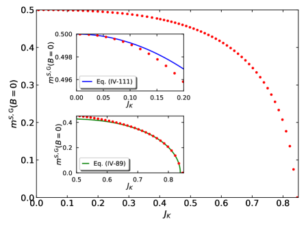
Figure 23: (Color online) Impurity spin polarization $m^{S,{\rm G}}(J_{\rm K})$ in the Gutzwiller wave function for the one-dimensional symmetric Kondo model as a function of $J_{\rm K}$ with the transition at $J_{\rm K,c}^{\rm G}\approx 0.839$. The mean-field behavior (IV-431) close to the transition and the expansion for small couplings (IV-453) are shown by straight lines.

IV.6.2 Expansion for small couplings

The numerical solution of the self-consistency equations for small couplings suggests the following behavior, using $V_{\uparrow}=V_{\downarrow}\equiv V$ and $\gamma_{\uparrow}=\gamma_{\downarrow}\equiv\gamma$

$$V \approx V_{1}J_{\rm K}+{\cal O}(J_{\rm K}^{2})\;,$$

$$\gamma \approx -\gamma_{1}J_{\rm K}+{\cal O}(J_{\rm K}^{2})\;,$$

$$E_{d} \approx E_{d,0}-E_{d,1}J_{\rm K}+{\cal O}(J_{\rm K}^{2})\;,$$

$$K \approx K_{1}J_{\rm K}+{\cal O}(J_{\rm K}^{2})\;,$$

$$m \approx \frac{1}{2}-m_{2}J_{\rm K}^{2}+{\cal O}(J_{\rm K}^{3})\;,$$

$$M_{0} \approx -M_{0,1}J_{\rm K}+{\cal O}(J_{\rm K}^{2})\;,$$

$$\omega_{p,\uparrow} : \hbox{no bound state}\;,$$

$$\omega_{p,\downarrow} \approx -1-\omega_{2}J_{\rm K}^{2}+{\cal O}(J_{\rm K}^{4})\;.$$ (IV-432)

Knowing that $E_{d}$ is of order unity, and $m\to 1/2$ for $J_{\rm K}\to 0$, we find from equation (IV.4) that

$$K=J_{\rm K}/4\;,$$ (IV-433)

so that $K_{1}=1/4$ in eq. (IV-432). Next, from eq. (LABEL:eq:Kderivativeband) we readily see that the band contribution to $M_{0}$ is proportional to $J_{\rm K}^{3}$ so that we are left with

$$\frac{\partial\omega_{p,\downarrow}}{\partial K}\approx\frac{(E_{d}+1)\left(-K(-1-E_{d})\right)}{(-1-E_{d})(-1)(-2-E_{d})-(-1-E_{d})}=-K$$ (IV-434)

to leading order in $J_{\rm K}$. Therefore, eq. (IV-410) gives

$$M_{0}=-\frac{K}{2}=-\frac{J_{\rm K}}{8}\;,$$ (IV-435)

so that $M_{0,1}=1/8$ in eq. (IV-432). As a consequence, $K(-1+E_{d})+V^{2}<0$ so that $\omega_{p,\uparrow}$ does not exist and

$$\omega_{p,\downarrow}=-1-\frac{K^{2}}{2}=-1-\frac{J_{\rm K}^{2}}{32}\;,$$ (IV-436)

so that $\omega_{2}=1/32$ in eq. (IV-432).

Eq. (IV-407) we then find

$$\gamma \approx V\int_{-1}^{0}\frac{{\rm d}\omega}{\pi}\frac{(E_{d}+\omega)\sqrt{1-\omega^{2}}}{(E_{d}+\omega)^{2}(1-\omega^{2})}\equiv VI_{1}(E_{d})\;,$$

$$I_{1}(E_{d}) = \int_{-1}^{0}\frac{{\rm d}\omega}{\pi}\frac{1}{(E_{d}+\omega)\sqrt{1-\omega^{2}}}$$ (IV-437)

$$= \frac{1}{\pi\sqrt{1-E_{d}^{2}}}\ln\left(\frac{E_{d}}{1+\sqrt{1-E_{d}^{2}}}\right)$$

for $0<E_{d}<1$. Moreover, eq. (IV-403) links $V$ and $\gamma$,

$$V=-\frac{J_{\rm K}}{\sqrt{1-4m^{2}}}\gamma\;,$$ (IV-438)

where we used that $m\to 1/2$ for $J_{\rm K}\to 0$. Therefore, we have obtained a first equation that relates $m$ and $E_{d}$. We have

$$\sqrt{1-4m^{2}}\approx\sqrt{4m_{2}}J_{\rm K}=-J_{\rm K}I_{1}(E_{d})\;,$$ (IV-439)

which implies

$$\sqrt{4m_{2}}=-I_{1}(E_{d})\quad,\quad m_{2}=\frac{I_{1}(E_{d})^{2}}{4}\;.$$ (IV-440)

In addition, from eq. (IV.4) we find

$$E_{d}\approx\frac{2}{(1-4m^{2})^{3/2}}J_{\rm K}\gamma^{2}=-2\left(\frac{\gamma}{J_{\rm K}}\right)^{2}\frac{1}{I_{1}(E_{d})^{3}}$$ (IV-441)

so that

$$\gamma = -J_{\rm K}\sqrt{\frac{E_{d}[-I_{1}(E_{d})]^{3}}{2}}\;,$$

$$V = J_{\rm K}\sqrt{\frac{-E_{d}I_{1}(E_{d})}{2}}$$ (IV-442)

are known as a function of $E_{d}$.

It remains to derive a second equation for $m_{2}$ as a function of $E_{d}$ from eq. (IV-418). There is no contribution from the bound states up to second order in $J_{\rm K}$, as seen from eq. (IV-436). The first non-negative contribution originates from

$$\frac{\partial E_{\uparrow}^{\rm band}(V_{\downarrow})}{\partial E_{d}}\approx\int_{-1}^{0}\frac{{\rm d}\omega}{\pi}\frac{V^{2}\sqrt{1-\omega^{2}}}{(\omega-E_{d})^{2}(1-\omega^{2})}=V^{2}I_{2}(E_{d})$$ (IV-443)

with

$$I_{2}(E_{d}) = \int_{-1}^{0}\frac{{\rm d}\omega}{\pi}\frac{1}{(\omega-E_{d})^{2}\sqrt{1-\omega^{2}}}$$

$$= \frac{1}{\pi E_{d}(1-E_{d}^{2})}$$

$$+\frac{E_{d}}{\pi(1-E_{d}^{2})^{3/2}}\ln\left(\frac{1-\sqrt{1-E_{d}^{2}}}{E_{d}}\right)$$

using Mathematica. Wolfram Research, Inc. (2016) In the remaining term we isolate the singularity for $V\to 0$,

$$\frac{\partial E_{\uparrow}^{\rm band}(V_{\uparrow})}{\partial E_{d}}\approx T_{a}(E_{d})+T_{b}(E_{d})\;,$$ (IV-445)

where

$$T_{a}(E_{d}) = -\int_{-1}^{0}\frac{{\rm d}\omega}{\pi}\sqrt{1-\omega^{2}}\frac{V^{2}}{(\omega+E_{d})^{2}(1-E_{d}^{2})+V^{4}}\;,$$

$$T_{b}(E_{d}) = \int_{-1}^{0}\frac{{\rm d}\omega}{\pi}\sqrt{1-\omega^{2}}\biggl{[}\frac{V^{2}}{(\omega+E_{d})^{2}(1-E_{d}^{2})+V^{4}}$$

$$-\frac{V^{2}}{(\omega+E_{d})^{2}(1-\omega^{2})+(V^{2}+K(\omega+E_{d}))^{2}}\biggr{]}\;.$$

Using Mathematica Wolfram Research, Inc. (2016) we find

$$T_{a}(x) = -1+V^{2}I_{3}(x)\;,$$

$$I_{3}(x) = \frac{2+\pi x}{2\pi x(1-x^{2})}$$ (IV-447)

$$+\frac{x}{\pi(1-x^{2})^{3/2}(\sqrt{1-x^{2}}+1)}\ln\biggl{(}\frac{1+\sqrt{1-x^{2}}}{x}\biggr{)}$$

$$+\frac{x}{2\pi(1-x^{2})(\sqrt{1-x^{2}}+1)}$$

$$\hphantom{+\;}\times\ln\biggl{(}\frac{2-x^{2}+2\sqrt{1-x^{2}}}{x^{2}}\biggr{)}\;.$$

In the term $T_{b}(E_{d})$ we are in the position to let $K,V\to 0$ in the denominator such that

$$T_{b}(x) \approx V^{2}\int_{-1}^{0}\frac{{\rm d}\omega}{\pi}\frac{\sqrt{1-\omega^{2}}}{(\omega+x)^{2}}\left[\frac{1}{(1-x^{2})}-\frac{1}{(1-\omega^{2})}\right]$$

$$= \frac{V^{2}}{1-x^{2}}\int_{-1}^{0}\frac{{\rm d}\omega}{\pi}\frac{1}{\sqrt{1-\omega^{2}}}\frac{x-\omega}{x+\omega}\equiv V^{2}I_{4}(x)\;,$$

$$I_{4}(x) = -\frac{1}{2(1-x^{2})}-\frac{2x}{\pi(1-x^{2})^{3/2}}\ln\biggl{(}\frac{1+\sqrt{1-x^{2}}}{x}\biggr{)}\,.$$

In total we find to second order in $V$ and thus in $J_{\rm K}$

$$m \approx \frac{1}{2}-\frac{V^{2}}{2}\left(I_{2}(E_{d})+I_{3}(E_{d})+I_{4}(E_{d})\right)$$

$$\approx \frac{1}{2}-J_{\rm K}^{2}\frac{E_{d}(-I_{1}(E_{d}))}{4}\left(I_{2}(E_{d})+I_{3}(E_{d})+I_{4}(E_{d})\right)$$

using eq. (IV-442) so that

$$m_{2} = \frac{E_{d}(-I_{1}(E_{d}))}{4}\left(I_{2}(E_{d})+I_{3}(E_{d})+I_{4}(E_{d})\right)$$ (IV-450)

$$\stackrel{{\scriptstyle!}}{{=}} \frac{I_{1}(E_{d})^{2}}{4}$$

from eq. (IV-440). The numerical solution of this equation gives

$$E_{d}=0.3857965059132358\;.$$ (IV-451)

Therefore, to leading order we have the analytic results,

$$V = \sqrt{\frac{-E_{d}I_{1}(E_{d})}{2}}J_{\rm K}+{\cal O}(J_{\rm K}^{2})\;,$$

$$= 0.32694495035854915J_{\rm K}+{\cal O}(J_{\rm K}^{2})\;,$$

$$\gamma = -\sqrt{\frac{E_{d}[-I_{1}(E_{d})]^{3}}{2}}J_{\rm K}+{\cal O}(J_{\rm K}^{2})\;,$$

$$= -0.18117388948693602J_{\rm K}+{\cal O}(J_{\rm K}^{2})\;,$$

and

$$E_{d} = 0.3857965059132358+{\cal O}(J_{\rm K})\;,$$

$$K = \frac{J_{\rm K}}{4}+{\cal O}(J_{\rm K}^{2})\;,$$

$$m = \frac{1}{2}-m_{2}J_{\rm K}^{2}+{\cal O}(J_{\rm K}^{3})\;,$$

$$m_{2} = \frac{I_{1}(E_{d})^{2}}{4}=0.07676830582531644\;,$$

$$M_{0} = -\frac{J_{\rm K}}{8}+{\cal O}(J_{\rm K}^{2})\;,$$

$$\omega_{p,\uparrow} : \hbox{no bound state}\;,$$

$$\omega_{p,\downarrow} = -1-\frac{J_{\rm K}^{2}}{32}+{\cal O}(J_{\rm K}^{4})\;.$$ (IV-453)

IV.6.3 Ground-state energy

The ground-state energy for small values of $J_{\rm K}$ must be determined numerically because the two integrals in eq. (IV-400) are too cumbersome to analyze in the weak-coupling limit. However, it can be shown that the Gutzwiller energy in eq. (229) is quadratic in the coupling for small $J_{\rm K}$. A quartic fit of the numerical data gives

$$E_{0}^{\rm G}(J_{\rm K})\approx-0.0908979J_{\rm K}^{2}-0.047363J_{\rm K}^{3}-0.0450817J_{\rm K}^{4}\;.$$ (IV-454)

The approximation is excellent up to $J_{\rm K}=0.4$. We may safely state that

$$E_{0}^{\rm G}(J_{\rm K})\approx-0.0905J_{\rm K}^{2}-0.051J_{\rm K}^{3}-0.05J_{\rm K}^{4}$$ (IV-455)

for the Gutzwiller variational energy for $J_{\rm K}\lesssim 0.4$. The quadratic coefficient can now be compared with the exact result from perturbation theory,

$$E_{0}(J_{\rm K})\approx-\frac{3}{32}J_{\rm K}^{2}=-0.09375J_{\rm K}^{2}\;.$$ (IV-456)

The magnetic Gutzwiller states accounts for 96.5% of the correlation energy.

Supplement V Ground-state energy from Bethe Ansatz

Using Bethe Ansatz, the Kondo model is solved for a linear dispersion relation with unit Fermi velocity in the wide-band limit, i.e., the dispersion relation $\epsilon^{\rm BA}(k)=k$ formally extends from $-\infty$ to $\infty$. Therefore, an appropriate energy cut-off $D$ must be introduced. This procedure is not unique. Therefore, there are two Bethe Ansatz solutions for the spin-1/2 Kondo model. First, the one discussed in Tsvelick and Wiegmann, Tsvelick and Wiegmann (1983) referred to as TW, and the one reviewed by Andrei, Furuya, and Lowenstein, Andrei et al. (1983) referred to as AFL. The basic Bethe Ansatz equations agree but the expressions for the parameters as a function of the Kondo coupling differ beyond leading-order in $J_{\rm K}^{\rm BA}/D$. For a lattice-regularized Bethe-Ansatz solvable impurity model, see Ref. [Bortz and Klümper, 2004].

V.1 Bethe Ansatz equations

V.1.1 Basic relations

According to equation (4.2.A) of TW, the electronic momenta are obtained from

$$e^{{\rm i}k_{j}L}=e^{-{\rm i}\phi}\prod_{\gamma=1}^{M}\frac{\tilde{\lambda}_{\gamma}+{\rm i}/2}{\tilde{\lambda}_{\gamma}-{\rm i}/2}\;,$$ (V-457)

where $L$ is a length scale that helps to quantize the momenta. $M=(N^{e}+1)/2$ in the ground state where $S^{z}=0$. The spin momenta are found from eq. (4.2.B) of TW,

$$\left[\frac{\tilde{\lambda}_{\gamma}+{\rm i}/2}{\tilde{\lambda}_{\gamma}-{\rm i}/2}\right]^{N^{e}}\left[\frac{\tilde{\lambda}_{\gamma}+1/g+{\rm i}/2}{\tilde{\lambda}_{\gamma}+1/g-{\rm i}/2}\right]=-\prod_{\delta=1}^{M}\left[\frac{\tilde{\lambda}_{\gamma}-\tilde{\lambda}_{\delta}+{\rm i}}{\tilde{\lambda}_{\gamma}-\tilde{\lambda}_{\delta}-{\rm i}}\right]$$ (V-458)

for $\gamma=1,\ldots,M$. Here, $g$ is the interaction parameter.

To make contact with the work by AFL, Andrei et al. (1983) we substitute

$$\tilde{\lambda}_{\gamma}=\frac{\lambda_{\gamma}-1}{g}$$ (V-459)

and set $g=c$ to find

$$e^{{\rm i}k_{j}L}=e^{-{\rm i}\phi}\prod_{\gamma=1}^{M}\frac{{\rm i}(1-\lambda_{\gamma})+c/2}{{\rm i}(1-\lambda_{\gamma})-c/2}$$ (V-460)

and $L(\lambda_{\gamma})=R(\lambda_{\gamma})$ with

$$L(\lambda_{\gamma}) = \left[\frac{{\rm i}(1-\lambda_{\gamma})+c/2}{{\rm i}(1-\lambda_{\gamma})-c/2}\right]^{N^{e}}\left[\frac{{\rm i}(-\lambda_{\gamma})+c/2}{{\rm i}(-\lambda_{\gamma})-c/2}\right]\;,$$

$$R(\lambda_{\gamma}) = -\prod_{\delta=1}^{M}\left[\frac{{\rm i}(\lambda_{\delta}-\lambda_{\gamma})+c}{{\rm i}(\lambda_{\delta}-\lambda_{\gamma})-c}\right]$$ (V-461)

for $\gamma=1,\ldots,M=(N^{e}+1)/2$. Eqs. (V-460) and (V-461) are eq. (2.47) and eq. (2.48’) of AFL. The energy is obtained from

$$E=\sum_{j=1}^{N^{e}}k_{j}\;,$$ (V-462)

see eq. (2.10’) of AFL and eq. (4.2.C) of TW.

Note that TW and AFL give different expressions for $\phi$ and $c$, namely

$$c^{\rm TW} = \tan(J_{\rm K}^{\rm BA})\approx J_{\rm K}^{\rm BA}+\frac{(J_{\rm K}^{\rm BA})^{3}}{3}+\ldots\;,$$ (V-463)

$$c^{\rm AFL} = \frac{J_{\rm K}^{\rm BA}}{1-3(J_{\rm K}^{\rm BA})^{2}/16}\approx J_{\rm K}^{\rm BA}+\frac{3}{16}(J_{\rm K}^{\rm BA})^{3}+\ldots\;,$$

and

$$\phi^{\rm TW} = -\frac{J_{\rm K}^{\rm BA}}{2}\;,$$

$$\phi^{\rm AFL} = {\rm i}\ln\left[\frac{1-3(J_{\rm K}^{\rm BA})^{2}/16+{\rm i}J_{\rm K}^{\rm BA}}{1+3(J_{\rm K}^{\rm BA})^{2}/16+{\rm i}J_{\rm K}^{\rm BA}/2}\right]$$ (V-464)

$$= {\rm i}\ln\left[\frac{4{\rm i}-J_{\rm K}^{\rm BA}}{4{\rm i}+J_{\rm K}^{\rm BA}}\right]$$

$$\approx -\frac{J_{\rm K}^{\rm BA}}{2}+\frac{(J_{\rm K}^{\rm BA})^{3}}{96}\;,$$

see eq. (4.2.A) and (4.2.55’) of TW with $I\equiv 2J_{\rm K}^{\rm BA}$ and eq. (2.42) of AFT, where $J=-J^{\prime\prime}=J_{\rm K}^{\rm BA}/2$ was used. To leading order, the interaction parameters agree but they differ to third order in $J_{\rm K}^{\rm BA}$. As a consequence, the ground-state energy agrees to leading order in $J_{\rm K}^{\rm BA}$ only.

V.1.2 Non-interacting case

We can take the limit $c\to 0^{+}$ in eqs. (V-460) and (V-461) because the parameters $\lambda_{\gamma}$ remain finite in the non-interacting limit, see below. Therefore, we find that eq. (V-461) is fulfilled if we assume that all $\lambda_{\gamma}$ are pairwise different and different from zero. This is fulfilled for finite system sizes. Moreover, eq. (V-460) reduces to

$$e^{{\rm i}k_{j}^{(0)}L}=1$$ (V-465)

because $\phi(0)=0$ so that

$$k_{j}^{(0)}=\frac{2\pi}{L}\tilde{n}_{j}$$ (V-466)

with integer $\tilde{n}_{j}$ and

$$E^{\rm(0),BA}=\frac{2\pi}{L}\sum_{j=1}^{N^{e}}\tilde{n}_{j}\;.$$ (V-467)

In the following, we are interested in the ground state and its energy in the thermodynamic limit.

We want to make contact with our lattice Hamiltonian. Its dispersion around the Fermi wave vector is linear,

$$\epsilon(m)\approx 2t\frac{2\pi(m-m_{\rm F})}{L+1}\;.$$ (V-468)

When we work with a half-filled band, $N^{e}=(L+3)/2\approx L/2$, the corrections to the linear dispersion relation are not of second order, but of order $(m-m_{\rm F})^{3}$, see eq. (165). Therefore, the Bethe Ansatz results agree with those from DMRG for the lattice Hamiltonian in a larger region of $J_{\rm K}$-values. For $t=1/2$ and $m_{\rm F}=(L+3)/4\approx L/4$ ($L\gg 1$) we have

$$E_{0}^{\rm(0),latt}=2(2t)\frac{2\pi}{L}\sum_{m=1}^{m_{\rm F}}(m-m_{\rm F})=-\frac{\pi L}{8}\;,$$ (V-469)

where the additional factor two accounts for the spin degeneracy.

Therefore, in eq. (V-467) we choose the $N^{e}\approx L/2$ integers

$$\tilde{n}_{j}=-\frac{3N^{e}}{4},\ldots,\frac{N^{e}}{4}-1$$ (V-470)

for our sequence of Bethe-Ansatz charge quantum numbers. Then,

$$E_{0}^{\rm(0),BA}=\frac{2\pi}{L}\sum_{\tilde{n}=-3N^{e}/4}^{N^{e}/4-1}\tilde{n}=-\frac{\pi L}{8}\;,$$ (V-471)

in agreement with the expression (V-469) for the lattice Hamiltonian $E_{0}^{\rm(0),BA}=E_{0}^{\rm(0),latt}$.

V.1.3 Energy from Bethe quantum numbers

We use the following identity,

$$\ln\left[\frac{{\rm i}x+1}{{\rm i}x-1}\right]=(-2{\rm i}){\rm arccot}(x)\;.$$ (V-472)

Note that ${\rm arccot}(x)$ has a jump discontinuity of $-\pi$ at $x=0$.

Therefore, taking the complex logarithm of eqs. (V-460) gives

$${\rm i}k_{j}L=2\pi{\rm i}\tilde{n}_{j}-{\rm i}\phi+(-2{\rm i})\sum_{\gamma=1}^{(N^{e}+1)/2}{\rm arccot}\left[2(1-\lambda_{\gamma})/c\right]\;.$$ (V-473)

The integer numbers $\tilde{n}_{j}$ (charge Bethe quantum numbers) distinguish between the various electron momenta.

The energy (V-462) thus becomes

$$E = \sum_{j=1}^{N^{e}}\frac{2\pi}{L}\tilde{n}_{j}-\frac{N^{e}}{L}\phi$$

$$+\frac{N^{e}}{L}\sum_{\gamma=1}^{(N^{e}+1)/2}\left(-2{\rm arccot}\left[2(1-\lambda_{\gamma})/c\right]\right)\;.$$

Eq. (LABEL:eq:BA31corrected) replaces eq. (3.1) of AFL where the $\phi$-term was dropped as ‘inessential’. Of course, it is important for the complete ground-state energy.

Next, taking the complex logarithm of eq. (V-461) we find

$$L(\lambda_{\gamma}) = R(\lambda_{\gamma})\;,$$

$$L(\lambda_{\gamma}) = N^{e}\left(-2{\rm arccot}\left[2(1-\lambda_{\gamma})/c\right]\right)$$

$$+\left(-2{\rm arccot}\left[2(-\lambda_{\gamma})/c\right]\right)\;,$$

$$R(\lambda_{\gamma}) = 2\pi\tilde{I}_{\gamma}+\sum_{\delta=1}^{(N^{e}+1)/2}\left(-2{\rm arccot}\left[(\lambda_{\delta}-\lambda_{\gamma})/c\right]\right)\;,$$

where the $(N^{e}+1)/2$ (half-)integer numbers $\tilde{I}_{\gamma}$ (spin Bethe quantum numbers) distinguish the various spin momenta.

V.1.4 Contact with energy formulae in AFL

In our formulae (LABEL:eq:BA31corrected) and (LABEL:eq:improved32) we replace

$$-2{\rm arccot}(-x)=-2\arctan(x)-\pi+2\pi\theta_{\rm H}(x)\;,$$ (V-476)

where $\theta_{\rm H}(x)$ is the Heaviside step function. We define

$$\Theta(x)=-2\arctan(x/c)$$ (V-477)

to make close contact with the formulae in AFL. Then, eq. (LABEL:eq:BA31corrected) becomes

$$E=\sum_{j=1}^{N^{e}}\frac{2\pi}{L}n_{j}-\frac{N^{e}}{L}\phi+\frac{N^{e}}{L}\sum_{\gamma=1}^{(N^{e}+1)/2}\left[\Theta\left(2\lambda_{\gamma}-2\right)-\pi\right]\;,$$ (V-478)

where we set

$$n_{j}=\tilde{n}_{j}+\sum_{\gamma=1}^{(N^{e}+1)/2}\theta_{H}\left((2\lambda_{\gamma}-2)/c\right)\;.$$ (V-479)

Apart from the $\phi$-term, eq. (V-478) is eq. (3.1) of AFL.

Furthermore, eq. (LABEL:eq:improved32) becomes

$$N^{e}\Theta_{\rm H}(2\lambda_{\gamma}-2)+\Theta(2\lambda_{\gamma})=-2\pi I_{\gamma}+\sum_{\delta=1}^{(N^{e}+1)/2}\Theta(\lambda_{\gamma}-\lambda_{\delta})$$ (V-480)

with a proper re-definition of the (half-)integers $I_{\gamma}$. Eq. (V-480) is eq. (3.2) of AFL.

V.2 Spin distribution function

V.2.1 Integral equation for the spin momenta

We start from eq. (V-480) and define the spin distribution function

$$\sigma(\lambda_{\gamma})=\frac{1}{\lambda_{\gamma+1}-\lambda_{\gamma}}=\frac{1}{\Delta\lambda_{\gamma}}\;,$$ (V-481)

which is of the order $1/L$ for $L\gg 1$. As usual, we take the difference of two consecutive values for $\gamma$,

$$-2\pi = -2\pi I_{\gamma+1}+2\pi I_{\gamma}$$

$$= N^{e}\left[\Theta(2\lambda_{\gamma+1}-2)-\Theta(2\lambda_{\gamma}-2)\right]$$

$$+\Theta(2\lambda_{\gamma+1})-\Theta(2\lambda_{\gamma})$$

$$-\int{\rm d}\lambda^{\prime}\sigma(\lambda^{\prime})\left[\Theta(\lambda_{\gamma+1}-\lambda^{\prime})-\Theta(\lambda_{\gamma}-\lambda^{\prime})\right]\;,$$

where we used the definition of the Riemann integral in the thermodynamic limit,

$$\sum_{\delta}f(\lambda_{\delta})=\int\frac{{\rm d}\lambda^{\prime}}{\Delta\lambda^{\prime}}f(\lambda^{\prime})=\int{\rm d}\lambda^{\prime}\sigma(\lambda^{\prime})f(\lambda^{\prime})\;.$$ (V-483)

Using eq. (V-481) again we find

$$\Theta(2\lambda_{\gamma+1}-2)-\Theta(2\lambda_{\gamma}-2)=\Theta^{\prime}(2\lambda_{\gamma}-2)\frac{2}{\sigma(\lambda_{\gamma})}$$ (V-484)

with

$$\Theta^{\prime}(x)=-\frac{2c}{x^{2}+c^{2}}\;.$$ (V-485)

Thus, eq. (LABEL:eq:intermediate) becomes by setting $\lambda_{\gamma}\equiv\lambda$

$$-2\pi\sigma(\lambda) = 2N^{e}\Theta^{\prime}(2\lambda-2)+2\Theta^{\prime}(2\lambda)$$ (V-486)

$$-\int{\rm d}\lambda^{\prime}\sigma(\lambda^{\prime})\Theta^{\prime}(\lambda-\lambda^{\prime})\;.$$

This is the integral equation (3.8) of AFL,

$$\sigma(\lambda)=f(\lambda)-\int{\rm d}\lambda^{\prime}K(\lambda-\lambda^{\prime})\sigma(\lambda^{\prime})$$ (V-487)

with

$$f(\lambda) = \frac{2c}{\pi}\left(\frac{N^{e}}{c^{2}+4(\lambda-1)^{2}}+\frac{1}{c^{2}+4\lambda^{2}}\right)\;,$$

$$K(\lambda) = \frac{c}{\pi}\frac{1}{c^{2}+\lambda^{2}}\;\;,$$ (V-488)

in agreement with eq. (3.9) of AFL.

V.2.2 Solution of the integral equation

Upon Fourier transformation

$$g(\lambda) = \int{\rm d}xg(x)e^{{\rm i}\lambda x}\;,$$

$$g(x) = \int\frac{{\rm d}\lambda}{2\pi}g(\lambda)e^{-{\rm i}\lambda x}\;,$$ (V-489)

we obtain from eq. (V-487)

$$\sigma(x)=\frac{f(x)}{1+K(x)}$$ (V-490)

with

$$f(x) = \int{\rm d}\lambda e^{{\rm i}\lambda x}\frac{2c}{\pi}\left(\frac{N^{e}}{c^{2}+4(\lambda-1)^{2}}+\frac{1}{c^{2}+4\lambda^{2}}\right)$$ (V-491)

$$= e^{-c|x|/2}\left(N^{e}e^{{\rm i}x}+1\right),$$

$$K(x) = \int{\rm d}\lambda e^{{\rm i}\lambda x}\frac{c}{\pi}\frac{1}{c^{2}+\lambda^{2}}=e^{-c|x|}\;.$$ (V-492)

Therefore, we obtain $\sigma(\lambda)$ from eq. (V-489) and eq. (V-490) as

$$\sigma(\lambda) = \int\frac{{\rm d}x}{2\pi}e^{-{\rm i}\lambda x-c|x|/2}\frac{N^{e}e^{{\rm i}x}+1}{1+e^{-c|x|}}$$

$$= \int\frac{{\rm d}x}{2\pi}\frac{e^{-{\rm i}\lambda x}}{2\cosh(cx/2)}\left(N^{e}e^{{\rm i}x}+1\right)$$

$$= \frac{1}{2c}\left(\frac{N^{e}}{\cosh(\pi(\lambda-1)/c)}+\frac{1}{\cosh(\pi\lambda/c)}\right)\;,$$

using Mathematica. Wolfram Research, Inc. (2016) Eq. (LABEL:eq:310) is eq. (3.10) of AFL.

V.3 Ground-state energy

V.3.1 Charge quantum numbers in the ground state

In eq. (V-470) we determined the values for the charge Bethe-Ansatz quantum numbers $\tilde{n}_{j}$ in the ground state. According to eq. (V-479), the quantum numbers $n_{j}$ obey

$$n_{j} = \tilde{n}_{j}+\int{\rm d}\lambda\sigma(\lambda)\theta_{\rm H}((2\lambda-2)/c)$$ (V-494)

$$= \tilde{n}_{j}+\frac{N^{e}}{2c}\int_{1}^{\infty}{\rm d}\mu\frac{1}{\cosh(\pi\mu/c)}$$

$$= \tilde{n}_{j}+\frac{N^{e}}{4}$$

in the thermodynamic limit. Consequently, we find from eq. (V-470) that the quantum numbers $n_{j}$ are symmetrically distributed around zero,

$$n_{j}=-\frac{N^{e}}{2},\ldots,\frac{N^{e}}{2}-1\;.$$ (V-495)

as discussed in TW, Sect. 5.1.1.

V.3.2 Ground-state energy in the thermodynamic limit

In the thermodynamic limit, the ground-state energy in eq. (V-478) becomes

$$E_{0} = -\frac{N^{e}}{L}\phi+\frac{N^{e}}{L}\int{\rm d}\lambda\sigma(\lambda)\left[\Theta(2\lambda-2)-\pi\right]$$ (V-496)

$$\equiv \frac{N^{e}}{L}\left(-\phi+{\cal B}(c)+{\cal I}(c)\right)\;,$$

because the quantum numbers $n_{j}$ are distributed symmetrically around zero so that the sum over all occupied $n_{j}$ gives zero. Here,

$${\cal B}(c) \equiv \int{\rm d}\lambda\frac{N^{e}}{2c}\frac{\Bigl{[}-\pi-2\arctan\left[2(\lambda-1)/c\right]\Bigr{]}}{\cosh(\pi(\lambda-1)/c)}$$ (V-497)

$$= -\frac{\pi}{2}N^{e}\;,$$

and

$${\cal I}(c) = {\cal I}_{1}(c)+{\cal I}_{2}(c)\;,$$

$${\cal I}_{1}(c) = -\pi\int_{-\infty}^{\infty}{\rm d}\lambda\frac{1}{2c\cosh[\pi\lambda/c]}=-\frac{\pi}{2}\;,$$ (V-498)

$${\cal I}_{2}(c) = \int_{-\infty}^{\infty}{\rm d}\lambda\frac{1}{2c\cosh[\pi\lambda/c]}\Bigl{[}-2\arctan\left[2(\lambda-1)/c\right]\Bigr{]}\;.$$

Altogether, we have

$$E_{0}=-\frac{\pi(N^{e})^{2}}{2L}+\frac{N^{e}}{L}\left(-\phi-\frac{\pi}{2}+{\cal I}_{2}(c)\right)\;.$$ (V-500)

Apart from the $\phi$-term this is the first line of eq. (3.12) of AFL.

When we subtract the energy $E_{0}^{\rm(0),BA}$ for $c=0$, see eq. (V-471), we find

$$e_{0}(J)=E_{0}-E_{0}^{(0),{\rm BA}}=\frac{1}{2}\left(-\phi-\frac{\pi}{2}+{\cal I}_{2}(c)\right)\;,$$ (V-501)

where we used $N^{e}=L/2$.

V.3.3 Evaluation of the integral ${\cal I}_{2}(c)$

The calculation of the ground-state energy requires the evaluation of the integral ${\cal I}_{2}(c)$, eq. (LABEL:eq;startIc). For its calculation we use the integral representation of the arctan function

$$\arctan(\lambda)=\int_{0}^{\infty}{\rm d}\omega e^{-\omega}\frac{\sin(\omega\lambda)}{\omega}$$ (V-502)

to find

$${\cal I}_{2}(c)=-\frac{1}{c}\int_{0}^{\infty}\frac{{\rm d}\omega}{\omega}e^{-\omega}\int_{-\infty}^{\infty}{\rm d}\lambda\frac{\sin\left(2\omega(\lambda-1)/c\right)}{\cosh(\pi\lambda/c)}\;.$$ (V-503)

With the help of Mathematica Wolfram Research, Inc. (2016) we can write ${\cal I}_{2}(c)$ as

$${\cal I}_{2}(c)=\int_{0}^{\infty}\frac{{\rm d}\omega}{\omega}e^{-\omega}\frac{\sin(2\omega/c)}{\cosh\omega}=\int_{-\infty}^{\infty}\frac{{\rm d}\omega}{{\rm i}\omega}\frac{e^{{\rm i}\omega}}{e^{|\omega|c}+1}\;.$$ (V-504)

The latter integral can be found in eq. (17.18) in Ref. [Essler et al., 2010]

$${\cal I}_{2}(c)={\rm i}\ln\left[\frac{\displaystyle\Gamma\left(\frac{1}{2}+\frac{{\rm i}}{2c}\right)\Gamma\left(1-\frac{{\rm i}}{2c}\right)}{\displaystyle\Gamma\left(\frac{1}{2}-\frac{{\rm i}}{2c}\right)\Gamma\left(1+\frac{{\rm i}}{2c}\right)}\right]\;.$$ (V-505)

It can be derived using the series expansion of $1/\cosh(\omega)$, performing the $\omega$-integral, and using eq. (6.3.13) of [Abramowitz and Stegun, 1964]. Eqs. (V-501) and (V-505) correct the typographical errors in equation (3.12) of AFL.

V.3.4 Final result for the ground-state energy

Lastly, we summarize the result for the ground-state energy from Bethe Ansatz that originates from the interaction of the impurity spin and the bath spin at the origin.

Andrei, Furuya, Lowenstein

$$e_{0}^{\rm AFL}(J) = \arctan(J/2)+\frac{1}{2}\left(-\frac{\pi}{2}+{\cal I}_{2}(c)\right)\;,$$

$$c^{\rm AFL} = \frac{2J}{1-3J^{2}/4}\;,$$

$${\cal I}_{2}(c) = {\rm i}\ln\left[\frac{\displaystyle\Gamma\left(\frac{1}{2}+\frac{{\rm i}}{2c}\right)\Gamma\left(1-\frac{{\rm i}}{2c}\right)}{\displaystyle\Gamma\left(\frac{1}{2}-\frac{{\rm i}}{2c}\right)\Gamma\left(1+\frac{{\rm i}}{2c}\right)}\right]$$ (V-506)

with $J=J_{\rm K}^{\rm BA}/2$. The expansion for small couplings $J$ reads

$$e_{0}^{\rm AFL}(J) = \frac{J}{2}-\frac{J^{3}}{24}+\frac{J^{5}}{160}-\frac{1}{2}\left(\frac{c}{2}+\frac{c^{3}}{12}+\frac{c^{5}}{10}\right)$$ (V-507)

$$= \frac{J}{2}-\frac{J^{3}}{24}+\frac{J^{5}}{160}-\left(\frac{J}{2}+\frac{17J^{3}}{24}+\frac{421J^{5}}{160}\right)$$

$$= -\frac{3J^{3}}{4}-\frac{21J^{5}}{8}$$

$$= -\frac{3}{32}(J_{\rm K}^{\rm BA})^{3}-\frac{21}{256}(J_{\rm K}^{\rm BA})^{5}\;,$$

up to corrections of the order $(J_{\rm K}^{\rm BA})^{7}$. The result was obtained using Mathematica. Wolfram Research, Inc. (2016)

Tsvelick and Wiegmann

$$e_{0}^{\rm TW}(I) = \frac{I}{8}+\frac{1}{2}\left(-\frac{\pi}{2}+{\cal I}_{2}(c)\right)\;,$$

$$c^{\rm TW} = \tan(I/2)\;,$$

$${\cal I}_{2}(c) = {\rm i}\ln\left[\frac{\displaystyle\Gamma\left(\frac{1}{2}+\frac{{\rm i}}{2c}\right)\Gamma\left(1-\frac{{\rm i}}{2c}\right)}{\displaystyle\Gamma\left(\frac{1}{2}-\frac{{\rm i}}{2c}\right)\Gamma\left(1+\frac{{\rm i}}{2c}\right)}\right]$$ (V-508)

with $I=2J_{\rm K}^{\rm BA}$. The expansion for small couplings $I$ reads

$$e_{0}^{\rm TW}(I) = \frac{I}{8}-\frac{1}{2}\left(\frac{c}{2}+\frac{c^{3}}{12}+\frac{c^{5}}{10}\right)$$ (V-509)

$$= \frac{I}{8}-\left(\frac{I}{8}+\frac{I^{3}}{64}+\frac{I^{5}}{256}\right)=-\frac{I^{3}}{64}-\frac{I^{5}}{256}$$

$$= -\frac{4}{32}(J_{\rm K}^{\rm BA})^{3}-\frac{32}{256}(J_{\rm K}^{\rm BA})^{5}\;,$$

up to corrections of the order $(J_{\rm K}^{\rm BA})^{7}$. The result was obtained using Mathematica. Wolfram Research, Inc. (2016)

The comparison of eq (V-507) and (V-509) show that the two expressions differ to third order. More importantly, neither of the approaches contains a second-order term, see eq. (34). Consequently, the Bethe Ansatz results for the ground-state energy only apply to first order in $J_{\rm K}/W$, as is implicit in the wide-band limit, $W\to\infty$.

V.4 Two-particle problem

It is instructive to solve the two-particle problem. We address a linear dispersion relation.

V.4.1 Analytic solution

We focus on the subspace that contains the ground state, $S=S^{z}=0$. We thus investigate the $(L+1)/2$ normalized states

$$|m\rangle=\sqrt{\frac{1}{2}}\left(\hat{b}_{m,\uparrow}^{+}\hat{d}_{\downarrow}^{+}-\hat{b}_{m,\downarrow}^{+}\hat{d}_{\uparrow}^{+}\right)|\hbox{vac}\rangle\;,$$ (V-510)

where $\hat{b}_{m,\sigma}^{+}$ creates an electron in the kinetic-energy eigenstate of the half-chain with energy $\epsilon(m)$,

$$\langle m|\hat{T}^{C}|m^{\prime}\rangle=\delta_{m,m^{\prime}}\epsilon(m)\;.$$ (V-511)

In the spin-singlet basis $|m\rangle$, the Kondo coupling reduces to an attractive potential scattering term,

$$\langle m|\hat{V}_{\rm sd}|m^{\prime}\rangle=-\frac{3J_{\rm K}}{4}\frac{2}{L+1}(-1)^{m+m^{\prime}}\;.$$ (V-512)

We solve the Schrödinger equation

$$\left(\hat{T}^{C}+\hat{V}_{\rm sd}\right)|\psi\rangle=E|\psi\rangle$$ (V-513)

with the Ansatz

$$|\psi\rangle=\sum_{r=1}^{(L+1)/2}(-1)^{r}f_{r}|r\rangle$$ (V-514)

and find

$$\left(E-\epsilon(r)\right)f_{r}=\frac{3J_{\rm K}}{2(L+1)}\sum_{m=1}^{(L+1)/2}f_{m}\;,$$ (V-515)

which has the solution

$$f_{r}=-\frac{3J_{\rm K}}{4}\frac{\gamma(E)}{E-\epsilon(r)}\;,$$ (V-516)

where $\gamma(E)$ follows from the solution of

$$1=-\frac{3J_{\rm K}}{4}\frac{2}{L+1}\sum_{r=1}^{(L+1)/2}\frac{1}{E-\epsilon(r)}\;.$$ (V-517)

This equation has a simple solution for $J_{\rm K}\gg 1$, because we can replace the sum by $(L+1)/(2E)$ so that $E(J_{\rm K}\gg 1)=-3J_{\rm K}/4$. For strong coupling, a local singlet forms between the impurity spin and the bath spin on site $n=0$. The analysis of the weak-coupling limit is more subtle.

Finite system sizes

As long as $L$ is finite, there are no bound states, and we can set

$$E_{0}=\epsilon(1)-\frac{\delta}{L+1}\;,$$ (V-518)

where $\delta>0$ is of the order unity. Furthermore, we use

$$\epsilon(m)=\frac{2\pi}{L+1}\left(m-\frac{(L+3)}{4}\right)$$ (V-519)

for our half-chain Hamiltonian. Then, eq. (V-517) becomes

$$\delta=\frac{3J_{\rm K}}{2}\left(1+\frac{\delta}{2\pi}\sum_{r=1}^{(L-1)/2}\frac{1}{r+\delta/(2\pi)}\right)\;.$$ (V-520)

Apparently, this equation has the solution $\delta=3J_{\rm K}/2$ for small $J_{\rm K}$ so that

$$e_{0}(J_{\rm K})=E_{0}-\epsilon(1)=-\frac{1}{L+1}\frac{3J_{\rm K}}{2}+{\cal O}\left(J_{\rm K}^{2}\ln(L)/L\right)$$ (V-521)

for $J_{\rm K}\ll 1/\ln(L)$. For finite system sizes, the energy is linear in $J_{\rm K}$ but the prefactor is proportional to $1/L$ so that the linear term vanishes in the thermodynamic limit. Moreover, the linear region itself vanishes logarithmically for large system sizes.

Thermodynamic limit

The sum in eq. (V-520) diverges logarithmically. Therefore, we must use that

$$e_{0}=E_{0}-\epsilon(1)$$ (V-522)

is finite in the thermodynamic limit. Then, eq. (V-517) becomes

$$1=\frac{3J_{\rm K}}{4}\frac{2}{L}\frac{L}{2\pi}\int_{0}^{\pi}{\rm d}k\frac{1}{-e_{0}+k}=\frac{3J_{\rm K}}{4\pi}\ln\left[\frac{-e_{0}+\pi}{(-e_{0})}\right]$$ (V-523)

so that

$$e_{0}(J_{\rm K})=-\frac{\pi}{\exp\left(4\pi/(3J_{\rm K})\right)-1}\;.$$ (V-524)

Therefore, $e_{0}(J_{\rm K})$ is exponentially small but finite in the thermodynamic limit. This does not come as a surprise because attractive potentials support bound states in one-dimensional scattering problems. For large $J_{\rm K}$ we recover eq. (V-521).

V.4.2 Bethe Ansatz

We analyze the Bethe Ansatz equation for finite $L$ because we can then assure that there are no bound states. For $N^{e}=1$ we find from eq. (V-461) for $M=1$

$$\left[\frac{{\rm i}(1-\lambda)+c/2}{{\rm i}(1-\lambda)-c/2}\right]\left[\frac{{\rm i}(-\lambda)+c/2}{{\rm i}(-\lambda)-c/2}\right]=(-1)(-1)\;,$$ (V-525)

which has the solution $\lambda=1/2$. The energy becomes

$$E_{0}=\frac{2\pi}{L}\tilde{n}_{1}-\frac{\phi}{L}-\frac{2}{L}\arctan(c)$$ (V-526)

or

$$e_{0}=-\frac{1}{L}\left(\phi+2\arctan(c)\right)\;.$$ (V-527)

For the two Bethe Ansatz expression we obtain the following results.

Andrei, Furuya, Lowenstein.

Eq. (V-463) together with eq. (V-464) gives

$$e_{0}^{\rm AFL}(J_{\rm K}^{\rm BA}) = \frac{2}{L}\arctan\left(\frac{J_{\rm K}^{\rm BA}}{4}\right)$$ (V-528)

$$-\frac{2}{L}\arctan\left(\frac{J_{\rm K}^{\rm BA}}{1-3(J_{\rm K}^{\rm BA})^{2}/16}\right)$$

$$= -\frac{1}{L}\left(\frac{3J_{\rm K}^{\rm BA}}{2}-\frac{9(J_{\rm K}^{\rm BA})^{3}}{32}\right)\;,$$

and corrections are of the order $(J_{\rm K}^{\rm BA})^{5}$. Note that the solution with a finite bandwidth, eq. (V-521), has $L$-dependent corrections of the order $J_{\rm K}^{2}\ln(L)/L$ for $J_{\rm K}\ll 1/\ln(L)$.

Tsvelick and Wiegmann.

Eq. (V-463) together with eq. (V-464) gives

$$e_{0}^{\rm TW}(J_{\rm K}^{\rm BA})=-\frac{1}{L}\frac{3J_{\rm K}^{\rm BA}}{2}$$ (V-529)

without corrections to higher orders in $J_{\rm K}^{\rm BA}$, in agreement with eq. (V-521).

The agreement between eq. (V-521) and eq. (V-529) can be improved when a flexible the length scale is used in Bethe Ansatz, $L^{\rm BA}\sim L\ln(L)$, instead of $L^{\rm BA}=L$. We shall not further elaborate this possibility.

Supplement VI Free energy in second-order weak-coupling perturbation theory

For a better comparison, we closely follow the considerations in appendix C of AFL.

VI.1 Formal expansion

The unperturbed Hamiltonian is defined by

$$\hat{H}_{0}=\hat{T}+\hat{H}_{\rm mag}\;.$$ (VI-530)

In perturbation theory we need the Kondo term in the interaction picture,

$$\hat{V}_{\rm sd}(\lambda)=e^{\lambda\hat{H}_{0}}\hat{V}_{\rm sd}e^{-\lambda\hat{H}_{0}}\;.$$ (VI-531)

We use

$$e^{\lambda\hat{H}_{0}}\hat{b}_{k,\uparrow}^{+}e^{-\lambda\hat{H}_{0}} = e^{(\epsilon(k)-B)\lambda}\hat{b}_{k,\uparrow}^{+}\;,$$

$$e^{\lambda\hat{H}_{0}}\hat{b}_{k,\downarrow}^{+}e^{-\lambda\hat{H}_{0}} = e^{(\epsilon(k)+B)\lambda}\hat{b}_{k,\downarrow}^{+}\;,$$

$$e^{\lambda\hat{H}_{0}}\hat{d}_{\uparrow}^{+}e^{-\lambda\hat{H}_{0}} = e^{-B\lambda}\hat{d}_{\uparrow}^{+}\;,$$

$$e^{\lambda\hat{H}_{0}}\hat{d}_{\downarrow}^{+}e^{-\lambda\hat{H}_{0}} = e^{B\lambda}\hat{d}_{\downarrow}^{+}\;.$$ (VI-532)

Therefore,

$$\hat{V}_{\rm sd}(\lambda) = \frac{J_{\rm K}}{L}\sum_{k,k^{\prime}}e^{(\epsilon(k^{\prime})-\epsilon(k))\lambda}$$

$$\times\Bigl{[}\hat{b}_{k^{\prime},\uparrow}^{+}\hat{b}_{k,\downarrow}^{\vphantom{+}}\hat{d}_{\downarrow}^{+}\hat{d}_{\uparrow}^{\vphantom{+}}+\hat{b}_{k^{\prime},\downarrow}^{+}\hat{b}_{k,\uparrow}^{\vphantom{+}}\hat{d}_{\uparrow}^{+}\hat{d}_{\downarrow}^{\vphantom{+}}$$

$$\hphantom{\times\Bigl{[}}+\frac{1}{2}(\hat{d}_{\uparrow}^{+}\hat{d}_{\uparrow}^{\vphantom{+}}-\hat{d}_{\downarrow}^{+}\hat{d}_{\downarrow}^{\vphantom{+}})(\hat{b}_{k^{\prime},\uparrow}^{+}\hat{b}_{k,\uparrow}^{\vphantom{+}}-\hat{b}_{k^{\prime},\downarrow}^{+}\hat{b}_{k,\downarrow}^{\vphantom{+}})\Bigr{]}\;,$$

as in eq. (C6) of AFL.

The partition function contains the terms

$$Z_{0} = \hbox{Tr}\left(e^{-\beta\hat{H}_{0}}\right)\;,$$

$$Z_{1} = -\hbox{Tr}\left(e^{-\beta\hat{H}_{0}}\int_{0}^{\beta}{\rm d}\lambda\hat{V}_{\rm sd}(\lambda)\right)\;,$$

$$Z_{2} = \hbox{Tr}\left(e^{-\beta\hat{H}_{0}}\int_{0}^{\beta}{\rm d}\lambda_{1}\hat{V}_{\rm sd}(\lambda_{1})\int_{0}^{\lambda_{1}}{\rm d}\lambda_{2}\hat{V}_{\rm sd}(\lambda_{2})\right)\;,$$

see eq. (C5) of AFL, where $\beta=1/T$ is the inverse temperature. The free energy ${\cal F}=-T\ln(Z)$ becomes

$${\cal F}=-T\left[\ln(Z_{0})+\frac{Z_{1}}{Z_{0}}+\frac{Z_{2}}{Z_{0}}-\frac{1}{2}\left(\frac{Z_{1}}{Z_{0}}\right)^{2}\right]\;,$$ (VI-535)

up to and including second order in $J_{\rm K}$, see eq. (C7) of AFL.

VI.2 Terms up to first order

The leading-order term in the impurity-induced contribution to free energy is obtained from

$$Z_{0}^{\rm ii}=e^{\beta B}+e^{-\beta B}=2\cosh(\beta B)$$ (VI-536)

as

$${\cal F}_{0}^{\rm ii}=-T\ln[2\cosh(\beta B)]\;.$$ (VI-537)

From the definition (LABEL:eq:defineorders) we find for the first-order term

$$Z_{1} = -J_{\rm K}\frac{1}{L}\sum_{k,k^{\prime}}\int_{0}^{\beta}{\rm d}\lambda e^{\lambda(\epsilon(k^{\prime})-\epsilon(k))}$$

$$\times\hbox{Tr}\left(e^{-\beta\hat{H}_{0}}\frac{1}{2}(\hat{d}_{\uparrow}^{+}\hat{d}_{\uparrow}^{\vphantom{+}}-\hat{d}_{\downarrow}^{+}\hat{d}_{\downarrow}^{\vphantom{+}})(\hat{b}_{k^{\prime},\uparrow}^{+}\hat{b}_{k,\uparrow}^{\vphantom{+}}-\hat{b}_{k^{\prime},\downarrow}^{+}\hat{b}_{k,\downarrow}^{\vphantom{+}})\right)$$

because the spin-flip terms do not contribute as the trace is done over states with fixed $d$-occupation. The impurity trace gives

$$F(B/T)\equiv\frac{Z_{1}^{\rm i}}{Z_{0}^{\rm i}}=\frac{\hbox{Tr}\left(e^{2\beta B\hat{S}_{z}}\hat{S_{z}}\right)}{\hbox{Tr}\left(e^{2\beta B\hat{S}_{z}}\right)}=\frac{1}{2}\tanh(\beta B)\;,$$ (VI-539)

see eq. (C15) of AFL. The host-electron trace is trivial because only $k=k^{\prime}$ can contribute,

$$\frac{Z_{1}^{\rm e}}{Z_{0}^{\rm e}}\equiv\frac{1}{2}\frac{N_{\uparrow}-N_{\downarrow}}{L/2}\equiv M\;.$$ (VI-540)

In the presence of a magnetic field, the host-electrons have the magnetization

$$M = \frac{B}{\pi}\quad\hbox{for}\quad\epsilon(k)=k\;,$$

$$M = \frac{\arcsin(B)}{\pi}\quad\hbox{for}\quad\epsilon(k)=\sin(k)\;.$$ (VI-541)

We may safely assume that, for $J_{\rm K}\ll 1$, the external field is weak enough to only slightly polarize the host-electron system. When we work with a general density of states and small fields, we find $M=B\rho_{0}(0)$ for small fields, so that we obtain eq. (C14) of AFL,

$${\cal F}_{1}^{\rm ii}=J_{\rm K}B\rho_{0}(0)F(B/T)\;,$$ (VI-542)

where we used the fact that the integral over $\lambda$ in eq. (LABEL:eq:firstorderF) gives $\beta=1/T$, and the signs in eqs. (VI-535) and (LABEL:eq:firstorderF) cancel each other.

VI.3 Second-order term

The second-order term consists of two contributions,

$${\cal F}_{2}^{\rm ii}={\cal F}_{2a}^{\rm ii}+{\cal F}_{2b}^{\rm ii}=-T\left[\frac{Z_{2}}{Z_{0}}-\frac{1}{2}\left(\frac{Z_{1}}{Z_{0}}\right)^{2}\right]\;.$$ (VI-543)

The second contribution is readily calculated when we use eqs. (VI-535) and (VI-542),

$${\cal F}_{2b}^{\rm ii}=\frac{1}{2T}\left({\cal F}_{1}^{\rm ii}\right)^{2}\;.$$ (VI-544)

In a diagrammatic formulation of perturbation theory, the second term cancels unconnected diagrams in the first term. We shall not use this concept here as we closely follow appendix C of AFL.

VI.3.1 Trace over the impurity states

The first contribution involves three terms that result from $Z_{2}$, see eq. (LABEL:eq:defineorders), because the trace is over eigenstates of $\hat{S}_{z}$, namely,

1st $$= \hbox{Tr}\left(e^{-\beta\hat{H}_{0}}\hat{b}_{k_{1}^{\prime},\uparrow}^{+}\hat{b}_{k_{1},\downarrow}^{\vphantom{+}}\hat{b}_{k_{2}^{\prime},\downarrow}^{+}\hat{b}_{k_{2},\uparrow}^{\vphantom{+}}\hat{d}_{\downarrow}^{+}\hat{d}_{\uparrow}^{\vphantom{+}}\hat{d}_{\uparrow}^{+}\hat{d}_{\downarrow}^{\vphantom{+}}\right)\;,$$

2nd $$= \hbox{Tr}\left(e^{-\beta\hat{H}_{0}}\hat{b}_{k_{1}^{\prime},\downarrow}^{+}\hat{b}_{k_{1},\uparrow}^{\vphantom{+}}\hat{b}_{k_{2}^{\prime},\uparrow}^{+}\hat{b}_{k_{2},\downarrow}^{\vphantom{+}}\hat{d}_{\uparrow}^{+}\hat{d}_{\downarrow}^{\vphantom{+}}\hat{d}_{\downarrow}^{+}\hat{d}_{\uparrow}^{\vphantom{+}}\right)\;,$$

3rd $$= \hbox{Tr}\Bigl{(}e^{-\beta\hat{H}_{0}}\frac{1}{4}(\hat{d}_{\uparrow}^{+}\hat{d}_{\uparrow}^{\vphantom{+}}-\hat{d}_{\downarrow}^{+}\hat{d}_{\downarrow}^{\vphantom{+}})^{2}$$

$$\hphantom{}\times(\hat{b}_{k_{1}^{\prime},\uparrow}^{+}\hat{b}_{k_{1},\uparrow}^{\vphantom{+}}-\hat{b}_{k^{\prime}_{1},\downarrow}^{+}\hat{b}_{k_{1},\downarrow}^{\vphantom{+}})(\hat{b}_{k_{2}^{\prime},\uparrow}^{+}\hat{b}_{k_{2},\uparrow}^{\vphantom{+}}-\hat{b}_{k_{2}^{\prime},\downarrow}^{+}\hat{b}_{k_{2},\downarrow}^{\vphantom{+}})\Bigr{)}.$$

The resulting impurity traces over the spin terms are readily calculated,

$$W^{+}(B/T) = \frac{\hbox{Tr}\left(e^{2\beta B\hat{S}_{z}}\hat{S}^{-}\hat{S}^{+}\right)}{\hbox{Tr}\left(e^{2\beta B\hat{S}_{z}}\right)}=\frac{\hbox{Tr}\left(e^{2\beta B\hat{S}_{z}}\hat{n}_{\downarrow}^{d}\right)}{\hbox{Tr}\left(e^{2\beta B\hat{S}_{z}}\right)}$$

$$= \frac{e^{-\beta B}}{2\cosh(\beta B)}\;,$$

$$W^{-}(B/T) = \frac{\hbox{Tr}\left(e^{2\beta B\hat{S}_{z}}\hat{S}^{+}\hat{S}^{-}\right)}{\hbox{Tr}\left(e^{2\beta B\hat{S}_{z}}\right)}=\frac{\hbox{Tr}\left(e^{2\beta B\hat{S}_{z}}\hat{n}_{\uparrow}^{d}\right)}{\hbox{Tr}\left(e^{2\beta B\hat{S}_{z}}\right)}$$

$$= \frac{e^{\beta B}}{2\cosh(\beta B)}=W^{+}(-B/T)\;,$$

$$W(B/T) = \frac{\hbox{Tr}\left(e^{2\beta B\hat{S}_{z}}\hat{S}_{z}\hat{S}_{z}\right)}{\hbox{Tr}\left(e^{2\beta B\hat{S}_{z}}\right)}\ =\frac{1}{4}\frac{\hbox{Tr}\left(e^{2\beta B\hat{S}_{z}}\right)}{\hbox{Tr}\left(e^{2\beta B\hat{S}_{z}}\right)}$$ (VI-546)

$$= \frac{1}{4}=W(-B/T)\;,$$

in agreement with eq. (C18) of AFL.

VI.3.2 Trace over the host electrons

The traces over the host electrons require the free momentum-space occupancies ($\sigma_{n}=1(-1)$ for $\sigma=\uparrow(\downarrow)$),

$$n_{k,\sigma}=\frac{\hbox{Tr}\left(e^{-\beta\hat{H}_{0}}\hat{b}_{k,\sigma}^{+}\hat{b}_{k,\sigma}^{\vphantom{+}}\right)}{Z_{0}^{e}}=\frac{1}{1+\exp\left(\beta(\epsilon(k)-\sigma_{n}B)\right)}\;.$$ (VI-547)

The traces over the host electrons for the spin-flip terms give

$$\hbox{1st}^{e} = \delta_{k_{1}^{\prime},k_{2}}\delta_{k_{1},k_{2}^{\prime}}\hbox{Tr}\left(e^{-\beta\hat{H}_{0}}\hat{b}_{k_{1}^{\prime},\uparrow}^{+}\hat{b}_{k_{1}^{\prime},\uparrow}^{\vphantom{+}}\right)$$

$$\hphantom{\delta_{k_{1}^{\prime},k_{2}}\delta_{k_{1},k_{2}^{\prime}}}\times\hbox{Tr}\left(e^{-\beta\hat{H}_{0}}\hat{b}_{k_{1},\downarrow}^{\vphantom{+}}\hat{b}_{k_{1},\downarrow}^{+}\right)\;,$$

and

$$\hbox{2nd}^{e} = \delta_{k_{1}^{\prime},k_{2}}\delta_{k_{1},k_{2}^{\prime}}\hbox{Tr}\left(e^{-\beta\hat{H}_{0}}\hat{b}_{k_{1}^{\prime},\downarrow}^{+}\hat{b}_{k_{1}^{\prime},\downarrow}^{\vphantom{+}}\right)$$

$$\hphantom{\delta_{k_{1}^{\prime},k_{2}}\delta_{k_{1},k_{2}^{\prime}}}\times\hbox{Tr}\left(e^{-\beta\hat{H}_{0}}\hat{b}_{k_{1},\uparrow}^{\vphantom{+}}\hat{b}_{k_{1},\uparrow}^{+}\right)\;.$$

The traces over the host electrons for the diagonal terms give the contributions

$$\hbox{3rd}^{e} = -\delta_{k_{1}^{\prime},k_{1}}\delta_{k_{2}^{\prime},k_{2}}\hbox{Tr}\left(e^{-\beta\hat{H}_{0}}\hat{b}_{k_{1},\uparrow}^{+}\hat{b}_{k_{1},\uparrow}^{\vphantom{+}}\right)$$

$$\hphantom{\delta_{k_{1}^{\prime},k_{2}}\delta_{k_{1},k_{2}^{\prime}}}\times\hbox{Tr}\left(e^{-\beta\hat{H}_{0}}\hat{b}_{k_{2},\downarrow}^{+}\hat{b}_{k_{2},\downarrow}^{\vphantom{+}}\right)$$

$$-\delta_{k_{1}^{\prime},k_{1}}\delta_{k_{2}^{\prime},k_{2}}\hbox{Tr}\left(e^{-\beta\hat{H}_{0}}\hat{b}_{k_{1},\downarrow}^{+}\hat{b}_{k_{1},\downarrow}^{\vphantom{+}}\right)$$

$$\hphantom{\delta_{k_{1}^{\prime},k_{2}}\delta_{k_{1},k_{2}^{\prime}}}\times\hbox{Tr}\left(e^{-\beta\hat{H}_{0}}\hat{b}_{k_{2},\uparrow}^{+}\hat{b}_{k_{2},\uparrow}^{\vphantom{+}}\right)$$

$$+\delta_{k_{1}^{\prime},k_{1}}\delta_{k_{2}^{\prime},k_{2}}\hbox{Tr}\left(e^{-\beta\hat{H}_{0}}\hat{b}_{k_{1},\uparrow}^{+}\hat{b}_{k_{1},\uparrow}^{\vphantom{+}}\right)$$

$$\hphantom{\delta_{k_{1}^{\prime},k_{2}}\delta_{k_{1},k_{2}^{\prime}}}\times\hbox{Tr}\left(e^{-\beta\hat{H}_{0}}\hat{b}_{k_{2},\uparrow}^{+}\hat{b}_{k_{2},\uparrow}^{\vphantom{+}}\right)$$

$$+\delta_{k_{1}^{\prime},k_{1}}\delta_{k_{2}^{\prime},k_{2}}\hbox{Tr}\left(e^{-\beta\hat{H}_{0}}\hat{b}_{k_{1},\downarrow}^{+}\hat{b}_{k_{1},\downarrow}^{\vphantom{+}}\right)$$

$$\hphantom{\delta_{k_{1}^{\prime},k_{2}}\delta_{k_{1},k_{2}^{\prime}}}\times\hbox{Tr}\left(e^{-\beta\hat{H}_{0}}\hat{b}_{k_{2},\downarrow}^{+}\hat{b}_{k_{2},\downarrow}^{\vphantom{+}}\right)$$

$$+\delta_{k_{1}^{\prime},k_{2}}\delta_{k_{1},k_{2}^{\prime}}\hbox{Tr}\left(e^{-\beta\hat{H}_{0}}\hat{b}_{k_{1}^{\prime},\uparrow}^{+}\hat{b}_{k_{1}^{\prime},\uparrow}^{\vphantom{+}}\right)$$

$$\hphantom{\delta_{k_{1}^{\prime},k_{2}}\delta_{k_{1},k_{2}^{\prime}}}\times\hbox{Tr}\left(e^{-\beta\hat{H}_{0}}\hat{b}_{k_{1},\uparrow}^{\vphantom{+}}\hat{b}_{k_{1},\uparrow}^{+}\right)$$

$$+\delta_{k_{1}^{\prime},k_{2}}\delta_{k_{1},k_{2}^{\prime}}\hbox{Tr}\left(e^{-\beta\hat{H}_{0}}\hat{b}_{k_{1}^{\prime},\downarrow}^{+}\hat{b}_{k_{1}^{\prime},\downarrow}^{\vphantom{+}}\right)$$

$$\hphantom{\delta_{k_{1}^{\prime},k_{2}}\delta_{k_{1},k_{2}^{\prime}}}\times\hbox{Tr}\left(e^{-\beta\hat{H}_{0}}\hat{b}_{k_{1},\downarrow}^{\vphantom{+}}\hat{b}_{k_{1},\downarrow}^{+}\right)\;.$$

Using eq. (VI-547) we find, in agreement with eq. (C19) of AFL,

$${\cal F}_{2a}^{\rm ii} = -\frac{J_{\rm K}^{2}}{2T}W(B/T)\biggl{(}\frac{1}{L}\sum_{k}\left(n_{k,\uparrow}-n_{k,\downarrow}\right)\biggr{)}^{2}$$

$$-TJ_{\rm K}^{2}\int_{0}^{\beta}{\rm d}\lambda_{1}\int_{0}^{\lambda_{1}}{\rm d}\lambda_{2}$$

$$\hphantom{-TJ_{\rm K}^{2}}\times\frac{1}{L^{2}}\sum_{k,k^{\prime}}e^{(\epsilon(k^{\prime})-\epsilon(k))(\lambda_{1}-\lambda_{2})}K(k,k^{\prime})\;,$$

where we defined

$$K(k,k^{\prime}) = n_{k^{\prime},\uparrow}(1-n_{k,\downarrow})W^{+}(B/T)$$ (VI-552)

$$+n_{k^{\prime},\downarrow}(1-n_{k,\uparrow})W^{-}(B/T)$$

$$+n_{k^{\prime},\uparrow}(1-n_{k,\uparrow})W(B/T)$$

$$+n_{k^{\prime},\downarrow}(1-n_{k,\downarrow})W(B/T)\;,$$

where we integrated over $(\lambda_{1},\lambda_{2})$ for the first four terms in 3rd^e to obtain the first term in eq. (VI-552). It can be written in terms of the magnetization,

first term in eq. (VI-552) $$= -\frac{J_{\rm K}^{2}}{2T}W(B/T)M^{2}$$

$$= -\frac{J_{\rm K}^{2}}{2T}W(B/T)\bigl{(}B\rho_{0}(0)\bigr{)}^{2}\;,$$

which coincides with the last term in eq. (C20) of AFL.

VI.3.3 Simplified notations

We define

$$I_{+}(\lambda) = \frac{2\pi}{L}\sum_{k}e^{\lambda\epsilon(k)}n_{k,\uparrow}$$

$$= \int_{-{\cal D}}^{\cal D}{\rm d}\epsilon\pi\rho_{0}(\epsilon)\frac{e^{\lambda\epsilon}}{1+\exp\left(\beta(\epsilon-B)\right)}\;,$$

and

$$I_{-}(\lambda) = \frac{2\pi}{L}\sum_{k}e^{\lambda\epsilon(k)}n_{k,\downarrow}$$

$$= \int_{-{\cal D}}^{\cal D}{\rm d}\epsilon\pi\rho_{0}(\epsilon)\frac{e^{\lambda\epsilon}}{1+\exp\left(\beta(\epsilon+B)\right)}\;,$$

and use

$$\frac{2\pi}{L}\sum_{k}e^{-\lambda\epsilon(k)}(1-n_{k,\downarrow}) = I_{+}(\lambda)\;,$$

$$\frac{2\pi}{L}\sum_{k}e^{-\lambda\epsilon(k)}(1-n_{k,\uparrow}) = I_{-}(\lambda)\;,$$ (VI-556)

due to particle-hole symmetry at half filling where we used $\epsilon(-k)=-\epsilon(k)$. Note that our definition slightly differs from the one given in eq. (C21) of AFL.

The transformation

$$\lambda=\lambda_{1}-\lambda_{2}\quad,\quad\lambda^{\prime}=\lambda_{1}+\lambda_{2}$$ (VI-557)

for the region $0\leq\lambda_{1}\leq\beta,0\leq\lambda_{2}\leq\lambda_{1}$ leads to a Jacobi determinant of one half and an integration region $0\leq\beta\leq\lambda,\lambda\leq\lambda^{\prime}\leq 2\beta-\lambda$. Since all quantities in eq. (VI-552) only depend on $\lambda$, the integral over $\lambda^{\prime}$ can be carried out to give $2(\beta-\lambda)/2=\beta-\lambda$. Then, eq. (VI-552) can be cast into the form

$${\cal F}_{2a}^{\rm ii} = -\left(\frac{J_{\rm K}}{2\pi}\right)^{2}W(B/T)\frac{2(B\pi\rho_{0}(0))^{2}}{T}$$

$$-\left(\frac{J_{\rm K}}{2\pi}\right)^{2}T\int_{0}^{\beta}{\rm d}\lambda(\beta-\lambda)2I_{+}(\lambda)I_{-}(\lambda)$$

$$-\left(\frac{J_{\rm K}}{2\pi}\right)^{2}W^{+}(B/T)T\int_{0}^{\beta}{\rm d}\lambda(\beta-\lambda)I_{+}(\lambda)^{2}$$

$$-\left(\frac{J_{\rm K}}{2\pi}\right)^{2}W^{-}(B/T)T\int_{0}^{\beta}{\rm d}\lambda(\beta-\lambda)I_{-}(\lambda)^{2}\;.$$

Note that

$$I_{+}(\beta-\lambda) = e^{\beta B}I_{-}(\lambda)\;,$$

$$I_{-}(\beta-\lambda) = e^{-\beta B}I_{+}(\lambda)\;,$$ (VI-559)

so that

$$I_{+}(\beta-\lambda)I_{-}(\beta-\lambda) = I_{+}(\lambda)I_{-}(\lambda)\;,$$

$$W^{+}(B/T)\left[I_{+}(\beta-\lambda)\right]^{2} = W^{-}(B/T)\left[I_{-}(\lambda)\right]^{2}\;,$$

$$W^{-}(B/T)\left[I_{-}(\beta-\lambda)\right]^{2} = W^{+}(B/T)\left[I_{+}(\lambda)\right]^{2}\;.$$

We split the $\lambda$-integrals in eq. (LABEL:eq:F2aalmost) according to

$$\int_{0}^{\beta}{\rm d}\lambda(\beta-\lambda)X(\lambda) = \frac{1}{2}\int_{0}^{\beta}{\rm d}\lambda(\beta-\lambda)X(\lambda)$$

$$+\frac{1}{2}\int_{0}^{\beta}{\rm d}\lambda\lambda X(\beta-\lambda)$$

and rewrite

$${\cal F}_{2a}^{\rm ii} = -\left(\frac{J_{\rm K}}{2\pi}\right)^{2}W(B/T)\left(\frac{2B^{2}}{T}+\int_{0}^{\beta}{\rm d}\lambda I_{+}(\lambda)I_{-}(\lambda)\right)$$ (VI-562)

$$-\left(\frac{J_{\rm K}}{2\pi}\right)^{2}\frac{W^{+}(B/T)}{2}\int_{0}^{\beta}{\rm d}\lambda I_{+}(\lambda)^{2}$$

$$-\left(\frac{J_{\rm K}}{2\pi}\right)^{2}\frac{W^{-}(B/T)}{2}\int_{0}^{\beta}{\rm d}\lambda I_{-}(\lambda)^{2}$$

noting that $\beta T=1$. Using eq. (LABEL:eq:symmrelations) again this reduces to

$${\cal F}_{2a}^{\rm ii} = -\left(\frac{J_{\rm K}}{2\pi}\right)^{2}W(B/T)\frac{2\bigl{(}B\pi\rho_{0}(0)\bigr{)}^{2}}{T}$$ (VI-563)

$$-\left(\frac{J_{\rm K}}{2\pi}\right)^{2}W(B/T)\int_{0}^{\beta}{\rm d}\lambda I_{+}(\lambda)I_{-}(\lambda)$$

$$-\left(\frac{J_{\rm K}}{2\pi}\right)^{2}W^{-}(B/T)\int_{0}^{\beta}{\rm d}\lambda I_{-}(\lambda)^{2}\;,$$

in agreement with eq. (C24) of AFL. Following AFL further, we define

$$P(x,B)=\int_{-\beta(1+B)}^{\beta(1-B)}{\rm d}y\frac{e^{xy}}{1+e^{y}}\pi\rho_{0}(y/\beta+B)$$ (VI-564)

so that

$$\int_{0}^{\beta}{\rm d}\lambda[I_{-}(\lambda)]^{2} = \frac{1}{\beta}\int_{0}^{1}{\rm d}xe^{-2\beta Bx}\left[P(x,-B)\right]^{2}\;,$$

$$\int_{0}^{\beta}{\rm d}\lambda I_{+}(\lambda)I_{-}(\lambda) = \frac{1}{\beta}\int_{0}^{1}{\rm d}xP(x,-B)P(x,B)\;.$$

Thus,

$${\cal F}_{2a}^{\rm ii} = -\left(\frac{J_{\rm K}}{2\pi}\right)^{2}W(B/T)\frac{2\bigl{(}B\pi\rho_{0}(0)\bigr{)}^{2}}{T}$$

$$-\left(\frac{J_{\rm K}}{2\pi}\right)^{2}W(B/T)T\int_{0}^{1}{\rm d}xP(x,B)P(x,-B)$$

$$-\left(\frac{J_{\rm K}}{2\pi}\right)^{2}W^{-}(B/T)T\int_{0}^{1}{\rm d}xe^{-2\beta Bx}\left[P(x,-B)\right]^{2}.$$

The remaining task is to find an approximation for $P(x,B)$ that works in the limits of small fields and temperatures, $B,T\ll{\cal D}$.

VI.4 Approximate evaluation of the integrals in the wide-band limit for a constant density of states

For $B,T\ll{\cal D}$ and a constant density of states we may write

$$\frac{P(x,B)}{\pi\rho_{0}(0)} \approx \int_{-\infty}^{\infty}{\rm d}y\frac{e^{xy}}{1+e^{y}}-\int_{-\infty}^{-\beta(1+B)}{\rm d}ye^{xy}\left(1-e^{y}\right)$$ (VI-567)

$$-\int_{\beta(1-B)}^{\infty}{\rm d}ye^{(x-1)y}\left(1-e^{-y}\right)$$

$$= \frac{\pi}{\sin(\pi x)}-\frac{e^{-\beta(1+B)x}}{x}+\frac{e^{-\beta(1+B)(1+x)}}{1+x}$$

$$-\frac{e^{-\beta(1-B)(1-x)}}{1-x}+\frac{e^{-\beta(1-B)(2-x)}}{2-x}$$

with corrections of the order $\exp[-\beta(1+B)(2+x)]$ and $\exp[-(3-x)\beta(1-B)]$. Now that $0<x<1$, we see that the terms proportional to $\exp[-\beta(1+B)(1+x)]$ and to $\exp[-\beta(1-B)(2-x)]$ are always exponentially small. Thus we work with

$$\frac{P(x,B)}{\pi\rho_{0}(0)}\approx\frac{\pi}{\sin(\pi x)}-\frac{e^{-\beta(1+B)x}}{x}-\frac{e^{-\beta(1-B)(1-x)}}{1-x}\;.$$ (VI-568)

VI.4.1 Evaluation of the first integral

We evaluate

$$A_{1}(B,T) \equiv \frac{1}{(\pi\rho_{0}(0))^{2}}\int_{0}^{1}{\rm d}xP(x,B)P(x,-B)$$

$$= \frac{2}{(\pi\rho_{0}(0))^{2}}\int_{0}^{1/2}\!\!{\rm d}xP(x,B)P(x,-B)$$

because the integrand is symmetric under $x\leftrightarrow(1-x)$. The terms proportional to $\exp[-(1-x)\beta]$ drop out because $(1-x)$ is of order ${\cal D}$ and $\beta{\cal D}\gg 1$. Thus, we are left with

$$A_{1}(B,T) \approx 2\int_{0}^{1/2}{\rm d}x\left[\frac{\pi}{\sin(\pi x)}-\frac{e^{-\beta(1+B)x}}{x}\right]$$ (VI-570)

$$\hphantom{2\int_{0}^{1/2}{\rm d}x}\times\left[\frac{\pi}{\sin(\pi x)}-\frac{e^{-\beta(1-B)x}}{x}\right]$$

$$\equiv Q_{1}(T)+Q_{2}(B,T)\;.$$

Here, we denote

$$Q_{1}(T) = 2\int_{0}^{1/2}{\rm d}x\left[\left(\frac{\pi}{\sin(\pi x)}\right)^{2}+\frac{e^{-2\beta x}}{x^{2}}-\frac{2e^{-\beta x}}{x^{2}}\right]$$ (VI-571)

$$\approx \frac{4\ln(2)}{T}\;.$$

Moreover,

$$Q_{2}(B,T)=4\int_{0}^{1/2}{\rm d}x\frac{e^{-\beta x}}{x^{2}}\left[1-\frac{\pi x}{\sin(\pi x)}\cosh(\beta Bx)\right]\;.$$ (VI-572)

For the evaluation of $Q_{2}(T,B)$ we use the series expansion

$$\frac{\pi x}{\sin(\pi x)} = 1+2\sum_{n=0}^{\infty}\alpha_{n}x^{2n+2}\quad\hbox{for}\quad|x|<1\;,$$

$$\alpha_{n} = \left(1-2^{-(2n+1)}\right)\zeta(2n+2)\;,$$

$$\zeta(n) = \sum_{k=1}^{\infty}\frac{1}{k^{n}}\;,$$

$$\zeta(n\gg 1) \approx 1+2^{-n}+3^{-n}+\ldots\;,$$ (VI-573)

where $\zeta(s)$ is the Riemann Zeta function. We have $\alpha_{0}=\pi^{2}/12\approx 0.822$ and $\alpha_{1}=7\pi^{4}/720\approx 0.947$. Note that the coefficient $\alpha_{n}$ tends to unity exponentially fast, $\alpha_{n}\approx 1-2^{-(2n+2)}$ for $n\gtrsim 6$, with corrections of the order $10^{-6}$. In eq. (VI-572) we thus have

$$Q_{2}(B,T) = Q_{2a}(B,T)+Q_{2b}(B,T)+\ldots\;,$$

$$Q_{2a}(B,T) = 4\int_{0}^{1/2}{\rm d}x\frac{e^{-\beta x}}{x^{2}}\left[1-\cosh(\beta Bx)\right]$$ (VI-574)

$$\approx -\frac{4}{T}\left(B\mathop{\rm arctanh}(B)+\frac{1}{2}\ln\left(1-B^{2}\right)\right)$$

$$\approx -\frac{2}{T}B^{2}\;,$$

$$Q_{2b}(B,T) = -8\alpha_{0}\int_{0}^{1/2}{\rm d}xe^{-\beta x}\cosh(\beta Bx)$$ (VI-575)

$$= -8\alpha_{0}\frac{T}{1-B^{2}}$$

in the limit $T/{\cal D},B/{\cal D}\to 0$. It is seen that the contributions $Q_{2a,2b}(B,T)$ are small, of the order $(T/{\cal D})$ and $(B/{\cal D})$, and can thus be neglected. Therefore,

$$A_{1}(B,T)\approx Q_{1}(T)=\frac{4\ln(2)}{T}\;.$$ (VI-576)

For a better comparison with a direct numerical evaluation of $A_{1}(B,T)$, it is helpful to keep the term proportional to $B^{2}/T$.

VI.4.2 Evaluation of the second integral

We evaluate

$$A_{2}(B,T) \equiv \frac{e^{\beta B}}{(\pi\rho_{0}(0))^{2}}\int_{0}^{1}{\rm d}xe^{-2\beta Bx}\left[P(x,-B)\right]^{2}$$

$$= \frac{e^{\beta B}}{(\pi\rho_{0}(0))^{2}}\int_{0}^{1/2}{\rm d}x\Bigl{[}e^{-2\beta Bx}\left[P(x,-B)\right]^{2}$$

$$\hphantom{\frac{e^{\beta B}}{(\pi\rho_{0}(0))^{2}}\int_{0}^{1/2}}+e^{-2\beta B(1-x)}\left[P(x,B)\right]^{2}\Bigr{]}\;,$$

where we included the factor $\exp(\beta B)$ from $W^{-}(B/T)$ to obtain expressions that are symmetric in $B$. Moreover, we used $P(1-x,-B)=P(x,B)$. Dropping exponentially small terms we find

$$A_{2}(B,T) \approx e^{\beta B}\int_{0}^{1/2}{\rm d}xe^{-2\beta Bx}\Bigl{[}\frac{\pi}{\sin(\pi x)}-\frac{e^{-\beta(1-B)x}}{x}\Bigr{]}^{2}$$

$$+e^{\beta B}\int_{0}^{1/2}{\rm d}xe^{-2\beta B(1-x)}$$

$$\hphantom{e^{\beta B}\int_{0}^{1/2}{\rm d}x}\times\left[\frac{\pi}{\sin(\pi x)}-\frac{e^{-\beta(1+B)x}}{x}\right]^{2}\;.$$

We split the integrals as in the calculation of $A_{1}(B,T)$,

$$A_{2}(B,T) = G_{1a}(B/T)+G_{1b}(B,T)+G_{2}(B,T)\;,$$

$$G_{1a}(B/T) = \int_{0}^{1/2}{\rm d}x\left[\left(\frac{\pi}{\sin(\pi x)}\right)^{2}-\frac{1}{x^{2}}\right]$$

$$\hphantom{\int_{0}^{1/2}{\rm d}x}\times\left(e^{-\beta B(2x-1)}+e^{\beta B(2x-1)}\right)\;,$$

$$G_{1b}(B,T) = \int_{0}^{1/2}\frac{{\rm d}x}{x^{2}}\Bigl{[}e^{-\beta B(2x-1)}\left(1-e^{-\beta(1-B)x}\right)^{2}$$

$$\hphantom{\int_{0}^{1/2}\frac{{\rm d}x}{x^{2}}\Bigl{[}}+e^{\beta B(2x-1)}\left(1-e^{-\beta(1+B)x}\right)^{2}\Bigr{]},$$

$$G_{2}(B,T) = 2\int_{0}^{1/2}\frac{{\rm d}x}{x^{2}}\left[1-\frac{\pi x}{\sin(\pi x)}\right]$$

$$\times\left(e^{\beta B}e^{-\beta x(1+B)}+e^{-\beta B}e^{-\beta x(1-B))}\right)\;.$$

As before, we can use the series expansion in eq. (VI-573) to show that $G_{2}(B,T)={\cal O}(T/{\cal D},B/{\cal D})$ is negligible. The first term in the expansion (VI-573) gives

$$G_{2}^{(0)}(B,T) = -4\alpha_{0}\int_{0}^{1/2}{\rm d}x\Bigl{(}e^{\beta B}e^{-\beta x(1+B)}$$ (VI-580)

$$\hphantom{-4\alpha_{0}\int_{0}^{1/2}{\rm d}x\Bigl{(}}+e^{-\beta B}e^{-\beta x(1-B))}\Bigr{)}$$

$$\approx -8\alpha_{0}\cosh(\beta B)\frac{1-B\tanh(\beta B)}{(1-B^{2})\beta}$$

$$\approx -8\alpha_{0}T\cosh(\beta B)$$

for $B\ll 1$. The correction is of the order $T/{\cal D}$. The terms proportional to $\alpha_{n}$ give corrections of the order $T^{2n+1}$ and can safely be ignored.

The calculation of $G_{1a}(B,T)+G_{1b}(B,T)$ is done analytically using Mathematica Wolfram Research, Inc. (2016) to find

$$\frac{A_{2}(B,T)}{2\cosh(\beta B)} \approx \beta\left(-2B\mathop{\rm arctanh}(B)+\ln\left[\frac{4}{1-B^{2}}\right]\right)$$

$$-4\frac{\alpha_{0}}{\beta}\frac{(1-B\tanh(\beta B))}{1-B^{2}}$$

$$-2\beta\tanh(\beta B)\mathop{\rm arctanh}(B)$$

$$+\beta B\tanh(\beta B)\Bigl{(}\ln\left[\frac{4\pi^{2}}{(1-B^{2})\beta^{2}}\right]-2\gamma_{\rm E}\Bigr{)}$$

$$+\beta B\tanh(\beta B)$$

$$\hphantom{+}\times\bigl{(}\psi({\rm i}\beta B/\pi)+\psi(-{\rm i}\beta B/\pi)+2\gamma_{\rm E}\bigr{)}\;,$$

where $\psi(z)=\Gamma^{\prime}(z)/\Gamma(z)$ is the Di-gamma function, $\Gamma(z)$ is the gamma function,

$$\Gamma(z)=\int_{0}^{\infty}{\rm d}t\,t^{z-1}e^{-t}\;,$$ (VI-582)

and $\gamma_{\rm E}\approx 0.577216$ is Euler’s constant. In eq. (LABEL:eq:A2checked) we kept all terms to order $T/{\cal D}$ and $B/{\cal D}$ to facilitate a numerical check of the analytic expressions. Keeping only the leading-order contributions, eq. (LABEL:eq:A2checked) reduces to

$$\frac{A_{2}(B,T)}{2\cosh(\beta B)} \approx \ln(4)\beta$$

$$-2\beta B\tanh(\beta B)\left(1+\gamma_{\rm E}+\ln\left(\frac{\beta}{2\pi}\right)\right)$$

$$+\beta B\tanh(\beta B)$$

$$\hphantom{+\beta B}\times\bigl{(}\psi({\rm i}\beta B/\pi)+\psi(-{\rm i}\beta B/\pi)+2\gamma_{\rm E}\bigr{)}\;.$$

VI.4.3 Free energy to second-order in the limit of large bandwidth for a constant density of states

Summarizing the results for a constant density of states, the free energy to second order in the limit $T,B\ll{\cal D}$ reads

$${\cal F}^{\rm ii}(B,T) \approx -T\ln[2\cosh(B/T)]$$

$$+\frac{J_{\rm K}(\pi\rho_{0}(0))}{2\pi}B\tanh(B/T)$$

$$+\left(\frac{J_{\rm K}(\pi\rho_{0}(0))}{2\pi}\right)^{2}$$

$$\times\biggl{(}\frac{1}{2T}\bigl{(}B\tanh(B/T)\bigr{)}^{2}-3\ln(2)-\frac{B^{2}}{2T}$$

$$\hphantom{\times\biggl{(}}+2B\tanh(B/T)(1+\gamma_{\rm E}-\ln(2\pi T)$$

$$\hphantom{\times\biggl{(}}-TQ(B/T)\Bigr{)}\;,$$

$$Q(b) = b\tanh(b)\bigl{(}\psi({\rm i}b/\pi)+\psi(-{\rm i}b/\pi)+2\gamma_{\rm E}\bigr{)}\;.$$

VI.4.4 Limit of small temperatures

Setting $g=(J_{\rm K}\pi\rho_{0}(0))/2$ and taking the limit of small temperature compared to the magnetic field, $B\gg T$, eq. (VI.4.3) simplifies to

$${\cal F}^{\rm ii}(B,0) \approx -3\left(\frac{g}{\pi}\right)^{2}\ln(2)-B+\left(\frac{g}{\pi}\right)B$$ (VI-585)

$$+2\left(\frac{g}{\pi}\right)^{2}B\bigl{(}1-\ln(2)-\ln(B)\bigr{)}$$

with corrections of the order $T^{2}/B$. Eq. (VI-585) agrees with eq. (6.17) of AFL.

The impurity-induced magnetization becomes

$$\frac{2m^{\rm ii}(B,0)}{g_{e}\mu_{\rm B}}\approx 1-\frac{1}{2}\left(\frac{2g}{\pi}\right)+\frac{1}{2}\left(\frac{2g}{\pi}\right)^{2}\ln\left(\frac{2B}{{\cal D}}\right)\;,$$ (VI-586)

in agreement with eq. (6.19) of AFL.

VI.4.5 Limit of small fields

We grouped the expression in eq. (VI.4.3) so that they have a regular Taylor series around $B/T=0$. Thus, for $B\ll T$ we find

$${\cal F}^{\rm ii}(B\ll T,T) \approx -\Bigl{(}T+3\left(\frac{g}{\pi}\right)^{2}\Bigr{)}\ln(2)-\frac{B^{2}}{2T}+\left(\frac{g}{\pi}\right)\frac{B^{2}}{T}$$

$$+\left(\frac{g}{\pi}\right)^{2}\frac{2B^{2}}{T}\left(\frac{3}{4}+\gamma_{\rm E}-\ln(2\pi T)\right)$$

$$= {\cal F}^{\rm ii}(0,T)-\frac{B^{2}}{2T}+\frac{g}{\pi}\frac{B^{2}}{T}$$

$$+\left(\frac{g}{\pi}\right)^{2}\frac{2B^{2}}{T}\ln\left(\frac{U}{2T}\right)\;,$$

$$U = \frac{e^{3/4+\gamma_{\rm E}}}{\pi}\;,$$ (VI-587)

where $g=(J_{\rm K}\pi\rho_{0}(0))/2$. This result favorably compares with eq. (6.17) of AFL who give

$$U_{\rm AFL} = 2\beta_{\rm AFL}\gamma_{\rm AFL}e^{-7/4}\;$$

$$\gamma_{\rm AFL} = e^{\gamma_{\rm E}}\;,$$

$$\ln(\beta_{\rm AFL}) = \int_{0}^{1}{\rm d}x\frac{(1-x)^{2}}{x}\left[\left(\frac{\pi x}{\sin(\pi x)}\right)^{2}-1\right]$$ (VI-588)

$$= \frac{5}{2}-\ln(2\pi)\;.$$

The integral was done using Mathematica. Wolfram Research, Inc. (2016) Thus,

$$\ln(U_{\rm AFL})=\ln(2)+\frac{5}{2}-\ln(2\pi)+\gamma_{\rm E}-\frac{7}{4}=\frac{3}{4}+\gamma_{\rm E}-\ln(\pi)\;,$$ (VI-589)

in agreement with eq. (VI-587).

The impurity-induced magnetization becomes

$$\frac{m^{\rm ii}(B\ll T,T)}{g_{e}\mu_{\rm B}}\approx\frac{B}{T}\frac{1}{2}\biggl{[}1-\left(\frac{2g}{\pi}\right)+\left(\frac{2g}{\pi}\right)^{2}\ln\left(\frac{2T}{U{\cal D}}\right)\biggr{]},$$ (VI-590)

in agreement with eq. (6.19) of AFL where, at the electrons’ gyromagnetic factor $g_{\rm e}=2$, $m^{\rm ii}={\cal M}/(2\mu_{\rm B})$, and we made the dependence on the bandwidth-parameter ${\cal D}\equiv 1$ explicit.

VI.5 Wide-band limit for a general density of states

Before we compare to the Bethe-Ansatz results, we first derive the limiting expressions for small fields and small temperatures in the wide-band limit for the case of a general density of states. We shall see that a correction factor enters the final equations that depends on the density of states.

We start from the general expressions (VI-543), (VI-544) and (VI-563) to calculate the second-order correction to the free energy,

$${\cal F}_{2}^{\rm ii}(B,T) = \left(\frac{J_{\rm K}\pi\rho_{0}(0}{2\pi}\right)^{2}f(B,T)\;,$$

$$f(B,T) = \frac{1}{2T}\left[B\tanh\left(\frac{B}{2T}\right)\right]^{2}-\frac{B^{2}}{2T}\;,$$ (VI-591)

$$+{\cal A}(B,T)+{\cal B}(B,T)$$

$${\cal A}(B,T) = -\frac{1}{2}\int_{0}^{1/(2T)}{\rm d}\lambda\frac{I_{+}(\lambda)I_{-}(\lambda)}{(\pi\rho_{0}(0))^{2}}\;,$$

$${\cal B}(B,T) = -\frac{e^{B/T}}{2\cosh(B/T)}\int_{0}^{1/(2T)}{\rm d}\lambda\left(\frac{I_{-}(\lambda)}{\pi\rho_{0}(0)}\right)^{2}$$

$$-\frac{e^{-B/T}}{2\cosh(B/T)}\int_{0}^{1/(2T)}{\rm d}\lambda\left(\frac{I_{+}(\lambda)}{\pi\rho_{0}(0)}\right)^{2}\;,$$

where we used eq. (VI-559). Recall that

$$\frac{I_{\pm}(\lambda)}{\pi\rho_{0}(0)}=\int_{-1}^{1}{\rm d}\epsilon\frac{\rho_{0}(\epsilon)}{\rho_{0}(0)}\frac{e^{\lambda\epsilon}}{1+\exp((\epsilon\mp B)/T)}\;.$$ (VI-592)

VI.5.1 Limit of small temperatures

We are interested in the limit $T\to 0$ where we neglect terms of the order $B^{2}/{\cal D}^{2}$. In eq. (VI-591), the first term drops out and the second term can be written as

$${\cal A}(B,0)=\frac{1}{2}\int_{-1}^{B}{\rm d}\epsilon_{1}\frac{\rho_{0}(\epsilon_{1})}{\rho_{0}(0)}\int_{-1}^{-B}{\rm d}\epsilon_{2}\frac{\rho_{0}(\epsilon_{2})}{\rho_{0}(0)}\frac{1}{\epsilon_{1}+\epsilon_{2}}\;.$$ (VI-593)

At $B=0$, the double integral converges because it is proportional to the ground-state energy. Furthermore, it is symmetric in $B$ so that corrections are of the order $B^{2}$ for small $B/{\cal D}$. Therefore, we can safely ignore the contribution to ${\cal F}_{2}^{\rm ii}(B,0)$ from ${\cal A}(B,0)$.

At $T=0$, the third contribution in eq. (VI-591) reduces to

$${\cal B}(B,0) = \frac{1}{2}\int_{-1}^{-B}{\rm d}\epsilon_{1}\frac{\rho_{0}(\epsilon_{1})}{\rho_{0}(0)}\int_{-1}^{-B}{\rm d}\epsilon_{2}\frac{\rho_{0}(\epsilon_{2})}{\rho_{0}(0)}\frac{1}{\epsilon_{1}+\epsilon_{2}}$$

$$= {\rm const}+\Delta_{1}(B)+\Delta_{2}(B)\;,$$

$$\Delta_{1}(B) = -\int_{-B}^{0}{\rm d}\epsilon_{1}\frac{\rho_{0}(\epsilon_{1})}{\rho_{0}(0)}\int_{-B}^{0}{\rm d}\epsilon_{2}\frac{\rho_{0}(\epsilon_{2})}{\rho_{0}(0)}\frac{1}{\epsilon_{1}+\epsilon_{2}}\;,$$

$$\Delta_{2}(B) = -2\int_{-1}^{-B}{\rm d}\epsilon_{1}\frac{\rho_{0}(\epsilon_{1})}{\rho_{0}(0)}\int_{-B}^{0}{\rm d}\epsilon_{2}\frac{\rho_{0}(\epsilon_{2})}{\rho_{0}(0)}\frac{1}{\epsilon_{1}+\epsilon_{2}}\;.$$

Since $B$ is small, we may approximate $\rho_{0}(\epsilon_{1,2})\approx\rho_{0}(0)$ in $\Delta_{1}(B)$ so that

$$\Delta_{1}(B)=2B\ln(2)+{\cal O}(B^{3})\;.$$ (VI-595)

The same approximation can be used for the integral over $\epsilon_{2}$ in $\Delta_{2}(B)$. We ignore contributions of the order $B^{2}$ to find

$$\Delta_{2}(B) \approx 2\int_{-1}^{-B}{\rm d}\epsilon_{1}\frac{\rho_{0}(\epsilon_{1})}{\rho_{0}(0)}\ln\left(1-\frac{B}{\epsilon_{1}}\right)$$

$$= 2\int_{-1}^{-B}{\rm d}\epsilon_{1}\ln\left(1-\frac{B}{\epsilon_{1}}\right)$$

$$+2\int_{-1}^{-B}{\rm d}\epsilon_{1}\left(\frac{\rho_{0}(\epsilon_{1})}{\rho_{0}(0)}-1\right)\ln\left(1-\frac{B}{\epsilon_{1}}\right)\;.$$

In the second integral we can safely expand the logarithm in $B$ for a density of states that is regular around $\epsilon=0$. Thus, we obtain the final result

$$\Delta_{2}(B) \approx {\rm const}+2B\left[1-2\ln(2)-\ln(B)+\ln(C)\right]\;,$$

$$\ln(C) = -\int_{-1}^{0}\frac{{\rm d}\epsilon}{\epsilon}\left(\frac{\rho_{0}(\epsilon)}{\rho_{0}(0)}-1\right)\;.$$ (VI-597)

As compared to the result for the constant density of states, we simply have to replace $B$ by $B/C$ in the logarithmic term.

Thus, from eq. (VI-586) the impurity-induced ground-state magnetization for finite fields becomes

$$\frac{2m^{\rm ii}(B,0)}{g_{e}\mu_{\rm B}}\approx 1-\frac{1}{2}\left(\frac{2g}{\pi}\right)+\frac{1}{2}\left(\frac{2g}{\pi}\right)^{2}\ln\left(\frac{2B}{{\cal D}C}\right)\;.$$ (VI-598)

VI.5.2 Limit of small fields

For small fields $B$ and finite temperatures $T$, we expand $I_{\pm}(\lambda)$ to second order in $B$,

$$I_{\pm}(\lambda) = I_{0}(\lambda)\pm BI_{1}(\lambda)+B^{2}I_{2}(\lambda)\;,$$

$$I_{0}(\lambda) = \int_{-1}^{1}{\rm d}\epsilon\frac{\rho_{0}(\epsilon)}{\rho_{0}(0)}\frac{e^{\lambda\epsilon}}{1+\exp(\epsilon/T)}\;,$$

$$I_{1}(\lambda) = \frac{1}{4T}\int_{-1}^{1}{\rm d}\epsilon\frac{\rho_{0}(\epsilon)}{\rho_{0}(0)}\frac{e^{\lambda\epsilon}}{[\cosh(\epsilon/(2T)]^{2}}\;,$$

$$I_{2}(\lambda) = \frac{1}{8T^{2}}\int_{-1}^{1}{\rm d}\epsilon\frac{\rho_{0}(\epsilon)}{\rho_{0}(0)}\frac{e^{\lambda\epsilon}\tanh(\epsilon/(2T))}{[\cosh(\epsilon/(2T)]^{2}}\;.$$ (VI-599)

For a constant density of states we have

$$I_{0}^{\rm const}(\lambda) = \frac{\pi T}{\sin(\pi T\lambda)}-\frac{e^{-1\lambda}}{\lambda}\;,$$

$$I_{1}^{\rm const}(\lambda) = \frac{\pi T}{\sin(\pi T\lambda)}\;,$$

$$I_{2}^{\rm const}(\lambda) = \frac{\lambda}{2}I_{1}(\lambda)\;,$$ (VI-600)

with exponentially small corrections. These expressions can be used to check the results obtained in Sect. VI.4.3.

In eq. (VI-591), the first term gives $-B^{2}/(2T)$, and the second term gives

$${\cal A}(B,T) = {\rm const}$$

$$+\frac{B^{2}}{2}\int_{0}^{1/(2T)}{\rm d}\lambda\left(I_{1}(\lambda)^{2}-2I_{0}(\lambda)I_{2}(\lambda)\right)\;,$$

up to and including order $B^{2}$. The integral is finite in the limit $T\to 0$ so that this term is irrelevant for small $B/T$.

The third term in eq. (VI-591) gives

$${\cal B}(B,T) = {\rm const}+\frac{2B^{2}}{T}\left[\Delta_{3}(T)+\Delta_{4}(T)\right]$$

$$\Delta_{3}(T) = -\frac{T}{2}\int_{0}^{1/(2T)}{\rm d}\lambda\left(I_{1}(\lambda)^{2}+2I_{0}(\lambda)I_{2}(\lambda)\right)$$

$$\Delta_{4}(T) = \int_{0}^{1/(2T)}{\rm d}\lambda I_{0}(\lambda)I_{1}(\lambda)$$ (VI-602)

up to order $B^{2}$. For the calculation of $\Delta_{3}(T)$ we use (VI.5.2) to write for $T/{\cal D}\ll 1$

$$\Delta_{3}(T) \approx -T\int_{0}^{1/(2T)}{\rm d}\lambda I_{1}(\lambda)^{2}$$ (VI-603)

$$\approx -T\int_{0}^{1/(2T)}{\rm d}\lambda\left(I_{1}^{\rm const}(\lambda)\right)^{2}$$

$$= -\ln(2)$$

because, in the limit $T\to 0$, the factor $\cosh^{-2}[\epsilon/(2T)]$ in the definition of $I_{1}(\lambda)$ in eq. (VI-599) restricts the integration to the region around $\epsilon\approx 0$ so that we can use the expressions for a constant density of states to evaluate $\Delta_{3}(T\to 0)$.

Likewise, we have

$$\Delta_{4}(T) \approx \int_{0}^{1/(2T)}{\rm d}\lambda I_{0}^{\rm const}(\lambda)I_{1}^{\rm const}(\lambda)$$ (VI-604)

$$+\int_{0}^{1/(2T)}{\rm d}\lambda\left(I_{0}(\lambda)-I_{0}^{\rm const}(\lambda)\right)I_{1}^{\rm const}(\lambda)$$

$$= -\ln(T)+1+\gamma_{\rm E}-\ln(\pi)$$

$$+\int_{0}^{\infty}{\rm d}\lambda\int_{-1}^{0}{\rm d}\epsilon\left(\frac{\rho_{0}(\epsilon)}{\rho_{0}(0)}-1\right)e^{\lambda\epsilon}$$

$$= -\ln(T)+1+\gamma_{\rm E}-\ln(\pi)$$

$$+\ln(C)\;,$$

where we used Mathematica Wolfram Research, Inc. (2016) to solve the first integral; recall that $\gamma_{\rm E}\approx 0.577216$ is Euler’s constant. Moreover, we performed the limit $T\to 0$ in the second integral, namely,

$$\left.I_{1}^{\rm const}(\lambda)\right|_{T\to 0}=1\quad,\quad\left.\frac{1}{1+\exp(\epsilon/T)}\right|_{T\to 0}=\theta_{\rm H}(-\epsilon)\;.$$ (VI-605)

The factor $C$ is defined in eq. (VI-597).

When we compare eq. (VI-587) and eq. (VI-604) we see that we have to replace $\ln(T)$ by $\ln(T/C)$ to generalize the results for the constant density of states to the case of a general density of states. Therefore, we find for the impurity-induced magnetization

$$\frac{m^{\rm ii}(B\ll T,T)}{g_{e}\mu_{\rm B}} \approx \frac{B}{2T}\biggl{[}1-\left(\frac{2g}{\pi}\right)+\left(\frac{2g}{\pi}\right)^{2}\ln\left(\frac{2T}{UC{\cal D}}\right)\biggr{]}$$

in the limit of small fields for a general density of states.

VI.6 Comparison with Bethe Ansatz

VI.6.1 Zero-field susceptibility at finite temperatures

Using the result in eq. (LABEL:eq:maggeneralsmallB), the zero-field impurity-induced susceptibility at finite temperatures becomes

$$\frac{\chi_{0}^{\rm ii}(T)}{(g_{e}\mu_{\rm B})^{2}}\approx\frac{1}{4T}\left[1-\left(\frac{2g}{\pi}\right)+\left(\frac{2g}{\pi}\right)^{2}\ln\left(\frac{2T}{UC{\cal D}}\right)\right]\;.$$ (VI-607)

The Bethe Ansatz solution of AFL provides the following result for $T\gg T_{\rm K}$,

$$\frac{\chi_{0}^{\rm ii}(T\gg T_{\rm K})}{(g_{e}\mu_{\rm B})^{2}} \approx \frac{1}{4T}\biggl{[}1-\left(\ln\left(\frac{T}{T_{\rm K}}\right)\right)^{-1}$$

$$\hphantom{\frac{1}{4T}\!}-\frac{1}{2}\left(\ln\left(\frac{T}{T_{\rm K}}\right)\right)^{-2}\ln\left(\ln\left(\frac{T}{T_{\rm K}}\right)\right)\biggr{]},$$

see eq. (5.61b) of AFL.

Note that the expansion (LABEL:eq:BAforlargeT) is derived for $T\gg T_{\rm K}$. However, the radius of convergence also covers the region $T\lesssim T_{\rm K}$ so that we can use the expansion

$$\frac{1}{\ln(T)+|\ln(T_{\rm K})|}=\frac{1}{|\ln(T_{\rm K})|}\left(1-\frac{\ln(T)}{|\ln(T_{\rm K})|}\right)+\ldots$$ (VI-609)

in eq. (LABEL:eq:BAforlargeT) to find

$$\frac{\chi_{0}^{\rm ii}(T)}{(g_{e}\mu_{\rm B})^{2}} \approx \frac{1}{4T}\biggl{[}1-\frac{1}{|\ln(T_{\rm K})|}+\frac{\ln(T)}{[\ln(T_{\rm K})]^{2}}$$ (VI-610)

$$\hphantom{\frac{1}{4T}\biggl{[}}-\frac{1}{2}\frac{\ln(|\ln(T_{\rm K})|)}{[\ln(T_{\rm K})]^{2}}\biggr{]}\;.$$

This result can now be compared with eq. (VI-607).

To this end, we write

$$T_{\rm K}=t_{\rm K}T_{\rm K}^{(0)}\quad,\quad|\ln(t_{\rm K})|\ll|\ln(T_{\rm K}^{(0)})|\;,$$ (VI-611)

and find

$$\frac{\chi_{0}^{\rm ii}(T)}{(g_{e}\mu_{\rm B})^{2}} \approx \frac{1}{4T}\biggl{[}1-\frac{1}{|\ln(T_{\rm K}^{(0)})|}-\frac{|\ln(t_{\rm K})|}{[\ln(T_{\rm K}^{(0)})]^{2}}$$

$$\hphantom{\frac{1}{2}\biggl{[}}+\frac{\ln(T)}{[\ln(T_{\rm K}^{(0)})]^{2}}-\frac{1}{2}\frac{\ln(|\ln(T_{\rm K}^{(0)})|)}{[\ln(T_{\rm K})^{(0)}]^{2}}\biggr{]}$$

so that

$$\frac{1}{|\ln(T_{\rm K}^{(0)})|} = \frac{2g}{\pi}\;,$$ (VI-613)

$$-\ln\left(\frac{UC{\cal D}}{2}\right) = -|\ln(t_{\rm K})|-\frac{1}{2}\ln(|\ln(T_{\rm K}^{(0)})|)$$

or

$$T_{\rm K}^{(0)} = \exp\left(-\frac{\pi}{2g}\right)\;,$$

$$t_{\rm K} = {\cal D}\frac{UC}{2}\sqrt{\frac{2g}{\pi}}\;.$$

$$T_{\rm K} = {\cal D}\frac{UC}{2}\sqrt{\frac{2g}{\pi}}\exp\left(-\frac{\pi}{2g}\right)\;.$$ (VI-614)

VI.6.2 Impurity-induced magnetization at zero temperature

The Bethe Ansatz solution of AFL provides the following result for the impurity-induced magnetization at zero temperature for $B\gg T_{\rm H}$,

$$\frac{2m^{\rm ii}(B\gg T,T)}{g_{e}\mu_{\rm B}} \approx 1-\frac{1}{2}\left(\ln\left(\frac{B}{T_{\rm H}}\right)\right)^{-1}$$

$$-\frac{1}{4}\left(\ln\left(\frac{B}{T_{\rm H}}\right)\right)^{-2}\ln\left(\ln\left(\frac{B}{T_{\rm H}}\right)\right)$$

with

$$T_{\rm H}=D_{\rm AFL}\sqrt{\frac{\pi}{e}}\exp\left(-\frac{\pi}{J_{\rm K}^{\rm BA}}\right)$$ (VI-616)

from eq. (4.28) and eq. (3.17) of AFL, where $2D_{\rm AFL}=1$. Note that the expansion (LABEL:appeq:BAforlargeB) is derived for $B\gg T_{\rm H}$. However, the radius of convergence also covers the region $B\lesssim T_{\rm H}$ so that we can use the expansion

$$\frac{1}{\ln(B)+|\ln(T_{\rm H})|}=\frac{1}{|\ln(T_{\rm H})|}\left(1-\frac{\ln(B)}{|\ln(T_{\rm H})|}\right)+\ldots$$ (VI-617)

in eq. (LABEL:appeq:BAforlargeB) to find

$$\frac{2m^{\rm ii}(B,T)}{g_{e}\mu_{\rm B}} \approx 1-\frac{1}{2}\frac{1}{|\ln(T_{\rm H})|}+\frac{1}{2}\frac{\ln(B)}{[\ln(T_{\rm H})]^{2}}$$ (VI-618)

$$-\frac{1}{4}\frac{\ln(|\ln(T_{\rm H})|)}{[\ln(T_{\rm H})]^{2}}\;.$$

This result can now be compared with eq. (VI-598).

To this end, we write

$$T_{\rm H}=t_{\rm H}T_{\rm H}^{(0)}\quad,\quad|\ln(t_{\rm H})|\ll|\ln(T_{\rm H}^{(0)})|\;,$$ (VI-619)

and find

$$\frac{2m^{\rm ii}(B\gg T,T)}{g_{e}\mu_{\rm B}} \approx 1-\frac{1}{2}\frac{1}{|\ln(T_{\rm H}^{(0)})|}-\frac{1}{2}\frac{|\ln(t_{\rm H})|}{[\ln(T_{\rm H}^{(0)})]^{2}}$$

$$+\frac{1}{2}\frac{\ln(B)}{[\ln(T_{\rm H}^{(0)})]^{2}}-\frac{1}{4}\frac{\ln(|\ln(T_{\rm H}^{(0)})|)}{[\ln(T_{\rm H})^{(0)}]^{2}}$$

Therefore,

$$\frac{1}{|\ln(T_{\rm H}^{(0)})|} = \frac{2g}{\pi}\;,$$

$$\ln(2/({\cal D}C)) = -|\ln(t_{\rm H})|-\frac{1}{2}\ln(|\ln(T_{\rm H}^{(0)})|)$$ (VI-621)

or

$$T_{\rm H}^{(0)} = \exp\left(-\frac{\pi}{2g}\right)\;,$$

$$t_{\rm H} = \frac{{\cal D}C}{2}\sqrt{\frac{2g}{\pi}}\;,$$

$$T_{\rm H} = \frac{{\cal D}C}{2}\sqrt{\frac{2g}{\pi}}\exp\left(-\frac{\pi}{2g}\right)\;.$$ (VI-622)

It is obvious that the prefactor does not contain the Wilson number.

VI.6.3 Wilson number

The Wilson number is defined by ($e=\exp(1)$)

$$w_{\rm AFL}=\sqrt{\frac{\pi}{e}}\frac{T_{\rm K}}{T_{\rm H}}\;,$$ (VI-623)

see eq. (6.14) of AFL. We use eqs. (VI-614) and (VI-622) to find

$$w_{\rm AFL}=\sqrt{\frac{\pi}{e}}U=\frac{e^{\gamma_{\rm E}+1/4}}{\sqrt{\pi}}\quad,\quad\frac{w_{\rm AFL}}{4\pi}\approx 0.102676\;,$$ (VI-624)

in agreement with eq. (6.23) of AFL, where $U$ is defined in eq. (VI-587). In Hewson’s book, Hewson (1993) the Wilson number is defined as

$$w=\frac{w_{\rm AFL}}{\pi}=\frac{e^{\gamma_{\rm E}+1/4}}{\pi^{3/2}}\approx 0.410705\;.$$ (VI-625)

Note that the Wilson number does not depend on the factor $C$ in eq. (VI-597) because both $T_{\rm K}$ and $T_{\rm H}$ are proportional to $C$. Therefore, the Wilson number is universal in the sense that it is independent of the density of states of the host electrons.

References

- de Haas et al. (1934) W. J. de Haas, J. de Boer, and G. J. van dën Berg, Physica 1, 1115 (1934).
- Kondo (1964) J. Kondo, Progress in Theoretical Physics 31, 37 (1964).
- Hamann (1967) D. R. Hamann, Phys. Rev. 158, 570 (1967).
- Hewson (1993) A. Hewson, The Kondo Problem to Heavy Fermions (Cambridge University Press, Cambridge, 1993).
- Wilson (1975) K. G. Wilson, Rev. Mod. Phys. 47, 773 (1975).
- Krishna-murthy et al. (1980a) H. R. Krishna-murthy, J. W. Wilkins, and K. G. Wilson, Phys. Rev. B 21, 1003 (1980a).
- Krishna-murthy et al. (1980b) H. R. Krishna-murthy, J. W. Wilkins, and K. G. Wilson, Phys. Rev. B 21, 1044 (1980b).
- Bulla et al. (2008) R. Bulla, T. Costi, and T. Pruschke, Rev. Mod. Phys. 80, 395 (2008).
- Nozières (1974) P. Nozières, Journal of Low Temperature Physics 17, 31 (1974).
- Tsvelick and Wiegmann (1983) A. Tsvelick and P. Wiegmann, Advances in Physics 32, 453 (1983).
- Andrei et al. (1983) N. Andrei, K. Furuya, and J. H. Lowenstein, Rev. Mod. Phys. 55, 331 (1983).
- Mancini and Mattis (1985) J. D. Mancini and D. C. Mattis, Phys. Rev. B 31, 7440 (1985).
- Höck and Schnack (2013) M. Höck and J. Schnack, Phys. Rev. B 87, 184408 (2013).
- Lanczos (1950) C. Lanczos, Journal of Research of the National Bureau of Standards 45, 255 (1950).
- Koch (2011) E. Koch, in The LDA + DMFT approach to strongly correlated materials, Schriften des Forschungszentrums Jülich: Modeling and Simulation, Vol. 1, edited by E. Pavarini, E. Koch, A. Lichtenstein, and D. Vollhardt (Forschungszentrum Jülich, 2011) Chap. 8, p. 235.
- Yosida (1966) K. Yosida, Phys. Rev. 147, 223 (1966).
- Yosida (1996) K. Yosida, Theory of Magnetism, Solid-State Sciences Series, Vol. 122 (Springer, Berlin, Heidelberg, 1996).
- Gutzwiller (1964) M. C. Gutzwiller, Phys. Rev. 134, A923 (1964).
- Linneweber et al. (2017) T. Linneweber, J. Bünemann, Z. Mahmoud, and F. Gebhard, J. Phys. Cond. Matt. 29, 445603 (2017).
- White and Noack (1992) S. R. White and R. M. Noack, Phys. Rev. Lett. 68, 3487 (1992).
- White (1992) S. R. White, Phys. Rev. Lett. 69, 2863 (1992).
- White (1993) S. R. White, Phys. Rev. B 48, 10345 (1993).
- Schrieffer and Wolff (1966) J. R. Schrieffer and P. A. Wolff, Phys. Rev. 149, 491 (1966).
- Sólyom (2009) J. Sólyom, Fundamentals of the Physics of Solids (Springer, Berlin, 2009) vol. 3.
- Hellmann (2015) H. Hellmann, Einführung in die Quantenchemie (Springer, Berlin, 2015).
- Feynman (1939) R. Feynman, Phys. Rev. 56, 340 (1939).
- Barcza et al. (2019) G. Barcza, F. Gebhard, T. Linneweber, and Ö. Legeza, Phys. Rev. B 99, 165130 (2019).
- Wolfram Research, Inc. (2016) Wolfram Research, Inc., Mathematica, Version 11 (Champaign, IL, 2016).
- Yosida and Yoshimori (1973) K. Yosida and A. Yoshimori, in Magnetic Properties of Metallic Alloys, Magnetism, Vol. V, edited by H. Suhl (Academic Press, New York, 1973) p. 253.
- Bortz and Klümper (2004) M. Bortz and A. Klümper, Journal of Physics A: Mathematical and General 37, 6413 (2004).
- Legeza et al. (2003) Ö. Legeza, J. Röder, and B. A. Hess, Phys. Rev. B 67, 125114 (2003).
- Legeza and Sólyom (2004) Ö. Legeza and J. Sólyom, Phys. Rev. B 70, 205118 (2004).
- Hager (2007) R. Hager, unpublished (2007), Diploma thesis, Universität Augsburg (in German).
- Abramowitz and Stegun (1964) M. Abramowitz and I. Stegun, Handbook of Mathematical Functions (ninth printing Dover, New York, 1964).
- Gradshteyn and Ryzhik (2007) I. S. Gradshteyn and I. M. Ryzhik, Table of integrals, series, and products, seventh ed. (Elsevier/Academic Press, Amsterdam, 2007).
- Essler et al. (2010) F. Essler, H. Frahm, F. Göhmann, A. Klümper, and V. Korepin, The one-dimensional Hubbard model (Cambridge University Press, Cambridge, 2010).