aainstitutetext: Dipartimento di Fisica e Astronomia, Università di Padova, Via Marzolo 8, 35131 Padova, Italybbinstitutetext: INFN, Sezione di Padova, Via Marzolo 8, 35131 Padova, Italyccinstitutetext: Hamilton Mathematics Institute, Trinity College, Dublin 2, Irelandddinstitutetext: School of Mathematics, Trinity College, Dublin 2, Irelandeeinstitutetext: Max-Planck-Institut für Physik, Werner-Heisenberg-Institut, D-80805 München, Germanyffinstitutetext: ETH Zurich, Institut für theoretische Physik, Wolfgang-Paulistr. 27, 8093, Zurich, Switzerlandgginstitutetext: Department of Physics, Brown University, Providence, RI 02912, USAhhinstitutetext: INFN, Sezione di Milano, Via Celoria 16, 20133 Milano, Italyiiinstitutetext: Dipartimento di Fisica, Università degli Studi di Milano, Via Celoria 16, 20133 Milano, Italy

The complete set of two-loop master integrals for Higgs ++ jet production in QCD

H. Frellesvig c,d    M. Hidding e    L. Maestri f    F. Moriello g,h,i    G. Salvatori hjalte.frellesvig@pd.infn.it hiddingm@tcd.ie maestri@mpp.mpg.de fmoriell@phys.ethz.ch giulio$_$salvatori@brown.edu
Abstract

In this paper we complete the computation of the two-loop master integrals relevant for Higgs plus one jet production initiated in Bonciani:2016qxi ; Bonciani:2019jyb ; Francesco:2019yqt . Specifically, we compute the remaining family of non-planar master integrals. The computation is performed by defining differential equations along contours in the kinematic space, and by solving them in terms of one-dimensional generalized power series. This method allows for the efficient evaluation of the integrals in all kinematic regions, with high numerical precision. We show the generality of our approach by considering both the top- and the bottom-quark contributions. This work along with Bonciani:2016qxi ; Bonciani:2019jyb ; Francesco:2019yqt provides the full set of master integrals relevant for the NLO corrections to Higgs plus one jet production, and for the real-virtual contributions to the NNLO corrections to inclusive Higgs production in QCD in the full theory.

preprint: MPP-2019-228
  TCDMATH 19-29

1 Introduction

The main production mode of the Higgs boson at the Large Hadron Collider (LHC) is via gluon fusion. In perturbative Quantum Chromo Dynamics (QCD) the production is mediated by a quark loop that couples to the final-state Higgs. The quark-Higgs coupling is proportional to the quark mass, hence the largest contribution is given by corrections involving a top-quark. Being mediated by a quark loop, the leading-order (LO) corrections require the computation of one-loop amplitudes while the next-to-leading-order (NLO) corrections require the computation of two-loop amplitudes and so on. The inclusive LO corrections to Higgs production have been computed in the full theory at LO in Georgi:1977gs and at NLO in Graudenz:1992pv ; Spira:1995rr . On the other hand, the computation of the higher order corrections is much more challenging, and complete results in the full theory are not yet available. The computation can be considerably simplified in the limit where the top quark is assumed to be infinitely heavy, while the other quarks are assumed to be massless. This limit is known as the Higgs Effective Field Theory (HEFT). The next-to-next-to-leading-order (NNLO) QCD corrections have been computed in the HEFT in Harlander:2002wh ; Anastasiou:2002yz ; Ravindran:2003um while, more recently, the corresponding next-to-next-to-next-to-leading-order (N3LO) corrections have been computed in Anastasiou:2015ema ; Mistlberger:2018etf .

In addition to inclusive cross-sections, differential cross sections play an important role in the study of the properties of the Higgs boson. In particular, the Higgs may couple to particles not predicted by the Standard Model, and many such effects will be best studied by observing the transverse momentum (pTsubscript𝑝𝑇p_{T}) distribution of the Higgs Harlander:2013oja ; Banfi:2013yoa ; Azatov:2013xha ; Grojean:2013nya ; Schlaffer:2014osa ; Buschmann:2014twa ; Dawson:2014ora ; Buschmann:2014sia ; Ghosh:2014wxa ; Dawson:2015gka ; Langenegger:2015lra ; Azatov:2016xik ; Grazzini:2016paz ; Grazzini:2018eyk ; Gorbahn:2019lwq , particularly at high pTsubscript𝑝𝑇p_{T}. In the full theory the Higgs plus jet production cross section and the pTsubscript𝑝𝑇p_{T} distribution are only known at LO. At NLO, the top-quark contributions have been computed in  Jones:2018hbb , while the top-bottom interference was computed in Lindert:2017pky by combining the HEFT with an asymptotic expansion around small bottom-mass. At higher perturbative order no result is available in the full theory, and only partial results are known in the HEFT. More specifically, the NNLO corrections to the Higgs plus one jet production and the Higgs pTsubscript𝑝𝑇p_{T} distribution are known in the HEFT. However, while the HEFT approximation works well for inclusive observables, it diverges very rapidly for high-energy differential observables, such as the high pTsubscript𝑝𝑇p_{T} distribution of the Higgs (see e.g. Neumann:2016dny and references therein).

To this date no complete result for the Higgs plus jet amplitudes at NLO is available in the full theory. The first step in this direction has been taken in Bonciani:2016qxi and, more recently, in Francesco:2019yqt ; Bonciani:2019jyb , where the planar master integrals and one of the two non-planar families of master integrals at two loops have been computed in terms of one-dimensional generalized power series. This technique is not constrained in any way to a particular kinematic region or a specific configuration of the relevant masses, and allows for the efficient computation of the master integrals while keeping the full dependence on all the mass scales. In this paper, we apply this technique to compute the remaining family of non-planar master integrals. Besides the NLO QCD corrections to Higgs plus jet production, these master integrals are an ingredient of the NLO corrections to Higgs decay to three partons, and are also a building block of the NNLO inclusive corrections to Higgs production in the full theory, where the Higgs plus jet amplitudes appear as the single real radiation contribution.

The paper is organised as follows. In section 2 we define the non-planar integral family computed in this paper. In section 3 we review the differential equations method for dimensionally regulated Feynman integrals, and we discuss the structure of the differential equations of our integral family. In section 4 we describe our solution strategy, i.e. we solve differential equations along contours in the space of kinematic invariants in terms of generalized power series. In section 5 we show how the expansion strategy is used to evaluate the master integrals in a very large sample of points in the physical region, for both the top- and bottom-quark contributions. In section 6 we draw our conclusions and we discuss directions for future work.

2 The integral family
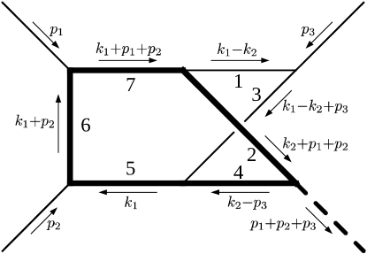
Refer to caption
Figure 1: The integral family with momenta and propagator labels.

As discussed in ref. Bonciani:2019jyb , six seven-propagator integral families contribute to the two-loop QCD contribution to H+jet𝐻𝑗𝑒𝑡H+jet production. Of these families, four are planar and have been computed in ref. Bonciani:2016qxi , and of the non-planar, one was computed in ref. Bonciani:2019jyb and the remaining one, denoted family G𝐺G, will be the topic of the present paper.

That integral family is defined by

Ia1a2a3a4a5a6a7a8a9subscriptIsubscript𝑎1subscript𝑎2subscript𝑎3subscript𝑎4subscript𝑎5subscript𝑎6subscript𝑎7subscript𝑎8subscript𝑎9\displaystyle\text{I}_{a_{1}a_{2}a_{3}a_{4}a_{5}a_{6}a_{7}a_{8}a_{9}} =e2γEϵdDk1dDk2(iπd/2)2P8a8P9a9P1a1P2a2P3a3P4a4P5a5P6a6P7a7absentsuperscript𝑒2subscript𝛾𝐸italic-ϵsuperscript𝑑𝐷subscript𝑘1superscript𝑑𝐷subscript𝑘2superscript𝑖superscript𝜋𝑑22superscriptsubscript𝑃8subscript𝑎8superscriptsubscript𝑃9subscript𝑎9superscriptsubscript𝑃1subscript𝑎1superscriptsubscript𝑃2subscript𝑎2superscriptsubscript𝑃3subscript𝑎3superscriptsubscript𝑃4subscript𝑎4superscriptsubscript𝑃5subscript𝑎5superscriptsubscript𝑃6subscript𝑎6superscriptsubscript𝑃7subscript𝑎7\displaystyle=e^{2\gamma_{E}\epsilon}\int\!\!\int\frac{d^{D}k_{1}d^{D}k_{2}}{(i\pi^{d/2})^{2}}\frac{P_{8}^{-a_{8}}\,P_{9}^{-a_{9}}}{P_{1}^{a_{1}}P_{2}^{a_{2}}P_{3}^{a_{3}}P_{4}^{a_{4}}P_{5}^{a_{5}}P_{6}^{a_{6}}P_{7}^{a_{7}}} (1)

where γE=Γ(1)subscript𝛾𝐸superscriptΓ1\gamma_{E}=-\Gamma^{\prime}(1) is the Euler-Mascheroni constant, and where

P1subscript𝑃1\displaystyle P_{1} =(k1k2)2,absentsuperscriptsubscript𝑘1subscript𝑘22\displaystyle=-(k_{1}-k_{2})^{2}, P4subscript𝑃4\displaystyle P_{4} =m2(k2p3)2,absentsuperscript𝑚2superscriptsubscript𝑘2subscript𝑝32\displaystyle=m^{2}-(k_{2}{-}p_{3})^{2}, P7subscript𝑃7\displaystyle P_{7} =m2(k1+p1+p2)2,absentsuperscript𝑚2superscriptsubscript𝑘1subscript𝑝1subscript𝑝22\displaystyle=m^{2}-(k_{1}{+}p_{1}{+}p_{2})^{2},
P2subscript𝑃2\displaystyle P_{2} =m2(k2+p1+p2)2,absentsuperscript𝑚2superscriptsubscript𝑘2subscript𝑝1subscript𝑝22\displaystyle=m^{2}-(k_{2}{+}p_{1}{+}p_{2})^{2}, P5subscript𝑃5\displaystyle P_{5} =m2k12,absentsuperscript𝑚2superscriptsubscript𝑘12\displaystyle=m^{2}-k_{1}^{2}, P8subscript𝑃8\displaystyle P_{8} =m2k22,absentsuperscript𝑚2superscriptsubscript𝑘22\displaystyle=m^{2}-k_{2}^{2}, (2)
P3subscript𝑃3\displaystyle P_{3} =(k1k2+p3)2,absentsuperscriptsubscript𝑘1subscript𝑘2subscript𝑝32\displaystyle=-(k_{1}{-}k_{2}{+}p_{3})^{2}, P6subscript𝑃6\displaystyle P_{6} =m2(k1+p2)2,absentsuperscript𝑚2superscriptsubscript𝑘1subscript𝑝22\displaystyle=m^{2}-(k_{1}{+}p_{2})^{2}, P9subscript𝑃9\displaystyle P_{9} =(k1k2p1)2.absentsuperscriptsubscript𝑘1subscript𝑘2subscript𝑝12\displaystyle=-(k_{1}{-}k_{2}{-}p_{1})^{2}.

Only P1subscript𝑃1P_{1}-P7subscript𝑃7P_{7} can appear as genuine propagators, so we have a8subscript𝑎8a_{8} and a9subscript𝑎9a_{9} restricted to the non-positive integers. The kinematics is p12=p22=p32=0superscriptsubscript𝑝12superscriptsubscript𝑝22superscriptsubscript𝑝320p_{1}^{2}=p_{2}^{2}=p_{3}^{2}=0 and additionally

s𝑠\displaystyle s (p1+p2)2,absentsuperscriptsubscript𝑝1subscript𝑝22\displaystyle\equiv(p_{1}{+}p_{2})^{2}, t𝑡\displaystyle t (p1+p3)2,absentsuperscriptsubscript𝑝1subscript𝑝32\displaystyle\equiv(p_{1}{+}p_{3})^{2}, u𝑢\displaystyle u (p2+p3)2,absentsuperscriptsubscript𝑝2subscript𝑝32\displaystyle\equiv(p_{2}{+}p_{3})^{2}, p42superscriptsubscript𝑝42\displaystyle p_{4}^{2} =(p1+p2+p3)2=s+t+u,absentsuperscriptsubscript𝑝1subscript𝑝2subscript𝑝32𝑠𝑡𝑢\displaystyle=(p_{1}{+}p_{2}{+}p_{3})^{2}=s{+}t{+}u, (3)

where m2superscript𝑚2m^{2} denotes the squared mass of the quark that couples to the Higgs, and p42superscriptsubscript𝑝42p_{4}^{2} the squared mass of the Higgs.

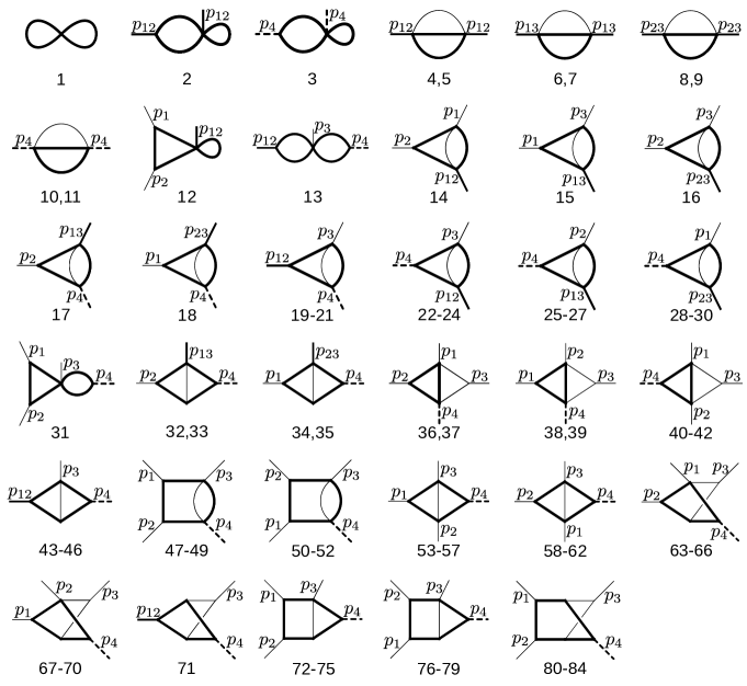
By using integration-by-parts (IBP) Tkachov:1981wb ; Chetyrkin:1981qh ; Laporta:1996mq ; Laporta:2001dd reduction methods Maierhoefer:2017hyi ; Smirnov:2019qkx , we identify a set of 84 master integrals for this family, whose diagrams are shown in Fig. 2. With those master integrals we defined a basis of Feynman integrals which is presented in Appendix A.
Refer to caption
Figure 2: The 84 master integrals. Shown on the figure is the sector, i.e. the set of propagators, to which the master integrals belong. Higher powers of propagators, numerators, or prefactors are not shown. External momenta are labelled using pij=pi+pjsubscript𝑝𝑖𝑗subscript𝑝𝑖subscript𝑝𝑗p_{ij}=p_{i}{+}p_{j} and p4=p1+p2+p3subscript𝑝4subscript𝑝1subscript𝑝2subscript𝑝3p_{4}=p_{1}{+}p_{2}{+}p_{3}. Masses (internal as well as external) are indicated with a thicker line.

3 Differential equations for the integral family

Given a basis of N𝑁N master integrals I(ϵ,s)𝐼italic-ϵ𝑠\vec{I}(\epsilon,\vec{s}), where ϵitalic-ϵ\epsilon is the dimensional regulator defined by D=42ϵ𝐷42italic-ϵD=4-2\epsilon and s={s1,,sn}𝑠subscript𝑠1subscript𝑠𝑛\vec{s}=\{s_{1},\ldots,s_{n}\} is a set of n𝑛n Lorentz invariants, it is possible to define a closed system of linear, first order differential equations Kotikov:1990kg ; Kotikov:1991pm ; Bern:1993kr ; Remiddi:1997ny ; Gehrmann:1999as for I(ϵ,si)𝐼italic-ϵsubscript𝑠𝑖\vec{I}(\epsilon,s_{i}) that in full generality reads,

siI(ϵ,s)=𝐌si(ϵ,s)I(ϵ,s),subscriptsubscript𝑠𝑖𝐼italic-ϵ𝑠subscript𝐌subscript𝑠𝑖italic-ϵ𝑠𝐼italic-ϵ𝑠\partial_{s_{i}}\vec{I}(\epsilon,\vec{s})=\mathbf{M}_{s_{i}}(\epsilon,\vec{s})\vec{I}(\epsilon,\vec{s}), (4)

where sisisubscriptsubscript𝑠𝑖subscript𝑠𝑖\partial_{s_{i}}\equiv\frac{\partial}{\partial s_{i}} and 𝐌sisubscript𝐌subscript𝑠𝑖\mathbf{M}_{s_{i}} is a set of N×N𝑁𝑁N\times N matrices.

The choice of the basis integrals is not unique, and by performing a basis change B=𝐓I𝐵𝐓𝐼\vec{B}=\mathbf{T}\vec{I} the differential equations transform according to,

siB(ϵ,s)=(𝐓𝐌si𝐓1(ϵ,s)𝐓si𝐓1(ϵ,s))B(ϵ,s).subscriptsubscript𝑠𝑖𝐵italic-ϵ𝑠subscript𝐓𝐌subscript𝑠𝑖superscript𝐓1italic-ϵ𝑠𝐓subscriptsubscript𝑠𝑖superscript𝐓1italic-ϵ𝑠𝐵italic-ϵ𝑠\partial_{s_{i}}\vec{B}(\epsilon,\vec{s})=\left(\mathbf{T}\mathbf{M}_{s_{i}}\mathbf{T}^{-1}(\epsilon,\vec{s})-\mathbf{T}\partial_{s_{i}}\mathbf{T}^{-1}(\epsilon,\vec{s})\right)\vec{B}(\epsilon,\vec{s})\,. (5)

In Ref. Henn:2013pwa it was conjectured that with a proper basis choice it is possible to cast the differential equations for Feynman integrals in the following simplified form,

siB(ϵ,s)=ϵ𝐀si(s)B(ϵ,s),subscriptsubscript𝑠𝑖𝐵italic-ϵ𝑠italic-ϵsubscript𝐀subscript𝑠𝑖𝑠𝐵italic-ϵ𝑠\partial_{s_{i}}\vec{B}(\epsilon,\vec{s})=\epsilon\mathbf{A}_{s_{i}}(\vec{s})\vec{B}(\epsilon,\vec{s})\,, (6)

where the dependence on ϵitalic-ϵ\epsilon is factorised out, and the matrices 𝐀si(s)subscript𝐀subscript𝑠𝑖𝑠\mathbf{A}_{s_{i}}(\vec{s}) depend only on the invariants s𝑠\vec{s}. Such a system of differential equations is said to be in canonical form, and the basis B𝐵\vec{B} is referred to as the canonical basis. A canonical system of differential equations is equivalent to the following equation in differential form,

dB(ϵ,s)=ϵd𝐀~(s)B(ϵ,s),𝑑𝐵italic-ϵ𝑠italic-ϵ𝑑~𝐀𝑠𝐵italic-ϵ𝑠d\vec{B}(\epsilon,\vec{s})=\epsilon\,d\tilde{\mathbf{A}}(\vec{s})\vec{B}(\epsilon,\vec{s})\,, (7)

where, by construction, the matrix 𝐀~~𝐀\tilde{\mathbf{A}} satisfies

si𝐀~(ϵ,s)=𝐀si(ϵ,s).subscriptsubscript𝑠𝑖~𝐀italic-ϵ𝑠subscript𝐀subscript𝑠𝑖italic-ϵ𝑠\partial_{s_{i}}\tilde{\mathbf{A}}(\epsilon,\vec{s})=\mathbf{A}_{s_{i}}(\epsilon,\vec{s})\,. (8)

The differential equation (7) can be formally solved in terms of a path-ordered exponential

B(ϵ,s)=𝒫exp(ϵγ𝑑𝐀~(s))B(ϵ,s0),𝐵italic-ϵ𝑠𝒫italic-ϵsubscript𝛾differential-d~𝐀𝑠𝐵italic-ϵsubscript𝑠0\vec{B}(\epsilon,\vec{s})=\mathcal{P}\exp\left(\epsilon\int_{\gamma}d\tilde{\mathbf{A}}(\vec{s})\right)\vec{B}(\epsilon,\vec{s}_{0})\,, (9)

where γ𝛾\gamma is an integration path connecting a boundary point s0subscript𝑠0\vec{s}_{0} to s𝑠\vec{s}, and 𝒫𝒫\mathcal{P} is the path-ordering operator. In dimensional regularization we are generally interested in a solution around ϵ=0italic-ϵ0\epsilon=0. By performing the expansion for small ϵitalic-ϵ\epsilon, the path-ordered exponential translates to iterated integrals over the entries of 𝐀~(s)~𝐀𝑠\tilde{\mathbf{A}}(\vec{s}). Specifically, the solution to all orders of ϵitalic-ϵ\epsilon is

B(ϵ,s)=B(ϵ,s0)+k1ϵkj=1k0tjt11γ(d𝐀~(t1))γ(d𝐀~(tj))B(kj)(s0),𝐵italic-ϵ𝑠𝐵italic-ϵsubscript𝑠0subscript𝑘1superscriptitalic-ϵ𝑘superscriptsubscript𝑗1𝑘subscript0subscript𝑡𝑗subscript𝑡11superscript𝛾𝑑~𝐀subscript𝑡1superscript𝛾𝑑~𝐀subscript𝑡𝑗superscript𝐵𝑘𝑗subscript𝑠0\vec{B}(\epsilon,\vec{s})=\vec{B}(\epsilon,\vec{s}_{0})+\sum_{k\geq 1}\epsilon^{k}\sum_{j=1}^{k}\int_{0\leq t_{j}\leq\ldots\leq t_{1}\leq 1}\gamma^{*}(d\tilde{\mathbf{A}}(t_{1}))\ldots\gamma^{*}(d\tilde{\mathbf{A}}(t_{j}))\,\vec{B}^{(k-j)}(\vec{s}_{0})\,, (10)

where γ:[0,1]n:𝛾01superscript𝑛\gamma:[0,1]\rightarrow\mathbb{R}^{n} and γ(d𝐀~(ti))=𝐀~(ti)tidtisuperscript𝛾𝑑~𝐀subscript𝑡𝑖~𝐀subscript𝑡𝑖subscript𝑡𝑖𝑑subscript𝑡𝑖\gamma^{*}(d\tilde{\mathbf{A}}(t_{i}))=\frac{\partial\tilde{\mathbf{A}}(t_{i})}{\partial t_{i}}dt_{i}, while B(i)(s)superscript𝐵𝑖𝑠\vec{B}^{(i)}(\vec{s}) denotes the i𝑖i-th coefficient of the ϵitalic-ϵ\epsilon-expansion.

So far we made no assumptions on the class of functions arising from the iterated integrals of Eq. (10). A large class of master integrals admits a canonical basis such that the matrix 𝐀~(s)~𝐀𝑠\tilde{\mathbf{A}}(\vec{s}) is a \mathbb{Q}-linear combination of logarithms of rational or algebraic arguments. This form also implies that the transformation 𝐓(ϵ,s)𝐓italic-ϵ𝑠\mathbf{T}(\epsilon,\vec{s}) to the canonical basis is rational or algebraic. The logarithms can be chosen in such a way that there are no \mathbb{Q}-linear relations between them. In the literature, the arguments of the independent logarithms are typically referred to as letters, while the set of letters is referred to as the alphabet.

If the alphabet contains only rational functions, the solutions can be directly expressed in terms of multiple polylogarithms Goncharov:1998kja , which are defined recursively as,

G(a1,a2,,an,x)=0xdtta1G(a2,,an,t),𝐺subscript𝑎1subscript𝑎2subscript𝑎𝑛𝑥superscriptsubscript0𝑥𝑑𝑡𝑡subscript𝑎1𝐺subscript𝑎2subscript𝑎𝑛𝑡G(a_{1},a_{2},\ldots,a_{n},x)=\int_{0}^{x}\frac{dt}{t-a_{1}}G(a_{2},\ldots,a_{n},t), (11)

with G(,x)1G(,x)\equiv 1 and G(0n,x)log(x)nn!G(\vec{0}_{n},x)\equiv\frac{\log(x)^{n}}{n!}. On the other hand, the general case where the alphabet contains algebraic functions is much less understood. In some cases it is possible to rationalize the algebraic functions by a suitable reparametrization of the invariants, reducing in this way the problem to a rational one. If a rational parametrization is not available, it is possible, in some case, to define an ansatz for the solution in terms of polylogarithms of suitably chosen (algebraic) arguments. The unknown parameters of the ansatz are then fixed by solving the differential equations and by imposing boundary conditions (see e.g. Brown:2009qja ; Goncharov.A.B.:2009tja ; Goncharov:2010jf ; Duhr:2011zq ; Bonciani:2016qxi ; Heller:2019gkq ; Bonciani:2019jyb ). Nonetheless, in the general algebraic case, it is not known whether the differential equations always admit a solution in terms of multiple polylogarithms.

More recently, a lot of progress has been made in the study of Feynman integrals which evaluate to elliptic generalizations of multiple polylogarithms (eMPLs) BrownLevin ; Broedel:2014vla ; Broedel:2017kkb ; Laporta:2004rb ; Kniehl:2005bc ; Adams:2013kgc ; Bloch:2013tra ; Bloch:2014qca ; Adams:2014vja ; Adams:2015gva ; Adams:2015ydq ; Remiddi:2016gno ; Primo:2016ebd ; Bonciani:2016qxi ; Adams:2016xah ; Passarino:2016zcd ; Harley:2017qut ; vonManteuffel:2017hms ; Ablinger:2017bjx ; Chen:2017pyi ; Hidding:2017jkk ; Bogner:2017vim ; Bourjaily:2017bsb ; Broedel:2017siw ; Laporta:2017okg ; Broedel:2018iwv ; Mistlberger:2018etf ; Lee:2018jsw ; Broedel:2018qkq ; Adams:2018bsn ; Adams:2018kez ; Broedel:2019hyg ; Bogner:2019lfa ; Kniehl:2019vwr ; Broedel:2019kmn . However, while in some cases it is possible to define a basis that casts the differential equations in canonical form (see e.g. Adams:2018yfj ; Adams:2018bsn ; Adams:2018kez ; Broedel:2019kmn ), little is known about their general analytic properties and how to systematically solve them in terms of elliptic multiple polylogarithms.

As we will see in the next sections, the differential equations for the integral family considered in this paper depend on complicated algebraic functions. Moreover some equations are coupled, and their solution involves functions of elliptic type. In this case finding a closed form solution for the integrals seems to be out of reach with current technology. Nonetheless, having phenomenological applications in mind, we follow a different approach, based on the series solution of the differential equations along contours in the space of the kinematic variables Francesco:2019yqt .

3.1 Canonical integrals

We denote the set of Lorentz invariants as s={s1,s2,s3,s4}={s,t,p42,m2}𝑠subscript𝑠1subscript𝑠2subscript𝑠3subscript𝑠4𝑠𝑡superscriptsubscript𝑝42superscript𝑚2\vec{s}=\{s_{1},s_{2},s_{3},s_{4}\}=\{s,t,p_{4}^{2},m^{2}\}. The first 71 master integrals of the basis chosen for family G are such that the system of differential equations are in canonical form. Namely, they satisfy Eq. (7). The matrix 𝐀~~𝐀\tilde{\mathbf{A}} can be constructed by using the following iterative definitions,

𝐀~1𝐀s1𝑑s1,𝐀~i(𝐀sisij=1i1𝐀j)𝑑si,i=2,,4,formulae-sequencesubscript~𝐀1subscript𝐀subscript𝑠1differential-dsubscript𝑠1formulae-sequencesubscript~𝐀𝑖subscript𝐀subscript𝑠𝑖subscriptsubscript𝑠𝑖superscriptsubscript𝑗1𝑖1subscript𝐀𝑗differential-dsubscript𝑠𝑖𝑖24\tilde{\mathbf{A}}_{1}\equiv\int\mathbf{A}_{s_{1}}ds_{1}\,,\quad\tilde{\mathbf{A}}_{i}\equiv\int\bigg{(}\mathbf{A}_{s_{i}}-\partial_{s_{i}}\sum_{j=1}^{i-1}\mathbf{A}_{j}\bigg{)}ds_{i}\,,~{}~{}~{}~{}i=2,...,4\,, (12)

and taking

𝐀~(ϵ,s)=i=14𝐀~i(ϵ,s).~𝐀italic-ϵ𝑠superscriptsubscript𝑖14subscript~𝐀𝑖italic-ϵ𝑠\tilde{\mathbf{A}}(\epsilon,\vec{s})=\sum_{i=1}^{4}\tilde{\mathbf{A}}_{i}(\epsilon,\vec{s}). (13)

For this integral family, the matrix 𝐀~(s)~𝐀𝑠\tilde{\mathbf{A}}(\vec{s}) is a \mathbb{Q}-linear combination of 76 logarithms depending on 11 different square roots. The full set of letters and square roots is presented in Appendix B. Because the letters contain numerous non-simultaneously rationalizable square roots, it is not manifest that the basis integrals admit polylogarithmic solutions at all orders in ϵitalic-ϵ\epsilon. We will nonetheless refer to the integral sectors composed of the first 71 integrals as the polylogarithmic sectors. This is motivated by the fact that it was shown in Refs. Bonciani:2016qxi ; Bonciani:2019jyb that the planar Higgs + jet integral families, and the non-planar integral family F, have similar canonical subsectors, for which polylogarithmic results were explicitly obtained at weight 2.

It will also be interesting to study the problem of finding polylogarithmic solutions for these sectors by using the methods recently put forward in Heller:2019gkq .

3.2 Elliptic integrals

In the following we will use the notation BiBjsubscript𝐵𝑖subscript𝐵𝑗B_{i}{-}B_{j} to denote the range of integrals Bi,Bi+1subscript𝐵𝑖subscript𝐵𝑖1B_{i},B_{i+1}, ,Bjsubscript𝐵𝑗\ldots,B_{j}. Similarly, we will use the notation Bijsubscript𝐵𝑖𝑗\vec{B}_{i-j} to denote the vector (Bi,Bi+1,,Bj)subscript𝐵𝑖subscript𝐵𝑖1subscript𝐵𝑗(B_{i},B_{i+1},\ldots,B_{j}).

Integrals B72B84subscript𝐵72subscript𝐵84B_{72}{-}B_{84} introduce functions of elliptic type. The appearance of functions of elliptic type can be observed at the level of the maximal cut, which gives an indication of the type of functions which appear in the full solution for the integrals in a given sector. When the maximal cut of an integral is elliptic, we expect that the integral cannot be expressed Primo:2016ebd ; Frellesvig:2017aai ; Bosma:2017ens ; Harley:2017qut ; Primo:2017ipr in terms of multiple polylogarithms. Let us discuss the maximal cut for integrals B72B84subscript𝐵72subscript𝐵84B_{72}{-}B_{84}. These integrals define three integral sectors, i.e. B72B75subscript𝐵72subscript𝐵75B_{72}{-}B_{75}, B76B79subscript𝐵76subscript𝐵79B_{76}{-}B_{79} and B80B84subscript𝐵80subscript𝐵84B_{80}{-}B_{84}. Performing the maximal cuts of the basic integral in each of these sectors in d=4𝑑4d=4 we get, using the loop-by-loop Baikov representation Frellesvig:2017aai ; Harley:2017qut 111The maximal cut can also be computed by using the loop-by-loop approach in momentum space Primo:2016ebd ., the univariate integrals,

B72B75:Cut(I0111111100):subscript𝐵72subscript𝐵75CutsubscriptI0111111100\displaystyle B_{72}{-}B_{75}:\;\;\text{Cut}(\text{I}_{0111111100}) =dzs((z+p42)24m2p42)((z+t)2+4m2tu/s),absent𝑑𝑧𝑠superscript𝑧superscriptsubscript𝑝4224superscript𝑚2superscriptsubscript𝑝42superscript𝑧𝑡24superscript𝑚2𝑡𝑢𝑠\displaystyle=\int\frac{dz}{s\sqrt{\big{(}(z{+}p_{4}^{2})^{2}{-}4m^{2}p_{4}^{2}\big{)}\,\big{(}(z{+}t)^{2}{+}4m^{2}tu/s\big{)}}}, (14)
B76B79:Cut(I1101111100):subscript𝐵76subscript𝐵79CutsubscriptI1101111100\displaystyle B_{76}{-}B_{79}:\;\;\text{Cut}(\text{I}_{1101111100}) =dzs((z+p42)24m2p42)((z+u)2+4m2tu/s),absent𝑑𝑧𝑠superscript𝑧superscriptsubscript𝑝4224superscript𝑚2superscriptsubscript𝑝42superscript𝑧𝑢24superscript𝑚2𝑡𝑢𝑠\displaystyle=\int\frac{dz}{s\sqrt{\big{(}(z{+}p_{4}^{2})^{2}{-}4m^{2}p_{4}^{2}\big{)}\,\big{(}(z{+}u)^{2}{+}4m^{2}tu/s\big{)}}}, (15)
B80B84:Cut(I1111111100):subscript𝐵80subscript𝐵84CutsubscriptI1111111100\displaystyle B_{80}{-}B_{84}:\;\;\text{Cut}(\text{I}_{1111111100}) =dzsz(z+p42s)(z+t)2+4m2tu/s.absent𝑑𝑧𝑠𝑧𝑧superscriptsubscript𝑝42𝑠superscript𝑧𝑡24superscript𝑚2𝑡𝑢𝑠\displaystyle=\int\frac{dz}{s\,z\,(z{+}p_{4}^{2}{-}s)\,\sqrt{(z{+}t)^{2}{+}4m^{2}tu/s}}. (16)

The first two of these evaluate to elliptic integrals of the first kind, while the latter evaluates to a combination of logarithms. This corresponds to the two elliptic curves,

y2superscript𝑦2\displaystyle y^{2} =((z+p42)24m2p42)((z+t)2+4m2tu/s),absentsuperscript𝑧superscriptsubscript𝑝4224superscript𝑚2superscriptsubscript𝑝42superscript𝑧𝑡24superscript𝑚2𝑡𝑢𝑠\displaystyle=\big{(}(z{+}p_{4}^{2})^{2}{-}4m^{2}p_{4}^{2}\big{)}\,\big{(}(z{+}t)^{2}{+}4m^{2}tu/s\big{)},
y2superscript𝑦2\displaystyle y^{2} =((z+p42)24m2p42)((z+u)2+4m2tu/s),absentsuperscript𝑧superscriptsubscript𝑝4224superscript𝑚2superscriptsubscript𝑝42superscript𝑧𝑢24superscript𝑚2𝑡𝑢𝑠\displaystyle=\big{(}(z{+}p_{4}^{2})^{2}{-}4m^{2}p_{4}^{2}\big{)}\,\big{(}(z{+}u)^{2}{+}4m^{2}tu/s\big{)}, (17)

being present in the results.

The integrals B72B75subscript𝐵72subscript𝐵75B_{72}{-}B_{75} are planar, and indeed that sector is equivalent to the sector of the integral A66subscript𝐴66A_{66} discussed in refs Bonciani:2016qxi ; Francesco:2019yqt . Likewise the integrals B76B79subscript𝐵76subscript𝐵79B_{76}{-}B_{79} are merely a crossing thereof with p1p2subscript𝑝1subscript𝑝2p_{1}\leftrightarrow p_{2}, corresponding to tu𝑡𝑢t\leftrightarrow u. The fact that eq. (16) does not evaluate to elliptic integrals does not mean that such structures are absent in the un-cut integrals, as elliptic curves would appear at the sub-maximal cuts corresponding to the sectors B72B75subscript𝐵72subscript𝐵75B_{72}{-}B_{75} and B76B79subscript𝐵76subscript𝐵79B_{76}{-}B_{79}.

The appearance of functions of elliptic type can be also observed by analyzing the relevant system of differential equations. Integrals B72B84subscript𝐵72subscript𝐵84B_{72}{-}B_{84} satisfy,

siB7284(s,ϵ)=j=0ϵj𝐀si(j)(s)B7284(s,ϵ)+G7284(s,ϵ),subscript𝑠𝑖subscript𝐵7284𝑠italic-ϵsuperscriptsubscript𝑗0superscriptitalic-ϵ𝑗superscriptsubscriptsuperscript𝐀subscript𝑠𝑖𝑗𝑠subscript𝐵7284𝑠italic-ϵsubscript𝐺7284𝑠italic-ϵ\frac{\partial}{\partial s_{i}}\vec{B}_{72-84}(\vec{s},\epsilon)=\sum_{j=0}^{\infty}\epsilon^{j}\mathbf{A^{\prime}}_{s_{i}}^{(j)}(\vec{s})\vec{B}_{72-84}(\vec{s},\epsilon)+\vec{G}_{72-84}(\vec{s},\epsilon), (18)

where the vector G7284(s,ϵ)subscript𝐺7284𝑠italic-ϵ\vec{G}_{72-84}(\vec{s},\epsilon) depends on the canonical integrals B171(s,ϵ)subscript𝐵171𝑠italic-ϵ\vec{B}_{1-71}(\vec{s},\epsilon), and the homogeneous matrix has the schematic form,

𝐀si(0)(s)=( 0 0 0 0 0 0 0 0 0 0 0000000000000000000000000000000000000000000000000000000000000000000000000000000000000000000000000000000000000000000000000),superscriptsubscriptsuperscript𝐀subscript𝑠𝑖0𝑠 0 0 0 0 0 0 0 0 0 0 000000000000000000000000000000000missing-subexpressionmissing-subexpressionmissing-subexpressionmissing-subexpressionmissing-subexpressionmissing-subexpressionmissing-subexpressionmissing-subexpressionmissing-subexpressionmissing-subexpressionmissing-subexpressionmissing-subexpressionmissing-subexpression0000000000000000000000000000000000000000000missing-subexpressionmissing-subexpressionmissing-subexpressionmissing-subexpressionmissing-subexpressionmissing-subexpressionmissing-subexpressionmissing-subexpressionmissing-subexpressionmissing-subexpressionmissing-subexpressionmissing-subexpressionmissing-subexpression000000000000000000000000000000000000000000000\mathbf{A^{\prime}}_{s_{i}}^{(0)}(\vec{s})=\left(\begin{array}[]{cccc|cccc|ccccc}\bm{*}&\;0&\;0&\bm{*}&\;0&\;0&\;0&\;0&\;0&\;0&\;0&\;0&\;0\\ \bm{*}&0&0&\bm{*}&0&0&0&0&0&0&0&0&0\\ \bm{*}&0&\bm{*}&\bm{*}&0&0&0&0&0&0&0&0&0\\ \bm{*}&0&0&\bm{*}&0&0&0&0&0&0&0&0&0\\ \hline\cr 0&0&0&0&\bm{*}&0&0&\bm{*}&0&0&0&0&0\\ 0&0&0&0&\bm{*}&0&0&\bm{*}&0&0&0&0&0\\ 0&0&0&0&\bm{*}&0&\bm{*}&\bm{*}&0&0&0&0&0\\ 0&0&0&0&\bm{*}&0&0&\bm{*}&0&0&0&0&0\\ \hline\cr\bm{*}&0&0&\bm{*}&\bm{*}&0&0&\bm{*}&0&0&0&0&0\\ \bm{*}&0&0&\bm{*}&\bm{*}&0&0&\bm{*}&0&0&0&0&0\\ \bm{*}&0&0&\bm{*}&\bm{*}&0&0&\bm{*}&0&0&0&0&0\\ \bm{*}&0&0&\bm{*}&\bm{*}&0&0&\bm{*}&0&0&0&0&0\\ \bm{*}&0&0&\bm{*}&\bm{*}&0&0&\bm{*}&0&0&0&0&0\\ \end{array}\right), (19)

where the lines separate the 3 elliptic sectors. In Primo:2016ebd it was observed that the homogeneous differential equation of a given integral is solved by the maximally cut integral. This implies that, when the maximal cut is elliptic, the solution of the integral can be expressed in terms of iterated integrals over functions of elliptic type. As seen from Eqs. (14) and (15), we encounter this scenario for integrals B72B75subscript𝐵72subscript𝐵75B_{72}{-}B_{75} and B76B79subscript𝐵76subscript𝐵79B_{76}{-}B_{79}. On the other hand, the maximal cut of sector B80B84subscript𝐵80subscript𝐵84B_{80}{-}B_{84} is logarithmic. However, as seen from Eq. (19), this sector couples to the lower elliptic sectors via inhomogeneous terms of the differential equations, implying that these integrals can be expressed in terms of iterated integrals over the same functions of elliptic type.

We remark that the presence of multiple elliptic curves renders the functional form of the solution an open problem (but see e.g. Adams:2018bsn for progress in this direction).

4 Series expansion along contours

We consider the series expansion strategy outlined in Bonciani:2019jyb ; Francesco:2019yqt (see also Pozzorini:2005ff ; Aglietti:2007as ; Mueller:2015lrx ; Lee:2017qql ; Lee:2018ojn ; Bonciani:2018uvv ; Mistlberger:2018etf for the application of expansion methods to single scale processes, and  Melnikov:2016qoc ; Melnikov:2017pgf ; Bonciani:2018omm ; Bruser:2018jnc ; Davies:2018ood ; Davies:2018qvx for expansion methods applied to multiscale problems in particular kinematic limits). The strategy relies on parametrizing the integrals along straight line segments, for which we solve the corresponding differential equations in terms of one-dimensional generalized series. We briefly review the strategy here, and highlight aspects that are specific to the integral family under consideration. We start from the system of differential equations of the basis defined in Appendix A, which has the form,

dB=𝐌B,𝑑𝐵𝐌𝐵\displaystyle d\vec{B}=\mathbf{M}\vec{B}\,, (20)

where 𝐌=si𝐌si(ϵ,s)dsi𝐌subscriptsubscript𝑠𝑖subscript𝐌subscript𝑠𝑖italic-ϵ𝑠𝑑subscript𝑠𝑖\mathbf{M}=\sum_{s_{i}}\mathbf{M}_{s_{i}}(\epsilon,\vec{s})ds_{i}, and where we otherwise suppress variable dependence in the notation. For convenience, we put m2=1superscript𝑚21m^{2}=1 without loss of generality. We consider a generic line parametrized as,

γ(λ)={γs(λ),γt(λ),γp42(λ)}.𝛾𝜆subscript𝛾𝑠𝜆subscript𝛾𝑡𝜆subscript𝛾superscriptsubscript𝑝42𝜆\vec{\gamma}(\lambda)=\{\gamma_{s}(\lambda),\gamma_{t}(\lambda),\gamma_{p_{4}^{2}}(\lambda)\}\,. (21)

The differential equations along this line take the form,

λB=𝐌λB,𝜆𝐵subscript𝐌𝜆𝐵\displaystyle\frac{\partial}{\partial\lambda}\vec{B}=\mathbf{M}_{\lambda}\vec{B}\,, (22)

where 𝐌λ=si𝐌si(ϵ,s)γsiλsubscript𝐌𝜆subscriptsubscript𝑠𝑖subscript𝐌subscript𝑠𝑖italic-ϵ𝑠subscript𝛾subscript𝑠𝑖𝜆\mathbf{M}_{\lambda}=\sum_{s_{i}}\mathbf{M}_{s_{i}}(\epsilon,\vec{s})\frac{\partial\gamma_{s_{i}}}{\partial\lambda}. Next, we expand the differential equations in ϵitalic-ϵ\epsilon to obtain a system for each order in ϵitalic-ϵ\epsilon. In particular, we let,

B=k=0B(k)ϵk,𝐌=k=0𝐌(k)ϵk.formulae-sequence𝐵superscriptsubscript𝑘0superscript𝐵𝑘superscriptitalic-ϵ𝑘𝐌superscriptsubscript𝑘0superscript𝐌𝑘superscriptitalic-ϵ𝑘\displaystyle\vec{B}=\sum_{k=0}^{\infty}B^{(k)}\epsilon^{k},\quad\mathbf{M}=\sum_{k=0}^{\infty}\mathbf{M}^{(k)}\epsilon^{k}\,. (23)

Note that both expansions start at finite order for our choice of basis. The system of differential equations now takes the following form, order-by-order in ϵitalic-ϵ\epsilon,

λB(i)=𝐌λ(0)B(i)+k=1i𝐌λ(k)B(ik),𝜆superscript𝐵𝑖subscriptsuperscript𝐌0𝜆superscript𝐵𝑖superscriptsubscript𝑘1𝑖superscriptsubscript𝐌𝜆𝑘superscript𝐵𝑖𝑘\displaystyle\frac{\partial}{\partial\lambda}\vec{B}^{(i)}=\mathbf{M}^{(0)}_{\lambda}\vec{B}^{(i)}+\sum_{k=1}^{i}\mathbf{M}_{\lambda}^{(k)}\vec{B}^{(i-k)}\,, (24)

where we separated out the homogeneous part 𝐌λ(0)B(i)subscriptsuperscript𝐌0𝜆superscript𝐵𝑖\mathbf{M}^{(0)}_{\lambda}\vec{B}^{(i)} from the inhomogeneous part. The homogeneous matrix 𝐌(0)superscript𝐌0\mathbf{M}^{(0)} determines the sequence in which the individual integrals should be integrated, and which integrals are coupled.

Let us consider first the polylogarithmic sectors and review the series solution strategy for those. The system of differential equations becomes simply,

λB(i)=𝐌λ(1)B(i1),𝜆superscript𝐵𝑖superscriptsubscript𝐌𝜆1superscript𝐵𝑖1\displaystyle\frac{\partial}{\partial\lambda}\vec{B}^{(i)}=\mathbf{M}_{\lambda}^{(1)}\vec{B}^{(i-1)}\,, (25)

where 𝐌λ(1)superscriptsubscript𝐌𝜆1\mathbf{M}_{\lambda}^{(1)} = ϵ(𝐀~/λ)italic-ϵ~𝐀𝜆\epsilon\left(\partial\tilde{\mathbf{A}}/\partial\lambda\right), and 𝐀~~𝐀\tilde{\mathbf{A}} was defined in Eq. (7). Hence, the work for the polylogarithmic sectors amounts to solving a sequence of first order differential equations without homogeneous parts. The general solution is easily found from a single integration,

B(i)(λ)=λ0λ1𝐌λ(1)B(i1)𝑑λ+B(i)(λ0).superscript𝐵𝑖𝜆superscriptsubscriptsubscript𝜆0subscript𝜆1superscriptsubscript𝐌𝜆1superscript𝐵𝑖1differential-d𝜆superscript𝐵𝑖subscript𝜆0\displaystyle\vec{B}^{(i)}(\lambda)=\int_{\lambda_{0}}^{\lambda_{1}}\mathbf{M}_{\lambda}^{(1)}\vec{B}^{(i-1)}d\lambda+\vec{B}^{(i)}(\lambda_{0})\,. (26)

Importantly, we solve the integration by performing series expansions in λ𝜆\lambda. The only algebraic terms in our basis and in the matrices are square roots, so that the expansions of the matrix elements are in terms of integer and half-integer powers of λ𝜆\lambda. After integrating, the series expansions will also contain logarithmic terms. Therefore, in general each integration in Eq. (26) is of the form,

λqlog(λ)p,\displaystyle\int\lambda^{q}\log(\lambda)^{p}\,, (27)

where q𝑞q is an integer or half-integer, and p𝑝p is a non-negative integer. It may easily be verified that such integrals evaluate to sums of terms of the same type, by using integration-by-parts identities to reduce the power of the logarithm inside the integral.

As shown in Eq. (19), we simplified our basis in such a way that in each elliptic sector at most 2 integrals are coupled together, specifically the pairs of integrals B72subscript𝐵72B_{72}, B75subscript𝐵75B_{75} and B76subscript𝐵76B_{76}, B79subscript𝐵79B_{79}. These integrals can be solved by combining their first order differential equations into second order differential equations. Integrals B74subscript𝐵74B_{74} and B78subscript𝐵78B_{78} can be solved from their first order differential equation, but, in contrast to the polylogarithmic sectors, their differential equations have a homogeneous component. Lastly, integrals B73subscript𝐵73B_{73}, B77subscript𝐵77B_{77}, B80subscript𝐵80B_{80}, B81subscript𝐵81B_{81}, and B82subscript𝐵82B_{82} satisfy a first order differential equation without a homogeneous component, and can be solved in the same manner as the polylogarithmic integrals. For completeness, we discuss solving these two cases next.

Consider a first order differential equation with homogeneous component of the form,

f(λ)+a(λ)f(λ)+b(λ)=0.superscript𝑓𝜆𝑎𝜆𝑓𝜆𝑏𝜆0\displaystyle f^{\prime}(\lambda)+a(\lambda)f(\lambda)+b(\lambda)=0\,. (28)

The solution to the homogeneous part is easily found to be,

μ(λ)=ea(λ)𝑑λ,𝜇𝜆superscript𝑒𝑎𝜆differential-d𝜆\displaystyle\mu(\lambda)=e^{-\int a(\lambda)d\lambda}\,, (29)

up to an arbitrary multiplicative constant. The full solution to Eq. (28) is then given in terms of μ(λ)𝜇𝜆\mu(\lambda) by,

f(λ)=μ(λ)[b(λ)μ(λ)𝑑λ+c].𝑓𝜆𝜇𝜆delimited-[]𝑏𝜆𝜇𝜆differential-d𝜆𝑐\displaystyle f(\lambda)=\mu(\lambda)\left[-\int\frac{b(\lambda)}{\mu(\lambda)}d\lambda+c\right]\,. (30)

Now, consider a second order differential equation of the form,

f′′(λ)+a(λ)f(λ)+b(λ)f(λ)+c(λ)=0.superscript𝑓′′𝜆𝑎𝜆superscript𝑓𝜆𝑏𝜆𝑓𝜆𝑐𝜆0\displaystyle f^{\prime\prime}(\lambda)+a(\lambda)f^{\prime}(\lambda)+b(\lambda)f(\lambda)+c(\lambda)=0\,. (31)

Given two solutions μ1(λ)subscript𝜇1𝜆\mu_{1}(\lambda) and μ2(λ)subscript𝜇2𝜆\mu_{2}(\lambda) to the homogeneous part of the differential equation, the general solution can be written using the method of variation of parameters as

f(λ)𝑓𝜆\displaystyle f(\lambda) =μ1(λ)μ2(λ)c(λ)μ1(λ)μ2(λ)μ2(λ)μ1(λ)𝑑λμ2(λ)μ1(λ)c(λ)μ1(λ)μ2(λ)μ2(λ)μ1(λ)𝑑λabsentsubscript𝜇1𝜆subscript𝜇2𝜆𝑐𝜆subscript𝜇1𝜆superscriptsubscript𝜇2𝜆subscript𝜇2𝜆superscriptsubscript𝜇1𝜆differential-d𝜆subscript𝜇2𝜆subscript𝜇1𝜆𝑐𝜆subscript𝜇1𝜆superscriptsubscript𝜇2𝜆subscript𝜇2𝜆superscriptsubscript𝜇1𝜆differential-d𝜆\displaystyle=\mu_{1}(\lambda)\int\frac{\mu_{2}(\lambda)c(\lambda)}{\mu_{1}(\lambda)\mu_{2}^{\prime}(\lambda)-\mu_{2}(\lambda)\mu_{1}^{\prime}(\lambda)}d\lambda\ -\mu_{2}(\lambda)\int\frac{\mu_{1}(\lambda)c(\lambda)}{\mu_{1}(\lambda)\mu_{2}^{\prime}(\lambda)-\mu_{2}(\lambda)\mu_{1}^{\prime}(\lambda)}d\lambda
+d1μ1(λ)+d2μ2(λ),subscript𝑑1subscript𝜇1𝜆subscript𝑑2subscript𝜇2𝜆\displaystyle+d_{1}\mu_{1}(\lambda)+d_{2}\mu_{2}(\lambda)\,, (32)

where d1subscript𝑑1d_{1} and d2subscript𝑑2d_{2} are complex constants to be fixed from boundary conditions. The remaining challenge is to find two distinct homogeneous solutions μ1(λ)subscript𝜇1𝜆\mu_{1}(\lambda) and μ2(λ)subscript𝜇2𝜆\mu_{2}(\lambda) that are not related by a rescaling. From the well-known Frobenius method (see e.g. Coddington for an extensive review of the method), it follows that we may always find one series solution of the form μ1(λ)=λr+λrk=1μ1,kλksubscript𝜇1𝜆superscript𝜆𝑟superscript𝜆𝑟superscriptsubscript𝑘1subscript𝜇1𝑘superscript𝜆𝑘\mu_{1}(\lambda)=\lambda^{r}+\lambda^{r}\sum_{k=1}^{\infty}\mu_{1,k}\lambda^{k}. The values for r𝑟r and μ1,ksubscript𝜇1𝑘\mu_{1,k} may be found up to the desired order in λ𝜆\lambda by plugging μ1(λ)subscript𝜇1𝜆\mu_{1}(\lambda) into the homogeneous differential equation as an ansatz, and solving order-by-order in λ𝜆\lambda for the unknowns. The lowest order in λ𝜆\lambda gives a quadratic equation in r𝑟r called the indicial equation. By picking r𝑟r to be the largest root of the indicial equation, it is guaranteed that we may solve for the remaining unknowns μ1,ksubscript𝜇1𝑘\mu_{1,k} with k1𝑘1k\geq 1.

It remains to find a second homogeneous solution. This may be done in the following way. First we write the second homogeneous solution μ2(λ)subscript𝜇2𝜆\mu_{2}(\lambda) as μ2(λ)=μ1(λ)h(λ)subscript𝜇2𝜆subscript𝜇1𝜆𝜆\mu_{2}(\lambda)=\mu_{1}(\lambda)h(\lambda). Plugging this expression into the homogeneous part of Eq. (31), we find a new equation,

μ1(λ)h′′(λ)+h(λ)(a(λ)μ1(λ)+2μ1(λ))=0,subscript𝜇1𝜆superscript′′𝜆superscript𝜆𝑎𝜆subscript𝜇1𝜆2superscriptsubscript𝜇1𝜆0\displaystyle\mu_{1}(\lambda)h^{\prime\prime}(\lambda)+h^{\prime}(\lambda)\left(a(\lambda)\mu_{1}(\lambda)+2\mu_{1}^{\prime}(\lambda)\right)=0\,, (33)

which we recognize as a first order homogeneous differential equation for h(λ)superscript𝜆h^{\prime}(\lambda), which we know how to solve. This way, we obtain the second homogeneous solution μ2(λ)subscript𝜇2𝜆\mu_{2}(\lambda). Thus we may now use Eq. (4) to compute the full solution to Eq. (31).

4.1 Boundary conditions

To fix our system of differential equations we need a suitable boundary point. Similar to Bonciani:2019jyb , we work in the heavy mass limit parametrized by,

γhm(λ)={sλ,tλ,p42λ},subscript𝛾𝑚𝜆𝑠𝜆𝑡𝜆superscriptsubscript𝑝42𝜆\displaystyle\gamma_{hm}(\lambda)=\{s\lambda,t\lambda,p_{4}^{2}\lambda\}\,, (34)

where λ𝜆\lambda is a line parameter that goes to zero. Using the method of asymptotic expansions in the parametric representation Beneke:1997zp ; Jantzen:2011nz ; Semenova:2018cwy ; Smirnov:1999bza ; Pak:2010pt ; Jantzen:2012mw , we may obtain values of our basis integrals in the heavy mass limit. The final result turns out to be very simple,

limλ0B1(γhm(λ))=e2γEϵΓ(1+ϵ)2(m2)2ϵ,limλ0Bi(γhm(λ))=0 for i=2,,84.formulae-sequencesubscript𝜆0subscript𝐵1subscript𝛾𝑚𝜆superscript𝑒2subscript𝛾𝐸italic-ϵΓsuperscript1italic-ϵ2superscriptsuperscript𝑚22italic-ϵformulae-sequencesubscript𝜆0subscript𝐵𝑖subscript𝛾𝑚𝜆0 for 𝑖284\displaystyle\lim_{\lambda\rightarrow 0}B_{1}(\gamma_{hm}(\lambda))=e^{2\gamma_{E}\epsilon}\Gamma(1+\epsilon)^{2}(m^{2})^{-2\epsilon}\,,\quad\lim_{\lambda\rightarrow 0}B_{i}(\gamma_{hm}(\lambda))=0\quad\text{ for }i=2,\ldots,84\,. (35)

We note that the homogeneous solution of the differential equation for B78subscript𝐵78B_{78} along γhm(λ)subscript𝛾𝑚𝜆\gamma_{hm}(\lambda) is proportional to λ𝜆\lambda, and hence we are not able to determine the boundary constant for B78subscript𝐵78B_{78} directly from Eq. (35). It may be verified that B78subscript𝐵78B_{78} is also zero at order λ1superscript𝜆1\lambda^{1} in the heavy mass limit, and hence the constant multiplying the homogeneous solution may be put to zero for this integral.

4.2 Convergence of the series

A trait of the expansion strategy is that each expansion at a given point along a line has a limited range of convergence. Namely, each expansion at a given point is valid up to the distance of the point to the nearest singularity. Thus, to obtain results along a given line, numerous expansions along segments of the line have to be patched together in order to reach a given point in phase space. In particular, to cross a singularity we may perform an expansion at the singularity, and fix its boundary conditions from an expansion at a neighbouring point along the line. We employ the following strategy for deciding along which line segments to expand:

  • First we create a list A𝐴A of all singularities of the matrix elements of 𝐌λsubscript𝐌𝜆\mathbf{M}_{\lambda} on the line γ(λ)𝛾𝜆\gamma(\lambda) along which we seek to integrate. By singular point we mean any non-analytic point of the differential equations. In our case, these are the zeros of the denominators of the matrix elements, and the zeros of the square roots.

  • Some of the singularities may be complex. We replace each complex singularity λsing=λresing+iλimsingsuperscript𝜆singsubscriptsuperscript𝜆sing𝑟𝑒𝑖subscriptsuperscript𝜆sing𝑖𝑚\lambda^{\text{sing}}=\lambda^{\text{sing}}_{re}+i\lambda^{\text{sing}}_{im} in the list A𝐴A by three real points: λresingλimsingsubscriptsuperscript𝜆sing𝑟𝑒subscriptsuperscript𝜆sing𝑖𝑚\lambda^{\text{sing}}_{re}-\lambda^{\text{sing}}_{im}, λresingsubscriptsuperscript𝜆sing𝑟𝑒\lambda^{\text{sing}}_{re} and λresing+λimsingsubscriptsuperscript𝜆sing𝑟𝑒subscriptsuperscript𝜆sing𝑖𝑚\lambda^{\text{sing}}_{re}+\lambda^{\text{sing}}_{im} .

  • Next, we consider a Möbius transformation λ=g(λ)𝜆𝑔superscript𝜆\lambda=g(\lambda^{\prime}) for each triplet (a,b,c)𝑎𝑏𝑐(a,b,c) of neighbouring points in A𝐴A, such that g1({a,b,c})={1,0,1}superscript𝑔1𝑎𝑏𝑐101g^{-1}(\{a,b,c\})=\{-1,0,1\}. Note that a series (in λsuperscript𝜆\lambda^{\prime}) centered at λ=0superscript𝜆0\lambda^{\prime}=0 will have a radius of convergence greater than or equal to 1.

  • To obtain results along γ(λ)𝛾𝜆\gamma(\lambda) from λ0subscript𝜆0\lambda_{0} to λ1subscript𝜆1\lambda_{1}, we have to match expansions along neighbouring line segments, which are expressed in terms of Möbius transformed line parameters, say λsuperscript𝜆\lambda^{\prime} and λ′′superscript𝜆′′\lambda^{\prime\prime}. We may find a matching point between two neighbouring expansions by solving λ=λ′′superscript𝜆superscript𝜆′′\lambda^{\prime}=-\lambda^{\prime\prime}, assuming λ′′superscript𝜆′′\lambda^{\prime\prime} corresponds to the line segments lying on the right.

  • In general, one may find that this condition picks λsuperscript𝜆\lambda^{\prime} and λ′′superscript𝜆′′\lambda^{\prime\prime} to be very close to 1 and -1, respectively, where both series may be very slowly converging. This can be solved by adding additional expansion points along the line segments. In particular, we may consider new expansion points between -1 and 1, such that upon matching neighbouring expansions, neither gets evaluated further than a certain fraction of the distance to the nearest singularity. We will refer to the inverse of this fraction by the parameter k𝑘k. For example, with k𝑘k = 2, the expansion points are chosen such that no series is evaluated beyond half its radius of convergence. The situation is illustrated in Figure 3. By choosing higher values of k𝑘k, we will increase the precision of the results, since the expansions along each line segment are evaluated closer to the origin.

We note that in general we may encounter both spurious, physical, and non-physical singularities. The spurious singularities are singularities that only appear in the elements of 𝐌𝐌\mathbf{M}, but which are not singularities of the basis integrals themselves. The physical singularities are threshold singularities, in our case s=4m2𝑠4superscript𝑚2s=4m^{2} and p42=4m2superscriptsubscript𝑝424superscript𝑚2p_{4}^{2}=4m^{2}. For those, it is important to cross the singularity according to Feynman prescription, which tells us to interpret s𝑠s and p42superscriptsubscript𝑝42p_{4}^{2} as having an infinitesimally small positive imaginary part. Furthermore, we should make sure to assign the same imaginary part to the square roots in our basis that are associated with physical singularities. Specifically, some of our basis integrals have the prefactors 4m2p424superscript𝑚2superscriptsubscript𝑝42\sqrt{4m^{2}-p_{4}^{2}} and 4m2s4superscript𝑚2𝑠\sqrt{4m^{2}-s}, which are analytically continued as 4m2p42iδ4superscript𝑚2superscriptsubscript𝑝42𝑖𝛿\sqrt{4m^{2}-p_{4}^{2}-i\delta} and 4m2siδ4superscript𝑚2𝑠𝑖𝛿\sqrt{4m^{2}-s-i\delta} for an infinitesimally small δ>0𝛿0\delta>0. Lastly, there are also non-physical singularities, which can arise from rational prefactors in the basis, or from square roots in the basis that do not correspond to physical singularities. Since these singularities are introduced by the basis choice, we are free to assign every non-physical root in the basis the standard branch, i.e. we consider the argument to carry the imaginary part +iδ𝑖𝛿+i\delta.

Refer to caption
(a)
Refer to caption
(b)
Figure 3: These figures illustrate subdivisions of an expansion in the unit interval [-1,1] with singularities at 1,010-1,0 and 111, in terms of additional expansions, such that each expansion can be matched to the next one at a fixed fraction of the distance to its nearest singularities. The numbers on top are the matching points between neighbouring expansions, while the numbers at the bottom indicate the expansions points for (a) k=2𝑘2k=2: Moving at most half the distance to the nearest singularity, (b) k=3𝑘3k=3: Moving at most one-third the distance to the nearest singularity.

To improve the convergence of our series solutions, we compute their diagonal Padé approximants and evaluate those instead at each (matching) point. Since we are dealing with generalized series that may in general include powers of logarithms, we collect first on powers of logarithms and compute the Padé approximant for each series that multiplies a given power.
Refer to caption
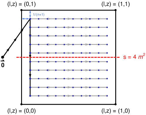
Figure 4: Depiction of lines along which we produce samples in the physical region of the top. The black lines 0(1/(n+1),n/(n+1))(1/(n+1),1/(n+1))01𝑛1𝑛𝑛11𝑛11𝑛1\vec{0}\rightarrow\left(1/(n+1),n/(n+1)\right)\rightarrow\left(1/(n+1),1/(n+1)\right) are computed first to obtain boundary values for n𝑛n horizontal lines, depicted in grey. The horizontal lines are themselves used to produce n𝑛n evenly spaced samples, denoted by blue dots. The particle production threshold s=4m2𝑠4superscript𝑚2s=4m^{2} is depicted by a dashed red line. Depicted is the case with n=10𝑛10n=10. The actual plots are produced with n=100𝑛100n=100.

5 Results for top and bottom quarks

Refer to caption Refer to caption Refer to caption Refer to caption
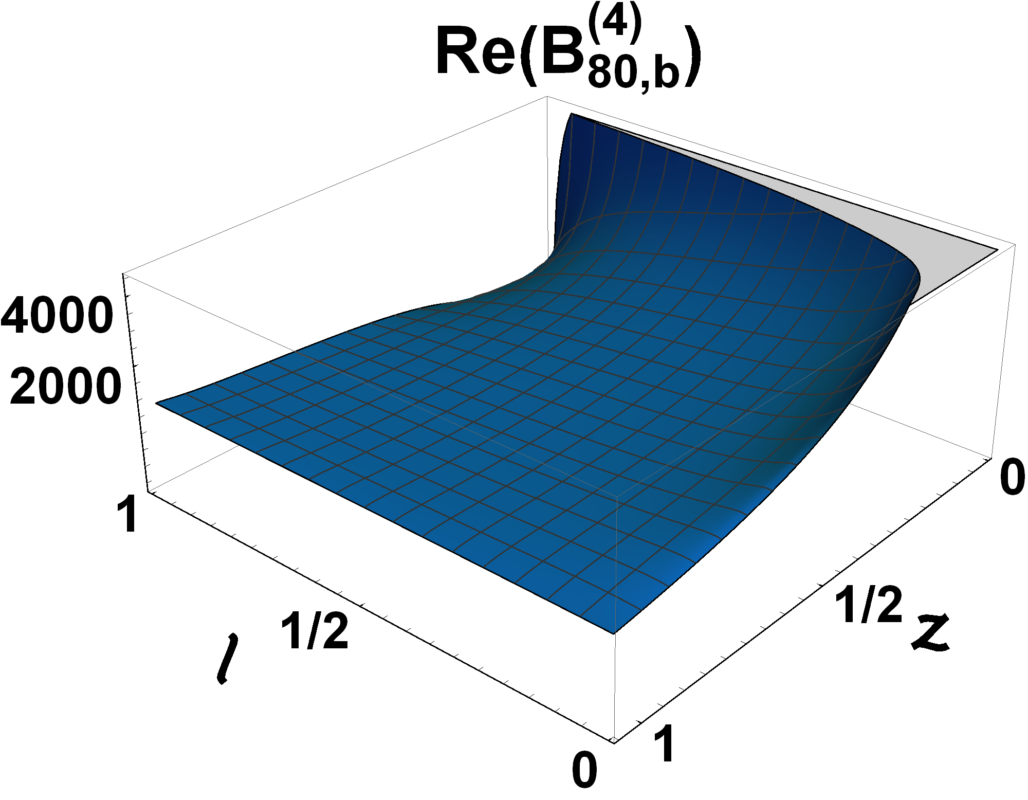
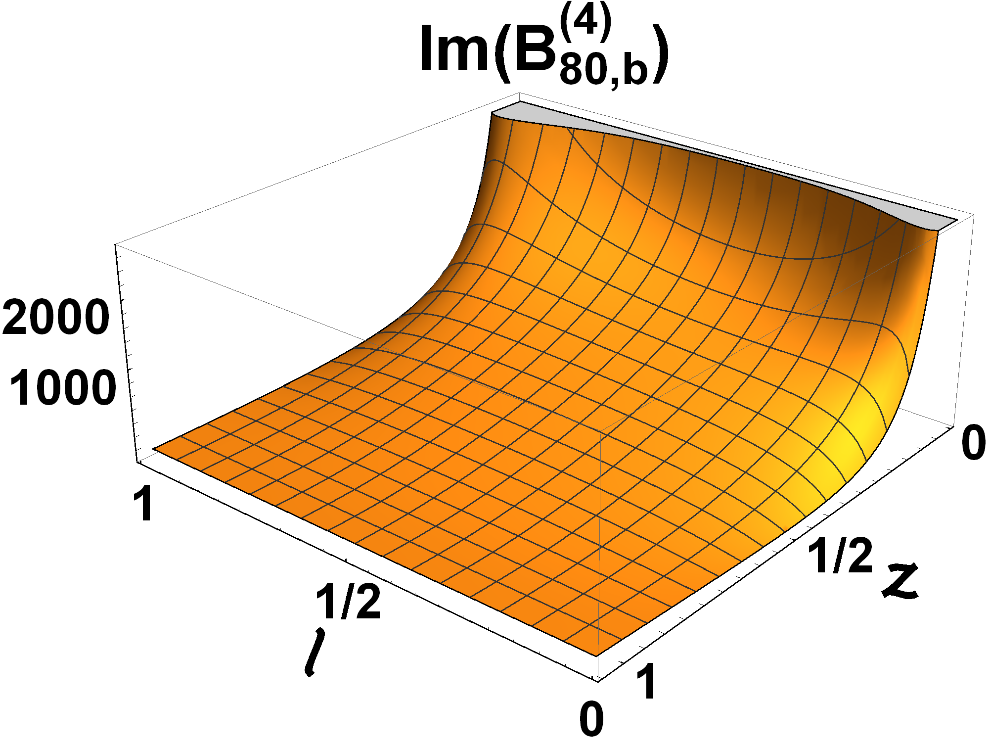
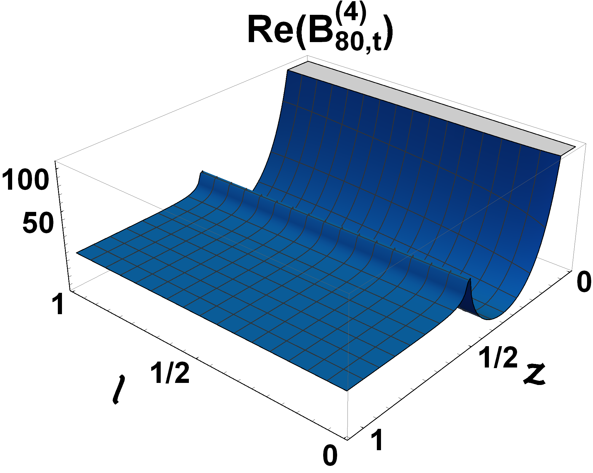
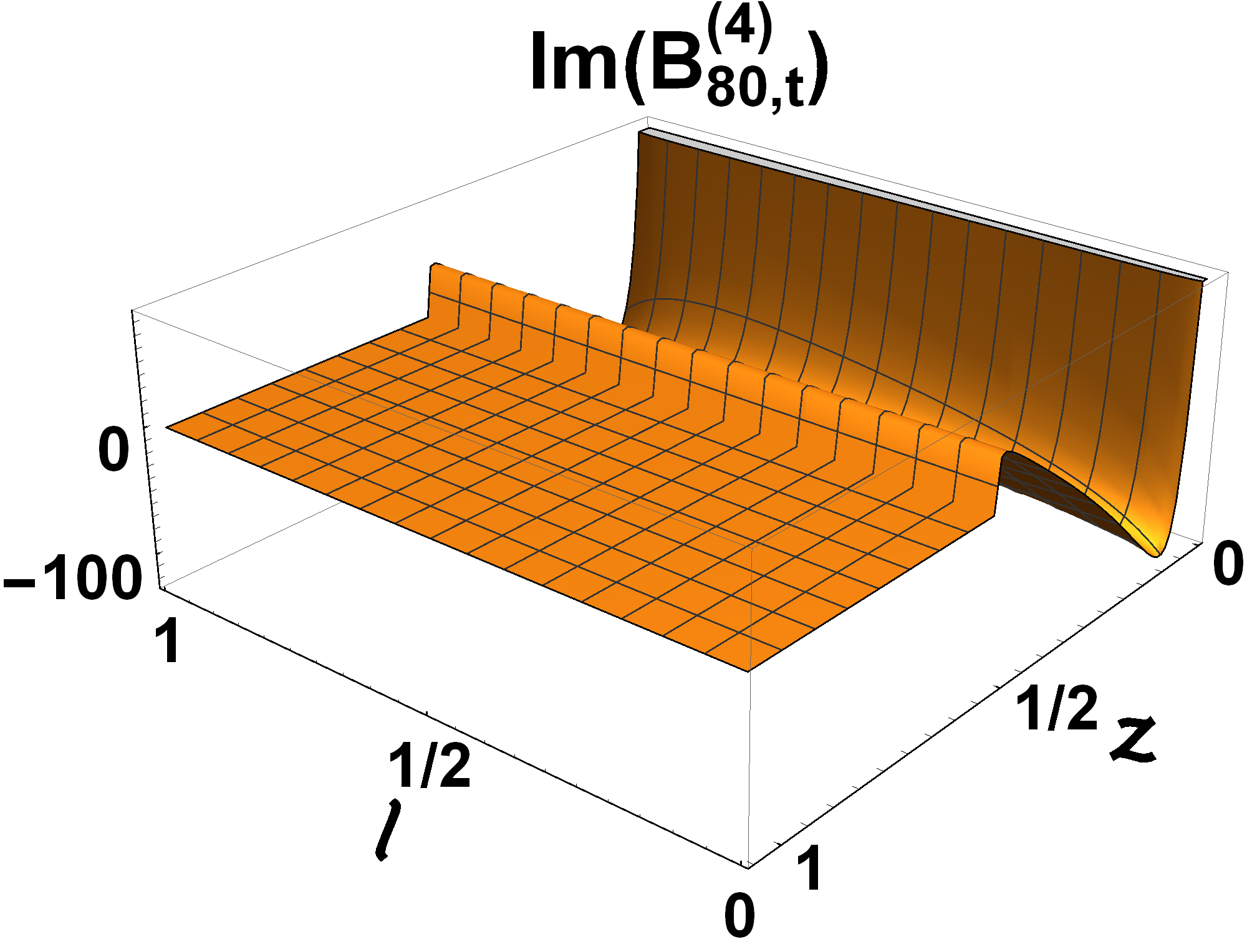
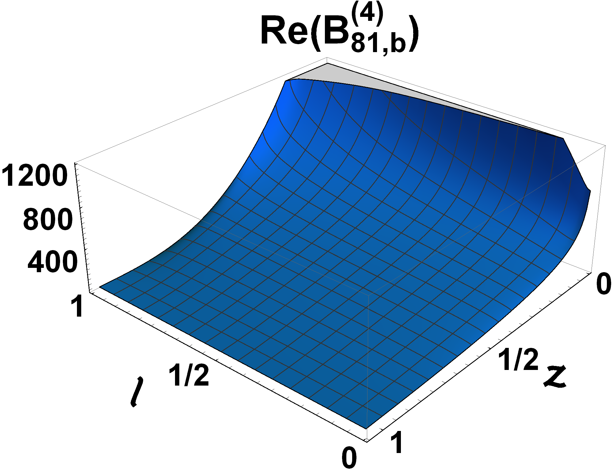
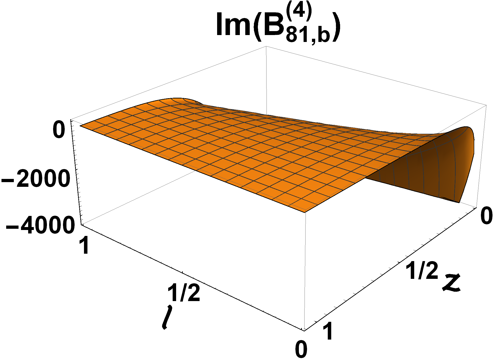
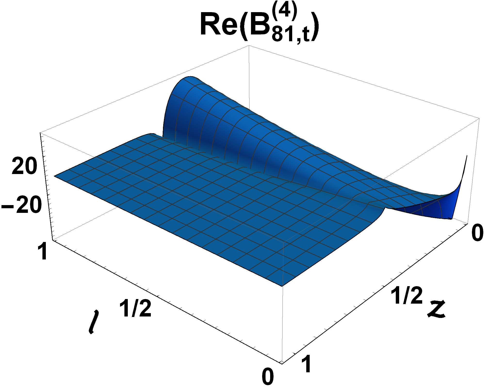
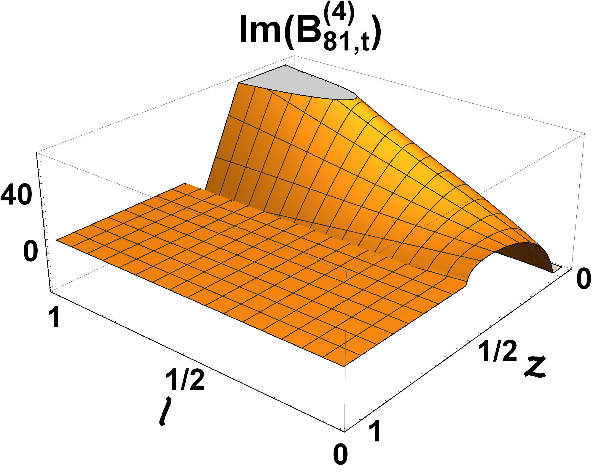
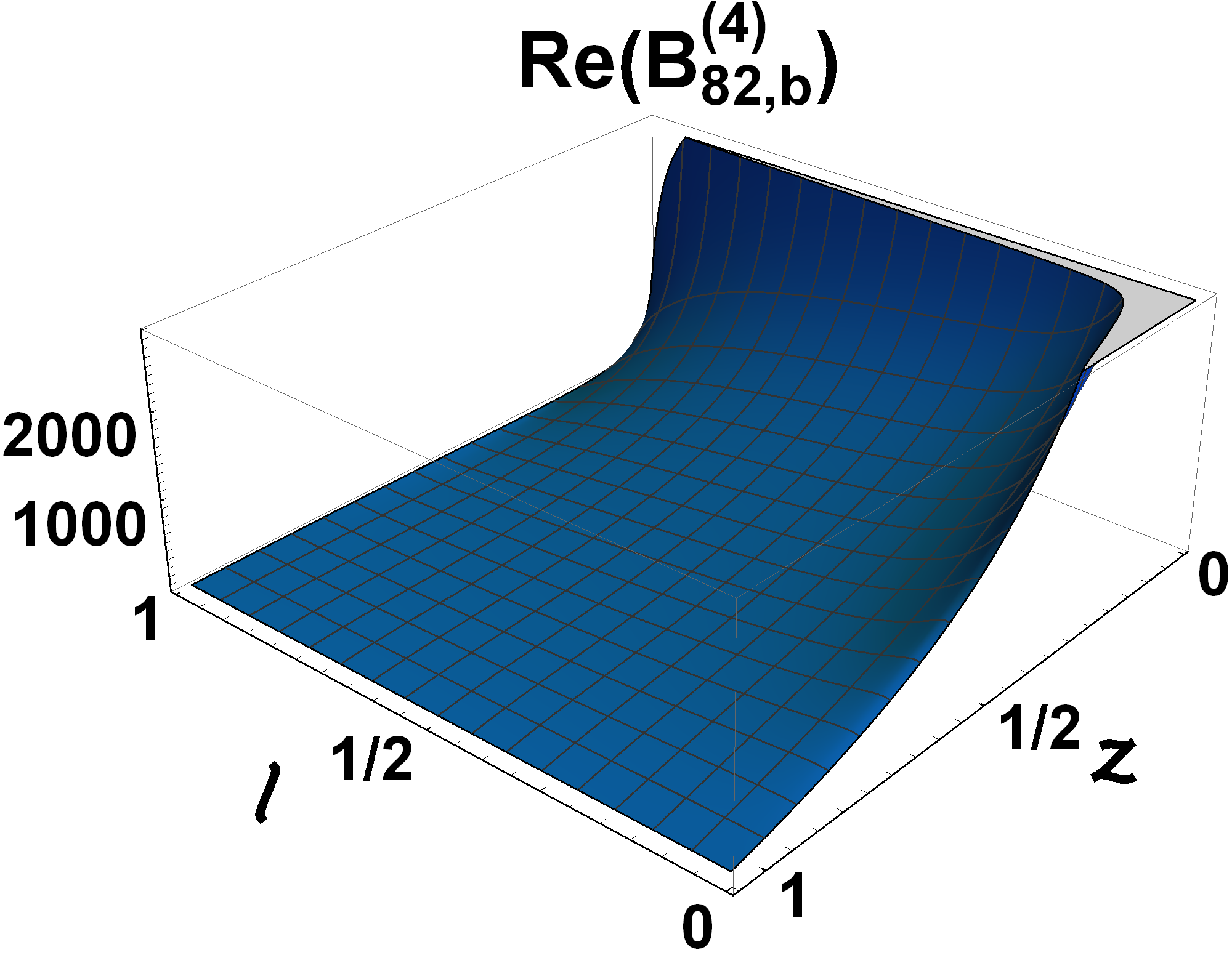
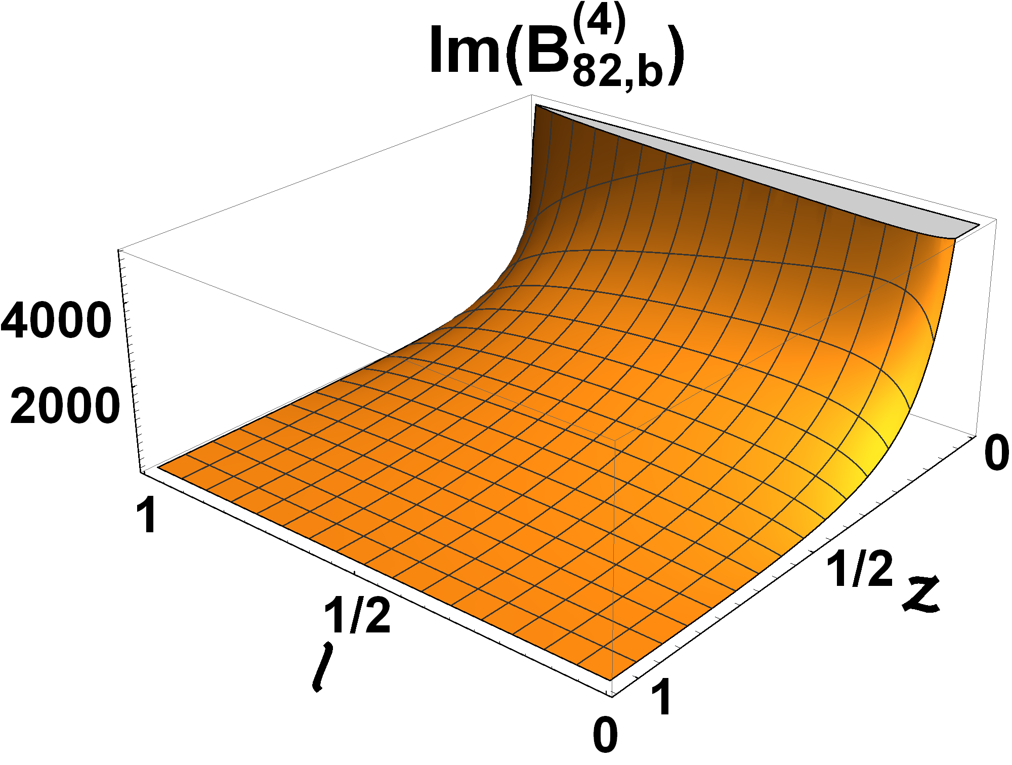
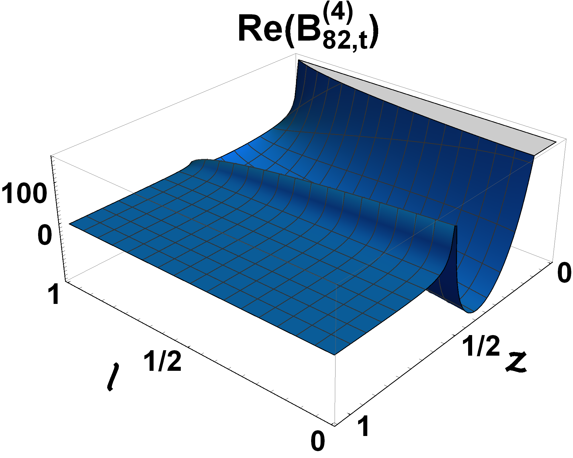
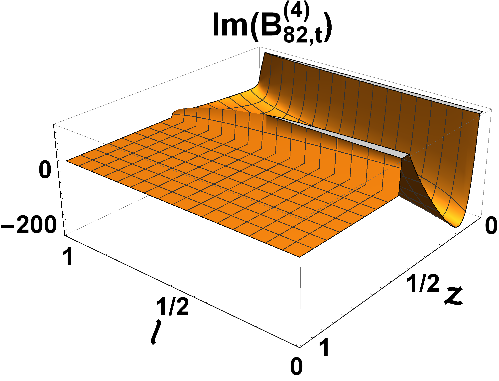
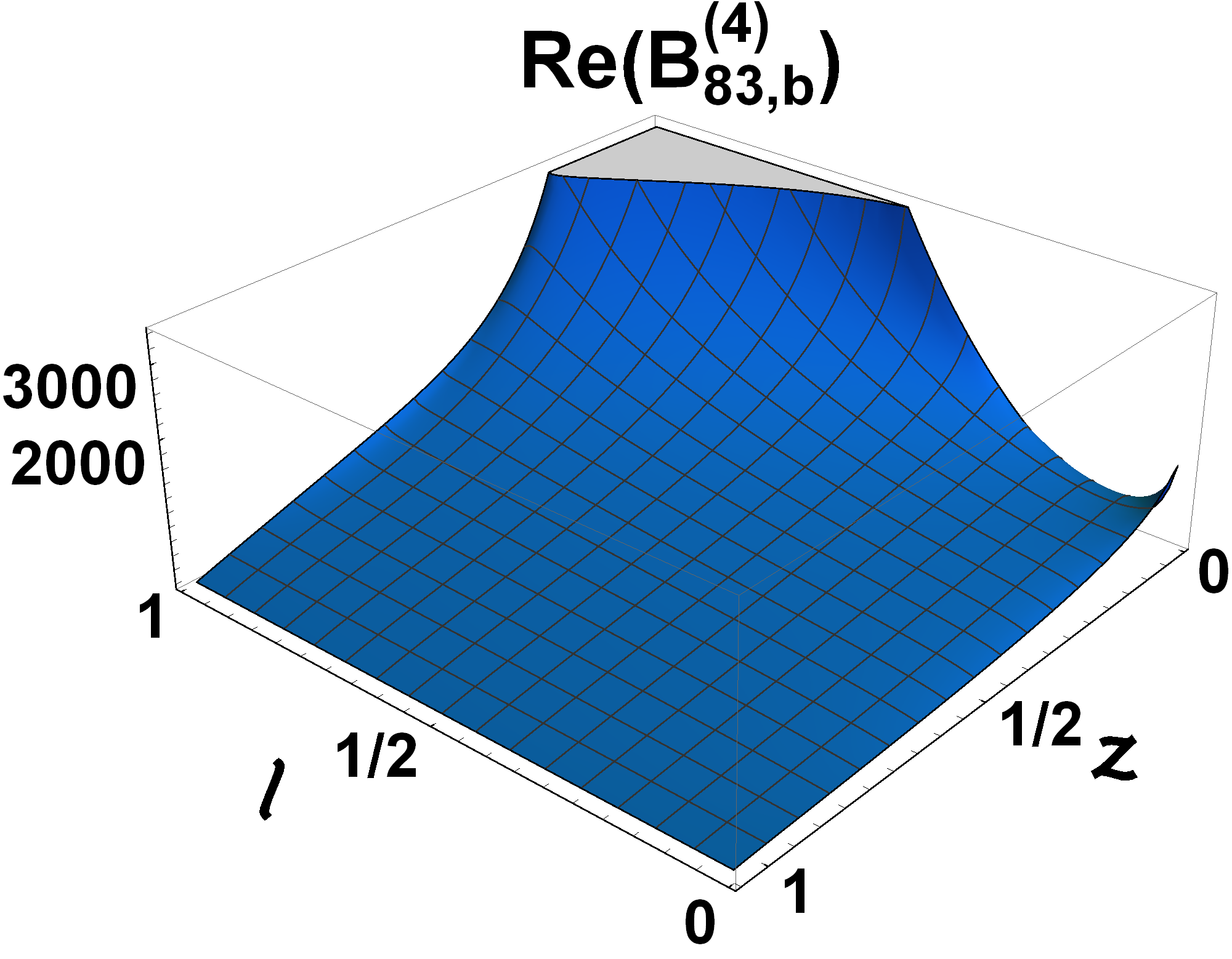
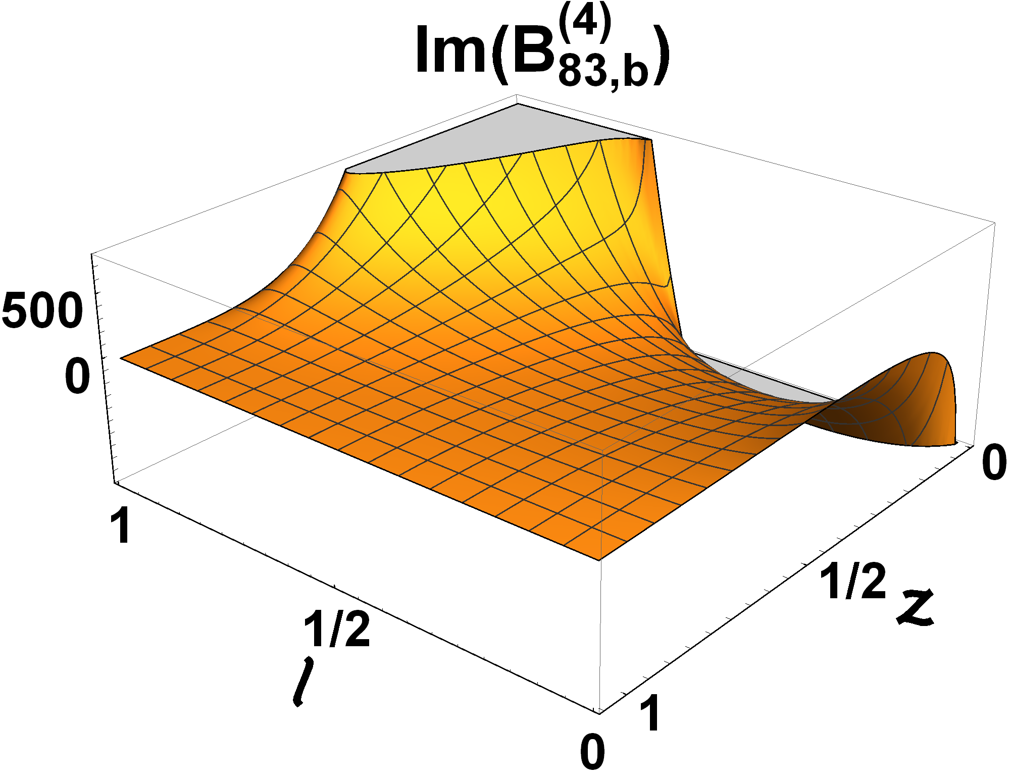
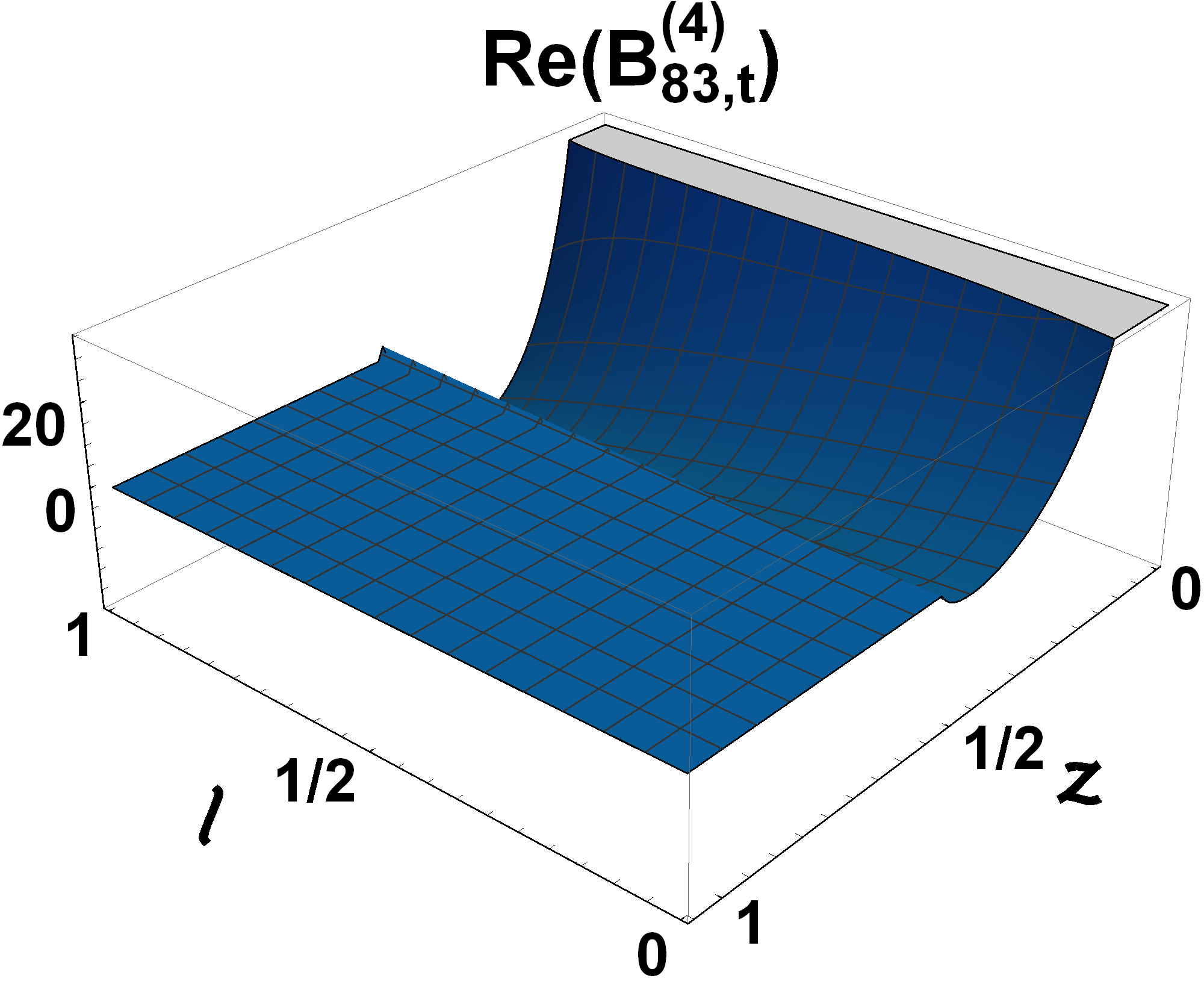
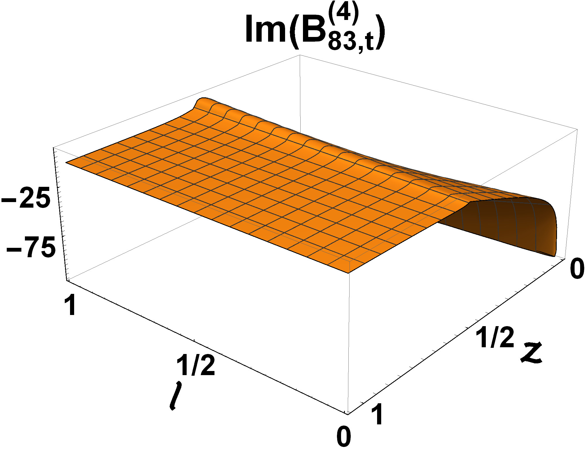
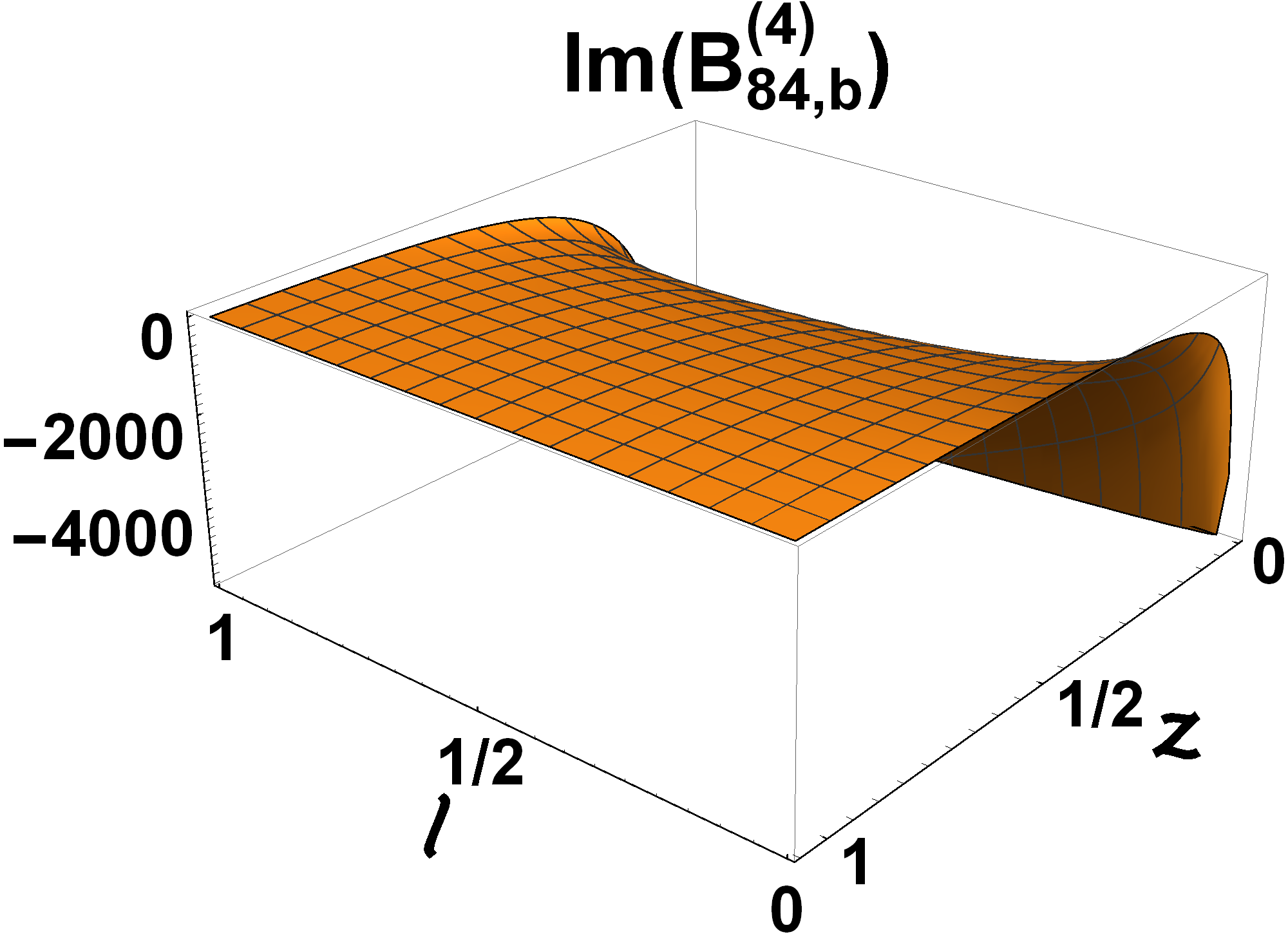
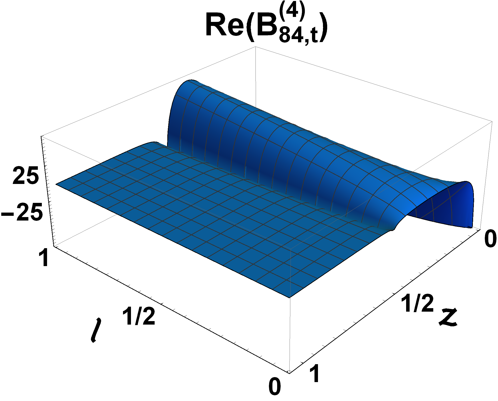
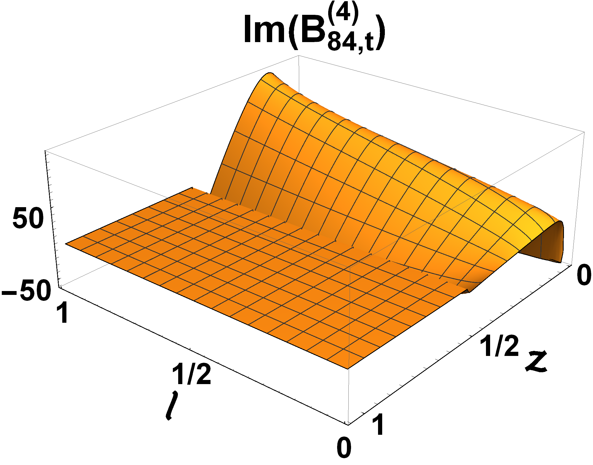
Figure 5: On the left (resp. right) are shown the real (blue) and imaginary (orange) part of the integrals of the top sector of Family G in the case of a virtual bottom (resp. top) quark running in the loop.

In this section we present explicit results that were obtained using the expansion method described in the previous section. Specifically, we used our method to compute the integrals in 100001000010000 points covering the physical region given below, for both the top- and bottom-quark corrections, and we present plots thereof. We compute the integrals in the physical region given by

s>0,t<0,s+tp42>0.formulae-sequence𝑠0formulae-sequence𝑡0𝑠𝑡superscriptsubscript𝑝420\displaystyle s>0\,,\quad t<0\,,\quad s+t-p_{4}^{2}>0\,. (36)

We may map that region to the unit square by using the parametrization,

s=p42z,t=p42l(z1)z.formulae-sequence𝑠superscriptsubscript𝑝42𝑧𝑡superscriptsubscript𝑝42𝑙𝑧1𝑧\displaystyle s=\frac{p_{4}^{2}}{z}\,,\quad t=\frac{p_{4}^{2}\,l\,(z-1)}{z}\,. (37)

Since we chose to work with m2=1superscript𝑚21m^{2}=1, the value for p42superscriptsubscript𝑝42p_{4}^{2} is given by mH2/mq2superscriptsubscript𝑚𝐻2superscriptsubscript𝑚𝑞2m_{H}^{2}/m_{q}^{2} where mHsubscript𝑚𝐻m_{H} denotes the mass of the Higgs particle, and mqsubscript𝑚𝑞m_{q} denotes the mass of the internal quark. For the top quark we approximate the ratio by p42=13/25superscriptsubscript𝑝421325p_{4}^{2}=13/25, while for the bottom quark we consider the ratio p42=323761/361superscriptsubscript𝑝42323761361p_{4}^{2}=323761/361.

For the case of the top quark, the particle production threshold s=4m2𝑠4superscript𝑚2s=4m^{2} corresponds to z=13/100𝑧13100z=13/100. For the sake of the presentation of the plots, we use a Möbius transformation to map z=13/100𝑧13100z=13/100 to 1/2121/2, while keeping z=0𝑧0z=0 and z=1𝑧1z=1 fixed. Thus, we consider the following parametrizations of the physical regions of the top and bottom quark contributions,

top(l,z)t:s\displaystyle\text{top}~{}~{}~{}(l,z)_{t}:\quad s =8774z25z,absent8774𝑧25𝑧\displaystyle=\frac{87-74z}{25z}\,,\, t=87l(z1)25z,𝑡87𝑙𝑧125𝑧\displaystyle t=\frac{87\,l\,(z-1)}{25z}\,,\, p42=1325,superscriptsubscript𝑝421325\displaystyle p_{4}^{2}=\frac{13}{25}\,,
bottom(l,z)b:s\displaystyle\text{bottom}~{}~{}~{}(l,z)_{b}:\quad s =323761361z,absent323761361𝑧\displaystyle=\frac{323761}{361z}\,,\, t=323761l(z1)361z,𝑡323761𝑙𝑧1361𝑧\displaystyle t=\frac{323761\,l\,(z-1)}{361z}\,,\, p42=323761361.superscriptsubscript𝑝42323761361\displaystyle p_{4}^{2}=\frac{323761}{361}\,. (38)

To produce plots in these regions we seek to compute n2superscript𝑛2n^{2} evenly spaced points on the unit square for all basis integrals, and in particular we let n=100𝑛100n=100, so that we obtain 10000 points in total. We explain next how we obtained results in these points. For convenience we use the notation ab𝑎𝑏a\rightarrow b to denote a line, we denote coordinates in the physical regions by pairs (l,z)𝑙𝑧(l,z), and we denote the heavy mass limit by 00\vec{0}. The following discussion applies to both the top and bottom region, given their respective set of (l,z)𝑙𝑧(l,z)-coordinates.

All of the results are derived using series expansions up to order 𝒪(λ50)𝒪superscript𝜆50\mathcal{O}(\lambda^{50}). First we set k=3𝑘3k=3, and move from the heavy mass limit to the point (1/(n+1),n/(n+1))1𝑛1𝑛𝑛1(1/(n+1),n/(n+1)). Then, we continue by moving along a vertical line (1/(n+1),n/(n+1))(1/(n+1),1/(n+1))1𝑛1𝑛𝑛11𝑛11𝑛1(1/(n+1),n/(n+1))\rightarrow(1/(n+1),1/(n+1)). This vertical line may be used to obtain values at the points (1/(n+1),y/(n+1))1𝑛1𝑦𝑛1(1/(n+1),y/(n+1)) for y=1,,n𝑦1𝑛y=1,\ldots,n. We may then consider n𝑛n horizontal lines (1/(n+1),x/(n+1))(n/(n+1),x/(n+1))1𝑛1𝑥𝑛1𝑛𝑛1𝑥𝑛1(1/(n+1),x/(n+1))\rightarrow(n/(n+1),x/(n+1)) for x=1,,n𝑥1𝑛x=1,\ldots,n, to obtain values at the points (x/(n+1),y/(n+1))𝑥𝑛1𝑦𝑛1(x/(n+1),y/(n+1)), for x,y=1,,nformulae-sequence𝑥𝑦1𝑛x,y=1,\ldots,n. The situation is depicted in Fig. 4, for the simpler case where n=10𝑛10n=10. We computed the expansions along the horizontal lines with k=2𝑘2k=2, in order to reduce the number of line segments needed and to save computation time. By working with k=3𝑘3k=3 for the first two lines, we made sure that the precision of the expansions along the horizontal lines is not limited by the precision of the expansions along the first two lines.

The resulting plots of integrals B80B84subscript𝐵80subscript𝐵84B_{80}-B_{84} for the top- and the bottom-quark are provided in Fig. 5. Note that as l𝑙l and z𝑧z range from zero to one, we travel across the full physical region defined in Eq. (36). For the plots we let n=100𝑛100n=100, and therefore the variables l𝑙l and z𝑧z range from 1/10111011/101 to 100/101100101100/101. Thus, in the plots a small part of the physical region is cut off at the boundary. In terms of the variables s𝑠s and t𝑡t, the plotted regions are given by:

top::topabsent\displaystyle\text{top}:~{}~{}~{} (13872500s871325)(52101100101st132525s101),13872500𝑠87132552101100101𝑠𝑡132525𝑠101\displaystyle\left(\frac{1387}{2500}\leq s\leq\frac{8713}{25}\right)\cup\left(\frac{52}{101}-\frac{100}{101}s\leq t\leq\frac{13}{2525}-\frac{s}{101}\right)\,,
bottom::bottomabsent\displaystyle\text{bottom}:~{}~{}~{} (3269986136100s32699861361)(3237610036461100101st32376136461s101).3269986136100𝑠326998613613237610036461100101𝑠𝑡32376136461𝑠101\displaystyle\left(\frac{32699861}{36100}\leq s\leq\frac{32699861}{361}\right)\cup\left(\frac{32376100}{36461}-\frac{100}{101}s\leq t\leq\frac{323761}{36461}-\frac{s}{101}\right)\,. (39)

Note that it is also possible to obtain numerical samples at points on the boundary of the physical region where the integrals are finite, see for example Ref. Abreu:2020jxa .

We computed the boundary data for the horizontal lines of the top and bottom physical regions on a laptop using a single core. We computed all horizontal lines on a cluster with 48 cores. The run for the horizontal lines of the top quark and the run for the horizontal lines of the bottom quark, both took a few hours to complete on the cluster.

5.1 Cross-checks of the expansions

We have performed several checks of our results. The first class of cross-checks was performed by evaluating multiple points by reaching them along different contours. The error that is accumulated while transporting results is different based on the chosen contour. Therefore, the difference of the results obtained through different contours gives a very good estimate of the precision of the results. In Table 1 we present the results of a number of cross-checks that were performed in this way. The maximum relative error that we encountered among all the points that were checked, is of order 𝒪(1025)𝒪superscript1025\mathcal{O}(10^{-25}), indicating that the results are valid up to at least 25 significant digits.

Line(s). Evaluated at #Segments (k=2)𝑘2(k=2) Max relative error
0(1101,1101)t0subscript11011101𝑡\vec{0}\rightarrow\left(\frac{1}{101},\frac{1}{101}\right)_{t} Endpoint 16 𝒪(1028)𝒪superscript1028\mathcal{O}(10^{-28})
0(1101,1101)b0subscript11011101𝑏\vec{0}\rightarrow\left(\frac{1}{101},\frac{1}{101}\right)_{b} Endpoint 31 𝒪(1026)𝒪superscript1026\mathcal{O}(10^{-26})
0(s=53t=11p42=23)(100101,45101)b0𝑠53𝑡11superscriptsubscript𝑝4223subscript10010145101𝑏\vec{0}\rightarrow\,\left(\begin{smallmatrix}s=53\\ t=-11\\ p_{4}^{2}=23\end{smallmatrix}\right)\rightarrow\left(\frac{100}{101},\frac{45}{101}\right)_{b} Endpoint 47 𝒪(1025)𝒪superscript1025\mathcal{O}(10^{-25})
(x101,100101)t(x101,1101)tfor x=1,,100for 𝑥1100subscript𝑥101100101𝑡subscript𝑥1011101𝑡\underset{\text{for }\,x=1,\ldots,100}{\left(\frac{x}{101},\frac{100}{101}\right)_{t}\rightarrow\left(\frac{x}{101},\frac{1}{101}\right)_{t}} (x101,y101)tfor x,y=1,,100formulae-sequencefor 𝑥𝑦1100subscript𝑥101𝑦101𝑡\underset{\text{for }\,x,y=1,\ldots,100}{\left(\frac{x}{101},\frac{y}{101}\right)_{t}} 2568 𝒪(1025)𝒪superscript1025\mathcal{O}(10^{-25})
(45101,45101)b(1101,100101)tsubscript4510145101𝑏subscript1101100101𝑡\left(\frac{45}{101},\frac{45}{101}\right)_{b}\rightarrow\left(\frac{1}{101},\frac{100}{101}\right)_{t} Endpoint 21 𝒪(1027)𝒪superscript1027\mathcal{O}(10^{-27})
Table 1: This table presents a number of internal cross-checks of our results. In the first column we give additional lines along which we computed results, different from the lines in Fig. 4. These results were then compared to the results that we generated for the plots, which were computed in the manner illustrated in Fig. 4. For the lines starting from 00\vec{0}, we fixed the boundary conditions in the heavy mass limit, while for the lines in the last two rows we fixed the boundary conditions from the results that we generated for the plots. In the last column we give highest value of the relative error |Bi,cross-check(ϵ-order)/Bi,plot(ϵ-order)|1superscriptsubscript𝐵𝑖cross-checkitalic-ϵ-ordersuperscriptsubscript𝐵𝑖plotitalic-ϵ-order1\left|B_{i,\text{cross-check}}^{(\epsilon\text{-order})}/B_{i,\text{plot}}^{(\epsilon\text{-order})}\right|-1 for all integrals i=1,,84𝑖184i=1,\ldots,84, and ϵitalic-ϵ\epsilon-orders 0 to 4.

For the top-quark integrals we compared our results against FIESTA Smirnov:2015mct for multiple points of the physical region finding full agreement within the Monte Carlo error reported by FIESTA. For the physical region of the bottom quark we checked most of the integrals against FIESTA and SecDec Borowka:2017idc . However, for some of the integrals, these programs encounter numerical instabilities. In those cases we have performed different checks. Firstly we cross checked our results against FIESTA in the point (s=53,t=11,p42=23,m2=1)formulae-sequence𝑠53formulae-sequence𝑡11formulae-sequencesuperscriptsubscript𝑝4223superscript𝑚21(s=53,\,t=-11,\,p_{4}^{2}=23,m^{2}=1) finding full agreement. This provides a direct check of the analytic continuation past the thresholds s=4m2𝑠4superscript𝑚2s=4m^{2} and p42=4m2superscriptsubscript𝑝424superscript𝑚2p_{4}^{2}=4m^{2}. In addition, we have performed a numerical cross-check against a private code Capatti:2019edf for the numerical evaluation of multi-loop integrals in momentum space using the loop tree duality Capatti:2019ypt (for related work on the loop tree duality see also Catani:2008xa ; Aguilera-Verdugo:2019kbz ; Bierenbaum:2010cy ; Runkel:2019yrs ). In particular, we compared integrals B72subscript𝐵72B_{72} and B76subscript𝐵76B_{76} in the point (10/101,10/101)b=(s=32699861/3610,t=29462251/36461,p42=323761/361,m2=1)subscript1010110101𝑏formulae-sequence𝑠326998613610formulae-sequence𝑡2946225136461formulae-sequencesuperscriptsubscript𝑝42323761361superscript𝑚21(10/101,10/101)_{b}=(s=32699861/3610,t=-29462251/36461,p_{4}^{2}=323761/361,m^{2}=1) finding full agreement. Lastly, for one of the internal cross-checks we transported the results for the bottom-quark integrals from the point (45101,45101)bsubscript4510145101𝑏\left(\frac{45}{101},\frac{45}{101}\right)_{b} along a straight line to the point (1101,100101)tsubscript1101100101𝑡\left(\frac{1}{101},\frac{100}{101}\right)_{t}. We compared this to the results that were obtained in the point (1101,100101)tsubscript1101100101𝑡\left(\frac{1}{101},\frac{100}{101}\right)_{t} by transporting directly from the heavy mass limit, and found a relative deviation of 𝒪(1027)𝒪superscript1027\mathcal{O}(10^{-27}). This cross-check is indicated by the last row in Table 1.

6 Conclusion

In this paper we computed a family of two-loop non-planar master integrals relevant for the QCD corrections to Higgs plus one jet production in the full theory. Our result, together with Bonciani:2016qxi ; Bonciani:2019jyb ; Francesco:2019yqt , provide the full set of master integrals required for the computation of the NLO corrections to Higgs plus one jet production, and the NLO corrections to the pTsubscript𝑝𝑇p_{T} distribution of the Higgs. Moreover, our results provide the full set of master integrals relevant for the NLO corrections to Higgs decay to three partons, and the single-real radiation contributions to the NNLO corrections to inclusive Higgs production.

The computation was performed by using the differential equations method. More specifically, we defined an integral basis such that most of the integrals satisfy differential equations in canonical form. Three integral sectors are coupled, and their solution involve functions of elliptic type. Having phenomenological applications in mind, we solved the differential equations along contours in the space of kinematic invariants, in terms of one-dimensional generalized power series. More specifically, given a boundary point where the value of the integrals is known, we defined the differential equations along a contour connecting a boundary point to a new point of the kinematic regions. In this way the problem was effectively reduced to one with a single scale, and finding the series solution was algorithmic. We showed that this method is efficient, and can be repeated in order to compute the integrals in any point of the kinematic regions. The analytic continuation of the series solution across the physical thresholds is straightforward, as it requires only the analytic continuation of logarithms and square roots.

In order to show the generality of our approach, we computed the master integrals for both the top- and bottom-quark mass. Moreover, we explicitly obtained results for a large set of points covering our physical regions. The typical evaluation time is of the order of 111 second per integral, with a relative accuracy of order 1024superscript102410^{-24}, on a single CPU core. If needed, the numerical precision can be made arbitrarily high by increasing the truncation order of the power series. These features render our methods well suited for Monte Carlo phase-space integrations.

We remark that the applicability of our methods does not rely on the number of physical scales, specific kinematic configurations, or a particular form of the differential equations, and a public implementation has been recently developed in Hidding:2020ytt . For this reasons, we believe that our approach will be relevant for the computation of several processes of phenomenological interest.

Acknowledgements

The authors would like to thank Zeno Capatti and Valentin Hirschi for performing cross checks of our results against a private code for the numerical evaluation of multi-loop integrals using the loop tree duality. We thank Roberto Bonciani, Vittorio Del Duca, Johannes Henn and Volodya Smirnov for useful discussions and collaboration on related work. The work of HF is part of the HiProLoop project funded by the European Union’s Horizon 2020 research and innovation programme under the Marie Skłodowska-Curie grant agreement 747178. The work of FM was funded by the European Research Council (ERC) under grant agreement No. 694712 (pertQCD) and by the Swiss National Science Foundation project No. 177632 (ElliptHiggs). The work of MH was funded by the European Research Council (ERC) under grant agreement No. 647356 (CutLoops). The work of LM received funding from the European Research Council (ERC) under the European Union’s Horizon 2020 research and innovation programme, Novel structures in scattering amplitudes (grant agreement No. 725110). GS is supported by the Simons Investigator Award ##{\#}376208 of A. Volovich. MH, LM and GS would like to thank ETH Zurich for hospitality during the preparation of this work.

Appendix A Canonical basis and basis for elliptic sectors

In this section we provide the set of 84 basis integrals used in this paper, written in terms of the set of master integrals depicted in Figure 2 and defined as in Eq. (1).

The canonical basis for the first 71 integrals is,

B1subscript𝐵1\displaystyle B_{1} =ϵ2I0,2,0,0,2,0,0,0,0,absentsuperscriptitalic-ϵ2subscriptI020020000\displaystyle=\epsilon^{2}\text{I}_{0,2,0,0,2,0,0,0,0}\,,
B2subscript𝐵2\displaystyle B_{2} =ϵ2r2r6I0,2,0,0,2,0,1,0,0,absentsuperscriptitalic-ϵ2subscript𝑟2subscript𝑟6subscriptI020020100\displaystyle=\epsilon^{2}r_{2}r_{6}\text{I}_{0,2,0,0,2,0,1,0,0}\,,
B3subscript𝐵3\displaystyle B_{3} =ϵ2r1r5I0,2,0,1,0,2,0,0,0,absentsuperscriptitalic-ϵ2subscript𝑟1subscript𝑟5subscriptI020102000\displaystyle=\epsilon^{2}r_{1}r_{5}\text{I}_{0,2,0,1,0,2,0,0,0}\,,
B4subscript𝐵4\displaystyle B_{4} =ϵ2sI1,2,0,0,2,0,0,0,0,absentsuperscriptitalic-ϵ2𝑠subscriptI120020000\displaystyle=\epsilon^{2}s\text{I}_{1,2,0,0,2,0,0,0,0}\,,
B5subscript𝐵5\displaystyle B_{5} =ϵ2r2r6(12I1,2,0,0,2,0,0,0,0+I2,2,0,0,1,0,0,0,0),absentsuperscriptitalic-ϵ2subscript𝑟2subscript𝑟612subscriptI120020000subscriptI220010000\displaystyle=\epsilon^{2}r_{2}r_{6}\left(\frac{1}{2}\text{I}_{1,2,0,0,2,0,0,0,0}+\text{I}_{2,2,0,0,1,0,0,0,0}\right)\,,
B6subscript𝐵6\displaystyle B_{6} =ϵ2tI0,2,1,0,0,2,0,0,0,absentsuperscriptitalic-ϵ2𝑡subscriptI021002000\displaystyle=\epsilon^{2}t\text{I}_{0,2,1,0,0,2,0,0,0}\,,
B7subscript𝐵7\displaystyle B_{7} =ϵ2r3r7(12I0,2,1,0,0,2,0,0,0+I0,2,2,0,0,1,0,0,0),absentsuperscriptitalic-ϵ2subscript𝑟3subscript𝑟712subscriptI021002000subscriptI022001000\displaystyle=\epsilon^{2}r_{3}r_{7}\left(\frac{1}{2}\text{I}_{0,2,1,0,0,2,0,0,0}+\text{I}_{0,2,2,0,0,1,0,0,0}\right)\,,
B8subscript𝐵8\displaystyle B_{8} =ϵ2(p42st)I1,0,0,2,0,2,0,0,0,absentsuperscriptitalic-ϵ2superscriptsubscript𝑝42𝑠𝑡subscriptI100202000\displaystyle=\epsilon^{2}(p_{4}^{2}-s-t)\text{I}_{1,0,0,2,0,2,0,0,0}\,,
B9subscript𝐵9\displaystyle B_{9} =ϵ2r4r8(12I1,0,0,2,0,2,0,0,0+I2,0,0,1,0,2,0,0,0),absentsuperscriptitalic-ϵ2subscript𝑟4subscript𝑟812subscriptI100202000subscriptI200102000\displaystyle=\epsilon^{2}r_{4}r_{8}\left(\frac{1}{2}\text{I}_{1,0,0,2,0,2,0,0,0}+\text{I}_{2,0,0,1,0,2,0,0,0}\right)\,,
B10subscript𝐵10\displaystyle B_{10} =ϵ2p42I0,2,1,0,2,0,0,0,0,absentsuperscriptitalic-ϵ2superscriptsubscript𝑝42subscriptI021020000\displaystyle=\epsilon^{2}p_{4}^{2}\text{I}_{0,2,1,0,2,0,0,0,0}\,,
B11subscript𝐵11\displaystyle B_{11} =ϵ2r1r5(12I0,2,1,0,2,0,0,0,0+I0,2,2,0,1,0,0,0,0),absentsuperscriptitalic-ϵ2subscript𝑟1subscript𝑟512subscriptI021020000subscriptI022010000\displaystyle=\epsilon^{2}r_{1}r_{5}\left(\frac{1}{2}\text{I}_{0,2,1,0,2,0,0,0,0}+\text{I}_{0,2,2,0,1,0,0,0,0}\right)\,,
B12subscript𝐵12\displaystyle B_{12} =ϵ3sI0,2,0,0,1,1,1,0,0,absentsuperscriptitalic-ϵ3𝑠subscriptI020011100\displaystyle=\epsilon^{3}s\text{I}_{0,2,0,0,1,1,1,0,0}\,,
B13subscript𝐵13\displaystyle B_{13} =ϵ2r1r2r5r6I0,2,0,1,2,0,1,0,0,absentsuperscriptitalic-ϵ2subscript𝑟1subscript𝑟2subscript𝑟5subscript𝑟6subscriptI020120100\displaystyle=-\epsilon^{2}r_{1}r_{2}r_{5}r_{6}\text{I}_{0,2,0,1,2,0,1,0,0}\,,
B14subscript𝐵14\displaystyle B_{14} =ϵ3sI1,2,0,0,1,1,0,0,0,absentsuperscriptitalic-ϵ3𝑠subscriptI120011000\displaystyle=\epsilon^{3}s\text{I}_{1,2,0,0,1,1,0,0,0}\,,
B15subscript𝐵15\displaystyle B_{15} =ϵ3tI0,2,1,0,0,1,1,0,0,absentsuperscriptitalic-ϵ3𝑡subscriptI021001100\displaystyle=\epsilon^{3}t\text{I}_{0,2,1,0,0,1,1,0,0}\,,
B16subscript𝐵16\displaystyle B_{16} =ϵ3(p42st)I1,0,0,2,1,1,0,0,0,absentsuperscriptitalic-ϵ3superscriptsubscript𝑝42𝑠𝑡subscriptI100211000\displaystyle=\epsilon^{3}(p_{4}^{2}-s-t)\text{I}_{1,0,0,2,1,1,0,0,0}\,,
B17subscript𝐵17\displaystyle B_{17} =ϵ3(p42t)I0,2,1,0,1,1,0,0,0,absentsuperscriptitalic-ϵ3superscriptsubscript𝑝42𝑡subscriptI021011000\displaystyle=\epsilon^{3}(p_{4}^{2}-t)\text{I}_{0,2,1,0,1,1,0,0,0}\,,
B18subscript𝐵18\displaystyle B_{18} =ϵ3(s+t)I1,0,0,2,0,1,1,0,0,absentsuperscriptitalic-ϵ3𝑠𝑡subscriptI100201100\displaystyle=\epsilon^{3}(s+t)\text{I}_{1,0,0,2,0,1,1,0,0}\,,
B19subscript𝐵19\displaystyle B_{19} =ϵ3(sp42)I0,2,1,0,1,0,1,0,0,absentsuperscriptitalic-ϵ3𝑠superscriptsubscript𝑝42subscriptI021010100\displaystyle=\epsilon^{3}(s-p_{4}^{2})\text{I}_{0,2,1,0,1,0,1,0,0}\,,
B20subscript𝐵20\displaystyle B_{20} =ϵ2m2(sp42)I0,3,1,0,1,0,1,0,0,absentsuperscriptitalic-ϵ2superscript𝑚2𝑠superscriptsubscript𝑝42subscriptI031010100\displaystyle=\epsilon^{2}m^{2}(s-p_{4}^{2})\text{I}_{0,3,1,0,1,0,1,0,0}\,,
B21subscript𝐵21\displaystyle B_{21} =ϵ2r2r64(s2p42)(4(m2s+p44p42s)I0,2,1,0,2,0,1,0,0+\displaystyle=\epsilon^{2}\frac{r_{2}r_{6}}{4(s-2p_{4}^{2})}\left(4\left(m^{2}s+p_{4}^{4}-p_{4}^{2}s\right)\text{I}_{0,2,1,0,2,0,1,0,0}+\right.
+4m2(sp42)I0,3,1,0,1,0,1,0,0+6ϵ(p42s)I0,2,1,0,1,0,1,0,03p42I0,2,1,0,2,0,0,0,0),\displaystyle+\left.4m^{2}(s-p_{4}^{2})\text{I}_{0,3,1,0,1,0,1,0,0}+6\epsilon(p_{4}^{2}-s)\text{I}_{0,2,1,0,1,0,1,0,0}-3p_{4}^{2}\text{I}_{0,2,1,0,2,0,0,0,0}\right)\,,
B22subscript𝐵22\displaystyle B_{22} =ϵ3(p42s)I1,1,0,1,2,0,0,0,0,absentsuperscriptitalic-ϵ3superscriptsubscript𝑝42𝑠subscriptI110120000\displaystyle=\epsilon^{3}(p_{4}^{2}-s)\text{I}_{1,1,0,1,2,0,0,0,0}\,,
B23subscript𝐵23\displaystyle B_{23} =ϵ2m2(p42s)I1,1,0,1,3,0,0,0,0,absentsuperscriptitalic-ϵ2superscript𝑚2superscriptsubscript𝑝42𝑠subscriptI110130000\displaystyle=\epsilon^{2}m^{2}(p_{4}^{2}-s)\text{I}_{1,1,0,1,3,0,0,0,0}\,,
B24subscript𝐵24\displaystyle B_{24} =ϵ2r1r54(p422s)(4m2I1,1,0,1,3,0,0,0,0(p42s)+4m2p42I1,2,0,1,2,0,0,0,0+\displaystyle=\epsilon^{2}\frac{r_{1}r_{5}}{4(p_{4}^{2}-2s)}\left(4m^{2}\text{I}_{1,1,0,1,3,0,0,0,0}(p_{4}^{2}-s)+4m^{2}p_{4}^{2}\text{I}_{1,2,0,1,2,0,0,0,0}\right.+
+6ϵ(sp42)I1,1,0,1,2,0,0,0,04p42sI1,2,0,1,2,0,0,0,0+6italic-ϵ𝑠superscriptsubscript𝑝42subscriptI110120000limit-from4superscriptsubscript𝑝42𝑠subscriptI120120000\displaystyle\left.+6\epsilon(s-p_{4}^{2})\text{I}_{1,1,0,1,2,0,0,0,0}-4p_{4}^{2}s\text{I}_{1,2,0,1,2,0,0,0,0}+\right.
+4s2I1,2,0,1,2,0,0,0,03sI1,2,0,0,2,0,0,0,0),\displaystyle+\left.4s^{2}\text{I}_{1,2,0,1,2,0,0,0,0}-3s\text{I}_{1,2,0,0,2,0,0,0,0}\right)\,,
B25subscript𝐵25\displaystyle B_{25} =ϵ3(p42t)I0,1,1,1,0,2,0,0,0,absentsuperscriptitalic-ϵ3superscriptsubscript𝑝42𝑡subscriptI011102000\displaystyle=\epsilon^{3}(p_{4}^{2}-t)\text{I}_{0,1,1,1,0,2,0,0,0}\,,
B26subscript𝐵26\displaystyle B_{26} =ϵ2m2(p42t)I0,1,1,1,0,3,0,0,0,absentsuperscriptitalic-ϵ2superscript𝑚2superscriptsubscript𝑝42𝑡subscriptI011103000\displaystyle=\epsilon^{2}m^{2}(p_{4}^{2}-t)\text{I}_{0,1,1,1,0,3,0,0,0}\,,
B27subscript𝐵27\displaystyle B_{27} =ϵ2r1r54(p422t)(4m2(p42t)I0,1,1,1,0,3,0,0,0+4m2p42I0,2,1,1,0,2,0,0,0\displaystyle=\epsilon^{2}\frac{r_{1}r_{5}}{4(p_{4}^{2}-2t)}\left(4m^{2}(p_{4}^{2}-t)\text{I}_{0,1,1,1,0,3,0,0,0}+4m^{2}p_{4}^{2}\text{I}_{0,2,1,1,0,2,0,0,0}\right.
+6ϵ(tp42)I0,1,1,1,0,2,0,0,04p42tI0,2,1,1,0,2,0,0,0+6italic-ϵ𝑡superscriptsubscript𝑝42subscriptI011102000limit-from4superscriptsubscript𝑝42𝑡subscriptI021102000\displaystyle+\left.6\epsilon(t-p_{4}^{2})\text{I}_{0,1,1,1,0,2,0,0,0}-4p_{4}^{2}t\text{I}_{0,2,1,1,0,2,0,0,0}+\right.
+4t2I0,2,1,1,0,2,0,0,03tI0,2,1,0,0,2,0,0,0),\displaystyle+\left.4t^{2}\text{I}_{0,2,1,1,0,2,0,0,0}-3t\text{I}_{0,2,1,0,0,2,0,0,0}\right)\,,
B28subscript𝐵28\displaystyle B_{28} =ϵ3(s+t)I1,1,0,1,0,2,0,0,0,absentsuperscriptitalic-ϵ3𝑠𝑡subscriptI110102000\displaystyle=\epsilon^{3}(s+t)\text{I}_{1,1,0,1,0,2,0,0,0}\,,
B29subscript𝐵29\displaystyle B_{29} =ϵ2m2(s+t)I1,1,0,1,0,3,0,0,0,absentsuperscriptitalic-ϵ2superscript𝑚2𝑠𝑡subscriptI110103000\displaystyle=\epsilon^{2}m^{2}(s+t)\text{I}_{1,1,0,1,0,3,0,0,0}\,,
B30subscript𝐵30\displaystyle B_{30} =ϵ2r1r54(p422(s+t))(4(m2p42(s+t)(p42st))I1,1,0,2,0,2,0,0,0\displaystyle=-\epsilon^{2}\frac{r_{1}r_{5}}{4(p_{4}^{2}-2(s+t))}\left(4(m^{2}p_{4}^{2}-(s+t)(p_{4}^{2}-s-t))\text{I}_{1,1,0,2,0,2,0,0,0}\right.
+4m2(s+t)I1,1,0,1,0,3,0,0,0+3(p42+s+t)I1,0,0,2,0,2,0,0,04superscript𝑚2𝑠𝑡subscriptI110103000limit-from3superscriptsubscript𝑝42𝑠𝑡subscriptI100202000\displaystyle+\left.4m^{2}(s+t)\text{I}_{1,1,0,1,0,3,0,0,0}+3(-p_{4}^{2}+s+t)\text{I}_{1,0,0,2,0,2,0,0,0}-\right.
6ϵ(s+t)I1,1,0,1,0,2,0,0,0),\displaystyle-\left.6\epsilon(s+t)\text{I}_{1,1,0,1,0,2,0,0,0}\right)\,,
B31subscript𝐵31\displaystyle B_{31} =ϵ3sr1r5I0,2,0,1,1,1,1,0,0,absentsuperscriptitalic-ϵ3𝑠subscript𝑟1subscript𝑟5subscriptI020111100\displaystyle=\epsilon^{3}sr_{1}r_{5}\text{I}_{0,2,0,1,1,1,1,0,0}\,,
B32subscript𝐵32\displaystyle B_{32} =ϵ4(p42t)I0,1,1,1,1,1,0,0,0,absentsuperscriptitalic-ϵ4superscriptsubscript𝑝42𝑡subscriptI011111000\displaystyle=\epsilon^{4}(p_{4}^{2}-t)\text{I}_{0,1,1,1,1,1,0,0,0}\,,
B33subscript𝐵33\displaystyle B_{33} =ϵ3(p42t)r1r5I0,2,1,1,1,1,0,0,0,absentsuperscriptitalic-ϵ3superscriptsubscript𝑝42𝑡subscript𝑟1subscript𝑟5subscriptI021111000\displaystyle=\epsilon^{3}(p_{4}^{2}-t)r_{1}r_{5}\text{I}_{0,2,1,1,1,1,0,0,0}\,,
B34subscript𝐵34\displaystyle B_{34} =ϵ4(s+t)I1,1,0,1,0,1,1,0,0,absentsuperscriptitalic-ϵ4𝑠𝑡subscriptI110101100\displaystyle=\epsilon^{4}(s+t)\text{I}_{1,1,0,1,0,1,1,0,0}\,,
B35subscript𝐵35\displaystyle B_{35} =ϵ3(s+t)r1r5I1,1,0,2,0,1,1,0,0,absentsuperscriptitalic-ϵ3𝑠𝑡subscript𝑟1subscript𝑟5subscriptI110201100\displaystyle=\epsilon^{3}(s+t)r_{1}r_{5}\text{I}_{1,1,0,2,0,1,1,0,0}\,,
B36subscript𝐵36\displaystyle B_{36} =ϵ4(p42st)I1,1,1,0,1,1,0,0,0,absentsuperscriptitalic-ϵ4superscriptsubscript𝑝42𝑠𝑡subscriptI111011000\displaystyle=\epsilon^{4}(p_{4}^{2}-s-t)\text{I}_{1,1,1,0,1,1,0,0,0}\,,
B37subscript𝐵37\displaystyle B_{37} =ϵ3r2r3r9I1,2,1,0,1,1,0,0,0,absentsuperscriptitalic-ϵ3subscript𝑟2subscript𝑟3subscript𝑟9subscriptI121011000\displaystyle=-\epsilon^{3}r_{2}r_{3}r_{9}\text{I}_{1,2,1,0,1,1,0,0,0}\,,
B38subscript𝐵38\displaystyle B_{38} =ϵ4tI1,0,1,1,0,1,1,0,0,absentsuperscriptitalic-ϵ4𝑡subscriptI101101100\displaystyle=\epsilon^{4}t\text{I}_{1,0,1,1,0,1,1,0,0}\,,
B39subscript𝐵39\displaystyle B_{39} =ϵ3r2r4r10I1,0,1,2,0,1,1,0,0,absentsuperscriptitalic-ϵ3subscript𝑟2subscript𝑟4subscript𝑟10subscriptI101201100\displaystyle=-\epsilon^{3}r_{2}r_{4}r_{10}\text{I}_{1,0,1,2,0,1,1,0,0}\,,
B40subscript𝐵40\displaystyle B_{40} =ϵ4(p42s)I1,1,1,1,0,1,0,0,0,absentsuperscriptitalic-ϵ4superscriptsubscript𝑝42𝑠subscriptI111101000\displaystyle=\epsilon^{4}(p_{4}^{2}-s)\text{I}_{1,1,1,1,0,1,0,0,0}\,,
B41subscript𝐵41\displaystyle B_{41} =ϵ3r3r4r11I1,1,1,1,0,2,0,0,0,absentsuperscriptitalic-ϵ3subscript𝑟3subscript𝑟4subscript𝑟11subscriptI111102000\displaystyle=\epsilon^{3}r_{3}r_{4}r_{11}\text{I}_{1,1,1,1,0,2,0,0,0}\,,
B42subscript𝐵42\displaystyle B_{42} =14ϵ2(4ϵ1t(m2(p42s)2+p42t(p42+s+t))I1,1,1,2,0,1,0,0,0+\displaystyle=\frac{1}{4}\epsilon^{2}\left(4\epsilon\frac{1}{t}\left(m^{2}(p_{4}^{2}-s)^{2}+p_{4}^{2}t(-p_{4}^{2}+s+t)\right)\text{I}_{1,1,1,2,0,1,0,0,0}\right.+
+2ϵ(2m2(p42s)+t(p42+s+t))I1,1,1,1,0,2,0,0,0+limit-from2italic-ϵ2superscript𝑚2superscriptsubscript𝑝42𝑠𝑡superscriptsubscript𝑝42𝑠𝑡subscriptI111102000\displaystyle+\left.2\epsilon(2m^{2}(p_{4}^{2}-s)+t(-p_{4}^{2}+s+t))\text{I}_{1,1,1,1,0,2,0,0,0}+\right.
+3(2m2p42+2m2s+p42t)p422tI0,2,1,0,0,2,0,0,0limit-from32superscript𝑚2superscriptsubscript𝑝422superscript𝑚2𝑠superscriptsubscript𝑝42𝑡superscriptsubscript𝑝422𝑡subscriptI021002000\displaystyle+\left.\frac{3(-2m^{2}p_{4}^{2}+2m^{2}s+p_{4}^{2}t)}{p_{4}^{2}-2t}\text{I}_{0,2,1,0,0,2,0,0,0}\right.-
6ϵ(p42t)(2m2(p42s)p42t)t(p422t)I0,1,1,1,0,2,0,0,0+limit-from6italic-ϵsuperscriptsubscript𝑝42𝑡2superscript𝑚2superscriptsubscript𝑝42𝑠superscriptsubscript𝑝42𝑡𝑡superscriptsubscript𝑝422𝑡subscriptI011102000\displaystyle-6\epsilon\left.\frac{(p_{4}^{2}-t)(2m^{2}(p_{4}^{2}-s)-p_{4}^{2}t)}{t(p_{4}^{2}-2t)}\text{I}_{0,1,1,1,0,2,0,0,0}\right.+
+4m2(p42t)(2m2(p42s)p42t)t(p422t)I0,1,1,1,0,3,0,0,0+limit-from4superscript𝑚2superscriptsubscript𝑝42𝑡2superscript𝑚2superscriptsubscript𝑝42𝑠superscriptsubscript𝑝42𝑡𝑡superscriptsubscript𝑝422𝑡subscriptI011103000\displaystyle+\left.\frac{4m^{2}(p_{4}^{2}-t)(2m^{2}(p_{4}^{2}-s)-p_{4}^{2}t)}{t(p_{4}^{2}-2t)}\text{I}_{0,1,1,1,0,3,0,0,0}\right.+
+4(m2p42+t(tp42))(2m2(p42s)p42t)t(p422t)I0,2,1,1,0,2,0,0,0+limit-from4superscript𝑚2superscriptsubscript𝑝42𝑡𝑡superscriptsubscript𝑝422superscript𝑚2superscriptsubscript𝑝42𝑠superscriptsubscript𝑝42𝑡𝑡superscriptsubscript𝑝422𝑡subscriptI021102000\displaystyle+\left.\frac{4(m^{2}p_{4}^{2}+t(t-p_{4}^{2}))(2m^{2}(p_{4}^{2}-s)-p_{4}^{2}t)}{t(p_{4}^{2}-2t)}\text{I}_{0,2,1,1,0,2,0,0,0}\right.+
+6ϵ(s+t)(2m2p42+2m2s+p42t)t(p422(s+t))I1,1,0,1,0,2,0,0,0+limit-from6italic-ϵ𝑠𝑡2superscript𝑚2superscriptsubscript𝑝422superscript𝑚2𝑠superscriptsubscript𝑝42𝑡𝑡superscriptsubscript𝑝422𝑠𝑡subscriptI110102000\displaystyle+6\epsilon\left.\frac{(s+t)(-2m^{2}p_{4}^{2}+2m^{2}s+p_{4}^{2}t)}{t(p_{4}^{2}-2(s+t))}\text{I}_{1,1,0,1,0,2,0,0,0}\right.+
+3(p42st)(2m2p42+2m2s+p42t)t(p422(s+t))I1,0,0,2,0,2,0,0,0limit-from3superscriptsubscript𝑝42𝑠𝑡2superscript𝑚2superscriptsubscript𝑝422superscript𝑚2𝑠superscriptsubscript𝑝42𝑡𝑡superscriptsubscript𝑝422𝑠𝑡subscriptI100202000\displaystyle+\left.\frac{3(p_{4}^{2}-s-t)(-2m^{2}p_{4}^{2}+2m^{2}s+p_{4}^{2}t)}{t(p_{4}^{2}-2(s+t))}\text{I}_{1,0,0,2,0,2,0,0,0}\right.-
4m2(s+t)(2m2p42+2m2s+p42t)t(p422(s+t))I1,1,0,1,0,3,0,0,0+limit-from4superscript𝑚2𝑠𝑡2superscript𝑚2superscriptsubscript𝑝422superscript𝑚2𝑠superscriptsubscript𝑝42𝑡𝑡superscriptsubscript𝑝422𝑠𝑡subscriptI110103000\displaystyle-\left.\frac{4m^{2}(s+t)(-2m^{2}p_{4}^{2}+2m^{2}s+p_{4}^{2}t)}{t(p_{4}^{2}-2(s+t))}\text{I}_{1,1,0,1,0,3,0,0,0}\right.+
+4(2m2(p42s)p42t)(m2p42(s+t)(p42st))t(p422(s+t))I1,1,0,2,0,2,0,0,0),\displaystyle+\left.\frac{4(2m^{2}(p_{4}^{2}-s)-p_{4}^{2}t)(m^{2}p_{4}^{2}-(s+t)(p_{4}^{2}-s-t))}{t(p_{4}^{2}-2(s+t))}\text{I}_{1,1,0,2,0,2,0,0,0}\right)\,,
B43subscript𝐵43\displaystyle B_{43} =ϵ4(p42s)I0,1,1,1,1,0,1,0,0,absentsuperscriptitalic-ϵ4superscriptsubscript𝑝42𝑠subscriptI011110100\displaystyle=\epsilon^{4}(p_{4}^{2}-s)\text{I}_{0,1,1,1,1,0,1,0,0}\,,
B44subscript𝐵44\displaystyle B_{44} =ϵ3(sp42)r2r6I0,1,1,1,1,0,2,0,0,absentsuperscriptitalic-ϵ3𝑠superscriptsubscript𝑝42subscript𝑟2subscript𝑟6subscriptI011110200\displaystyle=\epsilon^{3}(s-p_{4}^{2})r_{2}r_{6}\text{I}_{0,1,1,1,1,0,2,0,0}\,,
B45subscript𝐵45\displaystyle B_{45} =ϵ3(p42s)r1r5I0,2,1,1,1,0,1,0,0,absentsuperscriptitalic-ϵ3superscriptsubscript𝑝42𝑠subscript𝑟1subscript𝑟5subscriptI021110100\displaystyle=\epsilon^{3}(p_{4}^{2}-s)r_{1}r_{5}\text{I}_{0,2,1,1,1,0,1,0,0}\,,
B46subscript𝐵46\displaystyle B_{46} =ϵ2(m2(p42s)2I0,2,1,1,1,0,2,0,02(2m2p42+2m2sp42s)I0,1,0,2,1,0,2,0,0+\displaystyle=\epsilon^{2}\left(m^{2}(p_{4}^{2}-s)^{2}\text{I}_{0,2,1,1,1,0,2,0,0}-2(2m^{2}p_{4}^{2}+2m^{2}s-p_{4}^{2}s)\text{I}_{0,1,0,2,1,0,2,0,0}\right.+
+ϵ(p42s)(sI0,1,1,1,1,0,2,0,0p42I0,2,1,1,1,0,1,0,0)),\displaystyle+\left.\epsilon(p_{4}^{2}-s)\left(s\text{I}_{0,1,1,1,1,0,2,0,0}-p_{4}^{2}\text{I}_{0,2,1,1,1,0,1,0,0}\right)\right)\,,
B47subscript𝐵47\displaystyle B_{47} =ϵ3r2r14I0,2,1,0,1,1,1,0,0,absentsuperscriptitalic-ϵ3subscript𝑟2subscript𝑟14subscriptI021011100\displaystyle=-\epsilon^{3}r_{2}r_{14}\text{I}_{0,2,1,0,1,1,1,0,0}\,,
B48subscript𝐵48\displaystyle B_{48} =ϵ2r2r3r9(m2I0,3,1,0,1,1,1,0,0ϵI0,2,1,0,1,1,1,0,0),absentsuperscriptitalic-ϵ2subscript𝑟2subscript𝑟3subscript𝑟9superscript𝑚2subscriptI031011100italic-ϵsubscriptI021011100\displaystyle=-\epsilon^{2}r_{2}r_{3}r_{9}\left(m^{2}\text{I}_{0,3,1,0,1,1,1,0,0}-\epsilon\text{I}_{0,2,1,0,1,1,1,0,0}\right)\,,
B49subscript𝐵49\displaystyle B_{49} =sϵ3((m2p42+s)I0,2,1,0,1,1,1,0,0I1,2,1,0,1,1,1,0,0+I0,2,0,0,1,1,1,0,0\displaystyle=s\epsilon^{3}\left((-m^{2}-p_{4}^{2}+s)\text{I}_{0,2,1,0,1,1,1,0,0}-\text{I}_{-1,2,1,0,1,1,1,0,0}+\text{I}_{0,2,0,0,1,1,1,0,0}-\right.
I0,2,1,1,1,1,1,0,0+I0,2,1,0,1,1,0,0,0+I0,2,1,0,1,1,1,1,0),\displaystyle-\left.\text{I}_{0,2,1,-1,1,1,1,0,0}+\text{I}_{0,2,1,0,1,1,0,0,0}+\text{I}_{0,2,1,0,1,1,1,-1,0}\right)\,,
B50subscript𝐵50\displaystyle B_{50} =ϵ3r2r15I1,0,0,2,1,1,1,0,0,absentsuperscriptitalic-ϵ3subscript𝑟2subscript𝑟15subscriptI100211100\displaystyle=-\epsilon^{3}r_{2}r_{15}\text{I}_{1,0,0,2,1,1,1,0,0}\,,
B51subscript𝐵51\displaystyle B_{51} =ϵ2r2r4r10(m2I1,0,0,3,1,1,1,0,0ϵI1,0,0,2,1,1,1,0,0),absentsuperscriptitalic-ϵ2subscript𝑟2subscript𝑟4subscript𝑟10superscript𝑚2subscriptI100311100italic-ϵsubscriptI100211100\displaystyle=-\epsilon^{2}r_{2}r_{4}r_{10}\left(m^{2}\text{I}_{1,0,0,3,1,1,1,0,0}-\epsilon\text{I}_{1,0,0,2,1,1,1,0,0}\right)\,,
B52subscript𝐵52\displaystyle B_{52} =ϵ3s(m2I1,0,0,2,1,1,1,0,0+I0,0,0,2,1,1,1,0,0I1,0,1,2,1,1,1,0,0+I1,0,0,1,1,1,1,0,0+\displaystyle=\epsilon^{3}s\left(-m^{2}\text{I}_{1,0,0,2,1,1,1,0,0}+\text{I}_{0,0,0,2,1,1,1,0,0}-\text{I}_{1,0,-1,2,1,1,1,0,0}+\text{I}_{1,0,0,1,1,1,1,0,0}+\right.
+I1,0,0,2,0,1,1,0,0I1,0,0,2,1,1,1,1,0),\displaystyle+\left.\text{I}_{1,0,0,2,0,1,1,0,0}-\text{I}_{1,0,0,2,1,1,1,-1,0}\right)\,,
B53subscript𝐵53\displaystyle B_{53} =ϵ4I0,1,1,1,0,1,1,0,0(s+t),absentsuperscriptitalic-ϵ4subscriptI011101100𝑠𝑡\displaystyle=\epsilon^{4}\text{I}_{0,1,1,1,0,1,1,0,0}(s+t)\,,
B54subscript𝐵54\displaystyle B_{54} =ϵ3r1r5(sI0,1,1,2,0,1,1,0,0tI0,2,1,1,0,1,1,0,0),absentsuperscriptitalic-ϵ3subscript𝑟1subscript𝑟5𝑠subscriptI011201100𝑡subscriptI021101100\displaystyle=\epsilon^{3}r_{1}r_{5}\left(s\text{I}_{0,1,1,2,0,1,1,0,0}-t\text{I}_{0,2,1,1,0,1,1,0,0}\right)\,,
B55subscript𝐵55\displaystyle B_{55} =ϵ3r2r3r9I0,1,2,1,0,1,1,0,0,absentsuperscriptitalic-ϵ3subscript𝑟2subscript𝑟3subscript𝑟9subscriptI012101100\displaystyle=-\epsilon^{3}r_{2}r_{3}r_{9}\text{I}_{0,1,2,1,0,1,1,0,0}\,,
B56subscript𝐵56\displaystyle B_{56} =12ϵ3((2m2s+2m2tp42s)I0,1,1,2,0,1,1,0,0+(2m2s+2m2tp42t)I0,2,1,1,0,1,1,0,0),absent12superscriptitalic-ϵ32superscript𝑚2𝑠2superscript𝑚2𝑡superscriptsubscript𝑝42𝑠subscriptI0112011002superscript𝑚2𝑠2superscript𝑚2𝑡superscriptsubscript𝑝42𝑡subscriptI021101100\displaystyle=\frac{1}{2}\epsilon^{3}\left((2m^{2}s+2m^{2}t-p_{4}^{2}s)\text{I}_{0,1,1,2,0,1,1,0,0}+(2m^{2}s+2m^{2}t-p_{4}^{2}t)\text{I}_{0,2,1,1,0,1,1,0,0}\right)\,,
B57subscript𝐵57\displaystyle B_{57} =ϵ2(2(p42+s)(m2I0,1,1,1,0,3,0,0,0ϵI0,1,1,1,0,2,0,0,0)+\displaystyle=\epsilon^{2}\left(2(p_{4}^{2}+s)\left(m^{2}\text{I}_{0,1,1,1,0,3,0,0,0}-\epsilon\text{I}_{0,1,1,1,0,2,0,0,0}\right)\right.+
+ϵ(s+t)((p42s)I0,1,2,1,0,1,1,0,0+I0,0,2,1,0,1,1,0,0++I0,1,2,0,0,1,1,0,0I0,1,2,1,0,1,1,1,0),\displaystyle+\left.\epsilon(s+t)\left((p_{4}^{2}-s)\text{I}_{0,1,2,1,0,1,1,0,0}+\text{I}_{0,0,2,1,0,1,1,0,0}+\right.+\left.\text{I}_{0,1,2,0,0,1,1,0,0}-\text{I}_{0,1,2,1,0,1,1,-1,0}\right.\right)\,,
B58subscript𝐵58\displaystyle B_{58} =ϵ4(p42t)I1,1,0,1,1,1,0,0,0,absentsuperscriptitalic-ϵ4superscriptsubscript𝑝42𝑡subscriptI110111000\displaystyle=\epsilon^{4}(p_{4}^{2}-t)\text{I}_{1,1,0,1,1,1,0,0,0}\,,
B59subscript𝐵59\displaystyle B_{59} =ϵ3r1r5((p42+s+t)I1,1,0,2,1,1,0,0,0+sI1,2,0,1,1,1,0,0,0),absentsuperscriptitalic-ϵ3subscript𝑟1subscript𝑟5superscriptsubscript𝑝42𝑠𝑡subscriptI110211000𝑠subscriptI120111000\displaystyle=\epsilon^{3}r_{1}r_{5}\left((-p_{4}^{2}+s+t)\text{I}_{1,1,0,2,1,1,0,0,0}+s\text{I}_{1,2,0,1,1,1,0,0,0}\right)\,,
B60subscript𝐵60\displaystyle B_{60} =ϵ3r2r4r10I2,1,0,1,1,1,0,0,0,absentsuperscriptitalic-ϵ3subscript𝑟2subscript𝑟4subscript𝑟10subscriptI210111000\displaystyle=-\epsilon^{3}r_{2}r_{4}r_{10}\text{I}_{2,1,0,1,1,1,0,0,0}\,,
B61subscript𝐵61\displaystyle B_{61} =12ϵ3((2m2(p42t)+p42(p42+s+t))I1,1,0,2,1,1,0,0,0+\displaystyle=\frac{1}{2}\epsilon^{3}\left((2m^{2}(p_{4}^{2}-t)+p_{4}^{2}(-p_{4}^{2}+s+t))\text{I}_{1,1,0,2,1,1,0,0,0}+\right.
+(2m2p422m2tp42s)I1,2,0,1,1,1,0,0,0),\displaystyle+\left.(2m^{2}p_{4}^{2}-2m^{2}t-p_{4}^{2}s)\text{I}_{1,2,0,1,1,1,0,0,0}\right)\,,
B62subscript𝐵62\displaystyle B_{62} =ϵ2(2m2(p42+s)I1,1,0,1,0,3,0,0,0+\displaystyle=-\epsilon^{2}\left(-2m^{2}(p_{4}^{2}+s)\text{I}_{1,1,0,1,0,3,0,0,0}+\right.
+2p42ϵI1,1,0,1,0,2,0,0,0p42ϵI2,1,0,1,1,1,0,1,0+2sϵI1,1,0,1,0,2,0,0,0+tϵI2,1,0,1,1,1,0,1,0),\displaystyle+\left.2p_{4}^{2}\epsilon\text{I}_{1,1,0,1,0,2,0,0,0}-p_{4}^{2}\epsilon\text{I}_{2,1,0,1,1,1,0,-1,0}+2s\epsilon\text{I}_{1,1,0,1,0,2,0,0,0}+t\epsilon\text{I}_{2,1,0,1,1,1,0,-1,0}\right)\,,
B63subscript𝐵63\displaystyle B_{63} =ϵ4I1,1,1,1,1,0,1,0,0(sp42)2,absentsuperscriptitalic-ϵ4subscriptI111110100superscript𝑠superscriptsubscript𝑝422\displaystyle=\epsilon^{4}\text{I}_{1,1,1,1,1,0,1,0,0}(s-p_{4}^{2})^{2}\,,
B64subscript𝐵64\displaystyle B_{64} =r3r12ϵ4I1,1,1,1,0,1,1,0,0,absentsubscript𝑟3subscript𝑟12superscriptitalic-ϵ4subscriptI111101100\displaystyle=r_{3}r_{12}\epsilon^{4}\text{I}_{1,1,1,1,0,1,1,0,0}\,,
B65subscript𝐵65\displaystyle B_{65} =ϵ2{ϵ(3m2(p42s)+t(2p42+s+t))p422(s+t)I1,1,0,1,0,2,0,0,0+\displaystyle=\epsilon^{2}\left\{\epsilon\frac{(3m^{2}(p_{4}^{2}-s)+t(-2p_{4}^{2}+s+t))}{p_{4}^{2}-2(s+t)}\text{I}_{1,1,0,1,0,2,0,0,0}\right.+
+(p42st)(3m2(p42s)+t(2p42+s+t))2(s+t)(p422(s+t))I1,0,0,2,0,2,0,0,0limit-fromsuperscriptsubscript𝑝42𝑠𝑡3superscript𝑚2superscriptsubscript𝑝42𝑠𝑡2superscriptsubscript𝑝42𝑠𝑡2𝑠𝑡superscriptsubscript𝑝422𝑠𝑡subscriptI100202000\displaystyle+\left.\frac{(p_{4}^{2}-s-t)(3m^{2}(p_{4}^{2}-s)+t(-2p_{4}^{2}+s+t))}{2(s+t)(p_{4}^{2}-2(s+t))}\text{I}_{1,0,0,2,0,2,0,0,0}\right.-
(2m2(p42s)p42t)(m2p42(s+t)(p42st))(s+t)(p422(s+t))I1,1,0,2,0,2,0,0,0limit-from2superscript𝑚2superscriptsubscript𝑝42𝑠superscriptsubscript𝑝42𝑡superscript𝑚2superscriptsubscript𝑝42𝑠𝑡superscriptsubscript𝑝42𝑠𝑡𝑠𝑡superscriptsubscript𝑝422𝑠𝑡subscriptI110202000\displaystyle-\left.\frac{(2m^{2}(p_{4}^{2}-s)-p_{4}^{2}t)(m^{2}p_{4}^{2}-(s+t)(p_{4}^{2}-s-t))}{(s+t)(p_{4}^{2}-2(s+t))}\text{I}_{1,1,0,2,0,2,0,0,0}\right.-
14(p422t)(s+t)[6ϵ(p42t)(2m2(sp42)+p42t)I0,1,1,1,0,2,0,0,0+\displaystyle-\left.\frac{1}{4(p_{4}^{2}-2t)(s+t)}\left[6\epsilon(p_{4}^{2}-t)(2m^{2}(s-p_{4}^{2})+p_{4}^{2}t)\text{I}_{0,1,1,1,0,2,0,0,0}+\right.\right.
+4m2(p42t)(2m2(sp42)+p42t)I0,1,1,1,0,3,0,0,0+limit-from4superscript𝑚2superscriptsubscript𝑝42𝑡2superscript𝑚2𝑠superscriptsubscript𝑝42superscriptsubscript𝑝42𝑡subscriptI011103000\displaystyle+\left.4m^{2}(p_{4}^{2}-t)(2m^{2}(s-p_{4}^{2})+p_{4}^{2}t)\text{I}_{0,1,1,1,0,3,0,0,0}\right.+
+t(6m2(p42s)+t(4t5p42))I0,2,1,0,0,2,0,0,0limit-from𝑡6superscript𝑚2superscriptsubscript𝑝42𝑠𝑡4𝑡5superscriptsubscript𝑝42subscriptI021002000\displaystyle+\left.t(6m^{2}(p_{4}^{2}-s)+t(4t-5p_{4}^{2}))\text{I}_{0,2,1,0,0,2,0,0,0}\right.-
2(m2p42+t(tp42))(2m2(p42s)p42t)I0,2,1,1,0,2,0,0,0]\displaystyle-\left.2(m^{2}p_{4}^{2}+t(t-p_{4}^{2}))(2m^{2}(p_{4}^{2}-s)-p_{4}^{2}t)\text{I}_{0,2,1,1,0,2,0,0,0}\right]-
ϵ2t(I1,1,0,1,0,1,1,0,0+I1,1,1,1,1,1,1,0,0+(sp42)I1,1,1,1,0,1,1,0,0)+limit-fromsuperscriptitalic-ϵ2𝑡subscriptI110101100subscriptI111111100𝑠superscriptsubscript𝑝42subscriptI111101100\displaystyle-\left.\epsilon^{2}t(\text{I}_{1,1,0,1,0,1,1,0,0}+\text{I}_{1,1,1,1,-1,1,1,0,0}+(s-p_{4}^{2})\text{I}_{1,1,1,1,0,1,1,0,0})+\right.
+ϵ12(s+t)[2ϵt(p42+s+2t)I0,1,1,1,0,1,1,0,0+2ϵt(p422st)I1,1,1,1,0,1,0,0,0+\displaystyle+\left.\epsilon\frac{1}{2(s+t)}\left[2\epsilon t(p_{4}^{2}+s+2t)\text{I}_{0,1,1,1,0,1,1,0,0}+2\epsilon t(p_{4}^{2}-2s-t)\text{I}_{1,1,1,1,0,1,0,0,0}\right.\right.+
+2ϵt(sp42)I1,1,1,1,0,1,1,0,1+t(p42s2m2(s+t))I0,1,1,2,0,1,1,0,0+2italic-ϵ𝑡𝑠superscriptsubscript𝑝42subscriptI111101101limit-from𝑡superscriptsubscript𝑝42𝑠2superscript𝑚2𝑠𝑡subscriptI011201100\displaystyle+\left.2\epsilon t(s-p_{4}^{2})\text{I}_{1,1,1,1,0,1,1,0,-1}+t(p_{4}^{2}s-2m^{2}(s+t))\text{I}_{0,1,1,2,0,1,1,0,0}\right.+
+t(p42t2m2(s+t))I0,2,1,1,0,1,1,0,0+t(sp42)I1,1,0,1,2,0,0,0,0𝑡superscriptsubscript𝑝42𝑡2superscript𝑚2𝑠𝑡subscriptI021101100limit-from𝑡𝑠superscriptsubscript𝑝42subscriptI110120000\displaystyle+\left.t(p_{4}^{2}t-2m^{2}(s+t))\text{I}_{0,2,1,1,0,1,1,0,0}+t(s-p_{4}^{2})\text{I}_{1,1,0,1,2,0,0,0,0}\right.-
12p42tI0,2,1,0,2,0,0,0,0+t2I0,2,1,0,0,1,1,0,0+stI1,2,0,0,1,1,0,0,012superscriptsubscript𝑝42𝑡subscriptI021020000superscript𝑡2subscriptI021001100limit-from𝑠𝑡subscriptI120011000\displaystyle-\left.\frac{1}{2}p_{4}^{2}t\text{I}_{0,2,1,0,2,0,0,0,0}+t^{2}\text{I}_{0,2,1,0,0,1,1,0,0}+st\text{I}_{1,2,0,0,1,1,0,0,0}\right.-
t(2m2(p42s)+t(p42+s+t))I1,1,1,1,0,2,0,0,0limit-from𝑡2superscript𝑚2superscriptsubscript𝑝42𝑠𝑡superscriptsubscript𝑝42𝑠𝑡subscriptI111102000\displaystyle-\left.t(2m^{2}(p_{4}^{2}-s)+t(-p_{4}^{2}+s+t))\text{I}_{1,1,1,1,0,2,0,0,0}\right.-
(m2(p42s)2+p42t(p42+s+t)I1,1,1,2,0,1,0,0,0]+\displaystyle-\left.(m^{2}(p_{4}^{2}-s)^{2}+p_{4}^{2}t(-p_{4}^{2}+s+t)\text{I}_{1,1,1,2,0,1,0,0,0}\right]+
+m2(2m2(sp42)+p42tp422(s+t)+t)I1,1,0,1,0,3,0,0,0},\displaystyle+\left.m^{2}\left(\frac{2m^{2}(s-p_{4}^{2})+p_{4}^{2}t}{p_{4}^{2}-2(s+t)}+t\right)\text{I}_{1,1,0,1,0,3,0,0,0}\right\}\,,
B66subscript𝐵66\displaystyle B_{66} =2ϵ4((sp42)I1,1,1,1,0,1,1,0,1+(p42+t)I0,1,1,1,0,1,1,0,0),absent2superscriptitalic-ϵ4𝑠superscriptsubscript𝑝42subscriptI111101101superscriptsubscript𝑝42𝑡subscriptI011101100\displaystyle=-2\epsilon^{4}((s-p_{4}^{2})\text{I}_{1,1,1,1,0,1,1,0,-1}+(p_{4}^{2}+t)\text{I}_{0,1,1,1,0,1,1,0,0})\,,
B67subscript𝐵67\displaystyle B_{67} =r1r5ϵ2[2m2(s+t)p422(s+t)I1,1,0,1,0,3,0,0,0\displaystyle=r_{1}r_{5}\epsilon^{2}\left[-\frac{2m^{2}(s+t)}{p_{4}^{2}-2(s+t)}\text{I}_{1,1,0,1,0,3,0,0,0}\right.-
2(m2p42(s+t)(p42st))p422(s+t)I1,1,0,2,0,2,0,0,0+limit-from2superscript𝑚2superscriptsubscript𝑝42𝑠𝑡superscriptsubscript𝑝42𝑠𝑡superscriptsubscript𝑝422𝑠𝑡subscriptI110202000\displaystyle-\left.\frac{2(m^{2}p_{4}^{2}-(s+t)(p_{4}^{2}-s-t))}{p_{4}^{2}-2(s+t)}\text{I}_{1,1,0,2,0,2,0,0,0}\right.+
+2m2(tp42)p422tI0,1,1,1,0,3,0,0,0+3(p42st)2(p422(s+t))I1,0,0,2,0,2,0,0,02superscript𝑚2𝑡superscriptsubscript𝑝42superscriptsubscript𝑝422𝑡subscriptI011103000limit-from3superscriptsubscript𝑝42𝑠𝑡2superscriptsubscript𝑝422𝑠𝑡subscriptI100202000\displaystyle+\left.\frac{2m^{2}(t-p_{4}^{2})}{p_{4}^{2}-2t}\text{I}_{0,1,1,1,0,3,0,0,0}+\frac{3(p_{4}^{2}-s-t)}{2(p_{4}^{2}-2(s+t))}\text{I}_{1,0,0,2,0,2,0,0,0}\right.-
2(m2p42+t(tp42))p422tI0,2,1,1,0,2,0,0,0+3t2p424tI0,2,1,0,0,2,0,0,0+2superscript𝑚2superscriptsubscript𝑝42𝑡𝑡superscriptsubscript𝑝42superscriptsubscript𝑝422𝑡subscriptI021102000limit-from3𝑡2superscriptsubscript𝑝424𝑡subscriptI021002000\displaystyle-\left.\frac{2(m^{2}p_{4}^{2}+t(t-p_{4}^{2}))}{p_{4}^{2}-2t}\text{I}_{0,2,1,1,0,2,0,0,0}+\frac{3t}{2p_{4}^{2}-4t}\text{I}_{0,2,1,0,0,2,0,0,0}\right.+
+ϵ(3(s+t)p422(s+t)I1,1,0,1,0,2,0,0,0+(sp42)(I1,1,1,2,0,1,0,0,0+I1,1,1,2,0,1,1,0,1)+\displaystyle+\left.\epsilon\left(\frac{3(s+t)}{p_{4}^{2}-2(s+t)}\text{I}_{1,1,0,1,0,2,0,0,0}+(s-p_{4}^{2})(\text{I}_{1,1,1,2,0,1,0,0,0}+\text{I}_{1,1,1,2,0,1,1,0,-1})\right.\right.+
+2t(ϵI1,1,1,1,0,1,1,0,0+I0,1,2,1,0,1,1,0,0I0,2,1,1,0,1,1,0,0+I1,0,1,2,0,1,1,0,0)+limit-from2𝑡italic-ϵsubscriptI111101100subscriptI012101100subscriptI021101100subscriptI101201100\displaystyle+\left.\left.2t(\epsilon\text{I}_{1,1,1,1,0,1,1,0,0}+\text{I}_{0,1,2,1,0,1,1,0,0}-\text{I}_{0,2,1,1,0,1,1,0,0}+\text{I}_{1,0,1,2,0,1,1,0,0})\right.\right.+
+p42I0,1,1,2,0,1,1,0,0+3(p42t)p422tI0,1,1,1,0,2,0,0,0)],\displaystyle+\left.\left.p_{4}^{2}\text{I}_{0,1,1,2,0,1,1,0,0}+\frac{3(p_{4}^{2}-t)}{p_{4}^{2}-2t}\text{I}_{0,1,1,1,0,2,0,0,0}\right)\right]\,,
B68subscript𝐵68\displaystyle B_{68} =ϵ4((p42st)I1,1,1,1,1,1,1,0,0(p42s)(p42st)I1,1,1,1,1,1,0,0,0+\displaystyle=\epsilon^{4}\left((p_{4}^{2}-s-t)\text{I}_{1,1,1,1,1,1,-1,0,0}-(p_{4}^{2}-s)(p_{4}^{2}-s-t)\text{I}_{1,1,1,1,1,1,0,0,0}\right.+
+(p42t)I1,1,1,0,1,1,0,0,0+tI1,1,1,1,0,1,0,0,0+superscriptsubscript𝑝42𝑡subscriptI111011000limit-from𝑡subscriptI111101000\displaystyle+\left.(p_{4}^{2}-t)\text{I}_{1,1,1,0,1,1,0,0,0}+t\text{I}_{1,1,1,1,0,1,0,0,0}\right.+
+s(I0,1,1,1,1,1,0,0,0I1,1,0,1,1,1,0,0,0I1,1,1,1,1,1,0,1,0)),\displaystyle+\left.s(\text{I}_{0,1,1,1,1,1,0,0,0}-\text{I}_{1,1,0,1,1,1,0,0,0}-\text{I}_{1,1,1,1,1,1,0,-1,0})\right)\,,
B69subscript𝐵69\displaystyle B_{69} =ϵ4(p42t)(I1,1,1,1,1,1,0,1,0I1,1,1,0,1,1,0,0,0),absentsuperscriptitalic-ϵ4superscriptsubscript𝑝42𝑡subscriptI111111010subscriptI111011000\displaystyle=\epsilon^{4}(p_{4}^{2}-t)\left(\text{I}_{1,1,1,1,1,1,0,-1,0}-\text{I}_{1,1,1,0,1,1,0,0,0}\right)\,,
B70subscript𝐵70\displaystyle B_{70} =ϵ4r4r13I1,1,1,1,1,1,0,0,0,absentsuperscriptitalic-ϵ4subscript𝑟4subscript𝑟13subscriptI111111000\displaystyle=\epsilon^{4}r_{4}r_{13}\text{I}_{1,1,1,1,1,1,0,0,0}\,,
B71subscript𝐵71\displaystyle B_{71} =ϵ3r1r5(2ϵ(p42st)I1,1,1,1,1,1,0,0,0+(p42st)I1,1,1,1,0,2,0,0,0+\displaystyle=\epsilon^{3}r_{1}r_{5}\left(2\epsilon(p_{4}^{2}-s-t)\text{I}_{1,1,1,1,1,1,0,0,0}+(p_{4}^{2}-s-t)\text{I}_{1,1,1,1,0,2,0,0,0}\right.+
+(p42t)I1,2,1,1,1,1,0,1,0sI1,2,1,0,1,1,0,0,0).\displaystyle+\left.(p_{4}^{2}-t)\text{I}_{1,2,1,1,1,1,0,-1,0}-s\text{I}_{1,2,1,0,1,1,0,0,0}\right)\,.

In addition, we made the following choice of basis for the elliptic sectors,

B72subscript𝐵72\displaystyle B_{72} =ϵ4sr2I0,1,1,1,1,1,1,0,0,absentsuperscriptitalic-ϵ4𝑠subscript𝑟2subscriptI011111100\displaystyle=\epsilon^{4}sr_{2}\text{I}_{0,1,1,1,1,1,1,0,0}\,,
B73subscript𝐵73\displaystyle B_{73} =ϵ4sI0,1,1,1,1,1,1,0,1,absentsuperscriptitalic-ϵ4𝑠subscriptI011111101\displaystyle=\epsilon^{4}s\text{I}_{0,1,1,1,1,1,1,0,-1}\,,
B74subscript𝐵74\displaystyle B_{74} =ϵ3s2I0,2,1,1,1,1,1,0,0,absentsuperscriptitalic-ϵ3superscript𝑠2subscriptI021111100\displaystyle=\epsilon^{3}s^{2}\text{I}_{0,2,1,1,1,1,1,0,0}\,,
B75subscript𝐵75\displaystyle B_{75} =ϵ4sr2I0,1,1,1,1,1,2,0,0,absentsuperscriptitalic-ϵ4𝑠subscript𝑟2subscriptI011111200\displaystyle=\epsilon^{4}sr_{2}\text{I}_{0,1,1,1,1,1,2,0,0}\,,
B76subscript𝐵76\displaystyle B_{76} =ϵ4sr2I1,1,0,1,1,1,1,0,0,absentsuperscriptitalic-ϵ4𝑠subscript𝑟2subscriptI110111100\displaystyle=\epsilon^{4}sr_{2}\text{I}_{1,1,0,1,1,1,1,0,0}\,,
B77subscript𝐵77\displaystyle B_{77} =ϵ4sI1,1,1,1,1,1,1,0,0,absentsuperscriptitalic-ϵ4𝑠subscriptI111111100\displaystyle=\epsilon^{4}s\text{I}_{1,1,-1,1,1,1,1,0,0}\,,
B78subscript𝐵78\displaystyle B_{78} =ϵ3s2I2,1,0,1,1,1,1,0,0,absentsuperscriptitalic-ϵ3superscript𝑠2subscriptI210111100\displaystyle=\epsilon^{3}s^{2}\text{I}_{2,1,0,1,1,1,1,0,0}\,,
B79subscript𝐵79\displaystyle B_{79} =ϵ4sr2I1,1,0,1,2,1,1,0,0,absentsuperscriptitalic-ϵ4𝑠subscript𝑟2subscriptI110121100\displaystyle=\epsilon^{4}sr_{2}\text{I}_{1,1,0,1,2,1,1,0,0}\,,
B80subscript𝐵80\displaystyle B_{80} =ϵ4s(I1,1,1,1,1,1,1,1,0(sp42)+I1,1,1,1,1,1,1,2,0),absentsuperscriptitalic-ϵ4𝑠subscriptI111111110𝑠superscriptsubscript𝑝42subscriptI111111120\displaystyle=\epsilon^{4}s\left(\text{I}_{1,1,1,1,1,1,1,-1,0}(s-p_{4}^{2})+\text{I}_{1,1,1,1,1,1,1,-2,0}\right)\,,
B81subscript𝐵81\displaystyle B_{81} =12ϵ4s((sp42)I1,1,1,1,1,1,1,0,1+tI1,1,1,1,1,1,1,1,0+2I1,1,1,1,1,1,1,1,1),absent12superscriptitalic-ϵ4𝑠𝑠superscriptsubscript𝑝42subscriptI111111101𝑡subscriptI1111111102subscriptI111111111\displaystyle=\frac{1}{2}\epsilon^{4}s\left((s-p_{4}^{2})\text{I}_{1,1,1,1,1,1,1,0,-1}+t\text{I}_{1,1,1,1,1,1,1,-1,0}+2\text{I}_{1,1,1,1,1,1,1,-1,-1}\right)\,,
B82subscript𝐵82\displaystyle B_{82} =ϵ4r2r4r10((p42s)I1,1,1,1,1,1,1,0,0I1,1,1,1,1,1,1,1,0),absentsuperscriptitalic-ϵ4subscript𝑟2subscript𝑟4subscript𝑟10superscriptsubscript𝑝42𝑠subscriptI111111100subscriptI111111110\displaystyle=\epsilon^{4}r_{2}r_{4}r_{10}\left((p_{4}^{2}-s)\text{I}_{1,1,1,1,1,1,1,0,0}-\text{I}_{1,1,1,1,1,1,1,-1,0}\right)\,,
B83subscript𝐵83\displaystyle B_{83} =ϵ4r2r6((sp42)I1,1,1,1,1,1,1,0,1tI1,1,1,1,1,1,1,1,0),absentsuperscriptitalic-ϵ4subscript𝑟2subscript𝑟6𝑠superscriptsubscript𝑝42subscriptI111111101𝑡subscriptI111111110\displaystyle=\epsilon^{4}r_{2}r_{6}\left((s-p_{4}^{2})\text{I}_{1,1,1,1,1,1,1,0,-1}-t\text{I}_{1,1,1,1,1,1,1,-1,0}\right)\,,
B84subscript𝐵84\displaystyle B_{84} =ϵ4r2r3r9I1,1,1,1,1,1,1,1,0.absentsuperscriptitalic-ϵ4subscript𝑟2subscript𝑟3subscript𝑟9subscriptI111111110\displaystyle=-\epsilon^{4}r_{2}r_{3}r_{9}\text{I}_{1,1,1,1,1,1,1,-1,0}\,.

The factors labelled by {ri}subscript𝑟𝑖\{r_{i}\} are the following square roots,

r1=p42,r2=s,r3=t,r4=p42+s+t,r5=4m2p42,r6=4m2s,r7=4m2t,r8=4m2p42+s+t,r9=4m2(p42st)+st,r10=4m2s+t(p42st),r11=4m2t+p42ss2st,r12=4m2s(p42+s+t)p44t,r13=4m2st+p44(s+t)p46,r14=m4(s)+2m2t(2p42+s+2t)st2,subscript𝑟1superscriptsubscript𝑝42subscript𝑟2𝑠subscript𝑟3𝑡subscript𝑟4superscriptsubscript𝑝42𝑠𝑡subscript𝑟54superscript𝑚2superscriptsubscript𝑝42subscript𝑟64superscript𝑚2𝑠subscript𝑟74superscript𝑚2𝑡subscript𝑟84superscript𝑚2superscriptsubscript𝑝42𝑠𝑡subscript𝑟94superscript𝑚2superscriptsubscript𝑝42𝑠𝑡𝑠𝑡subscript𝑟104superscript𝑚2𝑠𝑡superscriptsubscript𝑝42𝑠𝑡subscript𝑟114superscript𝑚2𝑡superscriptsubscript𝑝42𝑠superscript𝑠2𝑠𝑡subscript𝑟124superscript𝑚2𝑠superscriptsubscript𝑝42𝑠𝑡superscriptsubscript𝑝44𝑡subscript𝑟134superscript𝑚2𝑠𝑡superscriptsubscript𝑝44𝑠𝑡superscriptsubscript𝑝46subscript𝑟14superscript𝑚4𝑠2superscript𝑚2𝑡2superscriptsubscript𝑝42𝑠2𝑡𝑠superscript𝑡2\displaystyle\begin{array}[]{ll}r_{1}=\sqrt{-p_{4}^{2}}\,,&r_{2}=\sqrt{-s}\,,\\[1.99997pt] r_{3}=\sqrt{-t}\,,&r_{4}=\sqrt{-p_{4}^{2}+s+t}\,,\\[1.99997pt] r_{5}=\sqrt{4m^{2}-p_{4}^{2}}\,,&r_{6}=\sqrt{4m^{2}-s}\,,\\[1.99997pt] r_{7}=\sqrt{4m^{2}-t}\,,&r_{8}=\sqrt{4m^{2}-p_{4}^{2}+s+t}\,,\\[1.99997pt] r_{9}=\sqrt{4m^{2}\left(p_{4}^{2}-s-t\right)+st}\,,&r_{10}=\sqrt{4m^{2}s+t\left(p_{4}^{2}-s-t\right)}\,,\\[1.99997pt] r_{11}=\sqrt{4m^{2}t+p_{4}^{2}s-s^{2}-st}\,,&r_{12}=\sqrt{4m^{2}s\left(-p_{4}^{2}+s+t\right)-p_{4}^{4}t}\,,\\[1.99997pt] r_{13}=\sqrt{-4m^{2}st+p_{4}^{4}(s+t)-p_{4}^{6}}\,,&r_{14}=\sqrt{m^{4}(-s)+2m^{2}t\left(-2p_{4}^{2}+s+2t\right)-st^{2}}\,,\\[1.99997pt] \end{array} (47)
r15=m4(s)+2m2(s+2t)(p42+s+t)s(p42+s+t)2.\displaystyle r_{15}=\sqrt{m^{4}(-s)+2m^{2}(s+2t)\left(-p_{4}^{2}+s+t\right)-s\left(-p_{4}^{2}+s+t\right){}^{2}}\,.

The labelling has been chosen such that the radicands of the roots are irreducible polynomials. In the basis elements of the polylogarithmic sectors, namely B1,,B71subscript𝐵1subscript𝐵71B_{1},\ldots,B_{71}, the 15 roots only appear in the following 11 combinations,

{r2r6,r1r5,r3r7,r4r8,r2r3r9,r2r4r11,r3r4r10,r2r14,r2r15,r3r12,r4r13}.subscript𝑟2subscript𝑟6subscript𝑟1subscript𝑟5subscript𝑟3subscript𝑟7subscript𝑟4subscript𝑟8subscript𝑟2subscript𝑟3subscript𝑟9subscript𝑟2subscript𝑟4subscript𝑟11subscript𝑟3subscript𝑟4subscript𝑟10subscript𝑟2subscript𝑟14subscript𝑟2subscript𝑟15subscript𝑟3subscript𝑟12subscript𝑟4subscript𝑟13\displaystyle\left\{r_{2}r_{6},r_{1}r_{5},r_{3}r_{7},r_{4}r_{8},r_{2}r_{3}r_{9},r_{2}r_{4}r_{11},r_{3}r_{4}r_{10},r_{2}r_{14},r_{2}r_{15},r_{3}r_{12},r_{4}r_{13}\right\}\,. (48)

It may also be verified that the same 11 combinations are sufficient to express all products of roots appearing in the letters. Hence, in principle is it possible to combine them and work with a reduced set of 11 independent square roots for the polylogarithmic sectors.

In the choice of basis for the elliptic sectors, the root r2subscript𝑟2r_{2} appears separately. Therefore, there are 12 independent combinations of roots in the full basis of the family.

Appendix B Alphabet of the polylogarithmic sectors

The full alphabet for the polylogarithmic sectors of family G is given by the following 76 letters,

l1=m2,l2=p42,l3=s,l4=t,l5=s+t,l6=p42s,l7=p42t,l8=p42+s+t,l9=4m2p42,l10=4m2s,l11=4m2t,l12=4m2p42+s+t,l13=m2s+p44p42s,l14=m2p42+s(sp42),l15=m2p42+t(tp42),l16=m2(s+t)2p42st,l17=t(p42+s+t)4m2s,l18=4m2tp42s+s2+st,l19=4m2(p42st)+st,l20=p44t4m2s(p42+s+t),l21=m2p42(s+t)(p42st),l22=4m2stp46+p44(s+t),l23=m2(p42t)2+p42s(p42+s+t),l24=m2(p42s)2+p42t(p42+s+t),l25=p42+r1r5p42r1r5,l26=s+r2r6sr2r6,l27=t+r3r7tr3r7,l28=p42+2s+r1r5p42+2sr1r5,l29=p42+2t+r1r5p42+2tr1r5,l30=p42+2(s+t)+r1r5p42+2(s+t)r1r5,l31=s(p422m2)+p42r2r6s(p422m2)p42r2r6,l32=tp42+r3r12tp42r3r12,l33=2p42m22tm2sp42+sr1r52p42m22tm2sp42sr1r5,l34=4m2+p42st+r4r84m2+p42str4r8,l35=2(s+t)m2+sp42+sr1r52(s+t)m2+sp42sr1r5,l36=2(p42s)m2tp42+tr1r52(p42s)m2tp42tr1r5,l37=st+r2r3r9str2r3r9,l38=t(p42st)+r3r4r10t(p42st)r3r4r10,l39=4(p42st)m2st+r2r7r94(p42st)m2str2r7r9,l40=s(p42st)+r2r4r11s(p42st)r2r4r11,l41=(4m2s)p42+r1r2r5r6(4m2s)p42r1r2r5r6,l42=(4m2t)p42+r1r3r5r7(4m2t)p42r1r3r5r7,l43=s(m2+t)+r2r14s(m2+t)r2r14,l44=2(s+t)m2+st+r2r3r92(s+t)m2+str2r3r9,l45=p42(4m2p42+s+t)+r1r4r5r8(4m2p42+s+t)p42r1r4r5r8,l46=sm2+t(2p42s)+r2r14sm2+t(2p42s)r2r14,subscript𝑙1superscript𝑚2subscript𝑙2superscriptsubscript𝑝42subscript𝑙3𝑠subscript𝑙4𝑡subscript𝑙5𝑠𝑡subscript𝑙6superscriptsubscript𝑝42𝑠subscript𝑙7superscriptsubscript𝑝42𝑡subscript𝑙8superscriptsubscript𝑝42𝑠𝑡subscript𝑙94superscript𝑚2superscriptsubscript𝑝42subscript𝑙104superscript𝑚2𝑠subscript𝑙114superscript𝑚2𝑡subscript𝑙124superscript𝑚2superscriptsubscript𝑝42𝑠𝑡subscript𝑙13superscript𝑚2𝑠superscriptsubscript𝑝44superscriptsubscript𝑝42𝑠subscript𝑙14superscript𝑚2superscriptsubscript𝑝42𝑠𝑠superscriptsubscript𝑝42subscript𝑙15superscript𝑚2superscriptsubscript𝑝42𝑡𝑡superscriptsubscript𝑝42subscript𝑙16superscript𝑚2superscript𝑠𝑡2superscriptsubscript𝑝42𝑠𝑡subscript𝑙17𝑡superscriptsubscript𝑝42𝑠𝑡4superscript𝑚2𝑠subscript𝑙184superscript𝑚2𝑡superscriptsubscript𝑝42𝑠superscript𝑠2𝑠𝑡subscript𝑙194superscript𝑚2superscriptsubscript𝑝42𝑠𝑡𝑠𝑡subscript𝑙20superscriptsubscript𝑝44𝑡4superscript𝑚2𝑠superscriptsubscript𝑝42𝑠𝑡subscript𝑙21superscript𝑚2superscriptsubscript𝑝42𝑠𝑡superscriptsubscript𝑝42𝑠𝑡subscript𝑙224superscript𝑚2𝑠𝑡superscriptsubscript𝑝46superscriptsubscript𝑝44𝑠𝑡subscript𝑙23superscript𝑚2superscriptsuperscriptsubscript𝑝42𝑡2superscriptsubscript𝑝42𝑠superscriptsubscript𝑝42𝑠𝑡subscript𝑙24superscript𝑚2superscriptsuperscriptsubscript𝑝42𝑠2superscriptsubscript𝑝42𝑡superscriptsubscript𝑝42𝑠𝑡subscript𝑙25superscriptsubscript𝑝42subscript𝑟1subscript𝑟5superscriptsubscript𝑝42subscript𝑟1subscript𝑟5subscript𝑙26𝑠subscript𝑟2subscript𝑟6𝑠subscript𝑟2subscript𝑟6subscript𝑙27𝑡subscript𝑟3subscript𝑟7𝑡subscript𝑟3subscript𝑟7subscript𝑙28superscriptsubscript𝑝422𝑠subscript𝑟1subscript𝑟5superscriptsubscript𝑝422𝑠subscript𝑟1subscript𝑟5subscript𝑙29superscriptsubscript𝑝422𝑡subscript𝑟1subscript𝑟5superscriptsubscript𝑝422𝑡subscript𝑟1subscript𝑟5subscript𝑙30superscriptsubscript𝑝422𝑠𝑡subscript𝑟1subscript𝑟5superscriptsubscript𝑝422𝑠𝑡subscript𝑟1subscript𝑟5subscript𝑙31𝑠superscriptsubscript𝑝422superscript𝑚2superscriptsubscript𝑝42subscript𝑟2subscript𝑟6𝑠superscriptsubscript𝑝422superscript𝑚2superscriptsubscript𝑝42subscript𝑟2subscript𝑟6subscript𝑙32𝑡superscriptsubscript𝑝42subscript𝑟3subscript𝑟12𝑡superscriptsubscript𝑝42subscript𝑟3subscript𝑟12subscript𝑙332superscriptsubscript𝑝42superscript𝑚22𝑡superscript𝑚2𝑠superscriptsubscript𝑝42𝑠subscript𝑟1subscript𝑟52superscriptsubscript𝑝42superscript𝑚22𝑡superscript𝑚2𝑠superscriptsubscript𝑝42𝑠subscript𝑟1subscript𝑟5subscript𝑙344superscript𝑚2superscriptsubscript𝑝42𝑠𝑡subscript𝑟4subscript𝑟84superscript𝑚2superscriptsubscript𝑝42𝑠𝑡subscript𝑟4subscript𝑟8subscript𝑙352𝑠𝑡superscript𝑚2𝑠superscriptsubscript𝑝42𝑠subscript𝑟1subscript𝑟52𝑠𝑡superscript𝑚2𝑠superscriptsubscript𝑝42𝑠subscript𝑟1subscript𝑟5subscript𝑙362superscriptsubscript𝑝42𝑠superscript𝑚2𝑡superscriptsubscript𝑝42𝑡subscript𝑟1subscript𝑟52superscriptsubscript𝑝42𝑠superscript𝑚2𝑡superscriptsubscript𝑝42𝑡subscript𝑟1subscript𝑟5subscript𝑙37𝑠𝑡subscript𝑟2subscript𝑟3subscript𝑟9𝑠𝑡subscript𝑟2subscript𝑟3subscript𝑟9subscript𝑙38𝑡superscriptsubscript𝑝42𝑠𝑡subscript𝑟3subscript𝑟4subscript𝑟10𝑡superscriptsubscript𝑝42𝑠𝑡subscript𝑟3subscript𝑟4subscript𝑟10subscript𝑙394superscriptsubscript𝑝42𝑠𝑡superscript𝑚2𝑠𝑡subscript𝑟2subscript𝑟7subscript𝑟94superscriptsubscript𝑝42𝑠𝑡superscript𝑚2𝑠𝑡subscript𝑟2subscript𝑟7subscript𝑟9subscript𝑙40𝑠superscriptsubscript𝑝42𝑠𝑡subscript𝑟2subscript𝑟4subscript𝑟11𝑠superscriptsubscript𝑝42𝑠𝑡subscript𝑟2subscript𝑟4subscript𝑟11subscript𝑙414superscript𝑚2𝑠superscriptsubscript𝑝42subscript𝑟1subscript𝑟2subscript𝑟5subscript𝑟64superscript𝑚2𝑠superscriptsubscript𝑝42subscript𝑟1subscript𝑟2subscript𝑟5subscript𝑟6subscript𝑙424superscript𝑚2𝑡superscriptsubscript𝑝42subscript𝑟1subscript𝑟3subscript𝑟5subscript𝑟74superscript𝑚2𝑡superscriptsubscript𝑝42subscript𝑟1subscript𝑟3subscript𝑟5subscript𝑟7subscript𝑙43𝑠superscript𝑚2𝑡subscript𝑟2subscript𝑟14𝑠superscript𝑚2𝑡subscript𝑟2subscript𝑟14subscript𝑙442𝑠𝑡superscript𝑚2𝑠𝑡subscript𝑟2subscript𝑟3subscript𝑟92𝑠𝑡superscript𝑚2𝑠𝑡subscript𝑟2subscript𝑟3subscript𝑟9subscript𝑙45superscriptsubscript𝑝424superscript𝑚2superscriptsubscript𝑝42𝑠𝑡subscript𝑟1subscript𝑟4subscript𝑟5subscript𝑟84superscript𝑚2superscriptsubscript𝑝42𝑠𝑡superscriptsubscript𝑝42subscript𝑟1subscript𝑟4subscript𝑟5subscript𝑟8subscript𝑙46𝑠superscript𝑚2𝑡2superscriptsubscript𝑝42𝑠subscript𝑟2subscript𝑟14𝑠superscript𝑚2𝑡2superscriptsubscript𝑝42𝑠subscript𝑟2subscript𝑟14\displaystyle\begin{array}[]{ll}l_{1}=m^{2}\,,&l_{2}=p_{4}^{2}\,,\\[1.99997pt] l_{3}=s\,,&l_{4}=t\,,\\[1.99997pt] l_{5}=s+t\,,&l_{6}=p_{4}^{2}-s\,,\\[1.99997pt] l_{7}=p_{4}^{2}-t\,,&l_{8}=-p_{4}^{2}+s+t\,,\\[1.99997pt] l_{9}=4m^{2}-p_{4}^{2}\,,&l_{10}=4m^{2}-s\,,\\[1.99997pt] l_{11}=4m^{2}-t\,,&l_{12}=4m^{2}-p_{4}^{2}+s+t\,,\\[1.99997pt] l_{13}=m^{2}s+p_{4}^{4}-p_{4}^{2}s\,,&l_{14}=m^{2}p_{4}^{2}+s(s-p_{4}^{2})\,,\\[1.99997pt] l_{15}=m^{2}p_{4}^{2}+t(t-p_{4}^{2})\,,&l_{16}=m^{2}(s+t)^{2}-p_{4}^{2}st\,,\\[1.99997pt] l_{17}=t(-p_{4}^{2}+s+t)-4m^{2}s\,,&l_{18}=-4m^{2}t-p_{4}^{2}s+s^{2}+st\,,\\[1.99997pt] l_{19}=4m^{2}(p_{4}^{2}-s-t)+st\,,&l_{20}=p_{4}^{4}t-4m^{2}s(-p_{4}^{2}+s+t)\,,\\[1.99997pt] l_{21}=m^{2}p_{4}^{2}-(s+t)(p_{4}^{2}-s-t)\,,&l_{22}=-4m^{2}st-p_{4}^{6}+p_{4}^{4}(s+t)\,,\\[1.99997pt] l_{23}=m^{2}(p_{4}^{2}-t)^{2}+p_{4}^{2}s(-p_{4}^{2}+s+t)\,,&l_{24}=m^{2}(p_{4}^{2}-s)^{2}+p_{4}^{2}t(-p_{4}^{2}+s+t)\,,\\[3.00003pt] l_{25}=\dfrac{-p_{4}^{2}+r_{1}r_{5}}{-p_{4}^{2}-r_{1}r_{5}}\,,&l_{26}=\dfrac{-s+r_{2}r_{6}}{-s-r_{2}r_{6}}\,,\\[10.00002pt] l_{27}=\dfrac{-t+r_{3}r_{7}}{-t-r_{3}r_{7}}\,,&l_{28}=\dfrac{-p_{4}^{2}+2s+r_{1}r_{5}}{-p_{4}^{2}+2s-r_{1}r_{5}}\,,\\[10.00002pt] l_{29}=\dfrac{-p_{4}^{2}+2t+r_{1}r_{5}}{-p_{4}^{2}+2t-r_{1}r_{5}}\,,&l_{30}=\dfrac{-p_{4}^{2}+2(s+t)+r_{1}r_{5}}{-p_{4}^{2}+2(s+t)-r_{1}r_{5}}\,,\\[10.00002pt] l_{31}=\dfrac{s\left(p_{4}^{2}-2m^{2}\right)+p_{4}^{2}r_{2}r_{6}}{s\left(p_{4}^{2}-2m^{2}\right)-p_{4}^{2}r_{2}r_{6}}\,,&l_{32}=\dfrac{-tp_{4}^{2}+r_{3}r_{12}}{tp_{4}^{2}-r_{3}r_{12}}\,,\\[10.00002pt] l_{33}=\dfrac{2p_{4}^{2}m^{2}-2tm^{2}-sp_{4}^{2}+sr_{1}r_{5}}{2p_{4}^{2}m^{2}-2tm^{2}-sp_{4}^{2}-sr_{1}r_{5}}\,,&l_{34}=\dfrac{-4m^{2}+p_{4}^{2}-s-t+r_{4}r_{8}}{-4m^{2}+p_{4}^{2}-s-t-r_{4}r_{8}}\,,\\[10.00002pt] l_{35}=\dfrac{-2(s+t)m^{2}+sp_{4}^{2}+sr_{1}r_{5}}{-2(s+t)m^{2}+sp_{4}^{2}-sr_{1}r_{5}}\,,&l_{36}=\dfrac{2\left(p_{4}^{2}-s\right)m^{2}-tp_{4}^{2}+tr_{1}r_{5}}{2\left(p_{4}^{2}-s\right)m^{2}-tp_{4}^{2}-tr_{1}r_{5}}\,,\\[10.00002pt] l_{37}=\dfrac{-st+r_{2}r_{3}r_{9}}{-st-r_{2}r_{3}r_{9}}\,,&l_{38}=\dfrac{t\left(p_{4}^{2}-s-t\right)+r_{3}r_{4}r_{10}}{t\left(p_{4}^{2}-s-t\right)-r_{3}r_{4}r_{10}}\,,\\[10.00002pt] l_{39}=\dfrac{-4\left(p_{4}^{2}-s-t\right)m^{2}-st+r_{2}r_{7}r_{9}}{-4\left(p_{4}^{2}-s-t\right)m^{2}-st-r_{2}r_{7}r_{9}}\,,&l_{40}=\dfrac{s\left(p_{4}^{2}-s-t\right)+r_{2}r_{4}r_{11}}{s\left(p_{4}^{2}-s-t\right)-r_{2}r_{4}r_{11}}\,,\\[10.00002pt] l_{41}=\dfrac{-\left(4m^{2}-s\right)p_{4}^{2}+r_{1}r_{2}r_{5}r_{6}}{-\left(4m^{2}-s\right)p_{4}^{2}-r_{1}r_{2}r_{5}r_{6}}\,,&l_{42}=\dfrac{-\left(4m^{2}-t\right)p_{4}^{2}+r_{1}r_{3}r_{5}r_{7}}{-\left(4m^{2}-t\right)p_{4}^{2}-r_{1}r_{3}r_{5}r_{7}}\,,\\[10.00002pt] l_{43}=\dfrac{-s\left(m^{2}+t\right)+r_{2}r_{14}}{-s\left(m^{2}+t\right)-r_{2}r_{14}}\,,&l_{44}=\dfrac{-2(s+t)m^{2}+st+r_{2}r_{3}r_{9}}{-2(s+t)m^{2}+st-r_{2}r_{3}r_{9}}\,,\\[10.00002pt] l_{45}=\dfrac{-p_{4}^{2}\left(4m^{2}-p_{4}^{2}+s+t\right)+r_{1}r_{4}r_{5}r_{8}}{-\left(4m^{2}-p_{4}^{2}+s+t\right)p_{4}^{2}-r_{1}r_{4}r_{5}r_{8}}\,,&l_{46}=\dfrac{sm^{2}+t\left(2p_{4}^{2}-s\right)+r_{2}r_{14}}{sm^{2}+t\left(2p_{4}^{2}-s\right)-r_{2}r_{14}}\,,\\[10.00002pt] \end{array}
l47=p46+(s+t)p442m2st+p42r4r13p46+(s+t)p442m2stp42r4r13,l48=(2p42+s+2t)m2st+r2r14(2p42+s+2t)m2str2r14,l49=2(p42+s+2t)m2st+r3r6r92(p42+s+2t)m2str3r6r9,l50=(2p42+s+4t)m2+st+r6r14(2p42+s+4t)m2+str6r14,l51=q1+r1r2r3r5r9q1r1r2r3r5r9,l52=q2+r2r8r11q2r2r8r11,l53=q3+r3r8r10q3r3r8r10,l54=q4+r4r7r10q4r4r7r10,l55=q5+r1r3r5r12q5r1r3r5r12,l56=q6+r2r15q6r2r15,l57=q7+r4r6r11q7r4r6r11,l58=q8+r2r15q8r2r15,l59=q9+r6r15q9r6r15,l60=q10+r1r2r3r5r9q10r1r2r3r5r9,l61=q11+r1r4r5r13q11r1r4r5r13,l62=q12+(sp42)r3r4r10q12(sp42)r3r4r10,l63=q13+r1r3r4r5r10q13r1r3r4r5r10,l64=q14+r1r2r4r5r11q14r1r2r4r5r11,l65=q15+r1r3r4r5r10q15r1r3r4r5r10,l66=q16+(p42+t)r2r4r11q16(p42+t)r2r4r11,l67=q17+(m2p42)r2r15q17(m2p42)r2r15,l68=q18+q19r1r2r4r5r11q18q19r1r2r4r5r11,l69=(q20+2r2r9r12q202r2r9r12)(q21+p42r2r9r12q21p42r2r9r12),l70=(q22+p42r3r10r13q22p42r3r10r13)(q23+2r3r10r13q232r3r10r13),l71=(q24+p42r2r11r13q24p42r2r11r13)(q25+2r2r11r13q252r2r11r13),l72=(q26+2r4r11r15q262r4r11r15)(q27+q28r4r11r15q27q28r4r11r15),l73=(q29+p42r4r10r12q29p42r4r10r12)(q30+2r4r10r12q302r4r10r12),l74=(q31+2r3r9r14q312r3r9r14)(q32+(m2+t)r3r9r14q32(m2+t)r3r9r14),l75=(q33+2r2r3r4r9r13q332r2r3r4r9r13)(q34+p42r2r3r4r9r13q34p42r2r3r4r9r13),l76=(q35+p42r2r3r4r11r12q35p42r2r3r4r11r12)(q36+2r2r3r4r11r12q362r2r3r4r11r12),subscript𝑙47superscriptsubscript𝑝46𝑠𝑡superscriptsubscript𝑝442superscript𝑚2𝑠𝑡superscriptsubscript𝑝42subscript𝑟4subscript𝑟13superscriptsubscript𝑝46𝑠𝑡superscriptsubscript𝑝442superscript𝑚2𝑠𝑡superscriptsubscript𝑝42subscript𝑟4subscript𝑟13subscript𝑙482superscriptsubscript𝑝42𝑠2𝑡superscript𝑚2𝑠𝑡subscript𝑟2subscript𝑟142superscriptsubscript𝑝42𝑠2𝑡superscript𝑚2𝑠𝑡subscript𝑟2subscript𝑟14subscript𝑙492superscriptsubscript𝑝42𝑠2𝑡superscript𝑚2𝑠𝑡subscript𝑟3subscript𝑟6subscript𝑟92superscriptsubscript𝑝42𝑠2𝑡superscript𝑚2𝑠𝑡subscript𝑟3subscript𝑟6subscript𝑟9subscript𝑙502superscriptsubscript𝑝42𝑠4𝑡superscript𝑚2𝑠𝑡subscript𝑟6subscript𝑟142superscriptsubscript𝑝42𝑠4𝑡superscript𝑚2𝑠𝑡subscript𝑟6subscript𝑟14subscript𝑙51subscript𝑞1subscript𝑟1subscript𝑟2subscript𝑟3subscript𝑟5subscript𝑟9subscript𝑞1subscript𝑟1subscript𝑟2subscript𝑟3subscript𝑟5subscript𝑟9subscript𝑙52subscript𝑞2subscript𝑟2subscript𝑟8subscript𝑟11subscript𝑞2subscript𝑟2subscript𝑟8subscript𝑟11subscript𝑙53subscript𝑞3subscript𝑟3subscript𝑟8subscript𝑟10subscript𝑞3subscript𝑟3subscript𝑟8subscript𝑟10subscript𝑙54subscript𝑞4subscript𝑟4subscript𝑟7subscript𝑟10subscript𝑞4subscript𝑟4subscript𝑟7subscript𝑟10subscript𝑙55subscript𝑞5subscript𝑟1subscript𝑟3subscript𝑟5subscript𝑟12subscript𝑞5subscript𝑟1subscript𝑟3subscript𝑟5subscript𝑟12subscript𝑙56subscript𝑞6subscript𝑟2subscript𝑟15subscript𝑞6subscript𝑟2subscript𝑟15subscript𝑙57subscript𝑞7subscript𝑟4subscript𝑟6subscript𝑟11subscript𝑞7subscript𝑟4subscript𝑟6subscript𝑟11subscript𝑙58subscript𝑞8subscript𝑟2subscript𝑟15subscript𝑞8subscript𝑟2subscript𝑟15subscript𝑙59subscript𝑞9subscript𝑟6subscript𝑟15subscript𝑞9subscript𝑟6subscript𝑟15subscript𝑙60subscript𝑞10subscript𝑟1subscript𝑟2subscript𝑟3subscript𝑟5subscript𝑟9subscript𝑞10subscript𝑟1subscript𝑟2subscript𝑟3subscript𝑟5subscript𝑟9subscript𝑙61subscript𝑞11subscript𝑟1subscript𝑟4subscript𝑟5subscript𝑟13subscript𝑞11subscript𝑟1subscript𝑟4subscript𝑟5subscript𝑟13subscript𝑙62subscript𝑞12𝑠superscriptsubscript𝑝42subscript𝑟3subscript𝑟4subscript𝑟10subscript𝑞12𝑠superscriptsubscript𝑝42subscript𝑟3subscript𝑟4subscript𝑟10subscript𝑙63subscript𝑞13subscript𝑟1subscript𝑟3subscript𝑟4subscript𝑟5subscript𝑟10subscript𝑞13subscript𝑟1subscript𝑟3subscript𝑟4subscript𝑟5subscript𝑟10subscript𝑙64subscript𝑞14subscript𝑟1subscript𝑟2subscript𝑟4subscript𝑟5subscript𝑟11subscript𝑞14subscript𝑟1subscript𝑟2subscript𝑟4subscript𝑟5subscript𝑟11subscript𝑙65subscript𝑞15subscript𝑟1subscript𝑟3subscript𝑟4subscript𝑟5subscript𝑟10subscript𝑞15subscript𝑟1subscript𝑟3subscript𝑟4subscript𝑟5subscript𝑟10subscript𝑙66subscript𝑞16superscriptsubscript𝑝42𝑡subscript𝑟2subscript𝑟4subscript𝑟11subscript𝑞16superscriptsubscript𝑝42𝑡subscript𝑟2subscript𝑟4subscript𝑟11subscript𝑙67subscript𝑞17superscript𝑚2superscriptsubscript𝑝42subscript𝑟2subscript𝑟15subscript𝑞17superscript𝑚2superscriptsubscript𝑝42subscript𝑟2subscript𝑟15subscript𝑙68subscript𝑞18subscript𝑞19subscript𝑟1subscript𝑟2subscript𝑟4subscript𝑟5subscript𝑟11subscript𝑞18subscript𝑞19subscript𝑟1subscript𝑟2subscript𝑟4subscript𝑟5subscript𝑟11subscript𝑙69subscript𝑞202subscript𝑟2subscript𝑟9subscript𝑟12subscript𝑞202subscript𝑟2subscript𝑟9subscript𝑟12subscript𝑞21superscriptsubscript𝑝42subscript𝑟2subscript𝑟9subscript𝑟12subscript𝑞21superscriptsubscript𝑝42subscript𝑟2subscript𝑟9subscript𝑟12missing-subexpressionsubscript𝑙70subscript𝑞22superscriptsubscript𝑝42subscript𝑟3subscript𝑟10subscript𝑟13subscript𝑞22superscriptsubscript𝑝42subscript𝑟3subscript𝑟10subscript𝑟13subscript𝑞232subscript𝑟3subscript𝑟10subscript𝑟13subscript𝑞232subscript𝑟3subscript𝑟10subscript𝑟13missing-subexpressionsubscript𝑙71subscript𝑞24superscriptsubscript𝑝42subscript𝑟2subscript𝑟11subscript𝑟13subscript𝑞24superscriptsubscript𝑝42subscript𝑟2subscript𝑟11subscript𝑟13subscript𝑞252subscript𝑟2subscript𝑟11subscript𝑟13subscript𝑞252subscript𝑟2subscript𝑟11subscript𝑟13missing-subexpressionsubscript𝑙72subscript𝑞262subscript𝑟4subscript𝑟11subscript𝑟15subscript𝑞262subscript𝑟4subscript𝑟11subscript𝑟15subscript𝑞27subscript𝑞28subscript𝑟4subscript𝑟11subscript𝑟15subscript𝑞27subscript𝑞28subscript𝑟4subscript𝑟11subscript𝑟15missing-subexpressionsubscript𝑙73subscript𝑞29superscriptsubscript𝑝42subscript𝑟4subscript𝑟10subscript𝑟12subscript𝑞29superscriptsubscript𝑝42subscript𝑟4subscript𝑟10subscript𝑟12subscript𝑞302subscript𝑟4subscript𝑟10subscript𝑟12subscript𝑞302subscript𝑟4subscript𝑟10subscript𝑟12missing-subexpressionsubscript𝑙74subscript𝑞312subscript𝑟3subscript𝑟9subscript𝑟14subscript𝑞312subscript𝑟3subscript𝑟9subscript𝑟14subscript𝑞32superscript𝑚2𝑡subscript𝑟3subscript𝑟9subscript𝑟14subscript𝑞32superscript𝑚2𝑡subscript𝑟3subscript𝑟9subscript𝑟14missing-subexpressionsubscript𝑙75subscript𝑞332subscript𝑟2subscript𝑟3subscript𝑟4subscript𝑟9subscript𝑟13subscript𝑞332subscript𝑟2subscript𝑟3subscript𝑟4subscript𝑟9subscript𝑟13subscript𝑞34superscriptsubscript𝑝42subscript𝑟2subscript𝑟3subscript𝑟4subscript𝑟9subscript𝑟13subscript𝑞34superscriptsubscript𝑝42subscript𝑟2subscript𝑟3subscript𝑟4subscript𝑟9subscript𝑟13missing-subexpressionsubscript𝑙76subscript𝑞35superscriptsubscript𝑝42subscript𝑟2subscript𝑟3subscript𝑟4subscript𝑟11subscript𝑟12subscript𝑞35superscriptsubscript𝑝42subscript𝑟2subscript𝑟3subscript𝑟4subscript𝑟11subscript𝑟12subscript𝑞362subscript𝑟2subscript𝑟3subscript𝑟4subscript𝑟11subscript𝑟12subscript𝑞362subscript𝑟2subscript𝑟3subscript𝑟4subscript𝑟11subscript𝑟12missing-subexpression\displaystyle\begin{array}[]{ll}l_{47}=\dfrac{-p_{4}^{6}+(s+t)p_{4}^{4}-2m^{2}st+p_{4}^{2}r_{4}r_{13}}{-p_{4}^{6}+(s+t)p_{4}^{4}-2m^{2}st-p_{4}^{2}r_{4}r_{13}}\,,&l_{48}=\dfrac{\left(-2p_{4}^{2}+s+2t\right)m^{2}-st+r_{2}r_{14}}{\left(-2p_{4}^{2}+s+2t\right)m^{2}-st-r_{2}r_{14}}\,,\\[10.00002pt] l_{49}=\dfrac{2\left(-p_{4}^{2}+s+2t\right)m^{2}-st+r_{3}r_{6}r_{9}}{2\left(-p_{4}^{2}+s+2t\right)m^{2}-st-r_{3}r_{6}r_{9}}\,,&l_{50}=\dfrac{-\left(-2p_{4}^{2}+s+4t\right)m^{2}+st+r_{6}r_{14}}{-\left(-2p_{4}^{2}+s+4t\right)m^{2}+st-r_{6}r_{14}}\,,\\[10.00002pt] l_{51}=\dfrac{q_{1}+r_{1}r_{2}r_{3}r_{5}r_{9}}{q_{1}-r_{1}r_{2}r_{3}r_{5}r_{9}}\,,&l_{52}=\dfrac{q_{2}+r_{2}r_{8}r_{11}}{q_{2}-r_{2}r_{8}r_{11}}\,,\\[10.00002pt] l_{53}=\dfrac{q_{3}+r_{3}r_{8}r_{10}}{q_{3}-r_{3}r_{8}r_{10}}\,,&l_{54}=\dfrac{q_{4}+r_{4}r_{7}r_{10}}{q_{4}-r_{4}r_{7}r_{10}}\,,\\[10.00002pt] l_{55}=\dfrac{q_{5}+r_{1}r_{3}r_{5}r_{12}}{q_{5}-r_{1}r_{3}r_{5}r_{12}}\,,&l_{56}=\dfrac{q_{6}+r_{2}r_{15}}{q_{6}-r_{2}r_{15}}\,,\\[10.00002pt] l_{57}=\dfrac{q_{7}+r_{4}r_{6}r_{11}}{q_{7}-r_{4}r_{6}r_{11}}\,,&l_{58}=\dfrac{q_{8}+r_{2}r_{15}}{q_{8}-r_{2}r_{15}}\,,\\[10.00002pt] l_{59}=\dfrac{q_{9}+r_{6}r_{15}}{q_{9}-r_{6}r_{15}}\,,&l_{60}=\dfrac{q_{10}+r_{1}r_{2}r_{3}r_{5}r_{9}}{q_{10}-r_{1}r_{2}r_{3}r_{5}r_{9}}\,,\\[10.00002pt] l_{61}=\dfrac{q_{11}+r_{1}r_{4}r_{5}r_{13}}{q_{11}-r_{1}r_{4}r_{5}r_{13}}\,,&l_{62}=\dfrac{q_{12}+\left(s-p_{4}^{2}\right)r_{3}r_{4}r_{10}}{q_{12}-\left(s-p_{4}^{2}\right)r_{3}r_{4}r_{10}}\,,\\[10.00002pt] l_{63}=\dfrac{q_{13}+r_{1}r_{3}r_{4}r_{5}r_{10}}{q_{13}-r_{1}r_{3}r_{4}r_{5}r_{10}}\,,&l_{64}=\dfrac{q_{14}+r_{1}r_{2}r_{4}r_{5}r_{11}}{q_{14}-r_{1}r_{2}r_{4}r_{5}r_{11}}\,,\\[10.00002pt] l_{65}=\dfrac{q_{15}+r_{1}r_{3}r_{4}r_{5}r_{10}}{q_{15}-r_{1}r_{3}r_{4}r_{5}r_{10}}\,,&l_{66}=\dfrac{q_{16}+\left(p_{4}^{2}+t\right)r_{2}r_{4}r_{11}}{q_{16}-\left(p_{4}^{2}+t\right)r_{2}r_{4}r_{11}}\,,\\[10.00002pt] l_{67}=\dfrac{q_{17}+\left(m^{2}-p_{4}^{2}\right)r_{2}r_{15}}{q_{17}-\left(m^{2}-p_{4}^{2}\right)r_{2}r_{15}}\,,&l_{68}=\dfrac{q_{18}+q_{19}r_{1}r_{2}r_{4}r_{5}r_{11}}{q_{18}-q_{19}r_{1}r_{2}r_{4}r_{5}r_{11}}\,,\\[10.00002pt] l_{69}=\left(\dfrac{q_{20}+2r_{2}r_{9}r_{12}}{q_{20}-2r_{2}r_{9}r_{12}}\right)\left(\dfrac{q_{21}+p_{4}^{2}r_{2}r_{9}r_{12}}{q_{21}-p_{4}^{2}r_{2}r_{9}r_{12}}\right)\,,\\[10.00002pt] l_{70}=\left(\dfrac{q_{22}+p_{4}^{2}r_{3}r_{10}r_{13}}{q_{22}-p_{4}^{2}r_{3}r_{10}r_{13}}\right)\left(\dfrac{q_{23}+2r_{3}r_{10}r_{13}}{q_{23}-2r_{3}r_{10}r_{13}}\right)\,,\\[10.00002pt] l_{71}=\left(\dfrac{q_{24}+p_{4}^{2}r_{2}r_{11}r_{13}}{q_{24}-p_{4}^{2}r_{2}r_{11}r_{13}}\right)\left(\dfrac{q_{25}+2r_{2}r_{11}r_{13}}{q_{25}-2r_{2}r_{11}r_{13}}\right)\,,\\[10.00002pt] l_{72}=\left(\dfrac{q_{26}+2r_{4}r_{11}r_{15}}{q_{26}-2r_{4}r_{11}r_{15}}\right)\left(\dfrac{q_{27}+q_{28}r_{4}r_{11}r_{15}}{q_{27}-q_{28}r_{4}r_{11}r_{15}}\right)\,,\\[10.00002pt] l_{73}=\left(\dfrac{q_{29}+p_{4}^{2}r_{4}r_{10}r_{12}}{q_{29}-p_{4}^{2}r_{4}r_{10}r_{12}}\right)\left(\dfrac{q_{30}+2r_{4}r_{10}r_{12}}{q_{30}-2r_{4}r_{10}r_{12}}\right)\,,\\[10.00002pt] l_{74}=\left(\dfrac{q_{31}+2r_{3}r_{9}r_{14}}{q_{31}-2r_{3}r_{9}r_{14}}\right)\left(\dfrac{q_{32}+\left(m^{2}+t\right)r_{3}r_{9}r_{14}}{q_{32}-\left(m^{2}+t\right)r_{3}r_{9}r_{14}}\right)\,,\\[10.00002pt] l_{75}=\left(\dfrac{q_{33}+2r_{2}r_{3}r_{4}r_{9}r_{13}}{q_{33}-2r_{2}r_{3}r_{4}r_{9}r_{13}}\right)\left(\dfrac{q_{34}+p_{4}^{2}r_{2}r_{3}r_{4}r_{9}r_{13}}{q_{34}-p_{4}^{2}r_{2}r_{3}r_{4}r_{9}r_{13}}\right)\,,\\[10.00002pt] l_{76}=\left(\dfrac{q_{35}+p_{4}^{2}r_{2}r_{3}r_{4}r_{11}r_{12}}{q_{35}-p_{4}^{2}r_{2}r_{3}r_{4}r_{11}r_{12}}\right)\left(\dfrac{q_{36}+2r_{2}r_{3}r_{4}r_{11}r_{12}}{q_{36}-2r_{2}r_{3}r_{4}r_{11}r_{12}}\right)\,,\\[10.00002pt] \end{array}

where qisubscript𝑞𝑖q_{i} are the following polynomials:

q1subscript𝑞1\displaystyle q_{1} =stp424m2(p42st)p42,absent𝑠𝑡superscriptsubscript𝑝424superscript𝑚2superscriptsubscript𝑝42𝑠𝑡superscriptsubscript𝑝42\displaystyle=-stp_{4}^{2}-4m^{2}\left(p_{4}^{2}-s-t\right)p_{4}^{2}\,,
q2subscript𝑞2\displaystyle q_{2} =2(st)m2s(p42+s+t),absent2𝑠𝑡superscript𝑚2𝑠superscriptsubscript𝑝42𝑠𝑡\displaystyle=-2(s-t)m^{2}-s\left(-p_{4}^{2}+s+t\right)\,,
q3subscript𝑞3\displaystyle q_{3} =2(st)m2t(p42st),absent2𝑠𝑡superscript𝑚2𝑡superscriptsubscript𝑝42𝑠𝑡\displaystyle=-2(s-t)m^{2}-t\left(p_{4}^{2}-s-t\right)\,,
q4subscript𝑞4\displaystyle q_{4} =2(p422st)m2t(p42+s+t),absent2superscriptsubscript𝑝422𝑠𝑡superscript𝑚2𝑡superscriptsubscript𝑝42𝑠𝑡\displaystyle=-2\left(p_{4}^{2}-2s-t\right)m^{2}-t\left(-p_{4}^{2}+s+t\right)\,,
q5subscript𝑞5\displaystyle q_{5} =4m2s(p42+s+t)tp44,absent4superscript𝑚2𝑠superscriptsubscript𝑝42𝑠𝑡𝑡superscriptsubscript𝑝44\displaystyle=4m^{2}s\left(-p_{4}^{2}+s+t\right)-tp_{4}^{4}\,,
q6subscript𝑞6\displaystyle q_{6} =s(p42+s+t)m2(s+2t),absent𝑠superscriptsubscript𝑝42𝑠𝑡superscript𝑚2𝑠2𝑡\displaystyle=s\left(-p_{4}^{2}+s+t\right)-m^{2}(s+2t)\,,
q7subscript𝑞7\displaystyle q_{7} =2(p42s2t)m2s(p42+s+t),absent2superscriptsubscript𝑝42𝑠2𝑡superscript𝑚2𝑠superscriptsubscript𝑝42𝑠𝑡\displaystyle=-2\left(p_{4}^{2}-s-2t\right)m^{2}-s\left(-p_{4}^{2}+s+t\right)\,,
q8subscript𝑞8\displaystyle q_{8} =2p44+(3s+2t)p42s(m2+s+t),absent2superscriptsubscript𝑝443𝑠2𝑡superscriptsubscript𝑝42𝑠superscript𝑚2𝑠𝑡\displaystyle=-2p_{4}^{4}+(3s+2t)p_{4}^{2}-s\left(m^{2}+s+t\right)\,,
q9subscript𝑞9\displaystyle q_{9} =s(p42+s+t)m2(2p42+3s+4t),absent𝑠superscriptsubscript𝑝42𝑠𝑡superscript𝑚22superscriptsubscript𝑝423𝑠4𝑡\displaystyle=s\left(-p_{4}^{2}+s+t\right)-m^{2}\left(-2p_{4}^{2}+3s+4t\right)\,,
q10subscript𝑞10\displaystyle q_{10} =2((st)p42s(s+t))m2stp42,absent2𝑠𝑡superscriptsubscript𝑝42𝑠𝑠𝑡superscript𝑚2𝑠𝑡superscriptsubscript𝑝42\displaystyle=-2\left((s-t)p_{4}^{2}-s(s+t)\right)m^{2}-stp_{4}^{2}\,,
q11subscript𝑞11\displaystyle q_{11} =p46+(s+t)p442m2(p44+(s+t)p42+st),absentsuperscriptsubscript𝑝46𝑠𝑡superscriptsubscript𝑝442superscript𝑚2superscriptsubscript𝑝44𝑠𝑡superscriptsubscript𝑝42𝑠𝑡\displaystyle=-p_{4}^{6}+(s+t)p_{4}^{4}-2m^{2}\left(-p_{4}^{4}+(s+t)p_{4}^{2}+st\right)\,,
q12subscript𝑞12\displaystyle q_{12} =t(p42+s)(p42st),absent𝑡superscriptsubscript𝑝42𝑠superscriptsubscript𝑝42𝑠𝑡\displaystyle=-t\left(p_{4}^{2}+s\right)\left(p_{4}^{2}-s-t\right)\,,
q13subscript𝑞13\displaystyle q_{13} =2((st)p42+t(s+t))m2tp42(p42st),absent2𝑠𝑡superscriptsubscript𝑝42𝑡𝑠𝑡superscript𝑚2𝑡superscriptsubscript𝑝42superscriptsubscript𝑝42𝑠𝑡\displaystyle=-2\left((s-t)p_{4}^{2}+t(s+t)\right)m^{2}-tp_{4}^{2}\left(p_{4}^{2}-s-t\right)\,,
q14subscript𝑞14\displaystyle q_{14} =2((st)p42s(s+t))m2sp42(p42+s+t),absent2𝑠𝑡superscriptsubscript𝑝42𝑠𝑠𝑡superscript𝑚2𝑠superscriptsubscript𝑝42superscriptsubscript𝑝42𝑠𝑡\displaystyle=-2\left((s-t)p_{4}^{2}-s(s+t)\right)m^{2}-sp_{4}^{2}\left(-p_{4}^{2}+s+t\right)\,,
q15subscript𝑞15\displaystyle q_{15} =2(p44+(s+t)p42+st)m2tp42(p42st),absent2superscriptsubscript𝑝44𝑠𝑡superscriptsubscript𝑝42𝑠𝑡superscript𝑚2𝑡superscriptsubscript𝑝42superscriptsubscript𝑝42𝑠𝑡\displaystyle=-2\left(-p_{4}^{4}+(s+t)p_{4}^{2}+st\right)m^{2}-tp_{4}^{2}\left(p_{4}^{2}-s-t\right)\,,
q16subscript𝑞16\displaystyle q_{16} =(p42t)(4tm2s2+sp42st),absentsuperscriptsubscript𝑝42𝑡4𝑡superscript𝑚2superscript𝑠2𝑠superscriptsubscript𝑝42𝑠𝑡\displaystyle=-\left(p_{4}^{2}-t\right)\left(4tm^{2}-s^{2}+sp_{4}^{2}-st\right)\,,
q17subscript𝑞17\displaystyle q_{17} =sm4(s2+ts+2tp42)m2sp42(p42st),absent𝑠superscript𝑚4superscript𝑠2𝑡𝑠2𝑡superscriptsubscript𝑝42superscript𝑚2𝑠superscriptsubscript𝑝42superscriptsubscript𝑝42𝑠𝑡\displaystyle=-sm^{4}-\left(s^{2}+ts+2tp_{4}^{2}\right)m^{2}-sp_{4}^{2}\left(p_{4}^{2}-s-t\right)\,,
q18subscript𝑞18\displaystyle q_{18} =2((ts)p46+(s25ts2t2)p44+t(6s2+5ts+t2)p42+st2(s+t))m2absent2𝑡𝑠superscriptsubscript𝑝46superscript𝑠25𝑡𝑠2superscript𝑡2superscriptsubscript𝑝44𝑡6superscript𝑠25𝑡𝑠superscript𝑡2superscriptsubscript𝑝42𝑠superscript𝑡2𝑠𝑡superscript𝑚2\displaystyle=2\left((t-s)p_{4}^{6}+\left(s^{2}-5ts-2t^{2}\right)p_{4}^{4}+t\left(6s^{2}+5ts+t^{2}\right)p_{4}^{2}+st^{2}(s+t)\right)m^{2}
+sp42(p46(3s+t)p44+(2s+t)2p422s3t33st24s2t),𝑠superscriptsubscript𝑝42superscriptsubscript𝑝463𝑠𝑡superscriptsubscript𝑝44superscript2𝑠𝑡2superscriptsubscript𝑝422superscript𝑠3superscript𝑡33𝑠superscript𝑡24superscript𝑠2𝑡\displaystyle\quad+sp_{4}^{2}\left(p_{4}^{6}-(3s+t)p_{4}^{4}+(2s+t)^{2}p_{4}^{2}-2s^{3}-t^{3}-3st^{2}-4s^{2}t\right)\,,
q19subscript𝑞19\displaystyle q_{19} =(p422st)(p42+t),absentsuperscriptsubscript𝑝422𝑠𝑡superscriptsubscript𝑝42𝑡\displaystyle=-\left(p_{4}^{2}-2s-t\right)\left(p_{4}^{2}+t\right)\,,
q20subscript𝑞20\displaystyle q_{20} =8s(p42+s+t)m2t(p44s2),absent8𝑠superscriptsubscript𝑝42𝑠𝑡superscript𝑚2𝑡superscriptsubscript𝑝44superscript𝑠2\displaystyle=-8s\left(-p_{4}^{2}+s+t\right)m^{2}-t\left(-p_{4}^{4}-s^{2}\right)\,,
q21subscript𝑞21\displaystyle q_{21} =stp44+2m2(p42st)(p44+s2),absent𝑠𝑡superscriptsubscript𝑝442superscript𝑚2superscriptsubscript𝑝42𝑠𝑡superscriptsubscript𝑝44superscript𝑠2\displaystyle=stp_{4}^{4}+2m^{2}\left(p_{4}^{2}-s-t\right)\left(p_{4}^{4}+s^{2}\right)\,,
q22subscript𝑞22\displaystyle q_{22} =t(p42st)p44+2m2s(p44+t2),absent𝑡superscriptsubscript𝑝42𝑠𝑡superscriptsubscript𝑝442superscript𝑚2𝑠superscriptsubscript𝑝44superscript𝑡2\displaystyle=t\left(p_{4}^{2}-s-t\right)p_{4}^{4}+2m^{2}s\left(p_{4}^{4}+t^{2}\right)\,,
q23subscript𝑞23\displaystyle q_{23} =p46(s+t)p44+t2p42t(t(s+t)8m2s),absentsuperscriptsubscript𝑝46𝑠𝑡superscriptsubscript𝑝44superscript𝑡2superscriptsubscript𝑝42𝑡𝑡𝑠𝑡8superscript𝑚2𝑠\displaystyle=p_{4}^{6}-(s+t)p_{4}^{4}+t^{2}p_{4}^{2}-t\left(t(s+t)-8m^{2}s\right)\,,
q24subscript𝑞24\displaystyle q_{24} =sp46+(2tm2+s2+st)p442m2s2t,absent𝑠superscriptsubscript𝑝462𝑡superscript𝑚2superscript𝑠2𝑠𝑡superscriptsubscript𝑝442superscript𝑚2superscript𝑠2𝑡\displaystyle=-sp_{4}^{6}+\left(-2tm^{2}+s^{2}+st\right)p_{4}^{4}-2m^{2}s^{2}t\,,
q25subscript𝑞25\displaystyle q_{25} =p46+(s+t)p44s2p42+s(8tm2+s2+st),absentsuperscriptsubscript𝑝46𝑠𝑡superscriptsubscript𝑝44superscript𝑠2superscriptsubscript𝑝42𝑠8𝑡superscript𝑚2superscript𝑠2𝑠𝑡\displaystyle=-p_{4}^{6}+(s+t)p_{4}^{4}-s^{2}p_{4}^{2}+s\left(-8tm^{2}+s^{2}+st\right)\,,
q26subscript𝑞26\displaystyle q_{26} =sm42(s+4t)(p42st)m22s(p42+s+t),2\displaystyle=-sm^{4}-2(s+4t)\left(p_{4}^{2}-s-t\right)m^{2}-2s\left(-p_{4}^{2}+s+t\right){}^{2}\,,
q27subscript𝑞27\displaystyle q_{27} =2tm6+(s+4t)(p42st)m4+2(s+2t)(p42+s+t)m22s(p42+s+t),3\displaystyle=-2tm^{6}+(s+4t)\left(p_{4}^{2}-s-t\right)m^{4}+2(s+2t)\left(-p_{4}^{2}+s+t\right){}^{2}m^{2}-s\left(-p_{4}^{2}+s+t\right){}^{3}\,,
q28subscript𝑞28\displaystyle q_{28} =m2p42+s+t,absentsuperscript𝑚2superscriptsubscript𝑝42𝑠𝑡\displaystyle=-m^{2}-p_{4}^{2}+s+t\,,
q29subscript𝑞29\displaystyle q_{29} =t(p42st)p44+2m2s(2p442(s+t)p42+(s+t)2),absent𝑡superscriptsubscript𝑝42𝑠𝑡superscriptsubscript𝑝442superscript𝑚2𝑠2superscriptsubscript𝑝442𝑠𝑡superscriptsubscript𝑝42superscript𝑠𝑡2\displaystyle=t\left(p_{4}^{2}-s-t\right)p_{4}^{4}+2m^{2}s\left(2p_{4}^{4}-2(s+t)p_{4}^{2}+(s+t)^{2}\right)\,,
q30subscript𝑞30\displaystyle q_{30} =t(2p442(s+t)p42+(s+t)2)8m2s(p42+s+t),absent𝑡2superscriptsubscript𝑝442𝑠𝑡superscriptsubscript𝑝42superscript𝑠𝑡28superscript𝑚2𝑠superscriptsubscript𝑝42𝑠𝑡\displaystyle=t\left(2p_{4}^{4}-2(s+t)p_{4}^{2}+(s+t)^{2}\right)-8m^{2}s\left(-p_{4}^{2}+s+t\right)\,,
q31subscript𝑞31\displaystyle q_{31} =sm4+2t(4p42+3s+4t)m22st2,absent𝑠superscript𝑚42𝑡4superscriptsubscript𝑝423𝑠4𝑡superscript𝑚22𝑠superscript𝑡2\displaystyle=-sm^{4}+2t\left(-4p_{4}^{2}+3s+4t\right)m^{2}-2st^{2}\,,
q32subscript𝑞32\displaystyle q_{32} =2(p42+s+t)m6+t(4p42+3s+4t)m4+2t2(2p42+s+2t)m2st3,absent2superscriptsubscript𝑝42𝑠𝑡superscript𝑚6𝑡4superscriptsubscript𝑝423𝑠4𝑡superscript𝑚42superscript𝑡22superscriptsubscript𝑝42𝑠2𝑡superscript𝑚2𝑠superscript𝑡3\displaystyle=2\left(-p_{4}^{2}+s+t\right)m^{6}+t\left(-4p_{4}^{2}+3s+4t\right)m^{4}+2t^{2}\left(-2p_{4}^{2}+s+2t\right)m^{2}-st^{3}\,,
q33subscript𝑞33\displaystyle q_{33} =p482(s+t)p46+(s+t)2p44+8m2stp42+st(st8m2(s+t)),absentsuperscriptsubscript𝑝482𝑠𝑡superscriptsubscript𝑝46superscript𝑠𝑡2superscriptsubscript𝑝448superscript𝑚2𝑠𝑡superscriptsubscript𝑝42𝑠𝑡𝑠𝑡8superscript𝑚2𝑠𝑡\displaystyle=p_{4}^{8}-2(s+t)p_{4}^{6}+(s+t)^{2}p_{4}^{4}+8m^{2}stp_{4}^{2}+st\left(st-8m^{2}(s+t)\right)\,,
q34subscript𝑞34\displaystyle q_{34} =st(p42st)p442m2(p482(s+t)p46+(s+t)2p44+s2t2),absent𝑠𝑡superscriptsubscript𝑝42𝑠𝑡superscriptsubscript𝑝442superscript𝑚2superscriptsubscript𝑝482𝑠𝑡superscriptsubscript𝑝46superscript𝑠𝑡2superscriptsubscript𝑝44superscript𝑠2superscript𝑡2\displaystyle=-st\left(p_{4}^{2}-s-t\right)p_{4}^{4}-2m^{2}\left(p_{4}^{8}-2(s+t)p_{4}^{6}+(s+t)^{2}p_{4}^{4}+s^{2}t^{2}\right)\,,
q35subscript𝑞35\displaystyle q_{35} =st(p42st)p442m2((s2+t2)p442s2(s+t)p42+s2(s+t)2),absent𝑠𝑡superscriptsubscript𝑝42𝑠𝑡superscriptsubscript𝑝442superscript𝑚2superscript𝑠2superscript𝑡2superscriptsubscript𝑝442superscript𝑠2𝑠𝑡superscriptsubscript𝑝42superscript𝑠2superscript𝑠𝑡2\displaystyle=-st\left(p_{4}^{2}-s-t\right)p_{4}^{4}-2m^{2}\left(\left(s^{2}+t^{2}\right)p_{4}^{4}-2s^{2}(s+t)p_{4}^{2}+s^{2}(s+t)^{2}\right)\,,
q36subscript𝑞36\displaystyle q_{36} =(s2+t2)p442s(4tm2+s2+st)p42+s(s+t)(8tm2+s2+st).absentsuperscript𝑠2superscript𝑡2superscriptsubscript𝑝442𝑠4𝑡superscript𝑚2superscript𝑠2𝑠𝑡superscriptsubscript𝑝42𝑠𝑠𝑡8𝑡superscript𝑚2superscript𝑠2𝑠𝑡\displaystyle=\left(s^{2}+t^{2}\right)p_{4}^{4}-2s\left(-4tm^{2}+s^{2}+st\right)p_{4}^{2}+s(s+t)\left(-8tm^{2}+s^{2}+st\right)\,.

References

  • (1) R. Bonciani, V. Del Duca, H. Frellesvig, J. M. Henn, F. Moriello, and V. A. Smirnov, Two-loop planar master integrals for Higgs3absent3\to 3 partons with full heavy-quark mass dependence, JHEP 12 (2016) 096, [arXiv:1609.06685].
  • (2) R. Bonciani, V. Del Duca, H. Frellesvig, J. Henn, M. Hidding, L. Maestri, F. Moriello, G. Salvatori, and V. Smirnov, Evaluating a family of two-loop non-planar master integrals for Higgs + jet production with full heavy-quark mass dependence, JHEP 01 (2020) 132, [arXiv:1907.13156].
  • (3) F. Moriello, Generalised power series expansions for the elliptic planar families of Higgs + jet production at two loops, JHEP 01 (2020) 150, [arXiv:1907.13234].
  • (4) H. M. Georgi, S. L. Glashow, M. E. Machacek, and D. V. Nanopoulos, Higgs Bosons from Two Gluon Annihilation in Proton Proton Collisions, Phys. Rev. Lett. 40 (1978) 692.
  • (5) D. Graudenz, M. Spira, and P. M. Zerwas, QCD corrections to Higgs boson production at proton proton colliders, Phys. Rev. Lett. 70 (1993) 1372–1375.
  • (6) M. Spira, A. Djouadi, D. Graudenz, and P. M. Zerwas, Higgs boson production at the LHC, Nucl. Phys. B453 (1995) 17–82, [hep-ph/9504378].
  • (7) R. V. Harlander and W. B. Kilgore, Next-to-next-to-leading order Higgs production at hadron colliders, Phys. Rev. Lett. 88 (2002) 201801, [hep-ph/0201206].
  • (8) C. Anastasiou and K. Melnikov, Higgs boson production at hadron colliders in NNLO QCD, Nucl. Phys. B646 (2002) 220–256, [hep-ph/0207004].
  • (9) V. Ravindran, J. Smith, and W. L. van Neerven, NNLO corrections to the total cross-section for Higgs boson production in hadron hadron collisions, Nucl. Phys. B665 (2003) 325–366, [hep-ph/0302135].
  • (10) C. Anastasiou, C. Duhr, F. Dulat, F. Herzog, and B. Mistlberger, Higgs Boson Gluon-Fusion Production in QCD at Three Loops, Phys. Rev. Lett. 114 (2015) 212001, [arXiv:1503.06056].
  • (11) B. Mistlberger, Higgs boson production at hadron colliders at N3LO in QCD, JHEP 05 (2018) 028, [arXiv:1802.00833].
  • (12) R. V. Harlander and T. Neumann, Probing the nature of the Higgs-gluon coupling, Phys. Rev. D88 (2013) 074015, [arXiv:1308.2225].
  • (13) A. Banfi, A. Martin, and V. Sanz, Probing top-partners in Higgs+jets, JHEP 08 (2014) 053, [arXiv:1308.4771].
  • (14) A. Azatov and A. Paul, Probing Higgs couplings with high pTsubscript𝑝𝑇p_{T} Higgs production, JHEP 01 (2014) 014, [arXiv:1309.5273].
  • (15) C. Grojean, E. Salvioni, M. Schlaffer, and A. Weiler, Very boosted Higgs in gluon fusion, JHEP 05 (2014) 022, [arXiv:1312.3317].
  • (16) M. Schlaffer, M. Spannowsky, M. Takeuchi, A. Weiler, and C. Wymant, Boosted Higgs Shapes, Eur. Phys. J. C74 (2014), no. 10 3120, [arXiv:1405.4295].
  • (17) M. Buschmann, C. Englert, D. Goncalves, T. Plehn, and M. Spannowsky, Resolving the Higgs-Gluon Coupling with Jets, Phys. Rev. D90 (2014), no. 1 013010, [arXiv:1405.7651].
  • (18) S. Dawson, I. M. Lewis, and M. Zeng, Effective field theory for Higgs boson plus jet production, Phys. Rev. D90 (2014), no. 9 093007, [arXiv:1409.6299].
  • (19) M. Buschmann, D. Goncalves, S. Kuttimalai, M. Schonherr, F. Krauss, and T. Plehn, Mass Effects in the Higgs-Gluon Coupling: Boosted vs Off-Shell Production, JHEP 02 (2015) 038, [arXiv:1410.5806].
  • (20) D. Ghosh and M. Wiebusch, Dimension-six triple gluon operator in Higgs++jet observables, Phys. Rev. D91 (2015), no. 3 031701, [arXiv:1411.2029].
  • (21) S. Dawson, I. M. Lewis, and M. Zeng, Usefulness of effective field theory for boosted Higgs production, Phys. Rev. D91 (2015) 074012, [arXiv:1501.04103].
  • (22) U. Langenegger, M. Spira, and I. Strebel, Testing the Higgs Boson Coupling to Gluons, arXiv:1507.01373.
  • (23) A. Azatov, C. Grojean, A. Paul, and E. Salvioni, Resolving gluon fusion loops at current and future hadron colliders, JHEP 09 (2016) 123, [arXiv:1608.00977].
  • (24) M. Grazzini, A. Ilnicka, M. Spira, and M. Wiesemann, Modeling BSM effects on the Higgs transverse-momentum spectrum in an EFT approach, JHEP 03 (2017) 115, [arXiv:1612.00283].
  • (25) M. Grazzini, A. Ilnicka, and M. Spira, Higgs boson production at large transverse momentum within the SMEFT: analytical results, Eur. Phys. J. C78 (2018), no. 10 808, [arXiv:1806.08832].
  • (26) M. Gorbahn and U. Haisch, Two-loop amplitudes for Higgs plus jet production involving a modified trilinear Higgs coupling, JHEP 04 (2019) 062, [arXiv:1902.05480].
  • (27) S. P. Jones, M. Kerner, and G. Luisoni, Next-to-Leading-Order QCD Corrections to Higgs Boson Plus Jet Production with Full Top-Quark Mass Dependence, Phys. Rev. Lett. 120 (2018), no. 16 162001, [arXiv:1802.00349].
  • (28) J. M. Lindert, K. Melnikov, L. Tancredi, and C. Wever, Top-bottom interference effects in Higgs plus jet production at the LHC, Phys. Rev. Lett. 118 (2017), no. 25 252002, [arXiv:1703.03886].
  • (29) T. Neumann and C. Williams, The Higgs boson at high pTsubscript𝑝𝑇p_{T}, Phys. Rev. D95 (2017), no. 1 014004, [arXiv:1609.00367].
  • (30) F. Tkachov, A Theorem on Analytical Calculability of Four Loop Renormalization Group Functions, Phys.Lett. B100 (1981) 65–68.
  • (31) K. Chetyrkin and F. Tkachov, Integration by Parts: The Algorithm to Calculate beta Functions in 4 Loops, Nucl.Phys. B192 (1981) 159–204.
  • (32) S. Laporta and E. Remiddi, The Analytical value of the electron (g-2) at order alpha**3 in QED, Phys. Lett. B379 (1996) 283–291, [hep-ph/9602417].
  • (33) S. Laporta, High precision calculation of multiloop Feynman integrals by difference equations, Int. J. Mod. Phys. A15 (2000) 5087–5159, [hep-ph/0102033].
  • (34) P. Maierhöfer, J. Usovitsch, and P. Uwer, Kira—A Feynman integral reduction program, Comput. Phys. Commun. 230 (2018) 99–112, [arXiv:1705.05610].
  • (35) A. V. Smirnov and F. S. Chuharev, FIRE6: Feynman Integral REduction with Modular Arithmetic, arXiv:1901.07808.
  • (36) A. Kotikov, Differential equations method: New technique for massive Feynman diagrams calculation, Phys.Lett. B254 (1991) 158–164.
  • (37) A. Kotikov, Differential equation method: The Calculation of N point Feynman diagrams, Phys.Lett. B267 (1991) 123–127.
  • (38) Z. Bern, L. J. Dixon, and D. A. Kosower, Dimensionally regulated pentagon integrals, Nucl. Phys. B412 (1994) 751–816, [hep-ph/9306240].
  • (39) E. Remiddi, Differential equations for Feynman graph amplitudes, Nuovo Cim. A110 (1997) 1435–1452, [hep-th/9711188].
  • (40) T. Gehrmann and E. Remiddi, Differential equations for two loop four point functions, Nucl.Phys. B580 (2000) 485–518, [hep-ph/9912329].
  • (41) J. M. Henn, Multiloop integrals in dimensional regularization made simple, Phys.Rev.Lett. 110 (2013), no. 25 251601, [arXiv:1304.1806].
  • (42) A. B. Goncharov, Multiple polylogarithms, cyclotomy and modular complexes, Math.Res.Lett. 5 (1998) 497–516, [arXiv:1105.2076].
  • (43) F. C. S. Brown, Multiple zeta values and periods of moduli spaces 𝔐0,nsubscript𝔐0𝑛{\mathfrak{M}}_{0,n}, Annales Sci. Ecole Norm. Sup. 42 (2009) 371, [math/0606419].
  • (44) A. B. Goncharov, A simple construction of Grassmannian polylogarithms, arXiv:0908.2238.
  • (45) A. B. Goncharov, M. Spradlin, C. Vergu, and A. Volovich, Classical Polylogarithms for Amplitudes and Wilson Loops, Phys.Rev.Lett. 105 (2010) 151605, [arXiv:1006.5703].
  • (46) C. Duhr, H. Gangl, and J. R. Rhodes, From polygons and symbols to polylogarithmic functions, JHEP 1210 (2012) 075, [arXiv:1110.0458].
  • (47) M. Heller, A. von Manteuffel, and R. M. Schabinger, Multiple polylogarithms with algebraic arguments and the two-loop EW-QCD Drell-Yan master integrals, arXiv:1907.00491.
  • (48) F. C. S. Brown and A. Levin, Multiple Elliptic Polylogarithms, arXiv e-prints (Oct, 2011) arXiv:1110.6917, [arXiv:1110.6917].
  • (49) J. Broedel, C. R. Mafra, N. Matthes, and O. Schlotterer, Elliptic multiple zeta values and one-loop superstring amplitudes, JHEP 07 (2015) 112, [arXiv:1412.5535].
  • (50) J. Broedel, C. Duhr, F. Dulat, and L. Tancredi, Elliptic polylogarithms and iterated integrals on elliptic curves. Part I: general formalism, JHEP 05 (2018) 093, [arXiv:1712.07089].
  • (51) S. Laporta and E. Remiddi, Analytic treatment of the two loop equal mass sunrise graph, Nucl. Phys. B704 (2005) 349–386, [hep-ph/0406160].
  • (52) B. A. Kniehl, A. V. Kotikov, A. Onishchenko, and O. Veretin, Two-loop sunset diagrams with three massive lines, Nucl. Phys. B738 (2006) 306–316, [hep-ph/0510235].
  • (53) L. Adams, C. Bogner, and S. Weinzierl, The two-loop sunrise graph with arbitrary masses, J. Math. Phys. 54 (2013) 052303, [arXiv:1302.7004].
  • (54) S. Bloch and P. Vanhove, The elliptic dilogarithm for the sunset graph, J. Number Theor. 148 (2015) 328–364, [arXiv:1309.5865].
  • (55) S. Bloch, M. Kerr, and P. Vanhove, A Feynman integral via higher normal functions, Compos. Math. 151 (2015), no. 12 2329–2375, [arXiv:1406.2664].
  • (56) L. Adams, C. Bogner, and S. Weinzierl, The two-loop sunrise graph in two space-time dimensions with arbitrary masses in terms of elliptic dilogarithms, J. Math. Phys. 55 (2014), no. 10 102301, [arXiv:1405.5640].
  • (57) L. Adams, C. Bogner, and S. Weinzierl, The two-loop sunrise integral around four space-time dimensions and generalisations of the Clausen and Glaisher functions towards the elliptic case, J. Math. Phys. 56 (2015), no. 7 072303, [arXiv:1504.03255].
  • (58) L. Adams, C. Bogner, and S. Weinzierl, The iterated structure of the all-order result for the two-loop sunrise integral, J. Math. Phys. 57 (2016), no. 3 032304, [arXiv:1512.05630].
  • (59) E. Remiddi and L. Tancredi, Differential equations and dispersion relations for Feynman amplitudes. The two-loop massive sunrise and the kite integral, Nucl. Phys. B907 (2016) 400–444, [arXiv:1602.01481].
  • (60) A. Primo and L. Tancredi, On the maximal cut of Feynman integrals and the solution of their differential equations, Nucl. Phys. B916 (2017) 94–116, [arXiv:1610.08397].
  • (61) L. Adams, C. Bogner, A. Schweitzer, and S. Weinzierl, The kite integral to all orders in terms of elliptic polylogarithms, arXiv:1607.01571.
  • (62) G. Passarino, Elliptic Polylogarithms and Basic Hypergeometric Functions, Eur. Phys. J. C77 (2017), no. 2 77, [arXiv:1610.06207].
  • (63) M. Harley, F. Moriello, and R. M. Schabinger, Baikov-Lee Representations Of Cut Feynman Integrals, JHEP 06 (2017) 049, [arXiv:1705.03478].
  • (64) A. von Manteuffel and L. Tancredi, A non-planar two-loop three-point function beyond multiple polylogarithms, JHEP 06 (2017) 127, [arXiv:1701.05905].
  • (65) J. Ablinger, J. Blümlein, A. De Freitas, M. van Hoeij, E. Imamoglu, C. G. Raab, C. S. Radu, and C. Schneider, Iterated Elliptic and Hypergeometric Integrals for Feynman Diagrams, J. Math. Phys. 59 (2018), no. 6 062305, [arXiv:1706.01299].
  • (66) L.-B. Chen, Y. Liang, and C.-F. Qiao, NNLO QCD corrections to γ+ηc(ηb)𝛾subscript𝜂𝑐subscript𝜂𝑏\gamma+\eta_{c}(\eta_{b}) exclusive production in electron-positron collision, JHEP 01 (2018) 091, [arXiv:1710.07865].
  • (67) M. Hidding and F. Moriello, All orders structure and efficient computation of linearly reducible elliptic Feynman integrals, JHEP 01 (2019) 169, [arXiv:1712.04441].
  • (68) C. Bogner, A. Schweitzer, and S. Weinzierl, Analytic continuation and numerical evaluation of the kite integral and the equal mass sunrise integral, Nucl. Phys. B922 (2017) 528–550, [arXiv:1705.08952].
  • (69) J. L. Bourjaily, A. J. McLeod, M. Spradlin, M. von Hippel, and M. Wilhelm, Elliptic Double-Box Integrals: Massless Scattering Amplitudes beyond Polylogarithms, Phys. Rev. Lett. 120 (2018), no. 12 121603, [arXiv:1712.02785].
  • (70) J. Broedel, C. Duhr, F. Dulat, and L. Tancredi, Elliptic polylogarithms and iterated integrals on elliptic curves II: an application to the sunrise integral, Phys. Rev. D97 (2018), no. 11 116009, [arXiv:1712.07095].
  • (71) S. Laporta, High-precision calculation of the 4-loop contribution to the electron g-2 in QED, Phys. Lett. B772 (2017) 232–238, [arXiv:1704.06996].
  • (72) J. Broedel, C. Duhr, F. Dulat, B. Penante, and L. Tancredi, Elliptic symbol calculus: from elliptic polylogarithms to iterated integrals of Eisenstein series, JHEP 08 (2018) 014, [arXiv:1803.10256].
  • (73) R. N. Lee, Symmetric ϵitalic-ϵ\epsilon- and (ϵ+1/2)italic-ϵ12(\epsilon+1/2)-forms and quadratic constraints in "elliptic" sectors, JHEP 10 (2018) 176, [arXiv:1806.04846].
  • (74) J. Broedel, C. Duhr, F. Dulat, B. Penante, and L. Tancredi, Elliptic Feynman integrals and pure functions, JHEP 01 (2019) 023, [arXiv:1809.10698].
  • (75) L. Adams, E. Chaubey, and S. Weinzierl, Planar Double Box Integral for Top Pair Production with a Closed Top Loop to all orders in the Dimensional Regularization Parameter, Phys. Rev. Lett. 121 (2018), no. 14 142001, [arXiv:1804.11144].
  • (76) L. Adams, E. Chaubey, and S. Weinzierl, Analytic results for the planar double box integral relevant to top-pair production with a closed top loop, JHEP 10 (2018) 206, [arXiv:1806.04981].
  • (77) J. Broedel, C. Duhr, F. Dulat, B. Penante, and L. Tancredi, Elliptic polylogarithms and Feynman parameter integrals, JHEP 05 (2019) 120, [arXiv:1902.09971].
  • (78) C. Bogner, S. Müller-Stach, and S. Weinzierl, The unequal mass sunrise integral expressed through iterated integrals on ¯1,3subscript¯13\overline{\mathcal{M}}_{1,3}, arXiv:1907.01251.
  • (79) B. A. Kniehl, A. V. Kotikov, A. I. Onishchenko, and O. L. Veretin, Two-loop diagrams in non-relativistic QCD with elliptics, arXiv:1907.04638.
  • (80) J. Broedel, C. Duhr, F. Dulat, R. Marzucca, B. Penante, and L. Tancredi, An analytic solution for the equal-mass banana graph, arXiv:1907.03787.
  • (81) L. Adams and S. Weinzierl, The ε𝜀\varepsilon-form of the differential equations for Feynman integrals in the elliptic case, Phys. Lett. B781 (2018) 270–278, [arXiv:1802.05020].
  • (82) H. Frellesvig and C. G. Papadopoulos, Cuts of Feynman Integrals in Baikov representation, JHEP 04 (2017) 083, [arXiv:1701.07356].
  • (83) J. Bosma, M. Sogaard, and Y. Zhang, Maximal Cuts in Arbitrary Dimension, JHEP 08 (2017) 051, [arXiv:1704.04255].
  • (84) A. Primo and L. Tancredi, Maximal cuts and differential equations for Feynman integrals. An application to the three-loop massive banana graph, Nucl. Phys. B921 (2017) 316–356, [arXiv:1704.05465].
  • (85) S. Pozzorini and E. Remiddi, Precise numerical evaluation of the two loop sunrise graph master integrals in the equal mass case, Comput. Phys. Commun. 175 (2006) 381–387, [hep-ph/0505041].
  • (86) U. Aglietti, R. Bonciani, L. Grassi, and E. Remiddi, The Two loop crossed ladder vertex diagram with two massive exchanges, Nucl. Phys. B789 (2008) 45–83, [arXiv:0705.2616].
  • (87) R. Mueller and D. G. Öztürk, On the computation of finite bottom-quark mass effects in Higgs boson production, JHEP 08 (2016) 055, [arXiv:1512.08570].
  • (88) R. N. Lee, A. V. Smirnov, and V. A. Smirnov, Solving differential equations for Feynman integrals by expansions near singular points, JHEP 03 (2018) 008, [arXiv:1709.07525].
  • (89) R. N. Lee, A. V. Smirnov, and V. A. Smirnov, Evaluating elliptic master integrals at special kinematic values: using differential equations and their solutions via expansions near singular points, JHEP 07 (2018) 102, [arXiv:1805.00227].
  • (90) R. Bonciani, G. Degrassi, P. P. Giardino, and R. Gröber, A Numerical Routine for the Crossed Vertex Diagram with a Massive-Particle Loop, Comput. Phys. Commun. 241 (2019) 122–131, [arXiv:1812.02698].
  • (91) K. Melnikov, L. Tancredi, and C. Wever, Two-loop ggHg𝑔𝑔𝐻𝑔gg\to Hg amplitude mediated by a nearly massless quark, JHEP 11 (2016) 104, [arXiv:1610.03747].
  • (92) K. Melnikov, L. Tancredi, and C. Wever, Two-loop amplitudes for qgHq𝑞𝑔𝐻𝑞qg\to Hq and qq¯Hg𝑞¯𝑞𝐻𝑔q\bar{q}\to Hg mediated by a nearly massless quark, Phys. Rev. D95 (2017), no. 5 054012, [arXiv:1702.00426].
  • (93) R. Bonciani, G. Degrassi, P. P. Giardino, and R. Grober, Analytical Method for Next-to-Leading-Order QCD Corrections to Double-Higgs Production, Phys. Rev. Lett. 121 (2018), no. 16 162003, [arXiv:1806.11564].
  • (94) R. Bruser, S. Caron-Huot, and J. M. Henn, Subleading Regge limit from a soft anomalous dimension, JHEP 04 (2018) 047, [arXiv:1802.02524].
  • (95) J. Davies, G. Mishima, M. Steinhauser, and D. Wellmann, Double-Higgs boson production in the high-energy limit: planar master integrals, JHEP 03 (2018) 048, [arXiv:1801.09696].
  • (96) J. Davies, G. Mishima, M. Steinhauser, and D. Wellmann, Double Higgs boson production at NLO in the high-energy limit: complete analytic results, JHEP 01 (2019) 176, [arXiv:1811.05489].
  • (97) L. N. Coddington, E., Theory of ordinary differential equations, McGraw-Hill Book Company Inc. (1955).
  • (98) M. Beneke and V. A. Smirnov, Asymptotic expansion of Feynman integrals near threshold, Nucl. Phys. B522 (1998) 321–344, [hep-ph/9711391].
  • (99) B. Jantzen, Foundation and generalization of the expansion by regions, JHEP 12 (2011) 076, [arXiv:1111.2589].
  • (100) T. Y. Semenova, A. V. Smirnov, and V. A. Smirnov, On the status of expansion by regions, Eur. Phys. J. C79 (2019), no. 2 136, [arXiv:1809.04325].
  • (101) V. A. Smirnov, Problems of the strategy of regions, Phys. Lett. B465 (1999) 226–234, [hep-ph/9907471].
  • (102) A. Pak and A. Smirnov, Geometric approach to asymptotic expansion of Feynman integrals, Eur. Phys. J. C71 (2011) 1626, [arXiv:1011.4863].
  • (103) B. Jantzen, A. V. Smirnov, and V. A. Smirnov, Expansion by regions: revealing potential and Glauber regions automatically, Eur. Phys. J. C72 (2012) 2139, [arXiv:1206.0546].
  • (104) S. Abreu, H. Ita, F. Moriello, B. Page, W. Tschernow, and M. Zeng, Two-Loop Integrals for Planar Five-Point One-Mass Processes, arXiv:2005.04195.
  • (105) A. V. Smirnov, FIESTA4: Optimized Feynman integral calculations with GPU support, Comput. Phys. Commun. 204 (2016) 189–199, [arXiv:1511.03614].
  • (106) S. Borowka, G. Heinrich, S. Jahn, S. P. Jones, M. Kerner, J. Schlenk, and T. Zirke, pySecDec: a toolbox for the numerical evaluation of multi-scale integrals, Comput. Phys. Commun. 222 (2018) 313–326, [arXiv:1703.09692].
  • (107) Z. Capatti, V. Hirschi, D. Kermanschah, A. Pelloni, and B. Ruijl, Numerical Loop-Tree Duality: contour deformation and subtraction, JHEP 04 (2020) 096, [arXiv:1912.09291].
  • (108) Z. Capatti, V. Hirschi, D. Kermanschah, and B. Ruijl, Loop Tree Duality for multi-loop numerical integration, Phys. Rev. Lett. 123 (2019), no. 15 151602, [arXiv:1906.06138].
  • (109) S. Catani, T. Gleisberg, F. Krauss, G. Rodrigo, and J.-C. Winter, From loops to trees by-passing Feynman’s theorem, JHEP 09 (2008) 065, [arXiv:0804.3170].
  • (110) J. J. Aguilera-Verdugo, F. Driencourt-Mangin, J. Plenter, S. Ramírez-Uribe, G. Rodrigo, G. F. R. Sborlini, W. J. Torres Bobadilla, and S. Tracz, Causality, unitarity thresholds, anomalous thresholds and infrared singularities from the loop-tree duality at higher orders, arXiv:1904.08389.
  • (111) I. Bierenbaum, S. Catani, P. Draggiotis, and G. Rodrigo, A Tree-Loop Duality Relation at Two Loops and Beyond, JHEP 10 (2010) 073, [arXiv:1007.0194].
  • (112) R. Runkel, Z. Szőr, J. P. Vesga, and S. Weinzierl, Causality and loop-tree duality at higher loops, Phys. Rev. Lett. 122 (2019), no. 11 111603, [arXiv:1902.02135]. [Erratum: Phys. Rev. Lett.123,no.5,059902(2019)].
  • (113) M. Hidding, DiffExp, a Mathematica package for computing Feynman integrals in terms of one-dimensional series expansions, arXiv:2006.05510.