Xingxing Zuo, Mingyang Li
11institutetext: Institute of Cyber-System and Control, Zhejiang University, China,
11email: xingxingzuo@zju.edu.cn,yongliu@iipc.zju.edu.cn
22institutetext: A.I. Labs, Alibaba Group, China,
22email:
mingming.zhang, yiming.chen,
mingyangli@alibaba-inc.com
33institutetext: Department of Mechanical Engineering, University of Delaware, USA
33email: ghuang@udel.edu
Visual-Inertial Localization for Skid-Steering Robots with Kinematic Constraints
Abstract
While visual localization or SLAM has witnessed great progress in past decades, when deploying it on a mobile robot in practice, few works have explicitly considered the kinematic (or dynamic) constraints of the real robotic system when designing state estimators. To promote the practical deployment of current state-of-the-art visual-inertial localization algorithms, in this work we propose a low-cost kinematics-constrained localization system particularly for a skid-steering mobile robot. In particular, we derive in a principle way the robot’s kinematic constraints based on the instantaneous centers of rotation (ICR) model and integrate them in a tightly-coupled manner into the sliding-window bundle adjustment (BA)-based visual-inertial estimator. Because the ICR model parameters are time-varying due to, for example, track-to-terrain interaction and terrain roughness, we estimate these kinematic parameters online along with the navigation state. To this end, we perform in-depth the observability analysis and identify motion conditions under which the state/parameter estimation is viable. The proposed kinematics-constrained visual-inertial localization system has been validated extensively in different terrain scenarios.
1 Introduction
It is essential for mobile robots to perform robust and accurate real-time localization when deployed in real-world applications such as autonomous delivery. While visual localization or SLAM has made significant progress in the last decades, most of current algorithms are generally purposed and not tailored to particular robotic systems – that is, their design is often independent of robots. However, the robotic system can provide informative state constraints due to its dynamics and/or kinematics, which should be exploited when designing localization algorithms for robots at hand. In this paper, bearing this in our mind, we develop a kinematics-constrained visual-inertial localization algorithm for skid-steering robots, which tightly fuses low-cost camera, IMU and odometer sensors to provide high-precision real-time localization solutions in 3D.
Visual-inertial sensors are becoming ubiquitous and many general-purpose visual-inertial navigation algorithms have been developed in recent years (e.g., see [2, 3, 4, 5, 6]), which has motivated an increasing number of deployments of such sensor suite on real robotic systems [7]. Due to their low cost and complementary sensing capabilities, we have also employed them in our proposed skid-steering robotic system (see Fig. 1). Note that, instead of having explicit mechanism of steering control, skid-steering robots rely on adjusting the speed of left and right tracks to turn around. The simplicity of the mechanical design and the ability to turn around with zero-radius have made such robots popular in scientific research and development.
Due to the popularity of skid-steering robots, substantial research efforts have focused on the motion dynamics modeling, control, and planning [8, 9, 10]. In particular, [11] introduced a simple dead-reckoning (DR) method for skid-steering robots, while [12] relied on accurate GPS to provide localization (which clearly is not applicable if GPS is not available or reliable). As the closest to this work, [13] recently proposed a visual-inertial localization method for wheeled vehicles by directly using an odometer’s 2D linear/angular velocity measurements. While this approach [13] is perfectly suitable for a standard differential-drive robot, significant efforts on kinematic modeling and fusion may be required to deploy it on skid-steering robots; if blindly ignoring that, localization performance would be degraded.
To address these issues and promote visual-inertial localization for skid-steering robots, in this paper, we, for the first time, design a tightly-coupled visual-inertial estimation algorithm that fully exploits the robot’s ICR-based kinematic [8] constraints and efficiently offers 3D localization solutions. In particular, to compensate for the time-varying ICR model parameters (e.g., due to slippage and terrain roughness), we explicitly model and estimate online the kinematic parameters of a skid-steering robot. To this end, leveraging our significant prior work on visual-inertial odometry [14, 2], we develop an efficient sliding-window bundle adjustment (BA)-based estimator to optimally fuse measurements from a camera, an IMU, and wheel encoders. Moreover, we have performed observability analysis in detail, showing that the kinematic parameters are all observable under general motions while the observability would not hold when the IMU is not used, which is important for estimator design.
2 Related Work
As there is rich literature on mobile robot localization [15], by no means, we intend to provide a comprehensive review on this topic and instead focus on wheeled robots here. For example, [16] performed pose estimation with online wheel odometry parameter (the radius of left and right wheels as well as the distance between them) calibration for a differential drive robot equipped with two wheels, while [17] introduced a camera based localization algorithm for Ackermann model-based wheeled robots. As mentioned earlier, [13] developed a sliding-window EKF to probabilistically fuse the measurements from wheel encoders, an IMU, and a monocular camera to provide 6DOF motion. [18] solved the similar problem but with a particle filter based method. However, in all of these methods, it is assumed that linear and angular velocities of a robot can be directly computed from wheel encoder readings, which is not the case for skid-steering robots.
A skid-steering robot often uses the ICR positions of treads to model its motion dynamics [8]. Since it was found empirically that the ICR parameters have small variations under same terrain conditions [8], additional modeling parameters were introduced for better modelling. For example, [9] used additional scale variables for allowing accurate path following and [19] modeled additional sliding, eccentricity and steering efficiency. Note that ICR is not the only model for skid-steering robots and there are many others. For instance, [20] modeled the distance between left and right tread and integrated it into terrain classification. [21] modeled the ratio of the velocities between left and right wheels as an exponential function of ratio of readings between left and right wheel encoders, and these exponential parameters are estimated during terrain navigation.
Depending on sensors used and application scenarios, different localization algorithms for skid-steering robots have been developed in recent literature. In particular, [22] proposed a method for using images for correcting headings for skid-steering robot, while requiring parallel and perpendicular lines which mainly are suitable for human-made environments. which however did not provide detailed description of how the wheel encoder’s measurements were integrated. IMU measurements are typically used together with wheel encoder readings to provide motion tracking of skid-sterring robots. For example, [11] used an IMU on the skid-steering robot to perform both trajectory tracking and slippery estimation, and [23] fused measurements from wheel encoders, a gyroscope, and a magnetometer to localize the skid-steering robot. GPS measurements, if available, are also leveraged with EKF [24], in which the ICR locations were modeled as parts of the state vector and estimated online. Specifically, the wheel encoder measurements were used for EKF pose prediction and the GPS measurements were used for EKF update. [12] combined both GPS and IMU measurements, in which they used GPS to perform high-precision navigation and rely on accelerometer measurements terrain classification. In contrast, in this paper, we focus on skid-steering robot localization with low-cost multi-modal sensors while integrating kinematic constraints.
3 ICR-based Kinematics of Skid-Steering Robots
In this work, we employ the ICR parameters [8] to approximately model the kinematics of a skid-steering robot. Specifically, as shown in Fig. 1, we denote the ICR position of the robot frame, and and the ones of the left and right wheels, respectively. The relation between the readings of wheel odometer measurements and the ICR parameters can be derived as follows:111Throughout this paper, the robot is equipped with a camera, an IMU, and wheel odometers, whose frames are denoted by , , and , respectively, while refers to the global frame of reference. and denote the 3DOF position and rotation of frame with respect to . We use and to represent the estimate of random variable and its error state. The symbol is used to denote the inferred measurement mean value of .
| (1) |
where and are linear velocities of left and right wheels, and are robot’s local linear velocity along and axes defined in Fig. 1, and denotes the local rotational speed. Moreover, we introduce two additional scale factors, , to compensate for the possible effects, e.g., due to tire inflation and interface roughness. With the scale factors and Eq. 1, we can express the motion variables as:
| (2) |
where , and is the entire set of kinematic parameters.
Interestingly, as a special configuration when , with being the distance between left and right wheels, Eq. 2 can be simplified as:
| (3) |
This is the kinematic model for a wheeled robot moving without slippage (e.g., a differential drive robot), and used by most existing work for localizing wheeled robots [13, 25]. However, in the case of skid-steering robots under consideration, if directly applying Eq. 3, the localization accuracy would be significantly degraded (see Section 6). It is important to point out that as cannot remain constant due to different motions and terrains [8, 9], we will perform online “calibration” to estimate these kinematic parameters along with the navigation states as in [14, 16, 2] (see Section 4.2).
4 Kinematics-Constrained Visual-Inertial Localization
We develop a window-BA estimator for the proposed kinematics-constrained visual-inertial localization for a skid-steering robot equipped with a camera, an IMU, and wheel encoders. For simplicity, although not necessary, we assume known extrinsic transformations between sensors. At each time step, we optimize the following window of states, whose typically oldest state will be marginalized out when moving to the next window in order to bound computational cost:
| (4) |
In the above expression, denotes the cloned poses in the sliding window at time . represents the 6DOF pose of the robot at time . We choose the odometry frame is the base sensor frame and the system is initialized by the initial position of odometer while the direction of is aligned with the gravity. contains all the 3D global positions of visual features. are the IMU velocity in global frame, acceleration bias and angular velocity bias, respectively. Note that we estimate online the ICR kinematic parameters and thus include them in the state as well. Lastly, denotes the parameters related to the motion manifold constraints enforcing local smooth ground planar motion. As illustrated in Fig. 2, the sliding window BA is our estimation engine whose cost function includes the following constraints:
| (5) |
which includes the prior of the states remaining in the current sliding window after marginalization [6], the projection error of visual features, the IMU integration constraints [6, 2], the odometer-induced kinematic constraints, and the motion manifold constraints.
4.1 Visual-Inertial Constraints
In the sliding-window BA, only keyframes are optimized, which are selected based on a simple heuristic: the odometer prediction has a translation or rotation over a certain threshold (e.g., 0.2 meter and 3 degrees as in our experiments). In contrast, for computational savings, non-keyframes will be discarded, unlike existing methods [4, 26] which extract features firstly and analyses the distribution of the features for keyframe selection. Among keyframes in the window, corner feature points are extracted [27] and tacked by KLT optical flow algorithm [28]. The standard reprojection errors of the tracked features comprise the visual cost in (5) as in [6, 2].
On the other hand, the IMU measurements between any two consecutive keyframes are integrated and form the inertial constraints across the sliding window [6, 2]:
| (6) |
where is the IMU state at time , and denote the IMU acceleration and angular velocity measurements between and , respectively. represents the inverse covariance (information) of the IMU prediction .
4.2 ICR-based Kinematic Constraints
We now derive the ICR-based kinematic constraints based on the wheel encoders’ measurements of the skid-steering robot. Specifically, by assuming the supporting manifold of the robot is locally planar between and , the local linear and angular velocities, and , are a function of the wheel encoders’ measurements of the left and right wheels and as well as the ICR kinematic parameters [see (2)]:
| (7) |
where is the selection matrix with being a unit vector with the th element of 1, and are the odometry noise modeled as zero-mean white Gaussian. Once the instantaneous local velocities of the robot are available, with the initial conditions and , we can integrate the following differential equations in the time interval :
| (8) |
This integration will result in the relative pose , which is then used to propagate the global pose from to :
| (9a) | ||||
| (9b) | ||||
Additionally, we model the ICR kinematic parameter as a random walk to capture its time-varying characteristics:
| (10) |
where is zero-mean white Gaussian noise.
Based on the ICR-based kinematic model (9) and (10), we predict the pose and kinematic parameter at the newest keyframe time , , by integrating all the intermediate odometery measurements . As a result, the odometer-induced kinematic constraint can be generically written in the following form:
| (11) |
where represents the inverse covariance (information) obtained via covariance propagation. Specifically, the discrete-time linearized kinematic model of the error state at , , corresponding to (9) and (10) at time can be found as follows:
| (12) |
where , and is the error-state transition matrix which is given by:
| (13) |
where are non-zero blocks, corresponding to positional and rotational elements with respect to and scale factor , and is the noise Jacobian matrix. Due to space limitations, the detailed derivations of these matrices can be found in our companion technical report [29].
Additionally, as the skid-steer robot navigates on ground surface, its positions within a short period of time should be well modeled by a quadratic polynomial [30]:
| (14) | ||||
| (15) |
where are the manifold parameters. Note also that the roll and pitch of the ground robot should be consistent with the normal of the motion manifold (ground surface), which can be expressed as follows:
| (16) |
where denotes the first and second rows of the symmetric matrix of the 3D vector . At this point, the motion manifold constraint for all the poses in the current sliding window can be written as:
| (17) |
5 Observability Analysis
An important prerequisite condition for the proposed localization algorithm to work properly is that the skid-steering kinematic parameter vector, , is locally observable (or identifiable222Since derivative of is modeled by zero-mean Gaussian, we here use observability and identifiability interchangeably.) [31]. Therefore, in this section, we provide detailed observability analysis. We note that, it is also interesting to investigate the observability properties by applying the proposed method with monocular camera and odometer only (without having IMU). This will examine whether skid-steering robots can be localized with reduced number of sensors, and emphasize the importance of our choice of adding the IMU.
5.1 Observability of with a monocular camera and odometer
To conduct our analysis, we follow the idea of [14], in which information provided by each sensor is firstly investigated and subsequently combined together for deriving the final results. By doing this, ‘abstract’ measurements instead of the ‘raw’ measurements are used for analysis, which greatly simplifies our derivation. A moving monocular camera is able to provide information on rotation and up-to-scale position with respect to the initial camera frame [32] [14]. Equivalently, we can say that a moving camera is able to provide the following two types of measurements: (i) camera’s angular velocity and (ii) its up-to-scale linear velocity:
| (18a) | |||
| (18b) | |||
where and are the white noises, and and are true angular and linear velocities of camera with respect to global frame expressed in camera frame respectively. Finally, is an unknown scale factor. We also note that, since the camera to odometer extrinsic parameters are precisely known in advance, the camera measurements can be further denoted as:
| (19) |
We will later show that this will simplify the analysis.
On the other hand, as mentioned in Sec. 3, odometer provides observations for the speed of left and right wheels, i.e., and respectively. By linking , , , , and kinematic parameter vector together, the observability properties can be analyzed in details. We also note that, during the observability analysis, the zero-mean noise terms are ignored, since they will not change our conclusions.
By ignoring the noise terms, the following equation holds:
| (20) |
where is the known extrinsic parameter and is velocity of the odometer frame with respect to the global frame expressed in the odometer frame. Substituting Eq. 19 and 20 into Eq. 2 leads to :
| (21) |
where are the first and second element of , and are the first and second element of . For brevity, we use to denote the third element of . By defining , and , we can write
| (22) |
Note that, this equation only contains 1) sensor measurements, and 2) a combination of vision scale factors and skid-steering kinematics:
The identifiability of can be described as follows:
Lemma 1.
By using measurements from a monocular camera and wheel odometers, is not locally identifiable.
Proof.
is locally identifiable if and only if is locally identifiable:
By expanding Eq. 22, we can write the following constraints:
| (23a) | ||||
| (23b) | ||||
| (23c) | ||||
A necessary and sufficient condition of to be locally identifiable is the following observability matrix has full column rank [33]:
| (24) |
where
| (25) |
Putting Eq. 25 back into Eq. 24 leads to:
| (26) |
By defining the th block columns of , the following equation holds:
which demonstrates that is not of full column rank. This completes the proof. ∎
5.2 Observability of with a monocular camera, an IMU, and odometer
When an IMU is added, the ‘abstract’ measurement of visual-inertial estimation can be also derived. Visual-inertial estimation provides: camera’s local (i) angular velocity and (ii) linear velocity, similar to vision only case (Eq. 19) without having scale effect [14]. Similarly to Eq. 5.1, to simplify the analysis, we prove identifiability of instead of :
Lemma 2.
By using measurements from a monocular camera, an IMU, and wheel odometer, is locally identifiable, except for following degenerate cases: (i) velocity of one of the wheels, or , keeps zero; (ii) keeps zero; (iii) , , and are all constants; (iv) is always proportional to .
Proof.
Similarly to Eq. 23, by removing the scale factor, the constraints become:
| (27a) | ||||
| (27b) | ||||
| (27c) | ||||
The observability matrix for then becomes:
| (28) |
which can be simplified by linear operations:
| (29) |
There are four special cases to make not of full column rank: (i) velocity of one of the wheels, or , keeps zero; (ii) keeps zero; (iii) , , and are all constants; (iv) is always proportional to . If none of those conditions is met, is of full column rank. This reveals that, under general motion, is locally identifiable. This completes the proof. ∎
6 Experimental Results
| W/ | W/O | |||||||||
|---|---|---|---|---|---|---|---|---|---|---|
| Sequence | Length(m) | Terrain | Norm(m) | x(m) | y(m) | z(m) | Norm(m) | x(m) | y(m) | z(m) |
| CP02-2019-04-03-16-24-35 | 232.30 | (b) | 4.3617 | 0.399317 | 4.31398 | 0.504615 | 6.2460 | 0.73324 | 4.84088 | 3.87821 |
| CP01-2019-04-24-17-17-35 | 193.63 | (f) | 0.4497 | -0.0717224 | 0.0935681 | 0.434018 | 3.7052 | 2.77887 | -1.15464 | 2.1617 |
| CP01-2019-04-19-15-42-40 | 632.64 | (b,f) | 1.9297 | 0.793459 | 1.27422 | 1.21264 | 28.9106 | -27.5063 | -6.27234 | 6.31525 |
| CP01-2019-04-19-15-56-09 | 629.96 | (b,f) | 5.9323 | -5.77259 | -0.738212 | 1.15102 | 35.9580 | -33.9281 | -10.1135 | 6.29139 |
| CP01-2019-04-19-16-09-53 | 626.83 | (b,f) | 1.5361 | 0.505865 | 0.777903 | 1.22411 | 31.0437 | -29.3167 | -7.9511 | 6.4049 |
| CP01-2019-04-25-11-16-06 | 212.59 | (g) | 8.5111 | 5.89016 | -6.12049 | 0.532888 | 10.0050 | 8.17044 | -5.28882 | 2.31773 |
| CP01-2019-05-08-18-06-43 | 51.44 | (a) | 0.3207 | -0.211653 | -0.232218 | -0.064136 | 0.8351 | -0.30158 | -0.155709 | 0.762975 |
| CP01-2019-05-08-17-50-51 | 204.81 | (e) | 0.7255 | -0.218743 | 0.0247195 | 0.691284 | 2.2180 | -0.439685 | 0.0659946 | 2.17303 |
| CP01-2019-05-09-10-59-53 | 77.63 | (c) | 0.3402 | -0.00968671 | 0.339343 | -0.0217497 | 1.0127 | 0.245799 | 0.239745 | 0.95274 |
| CP01-2019-05-09-11-09-51 | 27.09 | (a) | 0.2239 | -0.125968 | -0.0555045 | 0.176533 | 0.5191 | -0.136975 | -0.154332 | 0.476361 |
| CP01-2019-05-09-11-24-39 | 270.41 | (e,b) | 0.6447 | 0.263564 | -0.252776 | 0.531292, | 3.1481 | 0.261559 | -0.326145 | 3.1202 |
| CP01-2019-05-08-17-42-01 | 436.19 | (e) | 0.7474 | 0.184071 | 0.1038 | 0.716877 | 7.0835 | 0.24108 | 5.48359 | 4.47751 |
| CP01-2019-05-08-18-13-21 | 28.64 | (d) | 0.0697 | 0.0325226 | -0.0173858 | 0.0590985 | 0.3496 | 0.0587353 | 0.100583 | 0.329623 |
| CP01-2019-04-19-14-57-38 | 372.15 | (b) | 8.7967 | 8.65849 | 1.16737 | 1.02493 | 13.2613 | 12.7065 | 1.60303 | 3.44035 |
| CP02-2019-04-25-20-49-04 | 81.03 | (h) | 2.2940 | -2.2311 | 0.459289 | -0.271489, | 2.5641 | -2.26811 | 0.200971 | 1.17896 |
| CP02-2019-04-25-21-07-46 | 53.49 | (h) | 0.6084 | -0.515633 | 0.30291 | -0.111944 | 1.0931 | -0.757592 | 0.111233 | 0.780112 |
| CP01-2019-05-27-14-32-36 | 110.55 | (b) | 0.7769 | -0.26637 | -0.723188 | 0.098119 | 1.3461 | -0.286492 | -0.82653 | 1.0231 |
| CP01-2019-05-27-14-41-33 | 104.63 | (h) | 0.3790 | 0.327562 | -0.0804229 | 0.172905 | 1.3777 | 0.422314 | -0.769413 | 1.06189 |
| CP01-2019-05-27-14-46-21 | 214.66 | (b,h) | 1.5367 | -1.09328 | -0.927257 | 0.553504 | 2.4919 | -0.319398 | -1.39199 | 2.04208 |
| CP01-2019-05-27-14-50-49 | 254.30 | (b,h) | 0.8219 | 0.307967 | -0.0732949 | 0.75849 | 3.1792 | -0.615917 | -2.03648 | 2.36239 |
As shown in Fig. 1, our experiments were conducted by two skid-steering robots with both ‘localization’ sensors and ‘ground-truth sensors’ equipped. For ‘localization’ sensors, we used a Hz monocular global shutter camera at resolution of , a Hz Bosch BMI160 IMU, and Hz wheel odometers. The ‘ground truth’ sensor mainly relies on RTK-GPS, who reports Hz data when the signal is reliable. The accuracy of RTK-GPS is at centimeter level.
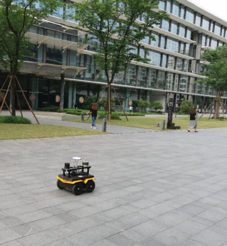
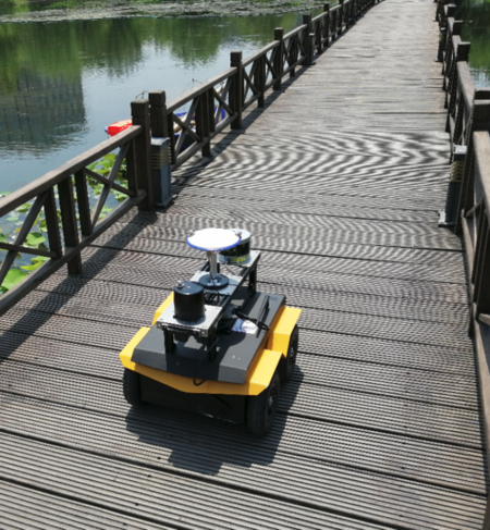
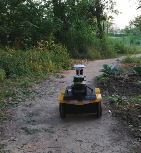
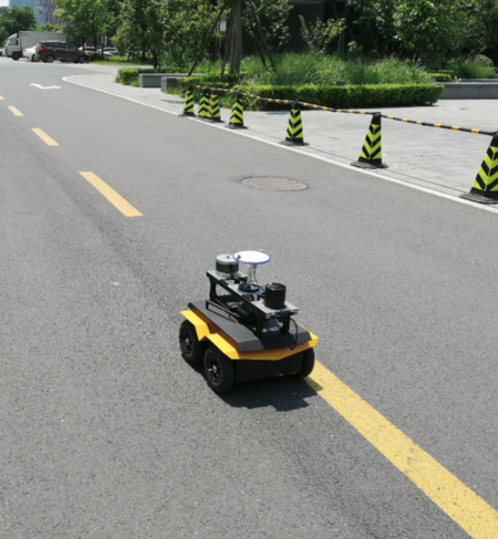
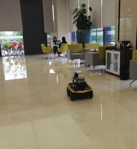
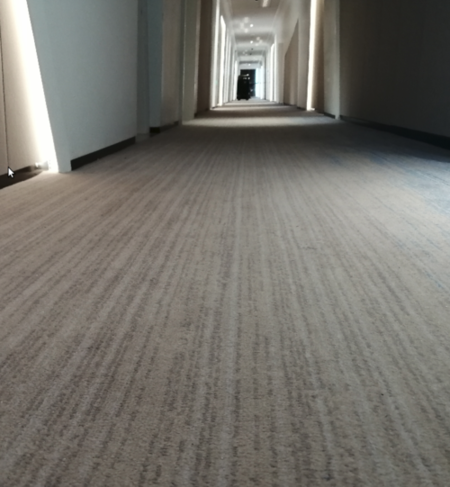
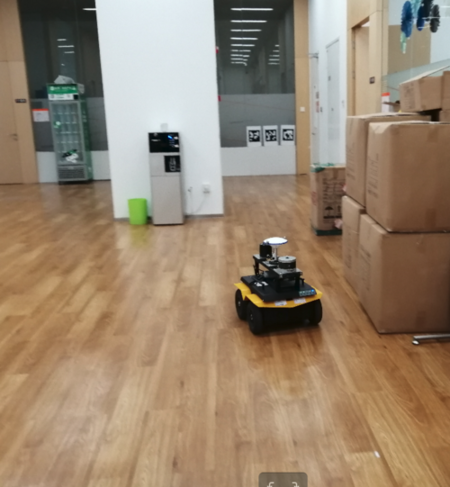
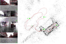
The first experiment is to demonstrate the improvement of localization accuracy by estimating (Eq. 2) online. As shown in Fig 3, we conducted experiments under different environments, i.e., (a) lawn, (b) cement brick, (c) wooden bridge, (d) muddy road, (e) asphalt road, (f) ceramic tiles, (g) carpet, and (h) wooden floor. Fig. 4 shows the trajectory and visual features estimated by the proposed method on sequence "CP01-2019-05-27-14-50-49", in which the robot traversed outdoors and indoors. Since GPS signal is not available in all tests (e.g., indoor tests), we here used final drift as the first error metric. To make this possible, we started and terminated each experiment at the same position. Two algorithms were implemented in this test: 1) the proposed one by explicitly estimating , and 2) using Eq. 3 without modeling 333In fact, Eq. 3 can be considered as one-parameter approximation of skid-steering kinematics, if is probabilistically estimated..
In Table. 1, we show the final drift values on 20 representative sequences. Since we used the two robots, we used the notation “CP01, CP02" to denote the names of the robots. Table. 1 clearly demonstrates that when skid-steering kinematic parameters are estimated online, the localization accuracy can be significantly improved. In fact, in almost half of the tests, the errors are reduced by approximately a order of magnitude. This validates our claim that to use odometer measurements of skid-steering robots, the complicated mechanism must be explicitly modeled to avoid accuracy loss.
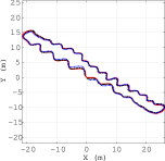
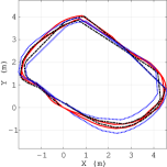
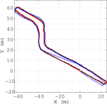
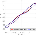
In some sequences where GPS signals were available, we also evaluated the positional root mean square errors (RMSE)[31]. To compute that, we interpolated the estimated poses to get the ones corresponding to the timestamp of GPS measurements. The RMSE errors are shown in Table. 2, which demonstrate that estimating is beneficial for trajectory tracking. Trajectory estimates on representative sequences are shown in Fig. 5.
| W/ | W/O | |||||||
| Sequence | Length(m) | Terrain | Norm(m) | x(m) | y(m) | Norm(m) | x(m) | y(m) |
| CP01-2019-04-19-15-42-40 | 632.64 | (b,f) | 0.82 | 0.74 | 0.37 | 9.41 | 6.14 | 7.12 |
| CP01-2019-04-19-15-56-09 | 629.96 | (b,f) | 1.87 | 1.06 | 1.54 | 9.94 | 6.16 | 7.80 |
| CP01-2019-04-19-16-09-53 | 626.83 | (b,f) | 1.56 | 1.28 | 0.89 | 8.35 | 5.70 | 6.10 |
| CP01-2019-05-08-18-06-43 | 51.44 | (a) | 0.09 | 0.07 | 0.06 | 0.22 | 0.14 | 0.17 |
| CP01-2019-05-08-17-50-51 | 204.81 | (e) | 0.23 | 0.17 | 0.15 | 0.44 | 0.25 | 0.36 |
| CP01-2019-05-08-17-42-01 | 436.19 | (e) | 0.57 | 0.46 | 0.33 | 1.81 | 0.99 | 1.51 |
| CP01-2019-04-19-14-57-38 | 372.15 | (b) | 1.62 | 1.18 | 1.12 | 4.93 | 3.69 | 3.26 |
| CP01-2019-05-27-14-32-36 | 110.55 | (b) | 0.37 | 0.30 | 0.22 | 0.39 | 0.16 | 0.36 |
6.1 Convergence of Kinematic Parameters
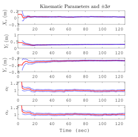
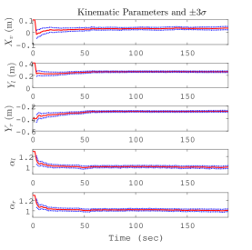
In this section, we show tests to demonstrate the convergence of under general motion. Unlike the experiments in the previous section where relatively good initial values of kinematic parameters were used, we manually set ‘bad’ initial value to kinematic parameters. Specifically, we added following error terms to initial kinematic parameters used in the previous section (good values): . We carried out tests on outdoor sequence "CP01-2019-05-08-17-50-51" and indoor sequence "CP01-2019-05-27-14-41-33", which did not involve changes of terrain types on the fly. In Fig. 6, the estimates of kinematic parameters are shown, along with the corresponding uncertainty envelopes.The results demonstrate that the kinematic parameters quickly converge to their correct values, and remains slow change rates for the rest of the trajectory. The uncertainty envelopes also shrink quickly. The results exactly meet our theoretical expectations that is locally identifiable under general motion.
7 Conclusions
In this paper, we have developed a novel kinematics-constrained visual-inertial localization method specialized for skid-steering robots, where a tightly-coupled sliding-window BA serves as the estimation engine for fusing multi-modal measurements. In particular, we have explicitly modeled the kinematics of skid-steering robots using both track ICRs and scale factors, in order to compensate for complex track-to-terrain interactions, imperfectness of mechanical design and terrain smoothness. Moreover, we have carefully examined the observability analysis, showing that the kinematic parameters are observable under general motion. Extensive real-world validations confirm that online kinematic estimation significantly improves localization.
References
- [1] “https://www.clearpathrobotics.com/jackal-small-unmanned-ground-vehicle/”
- [2] Mingyang Li and Anastasios I. Mourikis “High-precision, consistent EKF-based visual-inertial odometry” In The International Journal of Robotics Research 32.6, 2013, pp. 690–711
- [3] Mingyang Li, Hongsheng Yu, Xing Zheng and Anastasios I Mourikis “High-fidelity sensor modeling and self-calibration in vision-aided inertial navigation” In ICRA, 2014, pp. 409–416
- [4] Tong Qin, Peiliang Li and Shaojie Shen “VINS-mono: A robust and versatile monocular visual-inertial state estimator” In IEEE Transactions on Robotics 34.4, 2018, pp. 1004–1020
- [5] X. Zheng, Z. Moratto, M. Li and A. I. Mourikis “Photometric patch-based visual-inertial odometry” In IEEE International Conference on Robotics and Automation (ICRA), 2017, pp. 3264–3271
- [6] Kevin Eckenhoff, Patrick Geneva and Guoquan Huang “Closed-form Preintegration Methods for Graph-based Visual-Inertial Navigation” In International Journal of Robotics Research 38.5, 2019, pp. 563–586
- [7] R. Hartley, M. G. Jadidi, L. Gan, J. Huang, J. W. Grizzle and R. M. Eustice
- [8] Jorge L Martínez, Anthony Mandow, Jesús Morales, Salvador Pedraza and Alfonso García-Cerezo “Approximating kinematics for tracked mobile robots” In The International Journal of Robotics Research 24.10, 2005, pp. 867–878
- [9] Goran Huskic, Sebastian Buck and Andreas Zell “Path following control of skid-steered wheeled mobile robots at higher speeds on different terrain types” In IEEE International Conference on Robotics and Automation (ICRA), 2017, pp. 3734–3739
- [10] Jesse Pentzer, Sean Brennan and Karl Reichard “The use of unicycle robot control strategies for skid-steer robots through the ICR kinematic mapping” In IEEE/RSJ International Conference on Intelligent Robots and Systems, 2014, pp. 3201–3206
- [11] Jingang Yi, Hongpeng Wang, Junjie Zhang, Dezhen Song, Suhada Jayasuriya and Jingtai Liu “Kinematic modeling and analysis of skid-steered mobile robots with applications to low-cost inertial-measurement-unit-based motion estimation” In IEEE transactions on robotics 25.5, 2009
- [12] Cuifeng Wang, Wenjun Lv, Xiaochuan Li and Mingliang Mei “Terrain Adaptive Estimation of Instantaneous Centres of Rotation for Tracked Robots” In Complexity, 2018
- [13] Kejian J Wu, Chao X Guo, Georgios Georgiou and Stergios I Roumeliotis “VINS on wheels” In IEEE International Conference on Robotics and Automation, 2017, pp. 5155–5162
- [14] Mingyang Li and Anastasios I Mourikis “Online temporal calibration for camera–IMU systems: Theory and algorithms” In The International Journal of Robotics Research SAGE Publications Sage UK: London, England, 2014
- [15] Cesar Cadena, Luca Carlone, Henry Carrillo, Yasir Latif, Davide Scaramuzza, Jose Neira, Ian D. Reid and John J. Leonard “Past, Present, and Future of Simultaneous Localization and Mapping: Toward the Robust-Perception Age” In IEEE Transactions on Robotics 32.6, 2016, pp. 1309–1332
- [16] Andrea Censi, Antonio Franchi, Luca Marchionni and Giuseppe Oriolo “Simultaneous calibration of odometry and sensor parameters for mobile robots” In IEEE Transactions on Robotics 29.2 IEEE, 2013, pp. 475–492
- [17] Davide Scaramuzza “1-point-ransac structure from motion for vehicle-mounted cameras by exploiting non-holonomic constraints” In International journal of computer vision 95.1, 2011, pp. 74–85
- [18] Teddy Yap, Mingyang Li, Anastasios I Mourikis and Christian R Shelton “A particle filter for monocular vision-aided odometry” In IEEE International Conference on Robotics and Automation, 2011, pp. 5663–5669
- [19] Jorge L Martínez, Jesús Morales, Anthony Mandow, Salvador Pedraza and Alfonso García-Cerezo “Inertia-based ICR kinematic model for tracked skid-steer robots” In IEEE International Symposium on Safety, Security and Rescue Robotics (SSRR), 2017, pp. 166–171
- [20] Giulio Reina and Rocco Galati “Slip-based terrain estimation with a skid-steer vehicle” In Vehicle System Dynamics 54.10, 2016, pp. 1384–1404
- [21] Masataku Sutoh, Yutaro Iijima, Yuta Sakakieda and Sachiko Wakabayashi “Motion modeling and localization of skid-steering wheeled rover on loose terrain” In IEEE Robotics and Automation Letters 3.4, 2018, pp. 4031–4037
- [22] Wenjun Lv, Yu Kang and Jiahu Qin “FVO: floor vision aided odometry” In Science China Information Sciences 62.1, 2019, pp. 12202
- [23] Wenjun Lv, Yu Kang and Jiahu Qin “Indoor localization for skid-steering mobile robot by fusing encoder, gyroscope, and magnetometer” In IEEE Transactions on Systems, Man, and Cybernetics: Systems, 2017, pp. 1–13
- [24] Jesse Pentzer, Sean Brennan and Karl Reichard “Model-based Prediction of Skid-steer Robot Kinematics Using Online Estimation of Track Instantaneous Centers of Rotation” In Journal of Field Robotics 31.3, 2014, pp. 455–476
- [25] Meixiang Quan, Songhao Piao, Minglang Tan and Shi-Sheng Huang “Tightly-coupled Monocular Visual-odometric SLAM using Wheels and a MEMS Gyroscope” In arXiv:1804.04854, 2018
- [26] Stefan Leutenegger, Simon Lynen, Michael Bosse, Roland Siegwart and Paul Furgale “Keyframe-based visual–inertial odometry using nonlinear optimization” In The International Journal of Robotics Research 34.3 SAGE Publications Sage UK: London, England, 2015, pp. 314–334
- [27] Edward Rosten and Tom Drummond “Machine learning for high-speed corner detection” In European conference on computer vision, 2006, pp. 430–443 Springer
- [28] Bruce D Lucas and Takeo Kanade “An iterative image registration technique with an application to stereo vision” Vancouver, British Columbia, 1981
- [29] Xingxing Zuo, Guoquan Huang and Mingyang Li “Visual Localization for Skid-Steering Robots” Available: http://udel.edu/~ghuang/papers/tr_icr.pdf, 2019
- [30] Mingming Zhang, Yiming Chen and Mingyang Li “Vision-Aided Localization For Ground Vehicle” In IEEE/RSJ International Conference on Intelligent Robots and Systems, 2019
- [31] Y. Bar-Shalom and T. E. Fortmann “Tracking and Data Association” New York: Academic Press, 1988
- [32] Richard Hartley and Andrew Zisserman “Multiple view geometry in computer vision” Cambridge university press, 2003
- [33] Jorn FM Van Doren, Sippe G Douma, Paul MJ Hof, Jan Dirk Jansen and Okko H Bosgra “Identifiability: from qualitative analysis to model structure approximation” In IFAC Proceedings Volumes 42.10 Elsevier, 2009, pp. 664–669