Constant Curvature Graph Convolutional Networks

Gregor Bachmann    Gary Bécigneul    Octavian-Eugen Ganea
Abstract

Interest has been rising lately towards methods representing data in non-Euclidean spaces, e.g. hyperbolic or spherical, that provide specific inductive biases useful for certain real-world data properties, e.g. scale-free, hierarchical or cyclical. However, the popular graph neural networks are currently limited in modeling data only via Euclidean geometry and associated vector space operations. Here, we bridge this gap by proposing mathematically grounded generalizations of graph convolutional networks (GCN) to (products of) constant curvature spaces. We do this by i) introducing a unified formalism that can interpolate smoothly between all geometries of constant curvature, ii) leveraging gyro-barycentric coordinates that generalize the classic Euclidean concept of the center of mass. Our class of models smoothly recover their Euclidean counterparts when the curvature goes to zero from either side. Empirically, we outperform Euclidean GCNs in the tasks of node classification and distortion minimization for symbolic data exhibiting non-Euclidean behavior, according to their discrete curvature.

Machine Learning, ICML, hyperbolic, hierarchical, curvature, manifold, geometry, graph, neural, convolutional, network, message passing, representation, spherical, aggregation, midpoint, gyro, euclidean

1 Introduction

Refer to caption
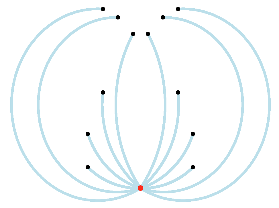
Figure 1: Euclidean embeddings of trees of different depths. All the four most inner circles are identical. Ideal node embeddings should match in distance the graph metric, e.g. the distance between the pink and green nodes should be the same as their shortest path length. Notice how we quickly run out of space, e.g. the pink and green nodes get closer as opposed to farther. This issue is resolved when embedding trees in hyperbolic spaces.
Graph Convolutional Networks.

The success of convolutional networks and deep learning for image data has inspired generalizations for graphs for which sharing parameters is consistent with the graph geometry. Bruna et al. (2014); Henaff et al. (2015) are the pioneers of spectral graph convolutional neural networks in the graph Fourier space using localized spectral filters on graphs. However, in order to reduce the graph-dependency on the Laplacian eigenmodes, Defferrard et al. (2016) approximate the convolutional filters using Chebyshev polynomials leveraging a result of Hammond et al. (2011). The resulting method (discussed in Appendix A) is computationally efficient and superior in terms of accuracy and complexity. Further, Kipf & Welling (2017) simplify this approach by considering first-order approximations obtaining high scalability. The proposed graph convolutional networks (GCN) is interpolating node embeddings via a symmetrically normalized adjacency matrix, while this weight sharing can be understood as an efficient diffusion-like regularizer. Recent works extend GCNs to achieve state of the art results for link prediction (Zhang & Chen, 2018), graph classification (Hamilton et al., 2017; Xu et al., 2018) and node classification (Klicpera et al., 2019; Veličković et al., 2018).

Euclidean geometry in ML.

In machine learning (ML), data is most often represented in a Euclidean space for various reasons. First, some data is intrinsically Euclidean, such as positions in 3D space in classical mechanics. Second, intuition is easier in such spaces, as they possess an appealing vectorial structure allowing basic arithmetic and a rich theory of linear algebra. Finally, a lot of quantities of interest such as distances and inner-products are known in closed-form formulae and can be computed very efficiently on the existing hardware. These operations are the basic building blocks for most of today’s popular machine learning models. Thus, the powerful simplicity and efficiency of Euclidean geometry has led to numerous methods achieving state-of-the-art on tasks as diverse as machine translation (Bahdanau et al., 2015; Vaswani et al., 2017), speech recognition (Graves et al., 2013), image classification (He et al., 2016) or recommender systems (He et al., 2017).

Riemannian ML.

In spite of this success, certain types of data (e.g. hierarchical, scale-free or spherical data) have been shown to be better represented by non-Euclidean geometries (Defferrard et al., 2019; Bronstein et al., 2017; Nickel & Kiela, 2017; Gu et al., 2019), leading in particular to the rich theories of manifold learning (Roweis & Saul, 2000; Tenenbaum et al., 2000) and information geometry (Amari & Nagaoka, 2007). The mathematical framework in vigor to manipulate non-Euclidean geometries is known as Riemannian geometry (Spivak, 1979). Although its theory leads to many strong and elegant results, some of its basic quantities such as the distance function d(,)𝑑d(\cdot,\cdot) are in general not available in closed-form, which can be prohibitive to many computational methods.

Representational Advantages of Geometries of Constant Curvature.

An interesting trade-off between general Riemannian manifolds and the Euclidean space is given by manifolds of constant sectional curvature. They define together what are called hyperbolic (negative curvature), elliptic (positive curvature) and Euclidean (zero curvature) geometries. As discussed below and in Appendix B, Euclidean spaces have limitations and suffer from large distortion when embedding certain types of data such as trees. In these cases, the hyperbolic and spherical spaces have representational advantages providing a better inductive bias for the respective data.

The hyperbolic space can be intuitively understood as a continuous tree: the volume of a ball grows exponentially with its radius, similarly as how the number of nodes in a binary tree grows exponentially with its depth (see fig. 1). Its tree-likeness properties have long been studied mathematically (Gromov, 1987; Hamann, 2017; Ungar, 2008) and it was proven to better embed complex networks (Krioukov et al., 2010), scale-free graphs and hierarchical data compared to the Euclidean geometry (Cho et al., 2019; Sala et al., 2018; Ganea et al., 2018b; Gu et al., 2019; Nickel & Kiela, 2018, 2017; Tifrea et al., 2019). Several important tools or methods found their hyperbolic counterparts, such as variational autoencoders (Mathieu et al., 2019; Ovinnikov, 2019), attention mechanisms (Gulcehre et al., 2018), matrix multiplications, recurrent units and multinomial logistic regression (Ganea et al., 2018a).

Similarly, spherical geometry provides benefits for modeling spherical or cyclical data (Defferrard et al., 2019; Matousek, 2013; Davidson et al., 2018; Xu & Durrett, 2018; Gu et al., 2019; Grattarola et al., 2018; Wilson et al., 2014).

Computational Efficiency of Constant Curvature Spaces (CCS).

CCS are some of the few Riemannian manifolds to possess closed-form formulae for geometric quantities of interest in computational methods, i.e. distance, geodesics, exponential map, parallel transport and their gradients. We also leverage here the closed expressions for weighted centroids.

“Linear Algebra” of CCS: Gyrovector Spaces.

In order to study the geometry of constant negative curvature in analogy with the Euclidean geometry, Ungar (1999, 2005, 2008, 2016) proposed the elegant non-associative algebraic formalism of gyrovector spaces. Recently, Ganea et al. (2018a) have linked this framework to the Riemannian geometry of the space, also generalizing the building blocks for non-Euclidean deep learning models operating with hyperbolic data representations.

However, it remains unclear how to extend in a principled manner the connection between Riemannian geometry and gyrovector space operations for spaces of constant positive curvature (spherical). By leveraging Euler’s formula and complex analysis, we present to our knowledge the first unified gyro framework that allows for a differentiable interpolation between geometries of constant curvatures irrespective of their signs. This is possible when working with the Poincaré ball and stereographic spherical projection models of respectively hyperbolic and spherical spaces.

GCNs in Constant Curvature Spaces.

In this work, we introduce an extension of graph convolutional networks that allows to learn representations residing in (products of) constant curvature spaces with any curvature sign. We achieve this by combining the derived unified gyro framework together with the effectiveness of GCNs (Kipf & Welling, 2017). Concurrent to our work, Chami et al. (2019); Liu et al. (2019) consider graph neural networks that learn embeddings in hyperbolic space via tangent space aggregation. Their approach will be analyzed more closely in section 3.4. Our model is more general as it produces representations in a strict super-set containing the hyperbolic space.

2 The Geometry of Constant Curvature Spaces

Riemannian Geometry.

A manifold \mathcal{M} of dimension d𝑑d is a generalization to higher dimensions of the notion of surface, and is a space that locally looks like dsuperscript𝑑\mathbb{R}^{d}. At each point 𝐱𝐱{\mathbf{x}}\in\mathcal{M}, \mathcal{M} can be associated a tangent space T𝐱subscript𝑇𝐱T_{\mathbf{x}}\mathcal{M}, which is a vector space of dimension d𝑑d that can be understood as a first order approximation of \mathcal{M} around 𝐱𝐱{\mathbf{x}}. A Riemannian metric g𝑔g is given by an inner-product g𝐱(,)subscript𝑔𝐱g_{\mathbf{x}}(\cdot,\cdot) at each tangent space T𝐱subscript𝑇𝐱T_{\mathbf{x}}\mathcal{M}, g𝐱subscript𝑔𝐱g_{\mathbf{x}} varying smoothly with 𝐱𝐱{\mathbf{x}}. A given g𝑔g defines the geometry of \mathcal{M}, because it can be used to define the distance between 𝐱𝐱{\mathbf{x}} and 𝐲𝐲{\mathbf{y}} as the infimum of the lengths of smooth paths γ:[0,1]:𝛾01\gamma:[0,1]\to\mathcal{M} from 𝐱𝐱{\mathbf{x}} to 𝐲𝐲{\mathbf{y}}, where the length is defined as (γ):=01gγ(t)(γ˙(t),γ˙(t))dtassign𝛾superscriptsubscript01subscript𝑔𝛾𝑡˙𝛾𝑡˙𝛾𝑡differential-d𝑡\ell(\gamma):=\int_{0}^{1}\sqrt{g_{\gamma(t)}(\dot{\gamma}(t),\dot{\gamma}(t))}\mathrm{d}t . Under certain assumptions, a given g𝑔g also defines a curvature at each point.
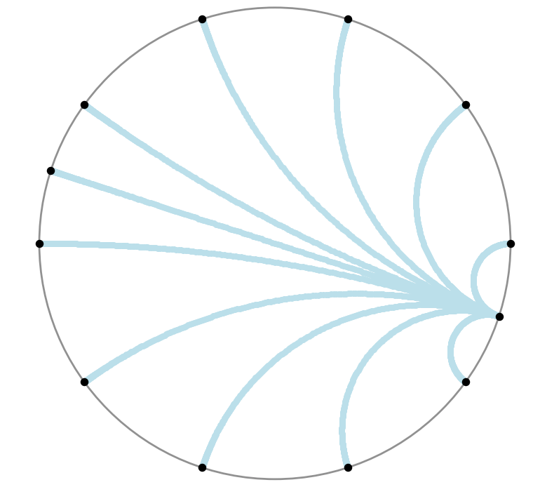
Refer to caption
Refer to caption
Figure 2: Geodesics in the Poincaré disk (left) and the stereographic projection of the sphere (right).
Unifying all curvatures κ𝜅\kappa.

There exist several models of respectively constant positive and negative curvatures. For positive curvature, we choose the stereographic projection of the sphere, while for negative curvature we choose the Poincaré model which is the stereographic projection of the Lorentz model. As explained below, this choice allows us to generalize the gyrovector space framework and unify spaces of both positive and negative curvature κ𝜅\kappa into a single model which we call the κ𝜅\kappa-stereographic model.

Refer to caption
Refer to caption
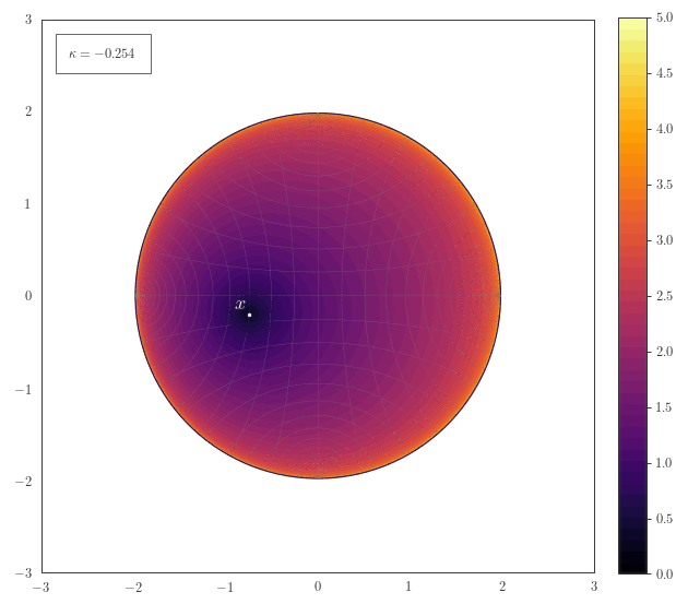
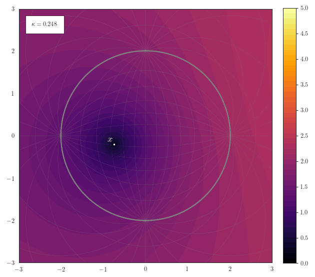
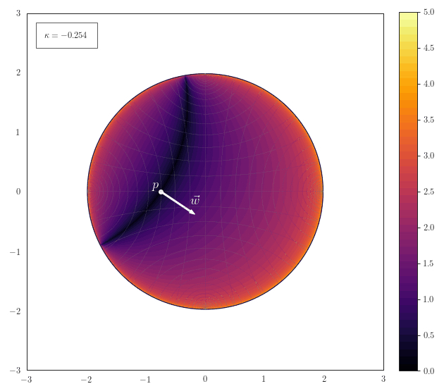
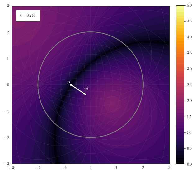
Figure 3: Heatmap of the distance function dκ(𝐱,)subscript𝑑𝜅𝐱d_{\kappa}({\mathbf{x}},\cdot) in 𝔰𝔱κ2𝔰subscriptsuperscript𝔱2𝜅\mathfrak{st}^{2}_{\kappa} for κ=0.254𝜅0.254\kappa=-0.254 (left) and κ=0.248𝜅0.248\kappa=0.248 (right).
The κ𝜅\kappa-stereographic model.

For a curvature κ𝜅\kappa\in\mathbb{R} and a dimension d2𝑑2d\geq 2, we study the model 𝔰𝔱κd𝔰subscriptsuperscript𝔱𝑑𝜅\mathfrak{st}^{d}_{\kappa} defined as 𝔰𝔱κd={𝐱dκ𝐱22<1}𝔰subscriptsuperscript𝔱𝑑𝜅conditional-set𝐱superscript𝑑𝜅superscriptsubscriptnorm𝐱221\mathfrak{st}^{d}_{\kappa}=\{{\mathbf{x}}\in\mathbb{R}^{d}\mid-\kappa\|{\mathbf{x}}\|_{2}^{2}<1\} equipped with its Riemannian metric g𝐱κ=4(1+κ𝐱2)2𝐈=:(λ𝐱κ)2𝐈g_{{\mathbf{x}}}^{\kappa}=\frac{4}{(1+\kappa||{\mathbf{x}}||^{2})^{2}}{\mathbf{I}}=:(\lambda_{{\mathbf{x}}}^{\kappa})^{2}{\mathbf{I}}. Note in particular that when κ0𝜅0\kappa\geq 0, 𝔰𝔱κd𝔰subscriptsuperscript𝔱𝑑𝜅\mathfrak{st}^{d}_{\kappa} is dsuperscript𝑑\mathbb{R}^{d}, while when κ<0𝜅0\kappa<0 it is the open ball of radius 1/κ1𝜅1/\sqrt{-\kappa}.

Gyrovector spaces & Riemannian geometry.

As discussed in section 1, the gyrovector space formalism is used to generalize vector spaces to the Poincaré model of hyperbolic geometry (Ungar, 2005, 2008). In addition, important quantities from Riemannian geometry can be rewritten in terms of the Möbius vector addition and scalar-vector multiplication (Ganea et al., 2018a). We here extend gyrovector spaces to the κ𝜅\kappa-stereographic model, i.e. allowing positive curvature.

For κ>0𝜅0\kappa>0 and any point 𝐱𝔰𝔱κd𝐱𝔰superscriptsubscript𝔱𝜅𝑑{\mathbf{x}}\in\mathfrak{st}_{\kappa}^{d}, we will denote by 𝐱~~𝐱\tilde{{\mathbf{x}}} the unique point of the sphere of radius κ12superscript𝜅12\kappa^{-\frac{1}{2}} in d+1superscript𝑑1\mathbb{R}^{d+1} whose stereographic projection is 𝐱𝐱{\mathbf{x}}. As detailed in Appendix C, it is given by

𝐱~:=(λ𝐱κ𝐱,κ12(λ𝐱κ1)).assign~𝐱subscriptsuperscript𝜆𝜅𝐱𝐱superscript𝜅12superscriptsubscript𝜆𝐱𝜅1\tilde{{\mathbf{x}}}:=(\lambda^{\kappa}_{\mathbf{x}}{\mathbf{x}},\kappa^{-\frac{1}{2}}(\lambda_{\mathbf{x}}^{\kappa}-1)). (1)

For 𝐱,𝐲𝔰𝔱κd𝐱𝐲𝔰subscriptsuperscript𝔱𝑑𝜅{\mathbf{x}},{\mathbf{y}}\in\mathfrak{st}^{d}_{\kappa}, we define the κ𝜅\kappa-addition, in the κ𝜅\kappa-stereographic model by:

𝐱κ𝐲=(12κ𝐱T𝐲κ𝐲2)𝐱+(1+κ𝐱2)𝐲12κ𝐱T𝐲+κ2𝐱2𝐲2𝔰𝔱κd.subscriptdirect-sum𝜅𝐱𝐲12𝜅superscript𝐱𝑇𝐲𝜅superscriptnorm𝐲2𝐱1𝜅superscriptnorm𝐱2𝐲12𝜅superscript𝐱𝑇𝐲superscript𝜅2superscriptnorm𝐱2superscriptnorm𝐲2𝔰superscriptsubscript𝔱𝜅𝑑{\mathbf{x}}\oplus_{\kappa}{\mathbf{y}}=\frac{(1-2\kappa{\mathbf{x}}^{T}{\mathbf{y}}-\kappa||{\mathbf{y}}||^{2}){\mathbf{x}}+(1+\kappa||{\mathbf{x}}||^{2}){\mathbf{y}}}{1-2\kappa{\mathbf{x}}^{T}{\mathbf{y}}+\kappa^{2}||{\mathbf{x}}||^{2}||{\mathbf{y}}||^{2}}\in\mathfrak{st}_{\kappa}^{d}. (2)

The κ𝜅\kappa-addition is defined in all the cases except for spherical geometry and 𝐱=𝐲/(κ𝐲2)𝐱𝐲𝜅superscriptnorm𝐲2{\mathbf{x}}={\mathbf{y}}/(\kappa\|{\mathbf{y}}\|^{2}) as stated by the following theorem proved in Appendix C.2.1.

Theorem 1 (Definiteness of κ𝜅\kappa-addition).
We have
12κ𝐱T𝐲+κ2𝐱2𝐲2=012𝜅superscript𝐱𝑇𝐲superscript𝜅2superscriptnorm𝐱2superscriptnorm𝐲201-2\kappa{\mathbf{x}}^{T}{\mathbf{y}}+\kappa^{2}||{\mathbf{x}}||^{2}||{\mathbf{y}}||^{2}=0 if and only if κ>0𝜅0\kappa>0 and 𝐱=𝐲/(κ𝐲2)𝐱𝐲𝜅superscriptnorm𝐲2{\mathbf{x}}={\mathbf{y}}/(\kappa\|{\mathbf{y}}\|^{2}).

For s𝑠s\in\mathbb{R} and 𝐱𝔰𝔱κd𝐱𝔰superscriptsubscript𝔱𝜅𝑑{\mathbf{x}}\in\mathfrak{st}_{\kappa}^{d} (and |stanκ1𝐱|<κ12π/2𝑠superscriptsubscript𝜅1norm𝐱superscript𝜅12𝜋2|s\tan_{\kappa}^{-1}\|{\mathbf{x}}\||<\kappa^{\frac{1}{2}}\pi/2 if κ>0𝜅0\kappa>0), the κ𝜅\kappa-scaling in the κ𝜅\kappa-stereographic model is given by:

sκ𝐱=tanκ(stanκ1𝐱)𝐱𝐱𝔰𝔱κd,subscripttensor-product𝜅𝑠𝐱subscript𝜅𝑠superscriptsubscript𝜅1norm𝐱𝐱norm𝐱𝔰subscriptsuperscript𝔱𝑑𝜅s\otimes_{\kappa}{\mathbf{x}}=\tan_{\kappa}{(s\cdot\tan_{\kappa}^{-1}||{\mathbf{x}}||)}\frac{{\mathbf{x}}}{||{\mathbf{x}}||}\in\mathfrak{st}^{d}_{\kappa}, (3)

where tanκsubscript𝜅\tan_{\kappa} equals κ1/2tansuperscript𝜅12\kappa^{-1/2}\tan if κ>0𝜅0\kappa>0 and (κ)1/2tanhsuperscript𝜅12(-\kappa)^{-1/2}\tanh if κ<0𝜅0\kappa<0. This formalism yields simple closed-forms for various quantities including the distance function (see fig. 3) inherited from the Riemannian manifold (𝔰𝔱κd𝔰superscriptsubscript𝔱𝜅𝑑\mathfrak{st}_{\kappa}^{d}, gκsuperscript𝑔𝜅g^{\kappa}), the exp and log maps, and geodesics (see fig. 2), as shown by the following theorem.

Theorem 2 (Extending gyrovector spaces to positive curvature).
For 𝐱,𝐲𝔰𝔱κd𝐱𝐲𝔰subscriptsuperscript𝔱𝑑𝜅{\mathbf{x}},{\mathbf{y}}\in\mathfrak{st}^{d}_{\kappa}, 𝐱𝐲𝐱𝐲{\mathbf{x}}\neq{\mathbf{y}}, 𝐯𝟎𝐯0\mathbf{v}\neq\mathbf{0}, (and 𝐱𝐲/(κ𝐲2)𝐱𝐲𝜅superscriptnorm𝐲2{\mathbf{x}}\neq-{\mathbf{y}}/(\kappa\|{\mathbf{y}}\|^{2}) if κ>0𝜅0\kappa>0), the distance function is given by111We write 𝐱𝐲direct-sum𝐱𝐲-{\mathbf{x}}\oplus{\mathbf{y}} for (𝐱)𝐲direct-sum𝐱𝐲(-{\mathbf{x}})\oplus{\mathbf{y}} and not (𝐱𝐲)direct-sum𝐱𝐲-({\mathbf{x}}\oplus{\mathbf{y}}).: dκ(𝐱,𝐲)=2|κ|1/2tanκ1𝐱κ𝐲,subscript𝑑𝜅𝐱𝐲2superscript𝜅12superscriptsubscript𝜅1normsubscriptdirect-sum𝜅𝐱𝐲d_{\kappa}({\mathbf{x}},{\mathbf{y}})=2|\kappa|^{-1/2}\tan_{\kappa}^{-1}\|-{\mathbf{x}}\oplus_{\kappa}{\mathbf{y}}\|, (4) the unit-speed geodesic from 𝐱𝐱{\mathbf{x}} to 𝐲𝐲{\mathbf{y}} is unique and given by γ𝐱𝐲(t)=𝐱κ(tκ(𝐱κ𝐲)),subscript𝛾𝐱𝐲𝑡subscriptdirect-sum𝜅𝐱subscripttensor-product𝜅𝑡subscriptdirect-sum𝜅𝐱𝐲\gamma_{{\mathbf{x}}\to{\mathbf{y}}}(t)={\mathbf{x}}\oplus_{\kappa}\left(t\otimes_{\kappa}(-{\mathbf{x}}\oplus_{\kappa}{\mathbf{y}})\right), (5) and finally the exponential and logarithmic maps are described as: exp𝐱κ(𝐯)superscriptsubscript𝐱𝜅𝐯\displaystyle\exp_{{\mathbf{x}}}^{\kappa}({\mathbf{v}}) =𝐱κ(tanκ(|κ|12λ𝐱κ𝐯2)𝐯𝐯)absentsubscriptdirect-sum𝜅𝐱subscript𝜅superscript𝜅12superscriptsubscript𝜆𝐱𝜅norm𝐯2𝐯norm𝐯\displaystyle={\mathbf{x}}\oplus_{\kappa}\left(\tan_{\kappa}\left(|\kappa|^{\frac{1}{2}}\frac{\lambda_{{\mathbf{x}}}^{\kappa}||\mathbf{v}||}{2}\right)\frac{\mathbf{v}}{||{\mathbf{v}}||}\right) (6) log𝐱κ(𝐲)superscriptsubscript𝐱𝜅𝐲\displaystyle\log_{{\mathbf{x}}}^{\kappa}({\mathbf{y}}) =2|κ|12λ𝐱κtanκ1𝐱κ𝐲𝐱κ𝐲𝐱k𝐲absent2superscript𝜅12superscriptsubscript𝜆𝐱𝜅superscriptsubscript𝜅1normsubscriptdirect-sum𝜅𝐱𝐲subscriptdirect-sum𝜅𝐱𝐲normsubscriptdirect-sum𝑘𝐱𝐲\displaystyle=\frac{2|\kappa|^{-\frac{1}{2}}}{\lambda_{{\mathbf{x}}}^{\kappa}}\tan_{\kappa}^{-1}||-{\mathbf{x}}\oplus_{\kappa}{\mathbf{y}}||\frac{-{\mathbf{x}}\oplus_{\kappa}{\mathbf{y}}}{||-{\mathbf{x}}\oplus_{k}{\mathbf{y}}||} (7)

Proof sketch:
The case κ0𝜅0\kappa\leq 0 was already taken care of by Ganea et al. (2018a). For κ>0𝜅0\kappa>0, we provide a detailed proof in Appendix C.2.2. The exponential map and unit-speed geodesics are obtained using the Egregium theorem and the known formulas in the standard spherical model. The distance then follows from the formula dκ(𝐱,𝐲)=log𝐱κ(𝐲)𝐱subscript𝑑𝜅𝐱𝐲subscriptnormsuperscriptsubscript𝐱𝜅𝐲𝐱d_{\kappa}({\mathbf{x}},{\mathbf{y}})=\|\log_{\mathbf{x}}^{\kappa}({\mathbf{y}})\|_{\mathbf{x}} which holds in any Riemannian manifold.

\square

Around κ=0𝜅0\kappa=0.

One notably observes that choosing κ=0𝜅0\kappa=0 yields all corresponding Euclidean quantities, which guarantees a continuous interpolation between κ𝜅\kappa-stereographic models of different curvatures, via Euler’s formula tan(x)=itanh(ix)𝑥𝑖𝑖𝑥\tan(x)=-i\tanh(ix) where i:=1assign𝑖1i:=\sqrt{-1}. But is this interpolation differentiable with respect to κ𝜅\kappa? It is, as shown by the following theorem, proved in Appendix C.2.3.

Theorem 3 (Differentiability of 𝔰𝔱κd𝔰subscriptsuperscript𝔱𝑑𝜅\mathfrak{st}^{d}_{\kappa} w.r.t. κ𝜅\kappa around 00).
Let 𝐯𝟎𝐯0\mathbf{v}\neq\mathbf{0} and 𝐱,𝐲d𝐱𝐲superscript𝑑{\mathbf{x}},{\mathbf{y}}\in\mathbb{R}^{d}, such that 𝐱𝐲𝐱𝐲{\mathbf{x}}\neq{\mathbf{y}} (and 𝐱𝐲/(κ𝐲2)𝐱𝐲𝜅superscriptnorm𝐲2{\mathbf{x}}\neq-{\mathbf{y}}/(\kappa\|{\mathbf{y}}\|^{2}) if κ>0𝜅0\kappa>0). Quantities in Eqs. (4,5,6, 7) are well-defined for |κ|<1/min(𝐱2,𝐲2)𝜅1superscriptnorm𝐱2superscriptnorm𝐲2|\kappa|<1/\min(\|{\mathbf{x}}\|^{2},\|{\mathbf{y}}\|^{2}), i.e. for κ𝜅\kappa small enough. Their first order derivatives at 0superscript00^{-} and 0+superscript00^{+} exist and are equal. Moreover, for the distance we have up to quadratic terms in κ𝜅\kappa: dκ(𝐱,𝐲)2𝐱𝐲2κ(𝐱𝐲3/3+(𝐱T𝐲)𝐱𝐲2)subscript𝑑𝜅𝐱𝐲2delimited-∥∥𝐱𝐲2𝜅superscriptdelimited-∥∥𝐱𝐲33superscript𝐱𝑇𝐲superscriptdelimited-∥∥𝐱𝐲2\begin{split}d_{\kappa}({\mathbf{x}},{\mathbf{y}})\approx{}&2\|{\mathbf{x}}-{\mathbf{y}}\|\\ &-2\kappa\Big{(}\|{\mathbf{x}}-{\mathbf{y}}\|^{3}/3+({\mathbf{x}}^{T}{\mathbf{y}})\|{\mathbf{x}}-{\mathbf{y}}\|^{2}\Big{)}\end{split} (8)

Note that for 𝐱T𝐲0superscript𝐱𝑇𝐲0{\mathbf{x}}^{T}{\mathbf{y}}\geq 0, this tells us that an infinitesimal change of curvature from zero to small negative, i.e. towards 0superscript00^{-}, while keeping 𝐱,𝐲𝐱𝐲{\mathbf{x}},{\mathbf{y}} fixed, has the effect of increasing their distance.

As a consequence, we have a unified formalism that allows for a differentiable interpolation between all three geometries of constant curvature.

3 κ𝜅\kappa-GCNs

We start by introducing the methods upon which we build. We present our models for spaces of constant sectional curvature, in the κ𝜅\kappa-stereographic model. However, the generalization to cartesian products of such spaces (Gu et al., 2019) follows naturally from these tools.

3.1 Graph Convolutional Networks

The problem of node classification on a graph has long been tackled with explicit regularization using the graph Laplacian (Weston et al., 2012). Namely, for a directed graph with adjacency matrix 𝐀𝐀{\mathbf{A}}, by adding the following term to the loss: i,j𝐀ijf(𝐱i)f(𝐱j)2=f(𝐗)T𝐋f(𝐗)subscript𝑖𝑗subscript𝐀𝑖𝑗superscriptnorm𝑓subscript𝐱𝑖𝑓subscript𝐱𝑗2𝑓superscript𝐗𝑇𝐋𝑓𝐗\sum_{i,j}{\mathbf{A}}_{ij}\|f({\mathbf{x}}_{i})-f({\mathbf{x}}_{j})\|^{2}=f({\mathbf{X}})^{T}{\mathbf{L}}f({\mathbf{X}}), where 𝐋=𝐃𝐀𝐋𝐃𝐀{\mathbf{L}}={\mathbf{D}}-{\mathbf{A}} is the (unnormalized) graph Laplacian, Dii:=kAikassignsubscript𝐷𝑖𝑖subscript𝑘subscript𝐴𝑖𝑘D_{ii}:=\sum_{k}A_{ik} defines the (diagonal) degree matrix, f𝑓f contains the trainable parameters of the model and 𝐗=(xij)ij𝐗subscriptsuperscriptsubscript𝑥𝑖𝑗𝑖𝑗{\mathbf{X}}=(x_{i}^{j})_{ij} the node features of the model. Such a regularization is expected to improve generalization if connected nodes in the graph tend to share labels; node i𝑖i with feature vector 𝐱isubscript𝐱𝑖{\mathbf{x}}_{i} is represented as f(𝐱i)𝑓subscript𝐱𝑖f({\mathbf{x}}_{i}) in a Euclidean space.

With the aim to obtain more scalable models, Defferrard et al. (2016); Kipf & Welling (2017) propose to make this regularization implicit by incorporating it into what they call graph convolutional networks (GCN), which they motivate as a first order approximation of spectral graph convolutions, yielding the following scalable layer architecture (detailed in Appendix A):

𝐇(t+1)=σ(𝐃~12𝐀~𝐃~12𝐇(t)𝐖(t))superscript𝐇𝑡1𝜎superscript~𝐃12~𝐀superscript~𝐃12superscript𝐇𝑡superscript𝐖𝑡{\mathbf{H}}^{(t+1)}=\sigma\left(\tilde{{\mathbf{D}}}^{-\frac{1}{2}}\tilde{{\mathbf{A}}}\tilde{{\mathbf{D}}}^{-\frac{1}{2}}{\mathbf{H}}^{(t)}{\mathbf{W}}^{(t)}\right) (9)

where 𝐀~=𝐀+𝐈~𝐀𝐀𝐈\tilde{{\mathbf{A}}}={\mathbf{A}}+{\mathbf{I}} has added self-connections, D~ii=kA~iksubscript~𝐷𝑖𝑖subscript𝑘subscript~𝐴𝑖𝑘\tilde{D}_{ii}=\sum_{k}\tilde{A}_{ik} defines its diagonal degree matrix, σ𝜎\sigma is a non-linearity such as sigmoid, tanh\tanh or ReLU=max(0,)ReLU0\mathrm{ReLU}=\max(0,\cdot), and 𝐖(t)superscript𝐖𝑡{\mathbf{W}}^{(t)} and 𝐇(t)superscript𝐇𝑡{\mathbf{H}}^{(t)} are the parameter and activation matrices of layer t𝑡t respectively, with 𝐇(0)=𝐗superscript𝐇0𝐗{\mathbf{H}}^{(0)}={\mathbf{X}} the input feature matrix.

3.2 Tools for a κ𝜅\kappa-GCN

Learning a parametrized function fθsubscript𝑓𝜃f_{\theta} that respects hyperbolic geometry has been studied in Ganea et al. (2018a): neural layers and hyperbolic softmax. We generalize their definitions into the κ𝜅\kappa-stereographic model, unifying operations in positive and negative curvature. We explain how curvature introduces a fundamental difference between left and right matrix multiplications, depicting the Möbius matrix multiplication of Ganea et al. (2018a) as a right multiplication, independent for each embedding. We then introduce a left multiplication by extension of gyromidpoints which ties the embeddings, which is essential for graph neural networks.
Refer to caption
Refer to caption
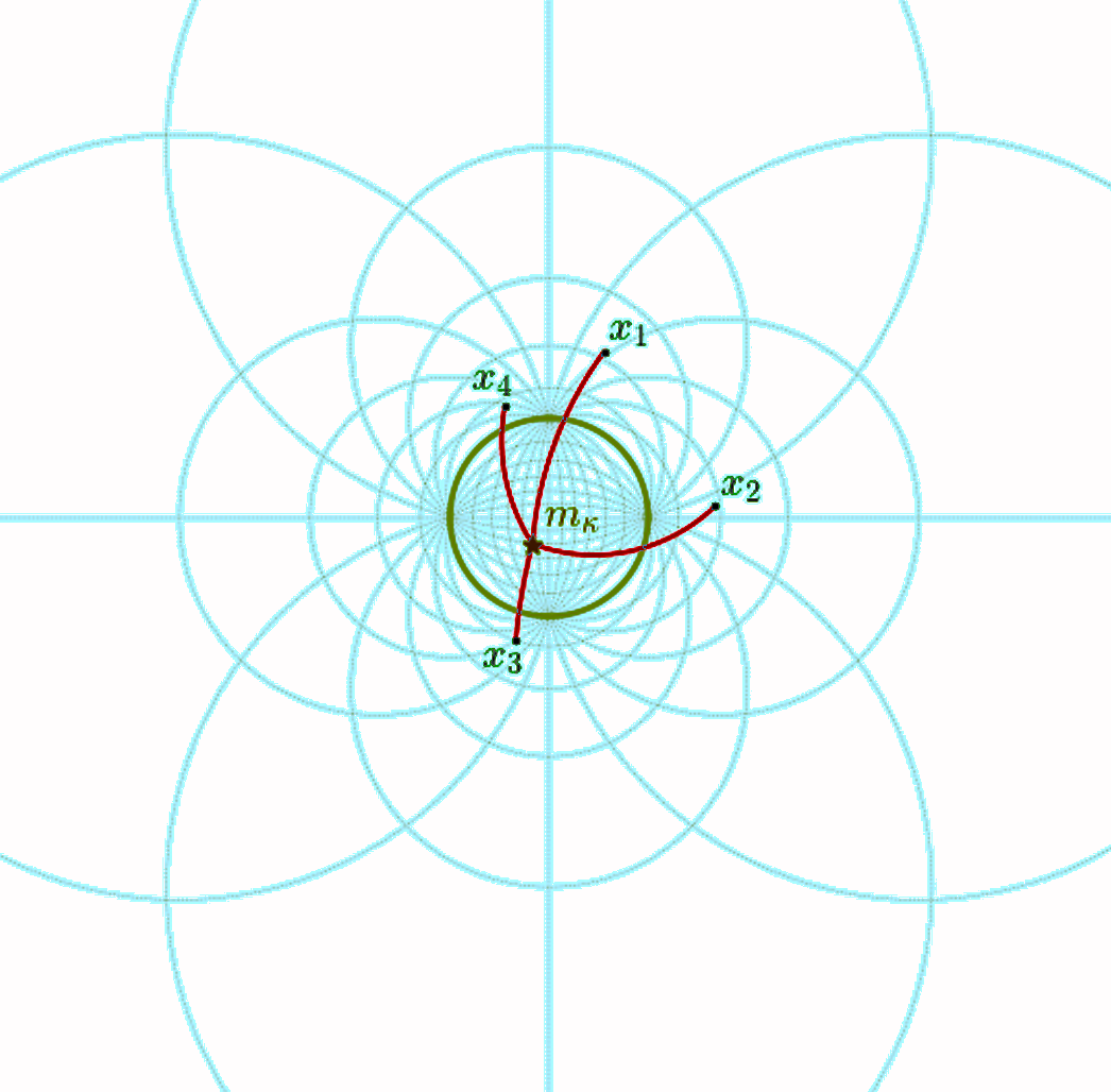
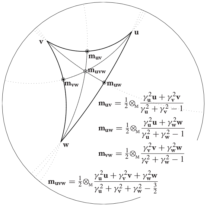
Figure 4: Left: Spherical gyromidpoint of four points. Right: Möbius gyromidpoint in the Poincaré model defined by (Ungar, 2008) and alternatively, here in eq. (12).

3.3 κ𝜅\kappa-Right-Matrix-Multiplication

Let 𝐗n×d𝐗superscript𝑛𝑑{\mathbf{X}}\in{\mathbb{R}}^{n\times d} denote a matrix whose n𝑛n rows are d𝑑d-dimensional embeddings in 𝔰𝔱κd𝔰subscriptsuperscript𝔱𝑑𝜅\mathfrak{st}^{d}_{\kappa}, and let 𝐖d×e𝐖superscript𝑑𝑒{\mathbf{W}}\in{\mathbb{R}}^{d\times e} denote a weight matrix. Let us first understand what a right matrix multiplication is in Euclidean space: the Euclidean right multiplication can be written row-wise as (𝐗𝐖)i=𝐗i𝐖subscript𝐗𝐖𝑖subscript𝐗𝑖𝐖({\mathbf{X}}{\mathbf{W}})_{i\bullet}={\mathbf{X}}_{i\bullet}{\mathbf{W}}. Hence each d𝑑d-dimensional Euclidean embedding is modified independently by a right matrix multiplication. A natural adaptation of this operation to the κ𝜅\kappa-stereographic model yields the following definition.

Definition 1.
Given a matrix 𝐗n×d𝐗superscript𝑛𝑑{\mathbf{X}}\in{\mathbb{R}}^{n\times d} holding κ𝜅\kappa-stereographic embeddings in its rows and weights 𝐖d×e𝐖superscript𝑑𝑒{\mathbf{W}}\in{\mathbb{R}}^{d\times e}, the κ𝜅\mathbf{\kappa}-right-matrix-multiplication is defined row-wise as (𝐗κ𝐖)i=exp0κ((log0κ(𝐗)𝐖)i)=tanκ(αitanκ1(𝐗i))(𝐗𝐖)i(𝐗𝐖)isubscriptsubscripttensor-product𝜅𝐗𝐖𝑖superscriptsubscript0𝜅subscriptsuperscriptsubscript0𝜅𝐗𝐖𝑖subscript𝜅subscript𝛼𝑖superscriptsubscript𝜅1normsubscript𝐗absent𝑖subscript𝐗𝐖𝑖normsubscript𝐗𝐖𝑖\begin{split}({\mathbf{X}}\otimes_{\kappa}{\mathbf{W}})_{i\bullet}&=\exp_{0}^{\kappa}\left((\log_{0}^{\kappa}({\mathbf{X}}){\mathbf{W}})_{i\bullet}\right)\\ &=\tan_{\kappa}\left(\alpha_{i}\tan_{\kappa}^{-1}(||{\mathbf{X}}_{\bullet i}||)\right)\frac{({\mathbf{X}}{\mathbf{W}})_{i\bullet}}{||({\mathbf{X}}{\mathbf{W}})_{i\bullet}||}\end{split} (10) where αi=(𝐗𝐖)i𝐗isubscript𝛼𝑖normsubscript𝐗𝐖𝑖normsubscript𝐗𝑖\alpha_{i}=\frac{||({\mathbf{X}}{\mathbf{W}})_{i\bullet}||}{||{\mathbf{X}}_{i\bullet}||} and exp0κsuperscriptsubscript0𝜅\exp_{0}^{\kappa} and log0κsuperscriptsubscript0𝜅\log_{0}^{\kappa} denote the exponential and logarithmic map in the κ𝜅\kappa-stereographic model.

This definition is in perfect agreement with the hyperbolic scalar multiplication for κ<0𝜅0\kappa<0, which can also be written as rκ𝐱=exp0κ(rlog0κ(𝐱))subscripttensor-product𝜅𝑟𝐱superscriptsubscript0𝜅𝑟superscriptsubscript0𝜅𝐱r\otimes_{\kappa}{\mathbf{x}}=\exp_{0}^{\kappa}(r\log_{0}^{\kappa}({\mathbf{x}})). This operation is known to have desirable properties such as associativity (Ganea et al., 2018a).

3.4 κ𝜅\kappa-Left-Matrix-Multiplication as a Midpoint Extension

For graph neural networks we also need the notion of message passing among neighboring nodes, i.e. an operation that combines / aggregates the respective embeddings together. In Euclidean space such an operation is given by the left multiplication of the embeddings matrix with the (preprocessed) adjacency 𝐀^^𝐀\hat{{\mathbf{A}}}: 𝐇(l+1)=σ(𝐀^𝐙(l))where𝐙(l)=𝐇(l)𝐖(l)superscript𝐇𝑙1𝜎^𝐀superscript𝐙𝑙wheresuperscript𝐙𝑙superscript𝐇𝑙superscript𝐖𝑙{\mathbf{H}}^{(l+1)}=\sigma(\hat{{\mathbf{A}}}{\mathbf{Z}}^{(l)})\ \text{where}\ {\mathbf{Z}}^{(l)}={\mathbf{H}}^{(l)}{\mathbf{W}}^{(l)}. Let us consider this left multiplication. For 𝐀n×n𝐀superscript𝑛𝑛{\mathbf{A}}\in{\mathbb{R}}^{n\times n}, the matrix product is given row-wise by:

(𝐀𝐗)i=Ai1𝐗1++Ain𝐗nsubscript𝐀𝐗𝑖subscript𝐴𝑖1subscript𝐗1subscript𝐴𝑖𝑛subscript𝐗𝑛({\mathbf{A}}{\mathbf{X}})_{i\bullet}=A_{i1}{\mathbf{X}}_{1\bullet}+\dots+A_{in}{\mathbf{X}}_{n\bullet}

This means that the new representation of node i𝑖i is obtained by calculating the linear combination of all the other node embeddings, weighted by the i𝑖i-th row of 𝐀𝐀{\mathbf{A}}. An adaptation to the κ𝜅\kappa-stereographic model hence requires a notion of weighted linear combination.

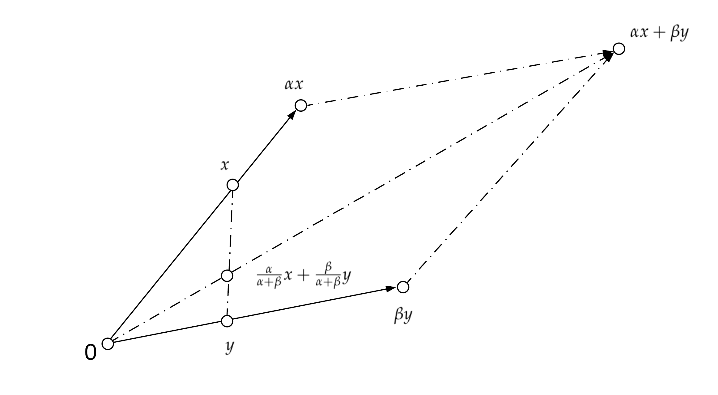
We propose such an operation in 𝔰𝔱κd𝔰subscriptsuperscript𝔱𝑑𝜅\mathfrak{st}^{d}_{\kappa} by performing a κ𝜅\kappa-scaling of a gyromidpoint - whose definition is reminded below. Indeed, in Euclidean space, the weighted linear combination α𝐱+β𝐲𝛼𝐱𝛽𝐲\alpha{\mathbf{x}}+\beta{\mathbf{y}} can be re-written as (α+β)m𝔼(𝐱,𝐲;α,β)𝛼𝛽subscript𝑚𝔼𝐱𝐲𝛼𝛽(\alpha+\beta)m_{\mathbb{E}}({\mathbf{x}},{\mathbf{y}};\alpha,\beta) with Euclidean midpoint m𝔼(𝐱,𝐲;α,β):=αα+β𝐱+βα+β𝐲assignsubscript𝑚𝔼𝐱𝐲𝛼𝛽𝛼𝛼𝛽𝐱𝛽𝛼𝛽𝐲m_{\mathbb{E}}({\mathbf{x}},{\mathbf{y}};\alpha,\beta):=\frac{\alpha}{\alpha+\beta}{\mathbf{x}}+\frac{\beta}{\alpha+\beta}{\mathbf{y}}. See fig. 5 for a geometric illustration. This motivates generalizing the above operation to 𝔰𝔱κd𝔰subscriptsuperscript𝔱𝑑𝜅\mathfrak{st}^{d}_{\kappa} as follows.

Definition 2.
Given a matrix 𝐗n×d𝐗superscript𝑛𝑑{\mathbf{X}}\in\mathbb{R}^{n\times d} holding κ𝜅\kappa-stereographic embeddings in its rows and weights 𝐀n×n𝐀superscript𝑛𝑛{\mathbf{A}}\in\mathbb{R}^{n\times n}, the κ𝜅\kappa-left-matrix-multiplication is defined row-wise as (𝐀κ𝐗)i:=(jAij)κmκ(𝐗1,,𝐗n;𝐀i).assignsubscriptsubscript𝜅𝐀𝐗𝑖subscripttensor-product𝜅subscript𝑗subscript𝐴𝑖𝑗subscript𝑚𝜅subscript𝐗1subscript𝐗𝑛subscript𝐀𝑖({\mathbf{A}}\boxtimes_{\kappa}{\mathbf{X}})_{i\bullet}:=(\sum_{j}A_{ij})\otimes_{\kappa}m_{\kappa}({\mathbf{X}}_{1\bullet},\cdots,{\mathbf{X}}_{n\bullet};{\mathbf{A}}_{i\bullet}). (11)
Refer to caption
Figure 5: Weighted Euclidean midpoint α𝐱+β𝐲𝛼𝐱𝛽𝐲\alpha{\bf x}+\beta{\bf y}
Refer to caption
Refer to caption
Figure 6: Heatmap of the distance from a 𝔰𝔱κ2𝔰subscriptsuperscript𝔱2𝜅\mathfrak{st}^{2}_{\kappa}-hyperplane to x𝔰𝔱κ2𝑥𝔰subscriptsuperscript𝔱2𝜅x\in\mathfrak{st}^{2}_{\kappa} for κ=0.254𝜅0.254\kappa=-0.254 (left) and κ=0.248𝜅0.248\kappa=0.248 (right)

The κ𝜅\kappa-scaling is motivated by the fact that dκ(𝟎,rκ𝐱)=|r|dκ(𝟎,𝐱)subscript𝑑𝜅0subscripttensor-product𝜅𝑟𝐱𝑟subscript𝑑𝜅0𝐱d_{\kappa}(\mathbf{0},r\otimes_{\kappa}{\mathbf{x}})=|r|d_{\kappa}(\mathbf{0},{\mathbf{x}}) for all r𝑟r\in\mathbb{R}, 𝐱𝔰𝔱κd𝐱𝔰superscriptsubscript𝔱𝜅𝑑{\mathbf{x}}\in\mathfrak{st}_{\kappa}^{d}. We remind that the gyromidpoint is defined when κ0𝜅0\kappa\leq 0 in the κ𝜅\kappa-stereographic model as (Ungar, 2010):

mκ(𝐱1,,𝐱n;𝜶)=12κ(i=1nαiλ𝐱iκj=1nαj(λ𝐱jκ1)𝐱i),subscript𝑚𝜅subscript𝐱1subscript𝐱𝑛𝜶subscripttensor-product𝜅12superscriptsubscript𝑖1𝑛subscript𝛼𝑖subscriptsuperscript𝜆𝜅subscript𝐱𝑖superscriptsubscript𝑗1𝑛subscript𝛼𝑗subscriptsuperscript𝜆𝜅subscript𝐱𝑗1subscript𝐱𝑖m_{\kappa}({\mathbf{x}}_{1},\cdots,{\mathbf{x}}_{n};\boldsymbol{\alpha})=\dfrac{1}{2}\otimes_{\kappa}\left(\sum_{i=1}^{n}\dfrac{\alpha_{i}\lambda^{\kappa}_{{\mathbf{x}}_{i}}}{\sum_{j=1}^{n}\alpha_{j}(\lambda^{\kappa}_{{\mathbf{x}}_{j}}-1)}{\mathbf{x}}_{i}\right), (12)

with λ𝐱κ=2/(1+κ𝐱2)subscriptsuperscript𝜆𝜅𝐱21𝜅superscriptnorm𝐱2\lambda^{\kappa}_{\mathbf{x}}=2/(1+\kappa\|{\mathbf{x}}\|^{2}). Whenever κ>0𝜅0\kappa>0, we have to further require the following condition:

jαj(λ𝐱jκ1)0.subscript𝑗subscript𝛼𝑗subscriptsuperscript𝜆𝜅subscript𝐱𝑗10\sum_{j}\alpha_{j}(\lambda^{\kappa}_{{\mathbf{x}}_{j}}-1)\neq 0. (13)

For two points, one can calculate that (λ𝐱κ1)+(λ𝐲κ1)=0superscriptsubscript𝜆𝐱𝜅1superscriptsubscript𝜆𝐲𝜅10(\lambda_{\mathbf{x}}^{\kappa}-1)+(\lambda_{\mathbf{y}}^{\kappa}-1)=0 is equivalent to κ𝐱𝐲=1𝜅norm𝐱norm𝐲1\kappa\|{\mathbf{x}}\|\|{\mathbf{y}}\|=1, which holds in particular whenever 𝐱=𝐲/(κ𝐲2)𝐱𝐲𝜅superscriptnorm𝐲2{\mathbf{x}}=-{\mathbf{y}}/(\kappa\|{\mathbf{y}}\|^{2}). See fig. 4 for illustrations of gyromidpoints.

Our operation κsubscript𝜅\boxtimes_{\kappa} satisfies interesting properties, proved in Appendix C.2.4:

Theorem 4 (Neuter element & κ𝜅\kappa-scalar-associativity).
We have 𝐈nκ𝐗=𝐗subscript𝜅subscript𝐈𝑛𝐗𝐗{\mathbf{I}}_{n}\boxtimes_{\kappa}{\mathbf{X}}={\mathbf{X}}, and for r𝑟r\in\mathbb{R}, rκ(𝐀κ𝐗)=(r𝐀)κ𝐗.subscripttensor-product𝜅𝑟subscript𝜅𝐀𝐗subscript𝜅𝑟𝐀𝐗r\otimes_{\kappa}({\mathbf{A}}\boxtimes_{\kappa}{\mathbf{X}})=(r{\mathbf{A}})\boxtimes_{\kappa}{\mathbf{X}}.
The matrix 𝐀𝐀{\mathbf{A}}.

In most GNNs, the matrix 𝐀𝐀{\mathbf{A}} is intended to be a preprocessed adjacency matrix, i.e. renormalized by the diagonal degree matrix 𝐃ii=kAiksubscript𝐃𝑖𝑖subscript𝑘subscript𝐴𝑖𝑘{\mathbf{D}}_{ii}=\sum_{k}A_{ik}. This normalization is often taken either (i) to the left: 𝐃1𝐀superscript𝐃1𝐀{\mathbf{D}}^{-1}{\mathbf{A}}, (ii) symmetric: 𝐃12𝐀𝐃12superscript𝐃12superscript𝐀𝐃12{\mathbf{D}}^{-\frac{1}{2}}{\mathbf{A}}{\mathbf{D}}^{-\frac{1}{2}} or (iii) to the right: 𝐀𝐃1superscript𝐀𝐃1{\mathbf{A}}{\mathbf{D}}^{-1}. Note that the latter case makes the matrix right-stochastic222𝐌𝐌{\mathbf{M}} is right-stochastic if for all i𝑖i, jMij=1subscript𝑗subscript𝑀𝑖𝑗1\sum_{j}M_{ij}=1., which is a property that is preserved by matrix product and exponentiation. For this case, we prove the following result in Appendix C.2.5:

Theorem 5 (κ𝜅\kappa-left-multiplication by right-stochastic matrices is intrinsic).
If 𝐀,𝐁𝐀𝐁{\mathbf{A}},{\mathbf{B}} are right-stochastic, ϕitalic-ϕ\phi is a isometry of 𝔰𝔱κd𝔰subscriptsuperscript𝔱𝑑𝜅\mathfrak{st}^{d}_{\kappa} and 𝐗𝐗{\mathbf{X}},𝐘𝐘{\mathbf{Y}} are two matrices holding κ𝜅\kappa-stereographic embeddings: i,dϕ=dκ((𝐀κϕ(𝐗))i,(𝐁κϕ(𝐘))i)=dκ((𝐀κ𝐗)i,(𝐁κ𝐘)i).\begin{split}\forall i,\quad d_{\phi}&=d_{\kappa}\left(({\mathbf{A}}\boxtimes_{\kappa}\phi({\mathbf{X}}))_{i\bullet},({\mathbf{B}}\boxtimes_{\kappa}\phi({\mathbf{Y}}))_{i\bullet}\right)\\ &=d_{\kappa}(({\mathbf{A}}\boxtimes_{\kappa}{\mathbf{X}})_{i\bullet},({\mathbf{B}}\boxtimes_{\kappa}{\mathbf{Y}})_{i\bullet}).\end{split} (14)

The above result means that 𝐀𝐀{\mathbf{A}} can easily be preprocessed as to make its κ𝜅\kappa-left-multiplication intrinsic to the metric space (𝔰𝔱κd𝔰superscriptsubscript𝔱𝜅𝑑\mathfrak{st}_{\kappa}^{d}, dκsubscript𝑑𝜅d_{\kappa}). At this point, one could wonder: does there exist other ways to take weighted centroids on a Riemannian manifold? We comment on two plausible alternatives.

Fréchet/Karcher means.

They are obtained as argmin𝐱iαidκ(𝐱,𝐱i)2subscript𝐱subscript𝑖subscript𝛼𝑖subscript𝑑𝜅superscript𝐱subscript𝐱𝑖2\arg\min_{\mathbf{x}}\sum_{i}\alpha_{i}d_{\kappa}({\mathbf{x}},{\mathbf{x}}_{i})^{2}; note that although they are also intrinsic, they usually require solving an optimization problem which can be prohibitively expensive, especially when one requires gradients to flow through the solution - moreover, for the space 𝔰𝔱κd𝔰superscriptsubscript𝔱𝜅𝑑\mathfrak{st}_{\kappa}^{d}, it is known that the minimizer is unique if and only if κ0𝜅0\kappa\geq 0.

Tangential aggregations.

The linear combination is here lifted to the tangent space by means of the exponential and logarithmic map and were in particular used in the recent works of Chami et al. (2019) and Liu et al. (2019).

Definition 3.
The tangential aggregation of 𝐱1,,𝐱n𝔰𝔱κdsubscript𝐱1subscript𝐱𝑛𝔰subscriptsuperscript𝔱𝑑𝜅{\mathbf{x}}_{1},\dots,{\mathbf{x}}_{n}\in\mathfrak{st}^{d}_{\kappa} w.r.t. weights {αi}1insubscriptsubscript𝛼𝑖1𝑖𝑛\{\alpha_{i}\}_{1\leq i\leq n}, at point 𝐱𝔰𝔱κd𝐱𝔰subscriptsuperscript𝔱𝑑𝜅{\mathbf{x}}\in\mathfrak{st}^{d}_{\kappa} (for 𝐱i𝐱/(κ𝐱2)subscript𝐱𝑖𝐱𝜅superscriptnorm𝐱2{\mathbf{x}}_{i}\neq-{\mathbf{x}}/(\kappa\|{\mathbf{x}}\|^{2}) if κ>0𝜅0\kappa>0) is defined by: 𝔱𝔤𝐱κ(𝐱1,,𝐱n;α1,,αn):=exp𝐱κ(i=1nαilog𝐱κ(𝐱i)).assign𝔱superscriptsubscript𝔤𝐱𝜅subscript𝐱1subscript𝐱𝑛subscript𝛼1subscript𝛼𝑛superscriptsubscript𝐱𝜅superscriptsubscript𝑖1𝑛subscript𝛼𝑖superscriptsubscript𝐱𝜅subscript𝐱𝑖\mathfrak{tg}_{\mathbf{x}}^{\kappa}({\mathbf{x}}_{1},...,{\mathbf{x}}_{n};\alpha_{1},...,\alpha_{n}):=\exp_{\mathbf{x}}^{\kappa}\left(\sum_{i=1}^{n}\alpha_{i}\log_{\mathbf{x}}^{\kappa}({\mathbf{x}}_{i})\right). (15)

The below theorem describes that for the κ𝜅\kappa-stereographic model, this operation is also intrinsic. We prove it in Appendix C.2.6.

Theorem 6 (Tangential aggregation is intrinsic).
For any isometry ϕitalic-ϕ\phi of 𝔰𝔱κd𝔰superscriptsubscript𝔱𝜅𝑑\mathfrak{st}_{\kappa}^{d}, we have 𝔱𝔤ϕ(𝐱)({ϕ(𝐱i)};{αi})=ϕ(𝔱𝔤𝐱({𝐱i};{αi})).𝔱subscript𝔤italic-ϕ𝐱italic-ϕsubscript𝐱𝑖subscript𝛼𝑖italic-ϕ𝔱subscript𝔤𝐱subscript𝐱𝑖subscript𝛼𝑖\mathfrak{tg}_{\phi({\mathbf{x}})}(\{\phi({\mathbf{x}}_{i})\};\{\alpha_{i}\})=\phi(\mathfrak{tg}_{{\mathbf{x}}}(\{{\mathbf{x}}_{i}\};\{\alpha_{i}\})). (16)

3.5 Logits

Finally, we need the logit and softmax layer, a neccessity for any classification task. We here use the model of Ganea et al. (2018a), which was obtained in a principled manner for the case of negative curvature. Their derivation rests upon the closed-form formula for distance to a hyperbolic hyperplane. We naturally extend this formula to 𝔰𝔱κd𝔰subscriptsuperscript𝔱𝑑𝜅\mathfrak{st}^{d}_{\kappa}, hence also allowing for κ>0𝜅0\kappa>0 but leave for future work the adaptation of their theoretical analysis.

p(y=k|𝐱)=S(𝐚k𝐩k|κ|sinκ1(2|κ|𝐳k,𝐚k(1+κ𝐳k2)𝐚k)),𝑝𝑦conditional𝑘𝐱Ssubscriptnormsubscript𝐚𝑘subscript𝐩𝑘𝜅superscriptsubscript𝜅12𝜅subscript𝐳𝑘subscript𝐚𝑘1𝜅superscriptnormsubscript𝐳𝑘2normsubscript𝐚𝑘p(y=k|{\mathbf{x}})=\text{S}\left(\frac{||\mathbf{a}_{k}||_{\mathbf{p}_{k}}}{\sqrt{|\kappa|}}\sin_{\kappa}^{-1}\left(\frac{2\sqrt{|\kappa|}\langle{\mathbf{z}}_{k},\mathbf{a}_{k}\rangle}{(1+\kappa||{\mathbf{z}}_{k}||^{2})||\mathbf{a}_{k}||}\right)\right), (17)

where 𝐚k𝒯0𝔰𝔱κddsubscript𝐚𝑘subscript𝒯0𝔰superscriptsubscript𝔱𝜅𝑑superscript𝑑\mathbf{a}_{k}\in\mathcal{T}_{0}\mathfrak{st}_{\kappa}^{d}\cong{\mathbb{R}}^{d} and 𝐩k𝔰𝔱κdsubscript𝐩𝑘𝔰subscriptsuperscript𝔱𝑑𝜅\mathbf{p}_{k}\in\mathfrak{st}^{d}_{\kappa} are trainable parameters, 𝐱𝔰𝔱κd,𝐱𝔰superscriptsubscript𝔱𝜅𝑑{\mathbf{x}}\in\mathfrak{st}_{\kappa}^{d}\ \mathrm{,}\ is the input,
zk=𝐩k𝐱subscript𝑧𝑘direct-sumsubscript𝐩𝑘𝐱z_{k}=-\mathbf{p}_{k}\oplus{\mathbf{x}} and S()S\text{S}(\cdot) is the softmax function.
We reference the reader to Appendix D for further details and to fig. 6 for an illustration of eq. 17.

3.6 κ𝜅\kappa-GCN

We are now ready to introduce our κ𝜅\kappa-stereographic GCN (Kipf & Welling, 2017), denoted by κ𝜅\kappa-GCN333To be pronounced “kappa” GCN; the greek letter κ𝜅\kappa being commonly used to denote sectional curvature. Assume we are given a graph with node level features G=(V,𝐀,𝐗)𝐺𝑉𝐀𝐗G=(V,{\mathbf{A}},{\mathbf{X}}) where 𝐗n×d𝐗superscript𝑛𝑑{\mathbf{X}}\in{\mathbb{R}}^{n\times d} with each row 𝐗i𝔰𝔱κdsubscript𝐗𝑖𝔰superscriptsubscript𝔱𝜅𝑑{\mathbf{X}}_{i\bullet}\in\mathfrak{st}_{\kappa}^{d} and adjacency 𝐀n×n𝐀superscript𝑛𝑛{\mathbf{A}}\in{\mathbb{R}}^{n\times n}. We first perform a preprocessing step by mapping the Euclidean features to 𝔰𝔱κd𝔰superscriptsubscript𝔱𝜅𝑑\mathfrak{st}_{\kappa}^{d} via the projection 𝐗𝐗/(2|κ|𝐗max)maps-to𝐗𝐗2𝜅subscriptnorm𝐗{\mathbf{X}}\mapsto{\mathbf{X}}/(2\sqrt{|\kappa|}||{\mathbf{X}}||_{\max}), where 𝐗maxsubscriptnorm𝐗||{\mathbf{X}}||_{\max} denotes the maximal Euclidean norm among all stereographic embeddings in 𝐗𝐗{\mathbf{X}}. For l{0,,L2}𝑙0𝐿2l\in\{0,\dots,L-2\}, the (l+1)𝑙1(l+1)-th layer of κ𝜅\kappa-GCN is given by:

𝐇(l+1)=σκ(𝐀^κ(𝐇(l)κ𝐖(l))),superscript𝐇𝑙1superscript𝜎subscripttensor-product𝜅subscript𝜅^𝐀subscripttensor-product𝜅superscript𝐇𝑙superscript𝐖𝑙{\mathbf{H}}^{(l+1)}=\sigma^{\otimes_{\kappa}}\left(\hat{{\mathbf{A}}}\boxtimes_{\kappa}\left({\mathbf{H}}^{(l)}\otimes_{\kappa}{\mathbf{W}}^{(l)}\right)\right), (18)

where 𝐇(0)=𝐗superscript𝐇0𝐗{\mathbf{H}}^{(0)}={\mathbf{X}}, σκ(𝐱):=exp𝟎κ(σ(log𝟎κ(𝐱)))assignsuperscript𝜎subscripttensor-product𝜅𝐱subscriptsuperscript𝜅0𝜎superscriptsubscript0𝜅𝐱\sigma^{\otimes_{\kappa}}({\mathbf{x}}):=\exp^{\kappa}_{\mathbf{0}}(\sigma(\log_{\mathbf{0}}^{\kappa}({\mathbf{x}}))) is the Möbius version (Ganea et al., 2018a) of a pointwise non-linearity σ𝜎\sigma and 𝐀^=𝐃~12𝐀~𝐃~12^𝐀superscript~𝐃12~𝐀superscript~𝐃12\hat{{\mathbf{A}}}=\tilde{{\mathbf{D}}}^{-\frac{1}{2}}\tilde{{\mathbf{A}}}\tilde{{\mathbf{D}}}^{-\frac{1}{2}}. The final layer is a κ𝜅\kappa-logit layer (Appendix D):

𝐇(L)=softmax(𝐀^logitκ(𝐇(L1),𝐖(L1))),superscript𝐇𝐿softmax^𝐀subscriptlogit𝜅superscript𝐇𝐿1superscript𝐖𝐿1{\mathbf{H}}^{(L)}=\text{softmax}\left(\hat{{\mathbf{A}}}\ \text{logit}_{\kappa}\left({\mathbf{H}}^{(L-1)},{\mathbf{W}}^{(L-1)}\right)\right), (19)

where 𝐖(L1)superscript𝐖𝐿1{\mathbf{W}}^{(L-1)} contains the parameters 𝐚ksubscript𝐚𝑘\mathbf{a}_{k} and 𝐩ksubscript𝐩𝑘\mathbf{p}_{k} of the κ𝜅\kappa-logits layer. A very important property of κ𝜅\kappa-GCN is that its architecture recovers the Euclidean GCN when we let curvature go to zero:

κ-GCNκ0GCN.absent𝜅0𝜅-GCNGCN\kappa\text{-GCN}\xrightarrow{\kappa\xrightarrow{}0}\text{GCN}.

4 Experiments

We evaluate the architectures introduced in the previous sections on the tasks of node classification and minimizing embedding distortion for several synthetic as well as real datasets. We detail the training setup and model architecture choices to Appendix F.

Table 1: Minimum achieved average distortion of the different models. \mathbb{H} and 𝕊𝕊\mathbb{S} denote hyperbolic and spherical models respectively.

Model Tree Toroidal Spherical
𝔼10superscript𝔼10\mathbb{E}^{10} (Linear) 0.045 0.0607 0.0415
𝔼10superscript𝔼10\mathbb{E}^{10} (ReLU) 0.0502 0.0603 0.0409
10superscript10\mathbb{H}^{10} (κ𝜅\kappa-GCN) 0.0029 0.272 0.267
𝕊10superscript𝕊10\mathbb{S}^{10} (κ𝜅\kappa-GCN) 0.473 0.0485 0.0337
5×5superscript5superscript5\mathbb{H}^{5}\times\mathbb{H}^{5} (κ𝜅\kappa-GCN) 0.0048 0.112 0.152
𝕊5×𝕊5superscript𝕊5superscript𝕊5\mathbb{S}^{5}\times\mathbb{S}^{5} (κ𝜅\kappa-GCN) 0.51 0.0464 0.0359
(2)4superscriptsuperscript24\left(\mathbb{H}^{2}\right)^{4} (κ𝜅\kappa-GCN) 0.025 0.084 0.062
(𝕊2)4superscriptsuperscript𝕊24\left(\mathbb{S}^{2}\right)^{4} (κ𝜅\kappa-GCN) 0.312 0.0481 0.0378
Table 2: Node classification: Average accuracy across 5 splits with estimated uncertainties at 95 percent confidence level via bootstrapping on our datasplits. \mathbb{H} and 𝕊𝕊\mathbb{S} denote hyperbolic and spherical models respectively.

Model Citeseer Cora Pubmed Airport
𝔼16superscript𝔼16\mathbb{E}^{16} (Kipf & Welling, 2017) 0.729±0.0054plus-or-minus0.7290.00540.729\pm 0.0054 0.814±0.004plus-or-minus0.8140.0040.814\pm 0.004 0.792±0.0039plus-or-minus0.7920.00390.792\pm 0.0039 0.814±0.0029plus-or-minus0.8140.00290.814\pm 0.0029
16superscript16\mathbb{H}^{16} (Chami et al., 2019) 0.71±0.0049plus-or-minus0.710.00490.71\pm 0.0049 0.803±0.0046plus-or-minus0.8030.00460.803\pm 0.0046 0.798±0.0043plus-or-minus0.7980.0043\textbf{0.798}\pm\textbf{0.0043}\textbf{} 0.844±0.0041plus-or-minus0.8440.0041\textbf{0.844}\pm\textbf{0.0041}
16superscript16\mathbb{H}^{16} (κ𝜅\kappa-GCN) 0.732±0.0051plus-or-minus0.7320.0051\textbf{0.732}\pm\textbf{0.0051} 0.812±0.005plus-or-minus0.8120.0050.812\pm 0.005 0.785±0.0036plus-or-minus0.7850.00360.785\pm 0.0036 0.819±0.0033plus-or-minus0.8190.00330.819\pm 0.0033
𝕊16superscript𝕊16\mathbb{S}^{16} (κ𝜅\kappa-GCN) 0.721±0.0045plus-or-minus0.7210.00450.721\pm 0.0045 0.819±0.0045plus-or-minus0.8190.0045\textbf{0.819}\pm\textbf{0.0045} 0.788±0.0049plus-or-minus0.7880.00490.788\pm 0.0049 0.809±0.0058plus-or-minus0.8090.00580.809\pm 0.0058
Prod-GCN (κ𝜅\kappa-GCN) 0.711±0.0059plus-or-minus0.7110.00590.711\pm 0.0059 0.808±0.0041plus-or-minus0.8080.00410.808\pm 0.0041 0.781±0.006plus-or-minus0.7810.0060.781\pm 0.006 0.817±0.0044plus-or-minus0.8170.00440.817\pm 0.0044
Minimizing Distortion

Our first goal is to evaluate the graph embeddings learned by our GCN models on the representation task of fitting the graph metric in the embedding space. We desire to minimize the average distortion, i.e. defined similarly as in Gu et al. (2019): 1n2i,j((d(𝐱i,𝐱j)dG(i,j))21)21superscript𝑛2subscript𝑖𝑗superscriptsuperscript𝑑subscript𝐱𝑖subscript𝐱𝑗subscript𝑑𝐺𝑖𝑗212\frac{1}{n^{2}}\sum_{i,j}\left(\left(\frac{d({\mathbf{x}}_{i},{\mathbf{x}}_{j})}{d_{G}(i,j)}\right)^{2}-1\right)^{2}, where d(𝐱i,𝐱j)𝑑subscript𝐱𝑖subscript𝐱𝑗d({\mathbf{x}}_{i},{\mathbf{x}}_{j}) is the distance between the embeddings of nodes i and j, while dG(i,j)subscript𝑑𝐺𝑖𝑗d_{G}(i,j) is their graph distance (shortest path length).

We create three synthetic datasets that best reflect the different geometries of interest: i) “Tree‘”: a balanced tree of depth 5 and branching factor 4 consisting of 1365 nodes and 1364 edges. ii) “Torus”: We sample points (nodes) from the (planar) torus, i.e. from the unit connected square; two nodes are connected by an edge if their toroidal distance (the warped distance) is smaller than a fixed R=0.01𝑅0.01R=0.01; this gives 1000 nodes and 30626 edges. iii) “Spherical Graph”: we sample points (nodes) from 𝕊2superscript𝕊2{\mathbb{S}}^{2}, connecting nodes if their distance is smaller than 0.2, leading to 1000 nodes and 17640 edges.

For the GCN models, we use 1-hot initial node features. We use two GCN layers with dimensions 16 and 10. The non-Euclidean models do not use additional non-linearities between layers. All Euclidean parameters are updated using the ADAM optimizer with learning rate 0.01. Curvatures are learned using gradient descent and learning rate of 0.0001. All models are trained for 10000 epochs and we report the minimal achieved distortion.

Distortion results.

The obtained distortion scores shown in table 1 reveal the benefit of our models. The best performing architecture is the one that matches the underlying geometry of the graph.
Refer to caption
Refer to caption
Refer to caption
Refer to caption
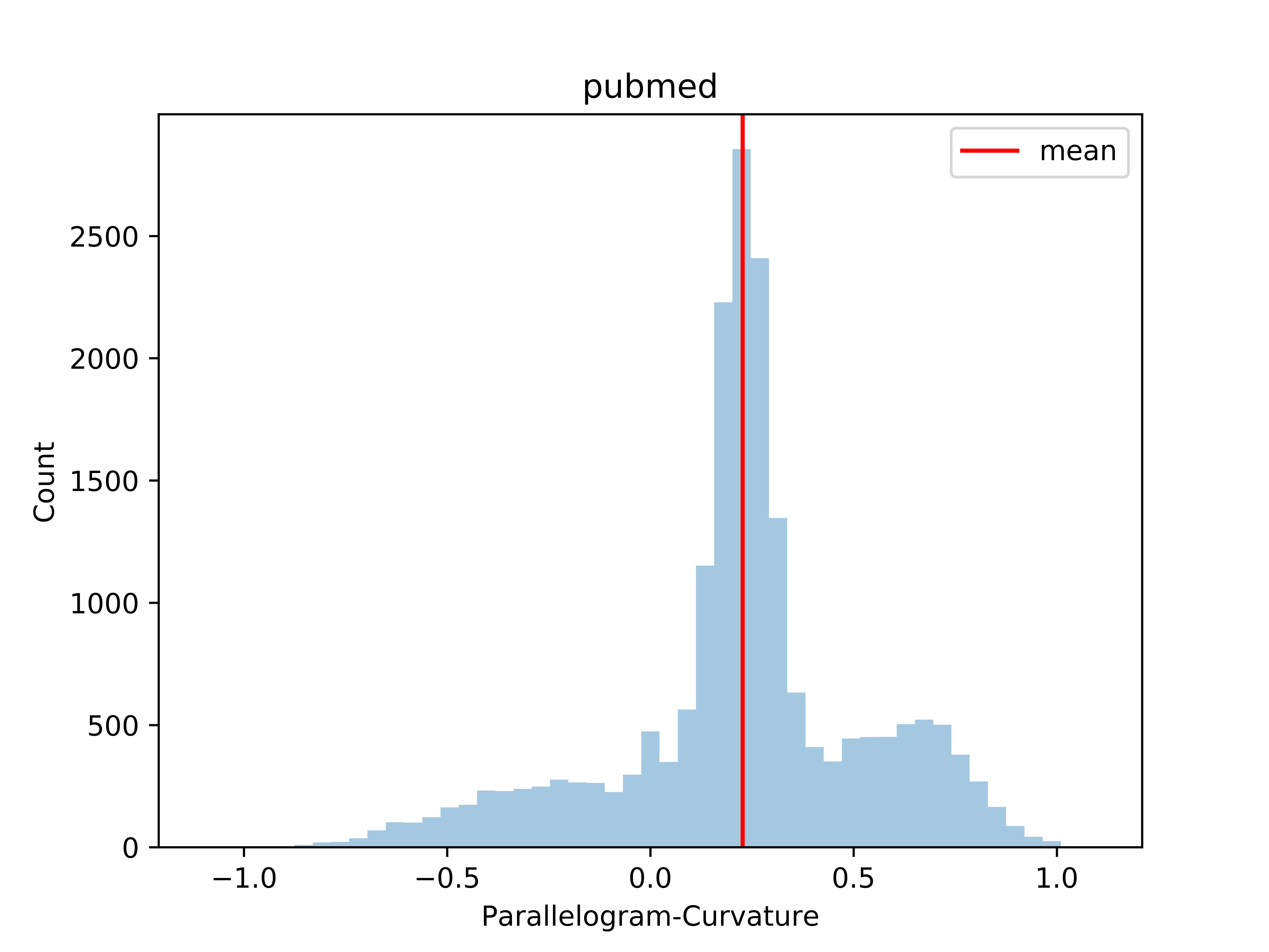
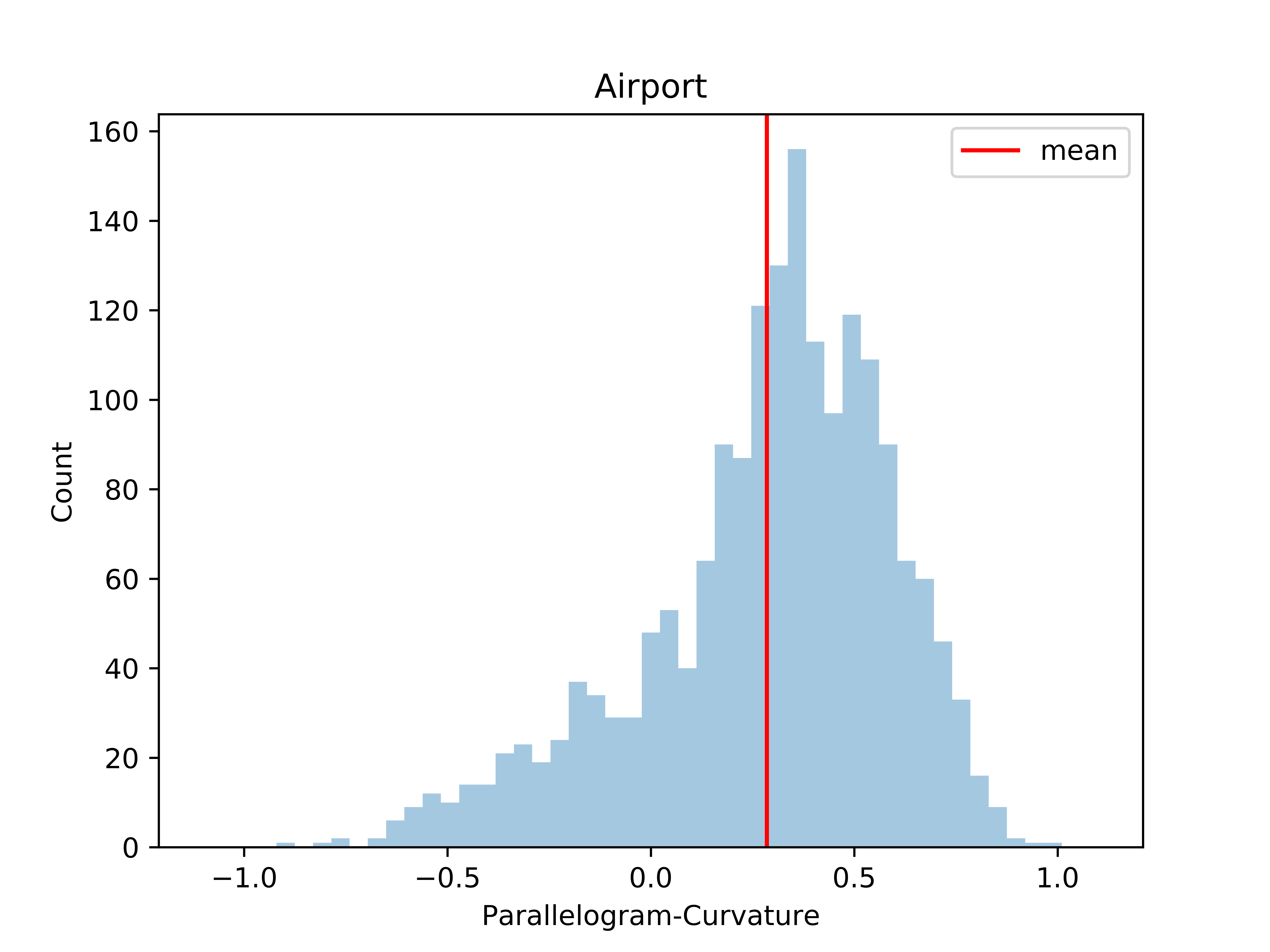
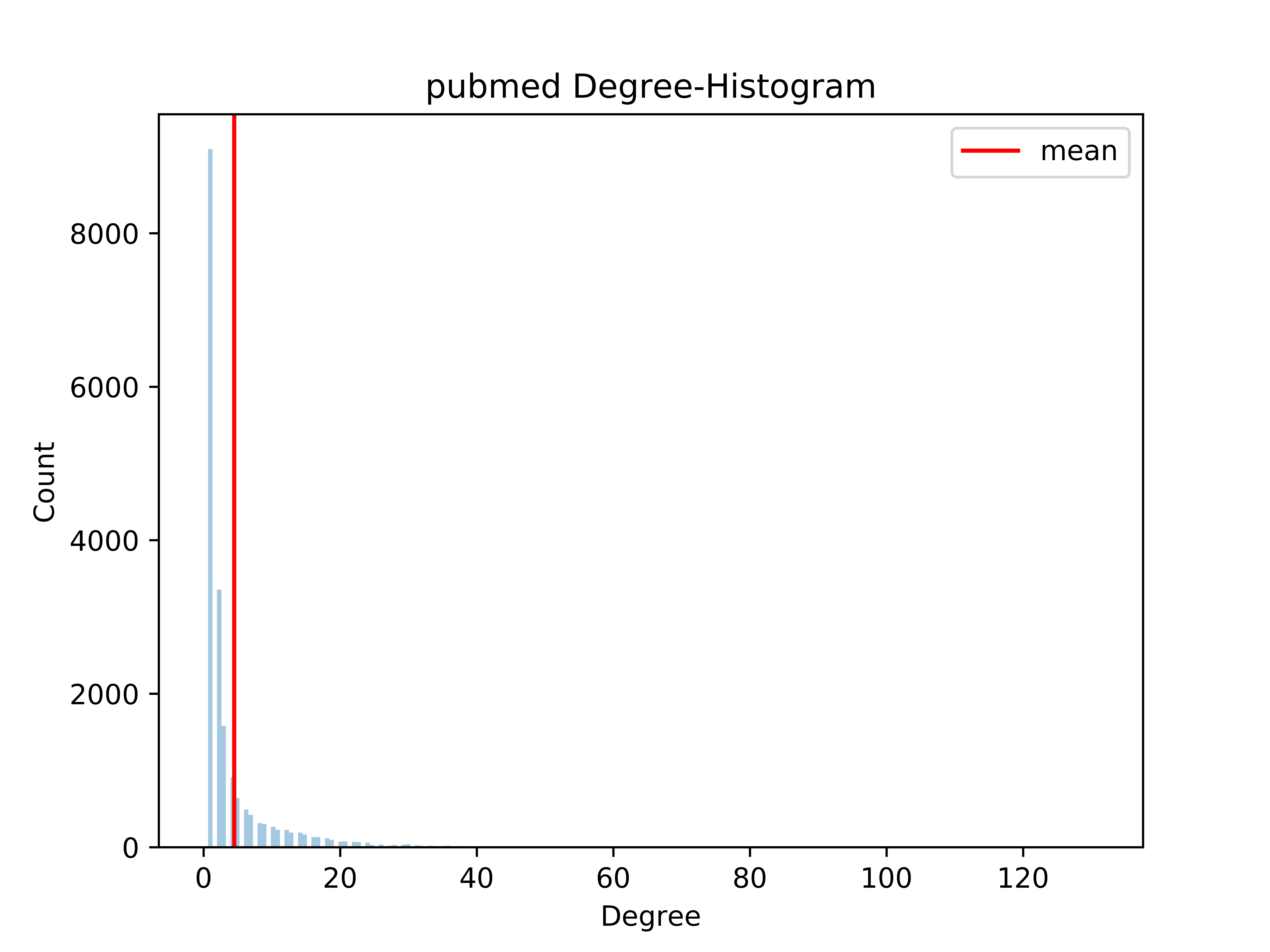
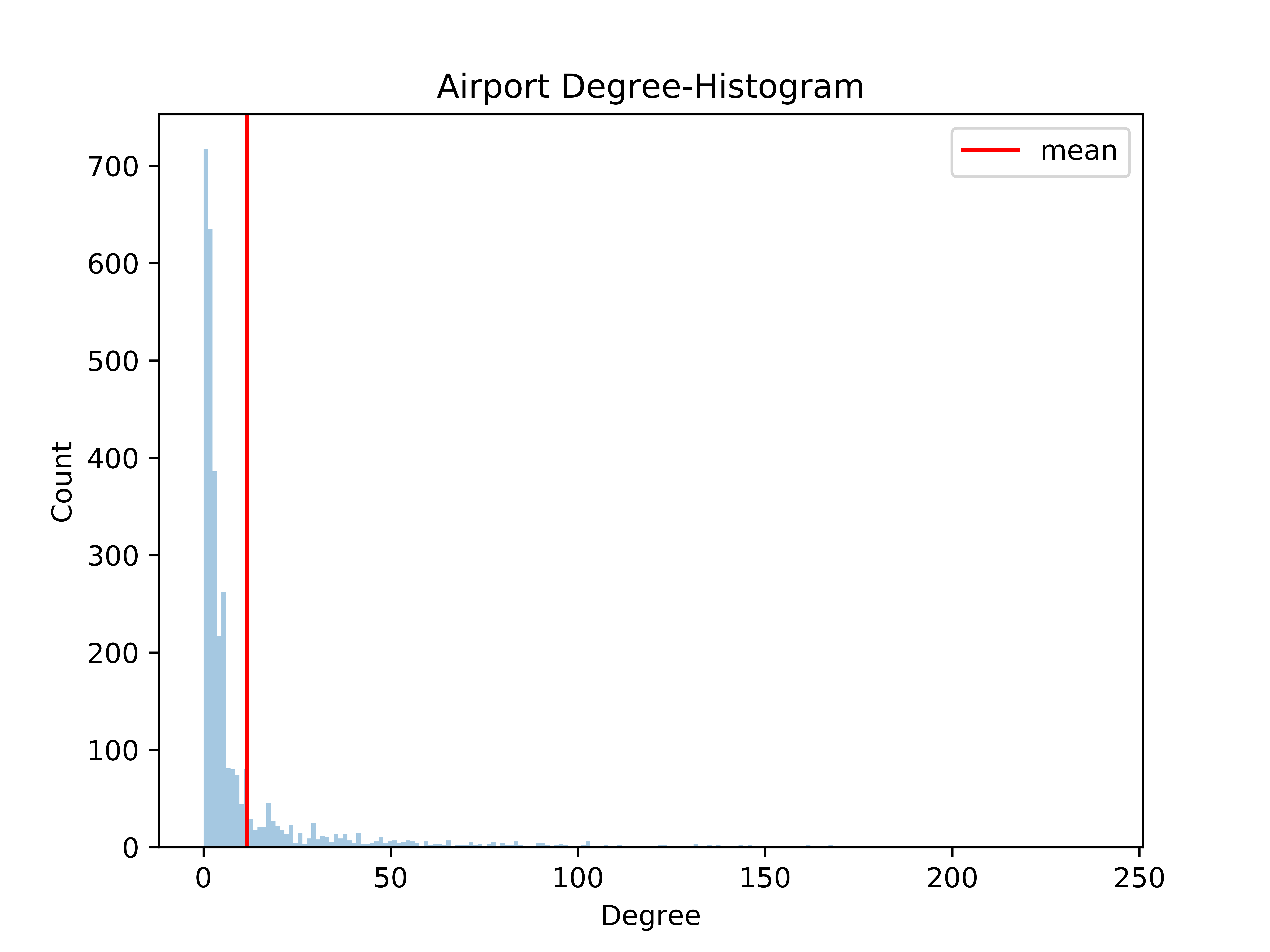
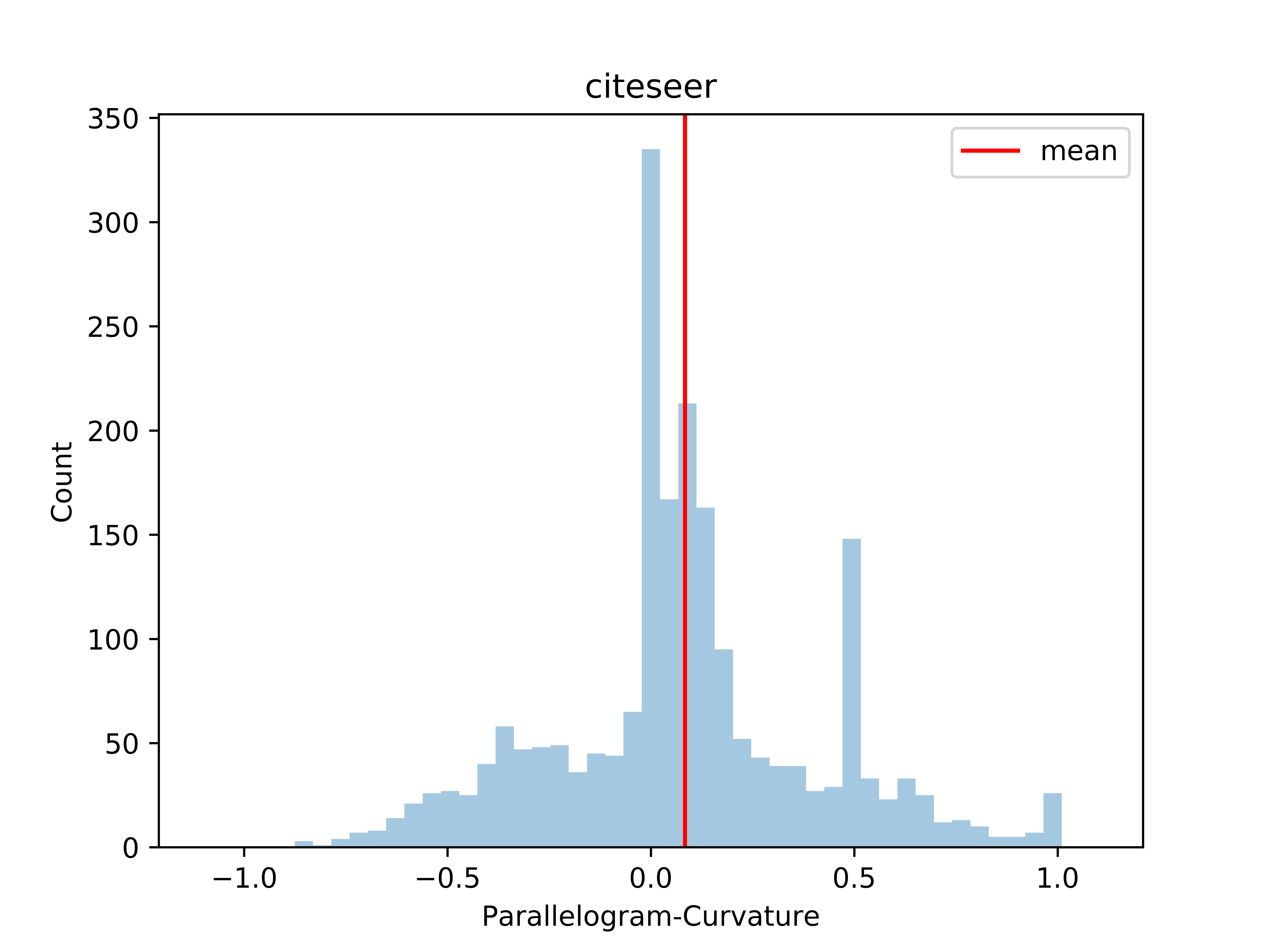
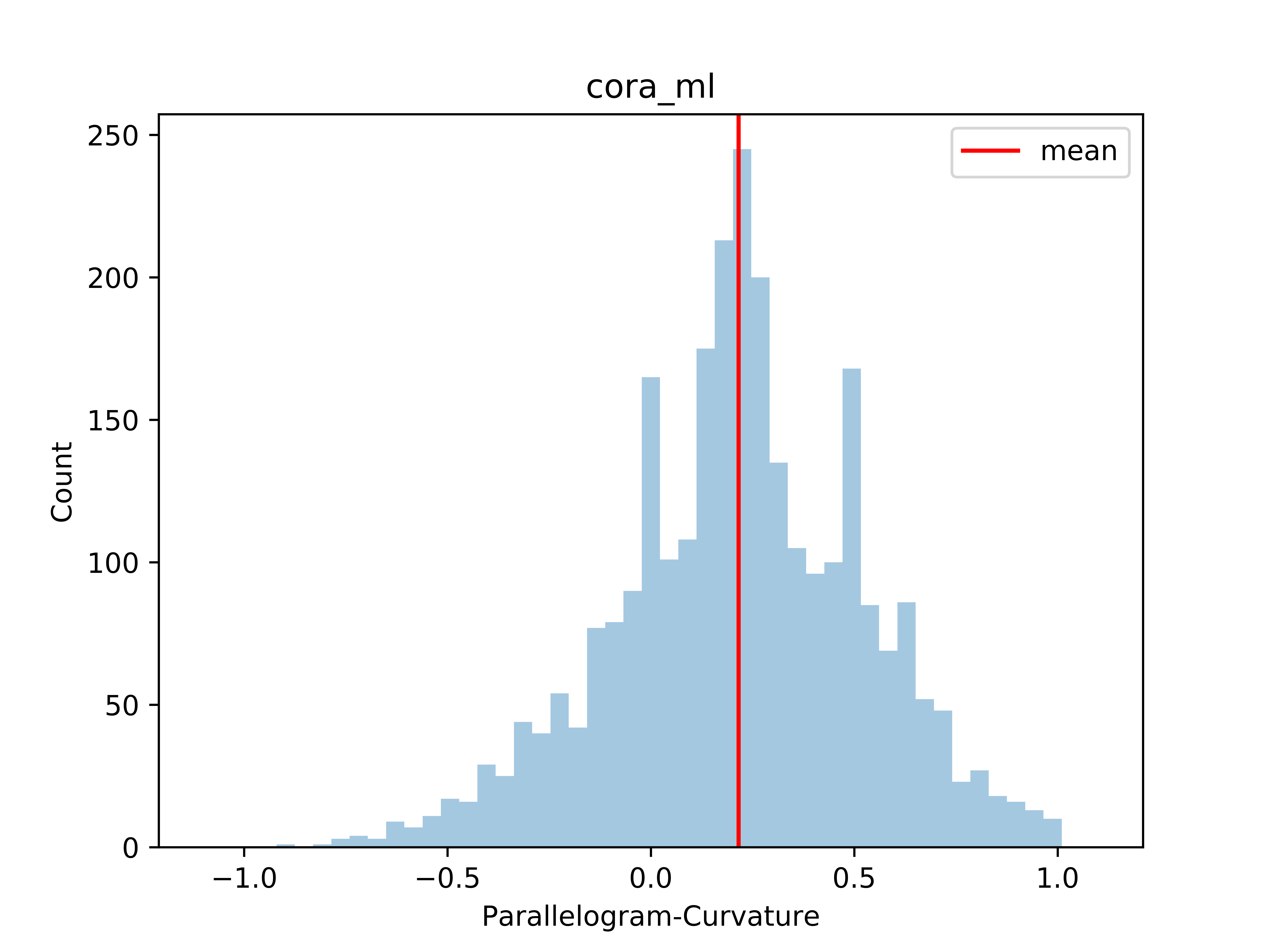
Figure 7: Histogram of Curvatures from ”Deviation of Parallogram Law”

4.1 Node Classification

We consider the popular node classification datasets Citeseer (Sen et al., 2008), Cora-ML (McCallum et al., 2000) and Pubmed (Namata et al., 2012). Node labels correspond to the particular subfield the published document is associated with. Dataset statistics and splitting details are deferred to the Appendix F due to the lack of space. We compare against the Euclidean model (Kipf & Welling, 2017) and the recently proposed hyperbolic variant (Chami et al., 2019).

Curvature Estimations of Datasets

To understand how far are the real graphs of the above datasets from the Euclidean geometry, we first estimate the graph curvature of the four studied datasets using the deviation from the Parallelogram Law (Gu et al., 2019) as detailed in Appendix G. Curvature histograms are shown in fig. 7. It can be noticed that the datasets are mostly non-Euclidean, thus offering a good motivation to apply our constant-curvature GCN architectures.

Training Details

We trained the baseline models in the same setting as done in Chami et al. (2019). Namely, for GCN we use one hidden layer of size 16, dropout on the embeddings and the adjacency of rate 0.50.50.5 as well as L2superscript𝐿2L^{2}-regularization for the weights of the first layer. We used ReLU as the non-linear activation function.

For the non-Euclidean architectures, we used a combination of dropout and dropconnect for the non-Euclidean models as reported in Chami et al. (2019), as well as L2superscript𝐿2L^{2}-regularization for the first layer. All models have the same number of parameters and for fairness are compared in the same setting, without attention. We use one hidden layer of dimension 16. For the product models we consider two-component spaces (e.g 8×𝕊8superscript8superscript𝕊8\mathbb{H}^{8}\times\mathbb{S}^{8}) and we split the embedding space into equal dimensions of size 8. We also distribute the input features equally among the components. Non-Euclidean models use the Möbius version of ReLU. Euclidean parameters use a learning rate of 0.01 for all models using ADAM. The curvatures are learned using gradient descent with a learning rate of 0.01. We show the learnt values in Appendix F. We use early stopping: we first train for 2000 epochs, then we check every 200 epochs for improvement in the validation cross entropy loss; if that is not observed, we stop.

Node classification results.

These are shown in table 2. It can be seen that our models are competitive with the Euclidean GCN considered and outperforms Chami et al. (2019) on Citeseer and Cora, showcasing the benefit of our proposed architecture.

5 Conclusion

In this paper, we introduced a natural extension of GCNs to the stereographic models of both positive and negative curvatures in a unified manner. We show how this choice of models permits a differentiable interpolation between positive and negative curvature, allowing the curvature to be trained independent of an initial sign choice. We hope that our models will open new exciting directions into non-Euclidean graph neural networks.

6 Acknowledgements

We thank prof. Thomas Hofmann, Andreas Bloch, Calin Cruceru and Ondrej Skopek for useful discussions and anonymous reviewers for suggestions.
Gary Bécigneul is funded by the Max Planck ETH Center for Learning Systems.

References

  • Abu-El-Haija et al. (2018) Abu-El-Haija, S., Kapoor, A., Perozzi, B., and Lee, J. N-GCN: Multi-scale Graph Convolution for Semi-supervised Node Classification. International Workshop on Mining and Learning with Graphs (MLG), 2018.
  • Amari & Nagaoka (2007) Amari, S.-i. and Nagaoka, H. Methods of information geometry, volume 191. American Mathematical Soc., 2007.
  • Bahdanau et al. (2015) Bahdanau, D., Cho, K., and Bengio, Y. Neural machine translation by jointly learning to align and translate. Proceedings of the International Conference on Learning Representations, 2015.
  • Bronstein et al. (2017) Bronstein, M. M., Bruna, J., LeCun, Y., Szlam, A., and Vandergheynst, P. Geometric deep learning: going beyond euclidean data. IEEE Signal Processing Magazine, 34(4):18–42, 2017.
  • Bruna et al. (2014) Bruna, J., Zaremba, W., Szlam, A., and Lecun, Y. Spectral networks and locally connected networks on graphs. In International Conference on Learning Representations (ICLR2014), CBLS, April 2014, pp.  http–openreview, 2014.
  • Chami et al. (2019) Chami, I., Ying, R., Ré, C., and Leskovec, J. Hyperbolic graph convolutional neural networks. Advances in Neural Information processing systems, 2019.
  • Chen et al. (2018) Chen, J., Ma, T., and Xiao, C. Fastgcn: fast learning with graph convolutional networks via importance sampling. ICLR, 2018.
  • Cho et al. (2019) Cho, H., DeMeo, B., Peng, J., and Berger, B. Large-margin classification in hyperbolic space. In The 22nd International Conference on Artificial Intelligence and Statistics, pp.  1832–1840, 2019.
  • Davidson et al. (2018) Davidson, T. R., Falorsi, L., De Cao, N., Kipf, T., and Tomczak, J. M. Hyperspherical Variational Auto-Encoders. Uncertainty in Artificial Intelligence (UAI), 856- 865, 2018.
  • Defferrard et al. (2016) Defferrard, M., Bresson, X., and Vandergheynst, P. Convolutional neural networks on graphs with fast localized spectral filtering. In Advances in Neural Information Processing Systems, pp. 3844–3852, 2016.
  • Defferrard et al. (2019) Defferrard, M., Perraudin, N., Kacprzak, T., and Sgier, R. Deepsphere: towards an equivariant graph-based spherical cnn. In ICLR Workshop on Representation Learning on Graphs and Manifolds, 2019. URL https://arxiv.org/abs/1904.05146.
  • Deza & Laurent (1996) Deza, M. and Laurent, M. Geometry of Cuts and Metrics. Springer, Vol. 15, 1996.
  • Ganea et al. (2018a) Ganea, O., Bécigneul, G., and Hofmann, T. Hyperbolic neural networks. In Advances in Neural Information Processing Systems, pp. 5345–5355, 2018a.
  • Ganea et al. (2018b) Ganea, O.-E., Becigneul, G., and Hofmann, T. Hyperbolic entailment cones for learning hierarchical embeddings. In International Conference on Machine Learning, pp. 1632–1641, 2018b.
  • Gilmer et al. (2017) Gilmer, J., Schoenholz, S. S., Riley, P. F., Vinyals, O., and Dahl, G. E. Neural Message Passing for Quantum Chemistry. Proceedings of the International Conference on Machine Learning, 2017.
  • Grattarola et al. (2018) Grattarola, D., Zambon, D., Alippi, C., and Livi, L. Learning graph embeddings on constant-curvature manifolds for change detection in graph streams. stat, 1050:16, 2018.
  • Graves et al. (2013) Graves, A., Mohamed, A.-r., and Hinton, G. Speech recognition with deep recurrent neural networks. In 2013 IEEE international conference on acoustics, speech and signal processing, pp.  6645–6649. IEEE, 2013.
  • Gromov (1987) Gromov, M. Hyperbolic groups. In Essays in group theory, pp.  75–263. Springer, 1987.
  • Gu et al. (2019) Gu, A., Sala, F., Gunel, B., and Ré, C. Learning mixed-curvature representations in product spaces. Proceedings of the International Conference on Learning Representations, 2019.
  • Gulcehre et al. (2018) Gulcehre, C., Denil, M., Malinowski, M., Razavi, A., Pascanu, R., Hermann, K. M., Battaglia, P., Bapst, V., Raposo, D., Santoro, A., et al. Hyperbolic attention networks. Proceedings of the International Conference on Learning Representations, 2018.
  • Hamann (2017) Hamann, M. On the tree-likeness of hyperbolic spaces. Mathematical Proceedings of the Cambridge Philosophical Society, pp.  1–17, 2017. doi: 10.1017/S0305004117000238.
  • Hamann (2017) Hamann, M. On the tree-likeness of hyperbolic spaces. Mathematical Proceedings of the Cambridge Philo- sophical Society, pp. 117, 2017.
  • Hamilton et al. (2017) Hamilton, W. L., Ying, R., and Leskovec, J. Inductive Representation Learning on Large Graphs. In Advances in Neural Information Processing Systems, 2017.
  • Hammond et al. (2011) Hammond, D. K., Vandergheynst, P., and Gribonval, R. Wavelets on graphs via spectral graph theory. Applied and Computational Harmonic Analysis, 30(2):129–150, 2011.
  • He et al. (2016) He, K., Zhang, X., Ren, S., and Sun, J. Deep residual learning for image recognition. In Proceedings of the IEEE conference on computer vision and pattern recognition, pp.  770–778, 2016.
  • He et al. (2017) He, X., Liao, L., Zhang, H., Nie, L., Hu, X., and Chua, T.-S. Neural collaborative filtering. In Proceedings of the 26th international conference on world wide web, pp.  173–182. International World Wide Web Conferences Steering Committee, 2017.
  • Henaff et al. (2015) Henaff, M., Bruna, J., and LeCun, Y. Deep convolutional networks on graph-structured data. arXiv preprint arXiv:1506.05163, 2015.
  • Kingma & Ba (2015) Kingma, D. P. and Ba, J. ADAM: A method for stochastic optimization. ICLR, 2015.
  • Kipf & Welling (2017) Kipf, T. N. and Welling, M. Semi-supervised classification with graph convolutional networks. International Conference on Learning Representations, 2017.
  • Klicpera et al. (2019) Klicpera, J., Bojchevski, A., and Günnemann, S. Predict then propagate: graph neural networks meet personalized pagerank. International Conference on Learning Representations, 2019.
  • Krioukov et al. (2010) Krioukov, D., Papadopoulos, F., Kitsak, M., Vahdat, A., and Boguná, M. Hyperbolic geometry of complex networks. Physical Review E, 82(3):036106, 2010.
  • Liu et al. (2019) Liu, Q., Nickel, M., and Kiela, D. Hyperbolic graph neural networks. Advances in Neural Information processing systems, 2019.
  • Mathieu et al. (2019) Mathieu, E., Lan, C. L., Maddison, C. J., Tomioka, R., and Teh, Y. W. Continuous hierarchical representations with Poincaré variational auto-encoders. Advances in Neural Information Processing Systems, 2019.
  • Matousek (2013) Matousek, J. Lecture notes on metric embeddings. 2013.
  • McCallum et al. (2000) McCallum, A., Nigam, K., Rennie, J., and Seymore, K. Automating the construction of internet portals with machine learning. Information Retrieval, 3(2):127–163, 2000.
  • Namata et al. (2012) Namata, G., London, B., Getoor, L., and Huang, B. Query-driven Active Surveying for Collective Classification. International Workshop on Mining and Learning with Graphs (MLG), 2012.
  • Nickel & Kiela (2017) Nickel, M. and Kiela, D. Poincaré embeddings for learning hierarchical representations. In Advances in Neural Information Processing Systems, pp. 6341–6350, 2017.
  • Nickel & Kiela (2018) Nickel, M. and Kiela, D. Learning continuous hierarchies in the lorentz model of hyperbolic geometry. In International Conference on Machine Learning, 2018.
  • Ovinnikov (2019) Ovinnikov, I. Poincaré Wasserstein autoencoder. arXiv preprint arXiv:1901.01427, 2019.
  • Roweis & Saul (2000) Roweis, S. T. and Saul, L. K. Nonlinear dimensionality reduction by locally linear embedding. science, 290(5500):2323–2326, 2000.
  • Sala et al. (2018) Sala, F., De Sa, C., Gu, A., and Re, C. Representation tradeoffs for hyperbolic embeddings. In International Conference on Machine Learning, pp. 4457–4466, 2018.
  • Sarkar (2011) Sarkar, R. Low distortion delaunay embedding of trees in hyperbolic plane. International Symposium on Graph Drawing, pp. 355–366. Springer,, 2011.
  • Sen et al. (2008) Sen, P., Namata, G., Bilgic, M., Getoor, L., Gallagher, B., and Eliassi-Rad, T. Collective Classification in Network Data. AI Magazine, 29(3):93–106, 2008.
  • Spivak (1979) Spivak, M. A comprehensive introduction to differential geometry. volume four. 1979.
  • Tenenbaum et al. (2000) Tenenbaum, J. B., De Silva, V., and Langford, J. C. A global geometric framework for nonlinear dimensionality reduction. science, 290(5500):2319–2323, 2000.
  • Tifrea et al. (2019) Tifrea, A., Bécigneul, G., and Ganea, O.-E. Poincaré glove: Hyperbolic word embeddings. Proceedings of the International Conference on Learning Representations, 2019.
  • Ungar (2010) Ungar, A. Barycentric Calculus in Euclidean and Hyperbolic Geometry. World Scientific, ISBN 9789814304931, 2010.
  • Ungar (1999) Ungar, A. A. The hyperbolic pythagorean theorem in the Poincaré disc model of hyperbolic geometry. The American mathematical monthly, 106(8):759–763, 1999.
  • Ungar (2005) Ungar, A. A. Analytic hyperbolic geometry: Mathematical foundations and applications. World Scientific, 2005.
  • Ungar (2008) Ungar, A. A. A gyrovector space approach to hyperbolic geometry. Synthesis Lectures on Mathematics and Statistics, 1(1):1–194, 2008.
  • Ungar (2014) Ungar, A. A. Analytic Hyperbolic Geometry in N Dimensions: An Introduction. CRC Press, 2014.
  • Ungar (2016) Ungar, A. A. Novel tools to determine hyperbolic triangle centers. In Essays in Mathematics and its Applications, pp.  563–663. Springer, 2016.
  • Vaswani et al. (2017) Vaswani, A., Shazeer, N., Parmar, N., Uszkoreit, J., Jones, L., Gomez, A. N., Kaiser, Ł., and Polosukhin, I. Attention is all you need. In Advances in Neural Information Processing Systems, pp. 5998–6008, 2017.
  • Veličković et al. (2018) Veličković, P., Cucurull, G., Casanova, A., Romero, A., Liò, P., and Bengio, Y. Graph attention networks. International Conference on Learning Representations, 2018.
  • Weston et al. (2012) Weston, J., Ratle, F., Mobahi, H., and Collobert, R. Deep learning via semi-supervised embedding. In Neural Networks: Tricks of the Trade, pp.  639–655. Springer, 2012.
  • Wilson et al. (2014) Wilson, R. C., Hancock, E. R., Pekalska, E., and Duin, R. P. Spherical and hyperbolic embeddings of data. IEEE transactions on pattern analysis and machine intelligence, 36(11):2255–2269, 2014.
  • Wu et al. (2019) Wu, Z., Pan, S., Chen, F., Long, G., Zhang, C., and Yu, P. S. A comprehensive survey on graph neural networks. arXiv preprint arXiv:1901.00596, 2019.
  • Xu & Durrett (2018) Xu, J. and Durrett, G. Spherical latent spaces for stable variational autoencoders. In Proceedings of the 2018 Conference on Empirical Methods in Natural Language Processing, pp.  4503–4513, 2018.
  • Xu et al. (2018) Xu, K., Hu, W., Leskovec, J., and Jegelka, S. How powerful are graph neural networks? International Conference on Learning Representations, 2018.
  • Zhang & Chen (2018) Zhang, M. and Chen, Y. Link prediction based on graph neural networks. In Advances in Neural Information Processing Systems, 2018.

Appendix A GCN - A Brief Survey

A.1 Convolutional Neural Networks on Graphs

One of the pioneering works on neural networks in non-Euclidean domains was done by Defferrard et al. (2016). Their idea was to extend convolutional neural networks for graphs using tools from graph signal processing.

Given a graph G=(V,𝐀)𝐺𝑉𝐀G=(V,{\mathbf{A}}), where 𝐀𝐀{\mathbf{A}} is the adjacency matrix and V𝑉V is a set of nodes, we define a signal on the nodes of a graph to be a vector 𝐱n𝐱superscript𝑛{\mathbf{x}}\in{\mathbb{R}}^{n} where xisubscript𝑥𝑖x_{i} is the value of the signal at node i𝑖i. Consider the diagonalization of the symmetrized graph Laplacian 𝐋~=𝐔𝚲𝐔T~𝐋𝐔𝚲superscript𝐔𝑇\tilde{{\mathbf{L}}}={\mathbf{U}}\boldsymbol{\Lambda}{\mathbf{U}}^{T}, where 𝚲=diag(λ1,,λn)𝚲diagsubscript𝜆1subscript𝜆𝑛\boldsymbol{\Lambda}=\text{diag}(\lambda_{1},\dots,\lambda_{n}). The eigenbasis 𝐔𝐔{\mathbf{U}} allows to define the graph Fourier transform 𝐱^=𝐔T𝐱n^𝐱superscript𝐔𝑇𝐱superscript𝑛\hat{{\mathbf{x}}}={\mathbf{U}}^{T}{\mathbf{x}}\in{\mathbb{R}}^{n}.
In order to define a convolution for graphs, we shift from the vertex domain to the Fourier domain:

𝐱G𝐲=𝐔((𝐔T𝐱)(𝐔T𝐲))subscript𝐺𝐱𝐲𝐔direct-productsuperscript𝐔𝑇𝐱superscript𝐔𝑇𝐲{\mathbf{x}}\star_{G}{\mathbf{y}}={\mathbf{U}}\left(\left({\mathbf{U}}^{T}{\mathbf{x}}\right)\odot\left({\mathbf{U}}^{T}{\mathbf{y}}\right)\right)

Note that 𝐱^=𝐔T𝐱^𝐱superscript𝐔𝑇𝐱\hat{{\mathbf{x}}}={\mathbf{U}}^{T}{\mathbf{x}} and 𝐲^=𝐔T𝐲^𝐲superscript𝐔𝑇𝐲\hat{{\mathbf{y}}}={\mathbf{U}}^{T}{\mathbf{y}} are the graph Fourier representations and we use the element-wise product direct-product\odot since convolutions become products in the Fourier domain. The left multiplication with 𝐔𝐔{\mathbf{U}} maps the Fourier representation back to a vertex representation.
As a consequence, a signal 𝐱𝐱{\mathbf{x}} filtered by gθsubscript𝑔𝜃g_{\theta} becomes 𝐲=𝐔g𝜽(𝚲)𝐔T𝐱𝐲𝐔subscript𝑔𝜽𝚲superscript𝐔𝑇𝐱{\mathbf{y}}={\mathbf{U}}g_{\boldsymbol{\theta}}(\boldsymbol{\Lambda}){\mathbf{U}}^{T}{\mathbf{x}} where g𝜽=diag(𝜽)subscript𝑔𝜽diag𝜽g_{\boldsymbol{\theta}}=\text{diag}(\boldsymbol{\theta}) with 𝜽n𝜽superscript𝑛\boldsymbol{\theta}\in{\mathbb{R}}^{n} constitutes a filter with all parameters free to vary. In order to avoid the resulting complexity 𝒪(n)𝒪𝑛\mathcal{O}(n), Defferrard et al. (2016) replace the non-parametric filter by a polynomial filter:

g𝜽(𝚲)=k=0K1θk𝚲ksubscript𝑔𝜽𝚲superscriptsubscript𝑘0𝐾1subscript𝜃𝑘superscript𝚲𝑘g_{\boldsymbol{\theta}}(\boldsymbol{\Lambda})=\sum_{k=0}^{K-1}\theta_{k}\boldsymbol{\Lambda}^{k}

where 𝜽K𝜽superscript𝐾\boldsymbol{\theta}\in{\mathbb{R}}^{K} resulting in a complexity 𝒪(K)𝒪𝐾\mathcal{O}(K). Filtering a signal is unfortunately still expensive since 𝐲=𝐔g𝜽(𝚲)𝐔T𝐱𝐲𝐔subscript𝑔𝜽𝚲superscript𝐔𝑇𝐱{\mathbf{y}}={\mathbf{U}}g_{\boldsymbol{\theta}}(\boldsymbol{\Lambda}){\mathbf{U}}^{T}{\mathbf{x}} requires the multiplication with the Fourier basis 𝐔𝐔{\mathbf{U}}, thus resulting in complexity 𝒪(n2)𝒪superscript𝑛2\mathcal{O}(n^{2}). As a consequence, Defferrard et al. (2016) circumvent this problem by choosing the Chebyshev polynomials Tksubscript𝑇𝑘T_{k} as a polynomial basis, g𝜽(𝚲)=k=0KθkTk(𝚲~)subscript𝑔𝜽𝚲superscriptsubscript𝑘0𝐾subscript𝜃𝑘subscript𝑇𝑘~𝚲g_{\boldsymbol{\theta}}(\boldsymbol{\Lambda})=\sum_{k=0}^{K}\theta_{k}T_{k}(\tilde{\boldsymbol{\Lambda}}) where 𝚲~=2𝚲λmax𝐈~𝚲2𝚲subscript𝜆𝑚𝑎𝑥𝐈\tilde{\boldsymbol{\Lambda}}=\frac{2\boldsymbol{\Lambda}}{\lambda_{max}}-{\mathbf{I}}. As a consequence, the filter operation becomes 𝐲=k=0KθkTk(𝐋^)𝐱𝐲superscriptsubscript𝑘0𝐾subscript𝜃𝑘subscript𝑇𝑘^𝐋𝐱{\mathbf{y}}=\sum_{k=0}^{K}\theta_{k}T_{k}(\hat{{\mathbf{L}}}){\mathbf{x}} where 𝐋^=2𝐋λmax𝐈^𝐋2𝐋subscript𝜆𝑚𝑎𝑥𝐈\hat{{\mathbf{L}}}=\frac{2{\mathbf{L}}}{\lambda_{max}}-{\mathbf{I}}. This led to a K𝐾K-localized filter since it depended on the K𝐾K-th power of the Laplacian. The recursive nature of these polynomials allows for an efficient filtering of complexity 𝒪(K|E|)𝒪𝐾𝐸\mathcal{O}(K|E|), thus leading to an computationally appealing definition of convolution for graphs. The model can also be built in an analogous way to CNNs, by stacking multiple convolutional layers, each layer followed by a non-linearity.

A.2 Graph Convolutional Networks

Kipf & Welling (2017) extended the work of Defferrard et al. (2016) and inspired many follow-up architectures (Chen et al., 2018; Hamilton et al., 2017; Abu-El-Haija et al., 2018; Wu et al., 2019). The core idea of Kipf & Welling (2017) is to limit each filter to 1-hop neighbours by setting K=1𝐾1K=1, leading to a convolution that is linear in the Laplacian 𝐋^^𝐋\hat{{\mathbf{L}}}:

g𝜽𝐱=θ0𝐱+θ1𝐋^𝐱subscript𝑔𝜽𝐱subscript𝜃0𝐱subscript𝜃1^𝐋𝐱g_{\boldsymbol{\theta}}\star{\mathbf{x}}=\theta_{0}{\mathbf{x}}+\theta_{1}\hat{{\mathbf{L}}}{\mathbf{x}}

They further assume λmax2subscript𝜆𝑚𝑎𝑥2\lambda_{max}\approx 2, resulting in the expression

g𝜽𝐱=θ0𝐱θ1𝐃12𝐀𝐃12𝐱subscript𝑔𝜽𝐱subscript𝜃0𝐱subscript𝜃1superscript𝐃12superscript𝐀𝐃12𝐱g_{\boldsymbol{\theta}}\star{\mathbf{x}}=\theta_{0}{\mathbf{x}}-\theta_{1}{\mathbf{D}}^{-\frac{1}{2}}{\mathbf{A}}{\mathbf{D}}^{-\frac{1}{2}}{\mathbf{x}}

To additionally alleviate overfitting, Kipf & Welling (2017) constrain the parameters as θ0=θ1=θsubscript𝜃0subscript𝜃1𝜃\theta_{0}=-\theta_{1}=\theta, leading to the convolution formula

gθ𝐱=θ(𝐈+𝐃12𝐀𝐃12)𝐱subscript𝑔𝜃𝐱𝜃𝐈superscript𝐃12superscript𝐀𝐃12𝐱g_{\theta}\star{\mathbf{x}}=\theta({\mathbf{I}}+{\mathbf{D}}^{-\frac{1}{2}}{\mathbf{A}}{\mathbf{D}}^{-\frac{1}{2}}){\mathbf{x}}

Since 𝐈+𝐃12𝐀𝐃12𝐈superscript𝐃12superscript𝐀𝐃12{\mathbf{I}}+{\mathbf{D}}^{-\frac{1}{2}}{\mathbf{A}}{\mathbf{D}}^{-\frac{1}{2}} has its eigenvalues in the range [0,2]02[0,2], they further employ a reparametrization trick to stop their model from suffering from numerical instabilities:

gθ𝐱=θ𝐃~12𝐀~𝐃~12𝐱subscript𝑔𝜃𝐱𝜃superscript~𝐃12~𝐀superscript~𝐃12𝐱g_{\theta}\star{\mathbf{x}}=\theta\tilde{{\mathbf{D}}}^{-\frac{1}{2}}\tilde{{\mathbf{A}}}\tilde{{\mathbf{D}}}^{-\frac{1}{2}}{\mathbf{x}}

where 𝐀~=𝐀+𝐈~𝐀𝐀𝐈\tilde{{\mathbf{A}}}={\mathbf{A}}+{\mathbf{I}} and D~ii=j=1nA~ijsubscript~𝐷𝑖𝑖superscriptsubscript𝑗1𝑛subscript~𝐴𝑖𝑗\tilde{D}_{ii}=\sum_{j=1}^{n}\tilde{A}_{ij}.

Rewriting the architecture for multiple features 𝐗n×d1𝐗superscript𝑛subscript𝑑1{\mathbf{X}}\in{\mathbb{R}}^{n\times d_{1}} and parameters 𝚯d1×d2𝚯superscriptsubscript𝑑1subscript𝑑2\boldsymbol{\Theta}\in{\mathbb{R}}^{d_{1}\times d_{2}} instead of 𝐱n𝐱superscript𝑛{\mathbf{x}}\in{\mathbb{R}}^{n} and θ𝜃\theta\in{\mathbb{R}}, gives

𝐙=𝐃~12𝐀~𝐃~12𝐗𝚯n×d2𝐙superscript~𝐃12~𝐀superscript~𝐃12𝐗𝚯superscript𝑛subscript𝑑2{\mathbf{Z}}=\tilde{{\mathbf{D}}}^{-\frac{1}{2}}\tilde{{\mathbf{A}}}\tilde{{\mathbf{D}}}^{-\frac{1}{2}}{\mathbf{X}}\boldsymbol{\Theta}\in{\mathbb{R}}^{n\times d_{2}}

The final model consists of multiple stacks of convolutions, interleaved by a non-linearity σ𝜎\sigma:

𝐇(k+1)=σ(𝐃~12𝐀~𝐃~12𝐇(k)𝚯(k))superscript𝐇𝑘1𝜎superscript~𝐃12~𝐀superscript~𝐃12superscript𝐇𝑘superscript𝚯𝑘{\mathbf{H}}^{(k+1)}=\sigma\left(\tilde{{\mathbf{D}}}^{-\frac{1}{2}}\tilde{{\mathbf{A}}}\tilde{{\mathbf{D}}}^{-\frac{1}{2}}{\mathbf{H}}^{(k)}\boldsymbol{\Theta}^{(k)}\right)

where 𝐇(0)=𝐗superscript𝐇0𝐗{\mathbf{H}}^{(0)}={\mathbf{X}} and 𝚯n×dk𝚯superscript𝑛subscript𝑑𝑘\boldsymbol{\Theta}\in{\mathbb{R}}^{n\times d_{k}}.

The final output 𝐇(K)n×dKsuperscript𝐇𝐾superscript𝑛subscript𝑑𝐾{\mathbf{H}}^{(K)}\in{\mathbb{R}}^{n\times d_{K}} represents the embedding of each node i𝑖i as 𝐡i=𝐇idKsubscript𝐡𝑖subscript𝐇𝑖superscriptsubscript𝑑𝐾{\mathbf{h}}_{i}={\mathbf{H}}_{i\bullet}\in{\mathbb{R}}^{d_{K}} and can be used to perform node classification:

𝐘^=softmax(𝐃~12𝐀~𝐃~12𝐇(K)𝐖)n×L^𝐘softmaxsuperscript~𝐃12~𝐀superscript~𝐃12superscript𝐇𝐾𝐖superscript𝑛𝐿\hat{{\mathbf{Y}}}=\text{softmax}\left(\tilde{{\mathbf{D}}}^{-\frac{1}{2}}\tilde{{\mathbf{A}}}\tilde{{\mathbf{D}}}^{-\frac{1}{2}}{\mathbf{H}}^{(K)}{\mathbf{W}}\right)\in{\mathbb{R}}^{n\times L}

where 𝐖dK×L𝐖superscriptsubscript𝑑𝐾𝐿{\mathbf{W}}\in{\mathbb{R}}^{d_{K}\times L}, with L𝐿L denoting the number of classes.

In order to illustrate how embeddings of neighbouring nodes interact, it is easier to view the architecture on the node level. Denote by 𝒩(i)𝒩𝑖\mathcal{N}(i) the neighbours of node i𝑖i. One can write the embedding of node i𝑖i at layer k+1𝑘1k+1 as follows:

𝒉i(k+1)=σ(𝚯(l)j𝒩i{i}𝒉j(k)|𝒩(j)||𝒩(i)|)superscriptsubscript𝒉𝑖𝑘1𝜎superscript𝚯𝑙subscript𝑗subscript𝒩𝑖𝑖superscriptsubscript𝒉𝑗𝑘𝒩𝑗𝒩𝑖\boldsymbol{h}_{i}^{(k+1)}=\sigma\left(\boldsymbol{\Theta}^{(l)}\sum_{j\in\mathcal{N}_{i}\cup\{i\}}\frac{\boldsymbol{h}_{j}^{(k)}}{\sqrt{|\mathcal{N}(j)||\mathcal{N}(i)|}}\right)

Notice that there is no dependence of the weight matrices 𝚯(l)superscript𝚯𝑙\boldsymbol{\Theta}^{(l)} on the node i𝑖i, in fact the same parameters are shared across all nodes.
In order to obtain the new embedding 𝐡i(k+1)superscriptsubscript𝐡𝑖𝑘1{\mathbf{h}}_{i}^{(k+1)} of node i𝑖i, we average over all embeddings of the neighbouring nodes. This Message Passing mechanism gives rise to a very broad class of graph neural networks (Kipf & Welling, 2017; Veličković et al., 2018; Hamilton et al., 2017; Gilmer et al., 2017; Chen et al., 2018; Klicpera et al., 2019; Abu-El-Haija et al., 2018).

To be more precise, GCN falls into the more general category of models of the form

𝒛i(k+1)superscriptsubscript𝒛𝑖𝑘1\displaystyle\boldsymbol{z}_{i}^{(k+1)} =AGGREGATE(k)({𝒉j(k):j𝒩(i)};𝑾(k))absentsuperscriptAGGREGATE𝑘conditional-setsuperscriptsubscript𝒉𝑗𝑘𝑗𝒩𝑖superscript𝑾𝑘\displaystyle=\text{AGGREGATE}^{(k)}(\{\boldsymbol{h}_{j}^{(k)}:j\in\mathcal{N}(i)\};\boldsymbol{W}^{(k)})
𝒉i(k+1)superscriptsubscript𝒉𝑖𝑘1\displaystyle\boldsymbol{h}_{i}^{(k+1)} =COMBINE(k)(𝒉i(k),𝒛i(k+1);𝑽(k))absentsuperscriptCOMBINE𝑘superscriptsubscript𝒉𝑖𝑘superscriptsubscript𝒛𝑖𝑘1superscript𝑽𝑘\displaystyle=\text{COMBINE}^{(k)}(\boldsymbol{h}_{i}^{(k)},\boldsymbol{z}_{i}^{(k+1)};\boldsymbol{V}^{(k)})

Models of the above form are deemed Message Passing Graph Neural Networks and many choices for AGGREGATE and COMBINE have been suggested in the literature (Kipf & Welling, 2017; Hamilton et al., 2017; Chen et al., 2018).

Appendix B Graph Embeddings in Non-Euclidean Geometries

In this section we will motivate non-Euclidean embeddings of graphs and show why the underlying geometry of the embedding space can be very beneficial for its representation. We first introduce a measure of how well a graph is represented by some embedding f:V𝒳,if(i):𝑓formulae-sequenceabsent𝑉𝒳maps-to𝑖𝑓𝑖f:V\xrightarrow{}\mathcal{X},\ i\mapsto f(i):

Definition 4.

Given an embedding f:V𝒳,if(i):𝑓formulae-sequenceabsent𝑉𝒳maps-to𝑖𝑓𝑖f:V\xrightarrow{}\mathcal{X},\ i\mapsto f(i) of a graph G=(V,𝐀)𝐺𝑉𝐀G=(V,\boldsymbol{A}) in some metric space 𝒳𝒳\mathcal{X}, we call f𝑓f a D-embedding for D1𝐷1D\geq 1 if there exists r>0𝑟0r>0 such that

rdG(i,j)d𝒳(f(i),f(j))DrdG(i,j)𝑟subscript𝑑𝐺𝑖𝑗subscript𝑑𝒳𝑓𝑖𝑓𝑗𝐷𝑟subscript𝑑𝐺𝑖𝑗r\cdot d_{G}(i,j)\leq d_{\mathcal{X}}(f(i),f(j))\leq D\cdot r\cdot d_{G}(i,j)

The infimum over all such D𝐷D is called the distortion of f𝑓f.

The r𝑟r in the definition of distortion allows for scaling of all distances. Note further that a perfect embedding is achieved when D=1𝐷1D=1.

B.1 Trees and Hyperbolic Space

Trees are graphs that do not allow for a cycle, in other words there is no node iV𝑖𝑉i\in V for which there exists a path starting from i𝑖i and returning back to i𝑖i without passing through any node twice. The number of nodes increases exponentially with the depth of the tree. This is a property that prohibits Euclidean space from representing a tree accurately. What intuitively happens is that ”we run out of space”. Consider the trees depicted in fig. 1. Here the yellow nodes represent the roots of each tree. Notice how rapidly we struggle to find appropriate places for nodes in the embedding space because their number increases just too fast.

Moreover, graph distances get extremely distorted towards the leaves of the tree. Take for instance the green and the pink node. In graph distance they are very far apart as one has to travel up all the way to the root node and back to the border. In Euclidean space however, they are very closely embedded in a L2subscript𝐿2L_{2}-sense, hence introducing a big error in the embedding.

This problem can be very nicely illustrated by the following theorem:

Theorem 7.

Consider the tree K1,3subscript𝐾13K_{1,3} (also called 3-star) consisting of a root node with three children. Then every embedding {𝐱1,,𝐱4}subscript𝐱1subscript𝐱4\{{\mathbf{x}}_{1},\dots,{\mathbf{x}}_{4}\} with 𝐱iksubscript𝐱𝑖superscript𝑘{\mathbf{x}}_{i}\in{\mathbb{R}}^{k} achieves at least distortion 2323\frac{2}{\sqrt{3}} for any k𝑘k\in\mathbb{N}.

Proof.

We will prove this statement by using a special case of the so called Poincaré-type inequalities (Deza & Laurent, 1996):

For any b1,,bksubscript𝑏1subscript𝑏𝑘b_{1},\dots,b_{k}\in{\mathbb{R}} with i=1kbi=0superscriptsubscript𝑖1𝑘subscript𝑏𝑖0\sum_{i=1}^{k}b_{i}=0 and points 𝐱1,,𝐱knsubscript𝐱1subscript𝐱𝑘superscript𝑛{\mathbf{x}}_{1},\dots,{\mathbf{x}}_{k}\in{\mathbb{R}}^{n} it holds that

i,j=1kbibj𝐱i𝐱j20superscriptsubscript𝑖𝑗1𝑘subscript𝑏𝑖subscript𝑏𝑗superscriptnormsubscript𝐱𝑖subscript𝐱𝑗20\sum_{i,j=1}^{k}b_{i}b_{j}||{\mathbf{x}}_{i}-{\mathbf{x}}_{j}||^{2}\leq 0

Consider now an embedding of the tree 𝐱1,,𝐱4subscript𝐱1subscript𝐱4{\mathbf{x}}_{1},\dots,{\mathbf{x}}_{4} where 𝐱1subscript𝐱1{\mathbf{x}}_{1} represents the root node. Choosing b1=3subscript𝑏13b_{1}=-3 and bi=1subscript𝑏𝑖1b_{i}=1 for i1𝑖1i\not=1 leads to the inequality

𝐱2𝐱32+𝐱2𝐱42+𝐱3𝐱423𝐱1𝐱22+3𝐱1𝐱32+3𝐱1𝐱42superscriptnormsubscript𝐱2subscript𝐱32superscriptnormsubscript𝐱2subscript𝐱42superscriptnormsubscript𝐱3subscript𝐱423superscriptnormsubscript𝐱1subscript𝐱223superscriptnormsubscript𝐱1subscript𝐱323superscriptnormsubscript𝐱1subscript𝐱42\begin{split}&||{\mathbf{x}}_{2}-{\mathbf{x}}_{3}||^{2}+||{\mathbf{x}}_{2}-{\mathbf{x}}_{4}||^{2}+||{\mathbf{x}}_{3}-{\mathbf{x}}_{4}||^{2}\\ &\leq 3||{\mathbf{x}}_{1}-{\mathbf{x}}_{2}||^{2}+3||{\mathbf{x}}_{1}-{\mathbf{x}}_{3}||^{2}+3||{\mathbf{x}}_{1}-{\mathbf{x}}_{4}||^{2}\end{split}

The left-hand side of this inequality in terms of the graph distance is

dG(2,3)2+dG(2,4)2+dG(3,4)2=22+22+22=12subscript𝑑𝐺superscript232subscript𝑑𝐺superscript242subscript𝑑𝐺superscript342superscript22superscript22superscript2212d_{G}(2,3)^{2}+d_{G}(2,4)^{2}+d_{G}(3,4)^{2}=2^{2}+2^{2}+2^{2}=12

and the right-hand side is

3dG(1,2)2+3dG(1,3)2+3dG(1,4)2=3+3+3=93subscript𝑑𝐺superscript1223subscript𝑑𝐺superscript1323subscript𝑑𝐺superscript14233393\cdot d_{G}(1,2)^{2}+3\cdot d_{G}(1,3)^{2}+3\cdot d_{G}(1,4)^{2}=3+3+3=9

As a result, we always have that the distortion is lower-bounded by 129=2312923\sqrt{\frac{12}{9}}=\frac{2}{\sqrt{3}}

Euclidean space thus already fails to capture the geometric structure of a very simple tree. This problem can be remedied by replacing the underlying Euclidean space by hyperbolic space.

Consider again the distance function in the Poincaré model, for simplicity with c=1𝑐1c=1:

d(𝐱,𝐲)=cosh1(1+2𝐱𝐲2(1𝐱2)(1𝐲2))subscript𝑑𝐱𝐲superscript112superscriptnorm𝐱𝐲21superscriptnorm𝐱21superscriptnorm𝐲2d_{\mathbb{P}}({\mathbf{x}},{\mathbf{y}})=\cosh^{-1}\left({1+2\frac{||{\mathbf{x}}-{\mathbf{y}}||^{2}}{(1-||{\mathbf{x}}||^{2})(1-||{\mathbf{y}}||^{2})}}\right)

Assume that the tree is embedded in the same way as in fig.1, just restricted to lie in the disk of radius 1c=11𝑐1\frac{1}{\sqrt{c}}=1. Notice that as soon as points move closer to the boundary (𝐱1absentnorm𝐱1||{\mathbf{x}}||\xrightarrow{}1), the fraction explodes and the resulting distance goes to infinity. As a result, the further you move points to the border, the more their distance increases, exactly as nodes on different branches are more distant to each other the further down they are in the tree. We can express this advantage in geometry in terms of distortion:

Theorem 8.

There exists an embedding 𝐱1,,𝐱42subscript𝐱1subscript𝐱4superscript2{\mathbf{x}}_{1},\dots,{\mathbf{x}}_{4}\in{\mathbb{P}}^{2} for K1,3subscript𝐾13K_{1,3} achieving distortion 1+ϵ1italic-ϵ1+\epsilon for ϵ>0italic-ϵ0\epsilon>0 arbitrary small.

Proof.

Since the Poincaré distance is invariant under Möbius translations we can again assume that x1=0subscript𝑥10x_{1}=0. Let us place the other nodes on a circle of radius r𝑟r. Their distance to the root is now given as

d(𝐱i,0)=cosh1(1+2𝐱i21𝐱i2)=cosh1(1+2r21r2)subscript𝑑subscript𝐱𝑖0superscript112superscriptnormsubscript𝐱𝑖21superscriptnormsubscript𝐱𝑖2superscript112superscript𝑟21superscript𝑟2\begin{split}d_{\mathbb{P}}({\mathbf{x}}_{i},0)&=\cosh^{-1}\left(1+2\frac{||{\mathbf{x}}_{i}||^{2}}{1-||{\mathbf{x}}_{i}||^{2}}\right)\\ &=\cosh^{-1}\left(1+2\frac{r^{2}}{1-r^{2}}\right)\end{split} (20)

By invariance of the distance under centered rotations we can assume w.l.o.g. 𝐱2=(r,0)subscript𝐱2𝑟0{\mathbf{x}}_{2}=\left(r,0\right). We further embed

  • 𝐱3=(rcos(23π),rsin(23π))=(r2,32r)subscript𝐱3𝑟23𝜋𝑟23𝜋𝑟232𝑟{\mathbf{x}}_{3}=\left(r\cos(\frac{2}{3}\pi),r\sin(\frac{2}{3}\pi)\right)=\left(-\frac{r}{2},\frac{\sqrt{3}}{2}r\right)

  • x4=(rcos(43π),rsin(43π))=(r2,32r)subscript𝑥4𝑟43𝜋𝑟43𝜋𝑟232𝑟x_{4}=\left(r\cos(\frac{4}{3}\pi),r\sin(\frac{4}{3}\pi)\right)=\left(-\frac{r}{2},\frac{\sqrt{3}}{2}r\right).

This procedure gives:

d(𝐱2,𝐱3)=cosh1(1+2(3r2,32r)2(1r2)2)=cosh1(1+23r2(1r2)2)subscript𝑑subscript𝐱2subscript𝐱3superscript112superscriptnorm3𝑟232𝑟2superscript1superscript𝑟22superscript1123superscript𝑟2superscript1superscript𝑟22\begin{split}d_{\mathbb{P}}({\mathbf{x}}_{2},{\mathbf{x}}_{3})&=\cosh^{-1}\left(1+2\frac{||\left(\frac{3r}{2},\frac{-\sqrt{3}}{2}r\right)||^{2}}{(1-r^{2})^{2}}\right)\\ &=\cosh^{-1}\left(1+2\frac{3r^{2}}{(1-r^{2})^{2}}\right)\end{split} (21)

If we let the points now move to the border of the disk we observe that

cosh1(1+23r2(1r2)2)cosh1(1+2r21r2)r12absent𝑟1superscript1123superscript𝑟2superscript1superscript𝑟22superscript112superscript𝑟21superscript𝑟22\frac{\cosh^{-1}\left(1+2\frac{3r^{2}}{(1-r^{2})^{2}}\right)}{\cosh^{-1}\left(1+2\frac{r^{2}}{1-r^{2}}\right)}\xrightarrow{r\xrightarrow{}1}2

But this means in turn that we can achieve distortion 1+ϵ1italic-ϵ1+\epsilon for ϵ>0italic-ϵ0\epsilon>0 arbitrary small. ∎

The tree-likeliness of hyperbolic space has been investigated on a deeper mathematical level. Sarkar (2011) show that a similar statement as in theorem 8 holds for all weighted or unweighted trees. The interested reader is referred to Hamann (2017); Sarkar (2011) for a more in-depth treatment of the subject.

Cycles are the subclasses of graphs that are not allowed in a tree. They consist of one path that reconnects the first and the last node: (v1,,vn,v1)subscript𝑣1subscript𝑣𝑛subscript𝑣1(v_{1},\dots,v_{n},v_{1}). Again there is a very simple example of a cycle, hinting at the limits Euclidean space incurs when trying to preserve the geometry of these objects (Matousek, 2013).

Theorem 9.

Consider the cycle G=(V,𝐀)𝐺𝑉𝐀G=(V,\boldsymbol{A}) of length four. Then any embedding (𝐱1,,𝐱4)subscript𝐱1subscript𝐱4({\mathbf{x}}_{1},\dots,{\mathbf{x}}_{4}) where 𝐱iksubscript𝐱𝑖superscript𝑘{\mathbf{x}}_{i}\in{\mathbb{R}}^{k} achieves at least distortion 22\sqrt{2}.

Proof.

Denote by 𝐱1,𝐱2,𝐱3,𝐱4subscript𝐱1subscript𝐱2subscript𝐱3subscript𝐱4{\mathbf{x}}_{1},{\mathbf{x}}_{2},{\mathbf{x}}_{3},{\mathbf{x}}_{4} the embeddings in Euclidean space where 𝐱1,𝐱3subscript𝐱1subscript𝐱3{\mathbf{x}}_{1},{\mathbf{x}}_{3} and 𝐱2,𝐱4subscript𝐱2subscript𝐱4{\mathbf{x}}_{2},{\mathbf{x}}_{4} are the pairs without an edge. Again using the Poincaré-type inequality with b1=b3=1subscript𝑏1subscript𝑏31b_{1}=b_{3}=1 and b2=b4=1subscript𝑏2subscript𝑏41b_{2}=b_{4}=-1 leads to the short diagonal theorem (Matousek, 2013):

𝐱1𝐱32+𝐱2𝐱42𝐱1𝐱22+𝐱2𝐱32+𝐱3𝐱42+𝐱4𝐱12superscriptnormsubscript𝐱1subscript𝐱32superscriptnormsubscript𝐱2subscript𝐱42superscriptnormsubscript𝐱1subscript𝐱22superscriptnormsubscript𝐱2subscript𝐱32superscriptnormsubscript𝐱3subscript𝐱42superscriptnormsubscript𝐱4subscript𝐱12\begin{split}&||{\mathbf{x}}_{1}-{\mathbf{x}}_{3}||^{2}+||{\mathbf{x}}_{2}-{\mathbf{x}}_{4}||^{2}\\ &\leq||{\mathbf{x}}_{1}-{\mathbf{x}}_{2}||^{2}+||{\mathbf{x}}_{2}-{\mathbf{x}}_{3}||^{2}+||{\mathbf{x}}_{3}-{\mathbf{x}}_{4}||^{2}+||{\mathbf{x}}_{4}-{\mathbf{x}}_{1}||^{2}\end{split} (22)

The left hand side of this inequality in terms of the graph distance is dG(1,3)2+dG(2,4)2=22+22=8subscript𝑑𝐺superscript132subscript𝑑𝐺superscript242superscript22superscript228d_{G}(1,3)^{2}+d_{G}(2,4)^{2}=2^{2}+2^{2}=8 and the right hand side is 12+12+12+12=4superscript12superscript12superscript12superscript1241^{2}+1^{2}+1^{2}+1^{2}=4.
Therefore any embedding has to shorten one diagonal by at least a factor 22\sqrt{2}. ∎

It turns out that in spherical space, this problem can be solved perfectly in one dimension for any cycle.

Theorem 10.

Given a cycle G=(V,𝐀)𝐺𝑉𝐀G=(V,\boldsymbol{A}) of length n𝑛n, there exists an embedding {𝐱1,,𝐱n}subscript𝐱1subscript𝐱𝑛\{{\mathbf{x}}_{1},\dots,{\mathbf{x}}_{n}\} achieving distortion 1.

Proof.

We model the one dimension spherical space as the circle 𝕊1superscript𝕊1\mathbb{S}^{1}. Placing the points at angles 2πin2𝜋𝑖𝑛\frac{2\pi i}{n} and using the arclength on the circle as the distance measure leads to an embedding of distortion 111 as all pairwise distances are perfectly preserved. ∎

Notice that we could also use the exact same embedding in the two dimensional stereographic projection model with c=1𝑐1c=1 and we would also obtain distortion 1. The difference to the Poincaré disk is that spherical space is finite and the border does not correspond to infinitely distant points. We therefore have no ϵitalic-ϵ\epsilon since we do not have to pass to a limit.

Appendix C Spherical Space and its Gyrostructure

Contrarily to hyperbolic geometry, spherical geometry is not only in violation with the fifth postulate of Euclid but also with the first. Notice that, shortest paths are not unique as for antipodal (oppositely situated) points, we have infinitely many geodesics connecting the two. Hence the first axiom does not hold. Notice that the third postulate holds as we stated it but it is sometimes also phrased as: ”A circle of any center and radius can be constructed”. Due to the finiteness of space we cannot have arbitrary large circles and hence phrased that way, the third postulate would not hold.
Finally, we replace the fifth postulate by:

  • Given any straight line l𝑙l and a point p𝑝p not on l𝑙l, there exists no shortest line g𝑔g passing through p𝑝p but never intersecting l𝑙l.

The standard model of spherical geometry suffers from the fact that its underlying space depends directly on the curvature κ𝜅\kappa through a hard constraint κ𝐱,𝐱=1𝜅𝐱𝐱1-\kappa\langle{\mathbf{x}},{\mathbf{x}}\rangle=1 (similarly to the Lorentz model of hyperbolic geometry). Indeed, when κ0𝜅0\kappa\to 0, the domain diverges to a sphere of infinite radius which is not well defined.
For hyperbolic geometry, we could circumvent the problem by moving to the Poincaré model, which is the stereographic projection of the Lorentz model, relaxing the hard constraint to an inequality. A similar solution is also possible for the spherical model.

C.1 Stereographic Projection Model of the Sphere

In the following we construct a model in perfect duality to the construction of the Poincaré model.
Fix the south pole 𝐳=(𝟎,1κ)𝐳01𝜅{\mathbf{z}}=(\boldsymbol{0},-\frac{1}{\sqrt{\kappa}}) of the sphere of curvature κ>0𝜅0\kappa>0, i.e. of radius R:=κ12assign𝑅superscript𝜅12R:=\kappa^{-\frac{1}{2}}. The stereographic projection is the map:

Φ:𝕊Rnn,𝐱𝐱=11+κ𝐱n+1𝐱1:n:Φformulae-sequenceabsentsubscriptsuperscript𝕊𝑛𝑅superscript𝑛maps-tosuperscript𝐱𝐱11𝜅subscriptsuperscript𝐱𝑛1subscriptsuperscript𝐱:1𝑛\Phi:\mathbb{S}^{n}_{R}\xrightarrow{}\mathbb{R}^{n},{\mathbf{x}}^{\prime}\mapsto{\mathbf{x}}=\frac{1}{1+\sqrt{\kappa}{\mathbf{x}}^{\prime}_{n+1}}{\mathbf{x}}^{\prime}_{1:n}

with the inverse given by

Φ1:n𝕊Rn,𝐱𝐱=(λ𝐱κ𝐱,1κ(λ𝐱κ1)):superscriptΦ1formulae-sequenceabsentsuperscript𝑛subscriptsuperscript𝕊𝑛𝑅maps-to𝐱superscript𝐱subscriptsuperscript𝜆𝜅𝐱𝐱1𝜅subscriptsuperscript𝜆𝜅𝐱1\Phi^{-1}:\mathbb{R}^{n}\xrightarrow{}\mathbb{S}^{n}_{R},{\mathbf{x}}\mapsto{\mathbf{x}}^{\prime}=\left(\lambda^{\kappa}_{{\mathbf{x}}}{\mathbf{x}},\frac{1}{\sqrt{\kappa}}(\lambda^{\kappa}_{\mathbf{x}}-1)\right)

where we define λ𝐱κ=21+κ𝐱2superscriptsubscript𝜆𝐱𝜅21𝜅superscriptnorm𝐱2\lambda_{\mathbf{x}}^{\kappa}=\frac{2}{1+\kappa||{\mathbf{x}}||^{2}}.
Again we take the image of the sphere 𝕊Rnsubscriptsuperscript𝕊𝑛𝑅\mathbb{S}^{n}_{R} under the extended projection Φ((0,,0,1κ))=𝟎Φ001𝜅0\Phi((0,\dots,0,-\frac{1}{\kappa}))=\boldsymbol{0}, leading to the stereographic model of the sphere. The metric tensor transforms as:

gijκ=(λ𝐱κ)2δijsubscriptsuperscript𝑔𝜅𝑖𝑗superscriptsubscriptsuperscript𝜆𝜅𝐱2subscript𝛿𝑖𝑗g^{\kappa}_{ij}=(\lambda^{\kappa}_{{\mathbf{x}}})^{2}\delta_{ij}

C.2 Gyrovector Space in the Stereographic Model

C.2.1 Proof of Theorem 1

Using Cauchy-Schwarz’s inequality, we have A:=12κ𝐱T𝐲+κ2𝐱2𝐲212|κ|𝐱𝐲+κ2𝐱2𝐲2=(1|κ|𝐱𝐲)20assign𝐴12𝜅superscript𝐱𝑇𝐲superscript𝜅2superscriptnorm𝐱2superscriptnorm𝐲212𝜅norm𝐱norm𝐲superscript𝜅2superscriptnorm𝐱2superscriptnorm𝐲2superscript1𝜅norm𝐱norm𝐲20A:=1-2\kappa{\mathbf{x}}^{T}{\mathbf{y}}+\kappa^{2}||{\mathbf{x}}||^{2}||{\mathbf{y}}||^{2}\geq 1-2|\kappa|\|{\mathbf{x}}\|\|{\mathbf{y}}\|+\kappa^{2}||{\mathbf{x}}||^{2}||{\mathbf{y}}||^{2}=(1-|\kappa|\|{\mathbf{x}}\|\|{\mathbf{y}}\|)^{2}\geq 0. Since equality in the Cauchy-Schwarz inequality is only reached for colinear vectors, we have that A=0𝐴0A=0 is equivalent to κ>0𝜅0\kappa>0 and 𝐱=𝐲/(κ𝐲2)𝐱𝐲𝜅superscriptnorm𝐲2{\mathbf{x}}={\mathbf{y}}/(\kappa\|{\mathbf{y}}\|^{2}).

C.2.2 Proof of Theorem 2

Let us start by proving that for 𝐱n𝐱superscript𝑛{\mathbf{x}}\in\mathbb{R}^{n} and 𝐯T𝐱n𝐯subscript𝑇𝐱superscript𝑛\mathbf{v}\in T_{{\mathbf{x}}}\mathbb{R}^{n} the exponential map is given by

exp𝐱κ(𝐯)=λ𝐱κ(ακ𝐱T𝐯𝐯β)𝐱+1κβ𝐯𝐯1+(λ𝐱κ1)ακλ𝐱κ𝐱T𝐯𝐯βsubscriptsuperscript𝜅𝐱𝐯subscriptsuperscript𝜆𝜅𝐱𝛼𝜅superscript𝐱𝑇𝐯norm𝐯𝛽𝐱1𝜅𝛽𝐯norm𝐯1subscriptsuperscript𝜆𝜅𝐱1𝛼𝜅subscriptsuperscript𝜆𝜅𝐱superscript𝐱𝑇𝐯norm𝐯𝛽\exp^{\kappa}_{{\mathbf{x}}}(\mathbf{v})=\frac{\lambda^{\kappa}_{{\mathbf{x}}}\left(\alpha-\sqrt{\kappa}{\mathbf{x}}^{T}\frac{\mathbf{v}}{||\mathbf{v}||}\beta\right){\mathbf{x}}+\frac{1}{\sqrt{\kappa}}\beta\frac{\mathbf{v}}{||\mathbf{v}||}}{1+(\lambda^{\kappa}_{{\mathbf{x}}}-1)\alpha-\sqrt{\kappa}\lambda^{\kappa}_{{\mathbf{x}}}{\mathbf{x}}^{T}\frac{\mathbf{v}}{||\mathbf{v}||}\beta} (23)

where α=cosκ(λ𝐱κ𝐯)𝛼subscript𝜅subscriptsuperscript𝜆𝜅𝐱norm𝐯\alpha=\cos_{\kappa}{\left(\lambda^{\kappa}_{{\mathbf{x}}}||\mathbf{v}||\right)} and β=sinκ(λ𝐱κ𝐯)𝛽subscript𝜅subscriptsuperscript𝜆𝜅𝐱norm𝐯\beta=\sin_{\kappa}{\left(\lambda^{\kappa}_{{\mathbf{x}}}||\mathbf{v}||\right)}

Indeed, take a unit speed geodesic γ𝐱,𝐯(t)subscript𝛾𝐱𝐯𝑡\gamma_{{\mathbf{x}},\mathbf{v}}(t) starting from 𝐱𝐱{\mathbf{x}} with direction 𝐯𝐯\mathbf{v}. Notice that the unit speed geodesic on the sphere starting from 𝐱𝕊n1superscript𝐱superscript𝕊𝑛1{\mathbf{x}}^{\prime}\in\mathbb{S}^{n-1} is given by Γ𝐱,𝐯(t)=𝐱cosκ(t)+1κsinκ(t)𝐯subscriptΓsuperscript𝐱superscript𝐯𝑡superscript𝐱subscript𝜅𝑡1𝜅subscript𝜅𝑡superscript𝐯\Gamma_{{\mathbf{x}}^{\prime},\mathbf{v}^{\prime}}(t)={\mathbf{x}}^{\prime}\cos_{\kappa}(t)+\frac{1}{\sqrt{\kappa}}\sin_{\kappa}(t)\mathbf{v}^{\prime}. By the Egregium theorem, we know that Φ(γ𝐱,𝐯(t))Φsubscript𝛾𝐱𝐯𝑡\Phi(\gamma_{{\mathbf{x}},\mathbf{v}}(t)) is again a unit speed geodesic in the sphere where Φ1:𝐱𝐱=(λ𝐱κ𝐱,1κ(λ𝐱κ1)):superscriptΦ1maps-to𝐱superscript𝐱subscriptsuperscript𝜆𝜅𝐱𝐱1𝜅subscriptsuperscript𝜆𝜅𝐱1\Phi^{-1}:{\mathbf{x}}\mapsto{\mathbf{x}}^{\prime}=\left(\lambda^{\kappa}_{{\mathbf{x}}}{\mathbf{x}},\frac{1}{\sqrt{\kappa}}(\lambda^{\kappa}_{{\mathbf{x}}}-1)\right). Hence Φ(γ𝐱,𝐯(t))Φsubscript𝛾𝐱𝐯𝑡\Phi(\gamma_{{\mathbf{x}},\mathbf{v}}(t)) is of the form of ΓΓ\Gamma for some 𝐱superscript𝐱{\mathbf{x}}^{\prime} and 𝐯superscript𝐯\mathbf{v}^{\prime}. We can determine those by

𝐱superscript𝐱\displaystyle{\mathbf{x}}^{\prime} =Φ1(γ(0))=Φ1(𝐱)=(λ𝐱κ𝐱,1κ(λ𝐱κ1))absentsuperscriptΦ1𝛾0superscriptΦ1𝐱subscriptsuperscript𝜆𝜅𝐱𝐱1𝜅subscriptsuperscript𝜆𝜅𝐱1\displaystyle=\Phi^{-1}(\gamma(0))=\Phi^{-1}({\mathbf{x}})=\left(\lambda^{\kappa}_{{\mathbf{x}}}{\mathbf{x}},\frac{1}{\sqrt{\kappa}}(\lambda^{\kappa}_{{\mathbf{x}}}-1)\right)
𝐯superscript𝐯\displaystyle\mathbf{v}^{\prime} =Γ˙(0)=Φ1(𝐲)𝐲γ(0)γ˙(0)absent˙Γ0superscriptΦ1𝐲𝐲𝛾0˙𝛾0\displaystyle=\dot{\Gamma}(0)=\frac{\partial\Phi^{-1}({\mathbf{y}})}{\partial{\mathbf{y}}}{\gamma(0)}\dot{\gamma}(0)

Notice that 𝐱λ𝐱κ=κ(λ𝐱κ)2𝐱subscript𝐱subscriptsuperscript𝜆𝜅𝐱𝜅superscriptsubscriptsuperscript𝜆𝜅𝐱2𝐱\nabla_{{\mathbf{x}}}\lambda^{\kappa}_{{\mathbf{x}}}=-\kappa(\lambda^{\kappa}_{{\mathbf{x}}})^{2}{\mathbf{x}} and we thus get

𝐯=(2κ(λ𝐱κ)2𝐱T𝐯𝐱+λ𝐱κ𝐯κ(λ𝐱κ)2𝐱T𝐯)superscript𝐯matrix2𝜅superscriptsubscriptsuperscript𝜆𝜅𝐱2superscript𝐱𝑇𝐯𝐱subscriptsuperscript𝜆𝜅𝐱𝐯𝜅superscriptsubscriptsuperscript𝜆𝜅𝐱2superscript𝐱𝑇𝐯\mathbf{v}^{\prime}=\begin{pmatrix}\ -2\kappa(\lambda^{\kappa}_{{\mathbf{x}}})^{2}{\mathbf{x}}^{T}\mathbf{v}{\mathbf{x}}+\lambda^{\kappa}_{{\mathbf{x}}}\mathbf{v}\\ \ -\sqrt{\kappa}(\lambda^{\kappa}_{{\mathbf{x}}})^{2}{\mathbf{x}}^{T}\mathbf{v}\end{pmatrix}

We can obtain γ𝐱,𝐯subscript𝛾𝐱𝐯\gamma_{{\mathbf{x}},\mathbf{v}} again by inverting back by calculating γ𝐱,𝐯(t)=Φ(Γ𝐱,𝐯(t))subscript𝛾𝐱𝐯𝑡ΦsubscriptΓsuperscript𝐱superscript𝐯𝑡\gamma_{{\mathbf{x}},\mathbf{v}}(t)=\Phi(\Gamma_{{\mathbf{x}}^{\prime},\mathbf{v}^{\prime}}(t)), resulting in

γ𝐱,𝐯(t)=(λ𝐱κcosκ(t)κ(λ𝐱κ)2𝐱T𝐯sinκ(t))𝐱1+(λ𝐱κ1)cosκ(t)κ(λ𝐱κ)2𝐱T𝐯sinκ(t)+1κλ𝐱κsinκ(t)𝐯1+(λ𝐱κ1)cosκ(t)κ(λ𝐱κ)2𝐱T𝐯sinκ(t)subscript𝛾𝐱𝐯𝑡subscriptsuperscript𝜆𝜅𝐱subscript𝜅𝑡𝜅superscriptsubscriptsuperscript𝜆𝜅𝐱2superscript𝐱𝑇𝐯subscript𝜅𝑡𝐱1subscriptsuperscript𝜆𝜅𝐱1subscript𝜅𝑡𝜅superscriptsubscriptsuperscript𝜆𝜅𝐱2superscript𝐱𝑇𝐯subscript𝜅𝑡1𝜅subscriptsuperscript𝜆𝜅𝐱subscript𝜅𝑡𝐯1subscriptsuperscript𝜆𝜅𝐱1subscript𝜅𝑡𝜅superscriptsubscriptsuperscript𝜆𝜅𝐱2superscript𝐱𝑇𝐯subscript𝜅𝑡\begin{split}\gamma_{{\mathbf{x}},\mathbf{v}}(t)&=\frac{(\lambda^{\kappa}_{{\mathbf{x}}}\cos_{\kappa}(t)-\sqrt{\kappa}(\lambda^{\kappa}_{{\mathbf{x}}})^{2}{\mathbf{x}}^{T}\mathbf{v}\sin_{\kappa}{(t)}){\mathbf{x}}}{1+(\lambda^{\kappa}_{{\mathbf{x}}}-1)\cos_{\kappa}{(t)}-\sqrt{\kappa}(\lambda^{\kappa}_{{\mathbf{x}}})^{2}{\mathbf{x}}^{T}\mathbf{v}\sin_{\kappa}{(t)}}\\ &\hskip 5.69054pt+\frac{\frac{1}{\sqrt{\kappa}}\lambda^{\kappa}_{{\mathbf{x}}}\sin_{\kappa}{(t)}\mathbf{v}}{1+(\lambda^{\kappa}_{{\mathbf{x}}}-1)\cos_{\kappa}{(t)}-\sqrt{\kappa}(\lambda^{\kappa}_{{\mathbf{x}}})^{2}{\mathbf{x}}^{T}\mathbf{v}\sin_{\kappa}{(t)}}\end{split}

Denoting g𝐱κ(𝐯,𝐯)=𝐯2λ𝐱κsuperscriptsubscript𝑔𝐱𝜅𝐯𝐯superscriptnorm𝐯2subscriptsuperscript𝜆𝜅𝐱g_{{\mathbf{x}}}^{\kappa}(\mathbf{v},\mathbf{v})=||\mathbf{v}||^{2}\lambda^{\kappa}_{{\mathbf{x}}} we have that exp𝐱κ(𝐯)=γ𝐱,1g𝐱κ(𝐯,𝐯)𝐯(g𝐱κ(𝐯,𝐯))superscriptsubscript𝐱𝜅𝐯subscript𝛾𝐱1superscriptsubscript𝑔𝐱𝜅𝐯𝐯𝐯superscriptsubscript𝑔𝐱𝜅𝐯𝐯\exp_{{\mathbf{x}}}^{\kappa}(\mathbf{v})=\gamma_{{\mathbf{x}},\frac{1}{\sqrt{g_{{\mathbf{x}}}^{\kappa}(\mathbf{v},\mathbf{v})}}\mathbf{v}}\left(\sqrt{g_{{\mathbf{x}}}^{\kappa}(\mathbf{v},\mathbf{v})}\right) which concludes the proof of the above formula of the exponential map. One then notices that it can be re-written in terms of the κ𝜅\kappa-addition. The formula for the logarithmic map is easily checked by verifying that it is indeed the inverse of the exponential map. Finally, the distance formula is obtained via the well-known identity dκ(𝐱,𝐲)=log𝐱κ(𝐲)𝐱subscript𝑑𝜅𝐱𝐲subscriptnormsubscriptsuperscript𝜅𝐱𝐲𝐱d_{\kappa}({\mathbf{x}},{\mathbf{y}})=\|\log^{\kappa}_{\mathbf{x}}({\mathbf{y}})\|_{\mathbf{x}} where 𝐯𝐱=g𝐱κ(𝐯,𝐯)subscriptnorm𝐯𝐱subscriptsuperscript𝑔𝜅𝐱𝐯𝐯\|\mathbf{v}\|_{\mathbf{x}}=\sqrt{g^{\kappa}_{\mathbf{x}}(\mathbf{v},\mathbf{v})}.

Note that as expected, exp𝐱κ(𝐯)κ0𝐱+𝐯subscript𝜅0superscriptsubscript𝐱𝜅𝐯𝐱𝐯\exp_{{\mathbf{x}}}^{\kappa}(\mathbf{v})\to_{\kappa\to 0}{\mathbf{x}}+\mathbf{v}, converging to the Euclidean exponential map.

\square

C.2.3 Proof of Theorem 8

We first compute a Taylor development of the κ𝜅\kappa-addition w.r.t κ𝜅\kappa around zero:

𝐱κ𝐲=(12κ𝐱T𝐲κ𝐲2)𝐱+(1+κ𝐱2)𝐲12κ𝐱T𝐲+κ2𝐱2𝐲2=[(12κ𝐱T𝐲κ||𝐲||2)𝐱+(1+κ||𝐱||2)𝐲][1+2κ𝐱T𝐲+𝒪(κ2)]=(12κ𝐱T𝐲κ𝐲2)𝐱+(1+κ𝐱2)𝐲+2κ𝐱T𝐲[𝐱+𝐲]+𝒪(κ2)=(1κ𝐲2)𝐱+(1+κ𝐱2)𝐲+2κ(𝐱T𝐲)𝐲+𝒪(κ2)=𝐱+𝐲+κ[𝐱2𝐲𝐲2𝐱+2(𝐱T𝐲)𝐲]+𝒪(κ2).subscriptdirect-sum𝜅𝐱𝐲12𝜅superscript𝐱𝑇𝐲𝜅superscriptnorm𝐲2𝐱1𝜅superscriptnorm𝐱2𝐲12𝜅superscript𝐱𝑇𝐲superscript𝜅2superscriptnorm𝐱2superscriptnorm𝐲2delimited-[]12𝜅superscript𝐱𝑇𝐲𝜅superscriptnorm𝐲2𝐱1𝜅superscriptnorm𝐱2𝐲delimited-[]12𝜅superscript𝐱𝑇𝐲𝒪superscript𝜅212𝜅superscript𝐱𝑇𝐲𝜅superscriptnorm𝐲2𝐱1𝜅superscriptnorm𝐱2𝐲2𝜅superscript𝐱𝑇𝐲delimited-[]𝐱𝐲𝒪superscript𝜅21𝜅superscriptnorm𝐲2𝐱1𝜅superscriptnorm𝐱2𝐲2𝜅superscript𝐱𝑇𝐲𝐲𝒪superscript𝜅2𝐱𝐲𝜅delimited-[]superscriptdelimited-∥∥𝐱2𝐲superscriptdelimited-∥∥𝐲2𝐱2superscript𝐱𝑇𝐲𝐲𝒪superscript𝜅2\begin{split}{\mathbf{x}}\oplus_{\kappa}{\mathbf{y}}&=\frac{(1-2\kappa{\mathbf{x}}^{T}{\mathbf{y}}-\kappa||{\mathbf{y}}||^{2}){\mathbf{x}}+(1+\kappa||{\mathbf{x}}||^{2}){\mathbf{y}}}{1-2\kappa{\mathbf{x}}^{T}{\mathbf{y}}+\kappa^{2}||{\mathbf{x}}||^{2}||{\mathbf{y}}||^{2}}\\ &=[(1-2\kappa{\mathbf{x}}^{T}{\mathbf{y}}-\kappa||{\mathbf{y}}||^{2}){\mathbf{x}}\\ &\quad+(1+\kappa||{\mathbf{x}}||^{2}){\mathbf{y}}][1+2\kappa{\mathbf{x}}^{T}{\mathbf{y}}+\mathcal{O}(\kappa^{2})]\\ &=(1-2\kappa{\mathbf{x}}^{T}{\mathbf{y}}-\kappa||{\mathbf{y}}||^{2}){\mathbf{x}}+(1+\kappa||{\mathbf{x}}||^{2}){\mathbf{y}}\\ &\quad+2\kappa{\mathbf{x}}^{T}{\mathbf{y}}[{\mathbf{x}}+{\mathbf{y}}]+\mathcal{O}(\kappa^{2})\\ &=(1-\kappa||{\mathbf{y}}||^{2}){\mathbf{x}}+(1+\kappa||{\mathbf{x}}||^{2}){\mathbf{y}}+2\kappa({\mathbf{x}}^{T}{\mathbf{y}}){\mathbf{y}}\\ &\quad+\mathcal{O}(\kappa^{2})\\ &={\mathbf{x}}+{\mathbf{y}}+\kappa[\|{\mathbf{x}}\|^{2}{\mathbf{y}}-\|{\mathbf{y}}\|^{2}{\mathbf{x}}+2({\mathbf{x}}^{T}{\mathbf{y}}){\mathbf{y}}]+\mathcal{O}(\kappa^{2}).\end{split} (24)

We then notice that using the Taylor of 2\|\cdot\|_{2}, given by 𝐱+𝐯2=𝐱2+𝐱,𝐯+𝒪(𝐯22)subscriptnorm𝐱𝐯2subscriptnorm𝐱2𝐱𝐯𝒪superscriptsubscriptnorm𝐯22\|{\mathbf{x}}+\mathbf{v}\|_{2}=\|{\mathbf{x}}\|_{2}+\langle{\mathbf{x}},\mathbf{v}\rangle+\mathcal{O}(\|\mathbf{v}\|_{2}^{2}) for 𝐯𝟎𝐯0\mathbf{v}\to\mathbf{0}, we get

𝐱κ𝐲=𝐱+𝐲+κ𝐱2𝐲𝐲2𝐱+2(𝐱T𝐲)𝐲,𝐱+𝐲+𝒪(κ2)=𝐱+𝐲+κ(𝐱T𝐲)𝐱+𝐲2+𝒪(κ2).delimited-∥∥subscriptdirect-sum𝜅𝐱𝐲delimited-∥∥𝐱𝐲𝜅superscriptdelimited-∥∥𝐱2𝐲superscriptdelimited-∥∥𝐲2𝐱2superscript𝐱𝑇𝐲𝐲𝐱𝐲𝒪superscript𝜅2delimited-∥∥𝐱𝐲𝜅superscript𝐱𝑇𝐲superscriptdelimited-∥∥𝐱𝐲2𝒪superscript𝜅2\begin{split}\|{\mathbf{x}}\oplus_{\kappa}{\mathbf{y}}\|&=\|{\mathbf{x}}+{\mathbf{y}}\|+\kappa\langle\|{\mathbf{x}}\|^{2}{\mathbf{y}}-\|{\mathbf{y}}\|^{2}{\mathbf{x}}\\ &\quad+2({\mathbf{x}}^{T}{\mathbf{y}}){\mathbf{y}},{\mathbf{x}}+{\mathbf{y}}\rangle+\mathcal{O}(\kappa^{2})\\ &=\|{\mathbf{x}}+{\mathbf{y}}\|+\kappa({\mathbf{x}}^{T}{\mathbf{y}})\|{\mathbf{x}}+{\mathbf{y}}\|^{2}+\mathcal{O}(\kappa^{2}).\end{split} (25)

Finally Taylor developments of tanκ(|κ|12u)subscript𝜅superscript𝜅12𝑢\tan_{\kappa}(|\kappa|^{\frac{1}{2}}u) and |κ|12tanκ1(u)superscript𝜅12superscriptsubscript𝜅1𝑢|\kappa|^{-\frac{1}{2}}\tan_{\kappa}^{-1}(u) w.r.t κ𝜅\kappa around 00 for fixed u𝑢u yield Forκ0+For𝜅superscript0\mathrm{For}\ \kappa\to 0^{+}

tanκ(|κ|12u)=κ12tan(κ12u)=κ12(κ12u+κ32u3/3𝒪(κ52)=u+κu3/3+𝒪(κ2).\begin{split}\tan_{\kappa}(|\kappa|^{\frac{1}{2}}u)&=\kappa^{-\frac{1}{2}}\tan(\kappa^{\frac{1}{2}}u)\\ &=\kappa^{-\frac{1}{2}}(\kappa^{\frac{1}{2}}u+\kappa^{\frac{3}{2}}u^{3}/3\mathcal{O}(\kappa^{\frac{5}{2}})\\ &=u+\kappa u^{3}/3+\mathcal{O}(\kappa^{2}).\end{split} (26)

Forκ0,For𝜅superscript0\mathrm{For}\ \kappa\to 0^{-},

tanκ(|κ|12u)=(κ)12tanh((κ)12u)=(κ)12((κ)12u(κ)32u3/3+𝒪(κ52)=u+κu3/3+𝒪(κ2).\begin{split}\tan_{\kappa}(|\kappa|^{\frac{1}{2}}u)&=(-\kappa)^{-\frac{1}{2}}\tanh((-\kappa)^{\frac{1}{2}}u)\\ &=(-\kappa)^{-\frac{1}{2}}((-\kappa)^{\frac{1}{2}}u-(-\kappa)^{\frac{3}{2}}u^{3}/3+\mathcal{O}(\kappa^{\frac{5}{2}})\\ &=u+\kappa u^{3}/3+\mathcal{O}(\kappa^{2}).\end{split} (27)

The left and right derivatives match, hence even though κ|κ|12maps-to𝜅superscript𝜅12\kappa\mapsto|\kappa|^{\frac{1}{2}} is not differentiable at κ=0𝜅0\kappa=0, the function κtanκ(|κ|12u)maps-to𝜅subscript𝜅superscript𝜅12𝑢\kappa\mapsto\tan_{\kappa}(|\kappa|^{\frac{1}{2}}u) is. A similar analysis yields the same conclusion for κ|κ|12tanκ1(u)maps-to𝜅superscript𝜅12superscriptsubscript𝜅1𝑢\kappa\mapsto|\kappa|^{-\frac{1}{2}}\tan_{\kappa}^{-1}(u) yielding

Forκ0,|κ|12tanκ1(u)=uκu3/3+𝒪(κ2).formulae-sequenceFor𝜅0superscript𝜅12superscriptsubscript𝜅1𝑢𝑢𝜅superscript𝑢33𝒪superscript𝜅2\mathrm{For}\ \kappa\to 0,\quad|\kappa|^{-\frac{1}{2}}\tan_{\kappa}^{-1}(u)=u-\kappa u^{3}/3+\mathcal{O}(\kappa^{2}). (28)

Since a composition of differentiable functions is differentiable, we consequently obtain that κsubscripttensor-product𝜅\otimes_{\kappa}, expκsuperscript𝜅\exp^{\kappa}, logκsuperscript𝜅\log^{\kappa} and dκsubscript𝑑𝜅d_{\kappa} are differentiable functions of κ𝜅\kappa, under the assumptions on 𝐱,𝐲,𝐯𝐱𝐲𝐯{\mathbf{x}},{\mathbf{y}},\mathbf{v} stated in Theorem 3. Finally, the Taylor development of dκsubscript𝑑𝜅d_{\kappa} follows by composition of Taylor developments:

dκ(𝐱,𝐲)=2κ12tanκ1((𝐱)κ𝐲)=2(𝐱𝐲+κ((𝐱)T𝐲)𝐱𝐲2)(1(κ/3)(𝐱𝐲+𝒪(κ))2)+𝒪(κ2)=2(𝐱𝐲+κ((𝐱)T𝐲)𝐱𝐲2)(1(κ/3)𝐱𝐲2)+𝒪(κ2)=2𝐱𝐲2κ((𝐱T𝐲)𝐱𝐲2+𝐱𝐲3/3)+𝒪(κ2).subscript𝑑𝜅𝐱𝐲2superscriptdelimited-∥∥𝜅12superscriptsubscript𝜅1delimited-∥∥subscriptdirect-sum𝜅𝐱𝐲2delimited-∥∥𝐱𝐲𝜅superscript𝐱𝑇𝐲superscriptdelimited-∥∥𝐱𝐲21𝜅3superscriptdelimited-∥∥𝐱𝐲𝒪𝜅2𝒪superscript𝜅22delimited-∥∥𝐱𝐲𝜅superscript𝐱𝑇𝐲superscriptdelimited-∥∥𝐱𝐲21𝜅3superscriptdelimited-∥∥𝐱𝐲2𝒪superscript𝜅22delimited-∥∥𝐱𝐲2𝜅superscript𝐱𝑇𝐲superscriptdelimited-∥∥𝐱𝐲2superscriptdelimited-∥∥𝐱𝐲33𝒪superscript𝜅2\begin{split}d_{\kappa}({\mathbf{x}},{\mathbf{y}})&=2\|\kappa\|^{-\frac{1}{2}}\tan_{\kappa}^{-1}(\|(-{\mathbf{x}})\oplus_{\kappa}{\mathbf{y}}\|)\\ &=2(\|{\mathbf{x}}-{\mathbf{y}}\|+\kappa((-{\mathbf{x}})^{T}{\mathbf{y}})\|{\mathbf{x}}-{\mathbf{y}}\|^{2})\Big{(}1-\\ &\quad(\kappa/3)(\|{\mathbf{x}}-{\mathbf{y}}\|+\mathcal{O}(\kappa))^{2}\Big{)}+\mathcal{O}(\kappa^{2})\\ &=2(\|{\mathbf{x}}-{\mathbf{y}}\|+\kappa((-{\mathbf{x}})^{T}{\mathbf{y}})\|{\mathbf{x}}-{\mathbf{y}}\|^{2})\Big{(}1\\ &\quad-(\kappa/3)\|{\mathbf{x}}-{\mathbf{y}}\|^{2}\Big{)}+\mathcal{O}(\kappa^{2})\\ &=2\|{\mathbf{x}}-{\mathbf{y}}\|-2\kappa\left(({\mathbf{x}}^{T}{\mathbf{y}})\|{\mathbf{x}}-{\mathbf{y}}\|^{2}+\|{\mathbf{x}}-{\mathbf{y}}\|^{3}/3\right)\\ &\quad+\mathcal{O}(\kappa^{2}).\end{split}

\square

C.2.4 Proof of Theorem 4

If 𝐀=𝐈n𝐀subscript𝐈𝑛{\mathbf{A}}={\mathbf{I}}_{n} then for all i𝑖i we have jAij=1subscript𝑗subscript𝐴𝑖𝑗1\sum_{j}A_{ij}=1, hence

(𝐈n𝐗)isubscriptsubscript𝐈𝑛𝐗𝑖\displaystyle({\mathbf{I}}_{n}\boxtimes{\mathbf{X}})_{i\bullet} =12κ(jδijλ𝐱jκkδik(λ𝐱kκ1)𝐱j)absentsubscripttensor-product𝜅12subscript𝑗subscript𝛿𝑖𝑗subscriptsuperscript𝜆𝜅subscript𝐱𝑗subscript𝑘subscript𝛿𝑖𝑘subscriptsuperscript𝜆𝜅subscript𝐱𝑘1subscript𝐱𝑗\displaystyle=\frac{1}{2}\otimes_{\kappa}\left(\sum_{j}\frac{\delta_{ij}\lambda^{\kappa}_{{\mathbf{x}}_{j}}}{\sum_{k}\delta_{ik}(\lambda^{\kappa}_{{\mathbf{x}}_{k}}-1)}{\mathbf{x}}_{j}\right) (29)
=12κ(λ𝐱iκ(λ𝐱iκ1)𝐱i)absentsubscripttensor-product𝜅12subscriptsuperscript𝜆𝜅subscript𝐱𝑖subscriptsuperscript𝜆𝜅subscript𝐱𝑖1subscript𝐱𝑖\displaystyle=\frac{1}{2}\otimes_{\kappa}\left(\frac{\lambda^{\kappa}_{{\mathbf{x}}_{i}}}{(\lambda^{\kappa}_{{\mathbf{x}}_{i}}-1)}{\mathbf{x}}_{i}\right) (30)
=12κ(2κ𝐱i)absentsubscripttensor-product𝜅12subscripttensor-product𝜅2subscript𝐱𝑖\displaystyle=\frac{1}{2}\otimes_{\kappa}\left(2\otimes_{\kappa}{\mathbf{x}}_{i}\right) (31)
=𝐱iabsentsubscript𝐱𝑖\displaystyle={\mathbf{x}}_{i} (32)
=(𝐗)i.absentsubscript𝐗𝑖\displaystyle=({\mathbf{X}})_{i\bullet}. (33)

For associativity, we first note that the gyromidpoint is unchanged by a scalar rescaling of 𝐀𝐀{\mathbf{A}}. The property then follows by scalar associativity of the κ𝜅\kappa-scaling.

\square

C.2.5 Proof of Theorem 5

It is proved in Ungar (2005) that the gyromidpoint commutes with isometries. The exact same proof holds for positive curvature, with the same algebraic manipulations. Moreover, when the matrix 𝐀𝐀{\mathbf{A}} is right-stochastic, for each row, the sum over columns gives 1, hence our operation κsubscript𝜅\boxtimes_{\kappa} reduces to a gyromidpoint. As a consequence, our κsubscript𝜅\boxtimes_{\kappa} commutes with isometries in this case. Since isometries preserve distance, we have proved the theorem.

\square

C.2.6 Proof of Theorem 6

We begin our proof by stating the left-cancellation law:

𝐱κ(𝐱κ𝐲)=𝐲subscriptdirect-sum𝜅𝐱subscriptdirect-sum𝜅𝐱𝐲𝐲{\mathbf{x}}\oplus_{\kappa}(-{\mathbf{x}}\oplus_{\kappa}{\mathbf{y}})={\mathbf{y}} (34)

and the following simple identity stating that orthogonal maps commute with κ𝜅\kappa-addition

𝐑𝐱κ𝐑𝐲=𝐑(𝐱κ𝐲),𝐑O(d)formulae-sequencesubscriptdirect-sum𝜅𝐑𝐱𝐑𝐲𝐑subscriptdirect-sum𝜅𝐱𝐲for-all𝐑𝑂𝑑{\mathbf{R}}{\mathbf{x}}\oplus_{\kappa}{\mathbf{R}}{\mathbf{y}}={\mathbf{R}}({\mathbf{x}}\oplus_{\kappa}{\mathbf{y}}),\quad\forall{\mathbf{R}}\in O(d) (35)

Next, we generalize the gyro operator from Möbius gyrovector spaces as defined in Ungar (2008):

gyr[𝐮,𝐯]𝐰:=(𝐮κ𝐯)κ(𝐮κ(𝐯κ𝐰))assigngyr𝐮𝐯𝐰subscriptdirect-sum𝜅subscriptdirect-sum𝜅𝐮𝐯subscriptdirect-sum𝜅𝐮subscriptdirect-sum𝜅𝐯𝐰\text{gyr}[{\mathbf{u}},{\mathbf{v}}]{\mathbf{w}}:=-({\mathbf{u}}\oplus_{\kappa}{\mathbf{v}})\oplus_{\kappa}({\mathbf{u}}\oplus_{\kappa}({\mathbf{v}}\oplus_{\kappa}{\mathbf{w}})) (36)

Note that this definition applies only for 𝐮,𝐯,𝐰𝔰𝔱κd𝐮𝐯𝐰𝔰superscriptsubscript𝔱𝜅𝑑{\mathbf{u}},{\mathbf{v}},{\mathbf{w}}\in\mathfrak{st}_{\kappa}^{d} for which the κ𝜅\kappa-addition is defined (see theorem 1). Following  Ungar (2008), we have an alternative formulation (verifiable via computer algebra):

gyr[𝐮,𝐯]𝐰=𝐰+2A𝐮+B𝐯D.gyr𝐮𝐯𝐰𝐰2𝐴𝐮𝐵𝐯𝐷\displaystyle\text{gyr}[{\mathbf{u}},{\mathbf{v}}]{\mathbf{w}}={\mathbf{w}}+2\frac{A{\mathbf{u}}+B{\mathbf{v}}}{D}. (37)

where the quantities A,B,D𝐴𝐵𝐷A,B,D have the following closed-form expressions:

A=κ2𝐮,𝐰𝐯2κ𝐯,𝐰+2κ2𝐮,𝐯𝐯,𝐰,𝐴superscript𝜅2𝐮𝐰superscriptnorm𝐯2𝜅𝐯𝐰2superscript𝜅2𝐮𝐯𝐯𝐰\displaystyle A=-\kappa^{2}\langle{\mathbf{u}},{\mathbf{w}}\rangle\|{\mathbf{v}}\|^{2}-\kappa\langle{\mathbf{v}},{\mathbf{w}}\rangle+2\kappa^{2}\langle{\mathbf{u}},{\mathbf{v}}\rangle\cdot\langle{\mathbf{v}},{\mathbf{w}}\rangle, (38)
B=κ2𝐯,𝐰𝐮2+κ𝐮,𝐰,𝐵superscript𝜅2𝐯𝐰superscriptnorm𝐮2𝜅𝐮𝐰\displaystyle B=-\kappa^{2}\langle{\mathbf{v}},{\mathbf{w}}\rangle\|{\mathbf{u}}\|^{2}+\kappa\langle{\mathbf{u}},{\mathbf{w}}\rangle, (39)
D=12κ𝐮,𝐯+κ2𝐮2𝐯2.𝐷12𝜅𝐮𝐯superscript𝜅2superscriptnorm𝐮2superscriptnorm𝐯2\displaystyle D=1-2\kappa\langle{\mathbf{u}},{\mathbf{v}}\rangle+\kappa^{2}\|{\mathbf{u}}\|^{2}\|{\mathbf{v}}\|^{2}. (40)

We then have the following relations:

Lemma 11.

For all 𝐮,𝐯,𝐰𝔰𝔱κd𝐮𝐯𝐰𝔰superscriptsubscript𝔱𝜅𝑑{\mathbf{u}},{\mathbf{v}},{\mathbf{w}}\in\mathfrak{st}_{\kappa}^{d} for which the κ𝜅\kappa-addition is defined we have the following relations: i) gyration is a linear map, ii) 𝐮κ𝐯=gyr[𝐮,𝐯](𝐯κ𝐮)subscriptdirect-sum𝜅𝐮𝐯gyr𝐮𝐯subscriptdirect-sum𝜅𝐯𝐮{\mathbf{u}}\oplus_{\kappa}{\mathbf{v}}=\text{gyr}[{\mathbf{u}},{\mathbf{v}}]({\mathbf{v}}\oplus_{\kappa}{\mathbf{u}}), iii) (𝐳κ𝐮)κ(𝐳κ𝐯)=gyr[𝐳,𝐮](𝐮κ𝐯)subscriptdirect-sum𝜅subscriptdirect-sum𝜅𝐳𝐮subscriptdirect-sum𝜅𝐳𝐯𝑔𝑦𝑟𝐳𝐮subscriptdirect-sum𝜅𝐮𝐯-({\mathbf{z}}\oplus_{\kappa}{\mathbf{u}})\oplus_{\kappa}({\mathbf{z}}\oplus_{\kappa}{\mathbf{v}})=gyr[{\mathbf{z}},{\mathbf{u}}](-{\mathbf{u}}\oplus_{\kappa}{\mathbf{v}}), iv) gyr[𝐮,𝐯]𝐰=𝐰normgyr𝐮𝐯𝐰norm𝐰\|\text{gyr}[{\mathbf{u}},{\mathbf{v}}]{\mathbf{w}}\|=\|{\mathbf{w}}\|.

Proof.

The proof is similar with the one for negative curvature given in Ungar (2008). The fact that gyration is a linear map can be easily verified from its definition. For the second part, we have

gyr[𝐮,𝐯](𝐯κ𝐮)=gyr[𝐮,𝐯]((𝐯κ𝐮))=(𝐮κ𝐯)κ(𝐮κ(𝐯κ((𝐯κ𝐮))))=(𝐮κ𝐯)gyr𝐮𝐯subscriptdirect-sum𝜅𝐯𝐮gyr𝐮𝐯subscriptdirect-sum𝜅𝐯𝐮subscriptdirect-sum𝜅subscriptdirect-sum𝜅𝐮𝐯subscriptdirect-sum𝜅𝐮subscriptdirect-sum𝜅𝐯subscriptdirect-sum𝜅𝐯𝐮subscriptdirect-sum𝜅𝐮𝐯\begin{split}-\text{gyr}[{\mathbf{u}},{\mathbf{v}}]({\mathbf{v}}\oplus_{\kappa}{\mathbf{u}})&=\text{gyr}[{\mathbf{u}},{\mathbf{v}}](-({\mathbf{v}}\oplus_{\kappa}{\mathbf{u}}))\\ &=-({\mathbf{u}}\oplus_{\kappa}{\mathbf{v}})\\ &\hskip 11.38109pt\oplus_{\kappa}({\mathbf{u}}\oplus_{\kappa}({\mathbf{v}}\oplus_{\kappa}(-({\mathbf{v}}\oplus_{\kappa}{\mathbf{u}}))))\\ &=-({\mathbf{u}}\oplus_{\kappa}{\mathbf{v}})\end{split} (41)

where the first equality is a trivial consequence of the fact that gyration is a linear map, while the last equality is the consequence of left-cancellation law.

The third part follows easily from the definition of the gyration and the left-cancellation law. The fourth part can be checked using the alternate form in equation (37). ∎

We now follow Ungar (2014) and describe all isometries of 𝔰𝔱κd𝔰superscriptsubscript𝔱𝜅𝑑\mathfrak{st}_{\kappa}^{d} spaces:

Theorem 12.

Any isometry ϕitalic-ϕ\phi of 𝔰𝔱κd𝔰superscriptsubscript𝔱𝜅𝑑\mathfrak{st}_{\kappa}^{d} can be uniquely written as:

ϕ(𝐱)=𝐳κ𝐑𝐱,where𝐳𝔰𝔱κd,𝐑O(d)formulae-sequenceitalic-ϕ𝐱subscriptdirect-sum𝜅𝐳𝐑𝐱formulae-sequencewhere𝐳𝔰superscriptsubscript𝔱𝜅𝑑𝐑𝑂𝑑\phi({\mathbf{x}})={\mathbf{z}}\oplus_{\kappa}{\mathbf{R}}{\mathbf{x}},\quad\text{where}\ {\mathbf{z}}\in\mathfrak{st}_{\kappa}^{d},{\mathbf{R}}\in O(d) (42)

The proof is exactly the same as in theorems 3.19 and 3.20 of Ungar (2014), so we will skip it.

We can now prove the main theorem. Let ϕ(𝐱)=𝐳κ𝐑𝐱italic-ϕ𝐱subscriptdirect-sum𝜅𝐳𝐑𝐱\phi({\mathbf{x}})={\mathbf{z}}\oplus_{\kappa}{\mathbf{R}}{\mathbf{x}} be any isometry of 𝔰𝔱κd𝔰superscriptsubscript𝔱𝜅𝑑\mathfrak{st}_{\kappa}^{d}, where 𝐑O(d)𝐑𝑂𝑑{\mathbf{R}}\in O(d) is an orthogonal matrix. Let us denote by 𝐯:=i=1nαilog𝐱κ(𝐱i)assign𝐯superscriptsubscript𝑖1𝑛subscript𝛼𝑖superscriptsubscript𝐱𝜅subscript𝐱𝑖{\mathbf{v}}:=\sum_{i=1}^{n}\alpha_{i}\log_{\mathbf{x}}^{\kappa}({\mathbf{x}}_{i}). Then, using lemma 11 and the formula of the log map from theorem 2, one obtains the following identity:

i=1nαilogϕ(𝐱)κ(ϕ(𝐱i))=λ𝐱κλϕ(𝐱)κgyr[𝐳,𝐑𝐱]𝐑𝐯superscriptsubscript𝑖1𝑛subscript𝛼𝑖superscriptsubscriptitalic-ϕ𝐱𝜅italic-ϕsubscript𝐱𝑖superscriptsubscript𝜆𝐱𝜅superscriptsubscript𝜆italic-ϕ𝐱𝜅gyr𝐳𝐑𝐱𝐑𝐯\sum_{i=1}^{n}\alpha_{i}\log_{\phi({\mathbf{x}})}^{\kappa}(\phi({\mathbf{x}}_{i}))=\frac{\lambda_{{\mathbf{x}}}^{\kappa}}{\lambda_{\phi({\mathbf{x}})}^{\kappa}}\text{gyr}[{\mathbf{z}},{\mathbf{R}}{\mathbf{x}}]{\mathbf{R}}{\mathbf{v}} (43)

and, thus, using the formula of the exp map from theorem 2 we obtain:

𝔱𝔤ϕ(𝐱)({ϕ(𝐱i)};{αi})=ϕ(𝐱)κgyr[𝐳,𝐑𝐱]𝐑(𝐱κexp𝐱κ(𝐯))𝔱subscript𝔤italic-ϕ𝐱italic-ϕsubscript𝐱𝑖subscript𝛼𝑖subscriptdirect-sum𝜅italic-ϕ𝐱gyr𝐳𝐑𝐱𝐑subscriptdirect-sum𝜅𝐱superscriptsubscript𝐱𝜅𝐯\begin{split}\mathfrak{tg}_{\phi({\mathbf{x}})}(\{\phi({\mathbf{x}}_{i})\};\{\alpha_{i}\})&=\phi({\mathbf{x}})\oplus_{\kappa}\text{gyr}[{\mathbf{z}},{\mathbf{R}}{\mathbf{x}}]{\mathbf{R}}\Big{(}-{\mathbf{x}}\\ &\hskip 85.35826pt\oplus_{\kappa}\exp_{\mathbf{x}}^{\kappa}({\mathbf{v}})\Big{)}\end{split} (44)

Using eq. (36), we get that 𝐰𝔰𝔱κdfor-all𝐰𝔰superscriptsubscript𝔱𝜅𝑑\forall{\mathbf{w}}\in\mathfrak{st}_{\kappa}^{d}:

gyr[𝐳,𝐑𝐱]𝐑𝐰=ϕ(𝐱)κ(𝐳κ(𝐑𝐱κ𝐑𝐰))gyr𝐳𝐑𝐱𝐑𝐰subscriptdirect-sum𝜅italic-ϕ𝐱subscriptdirect-sum𝜅𝐳subscriptdirect-sum𝜅𝐑𝐱𝐑𝐰\text{gyr}[{\mathbf{z}},{\mathbf{R}}{\mathbf{x}}]{\mathbf{R}}{\mathbf{w}}=-\phi({\mathbf{x}})\oplus_{\kappa}({\mathbf{z}}\oplus_{\kappa}({\mathbf{R}}{\mathbf{x}}\oplus_{\kappa}{\mathbf{R}}{\mathbf{w}})) (45)

giving the desired

𝔱𝔤ϕ(𝐱)({ϕ(𝐱i)};{αi})=𝐳κ𝐑exp𝐱κ(𝐯)=ϕ(𝔱𝔤𝐱({𝐱i};{αi}))𝔱subscript𝔤italic-ϕ𝐱italic-ϕsubscript𝐱𝑖subscript𝛼𝑖subscriptdirect-sum𝜅𝐳𝐑superscriptsubscript𝐱𝜅𝐯italic-ϕ𝔱subscript𝔤𝐱subscript𝐱𝑖subscript𝛼𝑖\begin{split}\mathfrak{tg}_{\phi({\mathbf{x}})}(\{\phi({\mathbf{x}}_{i})\};\{\alpha_{i}\})&={\mathbf{z}}\oplus_{\kappa}{\mathbf{R}}\exp_{\mathbf{x}}^{\kappa}({\mathbf{v}})\\ &=\phi\left(\mathfrak{tg}_{{\mathbf{x}}}(\{{\mathbf{x}}_{i}\};\{\alpha_{i}\})\right)\end{split} (46)

\square

Table 3: Average curvature obtained for node classification. \mathbb{H} and 𝕊𝕊\mathbb{S} denote hyperbolic and spherical models respectively. Curvature for Pubmed was fixed for the product model.

Model Citeseer Cora Pubmed Airport
16superscript16\mathbb{H}^{16} (κ𝜅\kappa-GCN) 1.306±0.08plus-or-minus1.3060.08-1.306\pm 0.08 1.51±0.11plus-or-minus1.510.11-1.51\pm 0.11 1.42±0.12plus-or-minus1.420.12-1.42\pm 0.12 0.93±0.08plus-or-minus0.930.08-0.93\pm 0.08
𝕊16superscript𝕊16\mathbb{S}^{16} (κ𝜅\kappa-GCN) 0.81±0.05plus-or-minus0.810.050.81\pm 0.05 1.24±0.06plus-or-minus1.240.061.24\pm 0.06 0.71±0.15plus-or-minus0.710.150.71\pm 0.15 1.49±0.08plus-or-minus1.490.081.49\pm 0.08
Prod κ𝜅\kappa-GCN [1.21,0.64]±[0.09,0.07]plus-or-minus1.210.640.090.07[1.21,-0.64]\pm[0.09,0.07] [0.83,1.61]±[0.04,0.06]plus-or-minus0.831.610.040.06[-0.83,-1.61]\pm[0.04,0.06] [1,1]11[-1,-1] [1.23,0.89]±[0.07,0.11]plus-or-minus1.230.890.070.11[1.23,-0.89]\pm[0.07,0.11]

Appendix D Logits

The final element missing in the κ𝜅\kappa-GCN is the logit layer, a necessity for any classification task. We here use the formulation of Ganea et al. (2018a). Denote by {1,,K}1𝐾\{1,\dots,K\} the possible labels and let 𝐚kdsubscript𝐚𝑘superscript𝑑\mathbf{a}_{k}\in{\mathbb{R}}^{d}, bksubscript𝑏𝑘b_{k}\in{\mathbb{R}} and 𝐱d𝐱superscript𝑑{\mathbf{x}}\in{\mathbb{R}}^{d}. The output of a feed forward neural network for classification tasks is usually of the form

p(y=k|𝐱)=S(𝐚k,𝐱bk)𝑝𝑦conditional𝑘𝐱Ssubscript𝐚𝑘𝐱subscript𝑏𝑘p(y=k|{\mathbf{x}})=\text{S}(\langle\mathbf{a}_{k},{\mathbf{x}}\rangle-b_{k})

where S()𝑆S(\cdot) denotes the softmax function. In order to generalize this expression to hyperbolic space, Ganea et al. (2018a) realized that the term in the softmax can be rewritten as

𝐚k,𝐱bk=sign(𝐚k,𝐱bk)𝐚kd(𝐱,H𝐚k,bk)subscript𝐚𝑘𝐱subscript𝑏𝑘signsubscript𝐚𝑘𝐱subscript𝑏𝑘normsubscript𝐚𝑘𝑑𝐱subscript𝐻subscript𝐚𝑘subscript𝑏𝑘\langle\mathbf{a}_{k},{\mathbf{x}}\rangle-b_{k}=\text{sign}(\langle\mathbf{a}_{k},{\mathbf{x}}\rangle-b_{k})||\mathbf{a}_{k}||d({\mathbf{x}},H_{\mathbf{a}_{k},b_{k}})

where H𝐚,b={𝐱d:𝐱,𝐚b=0}={𝐱d:𝐩+𝐱,𝐚=0}=H~𝐚,𝐩subscript𝐻𝐚𝑏conditional-set𝐱superscript𝑑𝐱𝐚𝑏0conditional-set𝐱superscript𝑑𝐩𝐱𝐚0subscript~𝐻𝐚𝐩H_{\mathbf{a},b}=\{{\mathbf{x}}\in{\mathbb{R}}^{d}:\langle{\mathbf{x}},\mathbf{a}\rangle-b=0\}=\{{\mathbf{x}}\in{\mathbb{R}}^{d}:\langle-\mathbf{p}+{\mathbf{x}},\mathbf{a}\rangle=0\}=\tilde{H}_{\mathbf{a},\mathbf{p}} with 𝐩d𝐩superscript𝑑\mathbf{p}\in{\mathbb{R}}^{d}.
As a first step, they define the hyperbolic hyperplane as

H~𝐚,𝐩κ={𝐱𝔰𝔱κd𝐩κ𝐱,𝐚=0}subscriptsuperscript~𝐻𝜅𝐚𝐩𝐱𝔰subscriptsuperscript𝔱𝑑𝜅subscriptdirect-sum𝜅𝐩𝐱𝐚0\tilde{H}^{\kappa}_{\mathbf{a},\mathbf{p}}=\{{\mathbf{x}}\in\mathfrak{st}^{d}_{\kappa}\langle-\mathbf{p}\oplus_{\kappa}{\mathbf{x}},\mathbf{a}\rangle=0\}

where now 𝐚𝒯𝐩𝔰𝔱κd𝐚subscript𝒯𝐩𝔰subscriptsuperscript𝔱𝑑𝜅\mathbf{a}\in\mathcal{T}_{\mathbf{p}}\mathfrak{st}^{d}_{\kappa} and 𝐩𝔰𝔱κd𝐩𝔰subscriptsuperscript𝔱𝑑𝜅\mathbf{p}\in\mathfrak{st}^{d}_{\kappa}. They then proceed proving the following formula:

dκ(𝐱,H~𝐚,𝐩)=1κsinh1(2κ|𝐳,𝐚|(1+κ𝐳2)𝐚)subscript𝑑𝜅𝐱subscript~𝐻𝐚𝐩1𝜅superscript12𝜅𝐳𝐚1𝜅superscriptnorm𝐳2norm𝐚d_{\kappa}({\mathbf{x}},\tilde{H}_{\mathbf{a},\mathbf{p}})=\frac{1}{\sqrt{-\kappa}}\sinh^{-1}\left(\frac{2\sqrt{-\kappa}|\langle{\mathbf{z}},\mathbf{a}\rangle|}{(1+\kappa||{\mathbf{z}}||^{2})||\mathbf{a}||}\right) (47)

where 𝐳=𝐩κ𝐱𝐳subscriptdirect-sum𝜅𝐩𝐱{\mathbf{z}}=-\mathbf{p}\oplus_{\kappa}{\mathbf{x}} Using this equation, they were able to obtain the following expression for the logit layer:

p(y=k|𝐱)=S(𝐚k𝐩kκsinh1(2κ𝐳k,𝐚k(1+κ𝐳k2)𝐚k))𝑝𝑦conditional𝑘𝐱Ssubscriptnormsubscript𝐚𝑘subscript𝐩𝑘𝜅superscript12𝜅subscript𝐳𝑘subscript𝐚𝑘1𝜅superscriptnormsubscript𝐳𝑘2normsubscript𝐚𝑘p(y=k|{\mathbf{x}})=\text{S}\left(\frac{||\mathbf{a}_{k}||_{\mathbf{p}_{k}}}{\sqrt{-\kappa}}\sinh^{-1}\left(\frac{2\sqrt{-\kappa}\langle{\mathbf{z}}_{k},\mathbf{a}_{k}\rangle}{(1+\kappa||{\mathbf{z}}_{k}||^{2})||\mathbf{a}_{k}||}\right)\right) (48)

where 𝐚k𝒯0𝔰𝔱κdd,𝐱𝔰𝔱κdand𝐩k𝔰𝔱κdformulae-sequencesubscript𝐚𝑘subscript𝒯0𝔰superscriptsubscript𝔱𝜅𝑑superscript𝑑𝐱𝔰superscriptsubscript𝔱𝜅𝑑andsubscript𝐩𝑘𝔰subscriptsuperscript𝔱𝑑𝜅\mathbf{a}_{k}\in\mathcal{T}_{0}\mathfrak{st}_{\kappa}^{d}\cong{\mathbb{R}}^{d},\ {\mathbf{x}}\in\mathfrak{st}_{\kappa}^{d}\ \mathrm{and}\ \mathbf{p}_{k}\in\mathfrak{st}^{d}_{\kappa}. Combining all these operations leads to the definition of a hyperbolic feed forward neural network. Notice that the weight matrices 𝐖𝐖\mathbf{W} and the normal vectors 𝐚ksubscript𝐚𝑘\mathbf{a}_{k} live in Euclidean space and hence can be optimized by standard methods such as ADAM (Kingma & Ba, 2015).

For positive curvature κ>0𝜅0\kappa>0 we use in our experiments the following formula for the softmax layer:

p(y=k|𝐱)=S(𝐚k𝐩kκsin1(2κ𝐳k,𝐚k(1+κ𝐳k2)𝐚k)),𝑝𝑦conditional𝑘𝐱Ssubscriptnormsubscript𝐚𝑘subscript𝐩𝑘𝜅superscript12𝜅subscript𝐳𝑘subscript𝐚𝑘1𝜅superscriptnormsubscript𝐳𝑘2normsubscript𝐚𝑘p(y=k|{\mathbf{x}})=\text{S}\left(\frac{||\mathbf{a}_{k}||_{\mathbf{p}_{k}}}{\sqrt{\kappa}}\sin^{-1}\left(\frac{2\sqrt{\kappa}\langle{\mathbf{z}}_{k},\mathbf{a}_{k}\rangle}{(1+\kappa||{\mathbf{z}}_{k}||^{2})||\mathbf{a}_{k}||}\right)\right), (49)

which is inspired from the formula isin(x)=sinh(ix)𝑖𝑥𝑖𝑥i\sin(x)=\sinh(ix) where i:=1assign𝑖1i:=\sqrt{-1}. However, we leave for future work the rigorous proof that the distance to geodesic hyperplanes in the positive curvature setting is given by this formula.
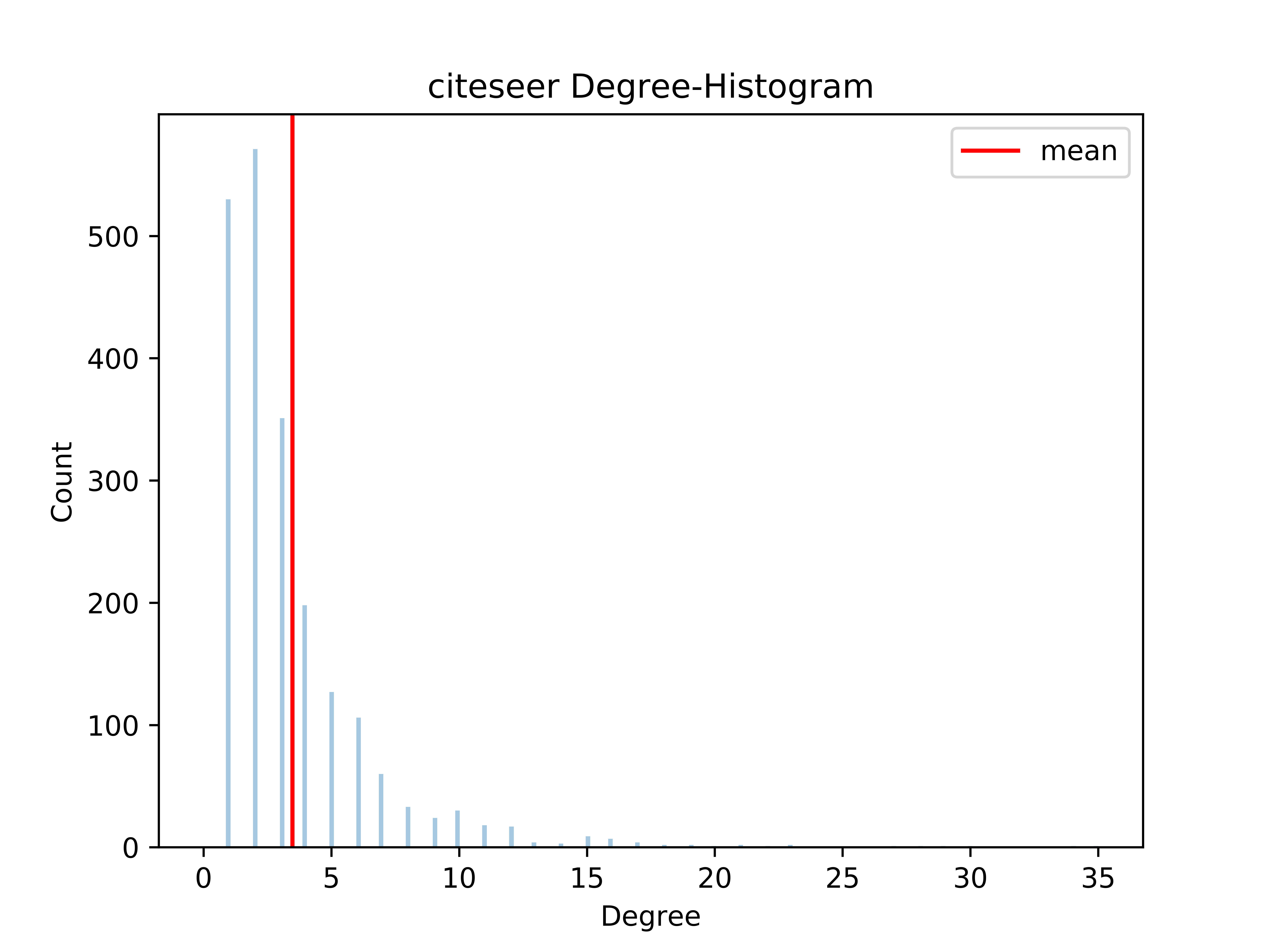
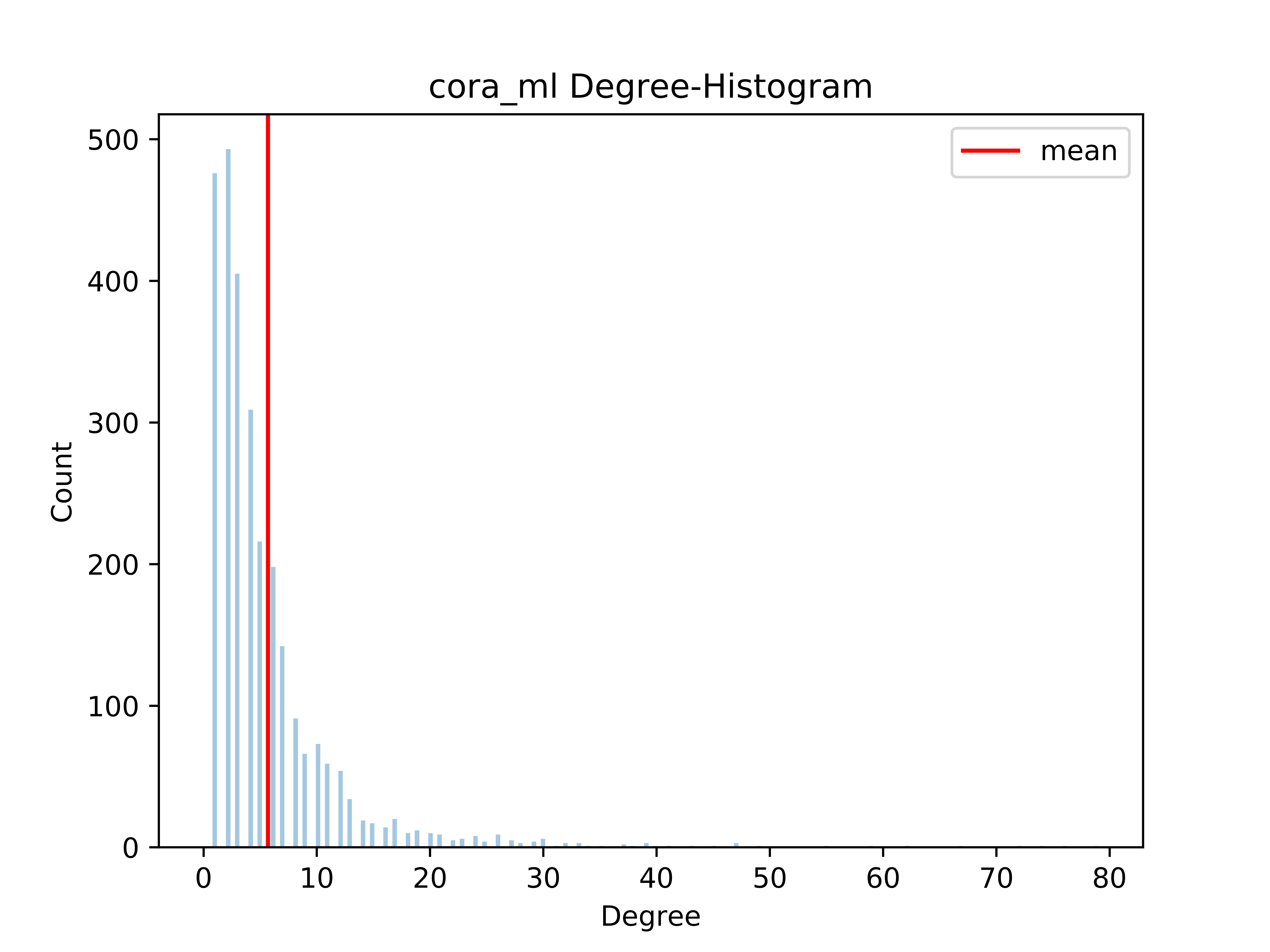
Refer to caption
Refer to caption
Refer to caption
Refer to caption
Figure 8: Histogram of node degrees

Appendix E Additional Experiments

To study the differentiability of the derived interpolation empirically, we embedded a small tree into 𝔰𝔱κd𝔰subscriptsuperscript𝔱𝑑𝜅\mathfrak{st}^{d}_{\kappa} for κ[5,5]𝜅55\kappa\in[-5,5]. To that end, we used 200200200 equidistant values κ𝜅\kappa in [5,5]55[-5,5] and trained a κ𝜅\kappa-GCN (with non-trainable curvature) to produce an embedding that minimizes distortion. Moreover we also trained a Euclidean GCN with the same architecture. The results are summarized in Figure 9.
One can observe the smooth transition between the different geometries. As expected, the distortion improves for increased hyperbolicity and worsens when the embedding space becomes more spherical. The small kink for the spherical model is due to numerical issues.

Appendix F More Experimental Details
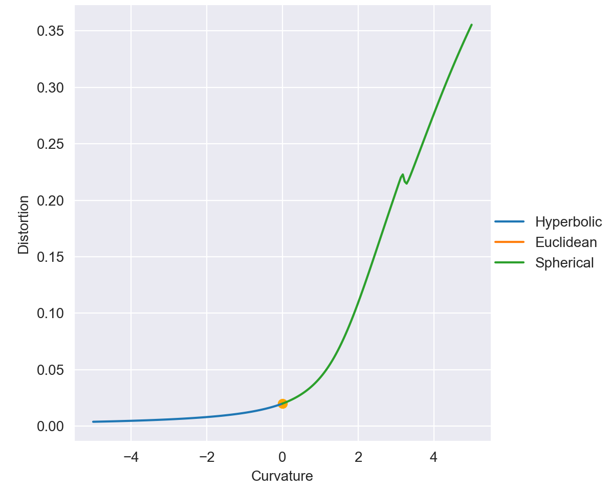
Refer to caption
Figure 9: Distortion of κ𝜅\kappa-GCNs of varying curvature κ𝜅\kappa trained to embed a tree
Algorithm 1 Curvature Estimation
  Input: Graph G𝐺G, nitersubscript𝑛𝑖𝑡𝑒𝑟n_{iter}
  for mG𝑚𝐺m\in G  do
     for i=1𝑖1i=1 to nitersubscript𝑛𝑖𝑡𝑒𝑟n_{iter} do
        b,c𝒰(𝒩(m))similar-to𝑏𝑐𝒰𝒩𝑚b,c\sim\mathcal{U}(\mathcal{N}(m)) and a𝒰(G)similar-to𝑎𝒰𝐺a\sim\mathcal{U}(G) such that ma𝑚𝑎m\not=a
        ψ(m;b,c;a)=dG(a,m)2+dG2(b,c)8dG(a,m)𝜓𝑚𝑏𝑐𝑎subscript𝑑𝐺𝑎𝑚2superscriptsubscript𝑑𝐺2𝑏𝑐8subscript𝑑𝐺𝑎𝑚\psi(m;b,c;a)=\frac{d_{G}(a,m)}{2}+\frac{d_{G}^{2}(b,c)}{8d_{G}(a,m)}2dG2(a,b)+2dG2(a,c)4dG(a,m)2superscriptsubscript𝑑𝐺2𝑎𝑏2superscriptsubscript𝑑𝐺2𝑎𝑐4subscript𝑑𝐺𝑎𝑚\hskip 68.28644pt-\frac{2d_{G}^{2}(a,b)+2d_{G}^{2}(a,c)}{4d_{G}(a,m)}
     end for
     ψ(m)=AVERAGE(ψ(m;a,b;c))𝜓𝑚AVERAGE𝜓𝑚𝑎𝑏𝑐\psi(m)=\text{AVERAGE}(\psi(m;a,b;c))
  end for
  return: κ=AVERAGE(ψ(m))𝜅AVERAGE𝜓𝑚\kappa=\text{AVERAGE}(\psi(m))

We here present training details for the node classification experiments.

We split the data into training, early stopping, validation and test set. Namely we first split the dataset into a known subset of size nknownsubscript𝑛𝑘𝑛𝑜𝑤𝑛n_{known} and an unknown subset consisting of the rest of the nodes. For all the graphs we use nknown=1500subscript𝑛𝑘𝑛𝑜𝑤𝑛1500n_{known}=1500 except for the airport dataset, where we follow the setup of Chami et al. (2019) and use nknown=2700subscript𝑛𝑘𝑛𝑜𝑤𝑛2700n_{known}=2700. For the citation graphs, the known subset is further split into a training set consisting of 202020 data points per label, an early stopping set of size 500500500 and a validation set of the remaining nodes. For airport, we separate the known subset into 210021002100 training nodes, 300300300 validation nodes and 300300300 early stopping nodes. Notice that the whole structure of the graph and all the node features are used in an unsupervised fashion since the embedding of a training node might for instance depend on the embedding of a node from the validation set. But when calculating the loss, we only provide supervision with the training data.
The unknown subset serves as the test data and is only used for the final evaluation of the model. Hyperparameter-tuning is performed on the validation set. We further use early stopping in all the experiments. We stop training as soon as the early stopping cross entropy loss has not decreased in the last npatience=200subscript𝑛𝑝𝑎𝑡𝑖𝑒𝑛𝑐𝑒200n_{patience}=200 epochs or as soon as we have reached nmax=2000subscript𝑛𝑚𝑎𝑥2000n_{max}=2000 epochs. The model chosen is the one with the highest accuracy score on the early stopping set. For the final evaluation we test the model on five different data splits and two runs each and report mean accuracy and bootstrapped confidence intervals. We use the described setup for both the Euclidean and non-Euclidean models to ensure a fair comparison.

Learned curvatures

. We report the learnt curvatures for node classification in tab. 3

Appendix G Graph Curvature Estimation Algorithm

We used the procedure outlined in Algorithm 1 to estimate the curvature of a dataset developed by Gu et al. (2019).