Evidence of dust grain evolution from extinction mapping in the IC 63 photodissociation region111Based on observations made with the NASA/ESA Hubble Space Telescope, obtained at the Space Telescope Science Institute, which is operated by the Association of Universities for Research in Astronomy, Inc., under NASA contract NAS5-26555. These observations are associated with program GO-14186.
Abstract
Photodissociation regions (PDRs) are parts of the ISM consisting of predominantly neutral gas, located at the interface between H ii regions and molecular clouds. The physical conditions within these regions show variations on very short spatial scales, and therefore PDRs constitute ideal laboratories for investigating the properties and evolution of dust grains. We have mapped IC 63 at high resolution from the UV to the NIR , using the Hubble Space Telescope WFC3. Using a Bayesian SED fitting tool, we simultaneously derive a set of stellar (, , distance) and extinction (, ) parameters for 520 background stars. We present maps of and with a resolution of 25 arcsec based on these results. The extinction properties vary across the PDR, with values for between 0.5 and 1.4 mag, and a decreasing trend in , going from 3.7 at the front of the nebula to values as low as 2.5 further in. This provides evidence for evolution of the dust optical properties. We fit two modified blackbodies to the FIR SED, obtained by combining the map with data from Spitzer and Herschel. We derive temperatures (30 K and 227 K) and the ratio of opacities at to V band ( and ) for the two dust populations. Similar fits to individual pixels show spatial variations of . The analysis of our HST data, combined with these Spitzer and Herschel data, provides the first view of dust within a PDR.
tablenum \restoresymbolSIXtablenum \turnoffeditone\turnoffedittwo
1 Introduction
Photodissociation regions (PDRs) are regions of the interstellar medium (ISM) where the physical properties of the gas are mainly determined by the radiation field of nearby O or B stars. They form a boundary layer between ionized (Hii) regions, and the rest of the molecular cloud where they reside. The FUV radiation from ionizing stars is quickly attenuated by the opacity of the relatively high density medium shielding the rest of the gas . As a consequence, there are typically sharp transitions between different regimes (e.g. Hii, Hi and H2), resulting in a layered structure (1997ARA&A..35..179H; 1999RvMP...71..173H). This makes PDRs the perfect laboratory for studying the evolution of the ISM, including the dust over different physical and excitation conditions.
Interstellar dust grains make a very significant contribution to the total opacity of the interstellar medium, and modify any radiation field through the effects of absorption, scattering and re-emission (2003ARA&A..41..241D; 2013ARA&A..51...63S). Aside from attenuating the UV radiation field that regulates the physics inside a PDR, they also couple to the gas through other processes. Dust grains play a major role in the formation of H2, through reactions that take place on grain surfaces (1971ApJ...163..155H; 2017MolAs...9....1W). They provide a major contribution to the heating of the gas through the photoelectric effect, but can also have a cooling effect when gas-grain collision occur (1994ApJ...427..822B; 2001ApJS..134..263W).
To model these effects, knowledge about the composition and size distribution of the dust grains is necessary. While there are many dust models that can explain the observed extinction curves and emission spectra , it remains difficult to accurately constrain the exact properties of the grains. Moreover, the effects of dust evolution processes can change these properties depending on the time and the environment. Some models, such as THEMIS (2017A&A...602A..46J), have built-in ways to follow the changes in dust properties. Providing better constraints on these models is crucial for understanding not only the dust itself, but also the structure and evolution of PDRs and the ISM in general.
Evidence for dust evolution in PDRs has been found through observations in the mid and far-infrared.
A comprehensive study of the physics and chemistry of IC 63 can be found in 1994A&A...282..605J; 1995A&A...302..223J; 1996A&A...309..899J. A study using Infrared Space Observatory (ISO) data has characterized the fine structure and H2 lines in IC 63 (2009MNRAS.400..622T), and the distribution of Polycyclic Aromatic Hydrocarbons (PAHs) has been derived from Spitzer data (2010ApJ...725..159F). Recently, Herschel FIR maps and FIR spectroscopy data were combined with [C ii] 157 velocity maps from the GREAT instrument on board the SOFIA observatory to revisit IC 63 in greater detail (2018A&A...619A.170A).
In this work we aim to study the spatial variations of the dust properties observed through extinction, in particular through the and parameters (1989ApJ...345..245C). IC 63 is a most suitable target for this, as it has many observable background stars, each of which provides information about the medium along a specific line of sight. Grouping these stars into spatial bins makes it possible to measure the average extinction for a number of regions on the sky. To measure the extinction for each star, we use the same approach as in 2016ApJ...826..104G for the Panchromatic Hubble Andromeda Treasury (PHAT) survey data (2012ApJS..200...18D). A catalog of point sources is generated from broadband Hubble Space Telescope (HST) observations, to which our Bayesian Extinction And Stellar fitting Tool (BEAST, 2016ApJ...826..104G) is applied.
In section 2, we describe our 7-band photometric observations with HST, and how we extract photometric measurements for 520 background sources. Our Bayesian extinction fitting tool is introduced, and some necessary modifications to it are explained. Section 3 presents the individual fit results for the sources, and how these were processed to create and maps. In section 4, we compare our findings to earlier studies of IC 63, and use data from Herschel and Spitzer combined with our maps and modified blackbody fits to derive the -normalized dust surface brightness and dust optical depth.
2 Data and Analysis
2.1 Hubble Observations
The photometric data for the various sources behind IC 63 were obtained through observations with the Wide Field Camera 3 (WFC3) of HST, using both the UVIS (UV and visual) and IR (infrared) channels. We obtained photometric images in the F275W, F336W, F475W, F625W, F814W bands with the UVIS chip, and in the F110W and F160W bands with the IR chip. This set of broadband filters was chosen cover the stellar SED from the UV to the near infrared, and to optimize the extraction of the dust extinction parameters through SED fitting. The IR measurements provide a way to resolve the degeneracy between the stellar surface temperature and the reddening, while the UV filters constrain the type of extinction. A similar observing strategy, and a more detailed reasoning for choosing each filter can be found in 2012ApJS..200...18D.
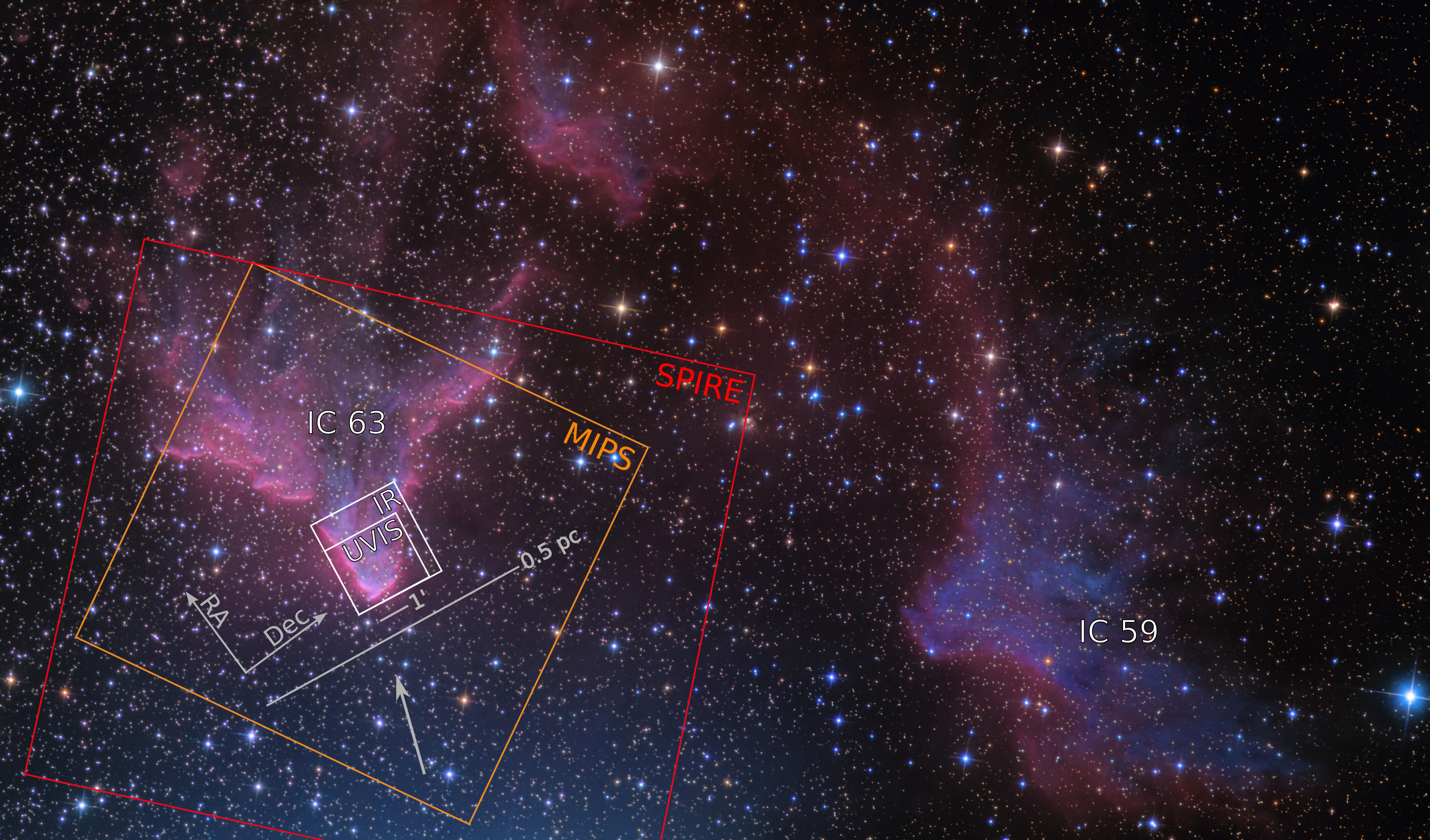
The UVIS images span a field of view (FOV) of 162 by 162 arcsec, while the FOV for the IR images is somewhat smaller, at 123 by 136 arcsec (Figure 1). The observing program consisted of two visits, each two orbits long. During the first visit , the F275W and F336W exposures were taken, followed by F814W and F160W. During the second visit , the F625W, F110W, F475W and additional F275W exposures took place. See Table 1 for the exposure times. The time difference of several days between the visits is intentional, to prevent persistence for the IR exposures.
Guard exposures for bright stars where taken for 5s in F475W and F814W between the two orbits of the first and second visit, . To help dealing with macroscopic features of the detector and cosmic rays, a gap line dither pattern was used all exposures with UVIS except the guard exposures. For the IR, a small line pattern was used instead to minimize blurring due to IR persistence. A post-flash was used for all UVIS exposures, except F625W.
The photometry described in section 2.3 works with the flt files (for IR) and flc files (for UVIS).
| channel and filter | exposure time | |
|---|---|---|
| UVIS F275W | ||
| UVIS F336W | ||
| UVIS F475W | ||
| UVIS F625W | ||
| UVIS F814W | ||
| IR F110W | ||
| IR F160W |
2.2 Ancillary Data
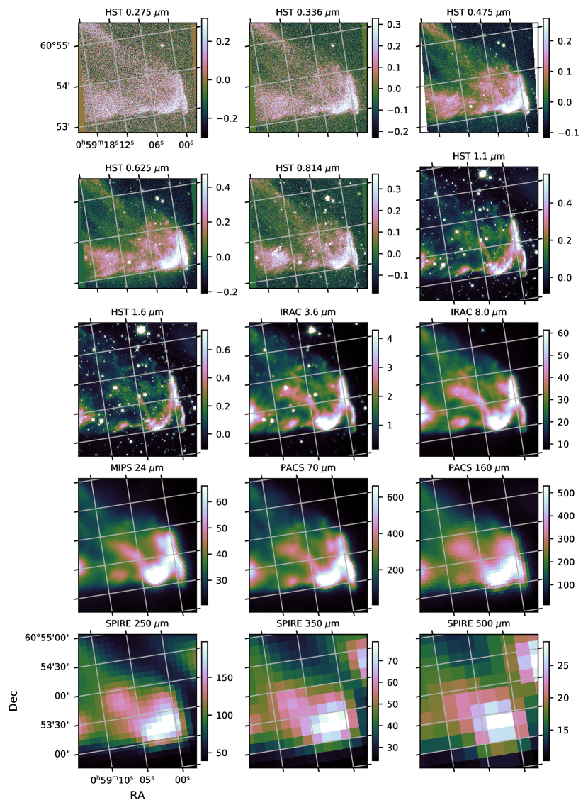
The FIR PACS (2010A&A...518L...2P) and SPIRE (2010A&A...518L...3G) imaging data were obtained from the Herschel Science Archive. They were originally part of a key program for the Herschel Space Observatory (2010A&A...518L...1P), “Evolution of Interstellar Dust” (2010A&A...518L..96A). We also retrieved IRAC (2004ApJS..154...10F) and MIPS (2004ApJS..154...25R) photometric data from the Spitzer heritage archive, taken under the “Star Formation in Bright Rimmed Clouds” program (ID 202). An overview of the images can be found in Figure 2, where these data were reprojected onto the same coordinate frame as the drizzled HST UVIS images.
2.3 Point Source Photometry
2.3.1 Source Extraction
We employ a technique analogous to the one used to extract similar photometric catalogs from the PHAT (2012ApJS..200...18D; 2014ApJS..215....9W), SMIDGE (2017ApJ...847..102Y) and METAL (2019arXiv190106027R) data. Following a precise astrometry and alignment step, the photometry software DOLPHOT (2016ascl.soft08013D) is used to automatically detect the point sources, and to determine their positions and fluxes, based on Point Spread Function (PSF) fitting. The details about this photometric extraction routine are described in 2014ApJS..215....9W. However, we do use the same tweaks as 2019arXiv190106027R. The are used instead of the Anderson libraries . have already been corrected for CTE. Therefore, a separate CTE correction step after the PSF fitting is no longer necessary.
2.3.2 Removal of Spurious Detections
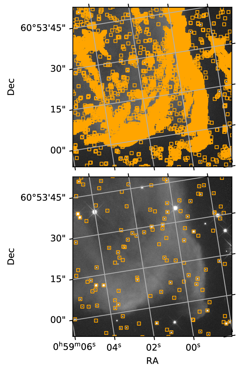
Due to the relatively bright extended emission in IC 63 (stellar light scattered by dust, gas emission lines due to recombination), the majority of the sources listed by the automatic source detection algorithm mentioned above are false positives. This can be seen in Figure 3, where most of the detections clearly coincide with the extended emission. Fortunately, we found some simple criteria to separate the bulk of these spurious detections from the real point sources, making use of some of the quantities provided by the PSF fitting routine. These quantities are given in certain columns of the photometric catalog.
The first criterion is a cut on the relative flux error in the F814W band. We only keep the sources for which the error to flux ratio . This excludes almost all of the entries due to the extended emission and some diffraction spikes of bright stars.
Secondly, an extra cut on the crowding is performed, specifically . This removes a handful of overlapping sources, as well as several remaining detections located at diffraction spikes. The thresholds for these first two cuts were obtained through some trial and error. By visually inspecting plots such as Figure 3, we found that these values remove most of the spurious detections, while keeping detections of obvious point sources intact.
Lastly, we remove all sources that are outside the region where observations exist in all bands, to provide a homogeneous dataset for analysis. The right panels of Figure 3 show the positions of the sources that are left after applying the cuts. There are 520 sources remaining, over the area covered by both the UVIS and IR chip.
2.4 Physics Model
To model the stellar SED attenuated by dust for each source, we employ the Bayesian Extinction And Stellar Tool (BEAST; 2016ApJ...826..104G). This tool works with a 7D grid of SED models, one dimension for each parameter (, , , , , , ; see description below and Table 2). For each set of parameters, the physics model makes a prediction for the observed SED of the source. This is done by first constructing models for the stellar spectrum and the extinction curve. The model spectrum is then extinguished according to this curve at each of its wavelength points, and integrated over the transmission curve of each filter.
2.4.1 Stellar Parametrization
In the current implementation, the models for the stellar spectra are calculated based on parameters, specifying the star’s birth mass , age , metallicity , and distance . Starting from the first three parameters, the luminosity of the star and the shape of the spectrum are calculated using a combination of publicly available stellar atmosphere grids (2003IAUS..210P.A20C; 2003ApJS..146..417L; 2007ApJS..169...83L) and evolutionary tracks (2008A&A...482..883M; 2010ApJ...724.1030G; 2012MNRAS.427..127B; 2013EPJWC..4303001B). The reasoning behind this choice of parameters can be found in 2016ApJ...826..104G. .
2.4.2 New BEAST Feature: Distance as an Extra Stellar Parameter
Prior to this work only a single value for the distance was supported, as this tool had only been applied in the extragalactic context where a single distance to all stellar sources can be assumed. For IC 63, setting a single distance is of course not possible, as all the background stars are located within the Galaxy, and hence they have a wide variety of distances. Therefore, in the version of the BEAST used for this work, the distance was implemented as an extra parameter for the stellar model.
2.4.3 Extinction Parametrization
The other parameters describe the shape and magnitude of the extinction curve. The BEAST features a two-component dust extinction model, mixing two different shapes (wavelength dependencies); the type- curve, which models the average extinction as measured in the Milky Way (MW), and the type- curve, which models that of the Small Magellanic Cloud (SMC) Bar (2003ApJ...594..279G). For the MW-like type, the shape of the extinction curve depends on
| (1) |
where is the total Johnson V-band extinction by the dust, and . This dependence is modeled according to 1999PASP..111...63F. The SMC-like extinction model does not depend on , and its wavelength dependence is modeled using an average of the measurements given by 2003ApJ...594..279G. Within this model, the value of is a way to express the total dust column, while A third parameter, , takes a linear combination of shapes and :
| (2) |
This extinction model is then applied to the stellar spectra generated from the first four parameters.
2.4.4 Model Details for This Work
The details about the parameter ranges and their spacing in the BEAST physics model grid are summarized in Table 2. Suitable ranges and resolutions were obtained through a combination of previous experience (such as Table 1 in 2016ApJ...826..104G), some trial and error, and some compromises considering computational resources.
The parameters shown in the table give rise to about models, and without compression, about 1.6 TB of disk space is needed to store this grid. The resolution for most of the parameters is relatively low, because a relatively large range and number of bins is needed for the distance.
| Parameter | Description | Min | Max | Resolution | Prior |
|---|---|---|---|---|---|
| (years) | stellar age | 6.0 | 10.13 | 0.3 | constant SFR |
| () | stellar mass | -1.0 | 2.5 | variableaaSupplied by isochrone model grid | Kroupa IMF |
| (mass fraction) | stellar metallicity | -3 | -1.2 | 0.15 | flat in |
| (pc) | distance | 2.7 | 4.2 | 0.037bbThis corresponds to 40 logarithmic steps from 500 to 15000 pc | flat in |
| (mag) | dust column | 0 | 10.05 | 0.08 | flat |
| dust average grain size | 1.5 | 5.5 | 0.5 | flat | |
| dust mixing parameter | 0 | 1 | 0.2 | flat |
The priors are shown in the rightmost column of Table 2. For the new distance parameter, the prior is chosen to be flat as a function of . As a consequence, for some stars a degeneracy exists between the estimated distance and mass (or luminosity): an observed star can either be far away and of a luminous type, or nearby and of a fainter type. The multi-band photometry partly resolves this degeneracy, and we did not find this effect to be problematic for constraining the extinction.
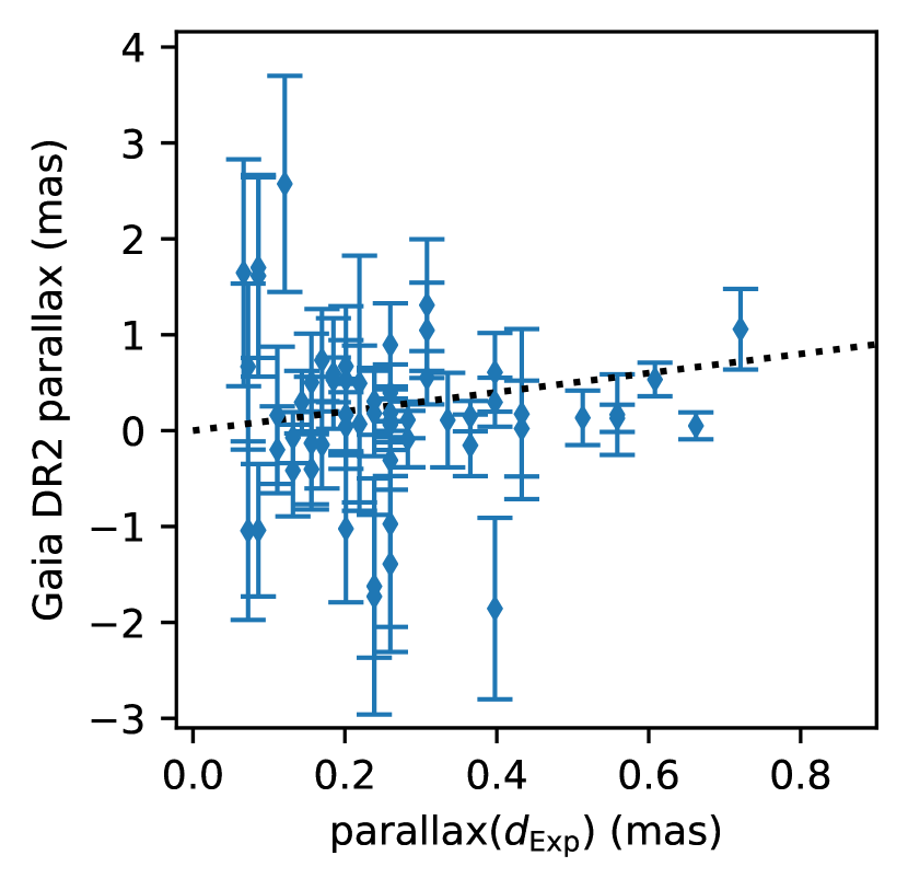
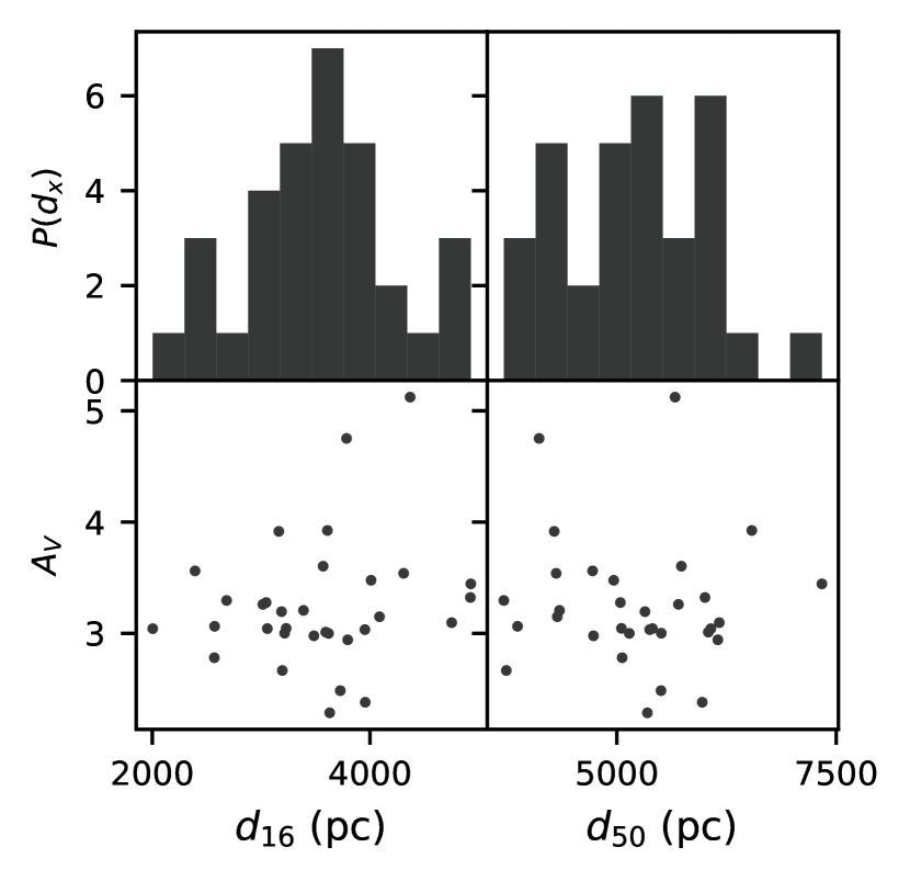
In the future, more physically motivated priors could be implemented for the distance, such as an exponentially decreasing space density (Bailer-Jones2018). Another option would be to make direct use of the parallaxes provided by Gaia DR2 (2016A&A...595A...1G; Gaia-Collaboration2018; Luri2018), and use them as source-specific priors in a post processing step. However, since there are only 59 out of 500 stars in our data set with Gaia data available, this would have a limited impact on the results of this work. Moreover, we did cross check the Gaia data with our fit results, and found that the parallaxes derived from the distances were consistent with the fairly uncertain Gaia parallaxes (Figure 4)
2.5 Noise Model
2.5.1 Artificial Star Tests
By applying the physics model to all combinations of the parameters, a grid of theoretical SEDs is constructed, representing the observations in the relevant filters under perfect circumstances. But in a realistic setting, when the flux is measured from imaging data, the flux values that are extracted for a certain point source are not only affected by shot (Poisson) noise and the PSF, but also by nearby objects, various sources of background, instrumental artifacts, and the extraction algorithm itself. Nearby point sources can create crowding effects (2016ApJ...826..104G), which increase the noise and cause an overestimation of the flux. However, since the density of observed stars in IC 63 is very low compared to the size of the PSF, these effects are negligible. For IC 63, the main expected contributor to the observation model is the presence of a foreground and background of extended emission, such as H emission of the gas or stellar light by dust grains.
To quantify how significantly one of the model SEDs differs from the observed SED of a certain star, we create a model describing the uncertainty (error ) and systematic deviation (bias ) for each flux. While the photometric catalog produced by the PSF fitting does contain values for the uncertainty on each flux (which we used to perform the input cleaning step), these do not cover all possible error sources. Instead, we treat the errors as a property of each theoretical model: for each grid point , we aim to calculate the error or uncertainty and a bias in every band.
The starting point for this calculation is a set of Artificial Star Tests (ASTs). The input for a single AST consists of a theoretical SED and a position. These parameters are used as input for the fake star mode of DOLPHOT. This routine will insert a fake star with the given SED into each of our observations, simulate the PSF and photon noise, and then perform the exact same photometric extraction routine. The result is a set of output fluxes, representing a mock-observation of a point source with that specific theoretical SED. By putting the same source at many different positions, statistical information is obtained about the deviations that occur when observing that specific SED , from which appropriate values for and can be derived.
Ideally, such a set of tests would be performed for each SED in the physics grid, leading to an individual measurement of the noise for each model. However, performing a single AST takes about 2 minutes of computing time on a modern processor, so doing this for the billions of models contained in the physics grid is practically impossible. Therefore, it is customary to produce a sample of SEDs that is representative of all the models relevant for fitting the observed sources.
2.5.2 New BEAST Feature: Uniform SED Sampling by Magnitude
Since the distance parameter can strongly scale the model SEDs, faint stars at long distances and luminous stars at short distances will have model fluxes that are far away from the minimum and maximum of the observed catalog. Their noise parameters are not useful for fitting our observed SEDs. Therefore we only consider models that have fluxes that fall between the minimum and maximum of the observed SEDs, with 1 magnitude of leeway to allow for a range of uncertainty. The magnitude ranges of the remaining models are then discretized into 25 bins for each filter, and SEDs are chosen randomly from the physics grid and added to the AST input list. For each SED that is chosen, the corresponding magnitude is determined in each band, so we can keep track of the number of ASTs that will cover each filter-mag bin. The algorithm continues until we have 50 samples in each bin, and the resulting set of AST input SEDs will have a magnitude distribution that is more or less flat in each filter.
Figure 5 shows the difference between the original method which evenly samples by stellar age, and the new method which evenly samples by magnitude. To show the magnitudes that need to be covered, the distribution of the observed catalog is also shown. The original method does not sufficiently sample the low brightness range, while simultaneously producing many samples that are several magnitudes brighter than the maximum of the observed catalog. As designed, the new method produces a certain minimum number of samples for each flux bin, within a more suitable range. The peaks that appear in the distribution depend on the contents of the physics grid and the brightness cutoffs. were picked to fill the rarer flux ranges in other filters. Note that the new method still produces many samples outside of the observed flux range, because we only require that at least 3 bands fall within that range. This allows for a larger variety of SED shapes to be picked for the ASTs.
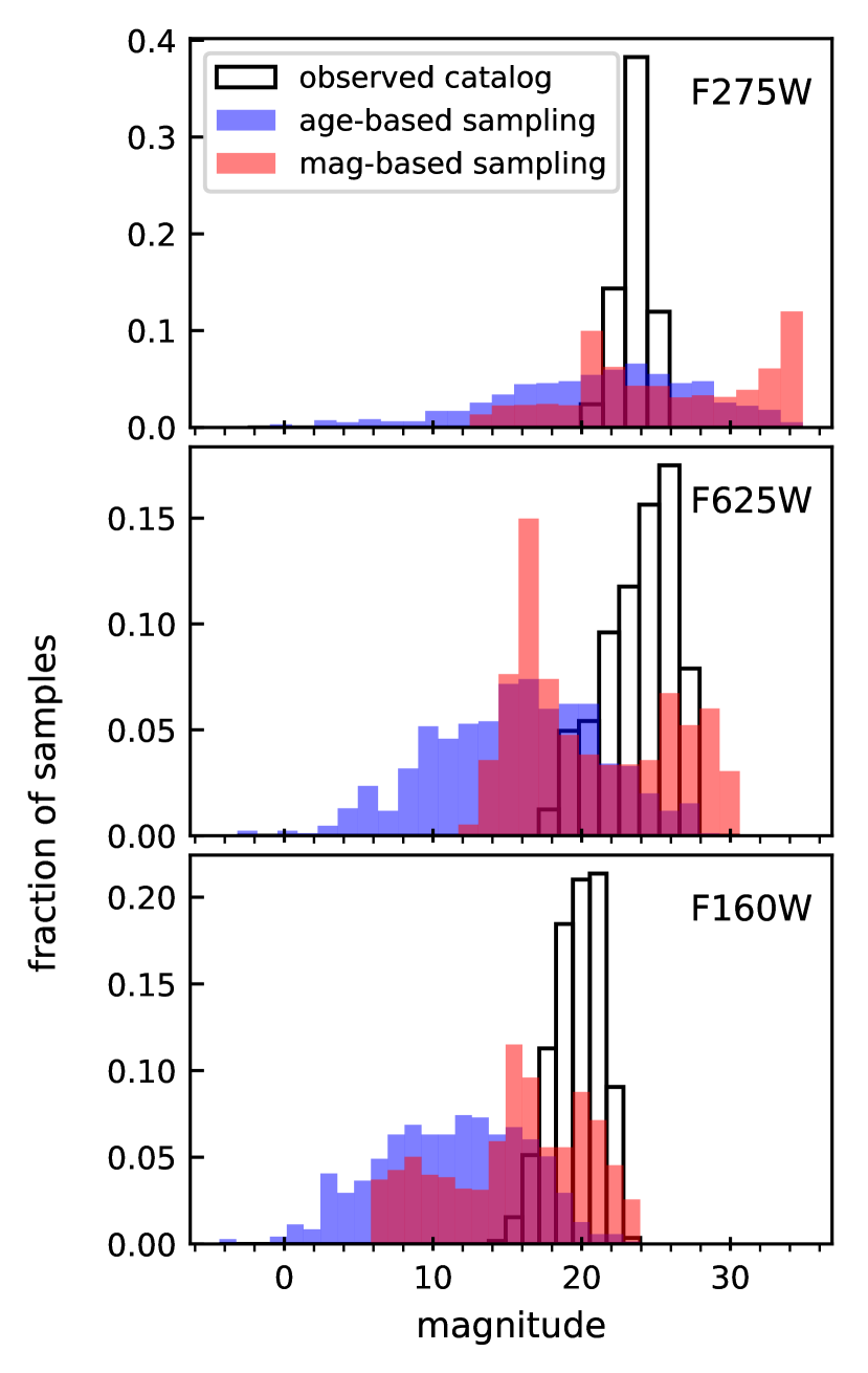
Using this approach, a list of about 2500 SEDs was generated. This list is duplicated multiple times while giving a random position to each SED, leading to 180000 unique ASTs. The list of ASTs was split up into a set of jobs, each of which have a manageable runtime. These jobs were executed across three machines with the help of GNU parallel (Tange2011a), using 78 of the available cores over the course of 3 days. The results were then merged and processed into a single fake star catalog, of the same format as the one containing the observed photometry.
2.5.3 From ASTs to Noise Model
Before the fake star catalog is further processed by the BEAST to generate the noise model, the same selection function used in section 2.3.2 is applied. This way it is ensured that the observation model generates a set of noise parameters that is representative of our cleaned ensemble of observed stars. Note that this also removes ASTs which are missing a flux in one or more bands, which includes those positioned outside the IR chip’s FOV. After this step, about 80000 fake stars remain.
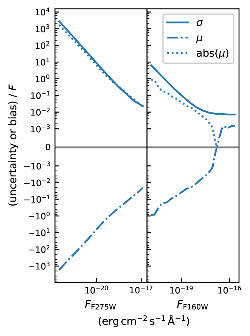
To generate the noise model for each SED in the physics grid, the BEAST’s most conservative method is used, which considers each flux individually and as such ignores any correlations between the bands. This method minimizes the number of ASTs needed, which is already quite large due the broad range of fluxes needed to model all the distances. Similarly to how the AST input SEDs were chosen, the flux ranges of the model SEDs are divided into 30 bins. For each bin, the input and output SEDs of the relevant ASTs are compared, producing statistical values for the error and the bias in that flux range, for a specific filter. By interpolating between these bin-averaged values, each filter now has a model that predicts and as a function of the theoretical flux . This behavior is shown in Figure 6.
One of the main features of the noise model is that the bias seems to be negative for all but the brightest fluxes, in all bands. This means that the fluxes extracted by the photometry routine are on average smaller than the input fluxes of the fake stars.
For weak fluxes, the constant slope of the relative and implies that the noise parameters are dominated by photon noise and/or constant features in the image. For stronger fluxes, the relative error levels off while the bias becomes positive (but much smaller than the error). This means that fractional deviations dominate instead, which are most likely caused by the PSF or imperfections in the photometry routine. For all bands except the UV band, the absolute value of seems to be smaller than . This means that the exact value of will have less of an effect on the results, as it only causes deviations within .
Since we suspect that the background/foreground extended emission provides the main contribution to the noise model, we experimented with a noise model that is stratified according to the intensity of this emission. In the appendix, we explain how we determine 4 regions of similar background/foreground intensity, and create a separate noise model for each of them. Ultimately, the fitting results obtained using these individual noise models were not found to be significantly different, so the rest of the analysis was performed using the single noise model presented in this section. However, these tools integrate well with and improve upon existing code that deals with varying levels of crowding, and have therefore been incorporated in the main BEAST branch.
2.6 Fitting Procedure and Output
Once the necessary models have been set up, the fitting step comes down to calculating a 7D posterior probability distribution
| (3) |
for each of the observed point sources. Here, is the observed SED, and and represent the SED and the noise parameters for one of the models, evaluated at a specific point of the 7D parameter grid. . The grid point at the global maximum of distribution is considered to be the best fitting model. The likelihood function is a 7D multivariate Gaussian:
| (4) | |||
| (5) | |||
| (6) |
In principle, the whole 7D log-likelihood can be written to disk for each star. In practice, only a local area around the peak of the posterior distribution is written out. Additionally, the 1D marginal probability distributions for each parameter are also available. For our purposes however, some statistics derived from the posterior are sufficient. For all the parameters, the best fit, the expectation values, and the 16th, 50th and 84 percentiles are calculated and stored in a table that contains one row per source. The of the least-squares model and of the best fitting model are also stored. The former gives us some insight about the quality of the grid and the noise model, and the source itself. A high usually means that the grid range or resolution is not sufficient, that there might be something wrong with the noise model, or that a source in particular has an SED that is very much unlike that of an extinguished star.
3 Results
3.1 Postprocessing
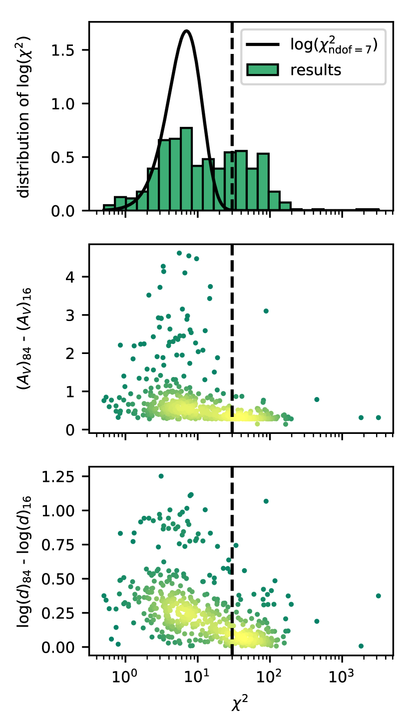
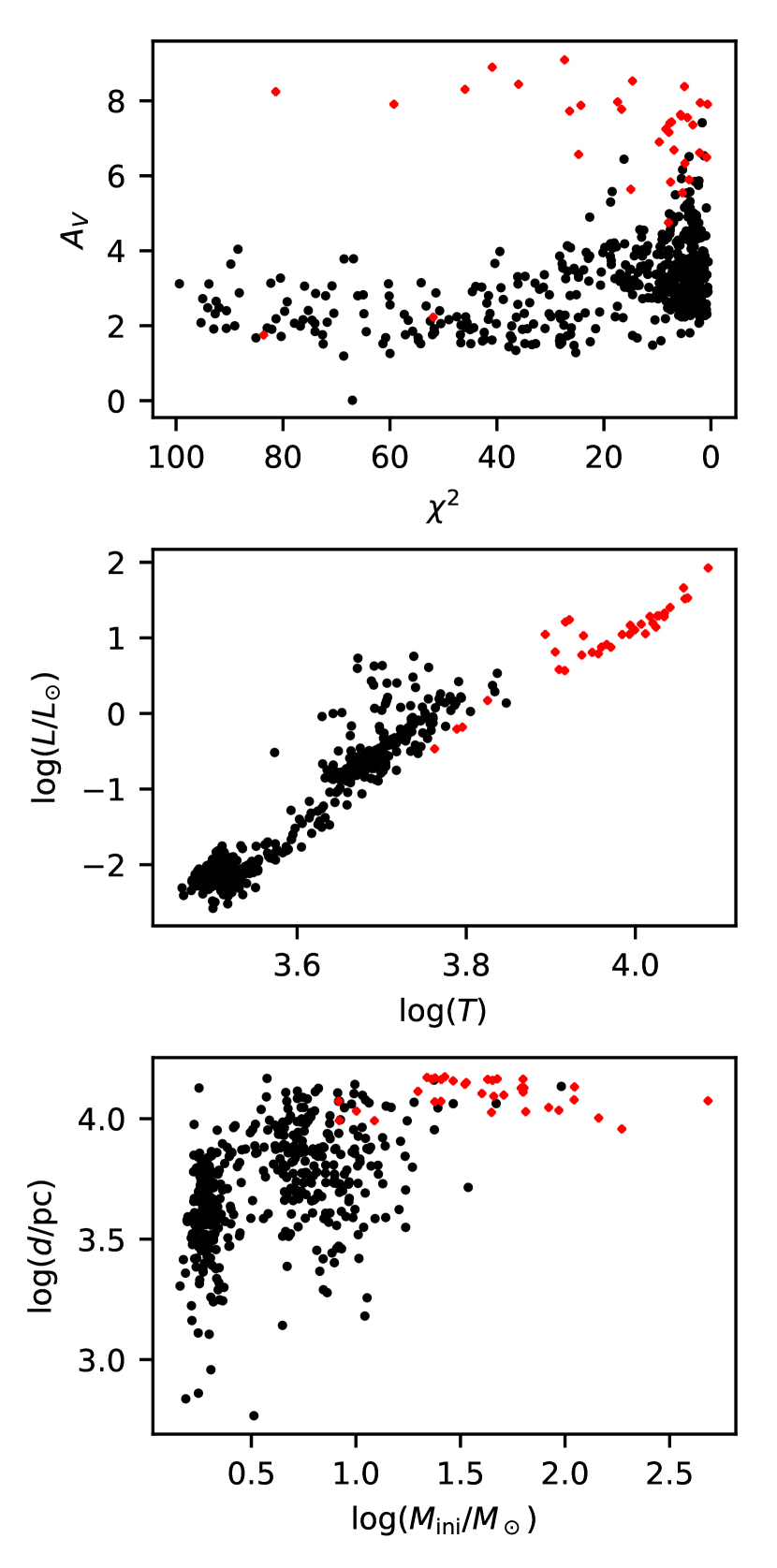
Following the workflow described in the previous section, we obtained a catalog for all 520 sources (Figure 3) that were left after applying the criteria from section 2.3.2. This catalog contains statistics for the seven main parameters, as well as a set of derived stellar quantities: current mass , radius , luminosity , surface gravity , temperature and magnitude . The distribution of the expectation values of the seven parameters and the correlations between them are shown in Figure 7, and the distribution is shown in Figure 8. The latter seems to be slightly peaked around 7, which could naively be attributed to the fact that we have measurements in bands. But in practice, the distribution of this is not as simple to interpret, because there are significant correlations between the observed fluxes in different bands. The value can only be used as a rough check that the fits are reasonable.
The two bottom panels of 8 show that for almost all sources with a higher (30 to 200), the width of their 1D posterior and distance distribution is near the minimum cutoff. This means that the resulting fits are acceptable despite their high values; their accuracy is simply limited by the resolution of the grid. Decreasing the and distance spacing will likely improve the and make the distributions narrower, but we consider the precision achieved with the current parameters sufficient for the analysis that follows. Since the distance is a nuisance parameter which is integrated over to obtain the and expectation values, increasing the distance resolution will arguably have a negligible effect.
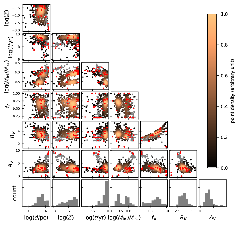
Based on the corner plot of Figure 7, there seem to be no correlations or degeneracies It is however remarkable that the population of stars seems to have a bimodal distribution of the fitted initial mass . Figure 9 shows a color magnitude diagram, and it can be seen that the seem to have a gap along the color axis.
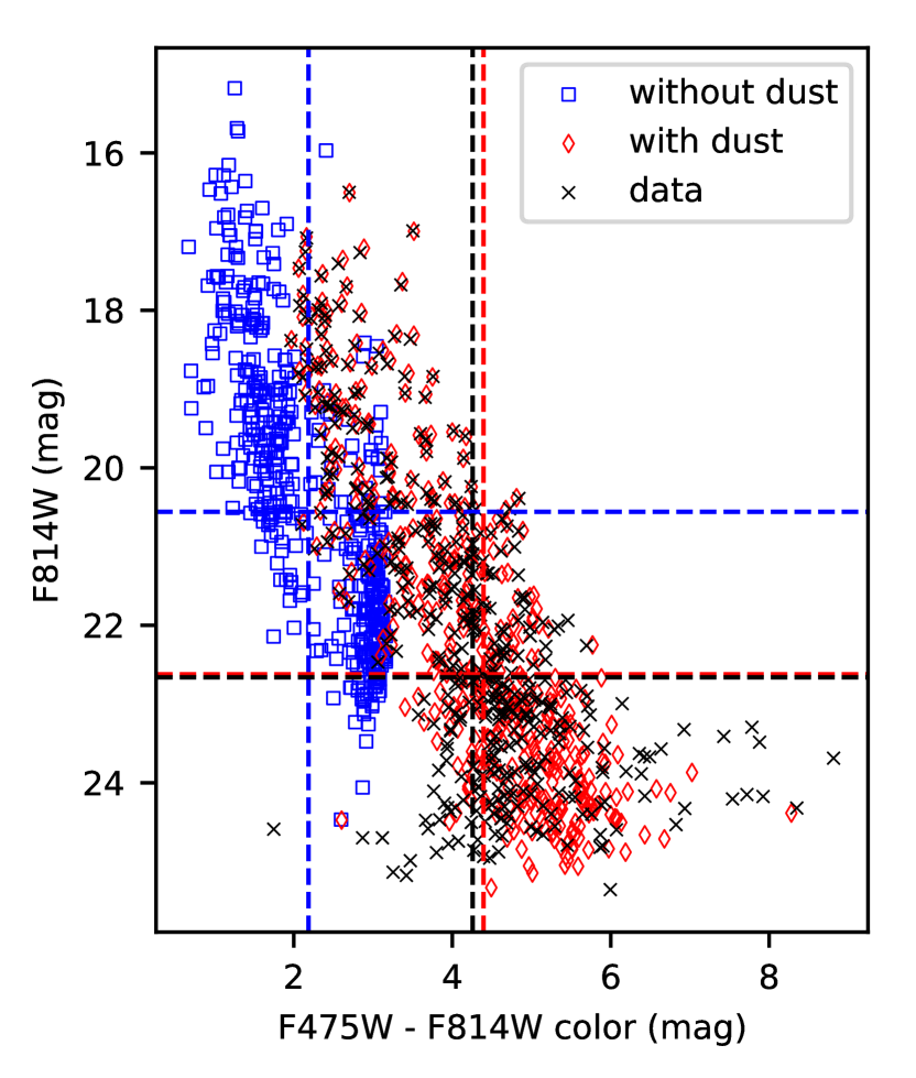
We perform a second cleaning step, which removes sources from the output catalog for which the obtained parameters are likely to be incorrect. For certain sources, the shape of the observed SED does simply not resemble that of a star with a certain extinction. The reason for this can be physical, because it’s a type of star not covered by the BEAST model, or because there is some other phenomenon at play which is not common enough across the image to be captured by the noise model (e.g. unusually strong scattered light, background galaxy, diffraction spikes). Most of these are easy to spot, with usually being several hundreds or thousands. Based on the histogram shown in Figure 8, we apply a cutoff of to remove the worst offenders.
There also seems to be group of stars for which the is not necessarily large, yet their is unusually high ( mag). When inspecting the other parameters for these stars (Figure 10), they all seem to have high temperatures (), luminosities (), masses (, and distances (). This likely points to a type of star which the BEAST fails to fit correctly, due to the necessary stellar models not being present. The resulting parameters might provide an acceptable SED, but their values are likely unphysical. In the second panel of Figure 10, a gap can be seen at a temperature of . We choose to place a cut on the temperature there; all stars that have an expectation value or best fit value of are deemed suspicious, and are removed from the catalog.
This phenomenon has some similarities with a previously documented failure case for the BEAST, which occurs when an attempt is made to fit the SED model to a Thermally Pulsing Asymptotic Giant Branch (TP-AGB) star222https://beast.readthedocs.io/en/latest/beast_issues.html.
3.2 and Maps
The main objective of this work is to look for signs of dust evolution, by mapping the spatial variations of the and parameters. The maps, shown in Figure 12, are constructed by creating a rectangular grid, aligned with the right ascension and declination axes. The angular size of each map pixel is roughly 25 arcsec, which provides us with about 10 to 20 sources per (except at the edges, as indicated with a green on the figure). The and values are calculated by considering all the that fall within their boundaries, and taking the median of the expectation values. Some of the have no sources in them at all, mainly due to geometry effects, as the does not line up with the edges of the IR data. These are indicated with a red X. The error for each is estimated by computing the standard deviation for the same set of values, and dividing it by the square root of the number of sources . The typical error is mag for , and for .
To highlight the variations of () across the nebula, some contours are shown which have been calculated directly from the maps. The contour levels for the maps were chosen by taking 4 linearly spaced values between the 16th and 84th percentiles of the total range of () values. The same contours are plotted onto the SPIRE 350 micron image, to indicate the spatial correspondence between features of the and maps and those of the FIR emission.
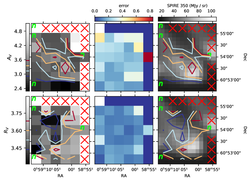
It should be noted that does not drop to zero outside of the visible gas of the nebula. In the area at the bottom of the map, just outside the visible edge of the gas, an is still observed while the 350 micron emission reaches a minimum (near the background level of MJy / sr). A selection of 50 stars in this area, has an distribution centered at 2.5 mag, with a spread of 0.70 mag. They have a mean of , and we assume that this is the extinction produced by material in the background (or foreground) of IC 63.
4 Discussion
4.1
The map shows that the extinction peaks at Given the background estimate of the previous section, the average amount of extinction added by the tip of IC 63 is hence
| (7) |
The higher values seem to lie along a ridge-like feature containing this maximum, more or less parallel to the direction of the radiation . The of this part in the nebula typically ranges from 1.0 to 1.4 mag. With the exception of the bottom row of the map which we used to measure the background, we find a minimum of 3.0 mag, or a of at least 0.5 mag for the rest of the values.
In the top right of the map, a feature with a much higher can be seen, 2.5 mag when subtracting the background. On the full version of the SPIRE map, feature is a bright part of a larger structure in the FIR, which does not have optical emission. In the NIR , it can be seen very faintly. We do not consider this structure part of the PDR, and we ignore its contribution in the analysis that follows.
4.2
The measurements over individual stars have a spread of 0.5, and a mean of (the error on the mean is this small due to the number of sources in our sample, but excludes systematics). The contours in Figure 12 seem to indicate a slight drop in , going from at the front, to at the back of the PDR.
One also has to take into account that the observed is a mix of that of the nebula and the background. Since the of the background ( mag) is larger than that of the nebula (0.5 to 1.4 mag), the drop in of the dust in IC 63 will be stronger than what is observed. We can write the measured in terms of the extinction parameters of the two parts: , for the background, and , for the nebula
| (8) |
where we use the fact that the measured is sum of the two contributions. Isolating from this equation, we obtain
| (9) |
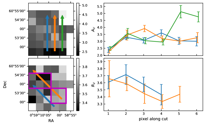
Knowing and from our maps, and using our value of mag obtained earlier, we just need to assume a value for . It should be noted however that equation 9 is quite sensitive to the assumed value of . For example, picking a value near the Galactic average of often leads to very high or even negative values for . If we take the average over the same region that we used to determine , we obtain .
The galactic map by 2017ApJ...838...36S shows values between 3.0 and 3.7, with variations at kiloparsec scales. While there might still be variations at smaller scales, we assume that and stay constant over our field of view. With these assumptions, we find that ranges from 3.7 at the bottom right of the map (tip of the nebula), to values between 2.5 and 3.3 near the top left. Since correlates with the average grain size, this points to the existence of processes making the average grain size of the dust population larger at the front of the nebula. Possible candidates are coagulation and accretion at the tip of the nebula due to higher gas densities (2003A&A...398..551S; 2015A&A...579A..15K).
2013ApJ...775...84A determined and for 14 observed background stars of IC 63. This was done using a spectral classification of the stars, followed by a calculation of using the relation (1999PASP..111...63F). Via the total-to-selective extinction and the color excess , was then obtained. Unfortunately these stars are not present in our sample, as they were either too bright (and removed per section 2.3.2), or simply outside of the field of view. They obtained an average value , which is significantly lower than the values listed by our map.
4.3 Column Density to Ratio
Our results have an average across IC 63 of 3.3 mag, or 0.8 mag with the background subtracted. As a check on the validity of this measurement, we make an estimate of the to ratio.
The relationship between the extinction and the column density of hydrogen has been found to be linear, on average in the Milky Way. Different values for the ratio have been found, by using far-UV extinction observations (1978ApJ...224..132B; 1994ApJ...427..274D) and observations of X-ray sources (1973A&A....26..257R; 1975ApJ...198...95G; 1995A&A...293..889P; 2009MNRAS.400.2050G). The most recent measurements by 2017MNRAS.471.3494Z show that is more or less invariant across the Galaxy, and .
The HI4PI 21 cm survey (2016A&A...594A.116H) . Since we can not distinguish the 21 cm contribution of IC 63 from that of the background, we assume that the ratio is the same for IC 63 and its background, and we divide by .
| (10) |
2018A&A...619A.170A used H2 excitation diagrams based on IRS spectra from Spitzer to determine the gas temperature and column density for the molecular component. They found that it consists of two components, of which the cooler one has a temperature of and a column density of while the warm component has and . Given the dominant (cold component) value from 2018A&A...619A.170A for the column density of H2, and our background subtracted value for the average , we find a ratio of
| (11) |
The combined value is
| (12) |
This value is quite close to the value from the literature mentioned above. Looking for a separate velocity component in the Hi data, and combining our measurements with better MIR spectroscopy, would provide a way to the molecular fraction and the gas to dust ratio for IC 63.
4.4 to Surface Brightness Relation
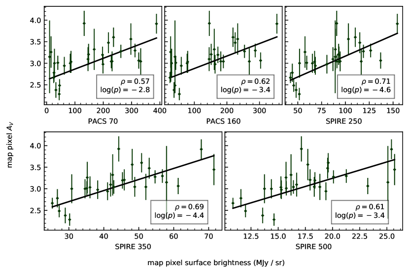
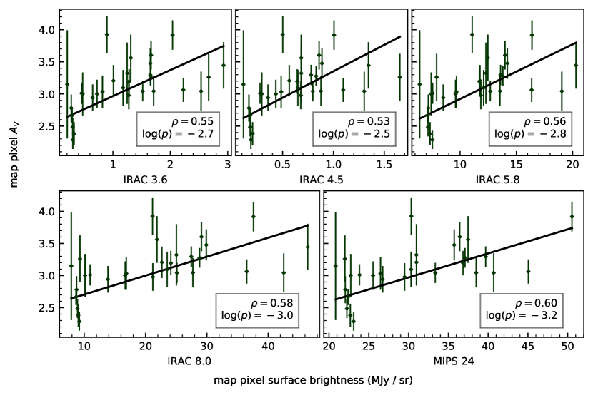
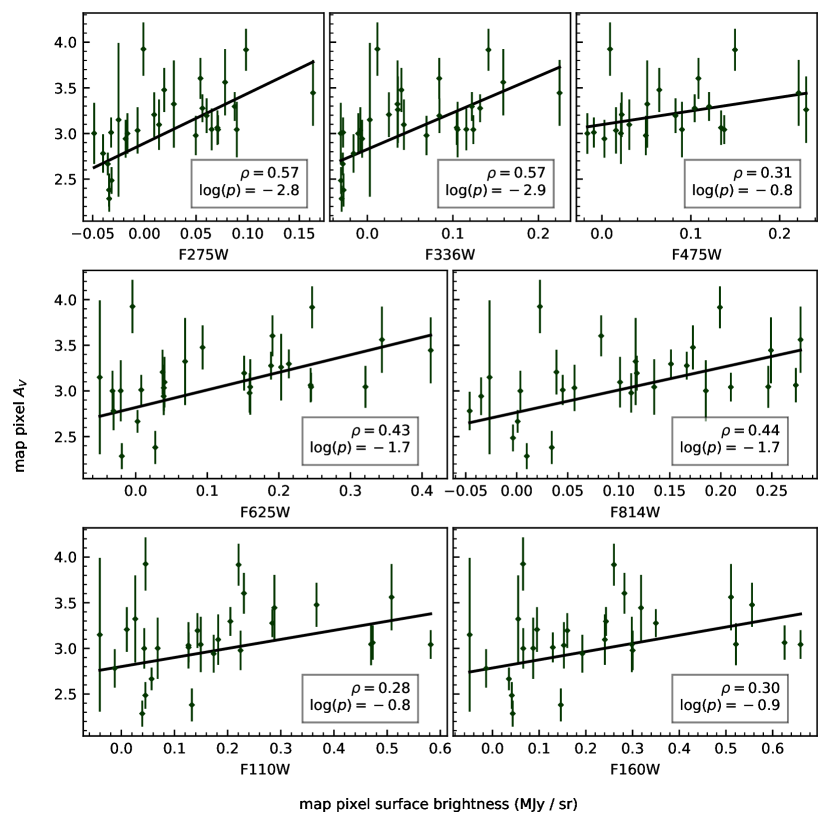
We investigate how our and maps compare to the dust emission measured using Spitzer and Herschel data. To look for a relation between and the surface brightness in the different bands, the IRAC, MIPS, PACS and SPIRE maps are first reprojected onto the same coordinate grid, using the reproject package for Python.333https://reproject.readthedocs.io/en/stable/ For each reprojected image, the pixels are matched with the ones from the map, and the reprojected fluxes are plotted against the map values, as shown in Figures 14 and 15. Upon applying the same analysis to the map, no significant correlation between any of the fluxes and was found.
| Band | ||
|---|---|---|
| () | () | |
| F275W | 0.183 | 0.025 |
| F336W | 0.250 | 0.035 |
| F475W | 0.669 | 0.350 |
| F625W | 0.520 | 0.094 |
| F814W | 0.408 | 0.069 |
| F110W | 1.007 | 0.239 |
| F160W | 1.115 | 0.242 |
| IRAC 3.6 | 2.472 | 0.332 |
| IRAC 4.5 | 1.216 | 0.164 |
| IRAC 5.8 | 11.770 | 1.563 |
| IRAC 8.0 | 33.961 | 4.387 |
| MIPS 24 | 26.741 | 3.496 |
| PACS 70 | 399.678 | 54.112 |
| PACS 160 | 345.684 | 45.670 |
| SPIRE 250 | 103.251 | 12.661 |
| SPIRE 350 | 38.976 | 4.734 |
| SPIRE 500 | 13.184 | 1.731 |
4.5 Model for the Average Dust SED
The surface brightness of dust with a single equilibrium temperature is given by
| (13) |
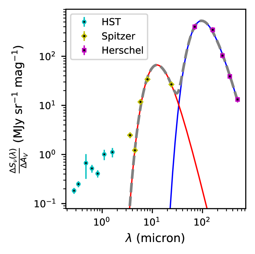
where is the grain absorption cross section per unit dust mass as a function of , is the dust surface mass density and is the Planck function. The subscript indicates that we are using quantities per unit frequency (e.g. MJy). Within this model with and as parameters, and are degenerate. But the quantity that we have measured, that is displayed in Figure 17 is actually the surface brightness per unit of :
| (14) |
So if a value for the ratio is known, it becomes possible to measure . In practice, we use a modified blackbody model of the form
| (15) |
as in 2014ApJ...797...85G. determines the effective value of at 160 micron. The second and third parameters are the and the effective temperature . These parameters are called effective because the observed surface brightness per is a mix of measurements along different sightlines, and each sightline is a mix of different dust populations. By using the well known relationship
| (16) |
we can write the model as
| (17) | ||||
| (18) |
where we drop the ‘eff’ subscript for conciseness. Therefore, by fitting this model to our measurements we can determine the average to V band opacity ratio. We treat the ratio as a single fit parameter.
We found that the sum of two modified blackbody models works well to fit the slopes calculated from the Herschel and Spitzer maps simultaneously. We use a least squares fitting approach using the standard options of Astropy’s modeling module. Three fit results are displayed in Table 4, and the corresponding curves are shown in 17.
| Fitting method | ||||||
|---|---|---|---|---|---|---|
| () | () | () | () | |||
| IndividualaaModel 1 is fit to the Herschel points, model 2 to the Spitzer points., free | ||||||
| Individual, fixed | 2.06 | 2.06 | ||||
| SimultaneousbbThe two models and sets of points are combined., fixed | 2.06 | 2.06 |
The first modified blackbody was fitted to only the PACS and SPIRE points, with a total of 0.61. The second model fit included the IRAC points and the MIPS 24 micron point, but not the IRAC 3.6 micron point. For this model, the -ratio and parameters are not well constrained, and in this case is 3.55. The estimated Pearson correlation coefficients between the three parameters are all over 90%, which is a known problem for this parametrization .
Fixing for both models gives stronger constraints on the other two parameters, especially on the temperatures. Lastly, we simultaneously fitted the sum of the two modified blackbodies with the same fixed value for , leading to the gray, dashed curve in Figure 17. For this two-component modified blackbody model, is 4.18 when fitting the 4 free parameters to our 9 data points, and the resulting parameters are shown on the third line of Table 4.
Using the same PACS 70 and 160 m images, and assuming a fixed , 2018A&A...619A.170A derive a color dust temperature of 30 K in IC 63. They also perform single-component modified blackbody fits with the same fixed at the tip of the nebula, and again obtain a dust temperature of K. This matches well with our value for . For the gas temperature, they report two values: K from H2 excitation diagrams, and 130 K from a PDR model.
As for the optical depth, 2018A&A...619A.170A find that . our value of , which is compatible with our value for . Multiplying the last two values for in 4 with 1.086 (eq. 16) gives us the result
| (19) | |||
| (20) |
In the above equations is the V-band cross section of the two components. We can compare the value of to theoretical dust models, using (the cross section at ) as an approximation for . With their standard grain size distributions, we find for the model of 2007ApJ...657..810D, and for the THEMIS model (2017A&A...602A..46J).
4.6 Per-pixel Modified Blackbody Fits
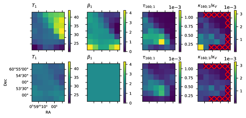
Instead of making a fit to the average SED obtained from the slopes, we also perform individual fits for each pixel of the maps, based on the same reprojected Spitzer and Herschel images. In this case, the scale parameter for the modified blackbodies is instead of , We are not fitting a differential measurement this time, and unlike the previous section we need to determine and subtract the background in each band. Since we have a measurement of the background of 2.51 mag, we use the slope and intercept of the lines in Figures 15 and 14 to calculate an appropriate level for the background in each band. By doing these per-pixel fits, we obtain maps of the same resolution for each parameter, .
Figure 18 shows a gradient in the temperature, perpendicular to the direction of the incoming radiation field. The typical uncertainty on is about 2 to 5 K. A feature of the same shape exists for the and parameters too, which shows an anticorrelation with the temperature. The relationship is well known and can be explained by variations in the dust properties . However, because of noise and temperature variations along the line of sight, least-squares fitting naturally leads to this type of correlation .
Comparing the map to the map in Figure 12, we find a similar structure. By dividing the values by the value in each pixel (minus the background of 2.51 mag), and using , we obtain maps of .
4.7 Comparison with other clouds
5 Conclusion
We have expanded the BEAST code to better support the fitting of background stars of nebulae and other nearby, transparent objects. We have performed individual SED fits of a combined stellar and extinction model to the numerous background stars of the IC 63 PDR, as observed by HST in seven broadband filters from the UV to the NIR.
From these fit results, we were able to generate maps of the extinction parameters and across the nebula. We find that varies between 0.5 and 1.4 mag when we assume a background of 2.5 mag. There is a decreasing trend in , from 3.7 at the tip of IC 63 to when moving further away from Cas. With a correction for background and/or foreground material, the latter value can go as low as .
It is the first time that this type of measurement has been made for a PDR. This approach was possible for IC 63 because of its low optical depth, making this PDR transparent for a sufficient number of detectable background sources. This same technique would therefore also be applicable to IC 59. Most other PDRs, such as the Horsehead nebula, have much higher optical depths and would not allow a sufficient amount of background stars to be measured.
By combining the map with FIR maps from Spitzer and Herschel, we were able to measure the shape of the average, -normalized surface brightness of the dust. A dual modified blackbody model fits the shape of this curve well, and provides two temperatures (30 and 227 K) and measurements of ( and ). By performing fits of the same model to individual pixels of the map, we derived a map of . The values of this map are of the same order of magnitude, but there are local variations which differ significantly (a factor 2 or 3) from the average.
Appendix A New BEAST feature: parallelization using subgrids
By introducing the stellar distance as an extra parameter, the dimensionality of the whole SED model grid is increased from 6D to 7D. Additionally the range of distances is potentially very large (see Table 2), and because the distance rescales the whole SED, a granularity on par with the grid is necessary. Since we chose to use (log spaced) distance bins, the amount of memory needed to work with the grid is also increased 40-fold. Originally we would split the catalog into many pieces, and then let every process work on a small part of the catalog. This approach is problematic because for every process launched, the whole grid has to be loaded into memory. Therefore, the total memory of the machine still imposes a limit on the number of fitting processes that can be run simultaneously.
To deal with these large grids, a memory-saving parallelization strategy was developed, which we call the subgridding approach. This approach entails that each process will work on only a small portion of the grid or subgrid. This works for the physics model setup, the noise model generation, as well as the fitting step. For each subgrid, a separate set of statistics and 1D posterior distributions is obtained. By properly taking into account the weight (integrated posterior) of each subgrid and combining these individual 1D posterior distributions, the statistics can be recalculated to reflect those of the whole grid.
To facilitate this parallelization scheme, a set of functions for splitting and/or merging the model grids and output statistics was developed, and an example workflow is given in the documentation.555https://beast.readthedocs.io/en/latest/subgrid_parallelism.html If the size of the RAM proves problematic for running the BEAST, then the number of subgrids can simply be increased. Arguably, this makes the BEAST scalable to much larger grid sizes.
Appendix B New BEAST feature: spatial variation of noise model
Since the extended emission varies for different locations in the nebula, the noise model should ideally depend on the position of the source that is being fit. To investigate the spatial dependence of the noise model, a set of tools was developed and added to the BEAST. The concept is that a number of regions on the sky that have similar intensities of background/foreground emission are determined (background regions). Within each of these background regions, a separate set of ASTs is performed, and an individual noise model is created. If the resulting noise models differ significantly, an individual fitting run can be done for each background region, using the corresponding noise model to fit only the sources that fall within that region.
B.1 Background map tool
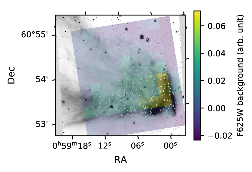
The first tool consists of a stand-alone script which can generate a map, with pixels of a user-specified size along the Right Ascension (RA) and Declination (Dec) axes. To measure the background for a single , it is first determined which of the sources of the input catalog fall into this bin, according to their positions. Then, a reference image is used (the F625W image in our case) to measure the background for each source. The sources themselves are masked out, and their background is determined using an annulus of a certain radius and thickness. Determining an ideal inner and outer radius for the annuli may require some trial and error by the user. The background for this is then set to be the median of these individual background measurements. For IC 63, the resulting background map is shown in the left panel of figure 19.
On a side note, this same tool can also be used to construct a map of point source densities in the exact same format. This is useful for catalogs that have a very high but variable density of stars, leading to different crowding effects depending on the position. The source density is derived directly from the positions listed in a given catalog. Since the rest of the code is agnostic of the quantity described by either map, a common approach can be used to model either effects of extended emission or those of crowding.
B.2 Selection of AST positions
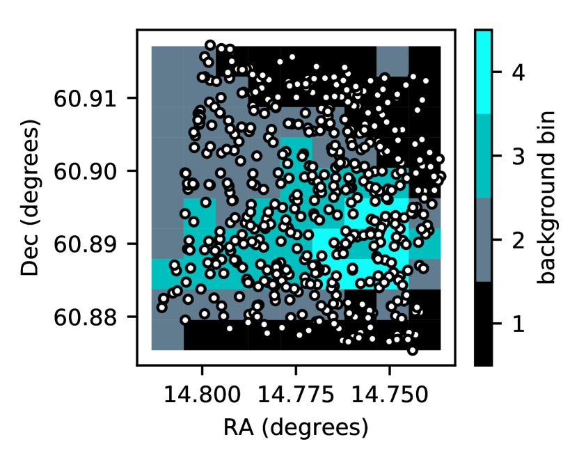
One of the applications that use this background map is the routine for selecting the positions of the ASTs. We want to make sure that the areas corresponding to different levels of background intensity are all sufficiently sampled. We achieve this by first choosing a set of bins (usually a small number, due to the available hard disk space and computing time), each of which represents a certain range in background intensity. Then, the of the map described above can be distributed among these bins, leading to groups of which constitute the desired background regions (Figure 19). A fixed set of SEDs is reused for each region, and each SED is assigned a random position within that region. This way, each background region has the same number of samples regardless of its total surface area.
B.3 Creating individual noise models
Once the selected ASTs have been run through our photometry routine, and a catalog of fake stars has been produced, both the observed and the fake catalog are split up according to the background regions (see again figure 19, right panel). By applying the same spatial split to both the observed catalog and the fake catalog, a series of catalog pairs is created. The BEAST can then use each pair consisting of one fake and one observed catalog to generate the individual noise models, and perform the individual fitting runs if the resulting noise models are found to be significantly different.
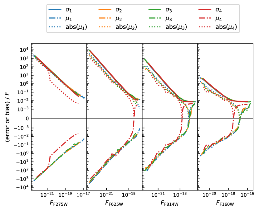
Using the regions shown in the right panel of Figure 19, we created four noise models (Figure 20). Despite the differences between the noise parameters for the background bins, we found that the predicted and are not significantly influenced by using these extra noise models. In each bin there are at most four stars which have an or that differs more than 10%. For some of the other parameters the differences can be larger, but the fit quality is not necessarily better. Therefore, the results presented in Section 3 and the rest of the analysis are based on fits using the single noise model that was shown in Figure 6. Note that this noise model still benefits from the background-based AST position picking, because it makes sure that the tip of the nebula is sufficiently sampled.
Appendix C The and maps in table format
We provide the values and standard deviation for and of the maps in Tables 5 and 6. The RA and Dec values in the table are the coordinates of the bottom left corner of each pixel, with the tables oriented in the same way as the color maps in Figure 12.
| Dec / RA (degrees) | 14.8021 | 14.7878 | 14.7736 | 14.7593 | 14.7450 | 14.7308 |
|---|---|---|---|---|---|---|
| 60.9206 | 3.54 ? | X | X | X | X | X |
| 60.9137 | 3.32 0.48 | 3.00 0.22 | 3.00 0.33 | 3.26 0.36 | 4.75 0.36 | X |
| 60.9067 | 3.92 0.29 | 3.10 0.28 | 3.03 0.25 | 3.01 0.16 | 5.12 0.45 | X |
| 60.8998 | 3.21 0.24 | 3.48 0.24 | 3.60 0.22 | 3.19 0.19 | 2.94 0.21 | 3.15 0.84 |
| 60.8928 | 3.04 0.30 | 3.28 0.15 | 3.06 0.19 | 3.92 0.23 | 3.04 0.23 | X |
| 60.8859 | 2.98 0.22 | 3.04 0.16 | 3.30 0.16 | 3.44 0.36 | 3.56 0.36 | X |
| 60.8790 | 2.67 0.12 | 2.78 0.21 | 2.38 0.18 | 2.29 0.14 | 2.49 0.15 | X |
| Dec / RA (degrees) | 14.8021 | 14.7878 | 14.7736 | 14.7593 | 14.7450 | 14.7308 |
|---|---|---|---|---|---|---|
| 60.9206 | 2.76 ? | X | X | X | X | X |
| 60.9137 | 3.44 0.11 | 3.73 0.14 | 3.48 0.10 | 3.47 0.15 | 3.75 0.36 | X |
| 60.9067 | 3.51 0.16 | 3.34 0.10 | 3.34 0.10 | 3.68 0.11 | 3.68 0.13 | X |
| 60.8998 | 3.43 0.14 | 3.52 0.11 | 3.45 0.14 | 3.55 0.07 | 3.59 0.11 | 3.60 0.25 |
| 60.8928 | 3.50 0.31 | 3.58 0.10 | 3.40 0.09 | 3.58 0.10 | 3.65 0.15 | X |
| 60.8859 | 3.31 0.09 | 3.53 0.16 | 3.72 0.14 | 3.63 0.15 | 3.66 0.26 | X |
| 60.8790 | 3.90 0.06 | 3.61 0.17 | 3.49 0.15 | 3.61 0.09 | 3.57 0.11 | X |