1 Motivation and Introduction
In many studies, it is possible to conduct and handle a large number of measurements, which makes high-dimensionality an increasingly important topic. In fact, high dimensional repeated measure designs or split-plot designs for multiple groups are the objectives of many analyses in science. This is the case in life science, where test persons were examined multiple times during a study, or in the industry where some parameters are measured on a nearly continuous basis.
Therein we consider measurements from subjects which are divided into independent and generally unbalanced groups where the i-th group contains observations.
Moreover, factor levels on the groups or repeated measures are possible. For independent -dimensional observation vectors null hypotheses regarding are investigated, where popular hypotheses are the existence of a group effect, a time effect as well as a interaction effect between time and group. For a classical repeated measure ANOVA design with , this was treated for example in Brunner et al., (2012). But in many cases, it is easier, cheaper or ethically more justifiable to increase the number of repetitions rather than increasing the sample size.
Therefore techniques are needed, which can handle the case of .
In the special case with just two groups but with a general distributional setting and without restriction on the dimension this was treated in Chen and Qin, (2010).
For more groups and a more general setting regarding hypotheses, Happ et al., (2016) uses a
classical ANOVA F test statistic, which has just an exact F-distribution for very special covariances matrices. So under some conditions on or the relation between the dimension and some power of traces containing the covariance matrix, they developed a decent approximation for the test statistic.
In Harrar and Kong, (2016) they handle several cases with an increasing number of groups under some requirements on the covariance matrices and the relation between sample sizes and the number of factor levels.
In contrast, Pauly et al., (2015) investigated the case with just one normal distributed group, but fewer assumptions on the covariance matric and no necessary relation between sample size and dimension.
Sattler and Pauly, (2018) expand these results especially for a larger number of groups, which is also allowed to approach infinity, together with the sample sizes and the dimension. Hereby, no restrictions on their respective convergence rate were made.
However, this does not treat the small large case which was, e.g., treated by Bathke, (2002) or Bathke and Lankowski, (2005) for fixed dimensions and balanced designs .
Therefore in addition to the large small case, we include the large small case, and further the combination of both, and develop a technique that can be used in each of these settings. To this end, we follow the same approach as Kong and Harrar, (2019) and assume homogenous covariance matrices with , again with no further assumptions on the structure of the covariance matrix . The homoscedastic setting allows some generalizations as well as a smaller number of other requirements on the underlying statistical model.
This paper is organized as follows. Section 2 introduces the statistical model, the investigated hypotheses and the notations used in the remaining paper. In Section 3 the test statistic is presented, as well as their asymptotic behavior and an alternative small sample approximation.
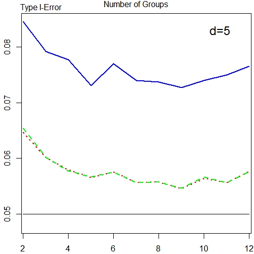
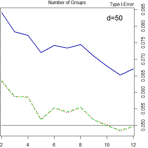
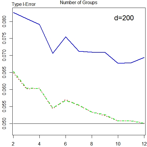
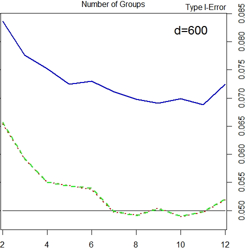
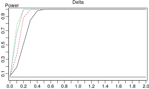
Section 4 contains simulations regarding the type-I-error rate and the power of the tests, introduced in the previous chapters.
The paper closes with a short conclusion. For brevity and readability, all proofs are shifted to the appendix.
2 Statistical Model and Hypotheses
We consider a homogenous split-plot design given by independent and unbalanced groups of -dimensional random vectors
|
|
|
(1) |
whereby each vector represents the measurement of one independent subject. It is assumed that mean vectors and one positive definite covariance
matrix exist.
As usual denotes the individual subjects or units in group , , so we have a total number of random vectors.
This framework allows a factorial structure regarding time, group or both, by splitting up the indices, accordingly, see Konietschke et al., (2015) for example.
Within this model linear hypotheses of repeated measures ANOVA,
formulated as
|
|
|
(2) |
are investigated.
Here, denots a proper hypothesis matrix , where and refer to whole-plot (group)
and/or subplot (time) effects, while denotes the Kronecker product.
For theoretical considerations it is often more convenient to reformulate through a corresponding projection matrix
, see e.g. Pauly et al., (2015).
Here denotes some generalized inverse of the matrix and can equivalently be written as
.
As discussed in Sattler and Pauly, (2018), has the form for projection matrices and . Now hypotheses of interest are for example given by
-
(a)
No group effect:
,
-
(b)
No time effect:
,
-
(c)
No interaction effect between time and group:
.
Here, is the d-dimensional matrix only containing 1s and is the centring matrix.
It is often useful to split the expectation vector into its components to simplify the interpretation.
With the common conditions , this can be done by expanding
|
|
|
Here, describes the -th group effect, the time effect at time point and
the -interaction effect between group and time. Thereby the above hypotheses can alternatively be formulated through
-
(a)
,
-
(b)
-
(c)
.
3 Test statistic and their asymptotic
In this work we consider the following 5 different asymptotic frameworks, which are:
|
|
|
(I) |
|
|
|
(II) |
|
|
|
(III) |
|
|
|
(IV) |
|
|
|
(V) |
This great diversity is exceptional and distinguishes from nearly all other approaches. Most of the existing procedures just consider special cases of one of these cases (for example Chen and Qin, (2010) (IV) with or Pauly et al., (2015) (IV) with ). Other allow for only one as Happ et al., (2016) for (IV) or Bathke, (2002) for (I).
In contrast, our framework allows the combination of any of these assumptions. However, alone is not included as this would not allow the construction of consistent trace estimators of covariances which are later needed for inference. Moreover, the case with fixed and has already been studied in detail in the literature and is, thus excluded here, see, e.g., Friedrich et al., (2017) or Bathke et al., (2018) and the references cited therein.
It is apparent that in contrast to Sattler and Pauly, (2018) and other papers, the common conditions as are missing. This is significant, because it allows an appreciably larger amount of settings, especially for . But it also clearly generalizes the model for the case of fixed , e.g. in unbalanced settings, where we only let some group sample sizes converge to .
To examine the validity of the nullhypothesis unattached from the asymptotic framework, we use
Here with denotes the vector of pooled group means.
Unfortunately for many covariance matrices , this random variable tends to converge to infinity, for or . To avoid this behaviour
the standardized quadratic form is given by
|
|
|
is used, which also enables us to evaluate all limit distributions in detail.
For normal distributed observations the expectation and variance of the quadratic form is known and it follows that
Observe, that for both values only the first factor resp. depends on the unknown covariance matrix, while all other quantities are known from the test setting.
Applying the representation theorem for quadratic forms in normaly distributed random vectors fromMathai and Provost, (1992) we can rewrite the standardized statistic as
|
|
|
(3) |
Here are the eigenvalues of in decreasing order, and is a sequence of independent
-distributed random variables. As a consequence, the asymptotic behaviour of the eigenvalues, determine the asymptotic limit distribution of . In fact, we obtain in generalization of Pauly et al., (2015) and Sattler and Pauly, (2018):
Theorem 3.1:
Let for .
Then has, under , and one of the
frameworks (I)-(V) asymptotically
-
a)
a distribution of the form , if and only if
|
|
|
for a decreasing sequence in with , while , .
-
b)
a distribution of the form , if
|
|
|
for a decreasing sequence in with and .
Putting the results into context. Chen and Qin, (2010) only considered case a) with . Sattler and Pauly, (2018) at least found asymptotic results in case b) but for case a) they need .
So this theorem is not only distinct from other results through the variety of asymptotic settings. It also enhances the continuum of limit distributions considerably through a mixture of normal distribution and finite sums of weighted standardized -distributed random variables. Furthermore, the if and only if relation shows the importance of the demands for the standardized eigenvalues and that it isn’t possible to relax them.
To use this test statistic it is necessary to construct proper estimators which are ratio consistent in all our settings. To this end, define
and
Below we prove that they are unbiased and ratio consistent estimators for and , respectivly, under both, the nullhypothesis and the alternative.
This allows us to define the estimated version of our test statistic by
|
|
|
The following Lemma justifies the usage of the estimated version instead of the exact one.
Theorem 3.2:
Under and one of the
frameworks (I)-(V) the statistic has the same asymptotic limit distributions as , if the respective conditions (a)-(b) from Theorem 3.1 are fulfilled.
Unfortunately the calculation of the standardized eigenvalues is in generally not simplified through homogeneity. Therefore it is nearly impossible to find an appropriate estimator which can be used in all our frameworks. Moreover simulations showed that large sample sizes dimension or number of groups are necessary for a good approximation, which make quantiles based on Theorem 3.1 a) difficult to apply. For similar reasons, in Pauly et al., (2015) and Sattler and Pauly, (2018) they used the quantils of a random variable of the kind
|
|
|
(4) |
in case of . The choice of for the degrees of freedom lead to a third moment approximation. In our homoscedastic model the usage of this random variable is based on the following theorem.
Theorem 3.3:
Under the conditions of Theorem 3.1 and one of the
frameworks (I)-(V) the random variable has, under , asymptotically
-
a)
a standard normal distribution if as ,
-
b)
a standardized distribution if as .
With the well known rules for the kronecker product and traces we can decompose this number by
|
|
|
The connection between and in the two extreme cases, i.e. if and only and if and only if , have been investigated in Pauly et al., (2015) for the case of but also translate to the present framework.
Here we have to estimate the first part, while the second one just depends on the asymptotic setting and therefore is known. This allows us to use the same estimated traces for different hypothesis which differ only in .
Moreover, for , we also have , without estimation, because . Otherwise, however, the behaviour of is unclear and we have to find consistent estimators for in all our different frameworks. This achieved by considering the class of estimators
|
|
|
which are based on suitable symmetrized U-statistics, while means that all indices are different.
Afterwards these estimators for each individual group are combined, to get an estimator which uses the observations of each group, given by
|
|
|
Together with the estimators from above, we can construct a consistent estimator for by .
Theorem 3.4:
In all our frameworks (I)-(V), it holds that
-
i)
is an unbiased estimator for ,
-
ii)
,
where denotes convergence in propabilty.
Through the usage of U-statistics with a kernel of order 6, for each estimator , summations have to be done. In contrast, estimators based on observations from all groups would require much higher numbers. For example in Sattler and Pauly, (2018) summations are necessary. Due to homogeneity, we don’t need this kind of estimator, but also requires summations, which is already really high, even for comparatively small samples sizes or numbers of groups. Thus, as in Sattler and Pauly, (2018), the usage of subsampling versions of our estimators is reasonable to make them applicable in practice. The underlying idea is instead of summing up all possible index combinations of one group we just do this for a randomly chosen subset of combinations.
To define the subsampling version, it is first necessary to introduce some definitions and notations.
A parameter is chosen and used to define as the number of subsampling repetitions done for the i-th group. It is clear that the choice of has a great influence on the calculation time and accuracy, so it should be chosen suitable for the situation.
Then, random subsamples of length from are drawn independently for each and , to define the subsampling version of by
|
|
|
Here
|
|
|
|
|
|
|
|
|
Combining them, allows to define the subsamling version of by
|
|
|
Theorem 3.5:
For , if (which includes frameworks (I)-(V)) it holds:
-
a)
is unbiased for .
-
b)
fullfilles
This way of defining the number of subsampling repetitions
, guarantees that the relation between the subsampled parts resembles the relation between the original . Although this can lead to great differences between the subsampling sizes for the different groups, it ensures that the influence of single groups is not too big.
These results allow to formulate a more useable version of through the following theorem.
Theorem 3.6:
The results of Theorem 3.3 remains valid if is replaced by or .
For the estimation of the unknown traces, it would also be possible to construct estimators that use observations from different groups. This is feasible and seems to be reasonable but in practice, we would again need subsampling versions of these estimators, which take care of the structure of the dataset. This is really complicated and therefore not usable in practice. So we avoid these difficulties by using estimators for the separate groups and combine them afterward.
Relaxing the assumption of homogeneous covariance matrices to with , which is essentially easier to fulfill, wouldn’t change the validity of the previous results. From a theoretical point of view it would be even sufficient to assume for , but this is nearly impossible to justify in practice.
6 Appendix
-
Proof of Theorem 3.1:
For this proof, it is helpful to present the theorem in a more detailed way.
Let for .
Then has, under , and one of the
frameworks I-V asymptotically
-
a)
a standard normal distribution if and only if
|
|
|
-
b)
a standardized distribution if and only if
|
|
|
-
c)
a distribution of the shape , if and only if
|
|
|
for a decreasing sequence in with with and with , .
-
d)
a distribution of the shape , if
|
|
|
for a decreasing sequence in with and .
The first two parts as well as the last one were proved in Sattler and Pauly, (2018).
For part c) from Cramers theorem it is well known that it needs an infinite number of summands to get a normal distribution as limit distribution. So it exists a infinite amount with
|
|
|
The proof of part a) shows, that for all , and because of the decreasing order there exists an with and .
Assume now that for otherwise consider the subsequence where this holds.
It remains to show that from
|
|
|
it follows as well as .
To this aim, we consider the Moment-generating functions so we know, for all
|
|
|
Thus, applying the continous mapping theorem we have for all
Now we consider the zero points of both sides which are a consequence of the polynomial parts and can be written by resp. . It can be directly inferred from this that both polyiomials has the same degree and therefore . Moreover both of them have the same zero points with the same multiplicity. So the coefficients are the same on both sides and because of the decreasing order it follows for .
Therefore the result follows.
∎
Given the fact that framework III is not really high-dimensional, and I just partwise, it would be possible to use other more classical estimators for the unknown traces. Nevertheless our focus was to develop preferably general estimators which can be used in a variety of settings.
Lemma 6.1:
With
|
|
|
we can define
|
|
|
which is an unbiased and ratio consistent estimator for , in all of our frameworks.
It is obvious that this is a unbiased estimator of . With well known rules and analogous to Sattler and Pauly, (2018) we calculate
|
|
|
Now we need a case analysis which is done for some of the following proofs. So the first one is in detail and the other proofs are shorter.
At first we consider the case where . Then
|
|
|
For the other case is bound and . In this situation it holds
|
|
|
So dividing by and then use the Tschebyscheff inequality leads to the results in both cases.
∎
For the estimated version of the standardized quadratic form, one more estimator is needed.
Lemma 6.2:
The estimator given by
|
|
|
is a unbiased and ratio-consistent estimator of in all our asymptotic frameworks.
-
Proof:
Again the unbiasedness is clear and we consider the variance.
We calculate
|
|
|
Similar as before for we get
|
|
|
and for bound and
|
|
|
Again the result follows by using Tschebyscheff’s inequality.
∎
With these theorems the usage of the estimated standardized quadratic form can be justified.
-
Proof of Theorem 3.2:
The result follows directly by theorem 3.2 from Sattler and Pauly, (2018).
∎
For the proof of Theorem 3.4 we need to show different properties that combined leads to the result.
We conduct this proof in several steps:
-
a)
-
b)
-
c)
in our frameworks I-V,
-
d)
in our frameworks I-V.
The results from Sattler and Pauly, (2018) directly yield to
|
|
|
and
|
|
|
which prooves a) and b). Together with Tschebychefs inequality this leads to an unbiased ratio consistent estimator for .
For part c) we calculate
|
|
|
and
|
|
|
|
|
|
Again this number is in for and in for . So in both cases the result follows with the Tschebyscheff-inequality.
At last the proof of part d) is done using the above results. A similar proof is part of Sattler and Pauly, (2018) but we repeat it for better understanding.
With the last lemma it follows for both cases that
were for the last step the trace inquality was used together with Slutzky’s theorem.
With the ratio-consistency of it follows and because of continous mapping . This leads to
∎
It is obvious that this estimator needs a sufficient big amount of groups with at least 6 observations. Similar for the other estimators, which were introduced earlier. From a theoretical point of view a scenario with is part of our model. In practice however, this setting is rarely examined. In this case, it would be possible to define some estimators which combine observations from different groups, which would be much more complicated than our estimators.
-
Proof of Theorem 3.5:
For this proof, some results of Sattler and Pauly, (2018) are used and adapted.
First the expactation value of the estimator, using the notation :
With Theorem A.9 Theorem A.10 and Theorem A.16 from Sattler and Pauly, (2018) for the variance we get
Again there the same to cases. If is bound and therefore is bound, it follows and hereby
while for which implies we calculate
first
and therefore
From this both values the results follows analogous to the proof of Theorem 3.4.∎
