Certified Adversarial Robustness for
Deep Reinforcement Learning

Abstract

Deep Neural Network-based systems are now the state-of-the-art in many robotics tasks, but their application in safety-critical domains remains dangerous without formal guarantees on network robustness. Small perturbations to sensor inputs (from noise or adversarial examples) are often enough to change network-based decisions, which was already shown to cause an autonomous vehicle to swerve into oncoming traffic. In light of these dangers, numerous algorithms have been developed as defensive mechanisms from these adversarial inputs, some of which provide formal robustness guarantees or certificates. This work leverages research on certified adversarial robustness to develop an online certified defense for deep reinforcement learning algorithms. The proposed defense computes guaranteed lower bounds on state-action values during execution to identify and choose the optimal action under a worst-case deviation in input space due to possible adversaries or noise. The approach is demonstrated on a Deep Q-Network policy and is shown to increase robustness to noise and adversaries in pedestrian collision avoidance scenarios and a classic control task.

Keywords: Adversarial Attacks, Reinforcement Learning, Collision Avoidance, Robustness Verification

1 Introduction

Deep reinforcement learning (RL) algorithms have achieved impressive success on robotic manipulation [1] and robot navigation in pedestrian crowds [2, 3]. Many of these systems utilize black-box predictions from deep neural networks (DNNs) to achieve state-of-the-art performance in prediction and planning tasks. However, the lack of formal robustness guarantees for DNNs currently limits their application in safety-critical domains, such as collision avoidance. In particular, even subtle perturbations to the input, known as adversarial examples, can lead to incorrect (but highly-confident) predictions from DNNs [4, 5, 6]. Furthermore, several recent works have demonstrated the danger of adversarial examples in real-world situations [7, 8], including causing an autonomous vehicle to swerve into oncoming traffic [9]. The work in this paper addresses the lack of robustness against adversarial examples and sensor noise by proposing an online certified defense to add onto existing deep RL algorithms during execution.

Existing methods to defend against adversaries, such as adversarial training [10, 11, 12], defensive distillation [13], or model ensembles [14] do not come with theoretical guarantees for reliably improving the robustness and are often ineffective on the advent of more advanced adversarial attacks [15, 16, 17, 18]. Verification methods do provide formal guarantees on the robustness of a given network, but finding the guarantees is an NP-complete problem and computationally intractable to solve in real-time for applications like robot manipulation or navigation [19, 20, 21, 22, 23]. Robustness certification methods relax the problem to make it tractable. Given an adversarial distortion of a nominal input, instead of finding exact bounds on the worst-case output deviation, these methods efficiently find certified lower bounds [24, 25, 26, 27, 28]. In particular, the work by [26] runs in real-time for small networks ($33$ to $14,000$ times faster than verification methods), its bound has been shown to be within $10\%$ error of the true bound, and it is compatible with many activation functions and neural network architectures [29, 30]. These methods were applied on computer vision tasks.

Figure 1: Intuition. An adversary distorts the true position, $s_{0}$, of a dynamic obstacle (blue) into an adversarial observation, $s_{adv}$. The agent (orange) only sees the adversarial input, so nominal RL policies would take $a^{*}_{nom}$ to reach the goal quickly, but would then collide with the true obstacle, $s_{0}$. The proposed defensive strategy considers that $s_{0}$ could be anywhere inside the $\epsilon$-ball around $s_{adv}$, and selects the action, ${a^{*}_{adv}}$, with the best, worst-case outcome as calculated by a guaranteed lower bound on the value network output, which cautiously avoids the obstacle while reaching the goal. Note this is different from simply inflating the obstacle radius, since the action values contain information about environment dynamics, e.g., blue agent’s cooperativeness.

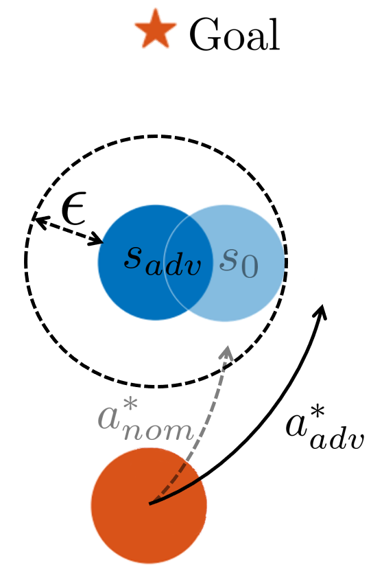
This work extends the tools for robustness certification against adversaries to deep RL tasks. As a motivating example, consider the collision avoidance setting in Fig. 1, in which an adversary perturbs an agent’s (orange) observation of an obstacle (blue). An agent following a nominal/standard deep RL policy would observe $s_{adv}$ and select an action, $a^{*}_{nom}$, that collides with the obstacle’s true position, $s_{0}$, thinking that space is unoccupied. Our proposed approach assumes a worst-case deviation of the observed input, $s_{adv}$, bounded by $\epsilon$, and takes the optimal action, $a^{*}_{adv}$, under that perturbation, to safely avoid the true obstacle. Nominal robustness certification algorithms assume $\epsilon$ is a scalar, which makes sense for image inputs (all pixels have same scale, e.g., $0{-}255$ intensity). A key challenge in direct application to RL tasks is that the observation vector (network input) could have elements with substantially different scales (e.g., position, angle, joint torques) and associated measurement uncertainties, motivating our extension with $\epsilon$ as a vector.

This work contributes (i) the first formulation of robustness certification deep RL problems, (ii) an extension of existing robustness certification algorithms to variable scale inputs, (iii) an optimal action selection rule under worst-case state perturbations, and (iv) demonstrations of increased robustness to adversaries and sensor noise on cartpole and a pedestrian collision avoidance simulation.

2 Related work

2.1 Varieties of adversaries in RL

RL literature proposes many approaches to achieve adversarial robustness. Domain Randomization, also called perturbed simulation, adversarially chooses parameters that guide the physics of a simulation, such as mass, center of gravity, or friction during training [31, 32]. Other work investigates the addition of adversarially acting agents [33, 34] during training. The resulting policies are more robust to a distribution shift in the underlying physics from simulation to real-world, e.g., dynamics/kinematics. This work, in comparison, addresses adversarial threats in the observation space, not the underlying physics [35]. For example, adversarial threats could be created by small perturbations in a camera image, lidar pointcloud, or estimated positions/velocities of pedestrians.

2.2 Defenses to adversarial examples

Much of the existing work on robustness against adversarial attacks detects or defends against adversarial examples. Adversarial training or retraining augments the training dataset with adversaries [10, 11, 12] to increase robustness during testing (empirically). Other works increase robustness through distilling networks [13], comparing the output of model ensembles [14], or detect adversarial examples through comparing the input with a binary filtered transformation of the input [36]. Although these approaches show impressive empirical success, they do not come with theoretical guarantees for reliably improving the robustness against a variety of adversarial attacks and are often ineffective against more sophisticated adversarial attacks [15, 16, 17, 18].

2.3 Formal robustness verification and certification

Verification methods provide these desired theoretical guarantees. The methods find theoretically proven bounds on the maximum output deviation, given a bounded input perturbation [19, 20, 21]. These methods rely on satisfiability modulo theory (SMT) [22, 19, 23], LP, or mixed-integer linear programming (MILP) solvers [20, 21], or zonotopes [37], to propagate constraints on the input space to the output space. The difficulty in this propagation arises through ReLU or other activation functions, which can be nonlinear in between the upper and lower bound of the propagated input perturbation. In fact, the problem of finding the exact verification bounds is NP-complete [19, 26] and thus currently infeasible to be run online on a robot. A relaxed version of the verification problem provides certified bounds on the output deviation, given an input perturbation [24, 25, 26, 27, 28]. Fast-Lin [26], offers the certification of CIFAR networks in tens of seconds, provable guarantees, and the extendability to all possible activation functions [29]. This work extends Fast-Lin from computer vision tasks to be applicable in Deep RL domains.

2.4 Safe and risk-sensitive reinforcement learning

Like this work, several Safe RL algorithms surveyed in [38] also optimize a worst-case criterion. Those algorithms, also called risk-sensitive RL, optimize for the reward under worst-case assumptions of environment stochasticity, rather than optimizing for the expected reward [39, 40, 41]. The resulting policies are more risk-sensitive, i.e., robust to stochastic deviations in the input space, e.g., sensor noise, but could still fail on algorithmically-crafted adversarial examples. To be fully robust against adversaries, this work assumes a worst-case deviation of the input space inside some bounds and takes the action with maximum expected reward. A concurrent line of work trains an agent to not change actions in the presence of adversaries, but does not guarantee that the agent takes the best action under a worst case perturbation [42].Other work in Safe RL focuses on parameter/model uncertainty, e.g., uncertainty in the model for novel observations (far from training data) in [43, 44]. Several robotics works avoid the sim-to-real transfer by learning policies online in the real world. However, learning in the real world is slow (requires many samples) and does not come with full safety guarantees [45, 46].

3 Background

3.1 Robustness certification

In RL problems, the state-action value $Q=\mathbb{E}[\sum_{t=0}^{T}{\gamma^{t}r_{t}}]$ expresses the expected future reward, $r_{t}$, discounted by $\gamma$, from taking an action in a given state/observation. This work aims to find the action that maximizes state-action value under a worst-case perturbation of the observation by sensor noise or an adversary. This section explains how to obtain the certified lower bound on the DNN-predicted $Q$, given a bounded perturbation in the input space from the true state. The derivation is based on [26], re-formulated for RL. We define the certified lower bound of the state-action value, $Q_{L}$, for each discrete action, $a_{j}$, as

$$Q_{L}(s_{adv},a_{j}):=\min_{s\in B_{p}(s_{adv},\epsilon)}Q_{l}(s,a_{j}),$$ (1)

for all possible states, $s$, inside the $\epsilon$-Ball around the observed input, $s_{adv}{\in}\mathbb{R}^{n}$, where $B_{p}(s_{adv},\epsilon):=\{s:\;\lvert\lvert s-s_{adv}\rvert\rvert_{p}\leq\epsilon\}$. $Q_{l}$ is the certified lower bound for a given state: $Q_{l}(s,a_{j})\leq Q(s,a_{j})\forall s\in B_{p}(s_{adv},\epsilon),\forall a_{j}{\in}\mathds{A}$, and calculated in Eq. 3. The $L_{p}$-norm bounds the input deviation that the adversary was allowed to apply, and is defined as $\lvert\lvert x\rvert\rvert_{p}=(\lvert x_{1}\lvert^{p}+...+\lvert x_{n}\lvert^{p})^{1/p}$ for $x{\in}\mathbb{R}^{n}$, $p{\geq}1$.

The certification essentially passes the interval bounds $[l^{(0)},u^{(0)}]=[s_{adv}-\epsilon,s_{adv}+\epsilon]$ from the DNN’s input layer to the output layer, where $l^{(k)}$ and $u^{(k)}$ denotes the lower and upper bound of the preReLU-activation, $z^{(k)}$, in the $k$-th layer of an $m$-layer DNN. The difficulty while passing these bounds from layer to layer arises through the nonlinear activation functions, such as ReLU, PReLU, tanh, sigmoid. Note that although this work considers ReLU activations, it can easily be extended to general activation functions via the certification process as seen in [29]. When passing interval bounds through a ReLU activation, the upper and lower preReLU bound can either both positive $(l^{(k)},u^{(k)}>0)$, negative $(l^{(k)},u^{(k)}<0)$, or positive and negative $(l^{(k)}<0,u^{(k)}>0)$, in which the ReLU status is called active, inactive or undecided, respectively. In the active and inactive case, bounds are passed to the next layer as normal. In the undecided case, the output of the ReLU is bounded through linear upper and lower bounds:

$$\sigma_{[l^{(k)},u^{(k)}]}(z^{(k)})=\begin{cases}[z^{(k)},z^{(k)}]&\text{if $l^{(k)},u^{(k)}>0$, ``active''}\\ [0,0]&\text{if $l^{(k)},u^{(k)}<0$, ``inactive''}\\ [\frac{u^{(k)}}{u^{(k)}-l^{(k)}}z^{(k)},\frac{u^{(k)}}{u^{(k)}-l^{(k)}}(z^{(k)}-l^{(k)})]&\text{if $l^{(k)}{<}0,u^{(k)}{>}0$, ``undecided''.}\end{cases}$$ (2)

The identity matrix $D$ is introduced as the ReLU status matrix, $H$ as the lower/upper bounding factor, $W$ as the weight matrix, $b$ as the bias in layer $(k)$ with $r,j$ as indices, and the preReLU-activation, $z^{(k)}$, is replaced with $W_{r,:}^{(k)}s+b_{r}^{(k)}$. The ReLU bounding is then rewritten as

$$D_{r,r}^{(k)}(W_{r,j}^{(k)}s_{j}+b_{r}^{(k)})\leq\sigma(W_{r,j}^{(k)}s_{j}+b_{r}^{(k)})\leq D_{r,r}^{(k)}(W_{r,j}^{(k)}s_{j}+b_{r}^{(k)}-H_{r,j}^{(k)}),$$

$$\text{where }D_{r,r}^{(k)}=\begin{cases}\frac{u_{r}^{(k)}}{u_{r}^{(k)}-l_{r}^{(k)}}&\text{if $l_{r}^{(k)}{<}0,u_{r}^{(k)}{>}0$;}\\ 1&\text{if $l_{r}^{(k)},u_{r}^{(k)}{>}0$;}\\ 0&\text{if $l_{r}^{(k)},u_{r}^{(k)}{<}0$,}\end{cases}\text{and }H_{r,j}^{(k)}=\begin{cases}l_{r}^{(k)}&\text{if $l_{r}^{(k)}{<}0,u_{r}^{(k)}{>}0,A_{j,r}^{(k)}{<}0$;}\\ 0&\text{otherwise.}\end{cases}$$

Similar to the closed-form forward pass in a DNN, one can formulate the closed form solution for the guaranteed lower bound of the state-action value for a single state $s$:

$$Q_{l}(s,a_{j})=A_{j,:}^{(0)}s+b_{j}^{(m)}+\sum_{k=1}^{m-1}{A_{j,:}^{(k)}(b^{(k)}-H_{:,j}^{(k)})},$$ (3)

where the matrix $A$ contains the network weights and ReLU activation, recursively for all layers: $A^{(k-1)}=A^{(k)}W^{(k)}D^{(k-1)}$, with identity in the final layer: $A^{(m)}=\mathds{1}$.

3.2 Pedestrian simulation

Among the many RL tasks, a particularly challenging safety-critical task is collision avoidance for a robotic vehicle among pedestrians. Because learning a policy in the real world is dangerous and time consuming, this work uses a kinematic simulation environment for learning pedestrian avoidance policies. The decision process of an RL agent in the environment can be described as Partially Observable Markov Decision Process (POMDP) with the tuple $<S,\mathds{A},T,R,\Omega,O,\gamma>$. The environment state $S$ is fully described by the behavior policy, position, velocity, radius, and goal position of each agent. In this example, the RL policy controls one of two agents with 11 discrete action heading actions $A=[a_{\min},a_{\max}]=[-\pi/6,+\pi/6]$ and constant velocity $v=1m/s$. The environment executes the selected action under unicycle kinematics, and controls the other agent from a diverse set of fixed policies (static, non-cooperative, ORCA [47], GA3C-CADRL [3]). The sparse reward is $1$ for reaching the goal, $-0.25$ for colliding and the partial observation is the x-y position, x-y velocity, and radius of each agent, and the RL agent’s goal, as in [3].

4 Approach

This work develops an add-on certified defense for existing Deep RL algorithms to ensure robustness against sensor noise or adversarial examples during test time.

4.1 System architecture

Figure 2: System Architecture. During online execution, an agent observes a state, $s_{adv}$, corrupted by sensor noise or an adversarial attack. A Deep RL algorithm, e.g., Deep Q-Network (DQN) [48], predicts the state-action values, $Q$. A node for certified defense accesses the predicting network, adds a robustness threshold $\pm\epsilon$ in the input space and computes a lower bound of the state-action values of each discrete action: $Q_{L}$. The agent takes the action, $a^{*}$, that maximizes the lower bound, i.e. is the most robust to the deviation in the input space.

Figure 2 depicts the system architecture of a standard model-free RL framework with the added-on certification. In an offline training phase, an agent uses a deep RL algorithm, here DQN [48], to train a DNN that maps non-corrupted state observations, $s$, to state-action values, $Q(s,a)$. Action selection during training uses the nominal cost function, $a^{*}_{nom}=\operatorname*{\arg\!\max}_{a}Q(s,a)$. We assume the training process causes the network to converge to the optimal value function, $Q^{*}(s,a)$ and focus on the challenge of handling perturbed observations during execution.

During online execution, the agent only receives corrupted state observations from the environment, and passes those through the DNN. The certification node uses the DNN architecture and weights, $W$, to compute lower bounds on $Q$ under a bounded perturbation of the input $s\pm\epsilon$, which are used for robust action selection during execution (described below).

4.2 Optimal cost function under worst-case perturbation

We consider robustness to an adversary who picks the worst-possible state observation, $s_{adv}$, within a small perturbation, $\epsilon$, of the true state, $s_{0}$. The adversary assumes the RL agent follows a nominal policy (as in e.g., DQN) of selecting the action with highest Q-value at the current observation. A worst possible state observation, $s_{adv}$, is therefore any one which causes the RL agent to take the action with lowest Q-value in the true state $s_{0}$,

$$s_{adv}\in\{s:\;s\in B_{p}(s_{0},\epsilon)\,\text{and}\,\operatorname*{\arg\!\max}_{a}Q(s,a)=\operatorname*{\arg\!\min}_{a}Q(s_{0},a)\}$$ (4)

After the adversary picks the state observation, the agent selects an action. Instead of trusting the observation (and thus choosing the worst action for the true state), the agent leverages the fact that the true state $s_{0}$ could be anywhere inside an $\epsilon$-Ball around $s_{adv}$: $s_{0}\in B_{p}(s_{adv},\epsilon)$. The agent evaluates each action by calculating the worst-case Q-value under all the possible true states. The optimal action, $a^{*}$, is defined here as one with the highest Q-value under the worst-case perturbation,

$$a^{*}=\operatorname*{\arg\!\max}_{a_{j}}\min_{s\in B_{p}(s_{adv},\epsilon)}Q_{l}(s,a_{j})=\operatorname*{\arg\!\max}_{a_{j}}Q_{L}(s_{adv},a_{j}),$$ (5)

using the outcome of the certification process, $Q_{L}$, as defined in Eq. 1.

4.3 Adapting robustness certification to deep RL

To solve Eq. 5 when $Q(s,a)$ is represented by a DNN, we adapt the formulation from [26]. Most works in adversarial examples, including [26], focus on defending adversaries on image inputs, in which all channels have the same scale, e.g. black/white images with intensities in $[0,255]$. More generally, however, input channels could be on different scales, e.g. joint torques, velocities, positions. Although not often mentioned, these sensor readings can also be prone to adversarial attacks, if transmitted over an insecure messaging framework, e.g. ROS, or accidentally producing adversaries through sensor failure or noise. Hence, this work extends [26] to certify robustness of variable scale inputs and enables the usage to the broader robotics and machine learning community.

To do so, we compute the lower bound $Q_{L}(s_{adv},a_{j})$ for all states inside the $\epsilon$-Ball $B_{p}(s_{adv},\epsilon)$ around $s_{adv}$ similar to [26], but with vector $\epsilon$ (instead of scalar $\epsilon$):

$$Q_{L}(s_{adv},a_{j}) =\min_{s\in B_{p}(s_{adv},\epsilon)}\left(A_{j,:}^{(0)}s+b_{j}^{(m)}+\sum_{k=1}^{m-1}{A_{j,:}^{(k)}(b^{(k)}-H_{:,j}^{(k)})}\right)$$ (6)

$$=\left(\min_{s\in B_{p}(s_{adv},\epsilon)}A_{j,:}^{(0)}s\right)+b_{j}^{(m)}+\sum_{k=1}^{m-1}{A_{j,:}^{(k)}(b^{(k)}-H_{:,j}^{(k)})}$$ (7)

$$=\left(\min_{y\in B_{p}(0,1)}A_{j,:}^{(0)}(y\circ\epsilon)\right)+A_{j,:}^{(0)}s_{adv}+b_{j}^{(m)}+\sum_{k=1}^{m-1}{A_{j,:}^{(k)}(b^{(k)}-H_{:,j}^{(k)})}$$ (8)

$$=\left(\min_{y\in B_{p}(0,1)}(\epsilon\circ A_{j,:}^{(0)})y\right)+A_{j,:}^{(0)}s_{adv}+b_{j}^{(m)}+\sum_{k=1}^{m-1}{A_{j,:}^{(k)}(b^{(k)}-H_{:,j}^{(k)})}$$ (9)

$$=-\lvert\lvert\epsilon\circ A_{j,:}^{(0)}\rvert\rvert_{q}+A_{j,:}^{(0)}s_{adv}+b_{j}^{(m)}+\sum_{k=1}^{m-1}{A_{j,:}^{(k)}(b^{(k)}-H_{:,j}^{(k)})},$$ (10)

with $\circ$ denoting element-wise multiplication. From Eq. 7 to Eq. 8, substitute ${s:=y\circ\epsilon+s_{adv}}$, to shift and re-scale the observation to within the unit ball around zero, $y\in B_{p}(0,1)$. The maximization in Eq. 9 reduces to a q-norm in Eq. 10 by the definition of the dual norm $\lvert\lvert z\rvert\rvert_{*}=\{\text{sup}z^{T}y:\lvert\lvert y\rvert\rvert\leq 1\}$ and the fact the $l_{q}$ norm is dual of $l_{p}$ norm for $p,q\in[1,\infty)$ (with $1/p+1/q=1$). The closed form in Eq. 10 is inserted into Eq. 5 to return the best action.

5 Experimental Results

The robustness against adversaries and noise during execution is evaluated in simulations for collision avoidance among pedestrians and the cartpole domain. In both domains, increasing magnitudes of noise or adversarial attacks are added onto the observations, which reduces the reward of an agent following a nominal non-robust DQN policy. The added-on defense with robustness parameter, $\epsilon$, increases the robustness of the policy to the introduced perturbations and increases the performance.

5.1 Adversarially robust collision avoidance

A nominal DQN policy was trained in the environment described in Section 3.2. To evaluate the learned policy’s robustness to deviations of the input in an $\epsilon$-ball, $B_{p}(s_{0},\epsilon)$, around the true state, $s_{0}$, the observations of the environment agent’s position are deviated by an added uniform noise ${\sim}\mathbb{U}([-\sigma,\sigma])$, or adversarial attack during testing. The adversarial attack is a fast gradient sign method with target (FGST) [7] and approximates the adversary from Eq. 4. FGST crafts the state $\hat{s}_{adv}$ on the $\epsilon$-Ball’s perimeter that maximizes the Q-value for the nominally worst action $\operatorname*{\arg\!\min}_{a}Q(s_{0},a)$. Specifically, $\hat{s}_{adv}$ is picked along the direction of lowest softmax-cross-entropy loss, $\mathbb{L}$, in between a one-hot encoding $y_{adv}$ of the worst action and the nominal Q-values, $y_{nom}$:

$$\hat{s}_{adv}=s_{0}-\epsilon_{adv}\;\text{sign}(\nabla_{s}\mathbb{L}(y_{adv},y_{nom}))$$

$$y_{adv}=[\mathds{1}\{a_{i}={\mathop{\mathrm{argmin}}\nolimits}_{a}Q(s_{0},a)\}]\in\mathbb{R}^{\lvert\mathds{A}\rvert}$$

$$y_{nom}=[Q(s_{0},a_{i})]\in\mathbb{R}^{\lvert\mathds{A}\rvert}$$

As expected, the nominal DQN policy, $\epsilon{=}0$, is not robust to the perturbation of inputs: Increasing the magnitude of adversarial, or noisy perturbation, $\epsilon_{adv},\sigma$ drastically 1) increases the average number of collisions (as seen in  Figs. 3 and 3, respectively, at $\epsilon{=}0$) and 2) decreases the average reward (as seen in  Figs. 3 and 3). The number of collisions and the reward are reported per run and have been averaged over $5$x$100$ episodes in the stochastic environment. Every set of $500$ episodes constitutes one data point, $*$, and has been initialized with the same $5$ random seeds.

(a)

(b)

(c)

(d)

Figure 3: Robustness against adversarial attacks and noise. Figures 3 and 3 shows that an increasing robustness parameter, $\epsilon$, decreases the number of collisions in the existence of adversarial attacks, or noise with increasing magnitude $\epsilon_{adv},\sigma$. Figures 3 and 3 show that an increasing robustness parameter $\epsilon$ increases the reward for several magnitudes of adversarial attacks or noise (e.g., $\epsilon_{adv}{=}0.17m,\sigma{=}0.28m$) while $\epsilon<{\sim 0.2}$.

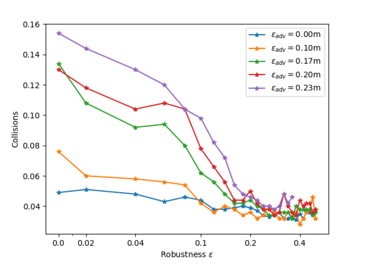
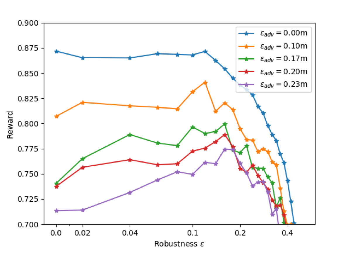
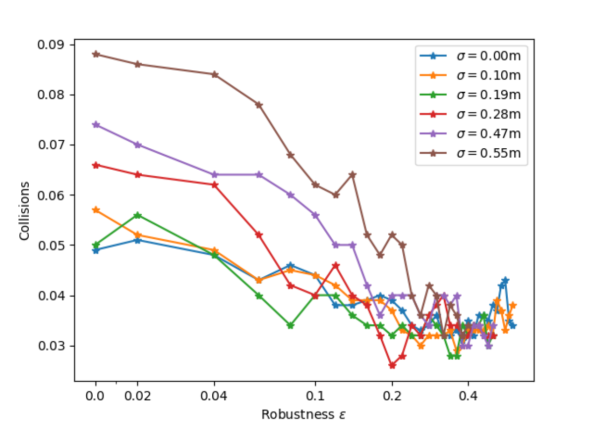
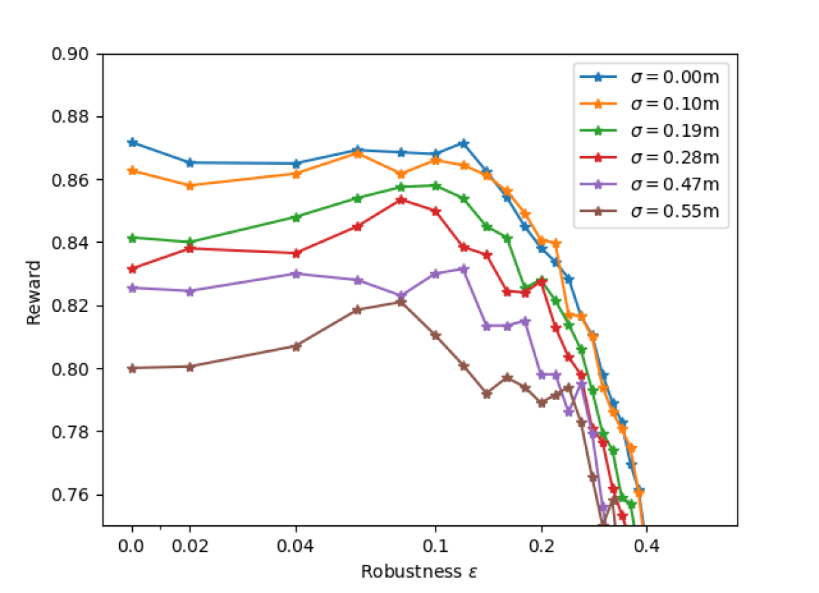
Next, we demonstrate the effectiveness of the proposed add-on defense, called Certified Adversarially-Robust Reinforcement Learning (CARRL). The number of collisions decreases with an increasing robustness parameter $\epsilon$ under varying magnitudes of noise, or adversarial attack, as seen in Figs. 3 and 3. As a result, the reward increases with an increasing robustness parameter $\epsilon{<}{\sim}0.1$ under varying magnitudes of perturbations, as seen in Figs. 3 and 3. As expected, the importance of the proposed defense is highest under strong perturbations, as seen in the strong slopes of the curves $\epsilon_{adv}{=}0.23m$ and $\sigma{=}0.55m$. Interestingly, the CARRL policy only marginally reduces the reward under no perturbations, $\sigma{=}0,\epsilon_{adv}{=}0$.

Since the CARRL agent selects actions more conservatively than a nominal DQN agent, it is able successfully reach its goal instead of colliding like the nominal DQN agent does under noisy or adversarial perturbations. Interestingly, the reward drops significantly for $\epsilon{>}{\sim}0.1$, because the agent “runs away” from the obstacle and never reaches the goal, also seen in Fig. 6. This is likely due to the relatively small exploration of the full state space while training the Q-network. $\epsilon{>}0.1$ yields an $\epsilon$-ball around $s_{adv}$ that is too large and contains states that are far from the training data, causing our learned Q-function to be inaccurate, which breaks CARRL’s assumption of a perfectly learned Q-function for $\epsilon>{\sim}0.1$. However, even with a perfectly learned Q-function, the agent could run away or stop, when all possible actions could lead to a collision, similar to the freezing robot problem [49].

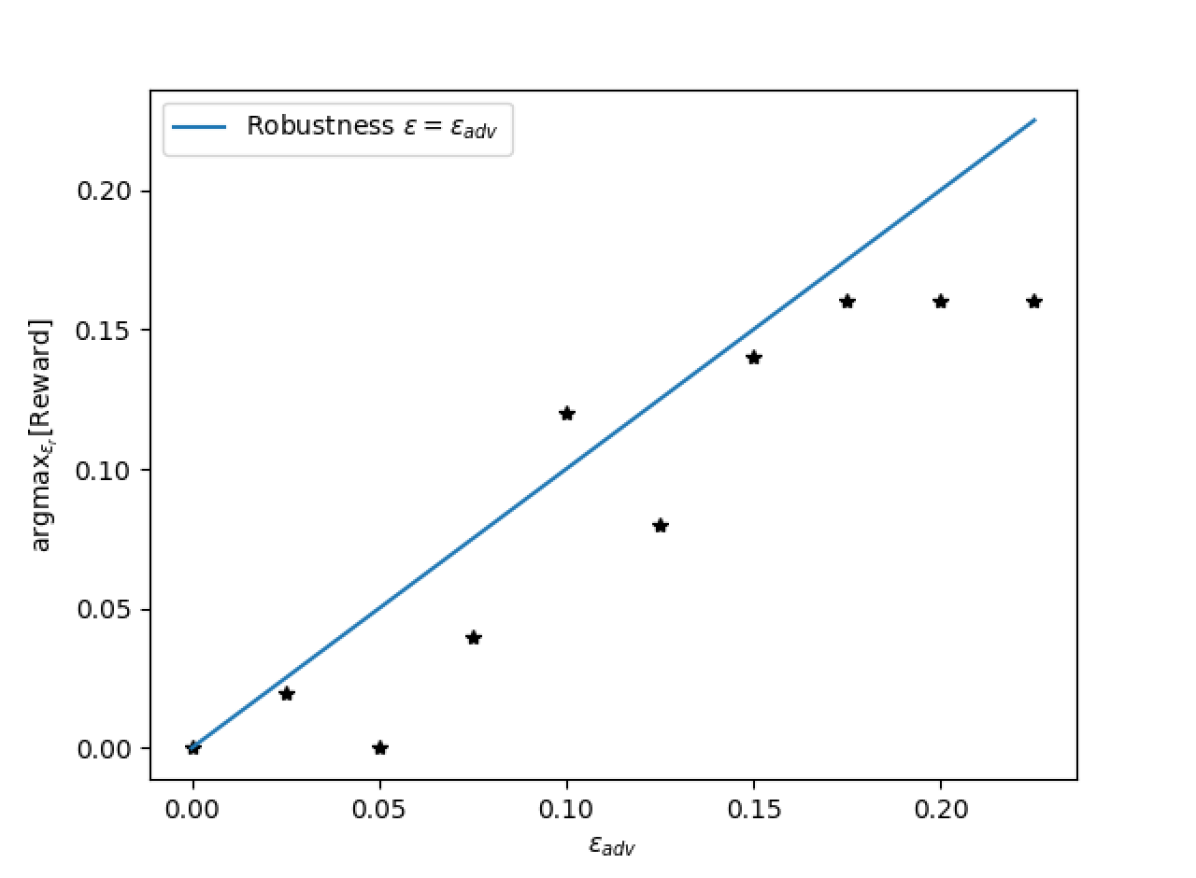
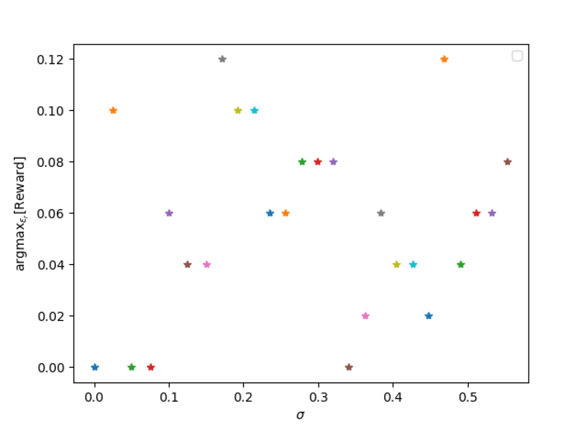
Figure 4 illustrates further intuition on choosing $\epsilon$. Figure 4 demonstrates a linear correlation in between the attack magnitude $\epsilon_{adv}$ and the best defending $\epsilon$ from Fig. 3, i.e., the $\epsilon$ that maximizes the reward under the given attack magnitude $\epsilon_{best}=\operatorname*{\arg\!\max}_{\epsilon\in[\epsilon_{min},\epsilon_{max}]}R(\epsilon,\epsilon_{adv})$. A correlation cannot be observed under sensor noise, as seen in Fig. 4, because an adversary chooses an input state on the perimeter of the $\epsilon$-ball, whereas uniform noise samples from inside the $\epsilon$-ball. The $p{=}\infty$-norm has been chosen for robustness against uniform noise and the FGST attack, as position observations could be anywhere within a 2-D box around the true state. The modularity in $\epsilon$ allows CARRL to capture uncertainties of varying scales in the input space, e.g., $\epsilon$ is here non-zero for position and zero for other inputs, but could additionally be set non-zero for velocities. $\epsilon$ can further be adapted on-line to account for, e.g., time-varying sensor noise.

(a)

(b)

Figure 4: Correlation between perturbation magnitude and $\epsilon$ robustness. Figure 4 shows that the magnitude of the adversarial attack, $\epsilon_{adv}$, is linearly correlated with the best robustness, $\epsilon$ (i.e., one that maximizes the reward under a given attack magnitude). Figure 4 shows that this correlation does not exist when defending against noise. A possible explanation is that an adversary chooses an input state on the perimeter of the $\epsilon$-ball, whereas uniform noise samples from inside the $\epsilon$-ball.

The CARRL policy is able run at real-time; querying the policy took ${\sim}20ms$. One forward pass with certified bounds took ${\sim}2ms$, which compares to a forward pass of our nominal DQN of ${\sim}1ms$. In our implementation, we inefficiently query the network once for each of the $11$ actions. The runtime could be reduced by parallelizing the action queries and should remain low for larger networks, as  [26] shows that the runtime scales linearly with the network size.

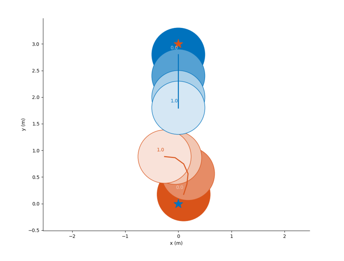
Visualization of the CARRL policy in particular scenarios offers additional intuition on the resulting policy. In Fig. 5, an agent (orange) with radius $.5m$ (circle) observes a dynamic obstacle (blue) with added uniform noise $\sigma{=}.4m$ (not illustrated) on the position observation. The nominal DQN agent, in Fig. 5 is not robust to the noise and collides with the obstacle. The CARRL policy, in Fig. 5, however, is robust to the small perturbation in the input space and successfully avoids the dynamic obstacle. The resulting trajectories for several $\epsilon$ values are shown in Fig. 6, for the same uniform noise addition. With increasing $\epsilon$ (toward right), the CARRL agent accounts for increasingly large worst-case position perturbations. Accordingly, the agent avoids the obstacle increasingly conservatively, i.e., selects actions that leave more safety distance from the obstacle.

(a)

(b)

Figure 5: DQN vs. CARRL. An agent (orange) tries to switch positions with a dynamic, non-cooperative obstacle (blue), while position observations are distorted with uniform noise within $\pm 0.4m$ (each agent has radius $0.5m$). The nominal DQN policy, in Fig. 5, fails to avoid the obstacle due to the added noise. The CARRL policy ($\epsilon{=}0.1$), in Fig. 5, repeatedly considers the worst-case true obstacle state in its action selection, and successfully reaches the goal while avoiding a collision that would end the episode.

(a) $\epsilon=0.0$

(b) $\epsilon=0.1$

(c) $\epsilon=0.2$

(d) $\epsilon=0.3$

(e) $\epsilon=0.4$

(f) $\epsilon=1.0$

Figure 6: Increase of conservatism with $\epsilon$. An agent (orange) following the CARRL policy avoids a dynamic, non-cooperative obstacle (blue) that is observed without noise. An increasing robustness parameter $\epsilon$ (left to right) increases the agent’s conservatism, i.e., the agent avoids the obstacle with a greater safety distance.

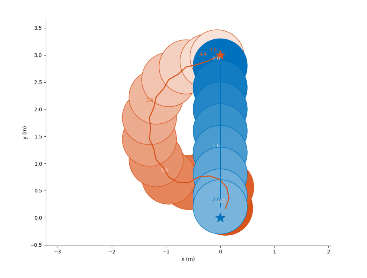
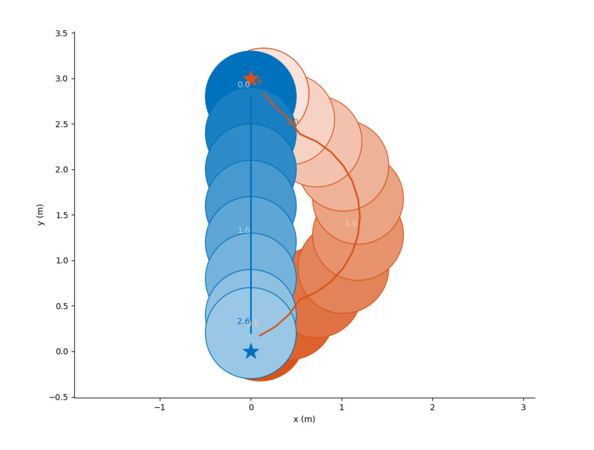
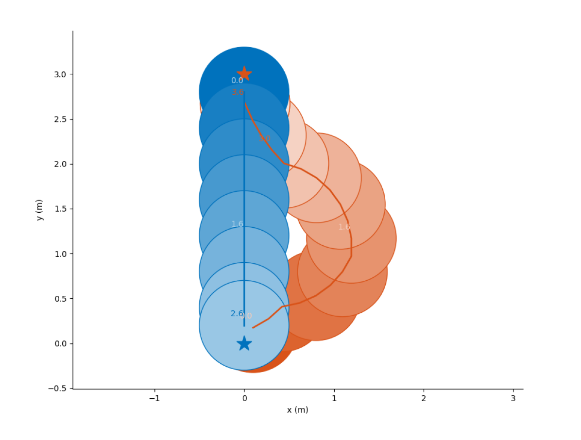
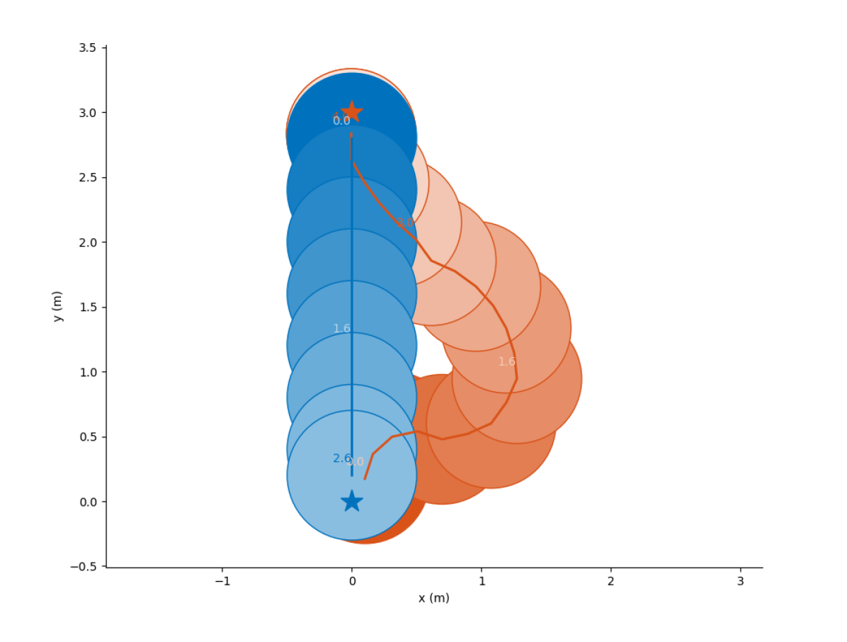
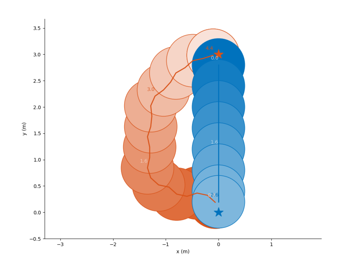
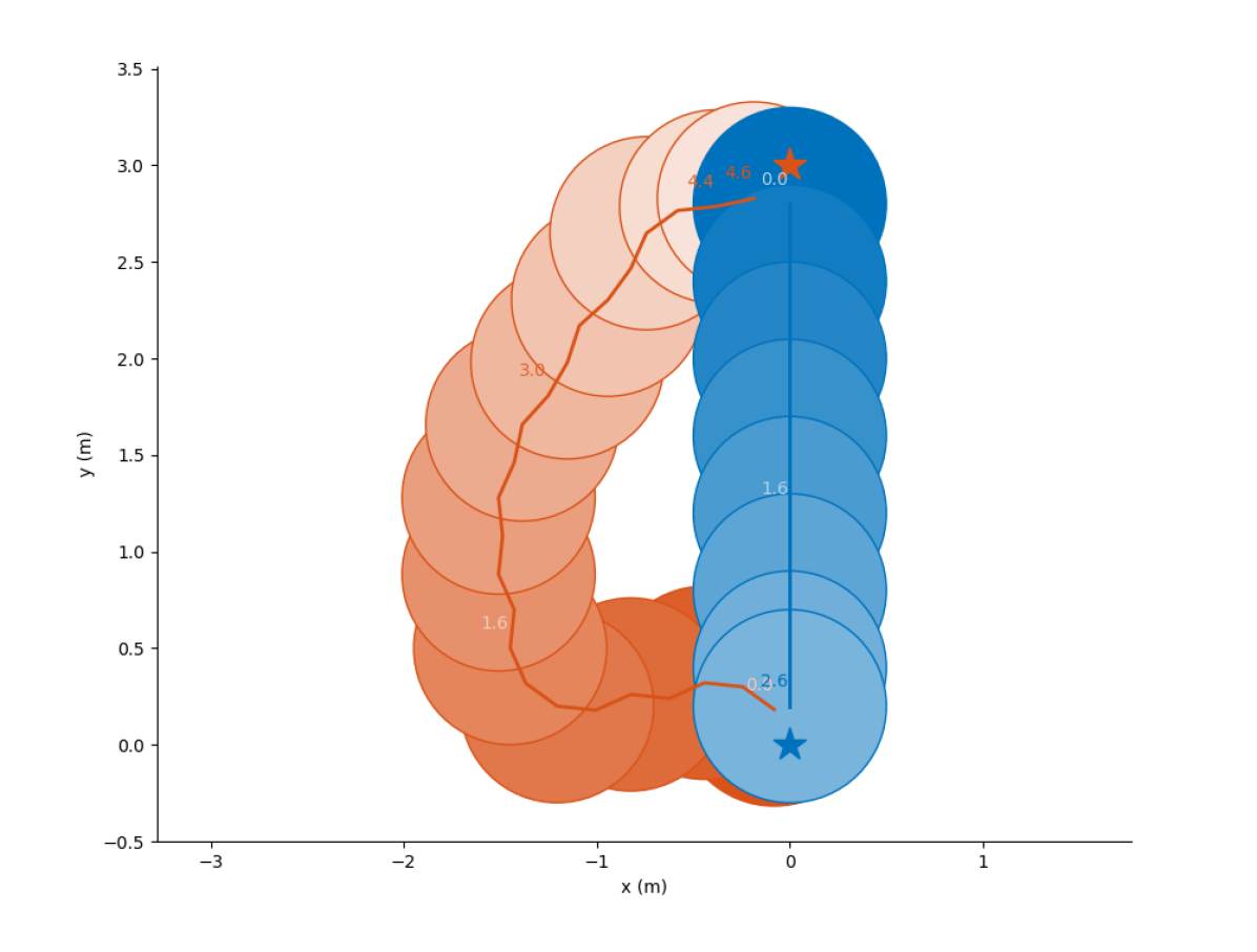
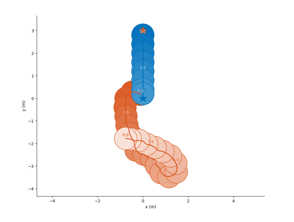
The non-dueling DQN used $2$, $64$-unit layers with hyperparameters: learning rate $2.05\texttt{e}{-4}$, $\epsilon$-greedy exploration frac. $0.497$, final $\epsilon$-greedy $0.054852$, buffer size $152\texttt{e}3$, $4\texttt{e}5$ training steps, and target network update frequency, $10\texttt{e}3$. The hyperparameters were found by running 100 iterations of Bayesian optimization with Gaussian Processes [50] on the maximization of the training reward.

5.2 Generalization to the cartpole domain

Experiments in cartpole [51] show that the increased robustness to noise can generalize to another domain. The reward is the time that a pole is successfully balanced (capped at $200$ steps). The reward of a nominal DQN drops from $199$ to $141$ under uniform noise with $\sigma{=}.25$ added to all observations. CARRL, however, considers the worst-case state, i.e., a state in which the pole is the closest to falling, resulting in a policy that recovers a reward of $180$ with $\epsilon{=}.05$, under the same noise conditions. Hyperparameters for a $2$-layer, $4$-unit network were found via Bayesian Optimization.

6 Conclusion

This work adapted deep RL algorithms for application in safety-critical domains, by proposing an add-on certified defense to address existing failures under adversarially perturbed observations and sensor noise. The proposed extension of robustness certification tools from computer vision into a deep RL formulation enabled efficient calculation of a lower bound on Q-values, given the observation uncertainty. These guaranteed lower bounds were used to modify the action selection rule to provide maximum performance under worst-case observation perturbations. The resulting policy (added onto trained DQN networks) was shown to improve robustness to adversaries and sensor noise, causing fewer collisions in a collision avoidance domain and higher reward in cartpole. Future work will extend the guarantees to continuous action spaces and experiment with robotic hardware.

Acknowledgments

This work is supported by Ford Motor Company. The computation is supported by Amazon Web Services. The authors greatly thank Tsui-Wei (Lily) Weng for providing code for the Fast-Lin algorithm and insightful discussions.

References

- Gu et al. [2017] S. Gu, E. Holly, T. Lillicrap, and S. Levine. Deep reinforcement learning for robotic manipulation with asynchronous off-policy updates. In 2017 IEEE International Conference on Robotics and Automation (ICRA), May 2017.
- Fan et al. [2019] T. Fan, X. Cheng, J. Pan, P. Long, W. Liu, R. Yang, and D. Manocha. Getting robots unfrozen and unlost in dense pedestrian crowds. IEEE Robotics and Automation Letters, 4(2):1178–1185, 2019.
- Everett et al. [2018] M. Everett, Y. F. Chen, and J. P. How. Motion planning among dynamic, decision-making agents with deep reinforcement learning. CoRR, abs/1805.01956, 2018.
- Szegedy et al. [2014] C. Szegedy, W. Zaremba, I. Sutskever, J. Bruna, D. Erhan, I. Goodfellow, and R. Fergus. Intriguing properties of neural networks. In International Conference on Learning Representations, 2014.
- Akhtar and Mian [2018] N. Akhtar and A. S. Mian. Threat of adversarial attacks on deep learning in computer vision: A survey. IEEE Access, 6:14410–14430, 2018.
- Yuan et al. [2019] X. Yuan, P. He, Q. Zhu, R. R. Bhat, and X. Li. Adversarial examples: Attacks and defenses for deep learning. IEEE transactions on neural networks and learning systems, 2019.
- Kurakin et al. [2017] A. Kurakin, I. J. Goodfellow, and S. Bengio. Adversarial examples in the physical world. In ICLR (Workshop). OpenReview.net, 2017.
- Sharif et al. [2016] M. Sharif, S. Bhagavatula, L. Bauer, and M. K. Reiter. Accessorize to a crime: Real and stealthy attacks on state-of-the-art face recognition. In Proceedings of the 2016 ACM SIGSAC Conference on Computer and Communications Security, pages 1528–1540, 2016.
-
Tencent Keen Security Lab [2019]
Tencent Keen Security Lab.
Experimental security research of Tesla Autopilot, 03 2019.
URL
https://keenlab.tencent.com/en/whitepapers/
Experimental_Security_Research_of_Tesla_Autopilot.pdf. - Kurakin et al. [2017] A. Kurakin, I. J. Goodfellow, and S. Bengio. Adversarial machine learning at scale. In ICLR. OpenReview.net, 2017.
- Madry et al. [2018] A. Madry, A. Makelov, L. Schmidt, D. Tsipras, and A. Vladu. Towards deep learning models resistant to adversarial attacks. In ICLR. OpenReview.net, 2018.
- Kos and Song [2017] J. Kos and D. Song. Delving into adversarial attacks on deep policies. In ICLR (Workshop). OpenReview.net, 2017.
- Papernot et al. [2016] N. Papernot, P. McDaniel, X. Wu, S. Jha, and A. Swami. Distillation as a defense to adversarial perturbations against deep neural networks. In 2016 IEEE Symposium on Security and Privacy (SP), pages 582–597, May 2016.
- Tramèr et al. [2018] F. Tramèr, A. Kurakin, N. Papernot, I. Goodfellow, D. Boneh, and P. McDaniel. Ensemble adversarial training: Attacks and defenses. In International Conference on Learning Representations, 2018. URL https://openreview.net/forum?id=rkZvSe-RZ.
- Carlini and Wagner [2017] N. Carlini and D. Wagner. Adversarial examples are not easily detected: Bypassing ten detection methods. In Proceedings of the 10th ACM Workshop on Artificial Intelligence and Security, AISec ’17, pages 3–14, New York, NY, USA, 2017. ACM. ISBN 978-1-4503-5202-4.
- He et al. [2017] W. He, J. Wei, X. Chen, N. Carlini, and D. Song. Adversarial example defenses: Ensembles of weak defenses are not strong. In Proceedings of the 11th USENIX Conference on Offensive Technologies, WOOT’17, pages 15–15, Berkeley, CA, USA, 2017. USENIX Association.
- Athalye et al. [2018] A. Athalye, N. Carlini, and D. Wagner. Obfuscated gradients give a false sense of security: Circumventing defenses to adversarial examples. In J. Dy and A. Krause, editors, Proceedings of the 35th International Conference on Machine Learning, volume 80 of Proceedings of Machine Learning Research, pages 274–283, Stockholmsmässan, Stockholm Sweden, 10–15 Jul 2018. PMLR.
- Uesato et al. [2018] J. Uesato, B. O’Donoghue, P. Kohli, and A. van den Oord. Adversarial risk and the dangers of evaluating against weak attacks. In J. Dy and A. Krause, editors, Proceedings of the 35th International Conference on Machine Learning, volume 80 of Proceedings of Machine Learning Research, pages 5025–5034, Stockholmsmässan, Stockholm Sweden, 10–15 Jul 2018. PMLR.
- Katz et al. [2017] G. Katz, C. W. Barrett, D. L. Dill, K. Julian, and M. J. Kochenderfer. Reluplex: An efficient SMT solver for verifying deep neural networks. In Computer Aided Verification - 29th International Conference, CAV 2017, Heidelberg, Germany, July 24-28, 2017, Proceedings, Part I, pages 97–117, 2017.
- Lomuscio and Maganti [2017] A. Lomuscio and L. Maganti. An approach to reachability analysis for feed-forward relu neural networks. CoRR, abs/1706.07351, 2017. URL http://arxiv.org/abs/1706.07351.
- Tjeng et al. [2019] V. Tjeng, K. Y. Xiao, and R. Tedrake. Evaluating robustness of neural networks with mixed integer programming. In International Conference on Learning Representations, 2019.
- Ehlers [2017] R. Ehlers. Formal verification of piece-wise linear feed-forward neural networks. In ATVA, 2017.
- Huang et al. [2017] X. Huang, M. Kwiatkowska, S. Wang, and M. Wu. Safety verification of deep neural networks. In R. Majumdar and V. Kunčak, editors, Computer Aided Verification, pages 3–29, Cham, 2017. Springer International Publishing. ISBN 978-3-319-63387-9.
- Raghunathan et al. [2018] A. Raghunathan, J. Steinhardt, and P. Liang. Certified defenses against adversarial examples. In International Conference on Learning Representations, 2018.
- [25] E. Wong and J. Z. Kolter. Provable defenses against adversarial examples via the convex outer adversarial polytope. In ICML, volume 80 of Proceedings of Machine Learning Research, pages 5283–5292.
- Weng et al. [2018] T. Weng, H. Zhang, H. Chen, Z. Song, C. Hsieh, L. Daniel, D. Boning, and I. Dhillon. Towards fast computation of certified robustness for relu networks. In ICML, 2018.
- Singh et al. [2018] G. Singh, T. Gehr, M. Mirman, M. Püschel, and M. Vechev. Fast and effective robustness certification. In Advances in Neural Information Processing Systems 31, pages 10802–10813. 2018.
- Wang et al. [2018] S. Wang, K. Pei, J. Whitehouse, J. Yang, and S. Jana. Efficient formal safety analysis of neural networks. In Advances in Neural Information Processing Systems 31, pages 6367–6377. 2018.
- Zhang et al. [2018] H. Zhang, T.-W. Weng, P.-Y. Chen, C.-J. Hsieh, and L. Daniel. Efficient neural network robustness certification with general activation functions. In S. Bengio, H. Wallach, H. Larochelle, K. Grauman, N. Cesa-Bianchi, and R. Garnett, editors, Advances in Neural Information Processing Systems 31, pages 4939–4948. Curran Associates, Inc., 2018.
- Boopathy et al. [2019] A. Boopathy, T.-W. Weng, P.-Y. Chen, S. Liu, and L. Daniel. Cnn-cert: An efficient framework for certifying robustness of convolutional neural networks. In AAAI, Jan 2019.
- Rajeswaran et al. [2017] A. Rajeswaran, S. Ghotra, B. Ravindran, and S. Levine. Epopt: Learning robust neural network policies using model ensembles. In ICLR. OpenReview.net, 2017.
- Muratore et al. [2018] F. Muratore, F. Treede, M. Gienger, and J. Peters. Domain randomization for simulation-based policy optimization with transferability assessment. In 2nd Annual Conference on Robot Learning, CoRL 2018, Zürich, Switzerland, 29-31 October 2018, Proceedings, pages 700–713, 2018.
- Uther and Veloso [1997] W. Uther and M. Veloso. Adversarial reinforcement learning. Technical report, In Proceedings of the AAAI Fall Symposium on Model Directed Autonomous Systems, 1997.
- Pinto et al. [2017] L. Pinto, J. Davidson, R. Sukthankar, and A. Gupta. Robust adversarial reinforcement learning. In D. Precup and Y. W. Teh, editors, Proceedings of the 34th International Conference on Machine Learning, volume 70 of Proceedings of Machine Learning Research, pages 2817–2826, International Convention Centre, Sydney, Australia, 06–11 Aug 2017. PMLR.
- Goodfellow et al. [2015] I. Goodfellow, J. Shlens, and C. Szegedy. Explaining and harnessing adversarial examples. In International Conference on Learning Representations, 2015.
- Xu et al. [2018] W. Xu, D. Evans, and Y. Qi. Feature squeezing: Detecting adversarial examples in deep neural networks. In NDSS. The Internet Society, 2018.
- Gehr et al. [2018] T. Gehr, M. Mirman, D. Drachsler-Cohen, P. Tsankov, S. Chaudhuri, and M. Vechev. Ai2: Safety and robustness certification of neural networks with abstract interpretation. In 2018 IEEE Symposium on Security and Privacy (SP), pages 3–18, May 2018.
- García and Fernández [2015] J. García and F. Fernández. A comprehensive survey on safe reinforcement learning. Journal of Machine Learning Research, 16:1437–1480, 2015.
- Heger [1994] M. Heger. Consideration of risk in reinforcement learning. In W. W. Cohen and H. Hirsh, editors, Machine Learning Proceedings 1994, pages 105 – 111. Morgan Kaufmann, San Francisco (CA), 1994. ISBN 978-1-55860-335-6.
- Tamar [2015] A. Tamar. Risk-sensitive and Efficient Reinforcement Learning Algorithms. PhD thesis, Technion - Israel Institute of Technology, Faculty of Electrical Engineering, 2015.
- Geibel [2006] P. Geibel. Risk-Sensitive Approaches for Reinforcement Learning. PhD thesis, University of Osnabrück, 2006.
- Fischer et al. [2019] M. Fischer, M. Mirman, S. Stalder, and M. Vechev. Online Robustness Training for Deep Reinforcement Learning. arXiv e-prints, Nov 2019.
- Kahn et al. [2017] G. Kahn, A. Villaflor, V. Pong, P. Abbeel, and S. Levine. Uncertainty-aware reinforcement learning for collision avoidance. CoRR, abs/1702.01182, 2017.
- Lütjens et al. [2019] B. Lütjens, M. Everett, and J. P. How. Safe Reinforcement Learning with Model Uncertainty Estimates. 2019 IEEE International Conference on Robotics and Automation (ICRA), May 2019.
- Sun et al. [2017] W. Sun, A. Venkatraman, G. J. Gordon, B. Boots, and J. A. Bagnell. Deeply AggreVaTeD: Differentiable imitation learning for sequential prediction. In D. Precup and Y. W. Teh, editors, Proceedings of the 34th International Conference on Machine Learning, volume 70 of Proceedings of Machine Learning Research, pages 3309–3318, International Convention Centre, Sydney, Australia, 06–11 Aug 2017. PMLR.
- Berkenkamp et al. [2017] F. Berkenkamp, M. Turchetta, A. Schoellig, and A. Krause. Safe model-based reinforcement learning with stability guarantees. In I. Guyon, U. V. Luxburg, S. Bengio, H. Wallach, R. Fergus, S. Vishwanathan, and R. Garnett, editors, Advances in Neural Information Processing Systems 30, pages 908–918. Curran Associates, Inc., 2017.
- van den Berg et al. [2009] J. P. van den Berg, S. J. Guy, M. C. Lin, and D. Manocha. Reciprocal n-body collision avoidance. In ISRR, 2009.
- Mnih et al. [2015] V. Mnih, K. Kavukcuoglu, D. Silver, A. A. Rusu, J. Veness, M. G. Bellemare, A. Graves, M. Riedmiller, A. K. Fidjeland, G. Ostrovski, S. Petersen, C. Beattie, A. Sadik, I. Antonoglou, H. King, D. Kumaran, D. Wierstra, S. Legg, and D. Hassabis. Human-level control through deep reinforcement learning. In Nature, volume 518. Nature Publishing Group, a division of Macmillan Publishers Limited., 2015.
- Trautman and Krause [2010] P. Trautman and A. Krause. Unfreezing the robot: Navigation in dense, interacting crowds. In 2010 IEEE/RSJ International Conference on Intelligent Robots and Systems, pages 797–803, Oct 2010.
- Snoek et al. [2012] J. Snoek, H. Larochelle, and R. P. Adams. Practical bayesian optimization of machine learning algorithms. In F. Pereira, C. J. C. Burges, L. Bottou, and K. Q. Weinberger, editors, Advances in Neural Information Processing Systems 25, pages 2951–2959. Curran Associates, Inc., 2012.
- Barto et al. [1983] A. G. Barto, R. S. Sutton, and C. W. Anderson. Neuronlike adaptive elements that can solve difficult learning control problems. IEEE transactions on systems, man, and cybernetics, (5):834–846, 1983.