“Please come back later”: Benefiting from deferrals in service systems

Abstract

The performance evaluation of loss service systems, where customers who cannot be served upon arrival get dropped, has a long history going back to the classical Erlang B model. In this paper, we consider the performance benefits arising from the possibility of deferring customers who cannot be served upon arrival. Specifically, we consider an Erlang B type loss system where the system operator can, subject to certain constraints, ask a customer arriving when all servers are busy, to come back at a specified time in the future. If the system is still fully loaded when the deferred customer returns, she gets dropped for good. For such a system, we ask: How should the system operator determine the ‘rearrival’ times of the deferred customers based on the state of the system (which includes those customers already deferred and yet to arrive)? How does one quantify the performance benefit of such a deferral policy?

Our contributions are as follows. We propose a simple state-dependent policy for determining the rearrival times of deferred customers. For this policy, we characterize the long run fraction of customers dropped. We also analyse a relaxation where the deferral times are bounded in expectation. Via extensive numerical evaluations, we demonstrate the superiority of the proposed state-dependent policies over naive state-independent deferral policies.

I Introduction

Many service systems have the property that denial of service upon the arrival of a request results in the request getting dropped. The classical example comes from telephony, where an incoming call request must either be connected, or dropped. Another contemporary example is an electric car charging facility, which cannot serve an incoming customer when all charging stations are occupied. Similarly, certain online services decline fresh requests when congested.

Such service systems, by their very nature, are unable to queue requests that arrive when service capacity is fully utilized. It is therefore natural to ask: What if these systems were instead able to defer some requests, i.e., have these requests ‘come back’ at a pre-specified time in the future? If so, what is optimal strategy for deferring requests? To what extent does the throughput of the system improve from such a deferral policy? The goal of this paper is to shed light on these questions.

Formally, we consider an Erlang B (M/M/$K$/$K$) service system, where the system operator can, subject to certain constraints, defer jobs that arrive when all servers are occupied. The constraints include an upper bound on the deferral time (which is natural given QoS considerations), and/or a constraint on the number of jobs that can be deferred at any time. In this setting, our goal is to design simple deferral policies that are effective, while also being analytically tractable. The main difficulty in the performance evaluation of deferral policies is that the state description must incorporate information about (future) arrival instants of deferred jobs.

Our main contribution is the design and analysis of a deferral policy, which spaces arrivals of deferred jobs uniformly in the future. Even though this policy induces a complicated (uncountable) Markovian state space, we are able to analytically characterize the blocking probability via a novel combination of steady state and transient analysis of certain Markov processes. Via numerical experiments, we show that the proposed policy outperforms naive state-independent deferral policies, as well as the Erlang B system (which does not allow deferrals).

A relaxation on the deferral time constraint is considered next, where the upper bound on the deferral time is imposed in expectation. For this relaxed model, we propose a deferral policy, which admits a considerably more explicit performance characterization. Via numerical experiments, we show that the performance of this policy is in fact a good approximation to the policy designed for the ‘hard’ deferral constraint.

The remainder of the paper is as follows. We provide a brief survey of related literature next. In Section II, we describe the primary system model and state some preliminary results. The ‘hard’ case where deferral times are bounded deterministically is considered in Section III, and the relaxed model is considered in Section IV.

Related literature: This work is motivated by the recent work [3], which implemented a deferral system for a web-server that is prone to congestion. To the best of our knowledge, there is no prior work that provides an analytical treatment of queueing systems that allow deferral.

This work is peripherally related to the considerable literature on retrial queues (we refer the reader to a recent survey paper [6] and the book [1]). Retrial queues are systems where blocked customers ‘try again later’. The main contrast between retrial queues and deferral queues is that in the former setting, the retrial model is taken to be exogenous and indicative of customer behavior, while in the latter setting, deferral is a control decision on part of the system operator.

Another related class of loss systems that have been studied are abandonment based queues (references include [2] and [7]). In these systems, customers who are denied service upon arrival wait for a certain (potentially random) amount of time. If service is not offered before this patience time runs out, the customer leaves. In contrast, in deferral queues, a deferred customer does not actually wait, but rather leaves the system to come back at a pre-specified time. So this deferred customer can only be served if service capacity is available at the precise moment of re-entry. In this sense, abandonment based systems provide lower bounds on the performance achievable in deferral systems.

II Model and Preliminaries

We consider a loss service system consisting of $K$ identical parallel servers of unit speed. Jobs (or customers) arrive according to a Poisson process of rate $\lambda,$ and service times are exponentially distributed with rate $\mu.$ In the absence of deferrals, this system is the classical Erlang B (M/M/$K$/$K$) queue.

On this baseline Erlang B model, we allow the system operator (or the scheduling policy) to defer jobs that arrive when all servers are busy, to come back to the system at a pre-specified time in the future. If a free server is available when this deferred job comes back, it gets admitted into service. If not, the job gets dropped. In other words, we only allow a job to be deferred once. We refer to the time instant at which a deferred job comes back to the system as its rearrival time, and we refer to the interval between the rearrival time and the original arrival time as the deferral time.

Of course, it is natural to impose certain constraints on the deferral policy. Firstly, QoS considerations dictate that deferral time cannot be too large. We impose this constraint in two ways: In Section III, we consider the case where there is a deterministic upper bound $\hat{T}>0$ on deferral times. In Section IV, we consider a relaxed model where the deferral times are bounded above in expectation by $\hat{T}.$ A second constraint we impose is an upper bound $\hat{D}$ on the number of deferred jobs at any time. Finally, we impose work conservation, i.e., when a job arrives (either for the first time, or post deferral), it must be served so long as there is at least one free server available.

Our metric for evaluating the performance of a deferral policy is the long run fraction of jobs blocked, a.k.a., the blocking probability. Note that jobs can be blocked in two ways: One, a job arrives when all servers are busy, and there are already $\hat{D}$ previous arrivals that have been scheduled for rearrival in the future. Second, a deferred job on rearrival finds that all the servers are (still) busy.

A naive deferral policy would be to assign a large deferral time (say $\hat{T}$), subject to limit $\hat{D}$ on number of deferred jobs. Another naive policy would be to assign a deferral time sampled uniformly at random in $[0,\hat{T}],$ again subject to the deferral limit. Such policies are state-independent, in that the deferral time of a job is assigned independently of the deferral times assigned to previous jobs. In this paper, we propose low overhead state-dependent deferral policies, that schedule rearrivals of deferred jobs cognizant of the already scheduled rearrivals.

Finally, we note that work conservation ensures that the blocking probability of any deferral policy is at most the blocking probability in the Erlang B system. In other words, the Erlang B formula provides an upper bound on the blocking probability of any deferral policy.

Throughout the paper, for $n\in\mathbb{N},$ the set $\{0,1,2,\cdots,n\}$ is denoted by $[n].$

III Bounded Deferral Times

In this section, we consider the case where the deferral times are bounded by $\hat{T}>0,$ i.e., the system cannot defer an incoming job by more than $\hat{T}$ time units. For this model, we propose a simple state-dependent deferral policy, which we refer to as the Determinstically Spaced Rearrival Times (DSRT) policy, which spreads the rearrival instants of deferred jobs ‘uniformly’, so as to maximize the chances of admitting them. We provide a characterization of the blocking probability under this policy, via a novel combination of the steady state analysis of a Markov chain that captures the system evolution in the absence of deferrals, and the transient analysis of another Markov chain that captures the system evolution in the presence of deferrals. Finally, we present a case study that demonstrates the superiority of our state-dependent deferral policy over naive state-independent policies.

III-A DSRT Policy

The proposed deferral policy is described as follows. It is parameterized by $x\in(0,\hat{T}],$ which specifies the spacing between arrivals of deferred jobs into the system. If there are no jobs currently deferred, and an arriving job finds all servers busy, then the policy defers that job by $x$ time units. On the other hand, if there are deferred jobs, and an arriving job finds all servers busy, then the policy schedules its rearrival time to be $x$ time units after the rearrival time of the last deferred job, subject to a maximum of $D=\min(\hat{D},\left\lfloor\hat{T}/x\right\rfloor)$ deferred jobs at any time. This policy is defined formally as Algorithm 1.

Algorithm 1 DSRT policy

procedure DSRT

     if $\text{num\_deferrals}=0$ then

         $\text{rearrival\_time}\leftarrow\text{arrival\_time}+x$

     else if $\text{num\_deferrals}<D:=\min(\hat{D},\left\lfloor\hat{T}/x\right\rfloor)$ then

         $\text{rearrival\_time}\leftarrow\text{prev\_rearrival\_time}+x$

     else

         Customer blocked

     end if

end procedure

Note that the proposed DSRT policy attempts to spread the rearrival instants $x$ units of time apart, subject to the deferral constraints. Intuitively, if the spacing $x$ is too small, then the deferred jobs are likely to find all servers occupied upon rearrival. On the other hand, if $x$ is too large, the policy is inefficient, since fewer jobs may be deferred at any time (given the constraint $\hat{T}$ on the deferral times), and fewer opportunities are created to admit deferred jobs. Thus, the policy must operate at an intermediate ‘soft spot’; we address this issue in our numerical experiments.

Under the DSRT policy, the temporal evolution of the system can be captured as a Markov process over state space $[K]\times[D]\times[0,x].$ Here, the state $(k,d,\theta)$ indicates that $k$ servers are currently busy, there are $d$ jobs in deferral, and that the earliest rearrival of a deferred job will occur after time $\theta.$ Note that the state space is uncountable, making an analysis of the stationary distribution cumbersome. We overcome this difficulty by directly characterizing $\Pi_{k,d}$ which is the long run fraction of time the state is of the form $(k,d,\theta)$ for some $\theta\in[0,x].$ This is done by separately analysing the temporal evolution of the system in the presence and absence of deferred jobs, and then combining these analyses in a novel manner.

We begin by considering the special case of a single server, and a limit of at most one deferral at any time ($K=D=1$). This special case is instructive, not just because it illustrates our analysis approach, but also because it admits a closed form characterization of the blocking probability. We then consider the case of general $K,$ $D$ in Section III-C; in this case, our characterization is less explicit, though amenable to an exact computation.

III-B Single-Server, Single-Deferral System

Figure 1: Illustration of the temporal evolution of $\theta$ when $K=D=1.$ Deferral phases ($d>0$) of length $x$ are interspaced between non-deferral phases ($d=0$).

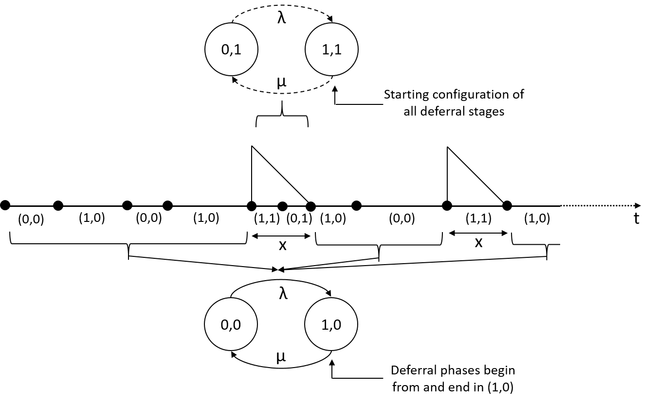
The temporal evolution of the system for the case $K=D=1$ is illustrated in Figure 1. The key observation that informs our analysis is the following. Considering only the times when the system has no deferrals (i.e., disregarding the deferral phases, when $d>0$), the system configuration evolves as per the Markov chain depicted at the bottom of Figure 1. On the other hand, over each deferral phase of length $x$ (when $d>1$) the system configuration evolves as per the Markov chain depicted at the top of Figure 1.

Since the system configuration evolves as per the Markov chain depicted at the bottom of Figure 1 when there are no deferrals, the ratio between $\Pi_{0,0}$ and $\Pi_{1,0}$ is dictated by the flow balance equations for that Markov chain:

$$\lambda\Pi_{0,0}=\mu\Pi_{1,0}.$$ (1)

Turning now to the configurations where $d=1,$ we note that the relationship between $\Pi_{0,1}$ and $\Pi_{1,1}$ is dictated by the transient behavior of the Markov chain depicted on the top of Figure 1 over an interval of length $x,$ starting in configuration $(1,1).$ Focusing on this Markov chain over the interval $[0,x],$ the distribution of the chain at time $t,$ captured by $\textbf{p}(t)=[p_{0,1}(t),p_{1,1}(t)],$ is given by:

$$\textbf{p}(t)=[0,1]e^{Qt},$$

where

$$Q=\begin{bmatrix}-\lambda&\lambda\\ \mu&-\mu\end{bmatrix}.$$

It now follows that

$$\frac{\Pi_{0,1}}{\Pi_{1,1}}=\frac{\int_{0}^{x}p_{0,1}(t)dt}{\int_{0}^{x}p_{1,1}(t)dt}.$$ (2)

Next, we need to relate the long run fraction of time spent in non-deferral configurations $(d=0)$ to those under deferral configurations $(d=1)$. To do this, we note, using the PASTA property, that the rate at which transitions occur from non-deferral configurations to deferral configurations equals $\lambda\Pi_{1,0}.$ On the other hand, transitions from deferral configurations to non-deferral configurations occur at rate $\frac{\Pi_{0,1}+\Pi_{1,1}}{x}.$ Equating the two, we get:

$$\lambda\Pi_{1,0}=\frac{\Pi_{0,1}+\Pi_{1,1}}{x}.$$ (3)

Lastly, we have the normalization condition

$$\Pi_{0,0}+\Pi_{1,0}+\Pi_{0,1}+\Pi_{1,1}=1.$$ (4)

Solving the system of equations (1)–(4) gives yields a closed form characterization of the long run fraction of time spent in each configuration.

Figure 2: Illustration of the temporal evolution of $\theta$ when $K=2,D=3.$

Figure 3: System evolution over the non-deferral configurations

Figure 4: System evolution within each deferral stage

Finally, we are interested in characterizing the blocking probability $P_{B},$ which is the long run fraction of customers dropped. This can be done as follows:

$$P_{B}=\Pi_{1,1}+\frac{(\Pi_{0,1}+\Pi_{1,1})p_{1,1}(x)}{\lambda x}$$ (5)

The first term above captures the long run fraction of customers dropped on arrival (because the server was busy and there was already a deferred customer). The second term captures the long run fraction of customers dropped post deferral on rearrival. Indeed, the probability that any deferred customer gets dropped on rearrival equals $p_{1,1}(x).$ Thus, the rate of drops of deferred customers equals $\frac{(\Pi_{0,1}+\Pi_{1,1})p_{1,1}(x)}{x}.$

To summarize, solving equations (1)–(4), and applying the solution to (5) yields the following result.

Theorem 1

For the case $K=D=1,$ under the DSRT policy, the blocking probability $P_{B}$ is given by

$$\text{P}_{B}=\frac{\rho}{1+\rho}-\frac{\rho(1-\text{exp}\{-(\lambda+\mu)x\})}{(1+\rho)^{2}(1+\rho(1+\lambda x))},$$ (6)

where $\rho:=\lambda/\mu$.

Note that $\frac{\rho}{1+\rho}$ is the blocking probability of an M/M/1/1 system. It is therefore clear from (6) that the blocking probability under the DSRT policy is a strict improvement over the scenario where deferral is not allowed. Moreover, the improvement diminishes to zero when $x=0$ and as $x\rightarrow\infty.$ While the optimal value of $x$ that minimizes $P_{B}$ does not admit an explicit formula, it can be shown that the optimal value is bounded between $\frac{1}{\lambda+\mu}$ and $\frac{\sqrt{2}}{\lambda}$.

III-C Multiple-Servers, Multiple-Deferrals System

We now turn to the performance evaluation in the general setting, i.e., the number of servers $K$ and the maximum number of deferrals $D$ are arbitrary. Figure 2 illustrates the temporal evolution of $\theta$ in this case. Note that each deferral phase (an interval over which $d>0$) is no longer necessarily of duration $x$ anymore, but is instead made up of a random number of deferral stages, each of duration $x.$ Moreover, at the end of each deferral phase, the configuration is of the form $(k,0)$ where $0<k\leq K.$ Thus, disregarding the deferral phases, the system configuration evolves as per the Markov chain depicted in Figure 3. Here, $\alpha_{i}$ denotes the probability that a deferral phase ends with $i$ active servers. (The values of $\alpha_{i}$ are in turn dictated by the behavior of the system during each deferral phase; we will characterize $\alpha_{i}$ shortly.) Moreover, over each deferral stage of duration $x,$ the system configuration evolves as per the Markov chain shown in Figure 4.

In order to characterize $\alpha_{i},$ and to arrive at the system of equations relating the long run fractions of time spent in the different configurations, we first analyse the evolution of the system configuration over a single deferral stage, and then consider the sequence of starting configurations across deferral stages within a deferral phase.

III-C1 Evolution of system configuration within a single deferral stage

Deferral stages begin in a configuration of the form $(k,d),$ where $1\leq k\leq K,$ and $1\leq d<D.$ Subsequently for duration $x,$ the system configuration evolves as per the Markov chain depicted in Figure 4. The transition rate matrix corresponding to this chain is given by

$$Q=\begin{bmatrix}Q_{1}&\Lambda&\textbf{0}&\textbf{0}&\ldots&\textbf{0}\\ \textbf{0}&Q_{1}&\Lambda&\textbf{0}&\ldots&\textbf{0}\\ \textbf{0}&\textbf{0}&\ddots&\ddots&&\textbf{0}\\ \textbf{0}&\textbf{0}&&\ddots&\ddots&\textbf{0}\\ \textbf{0}&\textbf{0}&\ldots&\textbf{0}&Q_{1}&\Lambda\\ \textbf{0}&\textbf{0}&\textbf{0}&\ldots&\textbf{0}&Q_{2}\end{bmatrix},$$

where 0 is an all-zero square matrix of size $(K+1)$, $Q_{2}$ is the transition rate matrix of an M/M/K/K queue, $\Lambda$ is a diagonal matrix with entries $(0,\cdots,0,\lambda)$, and $Q_{1}=Q_{2}-\Lambda$. In writing this rate matrix, the configurations $(k,d)$ have been ordered by stacking them row-wise from Figure 4.

Considering the evolution of this chain over the interval $[0,x],$ the distribution at time $t$ is denoted by the vector $\textbf{p}(t),$ where

$$\textbf{p}(t)=\textbf{p}_{\text{init}}e^{Qt}.$$

Here, the initial probability vector $\textbf{p}_{\text{init}}$ would have an entry 1 according to the starting configuration of the stage under consideration, the other entries being zero.

III-C2 Evolution of deferral stage starting configurations

As mentioned before, the starting configuration in a deferral stage is of the form $(k,d),$ where $1\leq k\leq K,$ and $1\leq d<D.$ We construct a discrete time Markov chain to capture the evolution of the starting configurations across successive deferral stages. To make the chain recurrent, we add a dummy state $\mathcal{D}$ which captures the end of the deferral phase. Note that the transition from the dummy state is to the configuration $(K,1),$ since that is the starting configuration on the next deferral phase.

To describe the transition probability matrix corresponding to this discrete time Markov chain, we need the following notation. Within a deferral stage, let $p_{k^{\prime},d^{\prime}}^{k,d}(t)$ denote the probability of being in configuration $(k^{\prime},d^{\prime})$ at time $t\in[0,x],$ with starting configuration $(k,d).$ Note that these probabilities are defined in Section III-C1.

Now, let $\hat{p}(c^{\prime}|c)$ denote the probability that the starting configuration in the next deferral stage is $c^{\prime}$ given that the starting configuration in the present deferral stage is $c,$ where

$$c,c^{\prime}\in\hat{S}:=\{(k,d)\>1\leq k\leq K,\ 1\leq d<D\}\cup\{\mathcal{D}\}.$$

The transition probabilities $\hat{p}(\cdot|\cdot)$ are given by

$$\hat{p}((k^{\prime},d^{\prime})|(k,d)) =p_{k^{\prime}-1,d^{\prime}+1}^{k,d}(x)$$

$$\qquad\qquad\text{for }1\leq k^{\prime}<K,\ 1\leq d^{\prime}<D,$$

$$\hat{p}((K,d^{\prime})|(k,d)) =p_{K-1,d^{\prime}+1}^{k,d}(x)+p_{K,d^{\prime}+1}^{k,d}(x)$$

$$\qquad\qquad\text{for }1\leq d^{\prime}<D,$$

$$\hat{p}(\mathcal{D}|(k,d)) =\sum_{\ell=0}^{K}p_{\ell,1}^{k,d}(x),$$

$$\hat{p}((K,1)|\mathcal{D}) =1.$$

Given these transition probabilities corresponding to this finite irreducible discrete time Markov chain, one can obtain the stationary distribution. Let $P_{\text{start}}^{c}$ denote the stationary probability associated with configuration $c\in\hat{S}.$

III-C3 The equations relating $\Pi_{k,d}$

We begin by relating the long run fractions of time spent in the non-deferral configurations. This is in turn based on the Markov chain depicted in Figure 3. The probabilities $\alpha_{l}$ are characterized as follows.

Lemma 1

For $1\leq l<K,$

$$\alpha_{l}=\frac{\sum_{j=1}^{k}P_{\text{start}}^{j,1}~{}p_{l-1,1}^{j,1}(x)}{\sum_{j=1}^{k}P_{\text{start}}^{j,1}~{}\sum_{l^{\prime}=0}^{k}p_{l^{\prime},1}^{j,1}(x)}.$$

Proof:

The characterization of $\alpha_{l}$ follows directly from the discrete-time Markov chain discussed in Section III-C2; indeed, $\alpha_{l}$ is simply the probability that a deferral phase ends with a transition to the configuration $(l,0).$ Consider a (discrete-time) renewal process where renewal instance correspond to visits to the dummy state (i.e., the end of a deferral phase) in the above DTMC. Each renewal cycle produces a reward of 1 if it ends with a transition to the configuration $(l,0),$ and zero otherwise. An application of the renewal reward theorem yields

$$\sum_{j=1}^{k}P_{\text{start}}^{j,1}~{}p_{l-1,1}^{j,1}(x)=\alpha_{l}P_{\text{start}}^{\mathcal{D}}.$$

The statement of the lemma now follows, once we note that the balance equations for the DTMC under consideration imply

$$P_{\text{start}}^{\mathcal{D}}=\sum_{j=1}^{k}P_{\text{start}}^{j,1}~{}\sum_{l^{\prime}=0}^{k}p_{l^{\prime},1}^{j,1}(x).$$

∎

Given this result, we have:

$$\begin{array}[]{rl}\lambda\Pi_{0,0}&=\mu\Pi_{1,0},\\ (\lambda+l\mu)\Pi_{l,0}&=\lambda\Pi_{l-1,0}+(l+1)\mu\Pi_{l+1,0}+\lambda\alpha_{l}\Pi_{K,0},\\ &\qquad\qquad\text{ for }(1\leq l<K).\end{array}$$ (7)

Next, we focus on the ratio of long run fraction of time spent in deferral configurations. This is given by

$$\frac{\Pi_{k_{1},d_{1}}}{\Pi_{k_{2},d_{2}}} =\frac{\sum_{k=1}^{K}\sum_{d=1}^{D-1}P_{\text{start}}^{k,d}\int_{0}^{x}p_{k_{1},d_{1}}^{k,d}(t)\text{d}t}{\sum_{k=1}^{K}\sum_{d=1}^{D-1}P_{\text{start}}^{k,d}\int_{0}^{x}p_{k_{2},d_{2}}^{k,d}(t)\text{d}t},$$ (8)

where $0\leq k_{1},k_{2}\leq K$ and $1\leq d_{1},d_{2}\leq D$.

Finally, it remains to relate the time fractions corresponding to deferral configurations to those corresponding to non-deferral configurations. This is done as follows:

$$\lambda\Pi_{K,0}=\frac{(\sum_{k=0}^{K}\sum_{d=1}^{D}\Pi_{k,d})(~{}\sum_{j=1}^{K}P_{\text{start}}^{j,1}~{}\sum_{l=0}^{K}p_{l,1}^{j,1}(x)~{})}{x(1-P_{\text{start}}^{\mathcal{D}})}.$$ (9)

This is justified as follows. $\lambda\Pi_{K,0}$ gives the rate of transition from non-deferral configurations to deferral configurations. On the other hand, the rate of rearrivals equals $\frac{\sum_{k=0}^{K}\sum_{d=1}^{D}\Pi_{k,d}}{x}.$ $\frac{\sum_{j=1}^{K}P_{\text{start}}^{j,1}~{}\sum_{l=0}^{K}p_{l,1}^{j,1}(x)}{1-P_{\text{start}}^{\mathcal{D}}}$ gives the probability of exiting the positive deferral configurations at the end of any deferral stage of duration $x$ . (9) follows by combining these arguments.

Solving the system of linear equations (7)–(9) along with the normalization condition yields $\Pi_{k,d}$ for $(k,d)\in[K]\times[D].$

III-C4 Blocking probability characterization

The blocking probability can be characterized in a similar manner as before.

Lemma 2

Under the DSRT policy,

$$P_{B}=\Pi_{K,D}+\Pi_{K,0}\frac{\sum_{k=1}^{K}\sum_{d=1}^{D-1}P^{k,d}_{\text{start}}\sum_{l=1}^{D}p_{K,l}^{i,j}(x)}{\sum_{j=1}^{K}P_{\text{start}}^{j,1}~{}\sum_{l=0}^{K}p_{l,1}^{j,1}(x)}.$$ (10)

Proof:

Customers are blocked in two ways. First, a customer arrives when the system configuration is $(K,D).$ Using the PASTA property, the long run fraction of arrivals blocked this way equals $\Pi_{K,D},$ which accounts for the first term in (10).

Second, deferred customers can get blocked when all servers are busy upon rearrival. Let $DP(t)$ denote the number of deferral phases completed until time $t,$ and $B_{i}$ denote the number of deferred customers blocked in deferral phase $i.$ Let $A(t)$ denote the number of arrivals until time $t.$ The long run fraction of arrivals blocked upon rearrival equals

$$\lim_{t\rightarrow\infty}\frac{\sum_{i=1}^{DP(t)}B_{i}}{A(t)}$$

$$= \lim_{t\rightarrow\infty}\frac{t}{A(t)}\frac{DP(t)}{t}\frac{\sum_{i=1}^{DP(t)}B_{i}}{DP(t)}$$

$$= \frac{1}{\lambda}\left(\lambda\Pi_{K,0}\right)\mathbb{E}\left[B_{1}\right].$$

Finally, a renewal reward argument analogous to that in the proof of Lemma 1 yields

$$\mathbb{E}\left[B_{1}\right] =\frac{\sum_{k=1}^{K}\sum_{d=1}^{D-1}P^{k,d}_{\text{start}}\sum_{l=1}^{D}p_{K,l}^{i,j}(x)}{P_{\text{start}}^{\mathcal{D}}}$$

$$= \frac{\sum_{k=1}^{K}\sum_{d=1}^{D-1}P^{k,d}_{\text{start}}\sum_{l=1}^{D}p_{K,l}^{i,j}(x)}{\sum_{j=1}^{K}P_{\text{start}}^{j,1}~{}\sum_{l=0}^{K}p_{l,1}^{j,1}(x)}.$$

∎

III-D Case Study

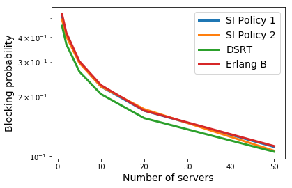
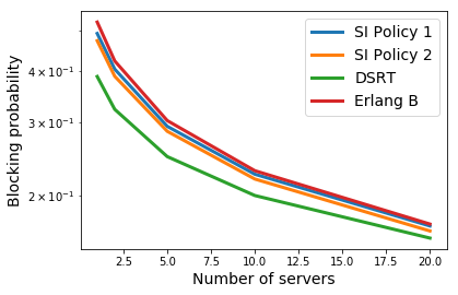
In this section, we numerically compare the performance of the DSRT policy with state-independent policies and the M/M/$K$/$K$ system in the Halfin-Whitt regime (a.k.a. quality and efficiency driven regime; see [4]). We consider two simple state independent policies: the first policy assigns a deferral time equal to $\hat{T}$ and the second policy assigns a deferral time uniformly sampled in the interval $[0,\hat{T}]$. The Halfin-Whitt regime corresponds to a sequence of queueing systems parameterized by the number of servers $K.$ The arrival rate in the system with $K$ servers equals $K+\beta\sqrt{K}$, where $\beta$ is a constant. In our experiments, the service rate for each server is set to be 1, the patience time $\hat{T}$ is set to be 10, and $\beta$ is set to be 0.1.

We compare the policies for the cases when $\hat{D}$ equals 1 and 2. We emphasize that $\hat{D}$ acts as a parameter for the state-independent policies while the deferral limit for DSRT $D=\min(\hat{D},\left\lfloor T/x\right\rfloor)$, where $x\leq T$. For DSRT, the blocking probability is evaluated numerically using the procedure developed in previous sections and is optimized by tuning the parameter $x.$ For the state independent policies, we run MCMC simulations where the blocking probability is calculated for 100,000 customers. The blocking probability for M/M/$K$/$K$ system is calculated numerically using the Erlang-B formula. The blocking probabilities of the policies for the cases where $\hat{D}$ is equal to 1 and 2 are given in Figure 5(a) and Figure 5(b) respectively. We note that DSRT outperforms the state-independent policies, which produce a blocking probability close to the Erlang-B formula.

(a) Maximum Deferrals: 1

(b) Maximum Deferrals: 2

Figure 5: Performance Evaluation

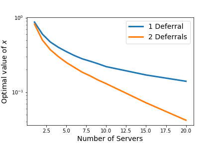
The optimal value of $x$ is plotted against the number of servers in Figure 6. Note that as the number of servers increases, the optimal value of $x$ shrinks. Characterizing this behavior analytically presents an interesting avenue for future work.

Figure 6: Optimal $x$ for DSRT

IV Deferral Times Bounded in Expectation

In this section, we consider a relaxation of the deferral constraint considered before, in that the upper bound on deferral times is imposed in expectation (rather than on each instance, as in Section III). Specifically, we require that the expected deferral time should not exceed $\hat{T}$. This relaxation may be interpreted as an approximation of the ‘hard’ deferral constraint considered before.

In the above setting, we propose and analyse a deferral policy, referred to as the Exponentially Spaced Rearrival Times (ESRT) policy. As the name suggests, this policy introduces an exponentially distributed spacing between rearrival instants. Specifically, the ESRT policy allots exponentially separated deferral times, i.e., the difference between the rearrival times of deferred arrivals is exponential with rate $\alpha$, where $1/\alpha\leq\hat{T}$, the deferral limit being $D=\min(\hat{D},\left\lfloor\hat{T}\alpha\right\rfloor);$ this policy is described formally in Algorithm 2. Note that $\text{Exp}(\alpha)$ refers to an exponential random variable with rate $\alpha$ that is independent of the workload, as well as other inter-rearrival intervals.

Algorithm 2 ESRT Policy

procedure 

     if $\text{num\_deferrals}=0$ then

         $\text{rearrival\_time}=\text{arrival\_time}+\text{Exp}(\alpha)$

     else if $0<\text{num\_deferrals}<D$ then

         $\text{rearrival\_time}=\text{prev\_rearrival\_time}+\text{Exp}(\alpha)$

     else

         customer blocked

     end if

end procedure

Given the memorylessness of the interarrival times, service times, and the time until next rearrival, the evolution of the system under the ESRT policy is described by a continuous time Markov chain over the state space $[K]\times[D],$ where state $(k,d)$ indicates that $k$ servers are currently active, and there are $d$ jobs in deferral. The transition rate diagram for this Markov chain is depicted in Figure 7. Note that memorylessness of the time until the next rearrival results in a much simpler system description (compared to the DSRT policy analysed in the previous section), and yields a much more explicit performance evaluation. In the following, we first compute the stationary distribution corresponding to the ESRT Markov chain, and then use that to characterize the blocking probability.

Figure 7: Dynamics of ESRT

IV-A Obtaining the stationary distribution

Matrix geometric methods can be used to obtain the stationary distribution corresponding to the Markov chain shown in Figure 7. Let $\Pi_{k,d}$ represent the steady state probability of state $(k,d).$

We begin by writing the flow balance equations for states with $D$ deferrals

$$(\lambda+\alpha)\Pi_{0,D}=\mu\Pi_{1,D},$$

$$(\lambda+j\mu+\alpha)\Pi_{j,D}=(j+1)\mu\Pi_{j+1,D}+\lambda\Pi_{j-1,D},$$

$$\hskip 180.67499pt\text{for }(0<j<K).$$

Letting $\vec{\Pi}_{D}:=[\Pi_{0,D},\cdots,\Pi_{K,D}]$, the above system of $K$ equations can be used to characterize $\vec{\Pi}_{D}$ upto a multiplicative constant. Specifically, we write

$$\vec{\Pi}_{D}=c\vec{V}_{D},$$ (11)

where $\vec{V}_{D}$ is a row vector whose last entry is 1.

Now, consider the collection of states corresponding to $d$ deferrals, where $d\in\{1,\cdots,D-1\}$ deferrals. The flow balance equations for these states are as follows

$$(\lambda+\alpha)\Pi_{0,d}=\mu\Pi_{1,d},$$

$$(\lambda+j\mu+\alpha)\Pi_{j,d}=(j+1)\mu\Pi_{j+1,d}+\lambda\Pi_{j-1,d}+\alpha\Pi_{j-1,d+1},$$

$$\hskip 180.67499pt\text{for }(0<j<K),$$

$$\lambda\Pi_{K,d}=\alpha\sum_{i=0}^{K}\Pi_{i,d+1}.$$

Let $\vec{\Pi}_{d}=[\Pi_{0,d},\cdots,\Pi_{K,d}]$, then the above equations can be written as

$$\vec{\Pi}_{d}A(\alpha)=\vec{\Pi}_{d+1}B(\alpha)\text{ where }$$

$$A(\alpha)=\begin{bmatrix}\lambda+\alpha&-\lambda&0&\cdots&0\\ -\mu&\lambda+\mu+\alpha&-\lambda&\cdots&0\\ 0&-2\mu&\lambda+2\mu+\alpha&\cdots&0\\ \vdots&\vdots&\ddots&\vdots&\vdots\\ 0&0&\cdots&-D\mu&\lambda\end{bmatrix}$$

and $$B(\alpha)=\begin{bmatrix}0&\alpha&0&\cdots&\alpha\\ 0&0&\alpha&\cdots&\alpha\\ 0&0&0&\cdots&\alpha\\ \vdots&\vdots&\ddots&\vdots&\vdots\\ 0&0&0&\cdots&\alpha\end{bmatrix}.$$

One can show using a simple manipulation and strict diagonal dominance that $A(\alpha)$ is non-singular. Hence, we have the following recursive relation

$$\vec{\Pi}_{d}=\vec{\Pi}_{d+1}R(\alpha)\quad\text{ for }1\leq d<D,$$ (12)

where $R(\alpha)=B(\alpha)A(\alpha)^{-1}.$

Finally, considering the flow balance equations for states with no deferrals,

$$\lambda\Pi_{0,0}=\mu\Pi_{1,0},$$

$$(\lambda+j\mu)\Pi_{j,0}=\lambda\Pi_{j-1,0}+(j+1)\mu\Pi_{j+1,0}+\alpha\Pi_{j-1,1},$$

$$\hskip 180.67499pt\text{for }(0<j<K),$$

$$\lambda\Pi_{K,0}=\alpha\sum_{i=0}^{K}\Pi_{i,1}.$$

The equations above can be written as $\vec{\Pi}_{0}A(0)=\vec{\Pi}_{1}B(\alpha),$ implying

$$\vec{\Pi}_{0} =\vec{\Pi}_{1}R_{1}(\alpha)$$ (13)

where $R_{1}(\alpha)=B(\alpha)A(0)^{-1}$.

Using (11)–(13), the stationary distribution is completely determined upto the multiplicative constant $c,$ which can be obtained by applying the law of total probability:

$$c\vec{V}_{D}\left[R_{1}R^{D-1}+(I-R)^{-1}(I-R^{D})\right]\mathbbm{1} =1$$

IV-B The blocking probability

Having characterized the stationary distribution associated with the system state, we now express the blocking probability in terms of the stationary distribution. As before, a job may be blocked either on arrival into state $(K,D),$ or on rearrival if all servers are occupied. Since $\alpha\sum_{d=1}^{D}\Pi_{K,d}$ is the rate of dropped rearrivals, an elementary renewal argument shows that the long run fraction of jobs dropped on rearrival equals $\frac{\alpha}{\lambda}\sum_{d=1}^{D}\Pi_{K,d}.$ Thus,

$$P_{B}=\Pi_{K,D}+\frac{\alpha}{\lambda}\sum_{d=1}^{D}\Pi_{K,d}.$$

For the special case $K=1,$ the blocking probability takes the following explicit form:

$$P_{B}(1,D)=\frac{\lambda}{\lambda+\mu}\times\frac{(ab)^{D+1}+(b-1)(ab)^{D}-b}{ab-1+a\frac{\lambda}{\lambda+\mu}[(ab)^{D}-1]}$$

where $a=\frac{\lambda}{\alpha}$ and $b=\frac{\lambda+\alpha}{\lambda+\alpha+\mu}$.

IV-C Case Study

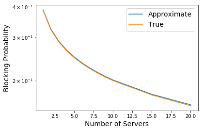
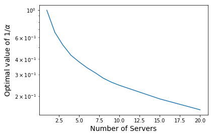
Given that the ESRT policy is more tractable than the DSRT policy, our first goal is to check if the performance of the former is a good approximation to the performance of the latter. The numerical analysis is done for the case when $\hat{D}=2$, and $\hat{T}=10$. i.e., the system is allowed to defer one or two customers. We then consider a sequence of queueing systems under the Halfin-Whitt scaling regime, with $\beta=0.1.$ In Figure 8(a), we compare the blocking probability under ESRT using the optimal computed value $\alpha^{*}(K)$ of the policy parameter, with the blocking probability under DSRT using $x=1/\alpha^{*}(K).$ Note that the two curves are nearly indistinguishable, suggesting that the approximation is sound (at least for small values of $\hat{D}$). In Figure 8(b), we plot $1/\alpha^{*}(K)$ v/s $K.$ Since $1/\alpha^{*}(K)$ decreases with $K,$ it follows that it is optimal to decrease the spacing between rearrivals as the size of the system grows under the Halfin-Whitt regime. This is to be expected, since the arrival rate and the service rate of the system grow nearly proportionately under this scaling regime.

(a) Approximate $P_{B}$

(b) Optimal $\frac{1}{\alpha}$ for ESRT

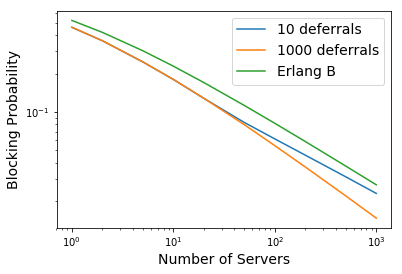
Next we study the impact of the maximum number of deferrals $\hat{D}.$ Under the Halfin-Whitt scaling regime as before, in Figure 9(a), we plot the optimal (with respect to the deferral parameter $\alpha$) blocking probability when $\hat{D}=10$ and $\hat{D}=1000,$ along with the Erlang B formula (which corresponds to $\hat{D}=0.$) For this case, we set $\hat{T}=1.$ Note that increasing the limit on the number of deferrals does improve the performance significantly. Moreover, it is well-known that the blocking probability of the Erlang B (M/M/$K$/$K$) system decays as $\Omega(1/\sqrt{K})$ under the Halfin-Whitt scaling (see [5]). The numerical results as shown in Figure 9(a), suggest that the decay of blocking probability of ESRT is also $\Omega(1/\sqrt{K})$ (note the nearly linear scaling of blocking probability with $K$ on a log-log scale), at least when $\hat{D}$ is small. Having a large value of $\hat{D}$ could possibly allow a $o(1/\sqrt{K})$ decay in the blocking probability. Formalizing this scaling behavior is an interesting avenue for future work.

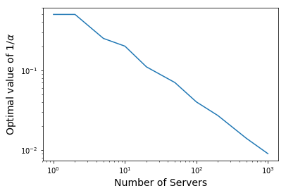
When $\hat{D}$ is 1000, we also plot the inverse of optimal deferral parameter $\alpha$ against the number of servers in Figure 9(b). Notice the nearly linear decay of $1/\alpha$ in the log-log plot, indicating a regularly varying scaling with the number of servers in the Halfin-Whitt regime. Characterizing the optimal deferral parameters for both ESRT and DSRT would also be illuminating.

(a) Performance Evaluation

(b) Optimal $\frac{1}{\alpha}$ for ESRT

V Concluding Remarks

Our work motivates several directions for future work including the following. One, characterizing the optimal parameter values and optimal blocking probabilities in a large system limit for DSRT/ESRT. Second, designing deferral policies operating under constraints on the number of deferrals and patience time that can beat the $1/\sqrt{K}$ blocking probability scaling under the Halfin-Whitt regime. Finding fundamental lower bounds on the blocking probability of such deferral policies would also be interesting.

References

- Artalejo and Gómez-Corral [1999] J. R. Artalejo and A. Gómez-Corral. Retrial queueing systems. Mathematical and Computer Modelling, 30(3-4):xiii–xv, 1999.
- Baccelli and Hebuterne [1981] F. Baccelli and G. Hebuterne. On queues with impatient customers. 1981.
- Doshi et al. [2015] B. Doshi, C. Kumar, P. Piyush, and M. Vutukuru. Webq: A virtual queue for improving user experience during web server overload. In 2015 IEEE 23rd International Symposium on Quality of Service (IWQoS), pages 135–140. IEEE, 2015.
- Halfin and Whitt [1981] S. Halfin and W. Whitt. Heavy-traffic limits for queues with many exponential servers. Operations research, 29(3):567–588, 1981.
- Jagerman [1974] D. L. Jagerman. Some properties of the erlang loss function. Bell System Technical Journal, 53(3):525–551, 1974.
- Kim and Kim [2016] J. Kim and B. Kim. A survey of retrial queueing systems. Annals of Operations Research, 247(1):3–36, 2016.
- Zeltyn and Mandelbaum [2005] S. Zeltyn and A. Mandelbaum. Call centers with impatient customers: many-server asymptotics of the m/m/n+ g queue. Queueing Systems, 51(3-4):361–402, 2005.