Robust cluster expansion of multicomponent systems using structured sparsity

Abstract

Identifying a suitable set of descriptors for modeling physical systems often utilizes either deep physical insights or statistical methods such as compressed sensing. In statistical learning, a class of methods known as structured sparsity regularization seeks to combine both physics- and statistics-based approaches. Used in bioinformatics to identify genes for the diagnosis of diseases, group lasso is a well-known example. Here in physics, we present group lasso as an efficient method for obtaining robust cluster expansions (CE) of multicomponent systems, a popular computational technique for modeling such systems and studying their thermodynamic properties. Via convex optimization, group lasso selects the most predictive set of atomic clusters as descriptors in accordance with the physical insight that if a cluster is selected, so should its subclusters. These selection rules avoid spuriously large fitting parameters by redistributing them among lower order terms, resulting in more physical, accurate, and robust CEs. We showcase these features of group lasso using the CE of bcc ternary alloy Mo-V-Nb. These results are timely given the growing interests in applying CE to increasingly complex systems, which demand a more reliable machine learning methodology to handle the larger parameter space.

I Introduction

Model building in physics requires both physical insights and statistics. In the cluster expansion (CE) of multicomponent systems (Sanchez et al., 1984), physical insights prescribe that the energies of atomic configurations obey a generalized Ising-like Hamiltonian. The energy $E\left(\sigma\right)$ of an atomic structure $\sigma$ can be expanded in terms of atomic clusters $\alpha$, where the cluster correlation functions $\Phi_{\alpha}\left(\sigma\right)$ serve as the basis set and the effective cluster interactions (ECIs) $V_{\alpha}$ as the coefficients:

$$E\left(\sigma\right) = \sum_{\alpha}\Phi_{\alpha}\left(\sigma\right)V_{\alpha}.$$ (1)

Statistically optimal values of the ECIs could be obtained via fitting to Eq. 1 the energies of a training set of structures, usually calculated from first principles. When appropriately truncated, the CE is an accurate model for efficiently predicting the energies (Blum and Zunger, 2004; Tan et al., 2012; Ng and Tan, 2013; Wróbel et al., 2015; Maisel et al., 2016) or associated properties (Ferreira et al., 1991; Van der Ven et al., 2001; Chan et al., 2010; Maisel et al., 2012; Wang et al., 2012; Fernández-Caballero et al., 2017) of different atomic configurations.

However, selecting the appropriate set of atomic clusters as descriptors is challenging: selections based on physical intuition are not robust, while those based on statistics are not physical. Initially, CE was largely applied to binary alloys (Connolly and Williams, 1983; Lu et al., 1991; Wolverton et al., 1992; Zunger, 1994; Garbulsky and Ceder, 1994; Fontaine, 1994; Lu et al., 1995; Garbulsky and Ceder, 1995; Wolverton and Zunger, 1995; Ozoliņš et al., 1998; Kohan et al., 1998; Müller and Zunger, 2001; Zunger et al., 2002; van de Walle and Asta, 2002; Blum and Zunger, 2004). Thereafter, it has been applied to more complex systems, including ternary to quinary alloys (Wróbel et al., 2015; Maisel et al., 2016; Ji and Jung, 2017; Feng et al., 2017; Nguyen et al., 2017; Fernández-Caballero et al., 2017), semiconductors (Ferreira et al., 1991; Burton et al., 2011), battery materials (Van der Ven and Ceder, 2004; Persson et al., 2010), clathrates (Ångqvist et al., 2016; Ångqvist and Erhart, 2017), magnetic alloys (Drautz and Fähnle, 2004, 2005; Lavrentiev et al., 2010), and nanoscale alloys (Wang et al., 2012; Tan et al., 2012; Kang et al., 2013; Ng and Tan, 2013; Cao and Mueller, 2015, 2016; Tan et al., 2017; Cao et al., 2018). In complex systems, the reduced symmetry increases the number of symmetrically distinct clusters, exacerbating the cluster selection problem. With growing enthusiasm in applying CE to higher component systems, such as high-entropy alloys (Fernández-Caballero et al., 2017), it is timely to introduce an improved machine-learning procedure for creating reliable CEs with physically meaningful and robust ECIs.

Currently, there are two prevalent approaches for cluster selection. The first emphasizes using physical insights, such as via specific priors in the Bayesian framework (Mueller and Ceder, 2009) or via selection rules to incorporate smaller clusters before larger ones (van de Walle and Ceder, 2002; Zarkevich and Johnson, 2004). The second approach espouses using sparsity-driven regularization such as compressed sensing (Hart et al., 2005; Drautz and Díaz-Ortiz, 2006; Nelson et al., 2013a, b; Maisel et al., 2016; Ångqvist et al., 2016; Ångqvist and Erhart, 2017). Fundamentally, CE is a standard linear regression problem $y=X\beta$—the response $y_{i}$ is the first-principles energy of the $i$th structure in the training set $\left\{\sigma\right\}$, the coefficient $\beta_{j}$ is the ECI of the $j$th cluster, and the component $x_{ij}$ of the design matrix $X$ is the correlation function $\Phi_{j}\left(\sigma_{i}\right)$ of structure $i$ with respect to cluster $j$. Typically, the optimal $\hat{\beta}$ is given by the regularized least-squares solution

$$\hat{\beta} = \operatorname*{argmin}_{\beta}\left\|y-X\beta\right\|_{2}^{2}+g\left(\beta\right),$$ (2)

where the $\ell_{p}$-norm is defined by $\left\|z\right\|_{p}=\left(\sum_{i}\left|z_{i}\right|^{p}\right)^{1/p}.$ The penalty function $g\left(\beta\right)$ constrains $\beta$ to reduce overfitting and is key to high prediction accuracy for structures outside the training set. In compressed sensing (Candes et al., 2006; Candes and Wakin, 2008), the least absolute shrinkage and selection operator (lasso) $g\left(\beta\right)\propto\left\|\beta\right\|_{1}$ selects atomic clusters by favoring parsimonious models (Nelson et al., 2013a, b); such models are more interpretable and simpler for quick computation, for example, in Monte-Carlo simulations.

In this paper, we present group lasso regularization (Yuan and Lin, 2006) as an efficient method for obtaining reliable CEs of multicomponent systems. As an example of structured sparsity in machine learning, group lasso combines sparsity-driven regularization with physical insights to select atomic clusters as descriptors. We show that even with the large parameter space of ternary alloys and beyond, the resulting truncated CE remains sparse and robust with interpretable ECIs. With a specially constructed convex penalty $g\left(\beta\right)$, group lasso imposes the physical insight that a cluster is selected only after all its subclusters. These selection rules avoid spuriously large fitting parameters by redistributing them among lower order terms, resulting in more physical, accurate, and robust CEs. We will demonstrate these features of group lasso via the CE of ternary bcc alloy Mo-V-Nb.

II Methods

II.1 Group lasso

Group lasso is an extension of the well-known lasso regularization (Tibshirani, 1996; Hastie et al., 2015). Using the nonanalyticity of the penalty functions, both methods favor sparse solutions to the linear regression problem $y=X\beta$. For example, the lasso penalty is $g\left(\beta\right)=\lambda\left\|\beta\right\|_{1}$ with hyperparameter $\lambda$, which has been studied in the context of compressed sensing CE (Nelson et al., 2013a, b). In this case, the sparsity of the regularized solution from Eq. 2 can be understood in the dual picture

$$\hat{\beta} = \operatorname*{argmin}_{\beta}\left\|y-X\beta\right\|_{2}^{2},\text{ with }\left\|\beta\right\|_{1}<\tau,$$ (3)

where $\tau$ is inversely related to $\lambda$. Fig. 1a illustrates the constraint $\left\|\beta\right\|_{1}<\tau$ for $\beta\in\mathbb{R}^{3}$. This constraint shrinks the least-squares solution to one that tends to lie on the corners/edges of the constraint highlighted in Fig. 1a. The resulting regularized solution is therefore sparse with some $\hat{\beta}_{i}$ vanishing.

(a)

(b)

Figure 1: The constraints on $\left\{\beta_{1},\beta_{2},\beta_{3}\right\}$ in (a) lasso and (b) group lasso regularizations. The corners/edges (in light blue) of these constraints correspond to sparse solutions. In (b), coefficients $\beta_{1}$ and $\beta_{2}$ are grouped, while $\beta_{3}$ remains a singleton. This grouping favors solutions with $\beta_{1},\beta_{2}$ either both zero or both nonzero.

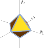
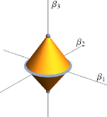
In conventional lasso, the sparse solution is determined from a statistical fit, with little room for incorporating pertinent physical insights. In contrast, group lasso seeks a more physically meaningful solution by ensuring that physically-related coefficients are either all zero or all nonzero together as a group. For example, when applied to gene expression data for the diagnosis of diseases in bioinformatics, group lasso ensures that genes with coordinated functions are either all excluded or all included in the model (Ma et al., 2007). For CE, we will use group lasso to impose physical cluster selection rules.

In group lasso, the coefficients $\beta$ are partitioned into $J$ groups $\theta_{1},\ldots,\theta_{J}$, where $\theta_{j}\in\mathbb{R}^{p_{j}}$ is a group of $p_{j}$ coefficients. Let $Z_{j}$ be the matrix formed by the columns of $X$ corresponding to the group $\theta_{j}$. Then, the regularized solution is

$$\hat{\beta} = \operatorname*{argmin}_{\beta}\frac{1}{2}\left\|y-\sum_{j=1}^{J}Z_{j}\theta_{j}\right\|_{2}^{2}+\lambda\sum_{j=1}^{J}\sqrt{p_{j}}\left\|\theta_{j}\right\|_{2},$$ (4)

with hyperparameter $\lambda$. Notice that unlike in the least-squares term, the $\ell_{2}$-norm in the penalty is not squared and is therefore nonanalytic. It is this nonanalyticity that imposes sparsity.

In the dual picture, the unregularized least-squares solution is now constrained by

$$\sum_{j=1}^{J}\sqrt{p_{j}}\left\|\theta_{j}\right\|_{2} < \tau.$$ (5)

Fig. 1b illustrates this group-lasso constraint for the case with three coefficients and the groups $\theta_{1}=\left(\beta_{1},\beta_{2}\right)$ and $\theta_{2}=\beta_{3}$. In this case, Eq. 4 simplifies to

$$\hat{\beta} = \operatorname*{argmin}_{\beta}\frac{1}{2}\left\|y-X\beta\right\|_{2}^{2}+\lambda\left(\sqrt{2}\sqrt{\beta_{1}^{2}+\beta_{2}^{2}}+\left|\beta_{3}\right|\right).$$ (6)

Compared to the lasso case in Fig. 1a, sharp corners/edges (representing sparse solutions) are now at $\beta_{1},\beta_{2}\neq 0,\beta_{3}=0$ and $\beta_{1}=\beta_{2}=0,\beta_{3}\neq 0$. Group lasso thus favors solutions with $\beta_{1},\beta_{2}$ either both zero or both nonzero. In general, coefficients in the same group $\theta_{j}$ are either all zero or all nonzero.

When each group in Eq. 4 is a singleton, that is $p_{j}=1$ for all $j$, the regularized solution reduces to that of lasso

$$\hat{\beta}_{\text{lasso}} = \operatorname*{argmin}_{\beta}\frac{1}{2}\left\|y-X\beta\right\|_{2}^{2}+\lambda\left\|\beta\right\|_{1}.$$ (7)

We will use this to benchmark the performance of group lasso. Since the penalty terms for both lasso and group lasso are convex, the regularized solutions can be efficiently obtained by convex optimization. Note that the weights $\sqrt{p_{j}}$ in the penalty term of Eq. 4 ensure that groups of different sizes are penalized equally. Without these weights, a group with many coefficients will unfairly dominate the penalty term. We next discuss the cluster selection rules we wish to impose using group lasso.

II.2 Hierarchical cluster selection rules

In CE, the energy of an atomic configuration is expanded in terms of the atomic clusters and their associated ECIs. In general, since a cluster $b$ is a higher order correction to its subcluster $a\subset b$, the ECI $\beta_{b}\neq 0$ only if the subcluster ECI $\beta_{a}\neq 0$. I.e., a CE should include a cluster only if all its subclusters are also included. This is the hierarchical cluster selection rule we adopt here. Similar rules have been used for the CEs of binary systems (van de Walle and Ceder, 2002; Zarkevich and Johnson, 2004; Sluiter and Kawazoe, 2005; Zarkevich et al., 2008; Mueller and Ceder, 2009; Tan et al., 2012; Ng and Tan, 2013; Tan et al., 2017). Here, we extend such rules to alloy systems with more components.

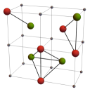
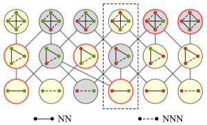
Without vacancies, an $m$-component system requires the tracking of $m-1$ independent atomic species. For $m\geq 3$, the key distinction from binaries is that for a given cluster, multiple decorations (of independent atomic species) need to be accounted for when considering subcluster relations. For a given independent decoration, the correlation function in Eq. 1 is defined as the number of clusters present in the atomic structure. For example, Fig. 2a shows three decorated clusters of a ternary system on a bcc lattice. The pair $a$, triplet $b$, and quadruplet $c$ are related by $a\subset b$, $a\subset c$ and $b\not\subset c$. These relations are represented graphically in Fig. 2b, where each bubble contains a cluster (shown as a 2D schematic) with lines connecting it to its subclusters with one fewer atom. The three clusters in Fig. 2a correspond to those in the dashed box in Fig. 2b. The set of highlighted clusters (bubbles with yellow background) is an example satisfying the hierarchical cluster selection rules, while the set with red borders does not. Our work aims to use group lasso to obtain cluster sets that obey the hierarchical rules.

(a)

(b)

Figure 2: Atomic clusters of a bcc ternary system, with atomic species distinguished by colors. (a) Examples of the smallest pair, triplet, and quadruplet. (b) A graphical representation of the subcluster relations. Each bubble contains a cluster shown as a 2D schematic, with lines connecting it to all its subclusters with one fewer atom. The clusters in the dashed box correspond to those in (a). The highlighted vertices form a set of clusters obeying the hierarchical selection rules, while those with a red border do not.

II.3 Cluster selection with group lasso

Imposing the cluster selection rules using group lasso is a subtle but important point. This is because the hierarchical rules require overlapping groups of ECIs, which are incompatible with how group lasso is formulated in Sec. II.1. The solution is to use a variant of group lasso known as overlap group lasso (Jacob et al., 2009).

To show how this variant of group lasso can impose the cluster selection rules, we consider just two clusters $c_{1}\subset c_{2}$ and the corresponding ECIs $\beta_{1}$ and $\beta_{2}$. To have $\beta_{2}\neq 0$ imply $\beta_{1}\neq 0$ (as per the selection rules), we first write $\beta_{1}=\theta_{11}+\theta_{21}$ and $\beta_{2}=\theta_{22}$. Then, grouping together $\theta_{21}$ and $\theta_{22}$, we apply group lasso using Eq. 4 to find the optimal $\theta_{11},\theta_{21}$, and $\theta_{22}$:

$$\hat{\theta} = \operatorname*{argmin}_{\theta}\frac{1}{2}\left\|y-x_{1}\left(\theta_{11}+\theta_{21}\right)-x_{2}\theta_{22}\right\|_{2}^{2}$$ (8)

$$+\lambda\left(\left|\theta_{11}\right|+\sqrt{2}\sqrt{\theta_{21}^{2}+\theta_{22}^{2}}\right).$$

As discussed, the form of group lasso’s penalty ensures that $\theta_{21}$ and $\theta_{22}$ are either both zero or both nonzero. Consequently, $\beta_{2}\neq 0$ implies that $\beta_{1}\neq 0$ (almost surely), but we can still have $\beta_{2}=0$ with $\beta_{1}\neq 0$. This is precisely the selection rule corresponding to the subcluster relation $c_{1}\subset c_{2}$.

For a general set of $p$ clusters $\left\{c_{1},\ldots,c_{p}\right\}$, group lasso can similarly impose the selection rules. First, we write the ECIs $\beta=\left(\beta_{1},\ldots,\beta_{p}\right)^{T}$ as a sum of $p$ groups of coefficients: $\beta=\sum_{j=1}^{p}\nu_{j}$ where $\nu_{j}\in\mathbb{R}^{p}$ is a vector constrained to be zero everywhere except in positions corresponding to $c_{j}$ and its subclusters. That is, we fix $v_{j,k}=0$ for all $k$ such that $c_{k}\not\subseteq c_{j}$. Then, the group lasso solution for the unconstrained components is analogous to Eq. 8:

$$\hat{\nu} = \operatorname*{argmin}_{\nu}\frac{1}{2}\left\|y-X\sum_{j=1}^{p}\nu_{j}\right\|_{2}^{2}+\lambda\sum_{j=1}^{p}\sqrt{p_{j}}\left\|\nu_{j}\right\|_{2},$$ (9)

where $p_{j}$ is the number of subclusters of $c_{j}$ (including $c_{j}$ itself). That is, $p_{j}$ is the number of unconstrained components in $\nu_{j}$.

Here, we verify that Eq. 9 works as intended: the selection of a cluster $c_{j}$ should imply the selection of its subcluster $c_{l}\subset c_{j}$. Given $\beta_{j}\neq 0$, we have $\nu_{k,j}\neq 0$ for some $k$ such that $c_{j}\subseteq c_{k}$. Then, for a subcluster $c_{l}\subset c_{j}$ (and hence $c_{l}\subset c_{k}$), the $\left\|v_{k}\right\|_{2}$ term in the penalty ensures that $\nu_{k,l}\neq 0$. Consequently, $\beta_{l}\neq 0$, as required.

III Results

We showcase the features of group lasso via the CE of bcc ternary alloy Mo-V-Nb, whose constituent elements are well-known refractory metals. Previously, CE has been used to study the ground states of binary alloys V-Nb (Ravi et al., 2012) and Mo-Nb (Blum and Zunger, 2005; Huhn and Widom, 2013). Here, we benchmark the performance of group lasso (Eq. 9) against lasso (Eq. 7). The former method imposes the hierarchical cluster selection rules, while the latter performs regularization based just on statistics. The value of the hyperparameter $\lambda$ in each method is fixed by cross-validation (CV). Our training structures have small unit cells with up to six atoms. We use 239 clusters consisting of pairs, triplets, …, and six-body clusters, with 1654 cluster selection rules. As we will see, group lasso tends to produce CEs that are more physical, accurate, and robust than those from lasso. The appendix contains further technical details about our implementation.

Physicalness:

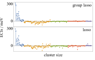
Fig. 3 shows the values of the ECIs based on $800$ training structures. The group lasso ECIs, by construction, obey all the cluster selection rules, and they satisfy the physical intuition that ECIs generally weaken with increasing cluster size. This behavior suggests that the CE is converging, given our initial pool of clusters. In contrast, the lasso ECIs obey only $\sim 87\%$ of the rules, and numerous large clusters have abnormally large ECIs. Therefore, via the selection rules, group lasso redistributes these spurious spikes in lasso among lower-order terms. While this redistribution decreases sparsity (205 nonzero ECIs for group lasso vs 180 for lasso), CEs from group lasso have more physical trends in the ECIs than from lasso. These general behaviors are observed regardless of the training set choices.

Figure 3: The values of $239$ ECIs based on $800$ training structures. Pairs, triplets, quadruplets, 5-bodies, and 6-bodies are colored blue, orange, green, red, and purple, respectively. The ECIs from group lasso are well-behaved—larger clusters generally have smaller ECIs—while for lasso, several isolated spikes corresponding to large ECIs are observed among the higher-order clusters (quadruplets and beyond).

Accuracy:

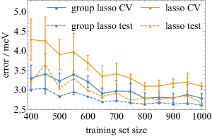
In addition to the training structures, we also have $500$ test structures with large $16$-atom unit cells not used for training. For both lasso and group lasso, Fig. 4 shows the CV scores and test errors decreasing as the number of training structures increases, signifying the convergence of the CEs. For either method, the CV scores and test errors are comparable. These observations imply that the lasso class of methods are able to distill the essential physics from training with just small structures, reliably predicting the energies of larger structures not in the training set. This is advantageous for ternary alloys and beyond, because of the huge number of large structures in these systems. For all training set sizes, group lasso is consistently more accurate than lasso (smaller CV scores and test errors). Therefore, the incorporation of physical hierarchy improves not only the physical interpretability of the ECIs but also the predictive capability of the CE. Group lasso reduces overfitting by redistributing the contributions from unphysical spikes in lasso’s ECIs among numerous smaller clusters that are more important.

Figure 4: Five-fold cross-validation (CV) scores and test errors for group lasso and lasso versus training set size. The errors of group lasso are consistently lower than lasso’s. The error bars for the CV scores correspond to one standard deviation among the five folds.

Robustness:

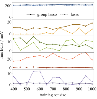
The ECIs of a robust CE should converge towards the true physical values when more training structures are used. As such, a lack of robustness is signified by ECIs wildly fluctuating with respect to the size of the training set. The degree of fluctuations can be concisely illustrated using the root-mean-square (rms) of the ECIs in each cluster category (pairs, triplets, $\ldots$, and six-bodies). Fig. 5 shows that the five rms ECIs from group lasso are largely stable with respect to the number of training structures. However, the ECIs from lasso tend to vary wildly for the higher order clusters. This distinction shows that group lasso produces CEs that are more robust; the ECIs are more physically interpretable for group lasso (especially for higher order clusters), as they tend to fluctuate less with different training sets.

Figure 5: The root-mean-square ECIs with respect to the number of training structures for different category of clusters, namely, from top to bottom, pairs, triplets, quadruplets, 5-bodies, and 6-bodies. For higher order clusters, the ECIs of group lasso tend to fluctuate much less than those of lasso.

IV Discussions and conclusion

As mentioned in Sec. II.2, similar hierarchical cluster selection rules have been used for CE (van de Walle and Ceder, 2002; Zarkevich and Johnson, 2004; Sluiter and Kawazoe, 2005; Zarkevich et al., 2008; Mueller and Ceder, 2009; Tan et al., 2012; Ng and Tan, 2013; Tan et al., 2017). Compared to previous works, the combination of these rules with sparsity-driven regularization in our work leads to more robust ECIs. This is because regularization shrinks the values of the selected ECIs to avoid spuriously large terms. Furthermore, since previous methods involve evaluating different combinations of clusters separately to find the optimal one, these methods become less computationally feasible for ternary systems and beyond, where many more combinations of clusters need to be explored. This is so unless the search space is shrunk by imposing additional selection criteria, for example, if an $n$-body cluster is included, then all $n$-body clusters of smaller spatial extent are also included (van de Walle and Ceder, 2002; Zarkevich and Johnson, 2004). We do not impose these additional criteria in our work; they might be too restrictive for ternaries and beyond because, for example, the inclusion of A-B pairs up to a certain spatial extent should not impact the spatial extent of pairs for other decorations (i.e., B-C, A-C).

In Ref. (Sluiter and Kawazoe, 2005), the authors studied the invariance of CE under linear transformations of the site occupation variables. The authors showed that invariance is preserved only when the hierarchical cluster selection rules are obeyed. We emphasize that our group lasso implementation obeys the hierarchical rules, whereas standard lasso does not. Hence, our work presents a way for preserving the invariance of CE.

In conclusion, we presented group lasso (Yuan and Lin, 2006) as an efficient method for producing reliable CEs of multicomponent alloys, resulting in accurate and robust surrogate models for predicting thermodynamic properties. A type of structured sparsity regularization, group lasso combines statistical learning with physical insights to select atomic clusters as descriptors for the CE model. Via convex optimization, group lasso imposes the cluster selection rules that a cluster is selected only after all its subclusters. These rules avoid spuriously large fitting parameters by redistributing them among numerous lower order terms, resulting in more physical, accurate, and robust CEs. These results are timely given the growing interests in applying CE to increasingly complex systems, where the larger parameter space demands a more reliable machine learning methodology to construct robust models. Furthermore, this work should inspire applying structured sparsity in modeling other physical systems.

*

Appendix

In this appendix, we present the technical details about our implementation of cluster expansion (CE) and group lasso.

.1 First-principles calculations

The energies of the training and test structures are calculated based on density functional theory (DFT) with the Vienna Ab initio Simulation Package (VASP) (Kresse and Furthmüller, 1996a, b). We use the Perdew, Burke, and Ernzerhof exchange correlation based on the generalized gradient approximation (Perdew et al., 1996, 1997). The PAW potentials are used with the outer $p$ semi-core states included in the valence states (Blöchl, 1994; Kresse and Joubert, 1999). Plane-wave cutoffs are set to 520 eV and all atomic coordinates (including lattice vectors) were fully relaxed until the calculated Hellmann-Feynman force on each atom was less than $0.015\mbox{ eV}/\text{\AA}$. Calculations are non spin-polarized as Mo, Nb, and V are not known to be strongly magnetic. The $k$-point mesh is generated using a Gamma grid and density of $200\ \text{\AA}^{-3}$.

.2 Normalization choice for cluster correlations

The general expression for CE given by

$$E\left(\sigma\right) = \sum_{\alpha}\Phi_{\alpha}\left(\sigma\right)V_{\alpha}.$$ (10)

can be rewritten to account for the degeneracy of the clusters in a specific lattice (Zarkevich et al., 2007). For any rescaling factor $\eta_{\alpha}>0$, Eq. 10 is invariant under the transformation $\Phi_{\alpha}\left(\sigma\right)\rightarrow\Phi_{\alpha}\left(\sigma\right)\eta_{\alpha}$ and $V_{\alpha}\rightarrow V_{\alpha}/\eta_{\alpha}$. The choice of $\eta_{\alpha}$ depends on whether degeneracy factors are subsumed into $\Phi_{\alpha}\left(\sigma\right)$ or $V_{\alpha}$. Here, we choose $\eta_{\alpha}$ such that $\Phi_{\alpha}=N_{\alpha}/\widetilde{N}_{\alpha}$, where $N_{\alpha}\left(\widetilde{N}_{\alpha}\right)$ is the number of clusters in the structure that are symmetrically equivalent to cluster $\alpha$, (without) taking into account the decorations. This normalization gives $0\leq\Phi_{\alpha}\leq 1$ for all $\alpha$’s, which is convenient because the convergence of $V_{\alpha}$ with respect to cluster size would directly reflect the convergence of the CE.

In practice, we use occupation variables $\xi$ to describe the atomic species at each lattice site of a structure: $\xi_{A}\left(\sigma_{j}\right)$ equals 1 (0) if site $j$ in structure $\sigma$ is (not) occupied by species $A\in\left\{\text{Mo},\text{V},\text{Nb}\right\}$. Note that this is distinct from the orthogonal basis in an alternate CE formalism (Sanchez et al., 1984). Then, the correlation function of structure $\sigma$ with respect to cluster $\alpha$ is computed using

$$\Phi_{\alpha}\left(\sigma\right) = \frac{1}{\widetilde{N}_{\alpha}}\sum_{c}\prod_{j\in c}\xi_{c_{j}}\left(\sigma_{j}\right),$$ (11)

where the sum is over all clusters $c$ symmetrically equivalent to $\alpha$. The product is over all sites $j$ in the cluster, with $c_{j}$ giving the atomic species at site $j$. We reiterate that for ternary alloys and beyond, decorations need to be taken into account when considering symmetrically equivalent clusters.

.3 Formation energy

In general, either the configuration energy $E\left(\sigma\right)$ or the formation energy $E_{F}\left(\sigma\right)$ could be used to train the CE. In this work, we use the latter, which is defined as

$$E_{F}\left(\sigma\right) = E\left(\sigma\right)-\sum_{A}\rho_{A}\left(\sigma\right)E\left(\sigma_{A}^{\text{pure}}\right),$$ (12)

where $\rho_{A}\left(\sigma\right)$ is the concentration of species $A$ in the structure $\sigma$, and $\sigma_{A}^{\text{pure}}$ is the pure system of species $A$. With the CE of $E\left(\sigma\right)$ from Eq. 10, the formation energy can be expanded in terms of the ECIs:

$$E_{F}\left(\sigma\right) = \sum_{\alpha}\left[\Phi_{\alpha}\left(\sigma\right)-\sum_{A}\rho_{A}\left(\sigma\right)\Phi_{\alpha}\left(\sigma_{A}^{\text{pure}}\right)\right]V_{\alpha}.$$ (13)

Because the expression in the square bracket vanishes exactly for the empty cluster and singlets, the formation energy is expandable in terms of just pairs and larger clusters (Zarkevich et al., 2008). This form of the formation energy also naturally gives $E_{F}=0$ for pure systems. Then, writing Eq. 13 as the linear regression problem $y=X\beta$, we standardize the columns of $X$ to have unit $\ell_{2}$-norm before applying group lasso (or lasso), as per common practice (Hastie et al., 2015). That is, denoting the $i$th column of $X$ by $x_{i}$, we apply the invariant rescaling $x_{i}\rightarrow x_{i}/\left\|x_{i}\right\|_{2}$ and $\beta_{i}\rightarrow\beta_{i}\left\|x_{i}\right\|_{2}$ such that $\left\|x_{i}\right\|_{2}=1$ for all $i$’s.

Figure 6: The DFT formation energies $E_{F}$ of $1081$ derivative structures with up to 6-atom unit cell in a bcc lattice, with respect to compositions. Structures with $E_{F}>0$ are not shown. Redder (bluer) points are structures with smaller (larger) unit cells. The blue translucent surface is the ground state hull, with ground state structures represented by larger points. The ternary plot shows the compositions of the structures, with ground state structures highlighted in white.

.4 Generation of training and test structures

Ideally, the structures in a training set should be sufficiently varied to capture all important physics of the system. To cover a wide range of the configurational space, training structures can be selected either randomly (Nelson et al., 2013a, b) or systematically to maximize the covariance matrix of the correlation functions (Seko et al., 2009).

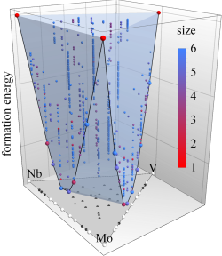
In practice, computational constraints limit the number of DFT calculations and favor training structures with smaller unit cells. This limitation is especially severe for ternary alloys and beyond, because the configurational space grows combinatorially with the number of atomic species. Therefore, we select our training structures from a pool of 1081 derivative structures, systematically generated up to 6-atom unit cell (Hart and Forcade, 2008; Hart et al., 2012). Fig. 6 shows the DFT formation energies and compositions of these structures. Notably, lower energy structures tend to have smaller unit cells. Following the smallest-first algorithm (Ferreira et al., 1991), structures with smaller unit cells are chosen first. We exclude the three pure systems because their formation energies given by Eq. 13 are identically zero.

To verify that such training sets suffice for ternary systems, we test the CE trained using small structures against a test set (holdout set) of larger structures. The test set consists of 500 randomly selected 16-atom derivative structures; this set is not used to train our CE model, but it serves to determine the testing/prediction error. The ternary plot in Fig. 7 shows the compositions of these test structures compared to those of the training set.

Figure 7: A ternary plot showing the compositions of the 1081 training structures and 500 test structures.

.5 Initial set of clusters

In our CE model, we treat V and Nb as the independent species, while Mo is treated as dependent. As such, only clusters formed by Mo and V atoms are required. In the bcc lattice, we consider up to the 9th-nearest-neighbor (9NN) pairs, triplets with a 5NN cutoff, and four-body to six-body clusters with a 3NN cutoff. These correspond to an initial pool of 239 symmetrically distinct clusters, consisting of 27 pairs, 84 triplets, 54 four-body clusters, 56 five-body clusters, and 18 six-body clusters. Among these clusters are 1654 subcluster relations, which group lasso uses to derive the final truncated CE based on the cluster selection rules.

Figure 8: Top: The five-fold cross validation (CV) score of group lasso with respect to the hyperparameter $\lambda$, using $800$ training structures. The green vertical line denotes the minimum CV score. The red vertical line is one-standard error away from the minimum and gives the optimal $\lambda$. Inset: a closeup of the same plot. Bottom: The six ECIs of the nearest-neighbor (blue) and next-nearest-neighbor (yellow) pairs with respect to $\lambda$.

.6 Tuning of hyperparameter $\lambda$

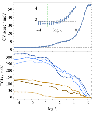
Using the DFT formation energies of the training structures, we use group lasso to select a properly truncated CE set from the initial 239 distinct clusters. The group lasso minimization problem is efficiently solved using a block coordinate descent algorithm (Hastie et al., 2015), which reduces the multidimensional minimization problem to a sequence of root-finding problems in 1D. Overfitting (underfitting) happens when the hyperparameter $\lambda$ is too small (large). The optimal $\lambda$ is selected based on a five-fold cross validation (CV) with the one-standard error rule (Hastie et al., 2015), as illustrated in Fig. 8 (top). I.e., the optimal $\lambda$ corresponds to the most regularized model with CV score within one standard error of the minimal CV score. The bottom plot of Fig. 8 shows coefficient shrinkage and cluster selection in group lasso. As $\lambda$ decreases, the model becomes less regularized and the ECIs generally increase; the solution is also less sparse as more ECIs become nonzero.

References

- Sanchez et al. (1984) J. Sanchez, F. Ducastelle, and D. Gratias, Physica A: Statistical Mechanics and its Applications 128, 334 (1984).
- Blum and Zunger (2004) V. Blum and A. Zunger, Physical Review B 69 (2004), 10.1103/PhysRevB.69.020103.
- Tan et al. (2012) T. L. Tan, L.-L. Wang, D. D. Johnson, and K. Bai, Nano Letters 12, 4875 (2012).
- Ng and Tan (2013) M.-F. Ng and T. L. Tan, Nano Letters 13, 4951 (2013).
- Wróbel et al. (2015) J. S. Wróbel, D. Nguyen-Manh, M. Y. Lavrentiev, M. Muzyk, and S. L. Dudarev, Physical Review B 91 (2015), 10.1103/PhysRevB.91.024108.
- Maisel et al. (2016) S. B. Maisel, M. Höfler, and S. Müller, Physical Review B 94 (2016), 10.1103/PhysRevB.94.014116.
- Ferreira et al. (1991) L. Ferreira, S.-H. Wei, and A. Zunger, The International Journal of Supercomputing Applications 5, 34 (1991).
- Van der Ven et al. (2001) A. Van der Ven, G. Ceder, M. Asta, and P. D. Tepesch, Physical Review B 64, 184307 (2001).
- Chan et al. (2010) M. K. Y. Chan, J. Reed, D. Donadio, T. Mueller, Y. S. Meng, G. Galli, and G. Ceder, Physical Review B 81, 174303 (2010).
- Maisel et al. (2012) S. B. Maisel, M. Höfler, and S. Müller, Nature 491, 740 (2012).
- Wang et al. (2012) L.-L. Wang, T. L. Tan, and D. D. Johnson, Physical Review B 86 (2012), 10.1103/PhysRevB.86.035438.
- Fernández-Caballero et al. (2017) A. Fernández-Caballero, J. S. Wróbel, P. M. Mummery, and D. Nguyen-Manh, Journal of Phase Equilibria and Diffusion 38, 391 (2017).
- Connolly and Williams (1983) J. W. D. Connolly and A. R. Williams, Physical Review B 27, 5169 (1983).
- Lu et al. (1991) Z. W. Lu, S.-H. Wei, and A. Zunger, Physical Review Letters 66, 1753 (1991).
- Wolverton et al. (1992) C. Wolverton, G. Ceder, D. de Fontaine, and H. Dreysse, Physical Review B 45, 13105 (1992).
- Zunger (1994) A. Zunger, in Statics and Dynamics of Alloy Phase Transformations, Vol. 319, edited by P. E. A. Turchi and A. Gonis (Springer US, Boston, MA, 1994) pp. 361–419.
- Garbulsky and Ceder (1994) G. D. Garbulsky and G. Ceder, Physical Review B 49, 6327 (1994).
- Fontaine (1994) D. D. Fontaine, in Solid State Physics, Vol. 47 (Elsevier, 1994) pp. 33–176.
- Lu et al. (1995) Z. W. Lu, B. M. Klein, and A. Zunger, Superlattices and Microstructures 18, 161 (1995).
- Garbulsky and Ceder (1995) G. D. Garbulsky and G. Ceder, Physical Review B 51, 67 (1995).
- Wolverton and Zunger (1995) C. Wolverton and A. Zunger, Physical Review B 52, 8813 (1995).
- Ozoliņš et al. (1998) V. Ozoliņš, C. Wolverton, and A. Zunger, Physical Review B 57, 6427 (1998).
- Kohan et al. (1998) A. F. Kohan, P. D. Tepesch, G. Ceder, and C. Wolverton, Computational Materials Science 9, 389 (1998).
- Müller and Zunger (2001) S. Müller and A. Zunger, Physical Review Letters 87, 165502 (2001).
- Zunger et al. (2002) A. Zunger, L. G. Wang, G. L. W. Hart, and M. Sanati, Modelling and Simulation in Materials Science and Engineering 10, 685 (2002).
- van de Walle and Asta (2002) A. van de Walle and M. Asta, Metallurgical and Materials Transactions A 33, 735 (2002).
- Ji and Jung (2017) H. Ji and Y. Jung, The Journal of Chemical Physics 146, 064103 (2017).
- Feng et al. (2017) R. Feng, P. K. Liaw, M. C. Gao, and M. Widom, npj Computational Materials 3 (2017), 10.1038/s41524-017-0049-4.
- Nguyen et al. (2017) M. C. Nguyen, L. Zhou, W. Tang, M. J. Kramer, I. E. Anderson, C.-Z. Wang, and K.-M. Ho, Physical Review Applied 8 (2017), 10.1103/PhysRevApplied.8.054016.
- Burton et al. (2011) B. P. Burton, S. Demers, and A. van de Walle, Journal of Applied Physics 110, 023507 (2011).
- Van der Ven and Ceder (2004) A. Van der Ven and G. Ceder, Electrochemistry Communications 6, 1045 (2004).
- Persson et al. (2010) K. Persson, Y. Hinuma, Y. S. Meng, A. Van der Ven, and G. Ceder, Physical Review B 82, 125416 (2010).
- Ångqvist et al. (2016) M. Ångqvist, D. O. Lindroth, and P. Erhart, Chemistry of Materials 28, 6877 (2016).
- Ångqvist and Erhart (2017) M. Ångqvist and P. Erhart, Chemistry of Materials 29, 7554 (2017).
- Drautz and Fähnle (2004) R. Drautz and M. Fähnle, Physical Review B 69, 104404 (2004).
- Drautz and Fähnle (2005) R. Drautz and M. Fähnle, Physical Review B 72, 212405 (2005).
- Lavrentiev et al. (2010) M. Y. Lavrentiev, D. Nguyen-Manh, and S. L. Dudarev, Physical Review B 81, 184202 (2010).
- Kang et al. (2013) J. Kang, S. Tongay, J. Li, and J. Wu, Journal of Applied Physics 113, 143703 (2013).
- Cao and Mueller (2015) L. Cao and T. Mueller, The Journal of Physical Chemistry C 119, 17735 (2015).
- Cao and Mueller (2016) L. Cao and T. Mueller, Nano Letters 16, 7748 (2016).
- Tan et al. (2017) T. L. Tan, H. M. Jin, M. B. Sullivan, B. Anasori, and Y. Gogotsi, ACS Nano 11, 4407 (2017).
- Cao et al. (2018) L. Cao, C. Li, and T. Mueller, Journal of Chemical Information and Modeling 58, 2401 (2018).
- Mueller and Ceder (2009) T. Mueller and G. Ceder, Physical Review B 80 (2009), 10.1103/PhysRevB.80.024103.
- van de Walle and Ceder (2002) A. van de Walle and G. Ceder, Journal of Phase Equilibria 23, 348 (2002).
- Zarkevich and Johnson (2004) N. A. Zarkevich and D. D. Johnson, Physical Review Letters 92 (2004), 10.1103/PhysRevLett.92.255702.
- Hart et al. (2005) G. L. W. Hart, V. Blum, M. J. Walorski, and A. Zunger, Nature Materials 4, 391 (2005).
- Drautz and Díaz-Ortiz (2006) R. Drautz and A. Díaz-Ortiz, Physical Review B 73, 224207 (2006).
- Nelson et al. (2013a) L. J. Nelson, G. L. W. Hart, F. Zhou, and V. Ozoliņš, Physical Review B 87 (2013a), 10.1103/PhysRevB.87.035125.
- Nelson et al. (2013b) L. J. Nelson, V. Ozoliņš, C. S. Reese, F. Zhou, and G. L. W. Hart, Physical Review B 88 (2013b), 10.1103/PhysRevB.88.155105.
- Candes et al. (2006) E. J. Candes, J. Romberg, and T. Tao, IEEE Transactions on Information Theory 52, 489 (2006).
- Candes and Wakin (2008) E. J. Candes and M. B. Wakin, IEEE Signal Processing Magazine 25, 21 (2008).
- Yuan and Lin (2006) M. Yuan and Y. Lin, Journal of the Royal Statistical Society: Series B (Statistical Methodology) 68, 49 (2006).
- Tibshirani (1996) R. Tibshirani, Journal of the Royal Statistical Society. Series B (Methodological) 58, 267 (1996).
- Hastie et al. (2015) T. Hastie, R. Tibshirani, and M. Wainwright, Statistical Learning with Sparsity: The Lasso and Generalizations, Chapman & Hall/CRC Monographs on Statistics & Applied Probability (CRC Press, 2015).
- Ma et al. (2007) S. Ma, X. Song, and J. Huang, BMC Bioinformatics 8, 60 (2007).
- Sluiter and Kawazoe (2005) M. H. F. Sluiter and Y. Kawazoe, Physical Review B 71, 212201 (2005).
- Zarkevich et al. (2008) N. A. Zarkevich, T. L. Tan, L.-L. Wang, and D. D. Johnson, Physical Review B 77 (2008), 10.1103/PhysRevB.77.144208.
- Jacob et al. (2009) L. Jacob, G. Obozinski, and J.-P. Vert, in Proceedings of the 26th Annual International Conference on Machine Learning, ICML ’09 (ACM, New York, NY, USA, 2009) pp. 433–440.
- Ravi et al. (2012) C. Ravi, B. K. Panigrahi, M. C. Valsakumar, and A. van de Walle, Physical Review B 85, 054202 (2012).
- Blum and Zunger (2005) V. Blum and A. Zunger, Physical Review B 72, 020104 (2005).
- Huhn and Widom (2013) W. P. Huhn and M. Widom, JOM 65, 1772 (2013).
- Kresse and Furthmüller (1996a) G. Kresse and J. Furthmüller, Computational Materials Science 6, 15 (1996a).
- Kresse and Furthmüller (1996b) G. Kresse and J. Furthmüller, Physical Review B 54, 11169 (1996b).
- Perdew et al. (1996) J. P. Perdew, K. Burke, and M. Ernzerhof, Physical Review Letters 77, 3865 (1996).
- Perdew et al. (1997) J. P. Perdew, K. Burke, and M. Ernzerhof, Physical Review Letters 78, 1396 (1997).
- Blöchl (1994) P. E. Blöchl, Physical Review B 50, 17953 (1994).
- Kresse and Joubert (1999) G. Kresse and D. Joubert, Physical Review B 59, 1758 (1999).
- Zarkevich et al. (2007) N. A. Zarkevich, T. L. Tan, and D. D. Johnson, Physical Review B 75, 104203 (2007).
- Seko et al. (2009) A. Seko, Y. Koyama, and I. Tanaka, Physical Review B 80 (2009), 10.1103/PhysRevB.80.165122.
- Hart and Forcade (2008) G. L. W. Hart and R. W. Forcade, Physical Review B 77 (2008), 10.1103/PhysRevB.77.224115.
- Hart et al. (2012) G. L. Hart, L. J. Nelson, and R. W. Forcade, Computational Materials Science 59, 101 (2012).