Generating Human Action Videos by Coupling 3D Game Engines and Probabilistic Graphical Models

Abstract

Deep video action recognition models have been highly successful in recent years but require large quantities of manually annotated data, which are expensive and laborious to obtain. In this work, we investigate the generation of synthetic training data for video action recognition, as synthetic data have been successfully used to supervise models for a variety of other computer vision tasks. We propose an interpretable parametric generative model of human action videos that relies on procedural generation, physics models and other components of modern game engines. With this model we generate a diverse, realistic, and physically plausible dataset of human action videos, called PHAV for “Procedural Human Action Videos”. PHAV contains a total of $39,982$ videos, with more than $1,000$ examples for each of $35$ action categories. Our video generation approach is not limited to existing motion capture sequences: $14$ of these $35$ categories are procedurally defined synthetic actions. In addition, each video is represented with $6$ different data modalities, including RGB, optical flow and pixel-level semantic labels. These modalities are generated almost simultaneously using the Multiple Render Targets feature of modern GPUs. In order to leverage PHAV, we introduce a deep multi-task (i.e. that considers action classes from multiple datasets) representation learning architecture that is able to simultaneously learn from synthetic and real video datasets, even when their action categories differ. Our experiments on the UCF-101 and HMDB-51 benchmarks suggest that combining our large set of synthetic videos with small real-world datasets can boost recognition performance. Our approach also significantly outperforms video representations produced by fine-tuning state-of-the-art unsupervised generative models of videos.

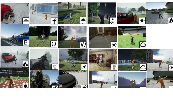
Figure 1: Procedurally generated human action videos. Depicted actions include: car hit, walking, kick ball, walking hug. Some are based on variations of existent MoCap sequences for these actions, whereas others have been programatically defined, with the final movement sequences being created on-the-fly through ragdoll physics and simulating the effect of physical interactions. For more example frames and an explanation of the legend icons seen here, cf. Appendix A.

1 Introduction

Successful models of human behavior in videos incorporate accurate representations of appearance and motion. These representations involve either carefully handcrafting features using prior knowledge, e.g., the dense trajectories of Wang et al. (2013), or training high-capacity deep networks with a large amount of labeled data, e.g., the two-stream network of Simonyan and Zisserman (2014). These two complementary families of approaches have often been combined to achieve state-of-the-art action recognition performance (Wang et al., 2015; De Souza et al., 2016). However, in this work we adopt the second family of approaches, which has recently proven highly successful for action recognition (Wang et al., 2016b; Carreira and Zisserman, 2017). This success is due in no small part to large labeled training sets with crowd-sourced manual annotations, e.g., Kinetics (Carreira and Zisserman, 2017) and AVA (Gu et al., 2018). However, manual labeling is costly, time-consuming, error-prone, raises privacy concerns, and requires massive human intervention for every new task. This is often impractical, especially for videos, or even unfeasible for pixel-wise ground truth modalities like optical flow or depth.

Using synthetic data generated from virtual worlds alleviates these issues. Thanks to modern modeling, rendering, and simulation software, virtual worlds allow for the efficient generation of vast amounts of controlled and algorithmically labeled data, including for modalities that cannot be labeled by a human. This approach has recently shown great promise for deep learning across a breadth of computer vision problems, including optical flow (Mayer et al., 2016), depth estimation (Lin et al., 2014), object detection (Vazquez et al., 2014; Peng et al., 2015), pose and viewpoint estimation (Shotton et al., 2011; Su et al., 2015a), tracking (Gaidon et al., 2016), and semantic segmentation (Ros et al., 2016; Richter et al., 2016).

In this work, we investigate procedural generation of synthetic human action videos from virtual worlds in order to generate training data for human behavior modeling. In particular, we focus on action recognition models. Procedural generation of such data is an open problem with formidable technical challenges, as it requires a full generative model of videos with realistic appearance and motion statistics conditioned on specific action categories. Our experiments suggest that our procedurally generated action videos can complement scarce real-world data.

Our first contribution is a parametric generative model of human action videos relying on physics, scene composition rules, and procedural animation techniques like “ragdoll physics” that provide a much stronger prior than just considering videos as tensors or sequences of frames. We show how to procedurally generate physically plausible variations of different types of action categories obtained by MoCap datasets, animation blending, physics-based navigation, or entirely from scratch using programmatically defined behaviors. We use naturalistic actor-centric randomized camera paths to film the generated actions with care for physical interactions of the camera. Furthermore, our manually designed generative model has interpretable parameters that allow to either randomly sample or precisely control discrete and continuous scene (weather, lighting, environment, time of day, etc), actor, and action variations to generate large amounts of diverse, physically plausible, and realistic human action videos.

Our second contribution is a quantitative experimental validation using a modern and accessible game engine (Unity®Pro) to synthesize a dataset of $39,982$ videos, corresponding to more than $1,000$ examples for each of $35$ action categories: $21$ grounded in MoCap data, and $14$ entirely synthetic ones defined procedurally. In addition to action labels, this dataset contains pixel-level and per-frame ground-truth modalities, including optical flow and semantic segmentation. All pixel-level data were generated efficiently using Multiple Render Targets (MRT). Our dataset, called PHAV for “Procedural Human Action Videos” (cf. Figure 1 for example frames), is publicly available for download. Our procedural generative model took approximately $2$ months of $2$ engineers to be programmed and our PHAV dataset $3$ days to be generated using $4$ gaming GPUs.

We investigate the use of this data in conjunction with the standard UCF-101 (Soomro et al., 2012) and HMDB-51 (Kuehne et al., 2011) action recognition benchmarks. To allow for generic use, and as predefined procedural action categories may differ from unknown a priori real-world target ones, we propose a multi-task (i.e. that considers action classes from multiple datasets) learning architecture based on the Temporal Segment Network (TSN) of  Wang et al. (2016b). We call our model Cool-TSN (cf. Figure 18) in reference to the “cool world” of Vázquez et al. (2011), as we mix both synthetic and real samples at the mini-batch level during training. Our experiments show that the generation of our synthetic human action videos can significantly improve action recognition accuracy, especially with small real-world training sets, in spite of differences in appearance, motion, and action categories. Moreover, we outperform other state-of-the-art generative video models (Vondrick et al., 2016) when combined with the same number of real-world training examples.

This paper extends (De Souza et al., 2017) in two main ways. First, we significantly expand our discussion of the generative model we use to control our virtual world and the generation of synthetic human action videos. Second, we describe our use of MRT for generating multiple ground-truths efficiently, rather than simply rendering RGB frames. In addition, we describe in detail the additional modalities we generate, with special attention to semantic segmentation and optical flow.

The rest of the paper is organized as follows. Section 2 presents a brief review of related work. In Section 3, we present our controllable virtual world and relevant procedural generation techniques we use within it. In Section 4 we present our probabilistic generative model used to control our virtual world. In Section 5 we show how we use our model to instantiate PHAV. In Section 6 we present our Cool-TSN deep learning algorithm for action recognition, reporting our quantitative experiments in Section 7. We then discuss possible implications of this research and offer prospects for future work in Section 8, before finally drawing our conclusions in Section 9.

2 Related work

Most works on action recognition rely exclusively on reality-based datasets. In this work, we compare to UCF-101 and HMDB-51, two standard action recognition benchmarks that are widely used in the literature. These datasets differ not only in the number of action categories and videos they contain (cf. Table 1), but also in the average length of their clips and their resolution (cf. Table 2), and in the different data modalities and ground-truth annotations they provide. Their main characteristics are listed below:

• UCF-101 (Soomro et al., 2012) contains 13,320 video clips distributed over 101 distinct classes. This is the dataset used in the THUMOS’13 challenge (Jiang et al., 2013).

• HMDB-51 (Kuehne et al., 2011) contains 6,766 videos distributed over 51 distinct action categories. Each class in this dataset contains at least 100 videos, with high intra-class variability.

While these works have been quite successful, they suffer from a number of limitations, such as: the reliance on human-made and error-prone annotations, intensive and often not well remunerated human labor, and the absence of pixel-level ground truth annotations that are required for pixel-level tasks.

Table 1: Statistics for action recognition datasets according to their organization.

		Number of videos (with aggregate statistics for a single split)
			Training set					Validation set
Dataset	Classes	Total	Total	Per class (s.d.)		Range		Total	Per class (s.d.)		Range
UCF-101	101	13,320	9,537	94.42	(13.38)	72-	121	3,783	37.45	(5.71)	28-	49
HMDB-51	51	6,766	3,570	70.00	(0.00)	70-	70	1,530	30.00	(0.00)	30-	30
This work	35	39,982	39,982	1142.34	(31.61)	1059-	1204	-

• Averages are per class considering only the first split of each dataset.

Table 2: Statistics for action recognition datasets according to their contents.

	Width				Height				Frames per second				Number of frames
Dataset	Mean (s.d.)		Range		Mean (s.d.)		Range		Mean (s.d.)		Range		Total	Mean (s.d.)		Range
UCF-101	240.99	(0.24)	320-	400	320.02	(1.38)	226-	240	25.90	(1.94)	25.00-	29.97	2,484,199	186.50	(97.76)	29-	1,776
HMDB-51	366.81	(77.61)	176-	592	240.00	(0.00)	240-	240	30.00	(0.00)	30.00-	30.00	639,307	94.488	(68.10)	19-	1,063
This work	340.00	(0.00)	340-	340	256.00	(0.00)	256-	256	30.00	(0.00)	30.00-	30.00	5,996,286	149.97	(66.40)	25-	291

• Averages are among all videos in the dataset (and not per-class as in Table 1).

Rather than relying solely on reality-based data, synthetic data has been used to train visual models for object detection and recognition, pose estimation, indoor scene understanding, and autonomous driving (Marín et al., 2010; Vazquez et al., 2014; Xu et al., 2014; Shotton et al., 2011; Papon and Schoeler, 2015; Peng et al., 2015; Handa et al., 2015; Hattori et al., 2015; Massa et al., 2016; Su et al., 2015b, a; Handa et al., 2016; Dosovitskiy et al., 2017). Haltakov et al. (2013) used a virtual racing circuit to generate different types of pixel-wise ground truth (depth, optical flow and class labels). Ros et al. (2016) and Richter et al. (2016) relied on game technology to train deep semantic segmentation networks, while Gaidon et al. (2016) used it for multi-object tracking, Shafaei et al. (2016) for depth estimation from RGB, and Sizikova1 et al. (2016) for place recognition.

Several works use synthetic scenarios to evaluate the performance of different feature descriptors (Kaneva et al., 2011; Aubry and Russell, 2015; Veeravasarapu et al., 2015, 2016) and to train and test optical and/or scene flow estimation methods (Meister and Kondermann, 2011; Butler et al., 2012; Onkarappa and Sappa, 2015; Mayer et al., 2016), stereo algorithms (Haeusler and Kondermann, 2013), or trackers (Taylor et al., 2007; Gaidon et al., 2016). They have also been used for learning artificial behaviors such as playing Atari games (Mnih et al., 2013), imitating players in shooter games (Asensio et al., 2014), end-to-end driving/navigating (Chen et al., 2015; Zhu et al., 2017; Dosovitskiy et al., 2017), learning common sense (Vedantam et al., 2015; Zitnick et al., 2016) or physical intuitions (Lerer et al., 2016).

Finally, virtual worlds have also been explored from an animator’s perspective. Works in computer graphics have investigated producing animations from sketches (Guay et al., 2015b), using physical-based models to add motion to sketch-based animations (Guay et al., 2015a), and creating constrained camera-paths (Galvane et al., 2015). However, due to the formidable complexity of realistic animation, video generation, and scene understanding, these approaches focus on basic controlled game environments, motions, and action spaces.

To the best of our knowledge, ours is the first work to investigate virtual worlds and game engines to generate synthetic training videos for action recognition. Although some of the aforementioned related works rely on virtual characters, their actions are not the focus, not procedurally generated, and often reduced to just walking.

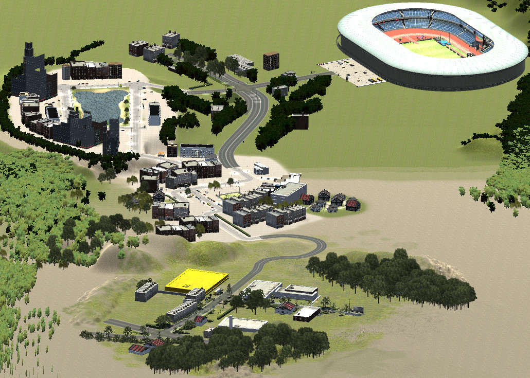
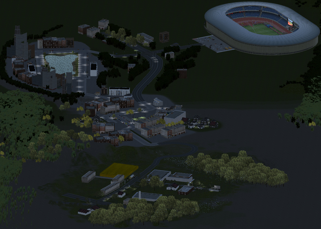
Figure 2: Orthographic view of different world regions during day and night. Time of the day affects lighting and shadows of the world, with urban lights activating at dusk and deactivating at dawn.

The related work of Matikainen et al. (2011) uses MoCap data to induce realistic motion in an “abstract armature” placed in an empty synthetic environment, generating $2,000$ short 3-second clips at $320\times 240$ and 30FPS. From these non-photo-realistic clips, handcrafted motion features are selected as relevant and later used to learn action recognition models for 11 actions in real-world videos. In contrast, our approach does not just replay MoCap, but procedurally generates new action categories – including interactions between persons, objects and the environment – as well as random physically plausible variations. Moreover, we jointly generate and learn deep representations of both action appearance and motion thanks to our realistic synthetic data, and our multi-task learning formulation to combine real and synthetic data.

An alternative to our procedural generative model that also does not require manual video labeling is the unsupervised Video Generative Adversarial Network (VGAN) of Vondrick et al. (2016) and its recent variations (Saito et al., 2017; Tulyakov et al., 2018). Instead of leveraging prior structural knowledge about physics and human actions, Vondrick et al. (2016) view videos as tensors of pixel values and learn a two-stream GAN on $5,000$ hours of unlabeled Flickr videos. This method focuses on tiny videos and capturing scene motion assuming a stationary camera. This architecture can be used for action recognition in videos when complemented with prediction layers fine-tuned on labeled videos. Compared to this approach, our proposal allows to work with any state-of-the-art discriminative architecture, as video generation and action recognition are decoupled steps. We can, therefore, benefit from a strong ImageNet initialization for both appearance and motion streams as in (Wang et al., 2016b) and network inflation as in (Carreira and Zisserman, 2017).

Moreover, in contrast to (Vondrick et al., 2016), we can decide what specific actions, scenarios, and camera-motions to generate, enforcing diversity thanks to our interpretable parametrization. While more recent works such as the Conditional Temporal GAN of Saito et al. (2017) enable certain control over which action class should be generated, they do not offer precise control over every single parameter of a scene, and neither are guaranteed to generate the chosen action in case these models did not receive sufficient training (obtaining controllable models for video generation has been an area of active research, e.g., Hao et al. (2018); Li et al. (2018); Marwah et al. (2017)). For these reasons, we show in Section 7 that, given the same amount of labeled videos, our model achieves nearly two times the performance of the unsupervised features shown in (Vondrick et al., 2016).

In general, GANs have found multiple applications for video, including face reenacting (Wu et al., 2018), generating time-lapse videos (Xiong et al., 2018), generating articulated motions (Yan et al., 2017), and human motion generation (Yang et al., 2018). From those, the works of Yan et al. (2017) and Yang et al. (2018) are able to generate articulated motions which could be readily integrated into works based on 3D game engines such as ours. Those works are therefore complimentary to ours, and we show in Section 3.3 how our system can leverage animation sequences from multiple (and possibly synthetic) sources to include even more diversity in our generated videos. Moreover, unlike approaches based on GANs, our approach has the unique advantage of being able to generate pixel-perfect ground-truth for multiple tasks besides image classification, as we show in Section 5.1.

3 Controllable virtual world

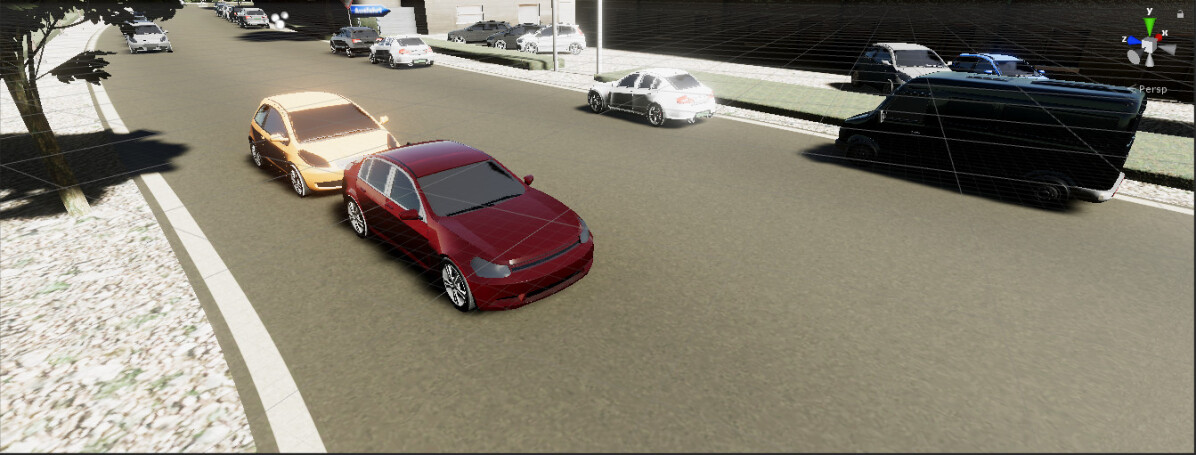
Figure 3: World location shared between PHAV and Virtual KITTI (Gaidon et al., 2016), as seen from within the Unity® editor.

In this section we describe the procedural generation techniques we leverage to randomly sample diverse yet physically plausible appearance and motion variations, both for MoCap-grounded actions and programmatically defined categories.

3.1 Action scene composition

In order to generate a human action video, we place a protagonist performing an action in an environment, under particular weather conditions at a specific period of the day. There can be one or more background actors in the scene, as well as one or more supporting characters. We film the virtual scene using a parametric camera behavior.

The protagonist is the main human model performing the action. For actions involving two or more people, one is chosen to be the protagonist. Background actors can freely walk in the current virtual environment, while supporting characters are actors with a secondary role whose performance is necessary in order to complete an action (e.g., hold hands).

The action is a human motion belonging to a predefined semantic category originated from one or more motion data sources (described in Section 3.3), including predetermined motions from a MoCap dataset, or programmatic actions defined using procedural animation techniques (Egges et al., 2008; van Welbergen et al., 2009), in particular ragdoll physics. In addition, we use these techniques to sample physically plausible motion variations (described in Section 3.4) to increase diversity.

The environment refers to a region in the virtual world (cf. Figure 2), which consists of large urban areas, natural environments (e.g., forests, lakes, and parks), indoor scenes, and sports grounds (e.g., a stadium). Each of these environments may contain moving or static background pedestrians or objects – e.g., cars, chairs – with which humans can physically interact, voluntarily or not. The outdoor weather in the virtual world can be rainy, overcast, clear, or foggy. The period of the day can be dawn, day, dusk, or night.

Similar to Gaidon et al. (2016) and Ros et al. (2016), we use a library of pre-made 3D models obtained from the Unity Asset Store, which includes artist-designed human, object, and texture models, as well as semi-automatically created realistic environments e.g., selected scenes from the Virtual KITTI dataset of Gaidon et al. (2016), cf. Figure 3.

3.2 Camera

We use a physics-based camera which we call the Kite camera (cf. Figure 4) to track the protagonist in a scene. This physics-aware camera is governed by a rigid body attached by a spring to a target position that is, in turn, attached to the protagonist by another spring. By randomly sampling different parameters for the drag and weight of the rigid bodies, as well as elasticity and length of the springs, we can achieve cameras with a wide range of shot types, 3D transformations, and tracking behaviors, such as following the actor, following the actor with a delay, or stationary.

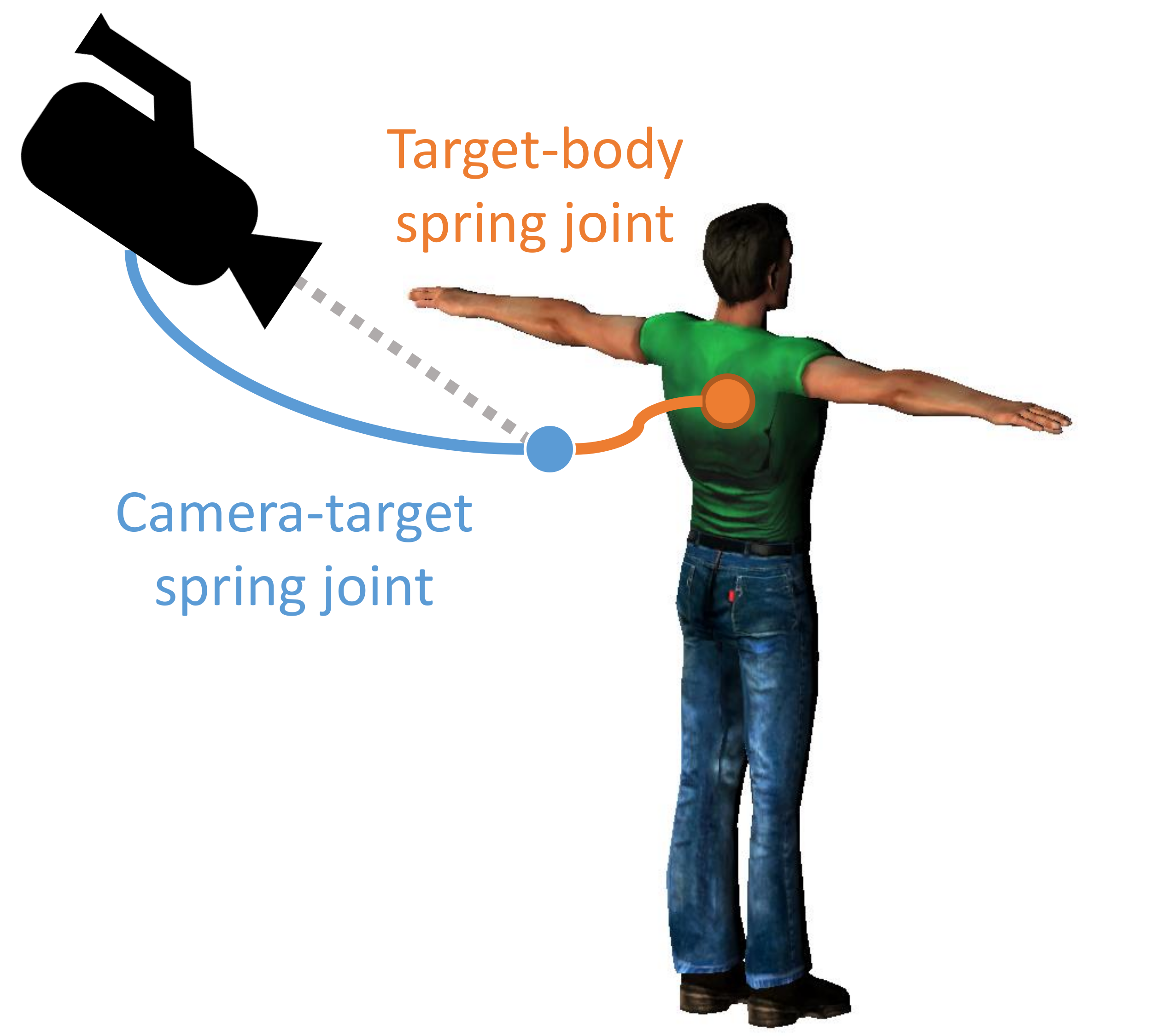
Figure 4: Representation of our Kite camera.

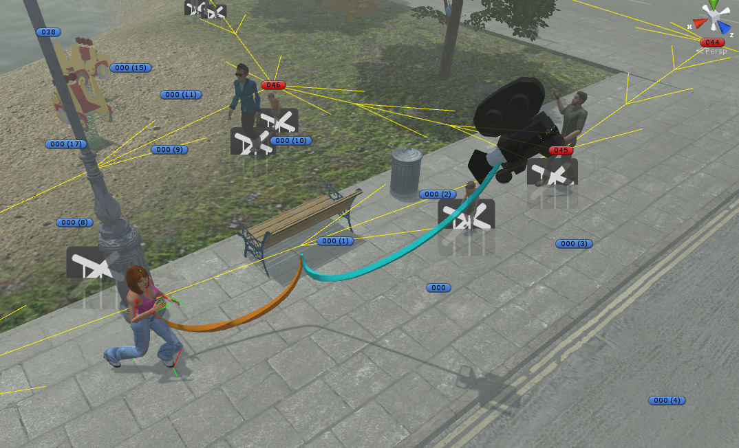
Figure 5: In-editor representation of the Kite camera. The camera is a physical object capable of interacting with other objects in the world, which avoids trespassing walls or filming from unfeasible locations. The camera focuses on a point (contact point between orange and blue cords) which is simultaneously attached to the protagonist and to the camera.

Another parameter controls the direction and strength of an initial impulse that starts moving the camera in a random direction. With different rigid body parameters, this impulse can cause our camera to simulate a handheld camera, move in a circular trajectory, or freely bounce around in the scene while filming the attached protagonist. A representation of the camera attachment in the virtual world is shown in Figure 5.

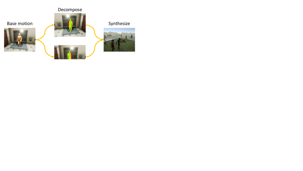
Figure 6: We decompose existing action sequences (left) into atomic motions (middle) and then recombine them into new animation sequences using procedural animation techniques, like blending and ragdoll physics. This technique can be used to both generate new motion variations for an existing action category, and to synthesize new motion sequences for entirely synthetic categories which do not exist in the data source using simple programmable rules e.g., by tying the ragdoll hands together (right). The physics engine enforces that the performed ragdoll manipulations result in physically plausible animations.

3.3 Actions

Our approach relies on two main existing data sources for basic human animations. First, we use the CMU MoCap database (Carnegie Mellon Graphics Lab, 2016), which contains 2605 sequences of 144 subjects divided in 6 broad categories, 23 subcategories and further described with a short text. We leverage relevant motions from this dataset to be used as a motion source for our procedural generation based on a simple filtering of their textual motion descriptions. Second, we use a large amount of hand-designed realistic motions made by animation artists and available on the Unity Asset Store.

The key insight of our approach is that these sources need not necessarily contain motions from predetermined action categories of interest, neither synthetic nor target real-world actions (unknown a priori). Instead, we propose to use these sources to form a library of atomic motions to procedurally generate realistic action categories. We consider atomic motions as individual movements of a limb in a larger animation sequence. For example, atomic motions in a “walk” animation include movements such as rising a left leg, rising a right leg, and pendular arm movements. Creating a library of atomic motions enables us to later recombine those atomic actions into new higher-level animation sequences, e.g., “hop” or “stagger”.

Table 3: Action categories included in PHAV.

Type	Count	Actions
sub-HMDB	21	brush hair, catch, clap, climb stairs, golf, jump, kick ball, push, pick, pour, pull up, run, shoot ball, shoot bow, shoot gun, sit, stand, swing baseball, throw, walk, wave
One-person synthetic	10	car hit, crawl, dive floor, flee, hop, leg split, limp, moonwalk, stagger, surrender
Two-people synthetic	4	walking hug, walk holding hands, walk the line, bump into each other

Our PHAV dataset contains 35 different action classes (cf. Table 3), including 21 simple categories present in HMDB-51 and composed directly of some of the aforementioned atomic motions. In addition to these actions, we programmatically define 10 action classes involving a single actor and 4 action classes involving two person interactions. We create these new synthetic actions by taking atomic motions as a base and using procedural animation techniques like blending and ragdoll physics (cf. Section 3.4) to compose them in a physically plausible manner according to simple rules defining each action, such as tying hands together (e.g., “walk hold hands”, cf. Figure 6), disabling one or more muscles (e.g., “crawl”, “limp”), or colliding the protagonist against obstacles (e.g., “car hit”, “bump into each other”).

3.4 Physically plausible motion variations

We now describe procedural animation techniques (Egges et al., 2008; van Welbergen et al., 2009) to randomly generate large amounts of physically plausible and diverse human action videos, far beyond what can be achieved by simply replaying atomic motions from a static animation source.

Ragdoll physics.

A key component of our work is the use of ragdoll physics. Ragdoll physics are limited real-time physical simulations that can be used to animate a model (e.g., a human model) while respecting basic physics properties such as connected joint limits, angular limits, weight and strength. We consider ragdolls with 15 movable body parts (referenced herein as muscles), as illustrated in Figure 7. For each action, we separate those 15 muscles into two disjoint groups: those that are strictly necessary for performing the action, and those that are complementary (altering their movement should not interfere with the semantics of the currently considered action). The ragdoll allows us to introduce variations of different nature in the generated samples. The other modes of variability generation described in this section will assume that the physical plausibility of the models is being kept by the use of ragdoll physics. We use RootMotion’s PuppetMaster for implementing and controlling human ragdolls in Unity® Pro.

Random perturbations.

Inspired by Perlin (1995), we create variations of a given motion by adding random perturbations to muscles that should not alter the semantic category of the action being performed. Those perturbations are implemented by adding a rigid body to a random subset of the complementary muscles. Those bodies are set to orbit around the muscle’s position in the original animation skeleton, drifting the movement of the puppet’s muscle to its own position in a periodic oscillating movement. More detailed references on how to implement variations of this type can be found in  (Perlin, 1995; Egges et al., 2008; Perlin and Seidman, 2008; van Welbergen et al., 2009) and references therein.

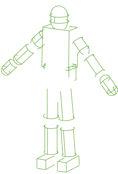
Figure 7: Ragdoll configuration with 15 muscles.

Muscle weakening.

We vary the strength of the avatar performing the action. By reducing its strength, the actor performs an action with seemingly more difficulty.

Action blending.

Similarly to modern video games, we use a blended ragdoll technique to constrain the output of a pre-made animation to physically plausible motions. In action blending, we randomly sample a different motion sequence (coming either from the same or from a different action class, which we refer to as the base motion) and replace the movements of current complementary muscles with those from this new sequence. We limit the number of blended sequences in PHAV to be at most two.

Objects.

The last physics-based source of variation is the use of objects. First, we manually annotated a subset of the MoCap actions marking the instants in time where the actor started or ended the manipulation of an object. Second, we use inverse kinematics to generate plausible programmatic interactions.

Table 4: Overview of key random variables of our generative model of human action videos .

Parameter	Variable	Count	Possible values
Human Model	H	20	models designed by artists
Environment	E	7	simple, urban, green, middle, lake, stadium, house interior
Weather	W	4	clear, overcast, rain, fog
Period of day	D	4	night, dawn, day, dusk
Variation	V	5	none, muscle perturbation, muscle weakening, action blending, objects

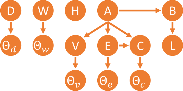
Figure 8: A simplified view of the graphical model for our generator (cf. Section 4.2 for the meaning of each variable). A complete and more detailed version is shown in Figure 9.

4 Generative models for world control

In this section we introduce our interpretable parametric generative model of videos depicting particular human actions, and show how we use it to generate our PHAV dataset. We start by providing a simplified version of our model (cf.  Figure 8), listing the main variables in our approach, and giving an overview of how our model is organized. After this brief overview, we show our complete model (cf.  Figure 9) and describe its multiple components in detail.

4.1 Overview

We define a human action video as a random variable:

$$X=\left\langle H,A,L,B,V,C,E,D,W\right\rangle$$ (1)

where $H$ is a human model, $A$ an action category, $L$ a video length, $B$ a set of basic motions (from MoCap, manual design, or programmed), $V$ a set of motion variations, $C$ a camera, $E$ an environment, $D$ a period of the day, $W$ a weather condition, and possible values for those parameters are shown in Table 4. Given this definition, a simplified version for our generative model (cf.  Figure 8) for an action video $X$ can then be given by:

$$P(X)= P(H)\leavevmode\nobreak\ P(A)\leavevmode\nobreak\ P(L\mid B)\leavevmode\nobreak\ P(B\mid A)$$ (2)

$$P(\Theta_{v}\mid V)\leavevmode\nobreak\ P(V\mid A)$$

$$P(\Theta_{e}\mid E)\leavevmode\nobreak\ P(E\mid A)$$

$$P(\Theta_{c}\mid C)\leavevmode\nobreak\ P(C\mid A,E)$$

$$P(\Theta_{d}\mid D)\leavevmode\nobreak\ P(D)$$

$$P(\Theta_{w}\mid W)\leavevmode\nobreak\ P(W)$$

where $\Theta_{w}$ is a random variable on weather-specific parameters (e.g., intensity of rain, clouds, fog), $\Theta_{c}$ is a random variable on camera-specific parameters (e.g., weights and stiffness for Kite camera springs), $\Theta_{e}$ is a random variable on environment-specific parameters (e.g., current waypoint, waypoint locations, background pedestrian starting points and destinations), $\Theta_{d}$ is a random variable on period-specific parameters (e.g., amount of sunlight, sun orientation), and $\Theta_{v}$ is a random variable on variation-specific parameters (e.g., strength of each muscle, strength of perturbations, blending muscles). The probability functions associated with categorical variables (e.g., $A$) can be either uniform, or configured manually to use pre-determined weights. Similarly, probability distributions associated with continuous values (e.g., $\Theta_{c}$) are either set using a uniform distribution with finite support, or using triangular distributions with pre-determined support and most likely value.

4.2 Variables

We now proceed to define the complete version of our generative model. We start by giving a more precise definition for its main random variables. Here we focus only on critical variables that are fundamental in understanding the orchestration of the different parts of our generation, whereas all part-specific variables are shown in Section 4.3. The categorical variables that drive most of the procedural generation are:

$$H :h\in \leavevmode\nobreak\ \{{model}_{1},{model}_{2},\dots,{model}_{20}\}$$ (3)

$$A :a\in \leavevmode\nobreak\ \{clap,\dots,bump\leavevmode\nobreak\ into\leavevmode\nobreak\ each\leavevmode\nobreak\ other\}$$

$$B :b\in \leavevmode\nobreak\ \{{motion}_{1},{motion}_{2},\dots,{motion}_{862}\}$$

$$V :v\in \leavevmode\nobreak\ \{none,random\leavevmode\nobreak\ perturbation,$$

$$\leavevmode\nobreak\ \leavevmode\nobreak\ weakening,objects,blend\}$$

$$C :c\in \leavevmode\nobreak\ \{kite,indoors,closeup,static\}$$

$$E :e\in \leavevmode\nobreak\ \{urban,stadium,middle,$$

$$\leavevmode\nobreak\ \leavevmode\nobreak\ green,house,lake\}$$

$$D :d\in \leavevmode\nobreak\ \{dawn,day,dusk,night\}$$

$$W :w\in \leavevmode\nobreak\ \{clear,overcast,rain,fog\}$$

where $H$ is the human model to be used by the protagonist, $A$ is the action category for which the video should be generated, $B$ is the motion sequence (e.g., from MoCap, created by artists, or programmed) to be used as a base upon which motion variations can be applied (e.g., blending it with secondary motions), $V$ is the motion variation to be applied to the base motion, $C$ is the camera behavior, $E$ is the environment of the virtual world where the action will take place, $D$ is the day phase, and $W$ is the weather condition.

These categorical variables are in turn controlled by a group of parameters that can be adjusted in order to drive the sample generation. These parameters include the $\bm{\theta_{A}}$ parameters of a categorical distribution on action categories $A$, the $\bm{\theta_{W}}$ for weather conditions $W$, $\bm{\theta_{D}}$ for day phases $D$, $\bm{\theta_{H}}$ for model models $H$, $\bm{\theta_{V}}$ for variation types $V$, and $\bm{\theta_{C}}$ for camera behaviors $C$.

Additional parameters include the conditional probability tables of the dependent variables: a matrix of parameters $\bm{\theta_{AE}}$ where each row contains the parameters for categorical distributions on environments $E$ for each action category $A$, the matrix of parameters $\bm{\theta_{AC}}$ on camera behaviors $C$ for each action $A$, the matrix of parameters $\bm{\theta_{EC}}$ on camera behaviors $C$ for each environment $E$, and the matrix of parameters $\bm{\theta_{AB}}$ on motions $B$ for each action $A$.

Finally, other relevant parameters include $T_{min}$, $T_{max}$, and $T_{mod}$, the minimum, maximum and most likely durations for the generated video. We denote the set of all parameters in our model by $\bm{\theta}$.

4.3 Model

The complete interpretable parametric probabilistic model used by our generation process, given our generation parameters $\bm{\theta}$, can be written as:

$$P(H, A,L,B,V,C,E,D,W\mid\bm{\theta})=$$ (4)

$$\leavevmode\nobreak\ \leavevmode\nobreak\ P_{1}(D,W\mid\bm{\theta})\leavevmode\nobreak\ \leavevmode\nobreak\ P_{2}(H\mid\bm{\theta})$$

$$\leavevmode\nobreak\ \leavevmode\nobreak\ P_{3}(A,L,B,V,C,E,W\mid\bm{\theta})$$

where $P_{1}$, $P_{2}$ and $P_{3}$ are defined by the probabilistic graphical models represented on Figure 9(a), 9(b) and 9(c), respectively. We use extended plate notation (Bishop, 2006) to indicate repeating variables, marking parameters (non-variables) using filled rectangles.

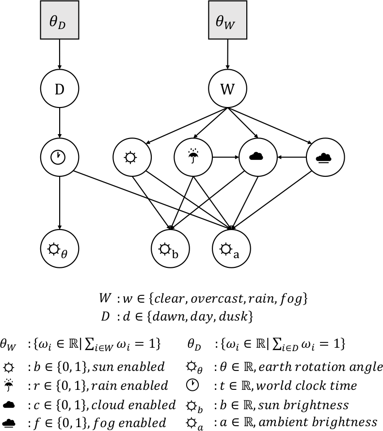
(a) Probabilistic graphical model for $P_{1}(D,W\mid\bm{\theta})$, the first part of our parametric generator (world time and weather).

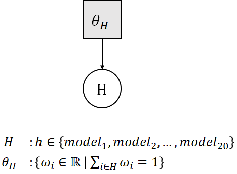
(b) Probabilistic graphical model for $P_{2}(H\mid\bm{\theta})$, the second part of our parametric generator (human models).

(c) Probabilistic graphical model for $P_{3}(A,L,B,V,C,E,W\mid\bm{\theta})$, the third part of our parametric generator (scene and action preparation).

Figure 9: Our complete probabilistic graphical model, divided in three parts.

4.4 Distributions

The generation process makes use of four main families of distributions: categorical, uniform, Bernoulli and triangular. We adopt the following three-parameter formulation for the triangular distribution:

$$Tr(x\mid a,b,c)=\begin{cases}0&\text{for }x<a,\\ \frac{2(x-a)}{(b-a)(c-a)}&\text{for }a\leq x<c,\\[4.0pt] \frac{2}{b-a}&\text{for }x=c,\\[4.0pt] \frac{2(b-x)}{(b-a)(b-c)}&\text{for }c<x\leq b,\\[4.0pt] 0&\text{for }b<x.\end{cases}$$ (5)

All distributions are implemented using the open-source Accord.NET Framework (De Souza, 2014). While we have used mostly uniform distributions to create the dataset used in our experiments, we have the possibility to bias the generation towards values that are closer to real-world dataset statistics.

Day phase.

As real-world action recognition datasets are more likely to contain video recordings captured during daylight, we fixed the parameter $\bm{\theta_{D}}$ such that:

$$P(D= \leavevmode\nobreak\ dawn \mid\bm{\theta_{D}}) = \nicefrac{{1}}{{3}}$$ (6)

$$P(D= \leavevmode\nobreak\ day \mid\bm{\theta_{D}}) = \nicefrac{{1}}{{3}}$$

$$P(D= \leavevmode\nobreak\ dusk \mid\bm{\theta_{D}}) = \nicefrac{{1}}{{3}}$$

$$P(D= \leavevmode\nobreak\ night \mid\bm{\theta_{D}}) = 0$$ .

We note that although our system can also generate night samples, we do not include them in PHAV at this moment to reflect better the contents of real world datasets.

Weather.

In order to support a wide range of applications of our dataset, we fixed the parameter $\bm{\theta_{W}}$ such that:

$$P(W= \leavevmode\nobreak\ clear \mid\bm{\theta_{W}}) = \nicefrac{{1}}{{4}}$$ (7)

$$P(W= \leavevmode\nobreak\ overcast \mid\bm{\theta_{W}}) = \nicefrac{{1}}{{4}}$$

$$P(W= \leavevmode\nobreak\ rain \mid\bm{\theta_{W}}) = \nicefrac{{1}}{{4}}$$

$$P(W= \leavevmode\nobreak\ fog \mid\bm{\theta_{W}}) = \nicefrac{{1}}{{4}}$$ ,

ensuring all weather conditions are present.

Camera.

In addition to the Kite camera, we also included specialized cameras that can be enabled only for certain environments (Indoors), and certain actions (Close-Up). We fixed the parameter $\bm{\theta_{C}}$ such that:

$$P(C= \leavevmode\nobreak\ kite \mid\bm{\theta_{C}}) = \nicefrac{{1}}{{3}}$$ (8)

$$P(C= \leavevmode\nobreak\ closeup \mid\bm{\theta_{C}}) = \nicefrac{{1}}{{3}}$$

$$P(C= \leavevmode\nobreak\ indoors \mid\bm{\theta_{C}}) = \nicefrac{{1}}{{3}}$$ .

However, we have also fixed $\bm{\theta_{CE}}$ and $\bm{\theta_{AC}}$ such that the Indoors camera is only available for the house environment, and that the Close-Up camera can also be used for the BrushHair action in addition to Kite.

Environment, human model and variations.

We fixed the parameters $\bm{\theta_{E}}$, $\bm{\theta_{H}}$, and $\bm{\theta_{V}}$ using equal weights, such that the variables $E$, $H$, and $V$ can have uniform distributions.

Base motions.

We select a main motion sequence which will be used as a base upon which a variation $V$ is applied (cf. Section 4.2). Base motions are weighted according to the minimum video length parameter $T_{min}$, where motions whose duration is less than $T_{min}$ are assigned weight zero, and others are set to uniform, such that:

$$P(B=b|T_{min})\propto\begin{cases}1&\text{if }length(b)\geq T_{min}\\ 0&\text{otherwise}\\ \end{cases}.$$ (9)

This weighting is used to ensure that the motion that will be used as a base is long enough to fill the minimum desired duration for a video. We then perform the selection of a motion $B$ given a category $A$ by introducing a list of regular expressions associated with each of the action categories. We then compute matches between the textual description of the motion in its source, e.g., short text descriptions by Carnegie Mellon Graphics Lab (2016), and these expressions, such that:

$$(\bm{\theta_{AB}})_{ab}=\begin{cases}1&\text{if }match(\text{regex}_{a},\text{desc}_{b})\\ 0&\text{otherwise}\\ \end{cases}$$ (10)

$$\forall a\in A,\forall b\in B.$$

We then define $\bm{\theta_{AB}}$ such that:

$$P(B=b\mid A=a,\bm{\theta_{AB}})\propto(\bm{\theta_{AB}})_{a,b}.\\$$ (11)

In this work, we use 859 motions from MoCap and 3 designed by animation artists. These 862 motions then serve as a base upon which the procedurally defined (i.e. composed motions based on programmable rules, cf. Figure 6) and procedurally generated (i.e. motions whose end result will be determined by the value of other random parameters and their effects and interactions during the runtime, cf. Section 3.4) are created. In order to make the professionally designed motions also searchable by Eq.(10), we also annotate them with small textual descriptions.

Weather elements.

The selected weather $W$ affects world parameters such as the sun brightness, ambient luminosity, and multiple boolean variables that control different aspects of the world (cf. Figure 9(a)). The activation of one of these boolean variables (e.g., fog visibility) can influence the activation of others (e.g., clouds) according to Bernoulli distributions ($p=0.5$).

World clock time.

The world time is controlled depending on $D$. In order to avoid generating a large number of samples in the borders between two periods of the day, where the distinction between both phases is blurry, we use different triangular distributions associated with each phase, giving a larger probability to hours of interest (sunset, dawn, noon) and smaller probabilities to hours at the transitions. We therefore define the distribution of the world clock times $P(T)$ as:

$$P(T=t\mid D)\propto\sum_{d\in D}P(T=t\mid D=d)$$ (12)

where:

$$P(T=t\mid D= dawn) =Tr(t\mid 7h,10h,9h)$$ (13)

$$P(T=t\mid D= day) =Tr(t\mid 10h,16h,13h)$$

$$P(T=t\mid D= dusk) =Tr(t\mid 17h,20h,18h)$$

$$P(T=t\mid D= night )=Tr(t\mid 20h,7h,0h).$$

Generated video duration.

The selection of the clip duration $L$ given the selected motion $b$ is performed considering the motion length $L_{b}$, the maximum video length $T_{min}$ and the desired mode $T_{mod}$:

$$P(L=l\mid B=b)=Tr( a=T_{min},$$ (14)

$$b=min(L_{b},T_{max}),$$

$$c=min(T_{mod},L_{b})).$$

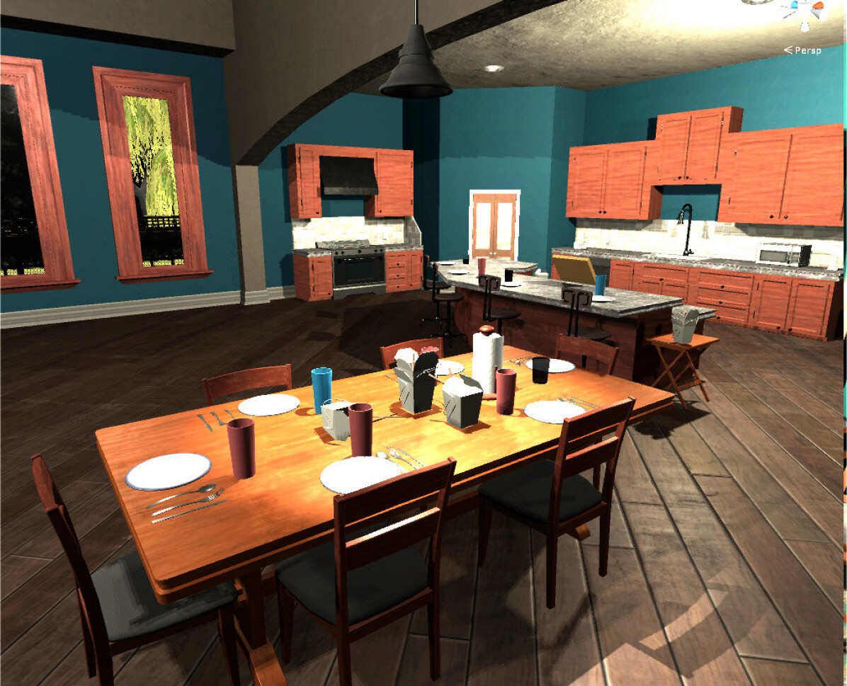
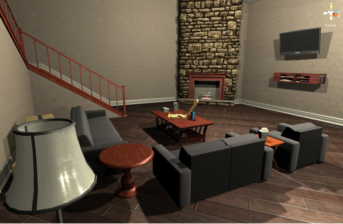
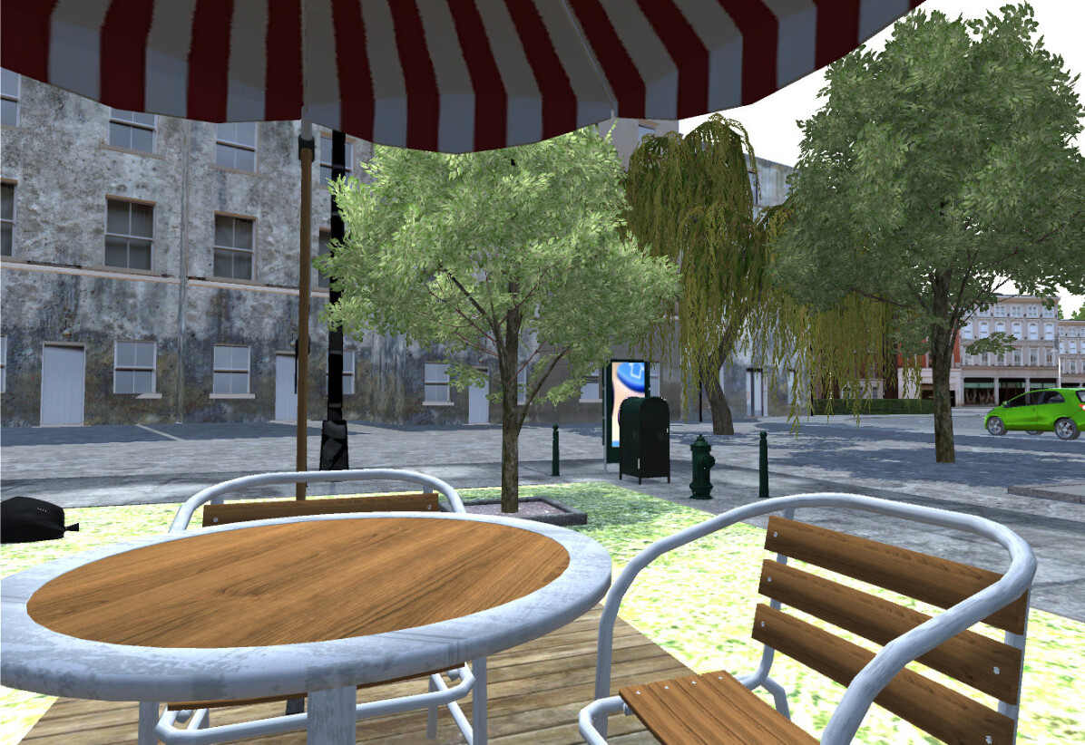
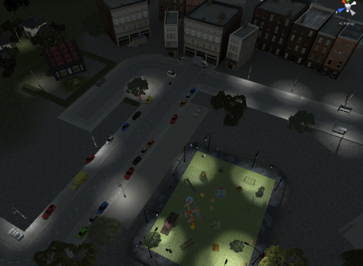
Figure 10: Examples of indoor (top) and outdoor (bottom) locations in PHAV.

Actors placement and environment.

Each environment $E$ has at most two associated waypoint graphs. One graph refers to possible positions for the protagonist, while an additional second graph gives possible positions $B_{WG}$ for spawning background actors. Indoor scenes (cf. Figure 10) do not include background actor graphs. After an environment has been selected, a waypoint $P_{W}$ is randomly selected from the graph using a uniform distribution. The protagonist position $P_{xyz}$ is then set according to the position of $P_{W}$. The $S_{xyz}$ position of each supporting character, if any, is set depending on $P_{xyz}$. The position and destinations for the background actors are set depending on $B_{WG}$.

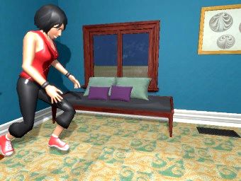
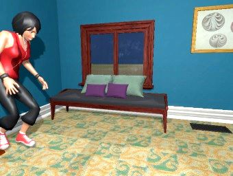
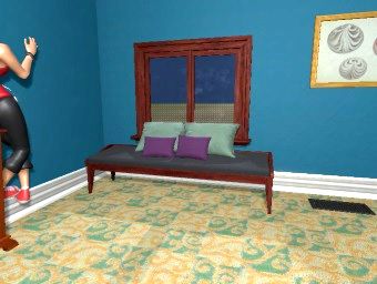
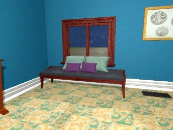
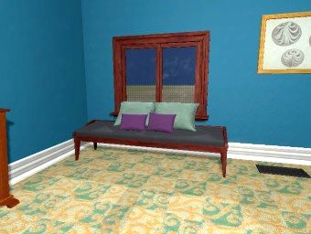
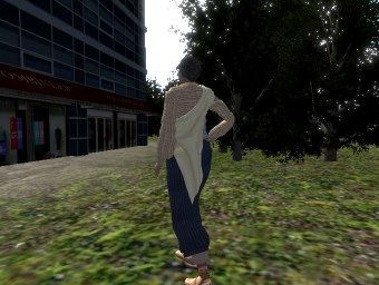
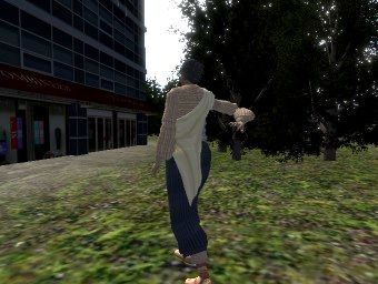
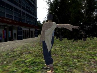
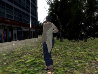
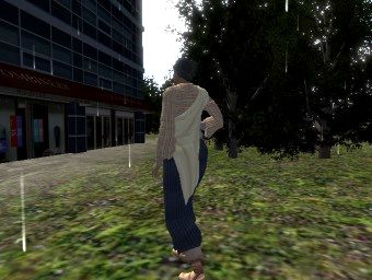
Figure 11: Example generation failure cases. First row: too strong perturbations (small model, brushing hair looks like dancing). Second row: limitation in the physics engine together with ragdoll system and MoCap action can lead to physics violations (passing through a wall). Third row: problems in the automatic configuration of the ragdoll model can result in overconstrained joints and unintended variations.

Camera placement and parameters.

After a camera has been selected, its position $C_{xyz}$ and the position $T_{xyz}$ of the target are set depending on the position $P_{xyz}$ of the protagonist. The camera parameters are randomly sampled using uniform distributions on sensible ranges according to the observed behavior in Unity®. The most relevant secondary variables for the camera are shown in Figure 9(c). They include Unity-specific parameters for the camera-target ($CT_{s}$, $CT_{m}$) and target-protagonist springs ($TP_{s}$, $CT_{m}$) that can be used to control their strength and a minimum distance tolerance zone in which the spring has no effect (remains at rest). In our generator, the minimum distance is set to either 0, 1 or 2 meters with uniform probabilities. This setting is responsible for a “delay” effect that allows the protagonist to not be always in the center of camera focus (and thus avoiding creating such bias in the data).

Action variations.

After a variation mode has been selected, the generator needs to select a subset of the ragdoll muscles (cf. Figure 7) to be perturbed (random perturbations) or to be replaced with movement from a different motion (action blending). These muscles are selected using a uniform distribution on muscles that have been marked as non-critical depending on the previously selected action category $A$. When using weakening, a subset of muscles will be chosen to be weakened with varying parameters independent of the action category. When using objects, the choice of objects to be used and how they have to be used is also dependent on the action category.

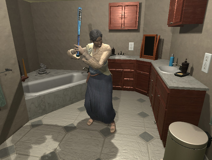
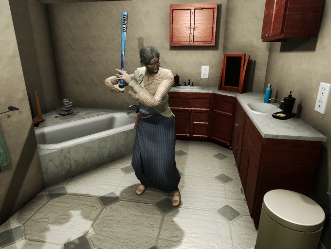
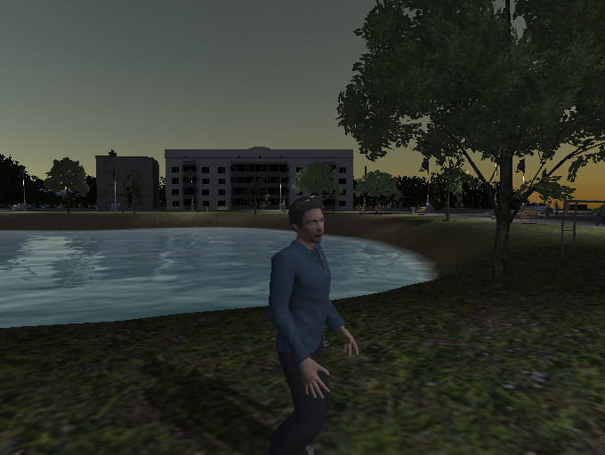
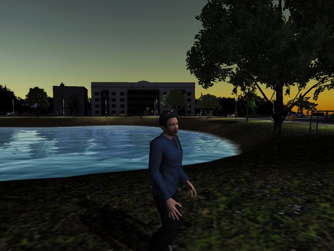
Figure 12: Comparison between raw (left) vs. post-processed (right) RGB frames.

Failure cases.

Although our approach uses physics-based procedural animation techniques, unsupervised generation of large amounts of random variations with a focus on diversity inevitably causes edge cases where physical models fail. This results in glitches reminiscent of typical video game bugs (cf. Figure 11). Using a random $1\%$ sample of our dataset, we manually estimated that this corresponds to less than $10\%$ of the videos generated. While this could be improved, our experiments in Section 7 show that the accuracy of neural network models do increase when trained with this data. We also compare our results to an earlier version of this dataset with an increased level of noise and show it has little to no effect in terms of final accuracy in real-world datasets.

5 Generating a synthetic action dataset

We validate our approach for synthetic video generation by generating a new dataset for action recognition, such that the data from this dataset could be used to complement the training set of existing target real-world datasets in order to obtain action classification models which perform better in their respective real-world tasks. In this section we give details about how we have used the aforedescribed model to generate our PHAV dataset.

In order to create PHAV, we generate videos with lengths between 1 and 10 seconds, at 30 FPS, and resolution of $340\times 256$ pixels, as this is the same resolution expected by recent action recognition models such as (Wang et al., 2016b). We use anti-aliasing, motion blur, and standard photo-realistic cinematic effects (cf. Figure 12). We have generated $55$ hours of videos, with approximately $6M$ frames and at least $1,000$ videos per action category.

Our parametric model can generate fully-annotated action videos (including depth, flow, semantic segmentation, and human pose ground-truths) at 3.6 FPS using one consumer-grade gaming GPU (NVIDIA GTX 1070). In contrast, the average annotation time for data-annotation methods such as (Richter et al., 2016; Cordts et al., 2016; Brostow et al., 2009) are significantly below 0.5 FPS. While those works deal with semantic segmentation (where the cost of annotation is higher than for action classification), we can generate all modalities for roughly the same cost as RGB using Multiple Render Targets (MRT).

Multiple Render Targets.

This technique allows for a more efficient use of the GPU by grouping together multiple draw calls of an object into a single call. The standard approach to generate multiple image modalities for the same object is to perform multiple rendering passes over the same object with variations of their original shaders that output the data modalities we are interested in (e.g., the semantic segmentation ground-truth for an object would be obtained by replacing the standard texture shader used by each object in the scene with a shader that can output a constant color without any light reflection effects).

However, replacing shaders for every ground-truth is also an error prone process. Certain objects with complex geometry (e.g.,  tree leaves) require special complex vertex and geometry shaders which would need to be duplicated for each different modality. This increase in the number of shaders also increases the chances of designer- and programmer-error when replacing shaders of every object in a scene with shaders that support different ground-truths.

On the other hand, besides being more efficient, the use of MRT allows us to concentrate the generation of multiple outputs at the definition of a single shader, removing the hurdle of having to switch shaders during both design- and run-time. In order to use this technique, we modify Unity®’s original shader definitions. For every shader, we alter the fragment shader at their final rendering pass to generate, alongside RGB, all the extra visual modalities we mention next.

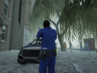
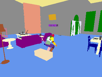
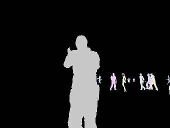
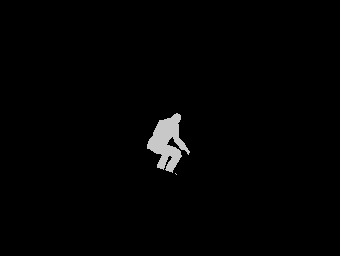
Figure 14: Example frames and data modalities for a synthetic action (car hit, left) and MoCap-based action (sit, right). From top to bottom: Rendered RGB Frames, Semantic Segmentation, Instance Segmentation, Depth Map, Horizontal Optical Flow, and Vertical Optical Flow. Depth image brightness has been adjusted in this figure to ensure visibility on paper.

5.1 Data modalities

Our generator outputs multiple data modalities for a single video, which we include in our public release of PHAV (cf. Figure 14). Those data modalities are rendered roughly at the same time using MRT, resulting in a superlinear speedup as the number of simultaneous output data modalities grows. The modalities in our public release include:

Rendered RGB Frames.

These are the RGB frames that constitute the action video. They are rendered at $340\times 256$ resolution and 30 FPS such that they can be directly fed to two-stream style networks. Those frames have been post-processed with 2x Supersampling Anti-Aliasing (SSAA) (Molnar, 1991; Carter, 1997), motion blur (Steiner, 2011), bloom (Steiner, 2011), ambient occlusion (Ritschel et al., 2009; Miller, 1994; Langer and Bülthoff, 2000), screen space reflection (Sousa et al., 2011), color grading (Selan, 2012), and vignette (Zheng et al., 2009).

Semantic Segmentation.

These are the per-pixel semantic segmentation ground-truths containing the object class label annotations for every pixel in the RGB frame. They are encoded as sequences of 24-bpp PNG files with the same resolution as the RGB frames. We provide 63 pixel classes (cf. Table 10 in Appendix A), which include the same 14 classes used in Virtual KITTI (Gaidon et al., 2016), classes specific for indoor scenarios, classes for dynamic objects used in every action, and 27 classes depicting body joints and limbs (cf. Figure 15).

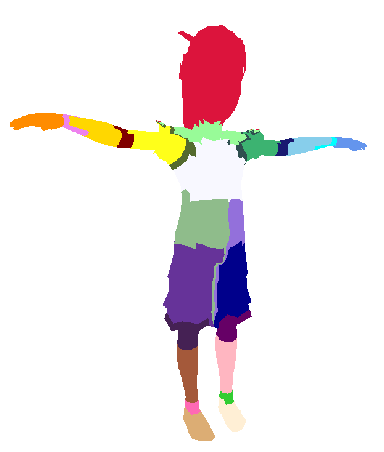
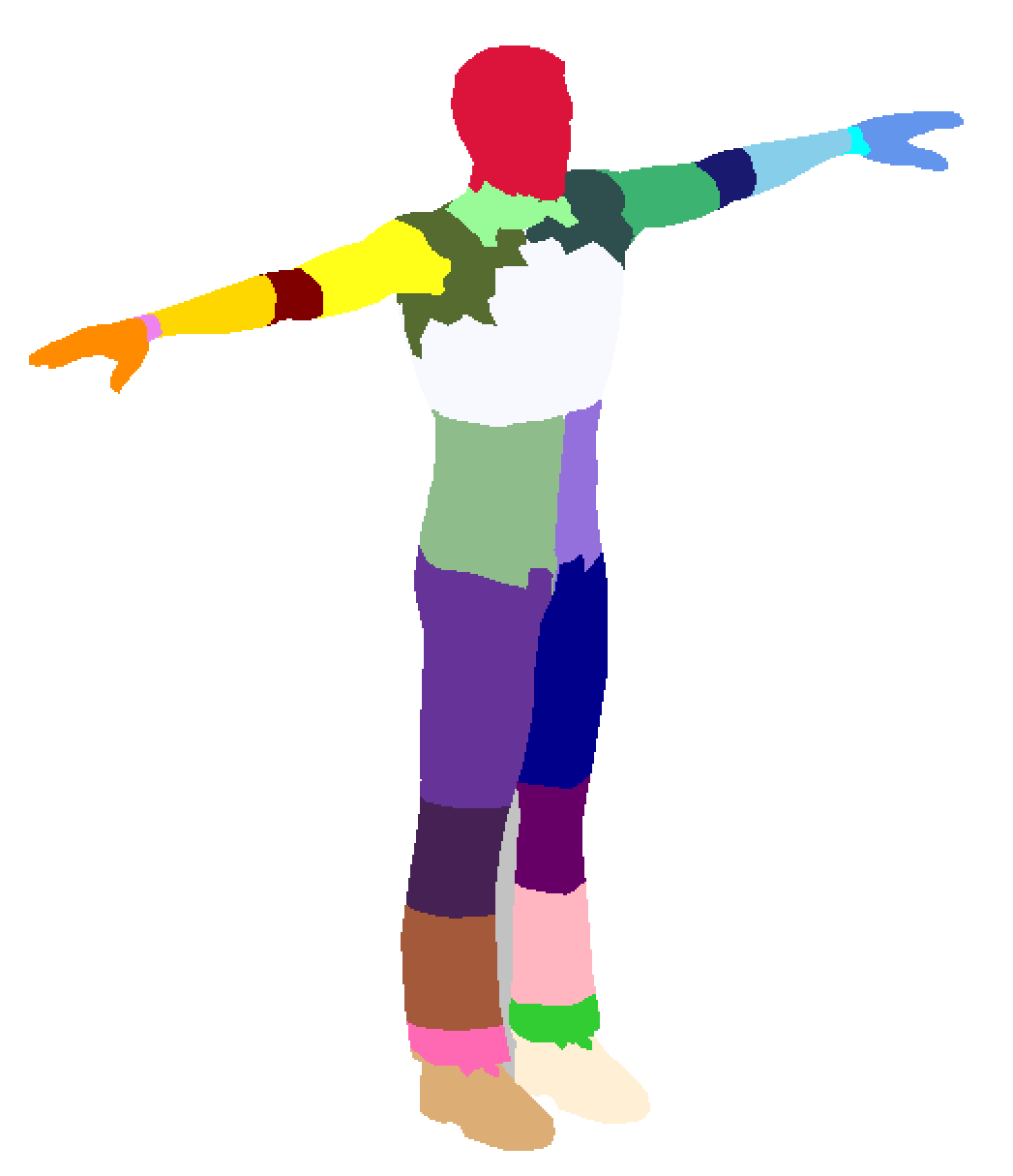
Figure 15: Semantic segmentation ground-truth for human bodies in PHAV. In order to make our approach scalable, body segments are determined automatically for every model through a series of line and distance tests with models in a standardized key position. The spatial resolution of the segments are determined by the resolution of their meshes.

Instance Segmentation.

These are the per-pixel instance segmentation ground-truths containing the person identifier encoded as different colors in a sequence of frames. They are encoded in exactly the same way as the semantic segmentation ground-truth explained above.

Depth Map.

These are depth map ground-truths for each frame. They are represented as a sequence of 16-bit grayscale PNG images with a fixed far plane of 655.35 meters. This encoding ensures that a pixel intensity of 1 can correspond to a 1cm distance from the camera plane.

Optical Flow.

These are the ground-truth (forward) optical flow fields computed from the current frame to the next frame. We provide separate sequences of frames for the horizontal and vertical directions of optical flow represented as sequences of 16-bpp JPEG images with the same resolution as the RGB frames. We provide the forward version of the optical flow field in order to ensure that models based on the Two-Stream Networks of Simonyan and Zisserman (2014) could be readily applicable to our dataset, since this is the optical flow format they have been trained with (forward TV-$\ell_{1}$). However, this poses a challenge from the generation perspective. In order to generate frame $t$ one must know frame $t+1$ ahead of time. In order to achieve this, we store every transformation matrix from all objects in the virtual scene from frame $t$, and then change all vertex and geometry shaders of all shaders to return both the previous and current positions.

Raw RGB Frames.

These are the raw RGB frames before any of the post-processing effects mentioned above are applied. This modality is mostly included for completeness, and has not been used in experiments shown in this work.

Pose, location and additional information.

Although not an image modality, our generator also produces extended metadata for every frame. This metadata includes camera parameters, 3D and 2D bounding boxes, joint locations in screen coordinates (pose), and muscle information (including muscular strength, body limits and other physical-based annotations) for every person in a frame.

Procedural Video Parameters.

We also include the internal state of our generator and virtual world at the beginning of the data generation process of each video. This data can be seen as large, sparse vectors that determine the content of a procedurally generated video. These vectors contain the values of all possible parameters in our video generation model, including detailed information about roughly every rigid body, human characters, the world, and otherwise every controllable variable in our virtual scene, including the random seed which will then influence how those values will evolve during the video execution. As such, these vectors include variables that are discrete (e.g., visibility of the clouds), continuous (e.g., x-axis position of the protagonist), piecewise continuous (e.g., time of the day), and angular (e.g., rotation of the Earth). These vectors can therefore be seen as procedural recipes for each of our generated videos.

5.2 Statistics

In this section we show and discuss some key statistics for the dataset we generate, PHAV. A summary of those statistics can be seen in Table 5. Compared to UCF-101 and HMDB-51 (cf. Tables 1 and 2), we provide at least one order of magnitude more videos per categories than these datasets, supplying about $3\times$ more RGB frames in total. Considering that we provide 6 different visual data modalities, our release contains a total of  36K images ready to be used for a variety of tasks.

A detailed view of the number of videos generated for each action class is presented in Figure 17. As can be seen, the number is higher than 1,000 samples for all categories.

We also show the number of videos generated by value of each main random generation variable in Figure 16, demonstrating these histograms reflect the probability values presented in Section 4.4. We also note that, while our parametric model is flexible enough to generate a wide range of world variations, we have focused on generating videos that would be more similar to those in the target datasets.

Table 5: Statistics of PHAV.

Statistic	Value
Total dataset clips	39,982
Total dataset frames	5,996,286
Total dataset duration	2d07h31m
Average video duration	4.99s
Average number of frames	149.97
Frames per second	30
Video width	340
Video height	256
Average clips per category	1,142.3
Image modalities (streams)	6

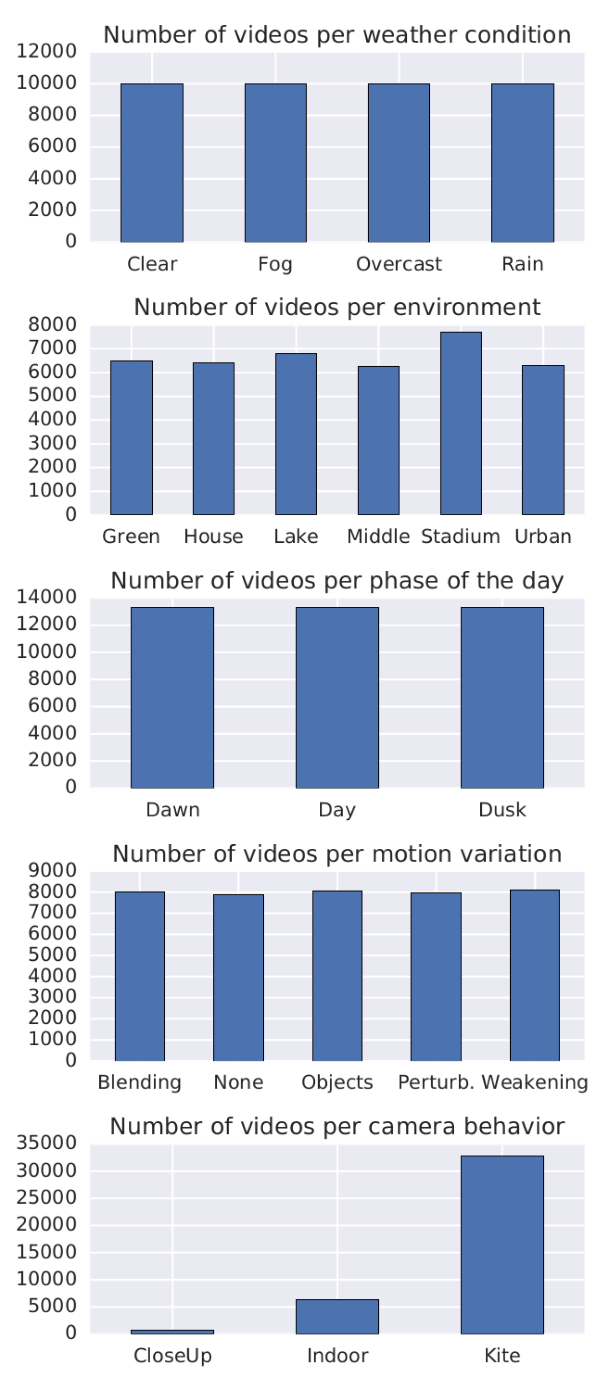
Figure 16: Number of videos per parameter value for multiple variables defined in Section 4: weather, environment, phase of the day, motion variation, and camera behavior.

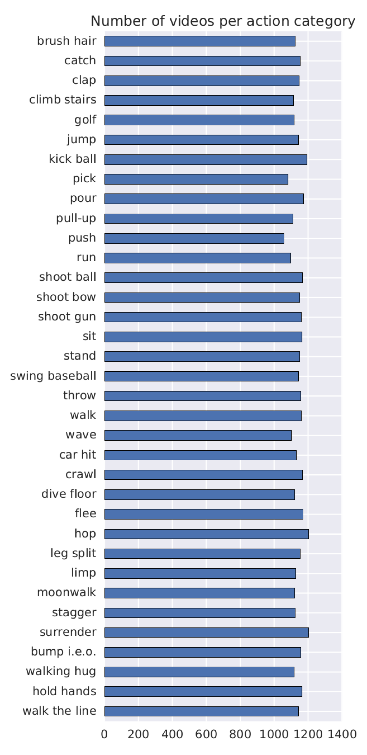
Figure 17: Plot of the number of videos generated for each category in PHAV (cf. Table 3). As can be seen, the number is higher than 1,000 samples for all categories.

6 Cool Temporal Segment Networks

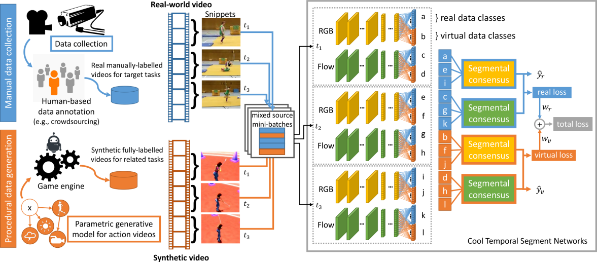
Figure 18: Our “Cool-TSN” deep multi-task learning architecture for action recognition in videos.

We propose to demonstrate the usefulness of our PHAV dataset via deep multi-task representation learning. Our main goal is to learn an end-to-end action recognition model for real-world target categories by combining a few examples of labeled real-world videos with a large number of procedurally generated videos for different surrogate categories. Our hypothesis is that, although the synthetic examples differ in statistics and tasks, their realism, quantity, and diversity can act as a strong prior and regularizer against overfitting, towards data-efficient representation learning that can operate with few manually labeled real videos. Figure 18 depicts our learning algorithm inspired by Simonyan and Zisserman (2014), but adapted for the Temporal Segment Networks (TSN) of Wang et al. (2016b) with the “cool worlds” of Vázquez et al. (2011), i.e. mixing real and virtual data during training.

6.1 Temporal Segment Networks

The recent TSN architecture of Wang et al. (2016b) improves significantly on the original two-stream architecture of Simonyan and Zisserman (2014). It processes both RGB frames and stacked optical flow frames using a deeper Inception architecture (Szegedy et al., 2015) with Batch Normalization (Ioffe and Szegedy, 2015) and DropOut Srivastava et al. (2014). Although it still requires massive labeled training sets, this architecture is more data efficient, and therefore more suitable for action recognition in videos. In particular, Wang et al. (2016b) shows that both the appearance and motion streams of TSNs can benefit from a strong initialization on ImageNet, which is one of the main factors responsible for the high recognition accuracy of TSN.

Another improvement of TSN is the explicit use of long-range temporal structure by jointly processing random short snippets from a uniform temporal subdivision of a video. TSN computes separate predictions for $K$ different temporal segments of a video. These partial predictions are then condensed into a video-level decision using a segmental consensus function $\mathbf{G}$. We use the same parameters as Wang et al. (2016b): a number of segments $K=3$, and the consensus function

$$\small\mathbf{G}=\frac{1}{K}\sum_{k=1}^{K}\mathcal{F}(T_{k};W),$$ (15)

where $\mathcal{F}(T_{k};W)$ is a function representing a CNN architecture with weight parameters $W$ operating on short snippet $T_{k}$ from video segment $k$.

6.2 Multi-task learning in a Cool World

As illustrated in Figure 18, the main differences we introduce with our “Cool-TSN” architecture are at both ends of the training procedure: (i) the mini-batch generation, and (ii) the multi-task prediction and loss layers.

Cool mixed-source mini-batches.

Inspired by Vázquez et al. (2011); Ros et al. (2016), we build mini-batches containing a mix of real-world videos and synthetic ones. Following Wang et al. (2016b), we build minibatches of 256 videos divided in blocks of 32 dispatched across 8 GPUs for efficient parallel training using MPI. Each 32 block contains 10 random synthetic videos and 22 real videos in all our experiments, as we observed it roughly balances the contribution of the different losses during backpropagation. Note that although we could use our generated ground truth flow for the PHAV samples in the motion stream, we use the same fast optical flow estimation algorithm as Wang et al. (2016b), i.e. TV-$\ell_{1}$ (Zach et al., 2007), for all samples in order to fairly estimate the usefulness of our generated videos.

Multi-task prediction and loss layers.

Starting from the last feature layer of each stream, we create two separate computation paths, one for target classes from the real-world dataset, and another for surrogate categories from the virtual world. Each path consists of its own segmental consensus, fully-connected prediction, and softmax loss layers. As a result, we obtain the following multi-task loss:

$$\small\mathcal{L}(y,\mathbf{G})=\sum_{z\in\{real,virtual\}}\delta_{\{y\in C_{z}\}}w_{z}\mathcal{L}_{z}(y,\mathbf{G})$$ (16)

$$\small\mathcal{L}_{z}(y,\mathbf{G})=-\sum_{i\in C_{z}}y_{i}\left(G_{i}-\log\sum_{j\in C_{z}}\exp{G_{j}}\right)$$ (17)

where $z$ indexes the source dataset (real or virtual) of the video, $w_{z}$ is a loss weight (we use the relative proportion of $z$ in the mini-batch), $C_{z}$ denotes the set of action categories for dataset $z$, and $\delta_{\{y\in C_{z}\}}$ is the indicator function that returns one when label $y$ belongs to $C_{z}$ and zero otherwise. We use standard SGD with backpropagation to minimize that objective, and as every mini-batch contains both real and virtual samples, every iteration is guaranteed to update both shared feature layers and separate prediction layers in a common descent direction. We discuss the setting of the learning hyper-parameters (e.g., learning rate, iterations) in the following experimental section.

7 Experiments

In this section, we detail our action recognition experiments on widely used real-world video benchmarks. We quantify the impact of multi-task representation learning with our procedurally generated PHAV videos on real-world accuracy, in particular in the small labeled data regime. We also compare our method with the state of the art on both fully supervised and unsupervised methods.

Table 6: Performance comparison for three target datasets. We show results for the original TSN, our reproduced results, and our two proposed methods for leveraging the extra training data from PHAV.

Target	Model	Spatial (RGB)	Temporal (Flow)	Full (RGB+Flow)
PHAV	TSN	65.9	81.5	82.3
UCF-101	Wang et al. (2016b)	85.1	89.7	94.0
UCF-101	TSN	84.2	89.3	93.6
UCF-101	TSN-FT	86.1	89.7	94.1
UCF-101	Cool-TSN	86.3	89.9	94.2
HMDB-51	Wang et al. (2016b)	51.0	64.2	68.5
HMDB-51	TSN	50.4	61.2	66.6
HMDB-51	TSN-FT	51.0	63.0	68.9
HMDB-51	Cool-TSN	53.0	63.9	69.5

• Average mean accuracy (mAcc) across all dataset splits. Wang et al. uses TSN with cross-modality training.

7.1 Real world action recognition datasets

We consider the two most widely used real-world public benchmarks for human action recognition in videos. The HMDB-51 (Kuehne et al., 2011) dataset contains 6,849 fixed resolution videos clips divided between 51 action categories. The evaluation metric for this dataset is the average accuracy over three data splits. The UCF-101 (Soomro et al., 2012; Jiang et al., 2013) dataset contains 13,320 video clips divided among 101 action classes. Like HMDB-51, its standard evaluation metric is the average mean accuracy over three data splits. Similarly to UCF-101 and HMDB-51, we generate three random splits on our PHAV dataset, with 80% for training and the rest for testing, and report average accuracy when evaluating on PHAV. Please refer to Tables 2 and 1 in Section 2 for more details about these datasets.

7.2 Temporal Segment Networks

In our first experiments (cf. Table 6), we reproduce the performance of the original TSN in UCF-101 and HMDB-51 using the same learning parameters as in Wang et al. (2016b). For simplicity, we use neither cross-modality pre-training nor a third warped optical flow stream like Wang et al. (2016b), as their impact on TSN is limited with respect to the substantial increase in training time and computational complexity, degrading only by $-1.9\%$ on HMDB-51, and $-0.4\%$ on UCF-101.

We also estimate performance on PHAV separately, and fine-tune PHAV networks on target datasets. Training and testing on PHAV yields an average accuracy of 82.3%, which is between that of HMDB-51 and UCF-101. This sanity check confirms that, just like real-world videos, our synthetic videos contain both appearance and motion patterns that can be captured by TSN to discriminate between our different procedural categories. We use this network to perform fine-tuning experiments (TSN-FT), using its weights as a starting point for training TSN on UCF101 and HMDB51 instead of initializing directly from ImageNet as in (Wang et al., 2016b). We discuss learning parameters and results below.

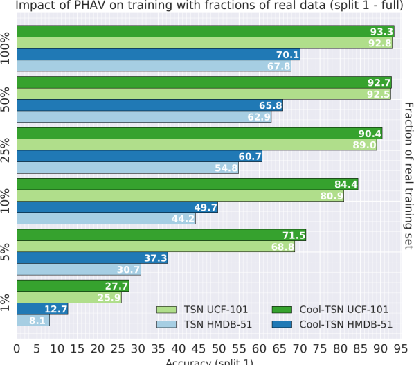
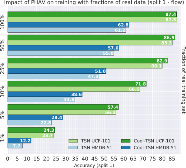
Figure 19: TSN and Cool-TSN results for different amounts of real-world training data, for each separate stream, and for each dataset.

7.3 Cool Temporal Segment Networks

In Table 6 we also report results of our Cool-TSN multi-task representation learning, (Section 6.2) which additionally uses PHAV to train UCF-101 and HMDB-51 models. We stop training after $3,000$ iterations for RGB streams and $20,000$ for flow streams, all other parameters as in (Wang et al., 2016b). Our results suggest that leveraging PHAV through either Cool-TSN or TSN-FT yields recognition improvements for all modalities in all datasets, with advantages in using Cool-TSN especially for the smaller HMDB-51. This provides quantitative experimental evidence supporting our claim that procedural generation of synthetic human action videos can indeed act as a strong prior (TSN-FT) and regularizer (Cool-TSN) when learning deep action recognition networks.

We further validate our hypothesis by investigating the impact of reducing the number of real world training videos (and iterations), with or without the use of PHAV. Our results reported in Table 7 and Figure 19 confirms that reducing training data from the target dataset impacts more severely TSN than Cool-TSN. HMDB displays the largest gaps. We partially attribute this to the smaller size of HMDB and also because some categories of PHAV overlap with some categories of HMDB. Our results show that it is possible to replace half of HMDB with procedural videos and still obtain comparable performance to using the full dataset (65.8 vs. 67.8). In a similar way, and although actions differ more, we show that reducing UCF-101 to a quarter of its original training set still yields a Cool-TSN model that rivals competing methods (Wang et al., 2016c; Simonyan and Zisserman, 2014; Wang et al., 2015). This shows that our procedural generative model of videos can indeed be used to augment different small real-world training sets and obtain better recognition accuracy at a lower cost in terms of manual labor.

Table 7: TSN and Cool-TSN with different fractions of real-world training data.

Fraction of real	UCF101	UCF101+PHAV	HMDB51	HMDB51+PHAV
-world samples	(TSN)	(Cool-TSN)	(TSN)	(Cool-TSN)
1%	25.9	27.7	8.1	12.7
5%	68.5	71.5	30.7	37.3
10%	80.9	84.4	44.2	49.7
25%	89.0	90.4	54.8	60.7
50%	92.5	92.7	62.9	65.8
100%	92.8	93.3	67.8	70.1

• Mean Accuracy (mAcc) in split 1 of each respective real-world dataset.

We also evaluate the impact of the failure cases described in Section 4. Using an earlier version of this dataset containing a similar amount of videos but an increased level of procedural noise, we retrained our models and compare them in Table 8. Our results show that, even though this kind of noise can result in small performance variations in individual streams, it has little effect when both streams are combined.

Table 8: Performance comparison considering an increased number of failure cases (noise).

Target	Noise	Spatial	Temporal	Full
UCF-101	20%	86.1	90.1	94.2
UCF-101	10%	86.3	89.9	94.2
HMDB-51	20%	52.4	64.1	69.5
HMDB-51	10%	53.0	63.9	69.5

• Average mean accuracy across all dataset splits.

Table 9: Comparison against the state of the art in action recognition.

			UCF-101	HMDB-51
	Method		%mAcc	%mAcc
One source	iDT+FV	Wang and Schmid (2013)	84.8	57.2
	iDT+StackFV	Peng et al. (2014)	-	66.8
	iDT+SFV+STP	Wang et al. (2016a)	86.0	60.1
	iDT+MIFS	Lan et al. (2015)	89.1	65.1
	VideoDarwin	Fernando et al. (2015)	-	63.7
Multiple sources	2S-CNN	Simonyan and Zisserman (2014)	88.0	59.4
	TDD	Wang et al. (2015)	90.3	63.2
	TDD+iDT	Wang et al. (2015)	91.5	65.9
	C3D+iDT	Tran et al. (2015)	90.4	-
	Actions$\sim$Trans	Wang et al. (2016c)	92.0	62.0
	2S-Fusion	Feichtenhofer et al. (2016)	93.5	69.2
	Hybrid-iDT	De Souza et al. (2016)	92.5	70.4
	3-TSN	Wang et al. (2016b)	94.0	68.5
	9-TSN	Wang et al. (2017)	94.9	-
	I3D	Carreira and Zisserman (2017)	97.9	80.2
	CMSN (C3D)	Zolfaghari et al. (2017)	91.1	69.7
	CMSN (TSN)	Zolfaghari et al. (2017)	94.1	-
	RADCD	Zhao et al. (2018)	95.9	-
	OFF	Sun et al. (2018)	96.0	74.2
	VGAN	Vondrick et al. (2016)	52.1	-
	Cool-TSN	This work	94.2	69.5

• Average Mean Accuracy (mAcc) across all dataset splits.

7.4 Comparison with the state of the art

In this section, we compare our model with the state of the art in action recognition (Table 9). We separate the current state of the art into works that use one or multiple sources of training data (such as by pre-training, multi-task learning or model transfer). We note that all works that use multiple sources can potentially benefit from PHAV without any modifications. Our results indicate that our methods are competitive with the state of the art, including methods that use much more manually labeled training data like the Sports-1M dataset (Karpathy et al., 2014). More importantly, PHAV does not require a specific model to be leveraged and thus can be combined with more recent models from the current and future state of the art. Our approach also leads to better performance than the current best generative video model VGAN (Vondrick et al., 2016) on UCF101, for the same amount of manually labeled target real-world videos. We note that while VGAN’s more general task is quite challenging and different from ours, Vondrick et al. (2016) has also explored VGAN as a way to learn unsupervised representations useful for action recognition, thus enabling our comparison.

8 Discussion

Our approach combines standard techniques from computer graphics (notably procedural generation) with deep learning for action recognition. This opens interesting new perspectives for video modeling and understanding, including action recognition models that can leverage algorithmic ground truth generation for optical flow, depth, semantic segmentation, or pose. In this section, we discuss some of these ideas, leaving them as indications for future work.

Integration with GANs.

Generative models like VGAN (Vondrick et al., 2016) can be combined with our approach by being used for dynamic background generation, domain adaptation of synthetic data, or real-to-synthetic style transfer, e.g., as Gatys et al. (2016). In addition, since our parametric model is able to leverage MoCap sequences, this opens the possibility of seeding our approach with synthetic sources of motion sequences, e.g., from works such as (Yan et al., 2018), while enforcing physical plausibility (thanks to our use of ragdoll physics and a physics engine) and generating pixel-perfect ground-truth for tasks such as semantic segmentation, instance segmentation, depth estimation, and optical flow.

Extension to complex activities.

Using ragdoll physics and a large enough library of atomic actions, it is possible to create complex actions by hierarchical composition. For instance, our “Car Hit” action is procedurally defined by composing atomic actions of a person (walking and/or doing other activities) with those of a car (entering in a collision with the person), followed by the person falling in a physically plausible fashion. However, while atomic actions have been validated as an effective decomposition for the recognition of potentially complex actions (Gaidon et al., 2013), we have not studied how this approach would scale with the complexity of the actions, notably due to the combinatorial nature of complex events.

Learning from a real world dataset.

While we initialize most of our parameters using uniform distributions, it is also possible to have them learned from real world datasets using attribute predictors, e.g., (Nian et al., 2017) or by adapting (Abdulnabi et al., 2015) to video. We note that $\bm{\theta_{D}}$ can be initialized by first training a classifier to distinguish between day phases in video (or images) then applying it to all clips (or frames, followed by pooling) of UCF-101 in order to retrieve the histogram of day phases in this dataset. We could then use the relative frequency of this histogram to initialize $\bm{\theta_{D}}$ We note that this technique could be used to initialize directly $\bm{\theta_{D}}$, $\bm{\theta_{W}}$, and $\bm{\theta_{C}}$. It could also be used to initialize $\bm{\theta_{E}}$ and $\bm{\theta_{H}}$ if those variables are further decomposed into more readily interpretable characteristics that could be easily annotated by crowdsourcing, e.g., “presence of grass”, “presence of water”, “filmed indoors”. Then, it becomes possible to learn classifiers for these attributes and establish a mapping between these and the different environments and cameras we use. It should also be possible to go further and learn attribute predictors for our virtual world as well, and embed attributes for virtual and real worlds in the same embedding space in order to learn this mapping automatically.

Including representative action classes.

In our experiments, we have found that certain classes benefit more from the extra virtual data available than others, e.g., “throw”. In the case of UCF-101, the top classes that improved the most were those that related the most with the virtual classes we included in our dataset, e.g., “fall floor” (“dive floor” in PHAV), “throw”, “jump”, “push”, and “shoot_ball”. This indicates that one of the crucial factors in improving the performance of classification models for target real-world datasets is indeed to include synthetic data for action classes also present in such datasets. Furthermore, one could also perform a ceteris paribus analysis in order to determine the impact of other parameters besides the action class (e.g., weather, presence of objects).

9 Conclusion

In this work, we have introduced a generative model for videos combining probabilistic graphical models and game engines, and have used it to instantiate PHAV, a large synthetic dataset for action recognition based on a procedural generative model of videos. Although our model does not learn video representations like VGAN, it can generate many diverse training videos thanks to its grounding in strong prior physical knowledge about scenes, objects, lighting, motions, and humans.

We provide quantitative evidence that our procedurally generated videos can be used as a simple complement to small training sets of manually labeled real-world videos. Importantly, we show that we do not need to generate training videos for particular target categories fixed a priori. Instead, surrogate categories defined procedurally enable efficient multi-task representation learning for potentially unrelated target actions that have few real-world training examples.

Appendix A Appendix

In this appendix, we include random frames (Figures 21, 22, 23, 24, and 25) for a subset of the action categories in PHAV, followed by a table of pixel colors (Table 10) used in our semantic segmentation ground-truth.

The frames below show the effect of different variables and motion variations being used (cf. Table 4). Each frame below is marked with a label indicating the value for different variables during the execution of the video, using the legend shown in Figure 20.

Figure 20: Legend for synthetic action video variations to be used in Figs. 21, 22, 23, 24, and 25.

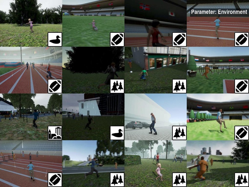
Figure 21: Changing environments. Top: kick ball, bottom: synthetic car hit.

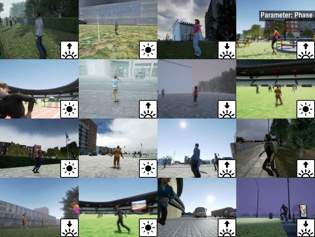
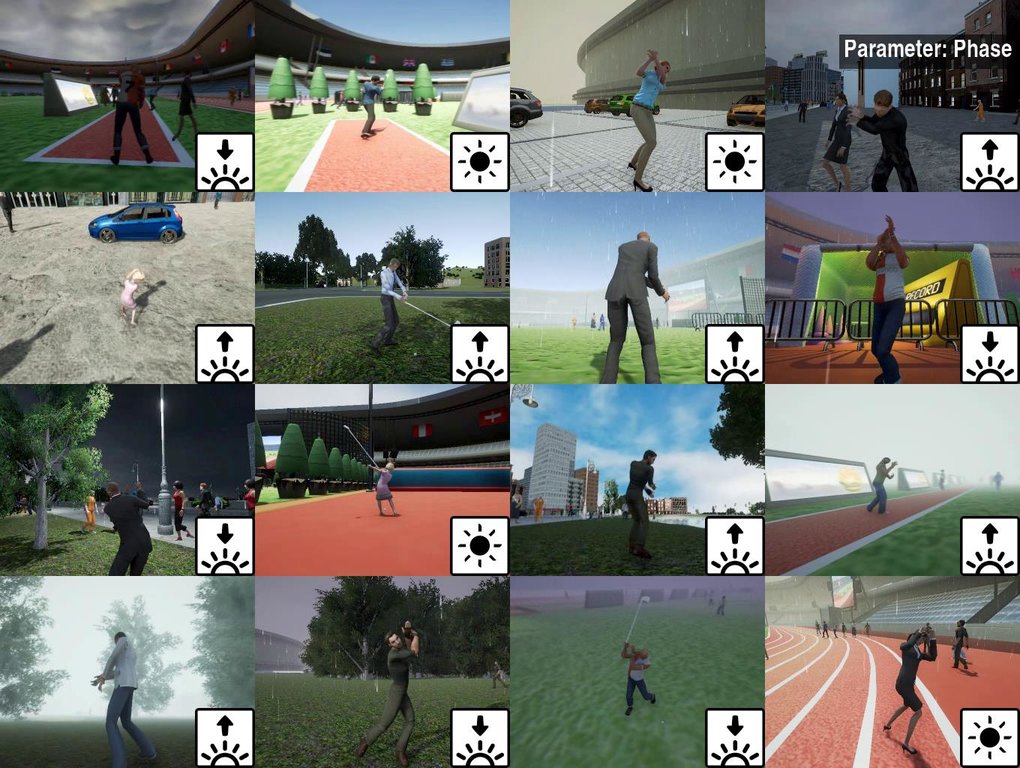
Figure 22: Changing phases of the day. Top: run, bottom: golf.

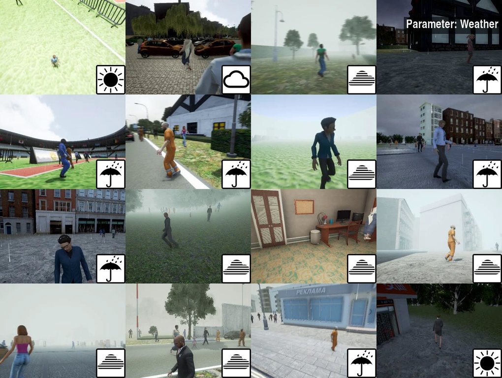
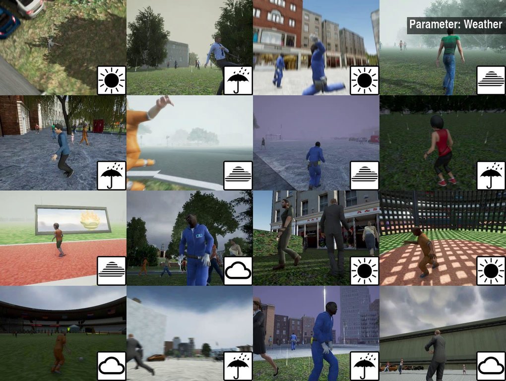
Figure 23: Changing weather. Top: walk, bottom: kick ball.

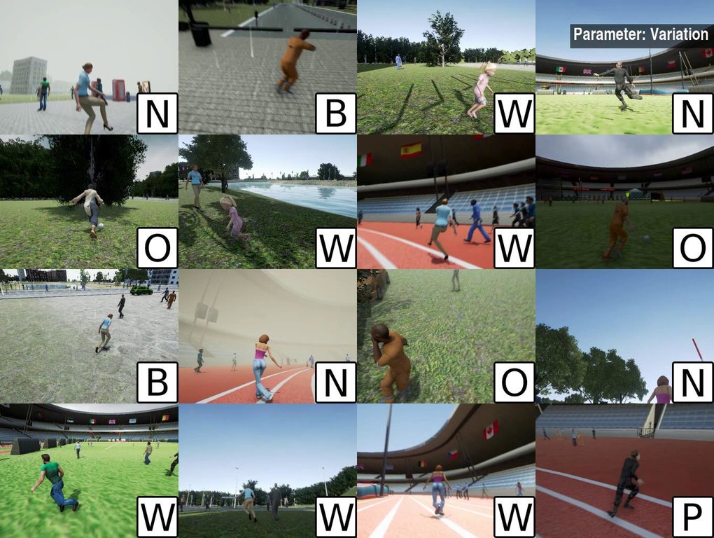
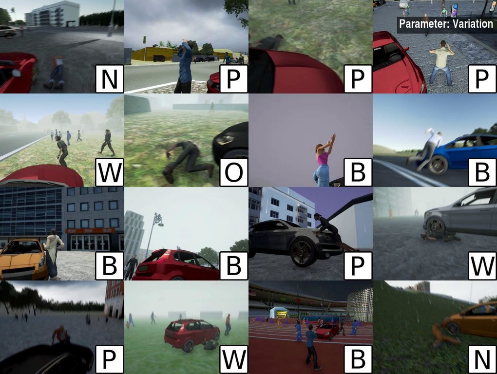
Figure 24: Changing motion variations. Top: kick ball, bottom: synthetic car hit.

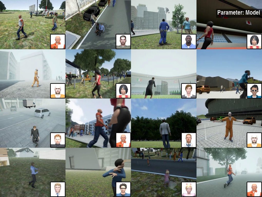
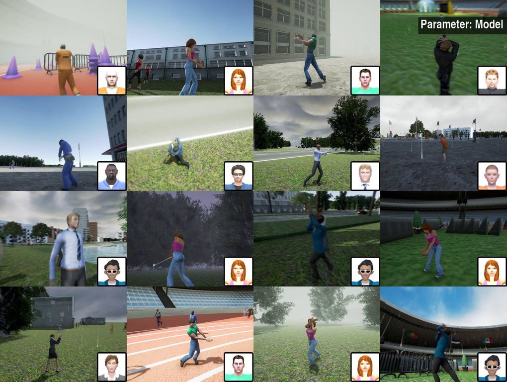
Figure 25: Changing human models. Top: walk, bottom: golf.

Table 10: Pixel-wise object-level classes in PHAV.

Group Pixel class R G B Virtual KITTI (Gaidon et al., 2016) CityScapes (Cordts et al., 2016) Road 100 60 100 Building 140 140 140 Pole 255 130 0 TrafficLight 200 200 0 TrafficSign 255 255 0 Vegetation 90 240 0 Terrain 210 0 200 Sky 90 200 255 Car 255 127 80 Truck 160 60 60 Bus 0 139 139 Misc 80 80 80 Tree 0 199 0 ADE20k (Zhou et al., 2017) Indoors Ceiling 240 230 140 Floor 0 191 255 Chair 72 61 139 Table 255 250 205 Bed 205 92 92 Lamp 160 82 45 Sofa 128 0 128 Window 0 128 0 Door 127 255 212 Stairs 219 112 147 Curtain 230 230 250 Fireplace 233 150 122 Shelf 153 50 204 Bench 245 222 179 Screen 218 165 32 Fridge 255 255 240 Interaction objects Ball 178 34 34 Baseball Bat 210 105 30 Gun 255 248 220 Golf Club 173 255 47 Hair Brush 224 255 255 PHAV-only Bow 95 158 160 Group Pixel class R G B Human Parts Head 220 20 60 RightUpperArm 255 255 26 RightLowerArm 255 215 0 RightHand 255 140 0 LeftUpperArm 60 179 113 LeftLowerArm 135 206 235 LeftHand 100 149 237 Chest 248 248 255 RightUpperLeg 102 51 153 RightLowerLeg 164 89 58 RightFoot 220 173 116 LeftUpperLeg 0 0 139 LeftLowerLeg 255 182 193 LeftFoot 255 239 213 Joints Neck 152 251 152 LeftShoulder 47 79 79 RightShoulder 85 107 47 LeftElbow 25 25 112 RightElbow 128 0 0 LeftWrist 0 255 255 RightWrist 238 130 238 LeftHip 147 112 219 RightHip 143 188 139 LeftKnee 102 0 102 RightKnee 69 33 84 LeftAnkle 50 205 50 RightAnkle 255 105 180 Pixel-wise object-level classes in PHAV. Some of the classes have been derived from semantic segmentation labels present in other datasets. These include: CityScapes (Cordts et al., 2016), mostly for outdoor object classes; Virtual KITTI (Gaidon et al., 2016), which contains a subset of the class labels in CityScapes; and ADE20k (Zhou et al., 2017), mostly for indoor object classes. The human body has been segmented in 14 parts and 13 joints, for a total of 27 segments. We note that our chosen separation can be combined to recover part separations used in PASCAL-Part (Chen et al., 2018) and J-HMDB (Jhuang et al., 2013) datasets.