Graph Spectral Embedding for Parsimonious
Transmission of Multivariate Time Series

Abstract

We propose a graph spectral representation of time series data that 1) is parsimoniously encoded to user-demanded resolution; 2) is unsupervised and performant in data-constrained scenarios; 3) captures event and event-transition structure within the time series; and 4) has near-linear computational complexity in both signal length and ambient dimension. This representation, which we call Laplacian Events Signal Segmentation (LESS), can be computed on time series of arbitrary dimension and originating from sensors of arbitrary type. Hence, time series originating from sensors of heterogeneous type can be compressed to levels demanded by constrained-communication environments, before being fused at a common center.

Temporal dynamics of the data is summarized without explicit partitioning or probabilistic modeling. As a proof-of-principle, we apply this technique on high dimensional wavelet coefficients computed from the Free Spoken Digit Dataset to generate a memory efficient representation that is interpretable. Due to its unsupervised and non-parametric nature, LESS representations remain performant in the digit classification task despite the absence of labels and limited data.

1 Introduction

The historical development of machine learning algorithms on time series data has followed a clear trend from initial simplicity to state-driven complexity. For instance, limitations in the Hidden Markov Model (see [27] for a survey) for modeling long range dependencies motivated the development of more complex but also more expressive neural networks, such as Recurrent Neural Networks [6] or Long Short-Term Memory model [15]. In this parametric learning framework, success in modeling temporal data has been largely dictated by the model’s ability to store appropriate latent states in memory, and to correctly transition between states according to underlying dynamics of the data.

Among gradient based models [10], interpreting these high dimensional latent states, as well as relating them to observations, remains a difficult area of research. Moreover, modeling dependencies within complex temporal data, such as speech audio [20] and financial pricing movements, requires a large number of observations, a requirement which often limits their application in real-life scenarios.

1.1 The LESS Algorithm

In this paper, we introduce an interpretable, unsupervised, non-parametric approach to time series segmentation called LESS: Laplacian Events Signal Segmentation. LESS is motivated by multi-scale geometric ideas, and its core computations are simple linear algebraic operations and convolution. The algorithm featurizes temporal data in a template-matching procedure using wavelets. The resulting wavelet coefficient representation is a trajectory in state-space. We interpret time steps of this representation as nodes of an underlying graph, whose graph structure is informed by events implicit in the original signal. A partitioning of this graph via its Laplacian embedding results in event segmentation of the signal.

LESS takes inspiration from the intuitive insight that naturally occurring temporal data have few meaningful event types, or motifs, and thus converting signals to event sequences has the potential to drastically reduce transmission and storage requirements. We aim to derive the simplest unsupervised technique that mirrors existing spectral clustering applications in image and graph data domains.

1.2 Outline

After surveying related work in Section 2, we give a detailed description of our proposed LESS technique in Section 3. Then Section 4 gives an empirical analysis of the robustness-to-noise of LESS, as well as a careful analysis of its computational complexity.

A first application of LESS is shown in Section 5. Using the Free Spoken Digits Dataset, we visualize the temporal dynamics of spoken audio with its segmentation into meaningful events, such as strong vs weak enunciations of ‘rho’ in ‘zero’, and show a clear contrast between representation trajectories in wavelet coefficient space belonging to different spoken digits. Furthermore, we show LESS has superior performance to Dynamic Time Warping [2] and to SAX [14] despite summarizing time series observations in far more parsimonious fashion.

Finally, although we do not pursue it formally in this paper, Section 6 outlines ways that LESS has strong potential to fit within upstream fusion pipelines of heterogeneous-modality time series. Hence, we argue that LESS will make a key contribution to unsupervised classification, visualization, and fusion tasks, especially in scenarios where training data is limited and/or communication between computational nodes is constrained.

2 Related Work

We briefly survey related work, and situate LESS within the context they define.

Connections to wavelet theory

Matching pursuit [5] projects signal data into its sparse approximation via a dictionary of wavelets. By computing the approximation error using this dictionary, the algorithm greedily selects a new wavelet that maximally reduces this error and adds it to the dictionary. Matching pursuit can encode a signal as its sparse approximation using few wavelets. Our algorithm similarly encodes an input signal via a wavelet dictionary. However, we further reduce this wavelet representation by computing its implicit motifs, summarizing it as a sequence of categorical values.

Similarly, wavelet scattering [16] [4] also utilizes a wavelet dictionary to derive sparse encodings of signals. In comparison to wavelet representations, scatter representations have the additional properties of being signal-translation invariant and capturing more complex frequency structure in the signal via its convolution network. We opt for wavelet scattering as the signal featurization procedure due to these additional properties. From the perspective of wavelet scattering, the LESS representation is in essence a temporal segmentation over the scatter coefficients.

Connections to graph theory

There have been numerous works (e.g, [9]) that process signals defined on the nodes of a graph. Tootooni et al [22] propose to monitor process drifts in multivariate time series data using spectral graph-based topological invariants. Like LESS, the proposed technique also considers multidimensional sensor signals and interprets an underlying state graph of the signal. By maintaining a window on an incoming stream of multidimensional data, vector time elements within the window form nodes of the graph. The authors observe that changes in the Fiedler number, a graph topological invariant computed from the graph’s Laplacian matrix, is informative towards process state. The empirical analysis demonstrates effective fault detection in process monitoring applications. LESS differs mainly by applying graph spectral techniques on wavelet-domain representations. In this way, complex frequency dynamics within the signal are accounted for in the state graph, and an event sequence representation of the signal in its entirety is generated by LESS, instead of a sequence of graph topological statistics emitted over the course of a sliding window.

Lacasa et al [11] propose the visibility algorithm, a process which converts time series into a visibility graph. Visibility graphs preserve the periodicity structure of the time series as graph regularity, while stochasticity in the time series are expressed as random graphs by the process. The visibility graph is invariant to translation and scaling of the time series, by which affine transformations of the time series lead to the same visibility graph. In comparison, our approach also generates translation invariant representations due to wavelet scattering. Periodicity within a time series is recognized as motifs by LESS, and as re-occuring tokens in the resulting event sequence representation.

Connections to time series modeling

Fused LASSO regression for multidimensional time series segmentation [18] combines breakpoint detection with computing breakpoint significance. After determining breakpoints implicit in the time series, their technique relies on clustering within each detected segment to estimate breakpoint significance. Similar to the proposed technique, LESS also seeks to address the multidimensional time series segmentation problem; although we segment according to a set of motifs implicitly determined by the time series, instead of identifying new segments for each local change in trend - this allows the desired number of motifs to be preset and easy identification of similar events, as they belong to the same motif.

Sprintz [3] is a time series compression technique leveraging a linear forecasting algorithm to be trained online for a data stream. By combining Delta Coding - a stateless, error-based forecast heuristic common in compression literature - with an autoregressive model of the form $x_{i}=ax_{i-1}+bx_{i-2}+\epsilon_{i}$, the authors are able to predict an upcoming delta as a rescaled version of the most recent delta, leading to a more expressive version of Delta Coding.

This forecasting component of Sprintz named ‘Fast Integer REgression’ (FIRE) is further supported by bit packing and Huffman coding to efficiently handle blocks of error values. In comparison, the objective of our paper is to find structure within time series data by unsupervised learning, then aggressively decrease data representation into a sequence of categoric tokens, corresponding to events. While our run-time scales worse by viewing the time series in its entirety, LESS representations have the flexibility to be of predetermined length, depending on user preference in the granularity of signal segmentation. Our representations also convey frequency-temporal structures within the time series.

SAX [14] creates a symbolic representation of the time series via Piecewise Aggregate Approximation (PAA). By dividing the time series data into equal frames, the PAA representation models the data with a linear combination of box basis functions. By binning the PAA coefficients according to the coefficient histogram, and setting the global frame size, lengths of SAX symbolic sequences are easily controlled. LESS controls the length of its output representation by $k$, the set of motifs hypothesized to be within the data. By decomposing the input signal via wavelet scattering, LESS featurization presents continuous signal structure in the frequency-temporal domain rather than discrete frames in the temporal domain. Moreover, the resulting wavelet coefficients are segmented by considering its relative location within the time series in wavelet coefficient space, rather than segmentation by binning according to a global coefficient histogram, as is the treatment of PAA coefficients by SAX.

3 The LESS Algorithm

The high-level steps (Figure 1 shows a flow diagram) in the LESS algorithm are as follows. First, wavelet scattering is applied to a raw time series $x$, resulting in a wavelet representation $z$. Then a weighted graph $G_{z}$ is computed from the wavelet representation, where the vertices of $G_{z}$ are $z[t],\quad t=1,\ldots,n$. The weighted edges of $G_{z}$ are computed from the self-similarity matrix of $z$ followed by a varying bandwidth kernel. Finally, spectral clustering is applied to extract an event sequence $e$, the final output of LESS. This section describes each of these technical steps in details. Further information on the parameters involved can be found in the Appendix.

Figure 1: A flow diagram for LESS.

3.1 Wavelet Representation

Wavelet scattering [4] creates a representation $\Phi x$ of a time series $x$ by composition of wavelet transforms. The main utility provided here is reducing uninformative variability in the signal - specifically translation in the temporal domain and noise components of the data. In the application of event segmentation, it is sufficient for wavelet scattering to capture the low frequency structure of $x$. These properties are explained in detail in the rest of this section. Throughout this paper, we refer to scatter representation $\Phi x$ as ‘the wavelet representation’, even if the terminology describes a broader family of wavelet-derived objects.

1. $\Phi x$ enables frequency selection
   

   The wavelet transform of $x$ is the set of coefficients computed by convolving $x$ with a wavelet dictionary of $J$ wavelets

   $$\{x*\Psi_{\lambda}(u)\}_{\lambda}$$

   where each wavelet is indexed by frequency $\lambda$. $\Psi_{\lambda}$ is convolved with the signal to emit coefficients corresponding to frequency $\lambda$. Wavelet scattering re-applies wavelet transform on the coefficients of this procedure with the same $q$ wavelets, under the condition that an identical wavelet cannot be applied to the coefficients more than once. For $p$ applications of wavelet transform, a set of convolution coefficients are generated, with set size ${q\choose p}$. We find that a small wavelet dictionary capturing low frequency components of $x$ is sufficient, leading to fast scatter computations and representations robust to instrumental noise (figure 7). In practice, $\Phi x$ is most effectively generated by 5 to 20 wavelets of lowest frequency, with $Q=2$.
   

2. $\Phi x$ is invariant to translations of $x$.
   

   That is, for a translation $c\in R$ and translated signal $x_{c}(u)=x(u-c)$, we have $\Phi x_{c}=\Phi x$. As the majority of wavelet techniques are covariant with translation, shifting $x$ in time alters the wavelet representation. As we seek to construct an underlying graph $G_{z}$ capturing the dynamics of $x$, translation invariance is an important property for leveraging spectral graph theory techniques. It’s relevance emerges when considering the instability of Laplacian eigenfunctions $L_{[v1,\ldots,v_{e}]}$ under a changing graph $G_{z}$. Despite being the same signal, shifts in the temporal domain of $x$ directly replaces vertices of $G_{z}$, dependent on magnitude of the shift $|c|$ relative to length of the data. See below for a detailed discussion.
   

3. $\Phi$ linearizes deformations in signal space.
   

   For a displacement field $\tau(u)$ (the deformation), $\Phi$ is Lipschitz continuous to deformations if there exists $C>0$ such that for all $\tau$ and $x$:

   $$||\Phi x_{\tau}-\Phi x||\leq C||x||\sup_{u}|\nabla\tau(u)|$$

   As an example, for a small deformation in the form of additive noise, $\Phi x-\Phi x_{\tau}$ is closely approximated by a bounded linear operator of $\tau$. Like translation invariance, $\Phi$’s linearization of deformations in signal space further reduces undesirable variability in the construction of $G_{z}$.

Figure 2: Top An example signal with it’s proposed segmentation $e$ displayed below. The signal begins and concludes with sinusoids of increasing oscillation, with an intermediate event. Bottom Normalized wavelet representation of the above signal. Only coefficients emitted by twelve wavelets of low frequency are considered. Notice the representation is invariant to non-stationarity and local trends, e.g. identical wavelet coefficients belonging to yellow events are generated for both a decreasing and an increasing trend in the signal. In addition, the entire signal follows an upward trend.

Every signal $x$ is mapped by wavelet scattering $\Phi$ to its wavelet representation $\Phi x=z$. In scatter coefficient space $Z$, undesirable variability in the space of signals $X$ is removed while the frequency-temporal structure of signals is preserved.

3.2 Wavelet Trajectory Graph $G_{z}$

Since $z$ may be iterated over by its temporal index $t$, $z$ is also a trajectory in wavelet coefficient space. A change in frequency structure of the signal, from here on recognized as an ‘event’, is reflected in $z$ by movement within wavelet coefficient space. Moreover, re-occuring events return the trajectory to the same region due to their similar frequency characteristics.

Figure 3: A visualization of spectral clustering in LESS. Figure 4 applies similar analysis on wavelet representations of real data. Left The wavelet coefficients of two wavelets is plotted as a trajectory in wavelet coefficient space. Center Dotted circles denote the range of adaptive kernels. Spectral clustering partitions wavelet coefficient space into non-convex regions according to population density. Right Solid lines denote strong edges of $G_{z}$, dashed lines denote weak edges.

Figure 4: To interpret the dynamics of wavelet coefficients, we project the wavelet coefficient space with time elements in $R^{40}$ to 2 principal components via PCA. Colored contours in both figures correspond to the same set of 7 motifs, as mapped by LESS ( red motif captures silence in the audio). To compute a common set of motifs among wavelet coefficients of the digit ‘one’ and ‘two’ classes, we concatenate the data. Differing density between digit classes cause different contour shapes of the same motif. Left 20 wavelet representations of the ‘one’ class is plotted in gray, with one example trajectory in black. Notice the bulk of observations do not exhibit black or purple events. Right 20 wavelet representations of the ‘two’ class, with one example in black. This class exhibits an extra event, colored in red-green. Wavelet coefficients of this class traverse toward the upper right direction in this projected space, differing from ‘one’.

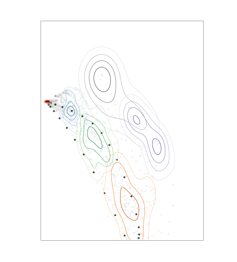
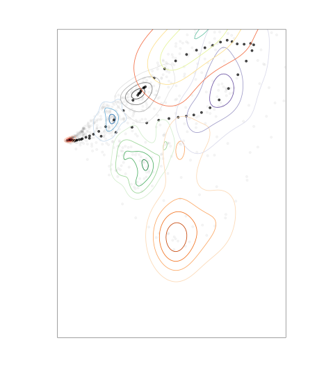
By segmenting $z$’s traversal to prevalent stationary and transitory patterns throughout time, we automate the identification of event motifs. See figure 3 for an illustration, and figure 4 for trajectory plots belonging to real data. The role of spectral clustering is identifying prevalent time series motifs. By segmentation of $z$’s dynamics according to motif durations, a sequence of events in $x$ is revealed.

The algorithm constructs an underlying graph $G_{z}$ of the wavelet representation $z$; the $n$ time elements of $z$ form the vertex set of $G_{z}$

$$V(G_{z})=\{z[t]\hphantom{12}|\quad t=1,\ldots,n\}$$

The weighted edges of $G_{z}$ are determined by the affinity matrix $W$ between time elements. The $z[t_{a}],z[t_{b}]$ pairwise affinity is

$$W(t_{a},t_{b})=\exp\left(-\frac{d(z[t_{a}],z[t_{b}])^{2}}{\sigma_{\omega}\sigma_{t_{a},t_{b}}}\right)$$

where $z[t]\in R^{p}$, $p$ the wavelet dictionary size. $d(\cdot,\cdot)$ is the euclidean distance, $\sigma_{\omega}$ a global scaling parameter. $\sigma_{t_{a},t_{b}}$ is the adaptive kernel size between time elements indexed at $t_{a}$ and $t_{b}$.

An adaptive kernel size, in contrast to a global kernel size, mitigates overly or sparsely sampled local neighborhoods. Following standard practice [25], we choose $\sigma_{a,b}$ as adaptive to local neighborhood distances. We compute the average distance between $z[t_{a}]$ and its $C$ nearest neighbors $N_{C}(z[t_{a}])$ to approximate the local sampling density, and denote this average neighborhood distance by $N_{t_{a}}$. The adaptive kernel is

$$\sigma_{t_{a},t_{b}}=\frac{N_{t_{a}}+N_{t_{b}}+d(z[t_{a}],z[t_{b}])}{3}$$

The interpretation of $z$ as a graph $G_{z}$ is quite literal. Observe that signal events inform the graph structure of $G_{z}$ - stationary trends in $x$ are easily captured as clique-like substructures in $G_{z}$, since stationary samples of the signal are all proximal in wavelet coefficient space. 2-state periodic behavior in $x$ may be reflected as a cycle connecting two cliques.

Figure 5: Affinity matrix $W$ displaying pairwise affinities between time elements of figure 2. The matrix center having high affinity is caused by the zero dominated middle interval of the wavelet representation. The interruption of this matrix block is caused by a light blue event around sample 9000 in the original signal. Diagonal lines of high affinity in the upper right quadrant (by symmetry of the similarity matrix, also the lower left quadrant) implies a recurrence of wavelet coefficient structure early in the signal with end of signal.

3.3 Event Identification

To exploit this insight on the connectivity and communal graph information, we leverage spectral clustering to automate the partitioning of $G_{z}$, where a subset of time elements $E\subset V(G_{z})$ corresponds to an event type in the data. At a high level, this is accomplished by embedding graph vertices by the eigenfunctions of the graph Laplacian $L$. Specifically, with adjacency matrix $A$ and degree matrix $D$ of $G_{z}$, we compute the normalized Laplacian

$$L=D^{-1/2}AD^{-1/2}$$

By applying eigendecomposition to $L$, we extract the eigenfunctions of the Laplacian. $L_{[v_{1},\ldots,v_{\Gamma}]}$, the Laplacian embedding of eigenfunctions corresponding to the smallest Laplacian eigenvalues, contains information regarding the stable cuts of $G_{z}$. See von Luxburg’s excellent survey [24] for a detailed treatment.

$L_{[v_{1},\ldots,v_{\Gamma}]}\in R^{|V(G_{z})|\times\Gamma}$ is a ‘tall’ matrix whose rows denote embedding coordinates for individual vertices. The eigenfunctions corresponding to larger eigenvalues yield more instable cuts, and therefore more noisy, vertex partitions. For most naturally occuring times series, the first three eigenfunctions of the graph Laplacian are sufficient. For the sake of clear notation, by $L_{v}$ we refer to the low rank embedding of $L_{[v_{1},v_{2},v_{3}]}$.

In $G_{z}$, each connected component is encoded by a Laplacian eigenvector within eigenspace 0 (in other words the geometric multiplicity of eigenvalue 0 matches number of connected components), where an eigenvector is an indicator vector with $1$ if the vertex belongs to that component. For Laplacian eigenvectors corresponding to non-zero eigenvalues, they partition connected components within $G_{z}$. The eigenvector of smallest non-zero eigenvalue, the Fiedler vector, lists a partition from the most stable cut of $G_{z}$ – a cut partitioning a connected component that acts most like a bottleneck of the component, i.e. in the context of the normalized Laplacian, a cut of maximal flow whose removal leads to two components of similar volume.

Finally, spectral clustering applies $k$-means clustering to $L_{v}$, assigning cluster memberships $\{E_{i}\}_{i}$ that partition $V(G_{z})$. $\cup_{i}E_{i}=V(G_{z})$. The number $k$ of cluster centroids, is a LESS parameter dictating the number of motifs to be considered while segmenting $x$. For larger $k$, higher time-resolution events may be observed, though overfitting in the form of short, spurious events is likely to occur.

By applying spectral clustering to the wavelet trajectory graph $G_{z}$, we partition the wavelet representation $z$, and by inversely mapping cluster assignments to the original temporal domain of the signal, LESS segments $x$ into a sequence of categoric tokens $e$, or event sequence of length $l$:

$$\text{LESS}(x)=e=\{e[1],\ldots,e[l]\}\quad e[i]\in\{1,\ldots,k\}$$

4 Properties and Computational Characteristics

4.1 Moving Average and Noise

This subsection describes two LESS properties: applications to signals with constant moving average and to noisy signals.

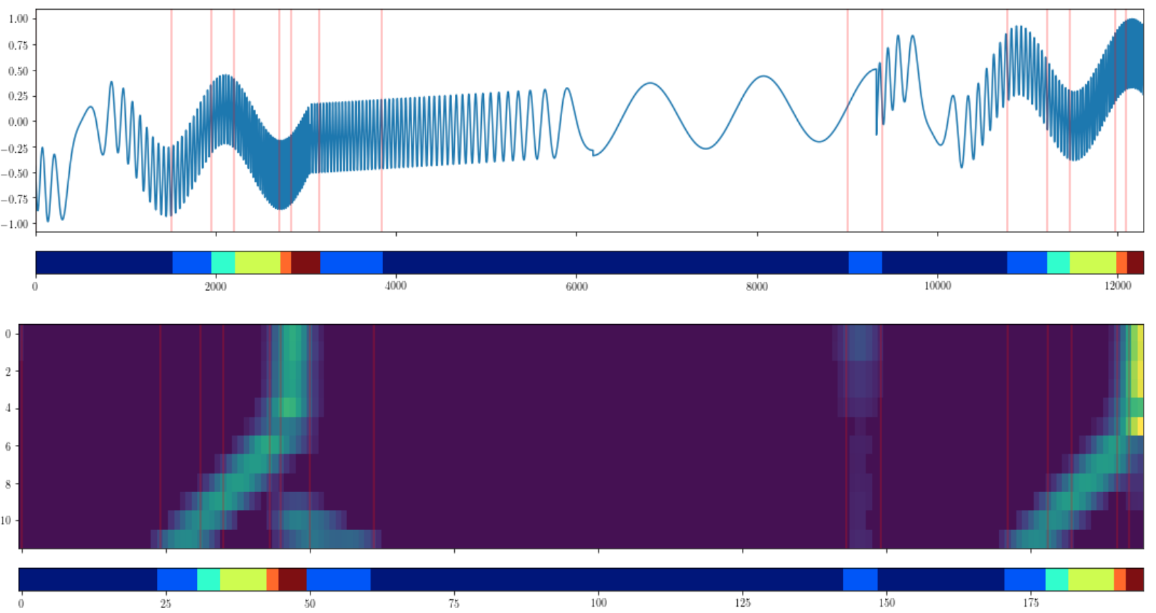
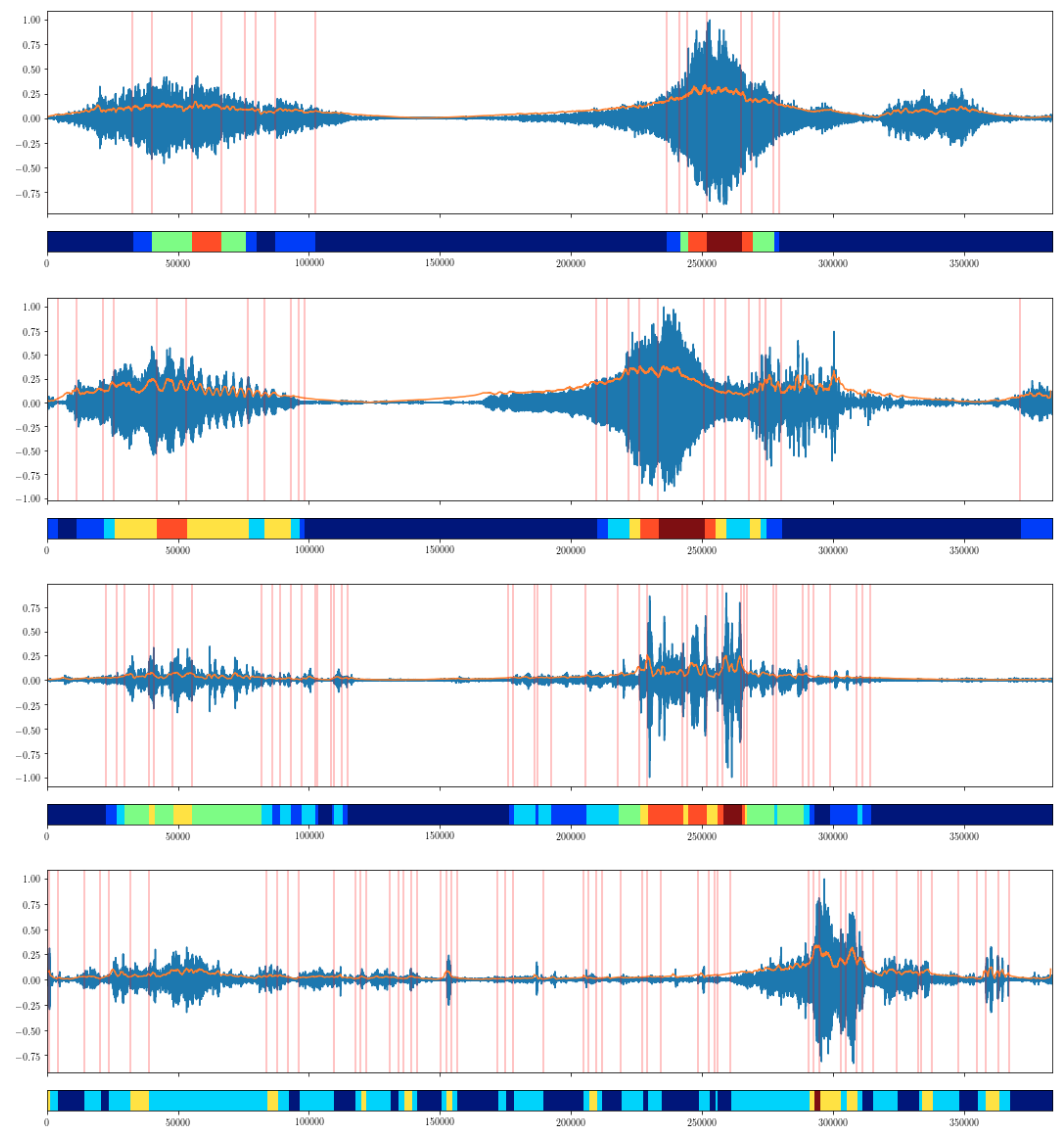
For signals with constant moving average through time, i.e. without trends, LESS event sequences tend to reflect local changes in Root Mean Square envelope and energy of the signal. To visualize this, LESS is applied to the recently-released ESCAPE dataset [28], a collection of live scenes where various vehicles are observed by sensors of different modalities. For illustration purposes here, we focus only on the audio modality and on four particular single-vehicle runs with vehicles of distinct types. In figure 6, four 1-minute audio recordings, belonging to single vehicles of different types, are concatenated then annotated by LESS. In the event sequences below each recording, common colors across observations denote events belonging to the same motif.

Figure 6: Four 1-minute audio recordings in the ESCAPE dataset, belonging to single vehicles of different types moving in the same trajectory. THE RMS envelope is shown in orange.

LESS representations remain robust in the presence of significant noise. By omitting wavelets corresponding to high frequency indices in wavelet scattering, the resulting wavelet representation $z$ does not account for high frequency structure in the original signal. Thus, while decreasing the number of necessary convolution operations, the algorithm regularizes the representation.

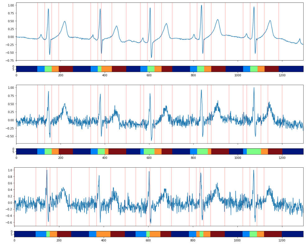
We illustrate this desirable property via an observation of the MIT BIH electrocardiogram data [17]. As heart muscles contract in a cyclical pattern, the cardiac cycle of P wave, QRS complex, ST segment and T wave is consistently identified by the event sequence of events light blue, green, orange, and brown respectively. In addition to the ECG signal, Gaussian noise of variance $\sigma=0.2$ and $\sigma=0.5$ was added. As seen in Figure 7, LESS has identified all noticeable patterns within the original signal accurately; moreover, it continues to output similar annotations under increasing noise.

Figure 7: An observation of the MIT BIH electrocardiogram data with its event sequence. Plots below has added Gaussian noise of variance $\sigma=0.2$ and $\sigma=0.5$. The cardiac cycle of P wave, QRS complex, ST segment and T wave is consistently identified by the event sequence of events light blue, green, orange, and brown respectively.

4.2 Computational Complexity and Scaling with Ambient Dimension

We analyze the computational load of LESS in this subsection. Note that LESS first applies wavelet scattering and then spectral clustering. In case of a multivariate signal, LESS computations scale linearly with size of the ambient dimension. Altogether, we claim that LESS has the following computational complexity

$$O\left(Dt\log t\right)+O(n^{3}),$$

where $D$ is the number of ambient dimensions, $t$ the length of the time series, and $n$ the number of time steps in wavelet representation. We argue below that $n\ll t$ in general practice, and thus the cubic term in the complexity analysis should not be that daunting.

To see this claim, we note (see [16]) that scattering computation on $1$-dimensional signals can be done in $O\left(\frac{1}{3}^{m}t\log t\right),$ with a signal of length $t$ and a scatter network of depth $m$. In practice, scatter networks of depth $m=2$ are optimal. Given a multivariate signal in $R^{D}$, we may naively apply the scatter computation $D$ times to generate coefficients for each dimension of the input, showing that the wavelet scattering of multivariate time series has complexity $O\left(Dt\log t\right).$ In practice, we note that modern numeric packages (e.g, kymatio [1]) for wavelet techniques leverage Graphic Processing Units (GPUs) to accelerate convolution operations.

The remainder of the computation concerns neither the number of ambient dimensions $D$ nor the length of input data $t$. During wavelet scattering, the extraction of wavelet coefficients is preceded by convolution with a low pass filter $\phi_{2^{J}}$, where the original length is sampled at intervals $2^{J}$, $J$ a scaling parameter set prior. Given a length $t$ signal, its wavelet representation has $n$ time steps: with increasing $J$, $n$ decreases exponentially relative to $t$. For most reasonable values of $J$, we have $n\ll t$.

Given a $D$ dimensional time series, there are $D$ applications of wavelet scattering, each application with the same wavelet dictionary of size $p$. What results is a dimension-wise concatenated wavelet representation of $Dp\times n$ coefficients. To compute the affinity matrix for spectral graph analysis, the $n$ vectors in $R^{Dp}$ are subtracted pairwise. Using vectorized subtraction, the distance matrix is computed in $O(n^{2})$. After transferring high dimensional coefficient information into connectivity relationships in the underlying graph $G_{z}$, the spectral clustering portion of the algorithm becomes agnostic to the ambient dimension of the input time series.

Lastly, spectral clustering’s computational bottleneck arises in acquiring a low rank approximation to the affinity matrix. Using the Nystrom method [13], there is an inherent two step orthogonalization procedure, where $O(n^{3})$ operations is incurred. In total, LESS operates with computational complexity $O\left(Dt\log t\right)+O(n^{3}),$ as claimed.

5 Application

This section outlines a first proof-of-principle application for LESS. We focus on distinguishing spoken digits from one another, using audio recordings, in an entirely unsupervised manner. That is, we use LESS to derive a distance between spoken audio observations, and then observe that clusters formed by this distance tend to correspond to digit type. The performance is especially encouraging when compared with two other common methods for deriving distances between time series data, Dynamic Time Warping and SAX.

The Free Spoken Digits Dataset(FSDD) consists of spoken digit recordings in wav files at 8kHz. FSDD contains 2,000 recordings from 4 speakers, each speaker saying digits 0 to 9 ten times per digit.

Figure 8: Levenshtein distances between event sequences. Contiguous slices of 10 rows/columns correspond to representations belonging to classes ‘zero’, ‘one’, and ‘three’ respectively. Lengths of event sequences range from four events (tokens) to eight.

Representations derived from the proposed technique remain informative towards classification tasks. To illustrate this, we compute within-class and between-class distances between event sequences. As example, given parameters $\theta$ and $k=3$ possible event types, $\{\alpha,\beta,\gamma\}$, LESS maps signal $x$ to an event sequence

$${[\alpha,\beta,\alpha,\gamma,\ldots,\beta]}$$

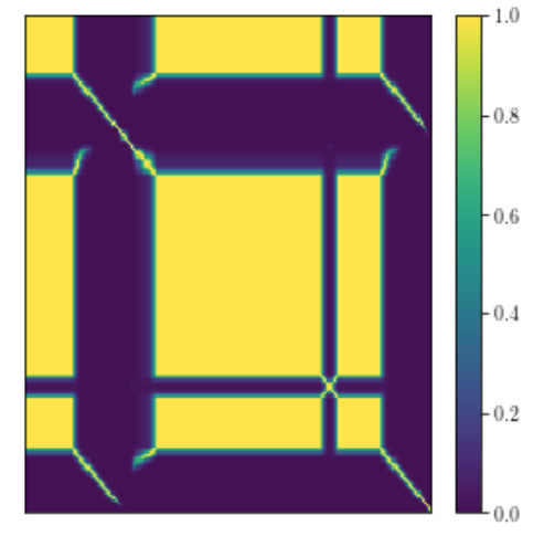
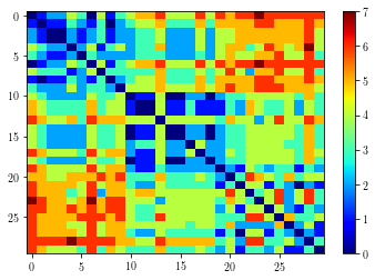
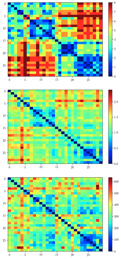
Such an event sequence contains categoric tokens corresponding to changes in the frequency structure of $x$, and consecutive tokens of the same motif are replaced with one in their place. The Levenshtein distance [12] is a standard method to compare any two token strings. Figure 8 shows the Levenshtein distance matrix computed between LESS representations of 30 short audio strings, 10 each of digit types ’0’, ’1’, and ’3.’ The rows of the matrix are ordered by digit type. For our choice of hyperparameters, the event sequence lengths range from four events (or tokens) to eight, ensuring transmission parsimony. Within each class, our technique generated event sequences that are, in expectation, 2 edits away. As seen in the block diagonal structure of the matrix, between class distances are higher.

We compare to two other methods of computing distances between signal snippets, Dynamic Time Warping (DTW, [2]) and SAX [14]. In brief, DTW produces an optimal match between the time indices of two time series observations that is robust to non-linear temporal distortions, in addition to temporal translation. Given a pair of signals $(x_{i},x_{j})$, the DTW distance refers to the minimal cost required to align time indices between $x_{i}$ and $x_{j}$, or equivalently the matching cost of their optimal match. Note that DTW can be computed on pairs of time series in any metric space; here we use it both in signal space $X$ and in wavelet coefficient space $Z$. SAX, on the other hand, creates a symbolic representation of the time series via Piecewise Aggregate Approximation (PAA). The output of SAX is very similar to that of LESS in form, namely a sequence of categorical tokens. Two such token sequences can then be compared using Levenshtein distance as above.

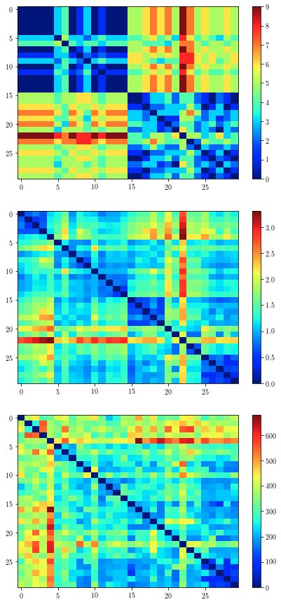
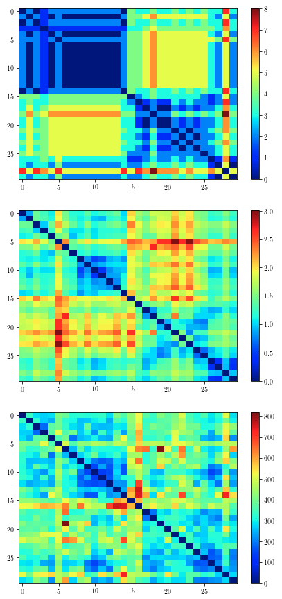
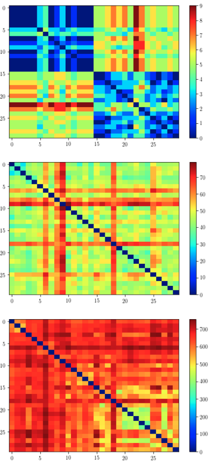
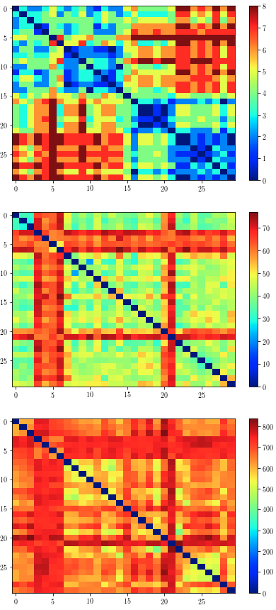
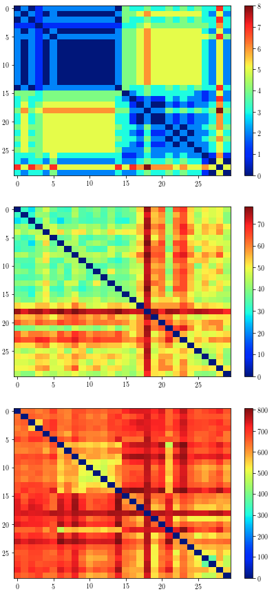
Figures 9 and 10 shows the results of the comparison experiments. Each column of each figure corresponds to a single experiment, where the task is to distinguish between $30$ spoken instances of two digit types. The top row in both figures uses the LESS-Levenshtein distance. The middle and bottom rows of Figure 9 use DTW computed on the scattering space time series and the raw time series, respectively. Qualitatively, the advantage of the LESS technique over the others at this task is clear. Furthermore, there are two other practical advantages: 1) in wallclock time, the approximal DTW algorithm, Fast DTW [19], took an order of magnitude of time longer than LESS while making $\binom{30}{2}$ comparisons; 2) the advantage of LESS over DTW in a communications-constrained environment should be clear: before DTW is computed on two signals arising from different sources, the entire signal must be transmitted, while LESS requires transmission of only the much shorter event sequence.

Figure 10 shows the same experiments in a comparison with SAX. A SAX parameter alphabet size is the number of token types available for labeling fixed width windows. We set alphabet size to 10 following the recommendation of SAX authors. We set representation lengths to be 100 (middle row) and 1000 (bottom row). For representation lengths of 1000, within-class structure begins to emerge in distance matrices. Again, the practical advantages of LESS in terms of computational speed and transmission in communications-constrained environments hold.

Figure 9: Each column corresponds to an experiment. Left column lists distances between spoken digits ‘one’ (row/col indices 0 to 14) and ‘six’ (row/col indices 15 to 29). Center column lists distances between ‘four’ and ‘seven’. Right column lists distances between ‘two’ and ‘five’. Top Levenshtein distance between LESS event sequences Center Distances approximated by Fast DTW when it is applied to wavelet representation time steps $z[t],\quad t=1,\ldots,n$ Bottom Signal distances approximated by Fast DTW. Notice in experiment 1, the observation at index 22 was considered far from all others in every distance.

Figure 10: Each column corresponds to an experiment. Left column lists distances between spoken digits ‘one’ (row/col indices 0 to 14) and ‘six’ (row/col indices 15 to 29). Center column lists distances between ‘four’ and ‘seven’. Right column lists distances between ‘two’ and ‘five’. Top Levenshtein distance between LESS event sequences, lengths varying from $4$ to $10$. Center SAX distance for alphabet size $10$ and representation length $100$. Bottom SAX distance for alphabet size $10$ and representation length $1000$.

6 Discussion

This paper presented LESS: Laplacian Events Signal Segmentation, a graph spectral representation of arbitrary-dimensional time series data. Despite its unsupervised nature, LESS is shown to be highly performant at a digit classification task, and especially so when judged in data and/or communication constrained environments. Further work will proceed along several fronts:

6.1 Memory Issues

Despite the nice computational complexity analysis above, the current implementation of LESS presents serious memory management issues on conventional hardware. An application of LESS requires the concatenation of multiple signals under consideration into one array, due to spectral clustering’s memory-less nature. This is impractical for large batches: 1) the eigendecomposition term in the complexity analysis $O(n^{3})$ dominates the computation and 2) $G_{z}$ may not be stored for the entire dataset $X$. Hence, on a desktop computer with conventional hardware, LESS may process 5-10 minutes of audio sampled at 48,000 Hz within 30 minutes.

Proximal and batch versions of spectral clustering [8] [26] offer solutions to alleviate this, both for maintaining adequate memory to store the graph $G_{z}$ and for tackling matrix computations on large batches of data. We will pursue these improvements in the near future.

6.2 Towards LESS as a Fusion Technique

The experiments above only display the benefits of LESS as a compression technique for tokenizing high-dimensional time series before transmission down a stingy channel. Beyond this paper, we are developing methods to use LESS within upstream fusion pipelines. The most immediate approach is to note that LESS involves the computation of a weighted graph based of a distance matrix (see the $G_{z}$ block in Figure 1). When faced with $n$ distinct time series ${\bf x}_{1},\ldots,{\bf x}_{n}$ of arbitrary dimensionality, one could simply run LESS up to this block, producing $n$ weighted graphs $G_{z_{1}},\ldots G_{z_{n}}$. Any number of distance-graph-based upstream fusion techniques (e.g, similarity network fusion [25], [23] or joint manifold learning [7], [21]) could then be used to produce a fused weighed graph $G_{f}$. The final step of LESS could then be applied to produce the fused event sequence. Experiments must be done to show that the resulting event sequence is indeed more informative, at tasks such as the ones outlined above, than stovepiped event sequences.

In a communication-constrained environment, the transmission of entire weighted graphs $G_{z_{i}}$ might be too expensive. Hence further work needs to be done on this front, either by: 1) pursuing sparse representations of the weighted graph, or; 2) creating an event-sequence-level fusion algorithm.

7 Appendix

This appendix gives more details on the parameters involved in LESS. All parameters are inherited from wavelet scattering and spectral clustering.

This paper implements wavelet scattering from the Kymatio package [1], and the parameter notations are adopted from Kymatio documentation. Scaling parameter $J\in Z$ dilates morlet wavelets by a factor of $2^{J}$. As a wavelet’s sinusoid component dilates, convolution with the signal leads to decorrelated scales. This reveals the frequency structure of the signal at a higher resolution, while decreasing temporal resolution. In practice $J$ in the range $[6,10]$ is suitable for most signal data, while short signals require $J<6$ due to the lack of adequate temporal support for wavelets. $Q$ is the number of first-order wavelets per octave. For most applications, incrementally exploring $q$ by multiples of $16$ seems efficient. In practice, selecting the $16$ wavelets indexed by lowest frequencies are sufficient.

$\sigma_{\omega}$, the spectral clustering parameter found in affinity matrix computations, controls the notion of global proximity. For increasing $\sigma_{\omega}$, kernel radii surrounding points expand, resulting in larger edges in $G_{z}$. For computing kernel sizes of a normalized pairwise-distance matrix, $\sigma_{\omega}\in[0.2,0.7]$ is optimal.

By examining the Laplacian eigenvectors $L_{[v_{1},\ldots,v_{\Gamma}]}$, $G_{z}$ vertices are encoded into the Laplacian embedding $R^{\Gamma}$. For all LESS experiments shown, only $\Gamma=3$ has been used; but membership information contained in eigenvectors of larger eigenvalues may prove beneficial.

Lastly $k$, the number of motifs, is the number of clusters in $k$-means clustering applied onto the embedding $L_{[v_{1},\ldots,v_{\Gamma}]}$. In simple signal data that rarely exhibit novel events, such as FSDD, $k=7$ is sufficient. On the other hand, to transform entire audio scenes, larger $k$ ($\geq 12$) is required.

The event sequence $e$ may be interpreted as annotation of the $n$ length wavelet representation $z$. While running various classification tasks, we find $e$ remains performant after discarding consecutive tokens of the same motif, and only note when the event type has changed.

References

- [1] Mathieu Andreux, Tomás Angles, Georgios Exarchakis, Roberto Leonarduzzi, Gaspar Rochette, Louis Thiry, John Zarka, Stéphane Mallat, Joakim Andén, Eugene Belilovsky, Joan Bruna, Vincent Lostanlen, Matthew J. Hirn, Edouard Oyallon, Sixhin Zhang, Carmine-Emanuele Cella, and Michael Eickenberg. Kymatio: Scattering transforms in python. CoRR, abs/1812.11214, 2018.
- [2] Donald J Berndt and James Clifford. Using dynamic time warping to find patterns in time series. In KDD workshop, volume 10, pages 359–370. Seattle, WA, 1994.
- [3] Davis Blalock, Samuel Madden, and John Guttag. Sprintz: Time series compression for the internet of things. Proc. ACM Interact. Mob. Wearable Ubiquitous Technol., 2(3):93:1–93:23, September 2018.
- [4] J. Bruna and S. Mallat. Invariant scattering convolution networks. IEEE Transactions on Pattern Analysis and Machine Intelligence, 35(8):1872–1886, Aug 2013.
- [5] T Tony Cai and Lie Wang. Orthogonal matching pursuit for sparse signal recovery with noise. Institute of Electrical and Electronics Engineers, 2011.
- [6] Zhengping Che, Sanjay Purushotham, Kyunghyun Cho, David Sontag, and Yan Liu. Recurrent neural networks for multivariate time series with missing values. Scientific reports, 8(1):6085, 2018.
- [7] Mark A. Davenport, Chinmay Hegde, Marco F. Duarte, and Richard G. Baraniuk. High dimensional data fusion via joint manifold learning. In AAAI Fall Symposium: Manifold Learning and Its Applications, 2010.
- [8] Yufei Han and Maurizio Filippone. Mini-batch spectral clustering. In 2017 International Joint Conference on Neural Networks (IJCNN), pages 3888–3895. IEEE, 2017.
- [9] Weiyu Huang, Thomas A. W. Bolton, John D. Medaglia, Danielle S. Bassett, Alejandro Ribeiro, and Dimitri Van De Ville. A graph signal processing view on functional brain imaging, 2017.
- [10] Brijnesh J. Jain. Generalized gradient learning on time series. Machine Learning, 100(2):587–608, Sep 2015.
- [11] Lucas Lacasa, Bartolo Luque, Fernando Ballesteros, Jordi Luque, and Juan Carlos Nuño. From time series to complex networks: The visibility graph. Proceedings of the National Academy of Sciences, 105(13):4972–4975, 2008.
- [12] Vladimir I Levenshtein. Binary codes capable of correcting deletions, insertions and reversals. In Soviet physics doklady, volume 10, page 707, 1966.
- [13] Mu Li, Xiao-Chen Lian, James T Kwok, and Bao-Liang Lu. Time and space efficient spectral clustering via column sampling. In CVPR 2011, pages 2297–2304. IEEE, 2011.
- [14] Jessica Lin, Eamonn Keogh, Li Wei, and Stefano Lonardi. Experiencing sax: a novel symbolic representation of time series. Data Mining and Knowledge Discovery, 15(2):107–144, Oct 2007.
- [15] Zachary C Lipton, David C Kale, Charles Elkan, and Randall Wetzel. Learning to diagnose with lstm recurrent neural networks. arXiv preprint arXiv:1511.03677, 2015.
- [16] Stephane Mallat. Group invariant scattering. Communications on Pure and Applied Mathematics, 65(10):1331–1398.
- [17] R.G. Mark, P.S. Schluter, G.B. Moody, P.H. Devlin, and D. Chernoff. An annotated ecg database for evaluating arrythmia detectors. IEEE Transactions on Biomedical Engineering, 29, 1982.
- [18] Nooshin Omranian, Bernd Mueller-Roeber, and Zoran Nikoloski. Segmention of biological multivariate time-series data. Scientific Reports, 2015.
- [19] Stan Salvador and Philip Chan. Toward accurate dynamic time warping in linear time and space. Intelligent Data Analysis, 11(5):561–580, 2007.
- [20] M. E. Sargin, Y. Yemez, E. Erzin, and A. M. Tekalp. Audiovisual synchronization and fusion using canonical correlation analysis. IEEE Transactions on Multimedia, 9(7):1396–1403, Nov 2007.
- [21] Dan Shen, Erik Blasch, Peter Zulch, Marcello Distasio, Ruixin Niu, Jingyang Lu, Zhonghai Wang, and Genshe Chen. A joint manifold leaning-based framework for heterogeneous upstream data fusion. Journal of Algorithms & Computational Technology, 12(4):311–332, 2018.
- [22] M. S. Tootooni, P. K. Rao, C. Chou, and Z. J. Kong. A spectral graph theoretic approach for monitoring multivariate time series data from complex dynamical processes. IEEE Transactions on Automation Science and Engineering, 15(1):127–144, Jan 2018.
- [23] Christopher J. Tralie, Paul Bendich, and John Harer. Multi-scale geometric summaries for heterogeneous sensor fusion. In Proc. 2019 IEEE Aerospace Conference.
- [24] Ulrike Von Luxburg. A tutorial on spectral clustering. Statistics and computing, 17(4):395–416, 2007.
- [25] Bo Wang, Aziz M Mezlini, Feyyaz Demir, Marc Fiume, Zhuowen Tu, Michael Brudno, Benjamin Haibe-Kains, and Anna Goldenberg. Similarity network fusion for aggregating data types on a genomic scale. Nature methods, 11(3):333, 2014.
- [26] Donghui Yan, Ling Huang, and Michael I Jordan. Fast approximate spectral clustering. In Proceedings of the 15th ACM SIGKDD international conference on Knowledge discovery and data mining, pages 907–916. ACM, 2009.
- [27] Walter Zucchini, Iain L MacDonald, and Roland Langrock. Hidden Markov models for time series: an introduction using R. Chapman and Hall/CRC, 2017.
- [28] Peter Zulch, Marcello DiStasio, Todd Cushman, Brian Wilson, Ben Hart, and Erik Blasch. Escape data collection for multi-modal data fusion research. In Proceedings of the 2019 IEEE Aerospace Conference.