Black-box Optimizer with Implicit Natural Gradient

Yueming Lyu
Australian Artificial Intelligence Institute
University of Technology Sydney
yueminglyu@gmail.com
&Ivor Tsang
Australian Artificial Intelligence Institute
University of Technology Sydney
Ivor.Tsang@uts.edu.au
Abstract

Black-box optimization is primarily important for many compute-intensive applications, including reinforcement learning (RL), robot control, etc. This paper presents a novel theoretical framework for black-box optimization, in which our method performs stochastic update with implicit natural gradient of an exponential-family distribution. Theoretically, we prove the convergence rate of our framework with full matrix update for convex functions. Our theoretical results also hold for continuous non-differentiable black-box functions. Our methods are very simple and contain less hyper-parameters than CMA-ESย [13]. Empirically, our method with full matrix update achieves a competitive performance compared with one of the state-of-the-art method CMA-ES on benchmark test problems. Moreover, our methods can achieve high optimization precision on some challenging test functions (e.g., l1subscript๐‘™1l_{1}-norm ellipsoid test problem and Levy test problem), while methods with explicit natural gradient, i.e., IGOย [23] with full matrix update can not. This shows the efficiency of our methods.

1 Introduction

Given a proper function fโ€‹(๐’™):โ„dโ†’โ„:๐‘“๐’™โ†’superscriptโ„๐‘‘โ„f({\boldsymbol{x}}):\mathbb{R}^{d}\rightarrow\mathbb{R} such that fโ€‹(๐’™)>โˆ’โˆž๐‘“๐’™f({\boldsymbol{x}})>-\infty, we aim at minimizing fโ€‹(๐’™)๐‘“๐’™f({\boldsymbol{x}}) by using function queries only, which is known as black-box optimization. It has a wide range of applications, such as automatic hyper-parameters tuning in machine learning and computer vision problems [27], adjusting parameters for robot control and reinforcement learningย [9, 18, 7], black-box architecture search in engineering designย [30] and drug discoveryย [21].

Several kinds of approaches have been widely studied for black-box optimization, including Bayesian optimization (BO) methodsย [29, 8, 20], evolution strategies (ES)ย [5, 13] and genetic algorithms (GA)ย [28]. Among them, Bayesian optimization methods are good at dealing with low-dimensional expensive black-box optimization, while ES methods are better for relatively high-dimensional problems with cheaper evaluations compared with BO methods. ES-type algorithms can well support parallel evaluation, and have drawn more and more attention because of its success in reinforcement learning problemsย [11, 26, 17], recently.

CMA-ESย [13] is one of state-of-the-art ES methods with many successful applications. It uses second-order information to search candidate solutions by updating the mean and covariance matrix of the likelihood of candidate distributions. Despite its successful performance, the update rule combines several sophisticated components, which is not well understood. Wierstra et al. show that directly applying standard reinforce gradient descent is very sensitive to variance in high precision search for black-box optimizationย [31]. Thus, they propose Natural evolution strategies (NES)ย [31] to estimate the natural gradient for black-box optimization. However, they use the Monte Carlo sampling to approximate the Fisher information matrix (FIM), which incurs additional error and computation cost unavoidably. Along this line, [1] show the connection between the rank-ฮผ๐œ‡\mu update of CMA-ES and NESย [31]. [23] further show that several ES methods can be included in an unified framework. Despite these theoretical attempts, the practical performance of these methods is still inferior to CMA-ES. Moreover, these works do not provide any convergence rate analysis, which is the key insight to expedite black-box optimizations.

Another line of research for ES-type algorithms is to reduce the variance of gradient estimators. Choromanski et al.ย [11] proposed to employ Quasi Monte Carlo (QMC) sampling to achieve more accurate gradient estimates. Recently, they further proposed to construct gradient estimators based on active subspace techniquesย [10]. Although these works can reduce sample complexity, how does the variance of these estimators influence the convergence rate remains unclear.

To take advantage of second-order information for the acceleration of black-box optimizations, we propose a novel theoretical framework: stochastic Implicit Natural Gradient Optimization (INGO) algorithms, from the perspective of information geometry. Raskutti et al.ย [24] give a method to compute the Fisher information matrix implicitly using exact gradients, which is impossible for black-box optimization; while our methods and analysis focus on black-box optimization. To the best of our knowledge, we are the first to design stochastic implicit natural gradient algorithms w.r.t natural parameters for black-box optimization. Our methods take a stochastic black-box estimate instead of the exact gradient to update. Theoretically, this update is equivalent to a stochastic natural gradient step w.r.t. natural parameters of an exponential-family distribution. Our contributions are summarized as follows:

  • โ€ข

    We propose a novel stochastic implicit natural gradient descent framework for black-box optimization (INGO). To the best of our knowledge, we are the first to design stochastic implicit natural gradient algorithms w.r.t natural parameters for black-box optimization. We propose efficient algorithms for both continuous and discrete black-box optimization. Our methods construct stochastic black-box update without computing the FIM. Our method can adaptively control the stochastic update by taking advantage of the second-order information, which is able to accelerate convergence and is primarily important for ill-conditioned problems. Moreover, our methods have fewer hyperparameters and are much simpler than CMA-ES.

  • โ€ข

    Theoretically, we prove the convergence rate of our continuous optimization methods for convex functions. Our theoretical results also hold for non-differentiable convex black-box functions. This is distinct from most literature works that need Lipschitz continuous gradients (L๐ฟL-smooth) assumption. Our theoretical results can include many interesting problems with non-smooth structures. We also show that reducing variance of the black-box gradient estimators by orthogonal sampling can lead to a small regret bound.

  • โ€ข

    Empirically, our continuous optimization method achieves a competitive performances compared with the state-of-the-art method CMA-ES on benchmark problems. We find that our method with full matrix update can obtain higher optimization precision compared with IGOย [23] on some challenging problems. We further show the effectiveness of our methods on RL control problems. Moreover, our discrete optimization algorithm outperforms GA method.

2 Notation and Symbols

Denote โˆฅโ‹…โˆฅ2\|\cdot\|_{2} and โˆฅโ‹…โˆฅF\|\cdot\|_{F} as the spectral norm and Frobenius norm for matrices, respectively. Define โ€–Yโ€–tโ€‹r:=โˆ‘i|ฮปi|assignsubscriptnorm๐‘Œ๐‘ก๐‘Ÿsubscript๐‘–subscript๐œ†๐‘–\|Y\|_{tr}:=\sum_{i}{|\lambda_{i}|}, where ฮปisubscript๐œ†๐‘–\lambda_{i} denotes the itโ€‹hsuperscript๐‘–๐‘กโ„Ži^{th} eigenvalue of matrix Y๐‘ŒY. Notation โˆฅโ‹…โˆฅ2\|\cdot\|_{2} will also denote l2subscript๐‘™2l_{2}-norm for vectors. Symbol โŸจโ‹…,โ‹…โŸฉโ‹…โ‹…\left<\cdot,\cdot\right> denotes inner product under l2subscript๐‘™2l_{2}-norm for vectors and inner product under Frobenius norm for matrices. Define โ€–๐’™โ€–C:=โŸจ๐’™,Cโ€‹๐’™โŸฉassignsubscriptnorm๐’™๐ถ๐’™๐ถ๐’™\|\boldsymbol{x}\|_{C}:=\sqrt{\left<\boldsymbol{x},C\boldsymbol{x}\right>}. Denote ๐’ฎ+superscript๐’ฎ\mathcal{S}^{+} and ๐’ฎ++superscript๐’ฎabsent\mathcal{S}^{++} as the set of positive semi-definite matrices and the set of positive definite matrices, respectively. Denote ฮฃ12superscriptฮฃ12\Sigma^{\frac{1}{2}} as the symmetric positive semi-definite matrix such that ฮฃ=ฮฃ12โ€‹ฮฃ12ฮฃsuperscriptฮฃ12superscriptฮฃ12\Sigma=\Sigma^{\frac{1}{2}}\Sigma^{\frac{1}{2}} for ฮฃโˆˆ๐’ฎ+ฮฃsuperscript๐’ฎ\Sigma\in\mathcal{S}^{+}.

3 Implicit Natural Gradient Optimization

3.1 Optimization with Exponential-family Sampling

We aim at minimizing a proper function fโ€‹(๐’™)๐‘“๐’™f({\boldsymbol{x}}), ๐’™โˆˆ๐’ณ๐’™๐’ณ{\boldsymbol{x}}\in\mathcal{X} with only function queries, which is known as black-box optimization. Due to the lack of gradient information for black-box optimization, we here present an exponential-family sampling trick to relax any black-box optimization problem. Specifically, the objective is relaxed as the expectation of fโ€‹(๐’™)๐‘“๐’™f({\boldsymbol{x}}) under a parametric distribution pโ€‹(๐’™;ฮท)๐‘๐’™๐œ‚p({\boldsymbol{x}};\eta) with parameter ฮท๐œ‚\eta, i.e., Jโ€‹(๐œผ):=๐”ผpโ€‹(๐’™;๐œผ)โ€‹[fโ€‹(๐’™)]assign๐ฝ๐œผsubscript๐”ผ๐‘๐’™๐œผdelimited-[]๐‘“๐’™J({\boldsymbol{\eta}}):=\mathbb{E}_{p({\boldsymbol{x}};{\boldsymbol{\eta}})}[f({\boldsymbol{x}})]ย [31]. The optimal parameter ๐œผ๐œผ{\boldsymbol{\eta}} is found by minimizing Jโ€‹(๐œผ)๐ฝ๐œผJ({\boldsymbol{\eta}}) as min๐œผโก{๐”ผpโ€‹(๐’™;๐œผ)โ€‹[fโ€‹(๐’™)]}subscript๐œผsubscript๐”ผ๐‘๐’™๐œผdelimited-[]๐‘“๐’™\min_{{\boldsymbol{\eta}}}\left\{\mathbb{E}_{p({\boldsymbol{x}};{\boldsymbol{\eta}})}[f({\boldsymbol{x}})]\right\} This relaxed problem is minimized when the probability mass is all assigned on the minimum of fโ€‹(๐’™)๐‘“๐’™f({\boldsymbol{x}}). The distribution p๐‘p is the sampling distribution for black-box function queries. Note, p๐‘p can be either continuous or discrete.

In this work, we assume that the distribution pโ€‹(๐’™;๐œผ)๐‘๐’™๐œผp({\boldsymbol{x}};{\boldsymbol{\eta}}) is an exponential-family distribution:

pโ€‹(๐’™;๐œผ)=hโ€‹(๐’™)โ€‹expโก{โŸจฯ•โ€‹(๐’™),๐œผโŸฉโˆ’Aโ€‹(๐œผ)},๐‘๐’™๐œผโ„Ž๐’™italic-ฯ•๐’™๐œผ๐ด๐œผ\displaystyle p({\boldsymbol{x}};{\boldsymbol{\eta}})=h({\boldsymbol{x}})\exp{\{\left<\phi({\boldsymbol{x}}),{\boldsymbol{\eta}}\right>-A({\boldsymbol{\eta}})\}}, (1)

where ๐œผ๐œผ{\boldsymbol{\eta}} and ฯ•โ€‹(๐’™)italic-ฯ•๐’™\phi({\boldsymbol{x}}) are the natural parameter and sufficient statistic, respectively. And Aโ€‹(ฮท)๐ด๐œ‚A(\eta) is the log partition function defined as A(ฮท)=logโˆซexp{โŸจฯ•(๐’™),๐œผโŸฉh(๐’™)d๐’™A(\eta)=\log\int\exp{\{\left<\phi({\boldsymbol{x}}),{\boldsymbol{\eta}}\right>}h({\boldsymbol{x}}){d\boldsymbol{x}}.

It is named as minimal exponential-family distribution when there is a one-to-one mapping between the mean parameter ๐’Ž:=๐”ผpโ€‹[ฯ•โ€‹(๐’™)]assign๐’Žsubscript๐”ผ๐‘delimited-[]italic-ฯ•๐’™{\boldsymbol{m}}:=\mathbb{E}_{p}[\phi({\boldsymbol{x}})] and natural parameter ๐œผ๐œผ{\boldsymbol{\eta}}. This one-to-one mapping ensures that we can reparameterize Jโ€‹(๐œผ)๐ฝ๐œผJ({\boldsymbol{\eta}}) as J~โ€‹(๐’Ž)=Jโ€‹(๐œผ)~๐ฝ๐’Ž๐ฝ๐œผ\tilde{J}({\boldsymbol{m}})=J({\boldsymbol{\eta}})ย [3, 14]. J~~๐ฝ\tilde{J} is w.r.t parameter ๐’Ž๐’Ž\boldsymbol{m}, while J๐ฝJ is w.r.t parameterย ๐œผ๐œผ\boldsymbol{\eta}.

To minimize the objective J~โ€‹(๐’Ž)~๐ฝ๐’Ž\tilde{J}({\boldsymbol{m}}), we desire the updated distribution lying in a trust region of the previous distribution at each step. Formally, we update the mean parameters by solving the following optimization problem.

๐’Žt+1=argโกmin๐’ŽโกโŸจ๐’Ž,โˆ‡๐’ŽJ~โ€‹(๐’Žt)โŸฉ+1ฮฒtโ€‹KLโ€‹(pmโˆฅpmt),subscript๐’Ž๐‘ก1subscript๐’Ž๐’Žsubscriptโˆ‡๐’Ž~๐ฝsubscript๐’Ž๐‘ก1subscript๐›ฝ๐‘กKLconditionalsubscript๐‘๐‘šsubscript๐‘subscript๐‘š๐‘ก\displaystyle{\boldsymbol{m}}_{t+1}\!\!=\!\!\arg\min_{{\boldsymbol{m}}}\!\left<{\boldsymbol{m}}\!,\!\nabla_{\boldsymbol{m}}\tilde{J}({\boldsymbol{m}_{t}})\!\right>\!+\!\frac{1}{\beta_{t}}\text{KL}\left(p_{m}\|p_{m_{t}}\right), (2)

where โˆ‡๐’ŽJ~โ€‹(๐’Žt)subscriptโˆ‡๐’Ž~๐ฝsubscript๐’Ž๐‘ก\nabla_{\boldsymbol{m}}\tilde{J}({\boldsymbol{m}}_{t}) denotes the gradient at ๐’Ž=๐’Žt๐’Žsubscript๐’Ž๐‘ก{\boldsymbol{m}}={\boldsymbol{m}}_{t}.

The KL-divergence term measures how close the updated distribution and the previous distribution. For an exponential-family distribution, the KL-divergence term in (2) is equal to Bregman divergence between ๐’Ž๐’Ž{\boldsymbol{m}} and ๐’Žtsubscript๐’Ž๐‘ก{\boldsymbol{m}}_{t}ย [4]:

KLโ€‹(pmโˆฅpmt)=Aโˆ—โ€‹(๐’Ž)โˆ’Aโˆ—โ€‹(๐’Žt)โˆ’โŸจ๐’Žโˆ’๐’Žt,โˆ‡๐’ŽAโˆ—โ€‹(๐’Žt)โŸฉ,KLconditionalsubscript๐‘๐‘šsubscript๐‘subscript๐‘š๐‘กsuperscript๐ด๐’Žsuperscript๐ดsubscript๐’Ž๐‘ก๐’Žsubscript๐’Ž๐‘กsubscriptโˆ‡๐’Žsuperscript๐ดsubscript๐’Ž๐‘ก\text{KL}\left(p_{m}\|p_{m_{t}}\right)\!=\!A^{*}({\boldsymbol{m}})\!-\!A^{*}({\boldsymbol{m}}_{t})\!-\!\left<{\boldsymbol{m}}\!-\!{\boldsymbol{m}}_{t},\nabla_{\boldsymbol{m}}A^{*}({\boldsymbol{m}}_{t})\right>, (3)

where Aโˆ—โ€‹(๐’Ž)superscript๐ด๐’ŽA^{*}({\boldsymbol{m}}) is the convex conjugate of Aโ€‹(๐œผ)๐ด๐œผA({\boldsymbol{\eta}}). Thus, the problem (2) is a convex optimization problem, and it has a closed-form solution.

3.2 Implicit Natural Gradient

Intractability of Natural Gradient for Black-box Optimization: Natural gradientย [2] can capture information geometry structure during optimization, which enables us to take advantage of the second-order information to accelerate convergence. Direct computation of natural gradient needs the inverse of Fisher information matrix (FIM), which needs to estimate the FIM. The method in [24] provides an alternative way to compute natural gradient without computation of FIM. However, it relies on the exact gradient, which is impossible for black-box optimization.

Hereafter, we propose a novel stochastic implicit natural gradient algorithms for black-box optimization of continuous and discrete variables in Sectionย 4 and Sectionย A (in the supplement), respectively. We first show how to compute the implicit natural gradient. In problem Eq.(2), we take the derivative w.r.t ๐’Ž๐’Ž{\boldsymbol{m}}, and set it to zero, also note that โˆ‡๐’ŽAโˆ—โ€‹(๐’Ž)=๐œผsubscriptโˆ‡๐’Žsuperscript๐ด๐’Ž๐œผ\nabla_{\boldsymbol{m}}A^{*}({\boldsymbol{m}})={\boldsymbol{\eta}}ย [24], we can obtain that

๐œผt+1=๐œผtโˆ’ฮฒtโ€‹โˆ‡๐’ŽJ~โ€‹(๐’Žt)subscript๐œผ๐‘ก1subscript๐œผ๐‘กsubscript๐›ฝ๐‘กsubscriptโˆ‡๐’Ž~๐ฝsubscript๐’Ž๐‘ก\displaystyle\boldsymbol{\eta}_{t+1}=\boldsymbol{\eta}_{t}-\beta_{t}\nabla_{\boldsymbol{m}}\tilde{J}({\boldsymbol{m}}_{t}) (4)

Natural parameters ๐œผ๐œผ\boldsymbol{\eta} of the distribution lies on a Riemannian manifold with metric tensor specified by the Fisher Information Matrix:

๐‘ญโ€‹(๐œผ):=๐”ผpโ€‹[โˆ‡ฮทlogโกpโ€‹(๐’™;๐œผ)โ€‹โˆ‡ฮทlogโกpโ€‹(๐’™;๐œผ)โŠค]assign๐‘ญ๐œผsubscript๐”ผ๐‘delimited-[]subscriptโˆ‡๐œ‚๐‘๐’™๐œผsubscriptโˆ‡๐œ‚๐‘superscript๐’™๐œผtop\displaystyle{\boldsymbol{F}}({\boldsymbol{\eta}}):=\mathbb{E}_{p}\left[\nabla_{\eta}\log{p({\boldsymbol{x}};{\boldsymbol{\eta}})}\nabla_{\eta}\log{p({\boldsymbol{x}};{\boldsymbol{\eta}})}^{\top}\right] (5)

For exponential-family with the minimal representation, the natural gradient has a simple form for computation.

Theorem 1.

[15, 24] For an exponential-family in the minimal representation, the natural gradient w.r.t ๐›ˆ๐›ˆ{\boldsymbol{\eta}} is equal to the gradient w.r.t. ๐ฆ๐ฆ{\boldsymbol{m}}, i.e.,

๐‘ญโ€‹(๐œผ)โˆ’1โ€‹โˆ‡๐œผJโ€‹(๐œผ)=โˆ‡๐’ŽJ~โ€‹(๐’Ž)๐‘ญsuperscript๐œผ1subscriptโˆ‡๐œผ๐ฝ๐œผsubscriptโˆ‡๐’Ž~๐ฝ๐’Ž\displaystyle{\boldsymbol{F}}({\boldsymbol{\eta}})^{-1}\nabla_{\boldsymbol{\eta}}J({\boldsymbol{\eta}})=\nabla_{\boldsymbol{m}}\tilde{J}({\boldsymbol{m}}) (6)

Remark: Theorem 1 can be easily obtained by the chain rule and the fact ๐‘ญโ€‹(๐œผ)=โˆ‚2Aโ€‹(๐œผ)โˆ‚๐œผโ€‹โˆ‚๐œผโŠค๐‘ญ๐œผsuperscript2๐ด๐œผ๐œผsuperscript๐œผtop{\boldsymbol{F}}({\boldsymbol{\eta}})=\frac{\partial^{2}A({\boldsymbol{\eta}})}{\partial{\boldsymbol{\eta}}\partial{\boldsymbol{\eta}}^{\top}}. It enables us to compute the natural gradient implicitly without computing the inverse of the Fisher information matrix. As shown in Theorem 1, the update rule in (4) is equivalent to the natural gradient update w.r.t ๐œผ๐œผ{\boldsymbol{\eta}} in (7):

๐œผt+1=๐œผtโˆ’ฮฒtโ€‹๐‘ญโ€‹(๐œผt)โˆ’1โ€‹โˆ‡ฮทJโ€‹(๐œผt)subscript๐œผ๐‘ก1subscript๐œผ๐‘กsubscript๐›ฝ๐‘ก๐‘ญsuperscriptsubscript๐œผ๐‘ก1subscriptโˆ‡๐œ‚๐ฝsubscript๐œผ๐‘ก\displaystyle\boldsymbol{\eta}_{t+1}=\boldsymbol{\eta}_{t}-\beta_{t}{\boldsymbol{F}}({\boldsymbol{\eta}}_{t})^{-1}\nabla_{\eta}J({\boldsymbol{\eta}}_{t}) (7)

Thus, update rule in (4) selects the steepest descent direction along the Riemannian manifold induced by the Fisher information matrix as natural gradient descent. It can take the second-order information to accelerate convergence.

4 Update Rule for Gaussian Sampling

We first present an update method for the case of Gaussian sampling for continuous optimization. For other distributions, we can derive the update rule in a similar manner. We present update methods for discrete optimization in the supplement due to the space limitation.

For a Gaussian distribution p:=๐’ฉโ€‹(๐,ฮฃ)assign๐‘๐’ฉ๐ฮฃp:=\mathcal{N}({\boldsymbol{\mu}},\Sigma) with mean ๐๐{\boldsymbol{\mu}} and covariance matrix ฮฃฮฃ\Sigma, the natural parameters ฮท={๐œผ1,๐œผ2}๐œ‚subscript๐œผ1subscript๐œผ2\eta=\{{\boldsymbol{\eta}}_{1},{\boldsymbol{\eta}}_{2}\} are given as ๐œผ1:=ฮฃโˆ’1โ€‹๐assignsubscript๐œผ1superscriptฮฃ1๐\boldsymbol{\eta}_{1}:=\Sigma^{-1}{\boldsymbol{\mu}} and ๐œผ2:=โˆ’12โ€‹ฮฃโˆ’1assignsubscript๐œผ212superscriptฮฃ1\boldsymbol{\eta}_{2}:=-\frac{1}{2}\Sigma^{-1} The related mean parameters ๐’Ž={๐’Ž1,๐’Ž2}๐’Žsubscript๐’Ž1subscript๐’Ž2{\boldsymbol{m}}=\{{\boldsymbol{m}}_{1},{\boldsymbol{m}}_{2}\} are given as ๐’Ž1:=๐”ผpโ€‹[๐’™]=๐assignsubscript๐’Ž1subscript๐”ผ๐‘delimited-[]๐’™๐{\boldsymbol{m}}_{1}:=\mathbb{E}_{p}[{\boldsymbol{x}}]={\boldsymbol{\mu}} and ๐’Ž2:=๐”ผpโ€‹[๐’™โ€‹๐’™โŠค]=๐โ€‹๐โŠค+ฮฃassignsubscript๐’Ž2subscript๐”ผ๐‘delimited-[]๐’™superscript๐’™top๐superscript๐topฮฃ{\boldsymbol{m}}_{2}:=\mathbb{E}_{p}[{\boldsymbol{x}}{\boldsymbol{x}^{\top}}]={\boldsymbol{\mu}}{\boldsymbol{\mu}^{\top}}+\Sigma.

Using the chain rule, the gradient with respect to mean parameters can be expressed in terms of the gradients w.r.t ๐๐{\boldsymbol{\mu}} and ฮฃฮฃ\Sigmaย [14, 16] as:

โˆ‡๐’Ž1J~โ€‹(๐’Ž)=โˆ‡๐J~โ€‹(๐’Ž)โˆ’2โ€‹[โˆ‡ฮฃJ~โ€‹(๐’Ž)]โ€‹๐subscriptโˆ‡subscript๐’Ž1~๐ฝ๐’Žsubscriptโˆ‡๐~๐ฝ๐’Ž2delimited-[]subscriptโˆ‡ฮฃ~๐ฝ๐’Ž๐\displaystyle\nabla_{\boldsymbol{m}_{1}}\tilde{J}({\boldsymbol{m}})=\nabla_{\boldsymbol{\mu}}\tilde{J}({\boldsymbol{m}})-2[\nabla_{\Sigma}\tilde{J}({\boldsymbol{m}})]{\boldsymbol{\mu}} (8)
โˆ‡๐’Ž2J~โ€‹(๐’Ž)=โˆ‡ฮฃJ~โ€‹(๐’Ž)subscriptโˆ‡subscript๐’Ž2~๐ฝ๐’Žsubscriptโˆ‡ฮฃ~๐ฝ๐’Ž\displaystyle\nabla_{\boldsymbol{m}_{2}}\tilde{J}({\boldsymbol{m}})=\nabla_{\Sigma}\tilde{J}({\boldsymbol{m}}) (9)

It follows that

ฮฃt+1โˆ’1=ฮฃtโˆ’1+2โ€‹ฮฒtโ€‹โˆ‡ฮฃJ~โ€‹(๐’Žt)subscriptsuperscriptฮฃ1๐‘ก1subscriptsuperscriptฮฃ1๐‘ก2subscript๐›ฝ๐‘กsubscriptโˆ‡ฮฃ~๐ฝsubscript๐’Ž๐‘ก\displaystyle\Sigma^{-1}_{t+1}=\Sigma^{-1}_{t}+2\beta_{t}\nabla_{\Sigma}\tilde{J}({\boldsymbol{m}}_{t}) (10)
๐t+1=๐tโˆ’ฮฒtโ€‹ฮฃt+1โ€‹โˆ‡๐J~โ€‹(๐’Žt)subscript๐๐‘ก1subscript๐๐‘กsubscript๐›ฝ๐‘กsubscriptฮฃ๐‘ก1subscriptโˆ‡๐~๐ฝsubscript๐’Ž๐‘ก\displaystyle{\boldsymbol{\mu}}_{t+1}={\boldsymbol{\mu}}_{t}-\beta_{t}\Sigma_{t+1}\nabla_{\boldsymbol{\mu}}\tilde{J}({\boldsymbol{m}}_{t}) (11)

Note that J~โ€‹(๐’Ž)=๐”ผpโ€‹[fโ€‹(๐’™)]~๐ฝ๐’Žsubscript๐”ผ๐‘delimited-[]๐‘“๐’™\tilde{J}({\boldsymbol{m}})=\mathbb{E}_{p}[f({\boldsymbol{x}})], the gradients of J~โ€‹(๐’Ž)~๐ฝ๐’Ž\tilde{J}({\boldsymbol{m}}) w.r.t ฮผ๐œ‡\mu and ฮฃฮฃ\Sigma can be obtained by log-likelihood trick as Theoremย 2.

Theorem 2.

[31] The gradient of the expectation of an integrable function fโ€‹(๐ฑ)๐‘“๐ฑf({\boldsymbol{x}}) under a Gaussian distribution p:=๐’ฉโ€‹(๐›,ฮฃ)assign๐‘๐’ฉ๐›ฮฃp:=\mathcal{N}({\boldsymbol{\mu}},\Sigma) with respect to the mean ๐›๐›\boldsymbol{\mu} and the covariance ฮฃฮฃ\Sigma can be expressed as Eq.(12) and Eq.(13), respectively.

โˆ‡๐๐”ผpโ€‹[fโ€‹(๐’™)]=๐”ผpโ€‹[ฮฃโˆ’1โ€‹(๐’™โˆ’๐)โ€‹fโ€‹(๐’™)]subscriptโˆ‡๐subscript๐”ผ๐‘delimited-[]๐‘“๐’™subscript๐”ผ๐‘delimited-[]superscriptฮฃ1๐’™๐๐‘“๐’™\displaystyle\nabla_{\boldsymbol{\mu}}\mathbb{E}_{p}[f({\boldsymbol{x}})]=\mathbb{E}_{p}\left[\Sigma^{-1}({\boldsymbol{x}}-{\boldsymbol{\mu}})f({\boldsymbol{x}})\right] (12)
โˆ‡ฮฃ๐”ผpโ€‹[fโ€‹(๐’™)]=12โ€‹๐”ผpโ€‹[(ฮฃโˆ’1โ€‹(๐’™โˆ’๐)โ€‹(๐’™โˆ’๐)โŠคโ€‹ฮฃโˆ’1โˆ’ฮฃโˆ’1)โ€‹fโ€‹(๐’™)]subscriptโˆ‡ฮฃsubscript๐”ผ๐‘delimited-[]๐‘“๐’™12subscript๐”ผ๐‘delimited-[]superscriptฮฃ1๐’™๐superscript๐’™๐topsuperscriptฮฃ1superscriptฮฃ1๐‘“๐’™\displaystyle\nabla_{\Sigma}\mathbb{E}_{p}[f({\boldsymbol{x}})]=\frac{1}{2}\mathbb{E}_{p}\left[\left(\Sigma^{-1}({\boldsymbol{x}}-{\boldsymbol{\mu}})({\boldsymbol{x}}-{\boldsymbol{\mu}})^{\top}\Sigma^{-1}\!\!-\!\!\Sigma^{-1}\right)f({\boldsymbol{x}})\right] (13)

Together Theorem 2 with Eq. (10) and (11), we present the update with only function queries as:

ฮฃt+1โˆ’1=ฮฃtโˆ’1+ฮฒtโ€‹๐”ผpโ€‹[(ฮฃtโˆ’1โ€‹(๐’™โˆ’๐t)โ€‹(๐’™โˆ’๐t)โŠคโ€‹ฮฃtโˆ’1โˆ’ฮฃtโˆ’1)โ€‹fโ€‹(๐’™)]subscriptsuperscriptฮฃ1๐‘ก1subscriptsuperscriptฮฃ1๐‘กsubscript๐›ฝ๐‘กsubscript๐”ผ๐‘delimited-[]subscriptsuperscriptฮฃ1๐‘ก๐’™subscript๐๐‘กsuperscript๐’™subscript๐๐‘กtopsubscriptsuperscriptฮฃ1๐‘กsubscriptsuperscriptฮฃ1๐‘ก๐‘“๐’™\displaystyle\Sigma^{-1}_{t+1}=\Sigma^{-1}_{t}\!+\!\beta_{t}\mathbb{E}_{p}\left[\left(\Sigma^{-1}_{t}({\boldsymbol{x}}\!-\!{\boldsymbol{\mu}}_{t})({\boldsymbol{x}}\!-\!{\boldsymbol{\mu}}_{t})^{\top}\Sigma^{-1}_{t}\!\!-\!\!\Sigma^{-1}_{t}\right)f({\boldsymbol{x}})\right] (14)
๐t+1=๐tโˆ’ฮฒtโ€‹ฮฃt+1โ€‹๐”ผpโ€‹[ฮฃtโˆ’1โ€‹(๐’™โˆ’๐t)โ€‹fโ€‹(๐’™)]subscript๐๐‘ก1subscript๐๐‘กsubscript๐›ฝ๐‘กsubscriptฮฃ๐‘ก1subscript๐”ผ๐‘delimited-[]subscriptsuperscriptฮฃ1๐‘ก๐’™subscript๐๐‘ก๐‘“๐’™\displaystyle{\boldsymbol{\mu}}_{t+1}={\boldsymbol{\mu}}_{t}-\beta_{t}\Sigma_{t+1}\mathbb{E}_{p}\left[\Sigma^{-1}_{t}({\boldsymbol{x}}-{\boldsymbol{\mu}}_{t})f({\boldsymbol{x}})\right] (15)

Remark: Our method updates the inverse of the covariance matrix instead of the covariance matrix itself.

Algorithm 1 INGO
ย ย Input: Number of Samples N๐‘N, step-size ฮฒ๐›ฝ\beta.
ย ย whileย Termination condition not satisfied ย do
ย ย ย ย ย Take i.i.d samples ๐’›iโˆผ๐’ฉโ€‹(๐ŸŽ,๐‘ฐ)similar-tosubscript๐’›๐‘–๐’ฉ0๐‘ฐ{\boldsymbol{z}}_{i}\sim\mathcal{N}({\boldsymbol{0}},{\boldsymbol{I}}) for iโˆˆ{1,โ‹ฏโ€‹N}๐‘–1โ‹ฏ๐‘i\in\{1,\cdots N\}.
ย ย ย ย ย Set ๐’™i=๐t+ฮฃt12โ€‹๐’›isubscript๐’™๐‘–subscript๐๐‘กsuperscriptsubscriptฮฃ๐‘ก12subscript๐’›๐‘–{\boldsymbol{x}}_{i}={\boldsymbol{\mu}}_{t}+\Sigma_{t}^{\frac{1}{2}}{\boldsymbol{z}}_{i} for iโˆˆ{1,โ‹ฏโ€‹N}๐‘–1โ‹ฏ๐‘i\in\{1,\cdots N\}.
ย ย ย ย ย Query the batch observations {fโ€‹(๐’™1),โ€ฆ,fโ€‹(๐’™N)}๐‘“subscript๐’™1โ€ฆ๐‘“subscript๐’™๐‘\{f({\boldsymbol{x}}_{1}),...,f({\boldsymbol{x}}_{N})\}
ย ย ย ย ย Compute ฯƒ^=stdโ€‹(fโ€‹(๐’™1),โ€ฆ,fโ€‹(๐’™N))^๐œŽstd๐‘“subscript๐’™1โ€ฆ๐‘“subscript๐’™๐‘\widehat{\sigma}=\text{std}(f({\boldsymbol{x}}_{1}),...,f({\boldsymbol{x}}_{N})).
ย ย ย ย ย Compute ฮผ^=1Nโ€‹โˆ‘i=1Nfโ€‹(๐’™i)^๐œ‡1๐‘superscriptsubscript๐‘–1๐‘๐‘“subscript๐’™๐‘–\widehat{\mu}=\frac{1}{N}\sum_{i=1}^{N}{f({\boldsymbol{x}}_{i}}).
ย ย ย ย ย Set

ฮฃt+1โˆ’1=ฮฃtโˆ’1+ฮฒโ€‹โˆ‘i=1Nfโ€‹(๐’™i)โˆ’ฮผ^Nโ€‹ฯƒ^โ€‹ฮฃtโˆ’12โ€‹๐’›iโ€‹๐’›iโŠคโ€‹ฮฃtโˆ’12superscriptsubscriptฮฃ๐‘ก11superscriptsubscriptฮฃ๐‘ก1๐›ฝsuperscriptsubscript๐‘–1๐‘๐‘“subscript๐’™๐‘–^๐œ‡๐‘^๐œŽsuperscriptsubscriptฮฃ๐‘ก12subscript๐’›๐‘–superscriptsubscript๐’›๐‘–topsuperscriptsubscriptฮฃ๐‘ก12\Sigma_{t+1}^{-1}=\Sigma_{t}^{-1}+\beta\sum_{i=1}^{N}{\frac{f(\boldsymbol{x}_{i})-\widehat{\mu}}{N\widehat{\sigma}}\Sigma_{t}^{-\frac{1}{2}}\boldsymbol{z}_{i}\boldsymbol{z}_{i}^{\top}\Sigma_{t}^{-\frac{1}{2}}}

.
ย ย ย ย ย Set

๐t+1=๐tโˆ’ฮฒโ€‹โˆ‘i=1Nfโ€‹(๐’™i)โˆ’ฮผ^Nโ€‹ฯƒ^โ€‹ฮฃt+1โ€‹ฮฃtโˆ’12โ€‹๐’›isubscript๐๐‘ก1subscript๐๐‘ก๐›ฝsuperscriptsubscript๐‘–1๐‘๐‘“subscript๐’™๐‘–^๐œ‡๐‘^๐œŽsubscriptฮฃ๐‘ก1subscriptsuperscriptฮฃ12๐‘กsubscript๐’›๐‘–{\boldsymbol{\mu}}_{t+1}={\boldsymbol{\mu}}_{t}-\beta\sum_{i=1}^{N}\!\frac{f(\boldsymbol{x}_{i})-\widehat{\mu}}{N\widehat{\sigma}}\Sigma_{t+1}\Sigma^{-\frac{1}{2}}_{t}{\boldsymbol{z}}_{i}

ย ย endย while
Algorithm 2 INGOstep
ย ย Input: Number of Samples N๐‘N, step-size ฮฒ๐›ฝ\beta.
ย ย whileย Termination condition not satisfied ย do
ย ย ย ย ย Take i.i.d samples ๐’›iโˆผ๐’ฉโ€‹(๐ŸŽ,๐‘ฐ)similar-tosubscript๐’›๐‘–๐’ฉ0๐‘ฐ{\boldsymbol{z}}_{i}\sim\mathcal{N}({\boldsymbol{0}},{\boldsymbol{I}}) for iโˆˆ{1,โ‹ฏโ€‹N}๐‘–1โ‹ฏ๐‘i\in\{1,\cdots N\}.
ย ย ย ย ย Set ๐’™i=๐t+ฮฃt12โ€‹๐’›isubscript๐’™๐‘–subscript๐๐‘กsuperscriptsubscriptฮฃ๐‘ก12subscript๐’›๐‘–{\boldsymbol{x}}_{i}={\boldsymbol{\mu}}_{t}+\Sigma_{t}^{\frac{1}{2}}{\boldsymbol{z}}_{i} for iโˆˆ{1,โ‹ฏโ€‹N}๐‘–1โ‹ฏ๐‘i\in\{1,\cdots N\}.
ย ย ย ย ย Query the batch observations {fโ€‹(๐’™1),โ€ฆ,fโ€‹(๐’™N)}๐‘“subscript๐’™1โ€ฆ๐‘“subscript๐’™๐‘\{f({\boldsymbol{x}}_{1}),...,f({\boldsymbol{x}}_{N})\}
ย ย ย ย ย Compute ฯƒ^=stdโ€‹(fโ€‹(๐’™1),โ€ฆ,fโ€‹(๐’™N))^๐œŽstd๐‘“subscript๐’™1โ€ฆ๐‘“subscript๐’™๐‘\widehat{\sigma}=\text{std}(f({\boldsymbol{x}}_{1}),...,f({\boldsymbol{x}}_{N})).
ย ย ย ย ย Compute ฮผ^=1Nโ€‹โˆ‘i=1Nfโ€‹(๐’™i)^๐œ‡1๐‘superscriptsubscript๐‘–1๐‘๐‘“subscript๐’™๐‘–\widehat{\mu}=\frac{1}{N}\sum_{i=1}^{N}{f({\boldsymbol{x}}_{i}}).
ย ย ย ย ย Set

ฮฃt+1โˆ’1=ฮฃtโˆ’1+ฮฒโ€‹โˆ‘i=1Nfโ€‹(๐’™i)โˆ’ฮผ^Nโ€‹ฯƒ^โ€‹ฮฃtโˆ’12โ€‹๐’›iโ€‹๐’›iโŠคโ€‹ฮฃtโˆ’12superscriptsubscriptฮฃ๐‘ก11superscriptsubscriptฮฃ๐‘ก1๐›ฝsuperscriptsubscript๐‘–1๐‘๐‘“subscript๐’™๐‘–^๐œ‡๐‘^๐œŽsuperscriptsubscriptฮฃ๐‘ก12subscript๐’›๐‘–superscriptsubscript๐’›๐‘–topsuperscriptsubscriptฮฃ๐‘ก12\Sigma_{t+1}^{-1}=\Sigma_{t}^{-1}+\beta\sum_{i=1}^{N}{\frac{f(\boldsymbol{x}_{i})-\widehat{\mu}}{N\widehat{\sigma}}\Sigma_{t}^{-\frac{1}{2}}\boldsymbol{z}_{i}\boldsymbol{z}_{i}^{\top}\Sigma_{t}^{-\frac{1}{2}}}

.
ย ย ย ย ย Set ๐t+1=๐tโˆ’ฮฒโ€‹โˆ‘i=1Nfโ€‹(๐’™i)โˆ’ฮผ^Nโ€‹ฯƒ^โ€‹ฮฃt12โ€‹๐’›isubscript๐๐‘ก1subscript๐๐‘ก๐›ฝsuperscriptsubscript๐‘–1๐‘๐‘“subscript๐’™๐‘–^๐œ‡๐‘^๐œŽsubscriptsuperscriptฮฃ12๐‘กsubscript๐’›๐‘–{\boldsymbol{\mu}}_{t+1}={\boldsymbol{\mu}}_{t}-\beta\sum_{i=1}^{N}\!\frac{f(\boldsymbol{x}_{i})-\widehat{\mu}}{N\widehat{\sigma}}\Sigma^{\frac{1}{2}}_{t}{\boldsymbol{z}}_{i}
ย ย endย while

4.1 Stochastic Update

The above gradient update needs the expectation of a black-box function. However, this expectation does not have a closed-form solution. Here, we estimate the gradient w.r.t ฮผ๐œ‡\mu and ฮฃฮฃ\Sigma by Monte Carlo sampling. Eq.(14) and (15) enable us to estimate the gradient by the function queries of fโ€‹(x)๐‘“๐‘ฅf(x) instead of โˆ‡fโ€‹(x)โˆ‡๐‘“๐‘ฅ\nabla f(x). This property is very crucial for black-box optimization because gradient (โˆ‡fโ€‹(x)โˆ‡๐‘“๐‘ฅ\nabla f(x)) is not available.

Update rules using Monte Carlo sampling are given as:

ฮฃt+1โˆ’1=ฮฃtโˆ’1+ฮฒtNโ€‹โˆ‘i=1N[(ฮฃtโˆ’1โ€‹(๐’™iโˆ’๐t)โ€‹(๐’™iโˆ’๐t)โŠคโ€‹ฮฃtโˆ’1โˆ’ฮฃtโˆ’1)โ€‹fโ€‹(๐’™i)]subscriptsuperscriptฮฃ1๐‘ก1subscriptsuperscriptฮฃ1๐‘กsubscript๐›ฝ๐‘ก๐‘superscriptsubscript๐‘–1๐‘delimited-[]subscriptsuperscriptฮฃ1๐‘กsubscript๐’™๐‘–subscript๐๐‘กsuperscriptsubscript๐’™๐‘–subscript๐๐‘กtopsubscriptsuperscriptฮฃ1๐‘กsubscriptsuperscriptฮฃ1๐‘ก๐‘“subscript๐’™๐‘–\displaystyle\Sigma^{-1}_{t+1}\!=\Sigma^{-1}_{t}+\frac{\beta_{t}}{N}\!\sum_{i=1}^{N}\!\left[\left(\Sigma^{-1}_{t}({\boldsymbol{x}}_{i}\!-\!{\boldsymbol{\mu}}_{t})({\boldsymbol{x}}_{i}\!-\!{\boldsymbol{\mu}}_{t})^{\top}\Sigma^{-1}_{t}\!\!-\!\!\Sigma^{-1}_{t}\!\right)\!f({\boldsymbol{x}}_{i})\right] (16)
๐t+1=๐tโˆ’ฮฒtNโ€‹โˆ‘i=1N[ฮฃt+1โ€‹ฮฃtโˆ’1โ€‹(๐’™iโˆ’๐t)โ€‹fโ€‹(๐’™i)]subscript๐๐‘ก1subscript๐๐‘กsubscript๐›ฝ๐‘ก๐‘superscriptsubscript๐‘–1๐‘delimited-[]subscriptฮฃ๐‘ก1subscriptsuperscriptฮฃ1๐‘กsubscript๐’™๐‘–subscript๐๐‘ก๐‘“subscript๐’™๐‘–\displaystyle{\boldsymbol{\mu}}_{t+1}={\boldsymbol{\mu}}_{t}-\frac{\beta_{t}}{N}\sum_{i=1}^{N}\!\left[\Sigma_{t+1}\Sigma^{-1}_{t}({\boldsymbol{x}}_{i}-{\boldsymbol{\mu}}_{t})f({\boldsymbol{x}}_{i})\right] (17)

To avoid scaling problem, we employ monotonic transformation h(f(๐’™i)=fโ€‹(๐’™i)โˆ’ฮผ^ฯƒ^h(f({\boldsymbol{x}}_{i})=\frac{f({\boldsymbol{x}}_{i})-\widehat{\mu}}{\widehat{\sigma}}, where ฮผ^^๐œ‡\widehat{\mu} and ฯƒ^^๐œŽ\widehat{\sigma} denote mean and stand deviation of function values in a batch of samples. This leads to an unbiased estimator for gradient. The update rule is given as Eq.(18) and Eq.(19). We present our black-box optimization algorithm in Alg.ย 1.

ฮฃt+1โˆ’1=ฮฃtโˆ’1+ฮฒโ€‹โˆ‘i=1Nfโ€‹(๐’™i)โˆ’ฮผ^Nโ€‹ฯƒ^โ€‹(ฮฃtโˆ’1โ€‹(๐’™iโˆ’๐t)โ€‹(๐’™iโˆ’๐t)โŠคโ€‹ฮฃtโˆ’1)superscriptsubscriptฮฃ๐‘ก11superscriptsubscriptฮฃ๐‘ก1๐›ฝsuperscriptsubscript๐‘–1๐‘๐‘“subscript๐’™๐‘–^๐œ‡๐‘^๐œŽsubscriptsuperscriptฮฃ1๐‘กsubscript๐’™๐‘–subscript๐๐‘กsuperscriptsubscript๐’™๐‘–subscript๐๐‘กtopsubscriptsuperscriptฮฃ1๐‘ก\displaystyle\Sigma_{t+1}^{-1}=\Sigma_{t}^{-1}+\beta\sum_{i=1}^{N}{\frac{f(\boldsymbol{x}_{i})-\widehat{\mu}}{N\widehat{\sigma}}\left(\Sigma^{-1}_{t}({\boldsymbol{x}}_{i}\!-\!{\boldsymbol{\mu}}_{t})({\boldsymbol{x}}_{i}\!-\!{\boldsymbol{\mu}}_{t})^{\top}\Sigma^{-1}_{t}\!\right)} (18)
๐t+1=๐tโˆ’ฮฒtโ€‹โˆ‘i=1Nfโ€‹(๐’™i)โˆ’ฮผ^Nโ€‹ฯƒ^โ€‹ฮฃt+1โ€‹ฮฃtโˆ’1โ€‹(๐’™iโˆ’๐t)subscript๐๐‘ก1subscript๐๐‘กsubscript๐›ฝ๐‘กsuperscriptsubscript๐‘–1๐‘๐‘“subscript๐’™๐‘–^๐œ‡๐‘^๐œŽsubscriptฮฃ๐‘ก1subscriptsuperscriptฮฃ1๐‘กsubscript๐’™๐‘–subscript๐๐‘ก\displaystyle{\boldsymbol{\mu}}_{t+1}={\boldsymbol{\mu}}_{t}-\beta_{t}\sum_{i=1}^{N}\!\frac{f({\boldsymbol{x}}_{i})-\widehat{\mu}}{N\widehat{\sigma}}\Sigma_{t+1}\Sigma^{-1}_{t}({\boldsymbol{x}}_{i}-{\boldsymbol{\mu}}_{t}) (19)

The update of mean ๐๐\boldsymbol{\mu} in Alg.ย 1 is properly scaled by ฮฃฮฃ\Sigma. Moreover, our method updates the inverse of the covariance matrix instead of the covariance matrix itself, which provides us a stable way to update covariance independent of its scale. Thus, our method can update properly when the algorithm adaptively reduces variance for high precision search. In contrast, directly apply standard reinforce type gradient update is unstable as shown in [31].

4.2 Direct Update for ๐๐{\boldsymbol{\mu}} and ฮฃฮฃ\Sigma

We provide an alternative updating equation with simple concept and derivation. The implicit natural gradient algorithms are working on the natural parameter space. Alternatively, we can also directly work on the ๐๐{\boldsymbol{\mu}} and ฮฃฮฃ\Sigma parameter space. Formally, we derive the update rule by solving the following trust region optimization problem.

๐œฝt+1=argโกmin๐œฝโกโŸจ๐œฝ,โˆ‡๐œฝJยฏโ€‹(๐œฝt)โŸฉ+1ฮฒtโ€‹KLโ€‹(pฮธโˆฅpฮธt)subscript๐œฝ๐‘ก1subscript๐œฝ๐œฝsubscriptโˆ‡๐œฝยฏ๐ฝsubscript๐œฝ๐‘ก1subscript๐›ฝ๐‘กKLconditionalsubscript๐‘๐œƒsubscript๐‘subscript๐œƒ๐‘ก\displaystyle{\boldsymbol{\theta}}_{t+1}\!=\!\arg\min_{{\boldsymbol{\theta}}}\left<{\boldsymbol{\theta}},\nabla_{\boldsymbol{\theta}}\bar{J}({\boldsymbol{\theta}_{t}})\right>\!+\!\frac{1}{\beta_{t}}\text{KL}\left(p_{\theta}\|p_{\theta_{t}}\right) (20)

where ๐œฝ:={๐,ฮฃ}assign๐œฝ๐ฮฃ{\boldsymbol{\theta}}:=\{{\boldsymbol{\mu}},\Sigma\} and Jยฏโ€‹(๐œฝ):=๐”ผpโ€‹(๐’™;๐œฝ)โ€‹[fโ€‹(๐’™)]=Jโ€‹(๐œผ)assignยฏ๐ฝ๐œฝsubscript๐”ผ๐‘๐’™๐œฝdelimited-[]๐‘“๐’™๐ฝ๐œผ\bar{J}({\boldsymbol{\theta}}):=\mathbb{E}_{p({\boldsymbol{x}};{\boldsymbol{\theta}})}[f({\boldsymbol{x}})]=J({\boldsymbol{\eta}}).

For Gaussian sampling, the optimization problem in (20) is a convex optimization problem. We can achieve a closed-form update given in Theoremย 3:

Theorem 3.

For Gaussian distribution with parameter ๐›‰:={๐›,ฮฃ}assign๐›‰๐›ฮฃ{\boldsymbol{\theta}}:=\{{\boldsymbol{\mu}},\Sigma\}, problemย (20) is convex w.r.t ๐›‰๐›‰{\boldsymbol{\theta}}. The optimum of problemย (20) leads to closed-form update (21) and (22):

ฮฃt+1โˆ’1=ฮฃtโˆ’1+2โ€‹ฮฒtโ€‹โˆ‡ฮฃJยฏโ€‹(๐œฝt)subscriptsuperscriptฮฃ1๐‘ก1subscriptsuperscriptฮฃ1๐‘ก2subscript๐›ฝ๐‘กsubscriptโˆ‡ฮฃยฏ๐ฝsubscript๐œฝ๐‘ก\displaystyle\Sigma^{-1}_{t+1}=\Sigma^{-1}_{t}+2\beta_{t}\nabla_{\Sigma}\bar{J}({\boldsymbol{\theta}}_{t}) (21)
๐t+1=๐tโˆ’ฮฒtโ€‹ฮฃtโ€‹โˆ‡๐Jยฏโ€‹(๐œฝt)subscript๐๐‘ก1subscript๐๐‘กsubscript๐›ฝ๐‘กsubscriptฮฃ๐‘กsubscriptโˆ‡๐ยฏ๐ฝsubscript๐œฝ๐‘ก\displaystyle{\boldsymbol{\mu}}_{t+1}={\boldsymbol{\mu}}_{t}-\beta_{t}\Sigma_{t}\nabla_{\boldsymbol{\mu}}\bar{J}({\boldsymbol{\theta}}_{t}) (22)

Remark: Comparing the update rule in Theoremย 3 with Eq.(10) and (11), we can observe that the only difference is in the update of ๐๐{\boldsymbol{\mu}}. In Eq.(22), the update employs ฮฃtsubscriptฮฃ๐‘ก\Sigma_{t}, while the update in Eq.(11) employs ฮฃt+1subscriptฮฃ๐‘ก1\Sigma_{t+1}. The update in Eq.(11) takes one step look ahead information of ฮฃฮฃ\Sigma,

We can obtain the black-box update for ๐๐{\boldsymbol{\mu}} and ฮฃฮฃ\Sigma by Theoremย 3 and Theoremย 2. The update rule is given as follows:

ฮฃt+1โˆ’1=ฮฃtโˆ’1+ฮฒtโ€‹๐”ผpโ€‹[(ฮฃtโˆ’1โ€‹(๐’™โˆ’๐t)โ€‹(๐’™โˆ’๐t)โŠคโ€‹ฮฃtโˆ’1โˆ’ฮฃtโˆ’1)โ€‹fโ€‹(๐’™)]subscriptsuperscriptฮฃ1๐‘ก1subscriptsuperscriptฮฃ1๐‘กsubscript๐›ฝ๐‘กsubscript๐”ผ๐‘delimited-[]subscriptsuperscriptฮฃ1๐‘ก๐’™subscript๐๐‘กsuperscript๐’™subscript๐๐‘กtopsubscriptsuperscriptฮฃ1๐‘กsubscriptsuperscriptฮฃ1๐‘ก๐‘“๐’™\displaystyle\Sigma^{-1}_{t+1}\!=\!\Sigma^{-1}_{t}\!+\!\beta_{t}\mathbb{E}_{p}\left[\left(\Sigma^{-1}_{t}({\boldsymbol{x}}\!-\!{\boldsymbol{\mu}}_{t})({\boldsymbol{x}}\!-\!{\boldsymbol{\mu}}_{t})^{\top}\Sigma^{-1}_{t}\!\!-\!\!\Sigma^{-1}_{t}\right)f({\boldsymbol{x}})\right] (23)
๐t+1=๐tโˆ’ฮฒtโ€‹๐”ผpโ€‹[(๐’™โˆ’๐t)โ€‹fโ€‹(๐’™)]subscript๐๐‘ก1subscript๐๐‘กsubscript๐›ฝ๐‘กsubscript๐”ผ๐‘delimited-[]๐’™subscript๐๐‘ก๐‘“๐’™\displaystyle{\boldsymbol{\mu}}_{t+1}={\boldsymbol{\mu}}_{t}-\beta_{t}\mathbb{E}_{p}\left[({\boldsymbol{x}}-{\boldsymbol{\mu}}_{t})f({\boldsymbol{x}})\right] (24)

Using the normalization transformation function hโ€‹(fโ€‹(x))=(fโ€‹(x)โˆ’ฮผ^)/ฯƒ^โ„Ž๐‘“๐‘ฅ๐‘“๐‘ฅ^๐œ‡^๐œŽh(f(x))=(f(x)-\widehat{\mu})/\widehat{\sigma}, we can obtain Monte Carlo approximation update as

ฮฃt+1โˆ’1=ฮฃtโˆ’1+ฮฒโ€‹โˆ‘i=1Nfโ€‹(๐’™i)โˆ’ฮผ^Nโ€‹ฯƒ^โ€‹(ฮฃtโˆ’1โ€‹(๐’™iโˆ’๐t)โ€‹(๐’™iโˆ’๐t)โŠคโ€‹ฮฃtโˆ’1)superscriptsubscriptฮฃ๐‘ก11superscriptsubscriptฮฃ๐‘ก1๐›ฝsuperscriptsubscript๐‘–1๐‘๐‘“subscript๐’™๐‘–^๐œ‡๐‘^๐œŽsubscriptsuperscriptฮฃ1๐‘กsubscript๐’™๐‘–subscript๐๐‘กsuperscriptsubscript๐’™๐‘–subscript๐๐‘กtopsubscriptsuperscriptฮฃ1๐‘ก\displaystyle\Sigma_{t+1}^{-1}=\Sigma_{t}^{-1}+\beta\sum_{i=1}^{N}{\frac{f(\boldsymbol{x}_{i})-\widehat{\mu}}{N\widehat{\sigma}}\left(\Sigma^{-1}_{t}({\boldsymbol{x}}_{i}\!-\!{\boldsymbol{\mu}}_{t})({\boldsymbol{x}}_{i}\!-\!{\boldsymbol{\mu}}_{t})^{\top}\Sigma^{-1}_{t}\!\right)} (25)
๐t+1=๐tโˆ’ฮฒtโ€‹โˆ‘i=1Nfโ€‹(๐’™i)โˆ’ฮผ^Nโ€‹ฯƒ^โ€‹(๐’™iโˆ’๐t)subscript๐๐‘ก1subscript๐๐‘กsubscript๐›ฝ๐‘กsuperscriptsubscript๐‘–1๐‘๐‘“subscript๐’™๐‘–^๐œ‡๐‘^๐œŽsubscript๐’™๐‘–subscript๐๐‘ก\displaystyle{\boldsymbol{\mu}}_{t+1}={\boldsymbol{\mu}}_{t}-\beta_{t}\sum_{i=1}^{N}\!\frac{f({\boldsymbol{x}}_{i})-\widehat{\mu}}{N\widehat{\sigma}}({\boldsymbol{x}}_{i}-{\boldsymbol{\mu}}_{t}) (26)

We present the algorithm in alg.2 compared with our INGO. The only difference between INGO (alg.1) and INGOstep (alg.2) is the update rule of ๐๐\boldsymbol{\mu}. INGO employs information of ฮฃt+1subscriptฮฃ๐‘ก1\Sigma_{t+1}, while INGOstep only uses ฮฃtsubscriptฮฃ๐‘ก\Sigma_{t}.

Algorithm 3 General Framework
ย ย Input: Number of Samples N๐‘N, step-size ฮฒ๐›ฝ\beta.
ย ย whileย Termination condition not satisfied ย do
ย ย ย ย ย Construct unbiased estimator g^tsubscript^๐‘”๐‘ก\widehat{g}_{t} of gradient w.r.t ๐๐\boldsymbol{\mu}.
ย ย ย ย ย Construct unbiased/biased estimator G^tโˆˆ๐’ฎ++subscript^๐บ๐‘กsuperscript๐’ฎabsent\widehat{G}_{t}\in\mathcal{S}^{++} such that bโ€‹IโชฏG^tโชฏฮณ2โ€‹Iprecedes-or-equals๐‘๐ผsubscript^๐บ๐‘กprecedes-or-equals๐›พ2๐ผbI\preceq\widehat{G}_{t}\preceq\frac{\gamma}{2}I
ย ย ย ย ย Set ฮฃt+1โˆ’1=ฮฃtโˆ’1+2โ€‹ฮฒโ€‹G^tsuperscriptsubscriptฮฃ๐‘ก11superscriptsubscriptฮฃ๐‘ก12๐›ฝsubscript^๐บ๐‘ก\Sigma_{t+1}^{-1}=\Sigma_{t}^{-1}+2\beta\widehat{G}_{t}.
ย ย ย ย ย Set ๐t+1=๐tโˆ’ฮฒโ€‹ฮฃt+1โ€‹g^tsubscript๐๐‘ก1subscript๐๐‘ก๐›ฝsubscriptฮฃ๐‘ก1subscript^๐‘”๐‘ก{\boldsymbol{\mu}}_{t+1}={\boldsymbol{\mu}}_{t}-\beta\Sigma_{t+1}\widehat{g}_{t}.
ย ย endย while

5 Convergence Rate

We first show a general framework for continuous optimization in Alg.ย 3. Alg.ย 3 employs an unbiased estimator (g^tsubscript^๐‘”๐‘ก\widehat{g}_{t}) for gradient โˆ‡๐Jยฏโ€‹(๐œฝt)subscriptโˆ‡๐ยฏ๐ฝsubscript๐œฝ๐‘ก\nabla_{\boldsymbol{\mu}}\bar{J}({\boldsymbol{\theta}}_{t}). In contrast, it can employ both the unbiased and biased estimators G^tsubscript^๐บ๐‘ก\widehat{G}_{t} for update. It is worth noting that g^tsubscript^๐‘”๐‘ก\widehat{g}_{t} can be both the first-order estimate (stochastic gradient) and the zeroth-order estimate (function value based estimator).

The update step of ๐๐\boldsymbol{\mu} and ฮฃฮฃ\Sigma is achieved by solving the following convex minimization problem.

๐’Žt+1=argโ€‹min๐’Žโˆˆ๐“œโกฮฒtโ€‹โŸจ๐’Ž,v^tโŸฉ+KLโ€‹(p๐’Žโˆฅp๐’Žt)superscript๐’Ž๐‘ก1subscriptargmin๐’Ž๐“œsubscript๐›ฝ๐‘ก๐’Žsubscript^๐‘ฃ๐‘กKLconditionalsubscript๐‘๐’Žsubscript๐‘superscript๐’Ž๐‘ก\displaystyle{\boldsymbol{m}}^{t+1}=\operatorname*{arg\,min}_{{\boldsymbol{m}}\in{\boldsymbol{\mathcal{M}}}}\beta_{t}\left<{\boldsymbol{m}},\widehat{v}_{t}\right>+\text{KL}\left(p_{{\boldsymbol{m}}}\|p_{{\boldsymbol{m}}^{t}}\right) (27)

where ๐’Ž:={๐’Ž1,๐’Ž2}={๐,ฮฃ+๐โ€‹๐โŠค}โˆˆ๐“œassign๐’Žsubscript๐’Ž1subscript๐’Ž2๐ฮฃ๐superscript๐top๐“œ{\boldsymbol{m}}:=\{{\boldsymbol{m}}_{1},{\boldsymbol{m}}_{2}\}=\{{\boldsymbol{\mu}},\Sigma+{\boldsymbol{\mu}}{\boldsymbol{\mu}}^{\top}\}\in{\boldsymbol{\mathcal{M}}}, ๐“œ๐“œ\boldsymbol{\mathcal{M}} denotes a convex set, and v^t={g^tโˆ’2โ€‹G^tโ€‹๐t,G^t}subscript^๐‘ฃ๐‘กsubscript^๐‘”๐‘ก2subscript^๐บ๐‘กsubscript๐๐‘กsubscript^๐บ๐‘ก\widehat{v}_{t}=\{\widehat{g}_{t}-2\widehat{G}_{t}{\boldsymbol{\mu}}_{t},\widehat{G}_{t}\}.

The optimum of problemย (27) leads to closed-form update (28) andย (29):

ฮฃt+1โˆ’1=ฮฃtโˆ’1+2โ€‹ฮฒtโ€‹G^tsubscriptsuperscriptฮฃ1๐‘ก1subscriptsuperscriptฮฃ1๐‘ก2subscript๐›ฝ๐‘กsubscript^๐บ๐‘ก\displaystyle\Sigma^{-1}_{t+1}=\Sigma^{-1}_{t}+2\beta_{t}\widehat{G}_{t} (28)
๐t+1=๐tโˆ’ฮฒtโ€‹ฮฃt+1โ€‹g^tsubscript๐๐‘ก1subscript๐๐‘กsubscript๐›ฝ๐‘กsubscriptฮฃ๐‘ก1subscript^๐‘”๐‘ก\displaystyle{\boldsymbol{\mu}}_{t+1}={\boldsymbol{\mu}}_{t}-\beta_{t}\Sigma_{t+1}\widehat{g}_{t} (29)

General Stochastic Case: The convergence rate of Algorithmย 3 is shown in Theoremย 4.

Theorem 4.

Given a convex function fโ€‹(๐ฑ)๐‘“๐ฑf({\boldsymbol{x}}), define Jยฏโ€‹(๐›‰):=๐”ผpโ€‹(๐ฑ;๐›‰)โ€‹[fโ€‹(๐ฑ)]assignยฏ๐ฝ๐›‰subscript๐”ผ๐‘๐ฑ๐›‰delimited-[]๐‘“๐ฑ\bar{J}({\boldsymbol{\theta}}):=\mathbb{E}_{p({\boldsymbol{x}};{\boldsymbol{\theta}})}[f({\boldsymbol{x}})] for Gaussian distribution with parameter ๐›‰:={๐›,ฮฃ12}โˆˆ๐šฏassign๐›‰๐›superscriptฮฃ12๐šฏ{\boldsymbol{\theta}}:=\{{\boldsymbol{\mu}},\Sigma^{\frac{1}{2}}\}\in{\boldsymbol{\Theta}} and ๐šฏ:={๐›,ฮฃ12|๐›โˆˆโ„›d,ฮฃโˆˆ๐’ฎ+}assign๐šฏconditional-set๐›superscriptฮฃ12formulae-sequence๐›superscriptโ„›๐‘‘ฮฃsuperscript๐’ฎ{\boldsymbol{\Theta}}:=\{{\boldsymbol{\mu}},\Sigma^{\frac{1}{2}}\big{|}\;{\boldsymbol{\mu}}\in\mathcal{R}^{d},\Sigma\in\mathcal{S}^{+}\}. Suppose Jยฏโ€‹(๐›‰)ยฏ๐ฝ๐›‰\bar{J}({\boldsymbol{\theta}}) be ฮณ๐›พ\gamma-strongly convex. Let G^tsubscript^๐บ๐‘ก\widehat{G}_{t} be positive semi-definite matrix such that bโ€‹IโชฏG^tโชฏฮณ2โ€‹Iprecedes-or-equals๐‘๐ผsubscript^๐บ๐‘กprecedes-or-equals๐›พ2๐ผbI\preceq\widehat{G}_{t}\preceq\frac{\gamma}{2}I. Suppose ฮฃ1โˆˆ๐’ฎ++subscriptฮฃ1superscript๐’ฎabsent\Sigma_{1}\in\mathcal{S}^{++} and โ€–ฮฃ1โ€–โ‰คฯnormsubscriptฮฃ1๐œŒ\|\Sigma_{1}\|\leq\rho, ๐”ผโ€‹g^t=โˆ‡๐›=๐›tJยฏ๐”ผsubscript^๐‘”๐‘กsubscriptโˆ‡๐›subscript๐›๐‘กยฏ๐ฝ\mathbb{E}\widehat{g}_{t}=\nabla_{\boldsymbol{\mu}=\boldsymbol{\mu}_{t}}\bar{J}. Assume furthermore โ€–โˆ‡ฮฃ=ฮฃtJยฏโ€–tโ€‹rโ‰คB1subscriptnormsubscriptโˆ‡ฮฃsubscriptฮฃ๐‘กยฏ๐ฝ๐‘ก๐‘Ÿsubscript๐ต1\|\nabla_{\Sigma=\Sigma_{t}}\bar{J}\|_{tr}\leq B_{1} and โ€–๐›โˆ—โˆ’๐›1โ€–ฮฃ1โˆ’12โ‰คRsubscriptsuperscriptnormsuperscript๐›subscript๐›12superscriptsubscriptฮฃ11๐‘…\|{\boldsymbol{\mu}}^{*}-{\boldsymbol{\mu}}_{1}\|^{2}_{\Sigma_{1}^{-1}}\leq R, ๐”ผโ€‹โ€–g^tโ€–22โ‰คโ„ฌ๐”ผsuperscriptsubscriptnormsubscript^๐‘”๐‘ก22โ„ฌ\mathbb{E}\|\widehat{g}_{t}\|_{2}^{2}\leq\mathcal{B} . Set ฮฒt=ฮฒsubscript๐›ฝ๐‘ก๐›ฝ\beta_{t}=\beta, then Algorithmย 3 can achieve

1Tโ€‹[โˆ‘t=1T๐”ผโ€‹fโ€‹(๐t)]โˆ’fโ€‹(๐โˆ—)โ‰ค2โ€‹bโ€‹R+2โ€‹bโ€‹ฮฒโ€‹ฯโ€‹(4โ€‹B1+ฮฒโ€‹โ„ฌ)+4โ€‹B1โ€‹(1+logโกT)+(1+logโกT)โ€‹ฮฒโ€‹โ„ฌ4โ€‹ฮฒโ€‹bโ€‹T=๐’ชโ€‹(logโกTT)1๐‘‡delimited-[]superscriptsubscript๐‘ก1๐‘‡๐”ผ๐‘“subscript๐๐‘ก๐‘“superscript๐2๐‘๐‘…2๐‘๐›ฝ๐œŒ4subscript๐ต1๐›ฝโ„ฌ4subscript๐ต11๐‘‡1๐‘‡๐›ฝโ„ฌ4๐›ฝ๐‘๐‘‡๐’ช๐‘‡๐‘‡\frac{1}{T}\left[\sum_{t=1}^{T}{\mathbb{E}f({\boldsymbol{\mu}}_{t})}\right]-f({\boldsymbol{\mu}}^{*})\leq\frac{2bR\!+\!2b\beta\rho(4B_{1}\!+\!\beta\mathcal{B})\!+\!4B_{1}(1\!+\!\log T)\!+\!(1\!+\!\log T)\beta\mathcal{B}}{4\beta bT}=\mathcal{O}\left(\frac{\log T}{T}\right)

(30)

Remark: Theoremย 4 does not require the function fโ€‹(๐’™)๐‘“๐’™f(\boldsymbol{x}) be differentiable. It holds for non-smooth function fโ€‹(๐’™)๐‘“๐’™f(\boldsymbol{x}). Theoremย 4 holds for convex function fโ€‹(๐’™)๐‘“๐’™f(\boldsymbol{x}), as long as Jยฏโ€‹(๐œฝ):=๐”ผpโ€‹(๐’™;๐œฝ)โ€‹[fโ€‹(๐’™)]assignยฏ๐ฝ๐œฝsubscript๐”ผ๐‘๐’™๐œฝdelimited-[]๐‘“๐’™\bar{J}({\boldsymbol{\theta}}):=\mathbb{E}_{p({\boldsymbol{x}};{\boldsymbol{\theta}})}[f({\boldsymbol{x}})] be ฮณ๐›พ\gamma-strongly convex. Particularly, when fโ€‹(๐’™)๐‘“๐’™f(\boldsymbol{x}) is ฮณ๐›พ\gamma-strongly convex, we know Jยฏโ€‹(๐œฝ)ยฏ๐ฝ๐œฝ\bar{J}({\boldsymbol{\theta}}) is ฮณ๐›พ\gamma-strongly convexย [12]. Thus, the assumption here is weaker than strongly convex assumption of fโ€‹(๐’™)๐‘“๐’™f(\boldsymbol{x}). Moreover, Theoremย 4 does not require the boundedness of the domain. It only requires the boundedness of the distance between the initialization point and an optimal point. Theoremย 4 shows that the bound depends on the bound of ๐”ผโ€‹โ€–g^tโ€–22๐”ผsuperscriptsubscriptnormsubscript^๐‘”๐‘ก22\mathbb{E}\|\widehat{g}_{t}\|_{2}^{2}, which means that reducing variance of the gradient estimators can leads to a small regret bound.

Black-box Case: For black-box optimization, we can only access the function value instead of the gradient. Let ๐’›โˆผ๐’ฉโ€‹(๐ŸŽ,๐‘ฐ)similar-to๐’›๐’ฉ0๐‘ฐ\boldsymbol{z}\sim\mathcal{N}(\boldsymbol{0},\boldsymbol{I}), we give an unbiased estimator of โˆ‡๐Jยฏโ€‹(๐œฝt)subscriptโˆ‡๐ยฏ๐ฝsubscript๐œฝ๐‘ก\nabla_{\boldsymbol{\mu}}\bar{J}({\boldsymbol{\theta}}_{t}) using function values as

g^t=ฮฃtโˆ’12โ€‹๐’›โ€‹(fโ€‹(๐t+ฮฃt12โ€‹๐’›)โˆ’fโ€‹(๐t))subscript^๐‘”๐‘กsuperscriptsubscriptฮฃ๐‘ก12๐’›๐‘“subscript๐๐‘กsuperscriptsubscriptฮฃ๐‘ก12๐’›๐‘“subscript๐๐‘ก\displaystyle\widehat{g}_{t}=\Sigma_{t}^{-\frac{1}{2}}\boldsymbol{z}\left({f}(\boldsymbol{\mu}_{t}+\Sigma_{t}^{\frac{1}{2}}\boldsymbol{z})-{f}(\boldsymbol{\mu}_{t})\right) (31)

The estimator g^tsubscript^๐‘”๐‘ก\widehat{g}_{t} is unbiased, i.e., ๐”ผโ€‹[g^t]=โˆ‡๐Jยฏโ€‹(๐œฝt)๐”ผdelimited-[]subscript^๐‘”๐‘กsubscriptโˆ‡๐ยฏ๐ฝsubscript๐œฝ๐‘ก\mathbb{E}[\widehat{g}_{t}]=\nabla_{\boldsymbol{\mu}}\bar{J}({\boldsymbol{\theta}}_{t}). The proof of unbiasedness of the estimator g^tsubscript^๐‘”๐‘ก\widehat{g}_{t} is given in Lemmaย 7 in the supplement. With this estimator, we give the convergence rate of Algorithmย 3 for convex black-box optimization as in Theoremย 5.

Theorem 5.

For a L๐ฟL-Lipschitz continuous convex black box function fโ€‹(๐ฑ)๐‘“๐ฑf(\boldsymbol{x}), define Jยฏโ€‹(๐›‰):=๐”ผpโ€‹(๐ฑ;๐›‰)โ€‹[fโ€‹(๐ฑ)]assignยฏ๐ฝ๐›‰subscript๐”ผ๐‘๐ฑ๐›‰delimited-[]๐‘“๐ฑ\bar{J}({\boldsymbol{\theta}}):=\mathbb{E}_{p({\boldsymbol{x}};{\boldsymbol{\theta}})}[f({\boldsymbol{x}})] for Gaussian distribution with parameter ๐›‰:={๐›,ฮฃ12}โˆˆ๐šฏassign๐›‰๐›superscriptฮฃ12๐šฏ{\boldsymbol{\theta}}:=\{{\boldsymbol{\mu}},\Sigma^{\frac{1}{2}}\}\in{\boldsymbol{\Theta}} and ๐šฏ:={๐›,ฮฃ12|๐›โˆˆโ„›d,ฮฃโˆˆ๐’ฎ+}assign๐šฏconditional-set๐›superscriptฮฃ12formulae-sequence๐›superscriptโ„›๐‘‘ฮฃsuperscript๐’ฎ{\boldsymbol{\Theta}}:=\{{\boldsymbol{\mu}},\Sigma^{\frac{1}{2}}\big{|}\;{\boldsymbol{\mu}}\in\mathcal{R}^{d},\Sigma\in\mathcal{S}^{+}\}. Suppose Jยฏโ€‹(๐›‰)ยฏ๐ฝ๐›‰\bar{J}({\boldsymbol{\theta}}) be ฮณ๐›พ\gamma-strongly convex. Let G^tsubscript^๐บ๐‘ก\widehat{G}_{t} be positive semi-definite matrix such that bโ€‹๐ˆโชฏG^tโชฏฮณ2โ€‹๐ˆprecedes-or-equals๐‘๐ˆsubscript^๐บ๐‘กprecedes-or-equals๐›พ2๐ˆb\boldsymbol{I}\preceq\widehat{G}_{t}\preceq\frac{\gamma}{2}\boldsymbol{I}. Suppose ฮฃ1โˆˆ๐’ฎ++subscriptฮฃ1superscript๐’ฎabsent\Sigma_{1}\in\mathcal{S}^{++} and โ€–ฮฃ1โ€–2โ‰คฯsubscriptnormsubscriptฮฃ12๐œŒ\|\Sigma_{1}\|_{2}\leq\rho, Assume furthermore โ€–โˆ‡ฮฃ=ฮฃtJยฏโ€–tโ€‹rโ‰คB1subscriptnormsubscriptโˆ‡ฮฃsubscriptฮฃ๐‘กยฏ๐ฝ๐‘ก๐‘Ÿsubscript๐ต1\|\nabla_{\Sigma=\Sigma_{t}}\bar{J}\|_{tr}\leq B_{1} and โ€–๐›โˆ—โˆ’๐›1โ€–ฮฃ1โˆ’12โ‰คRsubscriptsuperscriptnormsuperscript๐›subscript๐›12superscriptsubscriptฮฃ11๐‘…\|{\boldsymbol{\mu}}^{*}-{\boldsymbol{\mu}}_{1}\|^{2}_{\Sigma_{1}^{-1}}\leq R, . Set ฮฒt=ฮฒsubscript๐›ฝ๐‘ก๐›ฝ\beta_{t}=\beta and employ estimator g^tsubscript^๐‘”๐‘ก\widehat{g}_{t} in Eq.(31), then Algorithmย 3 can achieve

1Tโ€‹[โˆ‘t=1T๐”ผโ€‹fโ€‹(๐t)]โˆ’fโ€‹(๐โˆ—)โ‰คbโ€‹R+bโ€‹ฮฒโ€‹ฯโ€‹(4โ€‹B1+2โ€‹ฮฒโ€‹L2โ€‹(d+4)2)2โ€‹ฮฒโ€‹bโ€‹T+4โ€‹B1โ€‹(1+logโกT)+(1+logโกT)โ€‹ฮฒโ€‹L2โ€‹(d+4)24โ€‹ฮฒโ€‹bโ€‹T=๐’ชโ€‹(d2โ€‹logโกTT)1๐‘‡delimited-[]superscriptsubscript๐‘ก1๐‘‡๐”ผ๐‘“subscript๐๐‘ก๐‘“superscript๐๐‘๐‘…๐‘๐›ฝ๐œŒ4subscript๐ต12๐›ฝsuperscript๐ฟ2superscript๐‘‘422๐›ฝ๐‘๐‘‡4subscript๐ต11๐‘‡1๐‘‡๐›ฝsuperscript๐ฟ2superscript๐‘‘424๐›ฝ๐‘๐‘‡๐’ชsuperscript๐‘‘2๐‘‡๐‘‡\frac{1}{T}\left[\sum_{t=1}^{T}{\mathbb{E}f({\boldsymbol{\mu}}_{t})}\right]-f({\boldsymbol{\mu}}^{*})\leq\frac{bR+b\beta\rho(4B_{1}+2\beta L^{2}(d+4)^{2})}{2\beta bT}+\frac{4B_{1}(1+\log T)+(1+\log T)\beta L^{2}(d+4)^{2}}{4\beta bT}=\mathcal{O}\left(\frac{d^{2}\log T}{T}\right)

(32)

Remark: Theoremย 5 holds for non-differentiable function fโ€‹(๐’™)๐‘“๐’™f(\boldsymbol{x}). Thus, Theoremย 5 can cover more interesting cases e.g. sparse black box optimization. In contrast, Balasubramanian et al.ย ([6]) require function fโ€‹(๐’™)๐‘“๐’™f(\boldsymbol{x}) has Lipschitz continuous gradients.

Alg.ย 1 employs an unbiased gradient estimator. When further ensure bโ€‹๐‘ฐโชฏG^tโชฏฮณ2โ€‹๐‘ฐprecedes-or-equals๐‘๐‘ฐsubscript^๐บ๐‘กprecedes-or-equals๐›พ2๐‘ฐb\boldsymbol{I}\preceq\widehat{G}_{t}\preceq\frac{\gamma}{2}\boldsymbol{I}, Theoremย 5 holds for Alg.ย 1 Theoremย 5 is derived for single sample per iteration. We can reduce the variance of estimators by constructing a set of structured samples that are conjugate of inverse covariance matrix in a batch, i.e., ๐’›iโ€‹ฮฃtโˆ’1โ€‹๐’›j=0,iโ‰ jformulae-sequencesubscript๐’›๐‘–superscriptsubscriptฮฃ๐‘ก1subscript๐’›๐‘—0๐‘–๐‘—\boldsymbol{z}_{i}\Sigma_{t}^{-1}\boldsymbol{z}_{j}=0,i\neq j. Particularly, when we use ฮฃ^t=ฯƒtโ€‹๐‘ฐsubscript^ฮฃ๐‘กsubscript๐œŽ๐‘ก๐‘ฐ\widehat{\Sigma}_{t}=\sigma_{t}\boldsymbol{I}, sampling N=d๐‘๐‘‘N=d orthogonal samplesย [11] per iteration can lead to a convergence rate ๐’ชโ€‹(dโ€‹logโกTT)๐’ช๐‘‘๐‘‡๐‘‡\mathcal{O}\left(\frac{d\log T}{T}\right). For N>d๐‘๐‘‘N>d samples, we can use the method inย [19] with a random rotation to reduce variance. For very large N๐‘N, we can use the construction in Eq.(23) in [19] to transform the complex sampling matirxย [32] onto sphere ๐•Šdโˆ’1superscript๐•Š๐‘‘1\mathbb{S}^{d-1}, then scale samples by i.i.d variables from Chi distribution. This construction has a mutual coherence bound.

6 Empirical Study
Refer to caption
(a) Ellipsoid
Refer to caption
(b) โ„“1subscriptโ„“1\ell_{1}-Ellipsoid
Refer to caption
(c) โ„“12subscriptโ„“12\ell_{\frac{1}{2}}-Ellipsoid
Refer to caption
(d) Discus
Refer to caption
(e) Levy
Refer to caption
(f) Rastrigin10
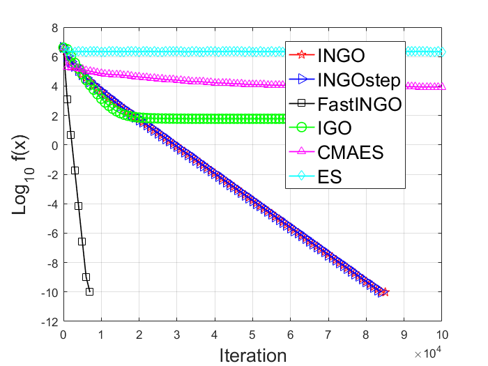
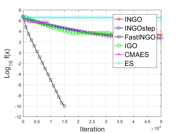
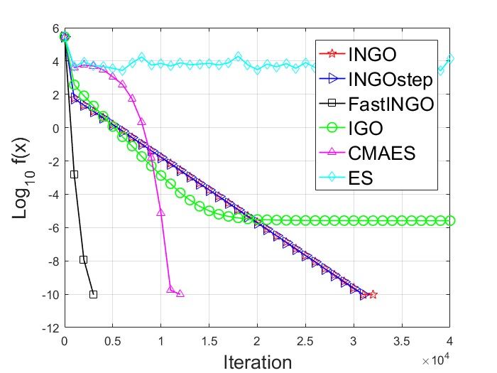
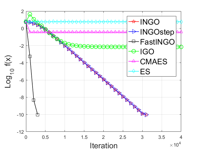
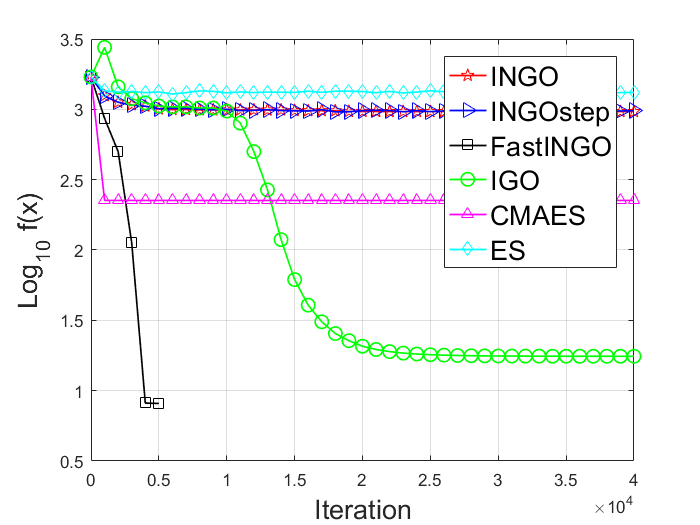
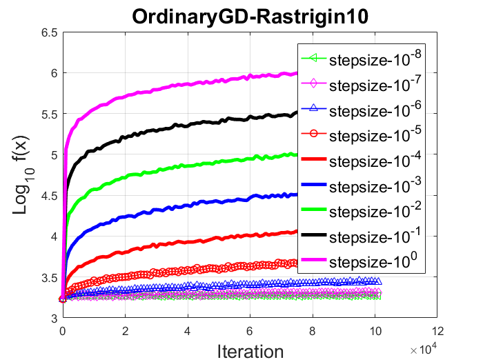
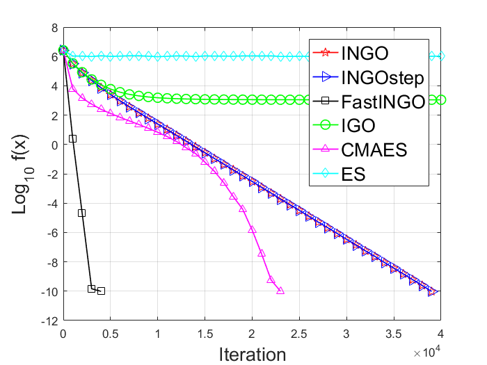
Figure 1: Mean value of fโ€‹(๐’™)๐‘“๐’™f(\boldsymbol{x}) in log10subscript10\log_{10} scale over 20 independent runs for 100-dimensional problems.
Refer to caption
(a) Swimmer
Refer to caption
(b) HalfCheetah
Refer to caption
(c) InvertedDoublePendulum
Refer to caption
(d) HumanoidStandup
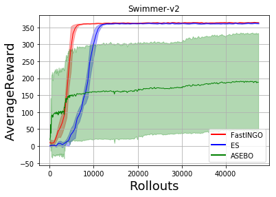
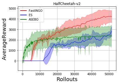
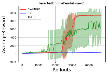
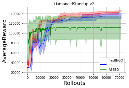
Figure 2: Average Reward over 5 independent runs on benchmark RL environments

Evaluation on synthetic continuous test benchmarks. We evaluate the proposed INGO , INGOstep and Fast-INGO (diagonal case of INGO) by comparing with one of the state-of-the-art method CMA-ESย [13] and IGOย [23] with full covariance matrix update, and vanilla ES with antithetic gradient estimatorsย [26] on several synthetic benchmark test problems. All the test problems are listed in Tableย 1 in the supplement.

Parameter Settings: For INGO, INGOstep and IGO, we use the same normalization transformation h(f(๐’™i)=fโ€‹(๐’™i)โˆ’ฮผ^ฯƒ^h(f({\boldsymbol{x}}_{i})=\frac{f({\boldsymbol{x}}_{i})-\widehat{\mu}}{\widehat{\sigma}} and all same hyper-parameters to test the effect of implicit natural gradient. We set step size ฮฒ=1/d๐›ฝ1๐‘‘\beta=1/d for all of them. For Fast-INGO, we set step size ฮฒ=1/d๐›ฝ1๐‘‘\beta=1/\sqrt{d}, where d๐‘‘d is the dimension of the test problems. The number of samples per iteration is set to N=2โ€‹โŒŠ3+โŒŠ3ร—lnโกdโŒ‹/2โŒ‹๐‘233๐‘‘2N=2\lfloor 3+\lfloor 3\times\ln{d}\rfloor/2\rfloor for all the methods, where โŒŠโ‹…โŒ‹โ‹…\lfloor\cdot\rfloor denotes the floor function. This setting ensures N๐‘N to be an even number. We set ๐ˆ1=0.5ร—๐Ÿsubscript๐ˆ10.51{\boldsymbol{\sigma}}_{1}=0.5\times{\boldsymbol{1}} and sample ๐1โˆผUโ€‹nโ€‹iโ€‹[๐ŸŽ,๐Ÿ]similar-tosubscript๐1๐‘ˆ๐‘›๐‘–01{\boldsymbol{\mu}}_{1}\sim Uni[{\boldsymbol{0}},{\boldsymbol{1}}] as the same initialization for all the methods, where Uโ€‹nโ€‹iโ€‹[0,1]๐‘ˆ๐‘›๐‘–01Uni[0,1] denotes the uniform distribution in [0,1]01[0,1]. For ESย [26], we use the default step-size hyper-parameters.

The mean value of fโ€‹(๐’™)๐‘“๐’™f(\boldsymbol{x}) over 20 independent runs for 100-dimensional problems are show in Figureย 1. From Figureย 1, we can see that INGO, INGOstep and Fast-INGO converge linearly in log scale. Fast-INGO can arrive 10โˆ’10superscript101010^{-10} precision on five cases except the highly non-convex Rastrigin10 problem. Fast-INGO employs the separate structure of the problems, thus it obtains better performance than the other methods with full matrix update. It is worth to note that Fast-INGO is not rotation invariant compared with Full-INGO. The INGO and INGOstep (with full matrix update) can arrive 10โˆ’10superscript101010^{-10} on four cases, while IGO with full matrix update can not achieve high precision. This shows that the update of inverse of covariance matrix is more stable. Moreover, CMA-ES converge linearly in log scale for the convex Ellipsoid problem but slower than Fast-INGO. In addition, CMAES converge slowly on the non-smooth โ„“1subscriptโ„“1\ell_{1}-Ellipsoid and the non-convex โ„“12subscriptโ„“12\ell_{\frac{1}{2}}-Ellipsoid problem. Furthermore, CMAES fails on the non-convex Levy problem, while INGO, INGOstep and Fast-INGO obtain 10โˆ’10superscript101010^{-10}. CMAES converges faster or achieves smaller value than ES. On the non-convex Rastrigin10 problem, all methods fail to obtain 10โˆ’10superscript101010^{-10} precision. Fast-INGO obtains smaller value. The results on synthetic test problems show that methods employing second-order information converge faster than first-order method ES. And employing second-order information is important to obtain high optimization precision, i.e., 10โˆ’10superscript101010^{-10}. Moreover, taking stochastic implicit natural gradient update can converge faster than IGO. The test functions are highly ill-conditioned and non-convex; the experimental results show that it is challenging for ES to optimize them well without adaptively update covariance and mean.

Evaluation on RL test problems. We further evaluate the proposed Fast-INGO by comparing AESBOย [10] and ES with antithetic gradient estimatorsย [26] on MuJoCo control problems: Swimmer, HalfCheetah, HumanoidStandup, InvertedDoublePendulum, in Open-AI Gym environments. CMA-ES is too slow due to the computation of eigendecomposition for high-dimensional problems.

We use one hidden layer feed-forward neural network with tanh activation function as policy architecture. The number of hidden unit is set to h=16โ„Ž16h=16 for all problems. The goal is to find the parameters of this policy network to achieve large reward. The same policy architecture is used for all the methods on all test problems. The number of samples per iteration is set to N=20+4โ€‹โŒŠโŒŠ3ร—lnโกdโŒ‹/2โŒ‹๐‘2043๐‘‘2N=20+4\lfloor\lfloor 3\times\ln{d}\rfloor/2\rfloor for all the methods. For Fast-INGO, we set step-size ฮฒ=0.3๐›ฝ0.3\beta=0.3 . We set ๐ˆ1=0.1ร—๐Ÿsubscript๐ˆ10.11{\boldsymbol{\sigma}}_{1}=0.1\times{\boldsymbol{1}} and ๐1=๐ŸŽsubscript๐10{\boldsymbol{\mu}}_{1}=\boldsymbol{0} as the initialization for both Fast-INGO and ES. For ESย [26], we use the default step-size hyper-parameters. Five independent runs are performed. The experimental results are shown in Figureย 2. We can observe that Fast-INGO increase AverageReward faster than ES on all four cases. This shows that the update using seconder order information in Fast-INGO can help accelerate convergence.

7 Conclusions

We proposed a novel stochastic implicit natural gradient frameworks for black-box optimization. Under this framework, we presented algorithms for both continuous and discrete black-box optimization. Theoretically, we proved the ๐’ชโ€‹(logโกT/T)๐’ช๐‘‡๐‘‡\mathcal{O}\left(\log T/T\right) convergence rate of our continuous algorithms with stochastic update for non-differentiable convex function under expectation ฮณ๐›พ\gamma-strongly convex assumption. We proved ๐’ชโ€‹(d2โ€‹logโกT/T)๐’ชsuperscript๐‘‘2๐‘‡๐‘‡\mathcal{O}\left(d^{2}\log T/T\right) converge rate for black-box function under same assumptions above. For isometric Gaussian case, we proved the ๐’ชโ€‹(dโ€‹logโกT/T)๐’ช๐‘‘๐‘‡๐‘‡\mathcal{O}\left(d\log T/T\right) converge rate when using d๐‘‘d orthogonal samples per iteration, which well supports parallel evaluation. Our method is very simple, and it contains less hyper-parameters than CMA-ES. Empirically, our methods obtain a competitive performance compared with CMA-ES. Moreover, our INGO and INGOstep with full matrix update can achieve high precision on Levy test problem and Ellipsoid problems, while IGOย [23] with full matrix update can not. This shows the efficiency of our methods. On RL control problems, our algorithms increase average reward faster than ASEBOย [10] and ES, which shows employing second order information can help accelerate convergence. Moreover, our discrete algorithm outperforms than GA on test functions.

References

  • [1] Youhei Akimoto, Yuichi Nagata, Isao Ono, and Shigenobu Kobayashi. Bidirectional relation between cma evolution strategies and natural evolution strategies. In International Conference on Parallel Problem Solving from Nature, pages 154โ€“163. Springer, 2010.
  • [2] Shun-Ichi Amari. Natural gradient works efficiently in learning. Neural computation, 10(2):251โ€“276, 1998.
  • [3] Shun-ichi Amari. Information geometry and its applications, volume 194. Springer, 2016.
  • [4] Katyย S Azoury and Manfredย K Warmuth. Relative loss bounds for on-line density estimation with the exponential family of distributions. Machine Learning, 43(3):211โ€“246, 2001.
  • [5] Thomas Back, Frank Hoffmeister, and Hans-Paul Schwefel. A survey of evolution strategies. In Proceedings of the fourth international conference on genetic algorithms, volumeย 2. Morgan Kaufmann Publishers San Mateo, CA, 1991.
  • [6] Krishnakumar Balasubramanian and Saeed Ghadimi. Zeroth-order (non)-convex stochastic optimization via conditional gradient and gradient updates. In Advances in Neural Information Processing Systems, pages 3455โ€“3464, 2018.
  • [7] Juanย Cruz Barsce, Jorgeย A Palombarini, and Ernestoย C Martรญnez. Towards autonomous reinforcement learning: Automatic setting of hyper-parameters using bayesian optimization. In Computer Conference (CLEI), 2017 XLIII Latin American, pages 1โ€“9. IEEE, 2017.
  • [8] Adamย D Bull. Convergence rates of efficient global optimization algorithms. Journal of Machine Learning Research (JMLR), 12(Oct):2879โ€“2904, 2011.
  • [9] Krzysztof Choromanski, Aldo Pacchiano, Jack Parker-Holder, and Yunhao Tang. From complexity to simplicity: Adaptive es-active subspaces for blackbox optimization. arXiv:1903.04268, 2019.
  • [10] Krzysztof Choromanski, Aldo Pacchiano, Jack Parker-Holder, Yunhao Tang, and Vikas Sindhwani. From complexity to simplicity: Adaptive es-active subspaces for blackbox optimization, 2019.
  • [11] Krzysztof Choromanski, Mark Rowland, Vikas Sindhwani, Richardย E Turner, and Adrian Weller. Structured evolution with compact architectures for scalable policy optimization. In ICML, pages 969โ€“977, 2018.
  • [12] Justin Domke. Provable smoothness guarantees for black-box variational inference. arXiv preprint arXiv:1901.08431, 2019.
  • [13] Nikolaus Hansen. The cma evolution strategy: a comparing review. In Towards a new evolutionary computation, pages 75โ€“102. Springer, 2006.
  • [14] Mohammadย Emtiyaz Khan and Wuย Lin. Conjugate-computation variational inference: Converting variational inference in non-conjugate models to inferences in conjugate models. arXiv preprint arXiv:1703.04265, 2017.
  • [15] Mohammadย Emtiyaz Khan and Didrik Nielsen. Fast yet simple natural-gradient descent for variational inference in complex models. In 2018 International Symposium on Information Theory and Its Applications (ISITA), pages 31โ€“35. IEEE, 2018.
  • [16] Mohammadย Emtiyaz Khan, Didrik Nielsen, Voot Tangkaratt, Wuย Lin, Yarin Gal, and Akash Srivastava. Fast and scalable bayesian deep learning by weight-perturbation in adam. In ICML, 2018.
  • [17] Guoqing Liu, Liย Zhao, Feidiao Yang, Jiang Bian, Tao Qin, Nenghai Yu, and Tie-Yan Liu. Trust region evolution strategies. In AAAI, 2019.
  • [18] Danielย J Lizotte, Tao Wang, Michaelย H Bowling, and Dale Schuurmans. Automatic gait optimization with gaussian process regression. In IJCAI, volumeย 7, pages 944โ€“949, 2007.
  • [19] Yueming Lyu. Spherical structured feature maps for kernel approximation. In Proceedings of the 34th International Conference on Machine Learning (ICML), pages 2256โ€“2264, 2017.
  • [20] Yueming Lyu, Yuan Yuan, and Ivorย W Tsang. Efficient batch black-box optimization with deterministic regret bounds. arXiv preprint arXiv:1905.10041, 2019.
  • [21] Dianaย M Negoescu, Peterย I Frazier, and Warrenย B Powell. The knowledge-gradient algorithm for sequencing experiments in drug discovery. INFORMS Journal on Computing, 23(3):346โ€“363, 2011.
  • [22] Yurii Nesterov and Vladimir Spokoiny. Random gradient-free minimization of convex functions. Foundations of Computational Mathematics, 17(2):527โ€“566, 2017.
  • [23] Yann Ollivier, Ludovic Arnold, Anne Auger, and Nikolaus Hansen. Information-geometric optimization algorithms: A unifying picture via invariance principles. The Journal of Machine Learning Research (JMLR), 18(1):564โ€“628, 2017.
  • [24] Garvesh Raskutti and Sayan Mukherjee. The information geometry of mirror descent. IEEE Transactions on Information Theory, 61(3):1451โ€“1457, 2015.
  • [25] Daniloย Jimenez Rezende, Shakir Mohamed, and Daan Wierstra. Stochastic backpropagation and approximate inference in deep generative models. In ICML, 2014.
  • [26] Tim Salimans, Jonathan Ho, Xiย Chen, Szymon Sidor, and Ilya Sutskever. Evolution strategies as a scalable alternative to reinforcement learning. arXiv preprint arXiv:1703.03864, 2017.
  • [27] Jasper Snoek, Hugo Larochelle, and Ryanย P Adams. Practical bayesian optimization of machine learning algorithms. In NeurIPS, pages 2951โ€“2959, 2012.
  • [28] Mandavilli Srinivas and Lalitย M Patnaik. Genetic algorithms: A survey. computer, 27(6):17โ€“26, 1994.
  • [29] Niranjan Srinivas, Andreas Krause, Shamย M Kakade, and Matthias Seeger. Gaussian process optimization in the bandit setting: No regret and experimental design. In ICML, 2010.
  • [30] Gย Gary Wang and Songqing Shan. Review of metamodeling techniques in support of engineering design optimization. Journal of Mechanical design, 129(4):370โ€“380, 2007.
  • [31] Daan Wierstra, Tom Schaul, Tobias Glasmachers, Yiย Sun, Jan Peters, and Jรผrgen Schmidhuber. Natural evolution strategies. The Journal of Machine Learning Research (JMLR), 15(1):949โ€“980, 2014.
  • [32] Zhiqiang Xu. Deterministic sampling of sparse trigonometric polynomials. Journal of Complexity, 27(2):133โ€“140, 2011.

Appendix A Optimization for Discrete Variable

Binary Optimization: For function fโ€‹(๐’™)๐‘“๐’™f(\boldsymbol{x}) over binary variable ๐’™โˆˆ{0,1}d๐’™superscript01๐‘‘\boldsymbol{x}\in\{0,1\}^{d}, we employ Bernoulli distribution with parameter ๐’‘=[p1,โ‹ฏ,pd]โŠค๐’‘superscriptsubscript๐‘1โ‹ฏsubscript๐‘๐‘‘top\boldsymbol{\boldsymbol{p}}=[p_{1},\cdots,p_{d}]^{\top} as the underlying distribution, where pisubscript๐‘๐‘–p_{i} denote the probability of xi=1subscript๐‘ฅ๐‘–1x_{i}=1. Let ๐œผ๐œผ\boldsymbol{\eta} denote the natural parameter, then we know ๐’‘=11+eโˆ’๐œผ๐’‘11superscript๐‘’๐œผ\boldsymbol{\boldsymbol{p}}=\frac{1}{1+e^{-\boldsymbol{\eta}}}. The mean parameter is ๐’Ž=๐’‘๐’Ž๐’‘{\boldsymbol{m}}={\boldsymbol{p}}.

From Eq.(4), we know that

๐œผt+1=๐œผtโˆ’ฮฒtโ€‹โˆ‡๐’‘๐”ผ๐’‘โ€‹[fโ€‹(๐’™)]subscript๐œผ๐‘ก1subscript๐œผ๐‘กsubscript๐›ฝ๐‘กsubscriptโˆ‡๐’‘subscript๐”ผ๐’‘delimited-[]๐‘“๐’™\displaystyle\boldsymbol{\eta}_{t+1}=\boldsymbol{\eta}_{t}-\beta_{t}\nabla_{\boldsymbol{p}}\mathbb{E}_{\boldsymbol{p}}[f(\boldsymbol{x})] (33)

Approximate the gradient by Monte Carlo sampling, we obtain that

๐œผt+1=๐œผtโˆ’ฮฒtโ€‹1Nโ€‹โˆ‘n=1Nfโ€‹(๐’™n)โ€‹๐’‰nsubscript๐œผ๐‘ก1subscript๐œผ๐‘กsubscript๐›ฝ๐‘ก1๐‘superscriptsubscript๐‘›1๐‘๐‘“superscript๐’™๐‘›superscript๐’‰๐‘›\displaystyle\boldsymbol{\eta}_{t+1}=\boldsymbol{\eta}_{t}-\beta_{t}\frac{1}{N}\sum_{n=1}^{N}f(\boldsymbol{x}^{n})\boldsymbol{h}^{n} (34)

where ๐’‰in=1piโ€‹๐Ÿโ€‹(๐’™in=1)โˆ’11โˆ’piโ€‹๐Ÿโ€‹(๐’™in=0)subscriptsuperscript๐’‰๐‘›๐‘–1subscript๐‘๐‘–1subscriptsuperscript๐’™๐‘›๐‘–111subscript๐‘๐‘–1subscriptsuperscript๐’™๐‘›๐‘–0\boldsymbol{h}^{n}_{i}=\frac{1}{p_{i}}\boldsymbol{1}(\boldsymbol{x}^{n}_{i}=1)-\frac{1}{1-p_{i}}\boldsymbol{1}(\boldsymbol{x}^{n}_{i}=0).

In order to achieve stable update, we normalize function value by its mean ฮผ^^๐œ‡\widehat{\mu} and standard deviation ฯƒ^^๐œŽ\widehat{\sigma} in a batch. The normalized update is given as follows.

๐œผt+1=๐œผtโˆ’ฮฒtโ€‹โˆ‘n=1Nfโ€‹(๐’™n)โˆ’ฮผ^Nโ€‹ฯƒ^โ€‹๐’‰nsubscript๐œผ๐‘ก1subscript๐œผ๐‘กsubscript๐›ฝ๐‘กsuperscriptsubscript๐‘›1๐‘๐‘“superscript๐’™๐‘›^๐œ‡๐‘^๐œŽsuperscript๐’‰๐‘›\displaystyle\boldsymbol{\eta}_{t+1}=\boldsymbol{\eta}_{t}-\beta_{t}\sum_{n=1}^{N}\frac{f(\boldsymbol{x}^{n})-\widehat{\mu}}{N\widehat{\sigma}}\boldsymbol{h}^{n} (35)

General Discrete Optimization: Similarly, for function fโ€‹(๐’™)๐‘“๐’™f(\boldsymbol{x}) over discrete variable ๐’™โˆˆ{1,โ‹ฏ,K}d๐’™superscript1โ‹ฏ๐พ๐‘‘\boldsymbol{x}\in\{1,\cdots,K\}^{d}, we employ categorical distribution with parameter ๐‘ท=[๐’‘1,โ‹ฏ,๐’‘d]โŠค๐‘ทsuperscriptsubscript๐’‘1โ‹ฏsubscript๐’‘๐‘‘top\boldsymbol{\boldsymbol{P}}=[\boldsymbol{p}_{1},\cdots,\boldsymbol{p}_{d}]^{\top} as the underlying distribution, where the iโ€‹j๐‘–๐‘—{ij}-th element of ๐‘ท๐‘ท\boldsymbol{P} (๐‘ทiโ€‹jsubscript๐‘ท๐‘–๐‘—\boldsymbol{P}_{ij}) denote the probability of ๐’™i=jsubscript๐’™๐‘–๐‘—\boldsymbol{x}_{i}=j. Let ๐œผโˆˆโ„›dร—K๐œผsuperscriptโ„›๐‘‘๐พ\boldsymbol{\eta}\in\mathcal{R}^{d\times K} denote the natural parameter, then we know ๐‘ทiโ€‹j=e๐œผiโ€‹jโˆ‘j=1Ke๐œผiโ€‹jsubscript๐‘ท๐‘–๐‘—superscript๐‘’subscript๐œผ๐‘–๐‘—superscriptsubscript๐‘—1๐พsuperscript๐‘’subscript๐œผ๐‘–๐‘—\boldsymbol{P}_{ij}=\frac{e^{\boldsymbol{\eta}_{ij}}}{\sum_{j=1}^{K}{e^{\boldsymbol{\eta}_{ij}}}}. The mean parameter is ๐’Ž=๐‘ท๐’Ž๐‘ท{\boldsymbol{m}}={\boldsymbol{P}}.

From Eq.(4), we know that

๐œผt+1=๐œผtโˆ’ฮฒtโ€‹โˆ‡๐‘ท๐”ผ๐‘ทโ€‹[fโ€‹(๐’™)]subscript๐œผ๐‘ก1subscript๐œผ๐‘กsubscript๐›ฝ๐‘กsubscriptโˆ‡๐‘ทsubscript๐”ผ๐‘ทdelimited-[]๐‘“๐’™\displaystyle\boldsymbol{\eta}_{t+1}=\boldsymbol{\eta}_{t}-\beta_{t}\nabla_{\boldsymbol{P}}\mathbb{E}_{\boldsymbol{P}}[f(\boldsymbol{x})] (36)

Approximate the gradient by Monte Carlo sampling,

๐œผt+1=๐œผtโˆ’ฮฒtโ€‹1Nโ€‹โˆ‘n=1Nfโ€‹(๐’™n)โ€‹๐‘ฏnsubscript๐œผ๐‘ก1subscript๐œผ๐‘กsubscript๐›ฝ๐‘ก1๐‘superscriptsubscript๐‘›1๐‘๐‘“superscript๐’™๐‘›superscript๐‘ฏ๐‘›\displaystyle\boldsymbol{\eta}_{t+1}=\boldsymbol{\eta}_{t}-\beta_{t}\frac{1}{N}\sum_{n=1}^{N}f(\boldsymbol{x}^{n})\boldsymbol{H}^{n} (37)

where ๐‘ฏiโ€‹jn=1๐‘ทiโ€‹jโ€‹๐Ÿโ€‹(๐’™in=j)subscriptsuperscript๐‘ฏ๐‘›๐‘–๐‘—1subscript๐‘ท๐‘–๐‘—1subscriptsuperscript๐’™๐‘›๐‘–๐‘—\boldsymbol{H}^{n}_{ij}=\frac{1}{\boldsymbol{P}_{ij}}\boldsymbol{1}(\boldsymbol{x}^{n}_{i}=j). We can also normalize the update by the mean ฮผ^^๐œ‡\widehat{\mu} and std ฯƒ^^๐œŽ\widehat{\sigma}.

Evaluation on discrete test problems

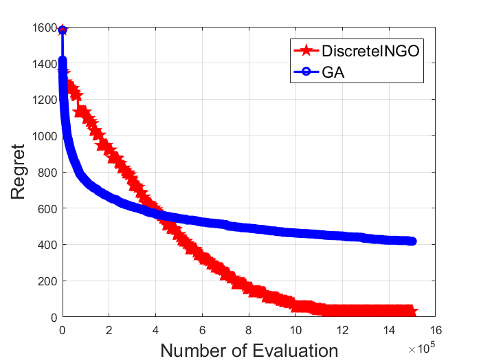
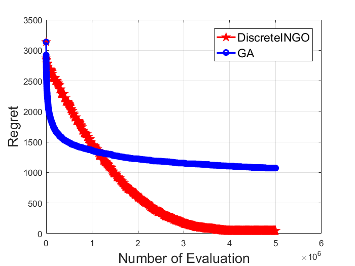
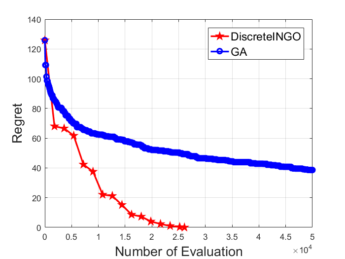
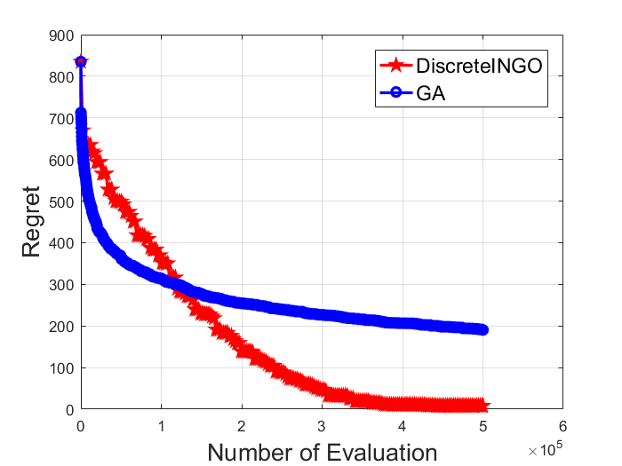
We evaluate our discrete INGO by comparing with GA method on binary reconstruction benchmark problem, i.e., fโ€‹(๐’™):=โ€–signโ€‹(๐’™โˆ’0.5)โˆ’๐’˜โ€–22โˆ’โ€–signโ€‹(๐’˜)โˆ’๐’˜โ€–22assign๐‘“๐’™subscriptsuperscriptnormsign๐’™0.5๐’˜22subscriptsuperscriptnormsign๐’˜๐’˜22f(\boldsymbol{x}):=\|\text{sign}(\boldsymbol{x}-0.5)-\boldsymbol{w}\|^{2}_{2}-\|\text{sign}(\boldsymbol{w})-\boldsymbol{w}\|^{2}_{2} with ๐’™โˆˆ{0,1}d๐’™superscript01๐‘‘\boldsymbol{x}\in\{0,1\}^{d} . We construct ๐’˜๐’˜\boldsymbol{w} by sampling from standard Gaussian. The dimension d๐‘‘d of test problem is set to {100,500,1000,2000}10050010002000\{100,500,1000,2000\}, respectively. For our discrete INGO, we set the stepsize ฮฒ=1/d๐›ฝ1๐‘‘\beta=1/d. The number of samples per iteration is same as INGO, i.e., N=20+4โ€‹โŒŠ3+โŒŠ3ร—lnโกdโŒ‹/2โŒ‹๐‘20433๐‘‘2N=20+4\lfloor 3+\lfloor 3\times\ln{d}\rfloor/2\rfloor.

The experimental resutls are shown in Fig.ย 3. We can observe that our discrete INGO achieves much smaller regret compared with GA. Our discrete INGO converges to near zero regret on test problems, while GA decrease very slowly after a short initial greedy phase.
Refer to caption
(a) 100-dimensional problem
Refer to caption
(b) 500-dimensional problem
Refer to caption
(c) 1000-dimensional problem
Refer to caption
(d) 2000-dimensional problem
Figure 3: Mean value of regret over 10 independent runs for different dimensional discrete optimization problems

Appendix B Proof of Theorem 2

Proof.

For Gaussian distribution p:=๐’ฉโ€‹(๐,ฮฃ)assign๐‘๐’ฉ๐ฮฃp:=\mathcal{N}({\boldsymbol{\mu}},\Sigma), the gradient of ๐”ผpโ€‹[fโ€‹(๐’™)]subscript๐”ผ๐‘delimited-[]๐‘“๐’™\mathbb{E}_{p}[f({\boldsymbol{x}})] w.r.t ๐๐{\boldsymbol{\mu}} can be derived as follows:

โˆ‡๐๐”ผpโ€‹[fโ€‹(๐’™)]subscriptโˆ‡๐subscript๐”ผ๐‘delimited-[]๐‘“๐’™\displaystyle\nabla_{\boldsymbol{\mu}}\mathbb{E}_{p}[f({\boldsymbol{x}})] =๐”ผpโ€‹[fโ€‹(๐’™)โ€‹โˆ‡๐logโก(pโ€‹(๐’™;๐,ฮฃ))]absentsubscript๐”ผ๐‘delimited-[]๐‘“๐’™subscriptโˆ‡๐๐‘๐’™๐ฮฃ\displaystyle=\mathbb{E}_{p}[f({\boldsymbol{x}})\nabla_{\boldsymbol{\mu}}\log(p({\boldsymbol{x}};\boldsymbol{\mu},\Sigma))] (38)
=๐”ผpโ€‹[fโ€‹(๐’™)โ€‹โˆ‡๐[โˆ’12โ€‹(๐’™โˆ’๐)โŠคโ€‹ฮฃโˆ’1โ€‹(๐’™โˆ’๐)]]absentsubscript๐”ผ๐‘delimited-[]๐‘“๐’™subscriptโˆ‡๐12superscript๐’™๐topsuperscriptฮฃ1๐’™๐\displaystyle=\mathbb{E}_{p}\left[f({\boldsymbol{x}})\nabla_{\boldsymbol{\mu}}\left[-\frac{1}{2}({\boldsymbol{x}}-{\boldsymbol{\mu}})^{\top}\Sigma^{-1}({\boldsymbol{x}}-{\boldsymbol{\mu}})\right]\right] (39)
=๐”ผpโ€‹[ฮฃโˆ’1โ€‹(๐’™โˆ’๐)โ€‹fโ€‹(๐’™)]absentsubscript๐”ผ๐‘delimited-[]superscriptฮฃ1๐’™๐๐‘“๐’™\displaystyle=\mathbb{E}_{p}\left[\Sigma^{-1}({\boldsymbol{x}}-{\boldsymbol{\mu}})f({\boldsymbol{x}})\right] (40)

The gradient of ๐”ผpโ€‹[fโ€‹(๐’™)]subscript๐”ผ๐‘delimited-[]๐‘“๐’™\mathbb{E}_{p}[f({\boldsymbol{x}})] w.r.t ฮฃฮฃ\Sigma can be derived as follows:

โˆ‡ฮฃ๐”ผpโ€‹[fโ€‹(๐’™)]subscriptโˆ‡ฮฃsubscript๐”ผ๐‘delimited-[]๐‘“๐’™\displaystyle\nabla_{\Sigma}\mathbb{E}_{p}[f({\boldsymbol{x}})] =๐”ผpโ€‹[fโ€‹(๐’™)โ€‹โˆ‡ฮฃlogโก(pโ€‹(๐’™;๐,ฮฃ))]absentsubscript๐”ผ๐‘delimited-[]๐‘“๐’™subscriptโˆ‡ฮฃ๐‘๐’™๐ฮฃ\displaystyle=\mathbb{E}_{p}[f({\boldsymbol{x}})\nabla_{\Sigma}\log(p({\boldsymbol{x}};\boldsymbol{\mu},\Sigma))] (41)
=๐”ผpโ€‹[fโ€‹(๐’™)โ€‹โˆ‡ฮฃ[โˆ’12โ€‹(๐’™โˆ’๐)โŠคโ€‹ฮฃโˆ’1โ€‹(๐’™โˆ’๐)โˆ’12โ€‹logโกdetโ€‹(ฮฃ)]]absentsubscript๐”ผ๐‘delimited-[]๐‘“๐’™subscriptโˆ‡ฮฃ12superscript๐’™๐topsuperscriptฮฃ1๐’™๐12detฮฃ\displaystyle=\mathbb{E}_{p}\left[f({\boldsymbol{x}})\nabla_{\Sigma}\left[-\frac{1}{2}({\boldsymbol{x}}-{\boldsymbol{\mu}})^{\top}\Sigma^{-1}({\boldsymbol{x}}-{\boldsymbol{\mu}})-\frac{1}{2}\log\text{det}(\Sigma)\right]\right] (42)
=12โ€‹๐”ผpโ€‹[(ฮฃโˆ’1โ€‹(๐’™โˆ’๐)โ€‹(๐’™โˆ’๐)โŠคโ€‹ฮฃโˆ’1โˆ’ฮฃโˆ’1)โ€‹fโ€‹(๐’™)]absent12subscript๐”ผ๐‘delimited-[]superscriptฮฃ1๐’™๐superscript๐’™๐topsuperscriptฮฃ1superscriptฮฃ1๐‘“๐’™\displaystyle=\frac{1}{2}\mathbb{E}_{p}\left[\left(\Sigma^{-1}({\boldsymbol{x}}-{\boldsymbol{\mu}})({\boldsymbol{x}}-{\boldsymbol{\mu}})^{\top}\Sigma^{-1}\!\!-\!\!\Sigma^{-1}\right)f({\boldsymbol{x}})\right] (43)

โˆŽ

Appendix C Proof of Theorem B

Theorem.

Suppose fโ€‹(๐ฑ)๐‘“๐ฑf({\boldsymbol{x}}) be an integrable and twice differentiable function under a Gaussian distribution p:=๐’ฉโ€‹(๐›,ฮฃ)assign๐‘๐’ฉ๐›ฮฃp:=\mathcal{N}({\boldsymbol{\mu}},\Sigma) such that ๐”ผpโ€‹[โˆ‡๐ฑfโ€‹(๐ฑ)]subscript๐”ผ๐‘delimited-[]subscriptโˆ‡๐ฑ๐‘“๐ฑ\mathbb{E}_{p}\left[\nabla_{\boldsymbol{x}}f({\boldsymbol{x}})\right] and ๐”ผpโ€‹[โˆ‚2fโ€‹(๐ฑ)โˆ‚๐ฑโ€‹โˆ‚๐ฑโŠค]subscript๐”ผ๐‘delimited-[]superscript2๐‘“๐ฑ๐ฑsuperscript๐ฑtop\mathbb{E}_{p}\left[\frac{\partial^{2}f({\boldsymbol{x}})}{\partial{\boldsymbol{x}}\partial{\boldsymbol{x}}^{\top}}\right] exists. Then, the expectation of the gradient and Hessian of fโ€‹(๐ฑ)๐‘“๐ฑf({\boldsymbol{x}}) can be expressed as Eq.(44) and Eq.(45), respectively.

๐”ผpโ€‹[โˆ‡๐’™fโ€‹(๐’™)]=๐”ผpโ€‹[ฮฃโˆ’1โ€‹(๐’™โˆ’๐)โ€‹fโ€‹(๐’™)]subscript๐”ผ๐‘delimited-[]subscriptโˆ‡๐’™๐‘“๐’™subscript๐”ผ๐‘delimited-[]superscriptฮฃ1๐’™๐๐‘“๐’™\displaystyle\mathbb{E}_{p}\left[\nabla_{\boldsymbol{x}}f({\boldsymbol{x}})\right]=\mathbb{E}_{p}\left[\Sigma^{-1}({\boldsymbol{x}}-{\boldsymbol{\mu}})f({\boldsymbol{x}})\right] (44)
๐”ผpโ€‹[โˆ‚2fโ€‹(๐’™)โˆ‚๐’™โ€‹โˆ‚๐’™โŠค]=๐”ผpโ€‹[(ฮฃโˆ’1โ€‹(๐’™โˆ’๐)โ€‹(๐’™โˆ’๐)โŠคโ€‹ฮฃโˆ’1โˆ’ฮฃโˆ’1)โ€‹fโ€‹(๐’™)]subscript๐”ผ๐‘delimited-[]superscript2๐‘“๐’™๐’™superscript๐’™topsubscript๐”ผ๐‘delimited-[]superscriptฮฃ1๐’™๐superscript๐’™๐topsuperscriptฮฃ1superscriptฮฃ1๐‘“๐’™\displaystyle\mathbb{E}_{p}\left[\frac{\partial^{2}f({\boldsymbol{x}})}{\partial{\boldsymbol{x}}\partial{\boldsymbol{x}}^{\top}}\right]=\mathbb{E}_{p}\left[\left(\Sigma^{-1}({\boldsymbol{x}}-{\boldsymbol{\mu}})({\boldsymbol{x}}-{\boldsymbol{\mu}})^{\top}\Sigma^{-1}\!\!-\!\!\Sigma^{-1}\right)f({\boldsymbol{x}})\right] (45)
Proof.

For Gaussian distribution, from Bonnetโ€™s theoremย [25], we know that

โˆ‡๐๐”ผp[f(๐’™)]=๐”ผp[โˆ‡๐’™f(๐’™)]].\displaystyle\nabla_{\boldsymbol{\mu}}\mathbb{E}_{p}[f({\boldsymbol{x}})]=\mathbb{E}_{p}\left[\nabla_{\boldsymbol{x}}f({\boldsymbol{x}})\right]]. (46)

From Theorem 2, we know that

โˆ‡๐๐”ผpโ€‹[fโ€‹(๐’™)]=๐”ผpโ€‹[ฮฃโˆ’1โ€‹(๐’™โˆ’๐)โ€‹fโ€‹(๐’™)].subscriptโˆ‡๐subscript๐”ผ๐‘delimited-[]๐‘“๐’™subscript๐”ผ๐‘delimited-[]superscriptฮฃ1๐’™๐๐‘“๐’™\displaystyle\nabla_{\boldsymbol{\mu}}\mathbb{E}_{p}[f({\boldsymbol{x}})]=\mathbb{E}_{p}\left[\Sigma^{-1}({\boldsymbol{x}}-{\boldsymbol{\mu}})f({\boldsymbol{x}})\right]. (47)

Thus, we can obtain that

๐”ผpโ€‹[โˆ‡๐’™fโ€‹(๐’™)]=๐”ผpโ€‹[ฮฃโˆ’1โ€‹(๐’™โˆ’๐)โ€‹fโ€‹(๐’™)].subscript๐”ผ๐‘delimited-[]subscriptโˆ‡๐’™๐‘“๐’™subscript๐”ผ๐‘delimited-[]superscriptฮฃ1๐’™๐๐‘“๐’™\displaystyle\mathbb{E}_{p}\left[\nabla_{\boldsymbol{x}}f({\boldsymbol{x}})\right]=\mathbb{E}_{p}\left[\Sigma^{-1}({\boldsymbol{x}}-{\boldsymbol{\mu}})f({\boldsymbol{x}})\right]. (48)

From Priceโ€™s Theoremย [25], we know that

โˆ‡ฮฃ๐”ผpโ€‹[fโ€‹(๐’™)]=12โ€‹๐”ผpโ€‹[โˆ‚2fโ€‹(๐’™)โˆ‚๐’™โ€‹โˆ‚๐’™โŠค].subscriptโˆ‡ฮฃsubscript๐”ผ๐‘delimited-[]๐‘“๐’™12subscript๐”ผ๐‘delimited-[]superscript2๐‘“๐’™๐’™superscript๐’™top\displaystyle\nabla_{\Sigma}\mathbb{E}_{p}[f({\boldsymbol{x}})]=\frac{1}{2}\mathbb{E}_{p}\left[\frac{\partial^{2}f({\boldsymbol{x}})}{\partial{\boldsymbol{x}}\partial{\boldsymbol{x}}^{\top}}\right]. (49)

From Theorem 2, we know that

โˆ‡ฮฃ๐”ผpโ€‹[fโ€‹(๐’™)]=12โ€‹๐”ผpโ€‹[(ฮฃโˆ’1โ€‹(๐’™โˆ’๐)โ€‹(๐’™โˆ’๐)โŠคโ€‹ฮฃโˆ’1โˆ’ฮฃโˆ’1)โ€‹fโ€‹(๐’™)]subscriptโˆ‡ฮฃsubscript๐”ผ๐‘delimited-[]๐‘“๐’™12subscript๐”ผ๐‘delimited-[]superscriptฮฃ1๐’™๐superscript๐’™๐topsuperscriptฮฃ1superscriptฮฃ1๐‘“๐’™\displaystyle\nabla_{\Sigma}\mathbb{E}_{p}[f({\boldsymbol{x}})]=\frac{1}{2}\mathbb{E}_{p}\left[\left(\Sigma^{-1}({\boldsymbol{x}}-{\boldsymbol{\mu}})({\boldsymbol{x}}-{\boldsymbol{\mu}})^{\top}\Sigma^{-1}\!\!-\!\!\Sigma^{-1}\right)f({\boldsymbol{x}})\right] (50)

It follows that

๐”ผpโ€‹[โˆ‚2fโ€‹(๐’™)โˆ‚๐’™โ€‹โˆ‚๐’™โŠค]=๐”ผpโ€‹[(ฮฃโˆ’1โ€‹(๐’™โˆ’๐)โ€‹(๐’™โˆ’๐)โŠคโ€‹ฮฃโˆ’1โˆ’ฮฃโˆ’1)โ€‹fโ€‹(๐’™)]subscript๐”ผ๐‘delimited-[]superscript2๐‘“๐’™๐’™superscript๐’™topsubscript๐”ผ๐‘delimited-[]superscriptฮฃ1๐’™๐superscript๐’™๐topsuperscriptฮฃ1superscriptฮฃ1๐‘“๐’™\displaystyle\mathbb{E}_{p}\left[\frac{\partial^{2}f({\boldsymbol{x}})}{\partial{\boldsymbol{x}}\partial{\boldsymbol{x}}^{\top}}\right]=\mathbb{E}_{p}\left[\left(\Sigma^{-1}({\boldsymbol{x}}-{\boldsymbol{\mu}})({\boldsymbol{x}}-{\boldsymbol{\mu}})^{\top}\Sigma^{-1}\!\!-\!\!\Sigma^{-1}\right)f({\boldsymbol{x}})\right] (51)

โˆŽ

Appendix D Proof of Theorem 3

Proof.

For Guassian distribution with parameter ๐œฝ:={๐,ฮฃ}assign๐œฝ๐ฮฃ{\boldsymbol{\theta}}:=\{{\boldsymbol{\mu}},\Sigma\}, problemย (20) can be rewrited as

โŸจ๐œฝ,โˆ‡๐œฝJยฏโ€‹(๐œฝt)โŸฉ+1ฮฒtโ€‹KLโ€‹(pฮธโˆฅpฮธt)๐œฝsubscriptโˆ‡๐œฝยฏ๐ฝsubscript๐œฝ๐‘ก1subscript๐›ฝ๐‘กKLconditionalsubscript๐‘๐œƒsubscript๐‘subscript๐œƒ๐‘ก\displaystyle\left<{\boldsymbol{\theta}},\nabla_{\boldsymbol{\theta}}\bar{J}({\boldsymbol{\theta}_{t}})\right>\!+\!\frac{1}{\beta_{t}}\text{KL}\left(p_{\theta}\|p_{\theta_{t}}\right) =๐โŠคโ€‹โˆ‡๐Jยฏโ€‹(๐œฝt)+trโ€‹(ฮฃโ€‹โˆ‡ฮฃJยฏโ€‹(๐œฝt))absentsuperscript๐topsubscriptโˆ‡๐ยฏ๐ฝsubscript๐œฝ๐‘กtrฮฃsubscriptโˆ‡ฮฃยฏ๐ฝsubscript๐œฝ๐‘ก\displaystyle={\boldsymbol{\mu}}^{\top}\nabla_{\boldsymbol{\mu}}\bar{J}({\boldsymbol{\theta}}_{t})\!+\!\text{tr}(\Sigma\nabla_{\Sigma}\bar{J}({\boldsymbol{\theta}}_{t}))
+12โ€‹ฮฒtโ€‹[trโ€‹(ฮฃtโˆ’1โ€‹ฮฃ)+(๐โˆ’๐t)โŠคโ€‹ฮฃtโˆ’1โ€‹(๐โˆ’๐t)+logโก|ฮฃt||ฮฃ|โˆ’d]12subscript๐›ฝ๐‘กdelimited-[]trsuperscriptsubscriptฮฃ๐‘ก1ฮฃsuperscript๐subscript๐๐‘กtopsuperscriptsubscriptฮฃ๐‘ก1๐subscript๐๐‘กsubscriptฮฃ๐‘กฮฃ๐‘‘\displaystyle+\frac{1}{2\beta_{t}}\!\left[\text{tr}(\Sigma_{t}^{-1}\Sigma)\!+\!({\boldsymbol{\mu}}\!-\!{\boldsymbol{\mu}}_{t})^{\top}\Sigma_{t}^{-1}({\boldsymbol{\mu}}\!-\!{\boldsymbol{\mu}}_{t})\!+\!\log\!{\frac{|\Sigma_{t}|}{|\Sigma|}}\!-\!d\right] (52)

where โˆ‡๐Jยฏโ€‹(๐œฝt)subscriptโˆ‡๐ยฏ๐ฝsubscript๐œฝ๐‘ก\nabla_{\boldsymbol{\mu}}\bar{J}({\boldsymbol{\theta}}_{t}) denotes the derivative w.r.t ๐๐{\boldsymbol{\mu}} taking at ๐=๐t,ฮฃ=ฮฃtformulae-sequence๐subscript๐๐‘กฮฃsubscriptฮฃ๐‘ก{\boldsymbol{\mu}}={\boldsymbol{\mu}}_{t},\Sigma=\Sigma_{t}. โˆ‡ฮฃJยฏโ€‹(๐œฝt)subscriptโˆ‡ฮฃยฏ๐ฝsubscript๐œฝ๐‘ก\nabla_{\Sigma}\bar{J}({\boldsymbol{\theta}}_{t}) denotes the derivative w.r.t ฮฃฮฃ\Sigma taking at ๐=๐t,ฮฃ=ฮฃtformulae-sequence๐subscript๐๐‘กฮฃsubscriptฮฃ๐‘ก{\boldsymbol{\mu}}={\boldsymbol{\mu}}_{t},\Sigma=\Sigma_{t}. Note that โˆ‡๐Jยฏโ€‹(๐œฝt)subscriptโˆ‡๐ยฏ๐ฝsubscript๐œฝ๐‘ก\nabla_{\boldsymbol{\mu}}\bar{J}({\boldsymbol{\theta}}_{t}) and โˆ‡ฮฃJยฏโ€‹(๐œฝt)subscriptโˆ‡ฮฃยฏ๐ฝsubscript๐œฝ๐‘ก\nabla_{\Sigma}\bar{J}({\boldsymbol{\theta}}_{t}) are not functions now.

From Eq.(52), we can see that the problem is convex with respect to ๐๐{\boldsymbol{\mu}} and ฮฃฮฃ\Sigma. Taking the derivative of (52) w.r.t ๐๐{\boldsymbol{\mu}} and ฮฃฮฃ\Sigma, and setting them to zero, we can obtain that

โˆ‡๐Jยฏโ€‹(๐œฝt)+1ฮฒtโ€‹ฮฃtโˆ’1โ€‹(๐โˆ’๐t)=๐ŸŽsubscriptโˆ‡๐ยฏ๐ฝsubscript๐œฝ๐‘ก1subscript๐›ฝ๐‘กsuperscriptsubscriptฮฃ๐‘ก1๐subscript๐๐‘ก0\displaystyle\nabla_{\boldsymbol{\mu}}\bar{J}({\boldsymbol{\theta}}_{t})+\frac{1}{\beta_{t}}\Sigma_{t}^{-1}({\boldsymbol{\mu}}\!-\!{\boldsymbol{\mu}}_{t})={\boldsymbol{0}} (53)
โˆ‡ฮฃJยฏ(๐œฝt))+12โ€‹ฮฒt[ฮฃtโˆ’1โˆ’ฮฃโˆ’1]=๐ŸŽ\displaystyle\nabla_{\Sigma}\bar{J}({\boldsymbol{\theta}}_{t}))+\frac{1}{2\beta_{t}}\left[\Sigma_{t}^{-1}-\Sigma^{-1}\right]={\boldsymbol{0}} (54)

It follows that

๐=๐tโˆ’ฮฒtโ€‹ฮฃtโ€‹โˆ‡๐Jยฏโ€‹(๐œฝt)๐subscript๐๐‘กsubscript๐›ฝ๐‘กsubscriptฮฃ๐‘กsubscriptโˆ‡๐ยฏ๐ฝsubscript๐œฝ๐‘ก\displaystyle{\boldsymbol{\mu}}={\boldsymbol{\mu}}_{t}-\beta_{t}\Sigma_{t}\nabla_{\boldsymbol{\mu}}\bar{J}({\boldsymbol{\theta}}_{t}) (55)
ฮฃโˆ’1=ฮฃtโˆ’1+2โ€‹ฮฒtโ€‹โˆ‡ฮฃJยฏโ€‹(๐œฝt)superscriptฮฃ1subscriptsuperscriptฮฃ1๐‘ก2subscript๐›ฝ๐‘กsubscriptโˆ‡ฮฃยฏ๐ฝsubscript๐œฝ๐‘ก\displaystyle\Sigma^{-1}=\Sigma^{-1}_{t}+2\beta_{t}\nabla_{\Sigma}\bar{J}({\boldsymbol{\theta}}_{t}) (56)

By definition, ๐t+1subscript๐๐‘ก1{\boldsymbol{\mu}}_{t+1} and ฮฃt+1subscriptฮฃ๐‘ก1\Sigma_{t+1} are the optimum of this convex optimization problem. Thus, we achieve that

๐t+1=๐tโˆ’ฮฒtโ€‹ฮฃtโ€‹โˆ‡๐Jยฏโ€‹(๐œฝt)subscript๐๐‘ก1subscript๐๐‘กsubscript๐›ฝ๐‘กsubscriptฮฃ๐‘กsubscriptโˆ‡๐ยฏ๐ฝsubscript๐œฝ๐‘ก\displaystyle{\boldsymbol{\mu}}_{t+1}={\boldsymbol{\mu}}_{t}-\beta_{t}\Sigma_{t}\nabla_{\boldsymbol{\mu}}\bar{J}({\boldsymbol{\theta}}_{t}) (57)
ฮฃt+1โˆ’1=ฮฃtโˆ’1+2โ€‹ฮฒtโ€‹โˆ‡ฮฃJยฏโ€‹(๐œฝt)subscriptsuperscriptฮฃ1๐‘ก1subscriptsuperscriptฮฃ1๐‘ก2subscript๐›ฝ๐‘กsubscriptโˆ‡ฮฃยฏ๐ฝsubscript๐œฝ๐‘ก\displaystyle\Sigma^{-1}_{t+1}=\Sigma^{-1}_{t}+2\beta_{t}\nabla_{\Sigma}\bar{J}({\boldsymbol{\theta}}_{t}) (58)

โˆŽ

Appendix E Proof of Theorem D

Theorem.

For Gaussian distribution with parameter ๐ฆ:={๐ฆ1,๐ฆ2}={๐›,ฮฃ+๐›โ€‹๐›โŠค}assign๐ฆsubscript๐ฆ1subscript๐ฆ2๐›ฮฃ๐›superscript๐›top{\boldsymbol{m}}:=\{{\boldsymbol{m}}_{1},{\boldsymbol{m}}_{2}\}=\{{\boldsymbol{\mu}},\Sigma+{\boldsymbol{\mu}}{\boldsymbol{\mu}}^{\top}\}, let v^t={g^tโˆ’2โ€‹G^tโ€‹๐›t,G^t}subscript^๐‘ฃ๐‘กsubscript^๐‘”๐‘ก2subscript^๐บ๐‘กsubscript๐›๐‘กsubscript^๐บ๐‘ก\widehat{v}_{t}=\{\widehat{g}_{t}-2\widehat{G}_{t}{\boldsymbol{\mu}}_{t},\widehat{G}_{t}\}, then the optimum of problemย (59) leads to the closed-form update (60) and (61):

๐’Žt+1=argโ€‹min๐’Žโˆˆ๐“œโกฮฒtโ€‹โŸจ๐’Ž,v^tโŸฉ+KLโ€‹(p๐’Žโˆฅp๐’Žt)superscript๐’Ž๐‘ก1subscriptargmin๐’Ž๐“œsubscript๐›ฝ๐‘ก๐’Žsubscript^๐‘ฃ๐‘กKLconditionalsubscript๐‘๐’Žsubscript๐‘superscript๐’Ž๐‘ก\displaystyle{\boldsymbol{m}}^{t+1}=\operatorname*{arg\,min}_{{\boldsymbol{m}}\in{\boldsymbol{\mathcal{M}}}}\beta_{t}\left<{\boldsymbol{m}},\widehat{v}_{t}\right>+\text{KL}\left(p_{{\boldsymbol{m}}}\|p_{{\boldsymbol{m}}^{t}}\right) (59)
ฮฃt+1โˆ’1=ฮฃtโˆ’1+2โ€‹ฮฒtโ€‹G^tsubscriptsuperscriptฮฃ1๐‘ก1subscriptsuperscriptฮฃ1๐‘ก2subscript๐›ฝ๐‘กsubscript^๐บ๐‘ก\displaystyle\Sigma^{-1}_{t+1}=\Sigma^{-1}_{t}+2\beta_{t}\widehat{G}_{t} (60)
๐t+1=๐tโˆ’ฮฒtโ€‹ฮฃt+1โ€‹g^tsubscript๐๐‘ก1subscript๐๐‘กsubscript๐›ฝ๐‘กsubscriptฮฃ๐‘ก1subscript^๐‘”๐‘ก\displaystyle{\boldsymbol{\mu}}_{t+1}={\boldsymbol{\mu}}_{t}-\beta_{t}\Sigma_{t+1}\widehat{g}_{t} (61)
Proof.

For Guassian distribution with mean parameter ๐’Ž:={๐’Ž1,๐’Ž2}={๐,ฮฃ+๐โ€‹๐โŠค}assign๐’Žsubscript๐’Ž1subscript๐’Ž2๐ฮฃ๐superscript๐top{\boldsymbol{m}}:=\{{\boldsymbol{m}}_{1},{\boldsymbol{m}}_{2}\}=\{{\boldsymbol{\mu}},\Sigma+{\boldsymbol{\mu}}{\boldsymbol{\mu}}^{\top}\}, also note that v^t:={g^tโˆ’2โ€‹G^tโ€‹๐t,G^t}assignsubscript^๐‘ฃ๐‘กsubscript^๐‘”๐‘ก2subscript^๐บ๐‘กsubscript๐๐‘กsubscript^๐บ๐‘ก\widehat{v}_{t}:=\{\widehat{g}_{t}-2\widehat{G}_{t}\boldsymbol{\mu}_{t},\widehat{G}_{t}\}, the problemย (27) can be rewrited as

ฮฒtโ€‹โŸจ๐’Ž,v^tโŸฉ+KLโ€‹(p๐’Žโˆฅp๐’Žt)=ฮฒtโ€‹โŸจ๐’Ž1,g^tโˆ’2โ€‹G^tโ€‹๐tโŸฉ+ฮฒtโ€‹โŸจ๐’Ž2,G^tโŸฉ+KLโ€‹(p๐’Žโˆฅp๐’Žt)subscript๐›ฝ๐‘ก๐’Žsubscript^๐‘ฃ๐‘กKLconditionalsubscript๐‘๐’Žsubscript๐‘superscript๐’Ž๐‘กsubscript๐›ฝ๐‘กsubscript๐’Ž1subscript^๐‘”๐‘ก2subscript^๐บ๐‘กsubscript๐๐‘กsubscript๐›ฝ๐‘กsubscript๐’Ž2subscript^๐บ๐‘กKLconditionalsubscript๐‘๐’Žsubscript๐‘superscript๐’Ž๐‘ก\displaystyle\beta_{t}\left<{\boldsymbol{m}},\widehat{v}_{t}\right>+\text{KL}\left(p_{{\boldsymbol{m}}}\|p_{{\boldsymbol{m}}^{t}}\right)=\beta_{t}\left<{\boldsymbol{m}}_{1},\widehat{g}_{t}-2\widehat{G}_{t}\boldsymbol{\mu}_{t}\right>+\beta_{t}\left<{\boldsymbol{m}}_{2},\widehat{G}_{t}\right>+\text{KL}\left(p_{{\boldsymbol{m}}}\|p_{{\boldsymbol{m}}^{t}}\right) (62)

Taking derivative and set to zero, also note that โˆ‡๐’ŽKL(p๐’Žโˆฅp๐’Žt))=๐œผโˆ’๐œผt\nabla_{\boldsymbol{m}}\text{KL}\left(p_{{\boldsymbol{m}}}\|p_{{\boldsymbol{m}}^{t}}\right))={\boldsymbol{\eta}}-\boldsymbol{\eta}^{t}, ๐œผ1:=ฮฃโˆ’1โ€‹๐assignsubscript๐œผ1superscriptฮฃ1๐\boldsymbol{\eta}_{1}:=\Sigma^{-1}{\boldsymbol{\mu}} and ๐œผ2:=โˆ’12โ€‹ฮฃโˆ’1assignsubscript๐œผ212superscriptฮฃ1\boldsymbol{\eta}_{2}:=-\frac{1}{2}\Sigma^{-1}, we can obtain that

โˆ’12โ€‹ฮฃt+1โˆ’1=โˆ’12โ€‹ฮฃtโˆ’1โˆ’ฮฒtโ€‹G^t12subscriptsuperscriptฮฃ1๐‘ก112subscriptsuperscriptฮฃ1๐‘กsubscript๐›ฝ๐‘กsubscript^๐บ๐‘ก\displaystyle-\frac{1}{2}\Sigma^{-1}_{t+1}=-\frac{1}{2}\Sigma^{-1}_{t}-\beta_{t}\widehat{G}_{t} (63)
ฮฃt+1โˆ’1โ€‹๐t+1=ฮฃtโˆ’1โ€‹๐tโˆ’ฮฒtโ€‹(g^tโˆ’2โ€‹G^tโ€‹๐t)subscriptsuperscriptฮฃ1๐‘ก1subscript๐๐‘ก1subscriptsuperscriptฮฃ1๐‘กsubscript๐๐‘กsubscript๐›ฝ๐‘กsubscript^๐‘”๐‘ก2subscript^๐บ๐‘กsubscript๐๐‘ก\displaystyle\Sigma^{-1}_{t+1}{\boldsymbol{\mu}}_{t+1}=\Sigma^{-1}_{t}{\boldsymbol{\mu}}_{t}-\beta_{t}\left(\widehat{g}_{t}-2\widehat{G}_{t}\boldsymbol{\mu}_{t}\right) (64)

Rearrange terms, we can obtain that

ฮฃt+1โˆ’1=ฮฃtโˆ’1+2โ€‹ฮฒtโ€‹G^tsubscriptsuperscriptฮฃ1๐‘ก1subscriptsuperscriptฮฃ1๐‘ก2subscript๐›ฝ๐‘กsubscript^๐บ๐‘ก\displaystyle\Sigma^{-1}_{t+1}=\Sigma^{-1}_{t}+2\beta_{t}\widehat{G}_{t} (65)
๐t+1=ฮฃt+1โ€‹ฮฃtโˆ’1โ€‹๐tโˆ’ฮฒtโ€‹ฮฃt+1โ€‹(g^tโˆ’2โ€‹G^tโ€‹๐t)subscript๐๐‘ก1subscriptฮฃ๐‘ก1subscriptsuperscriptฮฃ1๐‘กsubscript๐๐‘กsubscript๐›ฝ๐‘กsubscriptฮฃ๐‘ก1subscript^๐‘”๐‘ก2subscript^๐บ๐‘กsubscript๐๐‘ก\displaystyle{\boldsymbol{\mu}}_{t+1}=\Sigma_{t+1}\Sigma^{-1}_{t}{\boldsymbol{\mu}}_{t}-\beta_{t}\Sigma_{t+1}\left(\widehat{g}_{t}-2\widehat{G}_{t}\boldsymbol{\mu}_{t}\right) (66)

Merge terms in Eq.(66), we get that

๐t+1subscript๐๐‘ก1\displaystyle{\boldsymbol{\mu}}_{t+1} =ฮฃt+1โ€‹ฮฃtโˆ’1โ€‹๐tโˆ’ฮฒtโ€‹ฮฃt+1โ€‹(g^tโˆ’2โ€‹G^tโ€‹๐t)absentsubscriptฮฃ๐‘ก1subscriptsuperscriptฮฃ1๐‘กsubscript๐๐‘กsubscript๐›ฝ๐‘กsubscriptฮฃ๐‘ก1subscript^๐‘”๐‘ก2subscript^๐บ๐‘กsubscript๐๐‘ก\displaystyle=\Sigma_{t+1}\Sigma^{-1}_{t}{\boldsymbol{\mu}}_{t}-\beta_{t}\Sigma_{t+1}\left(\widehat{g}_{t}-2\widehat{G}_{t}\boldsymbol{\mu}_{t}\right) (67)
=ฮฃt+1โ€‹(ฮฃtโˆ’1+2โ€‹ฮฒtโ€‹G^t)โ€‹๐tโˆ’ฮฒtโ€‹ฮฃt+1โ€‹g^tabsentsubscriptฮฃ๐‘ก1subscriptsuperscriptฮฃ1๐‘ก2subscript๐›ฝ๐‘กsubscript^๐บ๐‘กsubscript๐๐‘กsubscript๐›ฝ๐‘กsubscriptฮฃ๐‘ก1subscript^๐‘”๐‘ก\displaystyle=\Sigma_{t+1}\left(\Sigma^{-1}_{t}+2\beta_{t}\widehat{G}_{t}\right)\boldsymbol{\mu}_{t}-\beta_{t}\Sigma_{t+1}\widehat{g}_{t} (68)
=ฮฃt+1โ€‹ฮฃt+1โˆ’1โ€‹๐tโˆ’ฮฒtโ€‹ฮฃt+1โ€‹g^tabsentsubscriptฮฃ๐‘ก1subscriptsuperscriptฮฃ1๐‘ก1subscript๐๐‘กsubscript๐›ฝ๐‘กsubscriptฮฃ๐‘ก1subscript^๐‘”๐‘ก\displaystyle=\Sigma_{t+1}\Sigma^{-1}_{t+1}\boldsymbol{\mu}_{t}-\beta_{t}\Sigma_{t+1}\widehat{g}_{t} (69)
=๐tโˆ’ฮฒtโ€‹ฮฃt+1โ€‹g^tabsentsubscript๐๐‘กsubscript๐›ฝ๐‘กsubscriptฮฃ๐‘ก1subscript^๐‘”๐‘ก\displaystyle=\boldsymbol{\mu}_{t}-\beta_{t}\Sigma_{t+1}\widehat{g}_{t} (70)

โˆŽ

Appendix F Proof of Theorem 4

Lemma 1.

For Gaussian distribution with parameter ๐›‰:={๐›,ฮฃ}โˆˆ๐šฏassign๐›‰๐›ฮฃ๐šฏ{\boldsymbol{\theta}}:=\{{\boldsymbol{\mu}},\Sigma\}\in{\boldsymbol{\Theta}}. Let Ftโ€‹(๐ฆ)=ฮฒtโ€‹โŸจ๐ฆ,v^tโŸฉsubscript๐น๐‘ก๐ฆsubscript๐›ฝ๐‘ก๐ฆsubscript^๐‘ฃ๐‘กF_{t}({\boldsymbol{m}})=\beta_{t}\left<{\boldsymbol{m}},\widehat{v}_{t}\right> for all tโ‰ฅ1๐‘ก1t\geq 1, where ๐ฆ:={๐ฆ1,๐ฆ2}={๐›,ฮฃ+๐›โ€‹๐›โŠค}โˆˆ๐“œassign๐ฆsubscript๐ฆ1subscript๐ฆ2๐›ฮฃ๐›superscript๐›top๐“œ{\boldsymbol{m}}:=\{{\boldsymbol{m}}_{1},{\boldsymbol{m}}_{2}\}=\{{\boldsymbol{\mu}},\Sigma+{\boldsymbol{\mu}}{\boldsymbol{\mu}}^{\top}\}\in{\boldsymbol{\mathcal{M}}}, ๐“œ๐“œ\boldsymbol{\mathcal{M}} denotes a convex set. Let ๐ฆt+1superscript๐ฆ๐‘ก1{\boldsymbol{m}}^{t+1} as the solution of

๐’Žt+1=argโ€‹min๐’Žโˆˆ๐“œโกFtโ€‹(๐’Ž)+KLโ€‹(p๐’Žโˆฅp๐’Žt)superscript๐’Ž๐‘ก1subscriptargmin๐’Ž๐“œsubscript๐น๐‘ก๐’ŽKLconditionalsubscript๐‘๐’Žsubscript๐‘superscript๐’Ž๐‘ก\displaystyle{\boldsymbol{m}}^{t+1}=\operatorname*{arg\,min}_{{\boldsymbol{m}}\in{\boldsymbol{\mathcal{M}}}}F_{t}({\boldsymbol{m}})+\text{KL}\left(p_{{\boldsymbol{m}}}\|p_{{\boldsymbol{m}}^{t}}\right) (71)

Then, for โˆ€๐ฆโˆˆ๐“œfor-all๐ฆ๐“œ\forall{{\boldsymbol{m}}}\in{\boldsymbol{\mathcal{M}}}, we have

Fโ€‹(๐’Ž)+KLโ€‹(p๐’Žโˆฅp๐’Žt)โ‰ฅFโ€‹(๐’Žt+1)+KLโ€‹(p๐’Žt+1โˆฅp๐’Žt)+KLโ€‹(p๐’Žโˆฅp๐’Žt+1)๐น๐’ŽKLconditionalsubscript๐‘๐’Žsubscript๐‘superscript๐’Ž๐‘ก๐นsuperscript๐’Ž๐‘ก1KLconditionalsubscript๐‘superscript๐’Ž๐‘ก1subscript๐‘superscript๐’Ž๐‘กKLconditionalsubscript๐‘๐’Žsubscript๐‘superscript๐’Ž๐‘ก1\displaystyle F({\boldsymbol{m}})+\text{KL}\left(p_{{\boldsymbol{m}}}\|p_{{\boldsymbol{m}}^{t}}\right)\geq F({\boldsymbol{m}}^{t+1})+\text{KL}\left(p_{{\boldsymbol{m}}^{t+1}}\|p_{{\boldsymbol{m}}^{t}}\right)+\text{KL}\left(p_{{\boldsymbol{m}}}\|p_{{\boldsymbol{m}}^{t+1}}\right) (72)
Proof.

Since KL-divergence of Gaussian is a Bregman divergence associated with base function Aโˆ—โ€‹(๐’Ž)superscript๐ด๐’ŽA^{*}({\boldsymbol{m}}) w.r.t mean parameter ๐’Ž๐’Ž{\boldsymbol{m}}, we know problem in Eq.(71) is convex. Since ๐’Žt+1superscript๐’Ž๐‘ก1{\boldsymbol{m}}^{t+1} is the optimum of the convex optimization problem in Eq.(71), we have that

โŸจฮฒtโ€‹v^t+โˆ‡๐’Ž=๐’Žt+1KLโ€‹(p๐’Žโˆฅp๐’Žt),๐’Žโˆ’๐’Žt+1โŸฉโ‰ฅ0,โˆ€๐’Žโˆˆ๐“œformulae-sequencesubscript๐›ฝ๐‘กsubscript^๐‘ฃ๐‘กsubscriptโˆ‡๐’Žsuperscript๐’Ž๐‘ก1KLconditionalsubscript๐‘๐’Žsubscript๐‘superscript๐’Ž๐‘ก๐’Žsuperscript๐’Ž๐‘ก10for-all๐’Ž๐“œ\displaystyle\left<\beta_{t}\widehat{v}_{t}+\nabla_{\boldsymbol{m}=\boldsymbol{m}^{t+1}}\text{KL}\left(p_{{\boldsymbol{m}}}\|p_{{\boldsymbol{m}}^{t}}\right),{\boldsymbol{m}}-{\boldsymbol{m}}^{t+1}\right>\geq 0,\forall{{\boldsymbol{m}}}\in{\boldsymbol{\mathcal{M}}} (73)

Note that โˆ‡๐’Ž=๐’Žt+1KLโ€‹(p๐’Žโˆฅp๐’Žt)=โˆ‡Aโˆ—โ€‹(๐’Žt+1)โˆ’โˆ‡Aโˆ—โ€‹(๐’Žt)subscriptโˆ‡๐’Žsuperscript๐’Ž๐‘ก1KLconditionalsubscript๐‘๐’Žsubscript๐‘superscript๐’Ž๐‘กโˆ‡superscript๐ดsuperscript๐’Ž๐‘ก1โˆ‡superscript๐ดsuperscript๐’Ž๐‘ก\nabla_{\boldsymbol{m}=\boldsymbol{m}^{t+1}}\text{KL}\left(p_{{\boldsymbol{m}}}\|p_{{\boldsymbol{m}}^{t}}\right)=\nabla A^{*}({\boldsymbol{m}}^{t+1})-\nabla A^{*}({\boldsymbol{m}}^{t}). For โˆ€๐’Žโˆˆ๐“œfor-all๐’Ž๐“œ\forall{{\boldsymbol{m}}}\in{\boldsymbol{\mathcal{M}}} we have that

Fโ€‹(๐’Ž)๐น๐’Ž\displaystyle F({\boldsymbol{m}}) =ฮฒtโ€‹โŸจv^t,๐’Žt+1โŸฉ+โŸจฮฒtโ€‹v^t,๐’Žโˆ’๐’Žt+1โŸฉabsentsubscript๐›ฝ๐‘กsubscript^๐‘ฃ๐‘กsuperscript๐’Ž๐‘ก1subscript๐›ฝ๐‘กsubscript^๐‘ฃ๐‘ก๐’Žsuperscript๐’Ž๐‘ก1\displaystyle=\beta_{t}\left<\widehat{v}_{t},{\boldsymbol{m}}^{t+1}\right>+\left<\beta_{t}\widehat{v}_{t},{\boldsymbol{m}}-{\boldsymbol{m}}^{t+1}\right> (74)
โ‰ฅฮฒtโ€‹โŸจv^t,๐’Žt+1โŸฉโˆ’โŸจโˆ‡Aโˆ—โ€‹(๐’Žt+1)โˆ’โˆ‡Aโˆ—โ€‹(๐’Žt),๐’Žโˆ’๐’Žt+1โŸฉabsentsubscript๐›ฝ๐‘กsubscript^๐‘ฃ๐‘กsuperscript๐’Ž๐‘ก1โˆ‡superscript๐ดsuperscript๐’Ž๐‘ก1โˆ‡superscript๐ดsuperscript๐’Ž๐‘ก๐’Žsuperscript๐’Ž๐‘ก1\displaystyle\geq\beta_{t}\left<\widehat{v}_{t},{\boldsymbol{m}}^{t+1}\right>-\left<\nabla A^{*}({\boldsymbol{m}}^{t+1})-\nabla A^{*}({\boldsymbol{m}}^{t}),{\boldsymbol{m}}-{\boldsymbol{m}}^{t+1}\right> (75)

Rewritten the term โˆ’โŸจโˆ‡Aโˆ—โ€‹(๐’Žt+1)โˆ’โˆ‡Aโˆ—โ€‹(๐’Žt),๐’Žโˆ’๐’Žt+1โŸฉโˆ‡superscript๐ดsuperscript๐’Ž๐‘ก1โˆ‡superscript๐ดsuperscript๐’Ž๐‘ก๐’Žsuperscript๐’Ž๐‘ก1-\left<\nabla A^{*}({\boldsymbol{m}}^{t+1})-\nabla A^{*}({\boldsymbol{m}}^{t}),{\boldsymbol{m}}-{\boldsymbol{m}}^{t+1}\right>, we have that

โˆ’โŸจโˆ‡Aโˆ—โ€‹(๐’Žt+1)โˆ’โˆ‡Aโˆ—โ€‹(๐’Žt),๐’Žโˆ’๐’Žt+1โŸฉโˆ‡superscript๐ดsuperscript๐’Ž๐‘ก1โˆ‡superscript๐ดsuperscript๐’Ž๐‘ก๐’Žsuperscript๐’Ž๐‘ก1\displaystyle-\left<\nabla A^{*}({\boldsymbol{m}}^{t+1})-\nabla A^{*}({\boldsymbol{m}}^{t}),{\boldsymbol{m}}-{\boldsymbol{m}}^{t+1}\right> =Aโˆ—โ€‹(๐’Žt+1)โˆ’Aโˆ—โ€‹(๐’Žt)โˆ’โŸจโˆ‡Aโˆ—โ€‹(๐’Žt),๐’Žt+1โˆ’๐’ŽtโŸฉabsentsuperscript๐ดsuperscript๐’Ž๐‘ก1superscript๐ดsuperscript๐’Ž๐‘กโˆ‡superscript๐ดsuperscript๐’Ž๐‘กsuperscript๐’Ž๐‘ก1superscript๐’Ž๐‘ก\displaystyle=A^{*}({\boldsymbol{m}}^{t+1})-A^{*}({\boldsymbol{m}}^{t})-\left<\nabla A^{*}({\boldsymbol{m}}^{t}),{\boldsymbol{m}}^{t+1}-{\boldsymbol{m}}^{t}\right> (76)
โˆ’Aโˆ—โ€‹(๐’Ž)+Aโˆ—โ€‹(๐’Žt)+โŸจโˆ‡Aโˆ—โ€‹(๐’Žt),๐’Žโˆ’๐’ŽtโŸฉsuperscript๐ด๐’Žsuperscript๐ดsuperscript๐’Ž๐‘กโˆ‡superscript๐ดsuperscript๐’Ž๐‘ก๐’Žsuperscript๐’Ž๐‘ก\displaystyle\;\;\;-A^{*}({\boldsymbol{m}})+A^{*}({\boldsymbol{m}}^{t})+\left<\nabla A^{*}({\boldsymbol{m}}^{t}),{\boldsymbol{m}}-{\boldsymbol{m}}^{t}\right> (77)
+Aโˆ—โ€‹(๐’Ž)โˆ’Aโˆ—โ€‹(๐’Žt+1)โˆ’โŸจโˆ‡Aโˆ—โ€‹(๐’Žt+1),๐’Žโˆ’๐’Žt+1โŸฉsuperscript๐ด๐’Žsuperscript๐ดsuperscript๐’Ž๐‘ก1โˆ‡superscript๐ดsuperscript๐’Ž๐‘ก1๐’Žsuperscript๐’Ž๐‘ก1\displaystyle\;\;\;+A^{*}({\boldsymbol{m}})-A^{*}({\boldsymbol{m}}^{t+1})-\left<\nabla A^{*}({\boldsymbol{m}}^{t+1}),{\boldsymbol{m}}-{\boldsymbol{m}}^{t+1}\right> (78)
=KLโ€‹(p๐’Žt+1โˆฅp๐’Žt)โˆ’KLโ€‹(p๐’Žโˆฅp๐’Žt)+KLโ€‹(p๐’Žโˆฅp๐’Žt+1)absentKLconditionalsubscript๐‘superscript๐’Ž๐‘ก1subscript๐‘superscript๐’Ž๐‘กKLconditionalsubscript๐‘๐’Žsubscript๐‘superscript๐’Ž๐‘กKLconditionalsubscript๐‘๐’Žsubscript๐‘superscript๐’Ž๐‘ก1\displaystyle=\text{KL}\left(p_{{\boldsymbol{m}}^{t+1}}\|p_{{\boldsymbol{m}}^{t}}\right)-\text{KL}\left(p_{{\boldsymbol{m}}}\|p_{{\boldsymbol{m}}^{t}}\right)+\text{KL}\left(p_{{\boldsymbol{m}}}\|p_{{\boldsymbol{m}}^{t+1}}\right) (79)

Plug Eq.(79) into (75), we obtain that

Fโ€‹(๐’Ž)+KLโ€‹(p๐’Žโˆฅp๐’Žt)โ‰ฅFโ€‹(๐’Žt+1)+KLโ€‹(p๐’Žt+1โˆฅp๐’Žt)+KLโ€‹(p๐’Žโˆฅp๐’Žt+1)๐น๐’ŽKLconditionalsubscript๐‘๐’Žsubscript๐‘superscript๐’Ž๐‘ก๐นsuperscript๐’Ž๐‘ก1KLconditionalsubscript๐‘superscript๐’Ž๐‘ก1subscript๐‘superscript๐’Ž๐‘กKLconditionalsubscript๐‘๐’Žsubscript๐‘superscript๐’Ž๐‘ก1\displaystyle F({\boldsymbol{m}})+\text{KL}\left(p_{{\boldsymbol{m}}}\|p_{{\boldsymbol{m}}^{t}}\right)\geq F({\boldsymbol{m}}^{t+1})+\text{KL}\left(p_{{\boldsymbol{m}}^{t+1}}\|p_{{\boldsymbol{m}}^{t}}\right)+\text{KL}\left(p_{{\boldsymbol{m}}}\|p_{{\boldsymbol{m}}^{t+1}}\right) (80)

โˆŽ

Lemma 2.

Let v^t={g^tโˆ’2โ€‹G^tโ€‹๐›t,G^t}subscript^๐‘ฃ๐‘กsubscript^๐‘”๐‘ก2subscript^๐บ๐‘กsubscript๐›๐‘กsubscript^๐บ๐‘ก\widehat{v}_{t}=\{\widehat{g}_{t}-2\widehat{G}_{t}{\boldsymbol{\mu}}_{t},\widehat{G}_{t}\}, updating parameter as (71), then we have

12โ€‹โ€–๐โˆ—โˆ’๐t+1โ€–ฮฃt+1โˆ’12โ‰ค12โ€‹โ€–๐โˆ—โˆ’๐tโ€–ฮฃtโˆ’12+ฮฒtโ€‹โŸจg^t,๐โˆ—โˆ’๐t+1โŸฉโˆ’12โ€‹โ€–๐t+1โˆ’๐tโ€–ฮฃt+1โˆ’12+ฮฒtโ€‹โ€–๐โˆ—โˆ’๐tโ€–G^t212subscriptsuperscriptnormsuperscript๐subscript๐๐‘ก12superscriptsubscriptฮฃ๐‘ก1112subscriptsuperscriptnormsuperscript๐subscript๐๐‘ก2superscriptsubscriptฮฃ๐‘ก1subscript๐›ฝ๐‘กsubscript^๐‘”๐‘กsuperscript๐subscript๐๐‘ก112subscriptsuperscriptnormsubscript๐๐‘ก1subscript๐๐‘ก2superscriptsubscriptฮฃ๐‘ก11subscript๐›ฝ๐‘กsubscriptsuperscriptnormsuperscript๐subscript๐๐‘ก2subscript^๐บ๐‘ก\frac{1}{2}\|{\boldsymbol{\mu}}^{*}-{\boldsymbol{\mu}}_{t+1}\|^{2}_{\Sigma_{t+1}^{-1}}\leq\frac{1}{2}\|{\boldsymbol{\mu}}^{*}-{\boldsymbol{\mu}}_{t}\|^{2}_{\Sigma_{t}^{-1}}+\beta_{t}\left<\widehat{g}_{t},{\boldsymbol{\mu}}^{*}-{\boldsymbol{\mu}}_{t+1}\right>-\frac{1}{2}\|{\boldsymbol{\mu}}_{t+1}-{\boldsymbol{\mu}}_{t}\|^{2}_{\Sigma_{t+1}^{-1}}+\beta_{t}\|{\boldsymbol{\mu}}^{*}-{\boldsymbol{\mu}}_{t}\|^{2}_{\widehat{G}_{t}}

(81)
Proof.

First, recall that the KL-divergence is defined as

KLโ€‹(p๐’Žโˆฅp๐’Žt)=12โ€‹{โ€–๐โˆ’๐tโ€–ฮฃtโˆ’12+trโ€‹(ฮฃโ€‹ฮฃtโˆ’1)+logโก|ฮฃt||ฮฃ|โˆ’d}KLconditionalsubscript๐‘๐’Žsubscript๐‘superscript๐’Ž๐‘ก12subscriptsuperscriptnorm๐subscript๐๐‘ก2superscriptsubscriptฮฃ๐‘ก1trฮฃsuperscriptsubscriptฮฃ๐‘ก1subscriptฮฃ๐‘กฮฃ๐‘‘\displaystyle\text{KL}\left(p_{{\boldsymbol{m}}}\|p_{{\boldsymbol{m}}^{t}}\right)=\frac{1}{2}\left\{\|{\boldsymbol{\mu}}-{\boldsymbol{\mu}}_{t}\|^{2}_{\Sigma_{t}^{-1}}+\textbf{tr}\left(\Sigma\Sigma_{t}^{-1}\right)+\log\frac{|\Sigma_{t}|}{|\Sigma|}-d\right\} (82)

From Lemmaย 1, we know that

KLโ€‹(p๐’Žโˆ—โˆฅp๐’Žt+1)โ‰คKLโ€‹(p๐’Žโˆ—โˆฅp๐’Žt)โˆ’KLโ€‹(p๐’Žt+1โˆฅp๐’Žt)+Fโ€‹(๐’Žโˆ—)โˆ’Fโ€‹(๐’Žt+1)KLconditionalsubscript๐‘superscript๐’Žsubscript๐‘superscript๐’Ž๐‘ก1KLconditionalsubscript๐‘superscript๐’Žsubscript๐‘superscript๐’Ž๐‘กKLconditionalsubscript๐‘superscript๐’Ž๐‘ก1subscript๐‘superscript๐’Ž๐‘ก๐นsuperscript๐’Ž๐นsuperscript๐’Ž๐‘ก1\displaystyle\text{KL}\left(p_{{\boldsymbol{m}}^{*}}\|p_{{\boldsymbol{m}}^{t+1}}\right)\leq\text{KL}\left(p_{{\boldsymbol{m}}^{*}}\|p_{{\boldsymbol{m}}^{t}}\right)-\text{KL}\left(p_{{\boldsymbol{m}}^{t+1}}\|p_{{\boldsymbol{m}}^{t}}\right)+F({\boldsymbol{m}}^{*})-F({\boldsymbol{m}}^{t+1}) (83)

It follows that

12โ€‹{โ€–๐โˆ—โˆ’๐t+1โ€–ฮฃt+1โˆ’12+trโ€‹(ฮฃโˆ—โ€‹ฮฃt+1โˆ’1)+logโก|ฮฃt+1||ฮฃโˆ—|}12subscriptsuperscriptnormsuperscript๐subscript๐๐‘ก12superscriptsubscriptฮฃ๐‘ก11trsuperscriptฮฃsuperscriptsubscriptฮฃ๐‘ก11subscriptฮฃ๐‘ก1superscriptฮฃ\displaystyle\frac{1}{2}\!\big{\{}\|{\boldsymbol{\mu}}^{*}-{\boldsymbol{\mu}}_{t+1}\|^{2}_{\Sigma_{t+1}^{-1}}\!+\!\textbf{tr}\left(\Sigma^{*}\Sigma_{t+1}^{-1}\right)\!+\!\log\frac{|\Sigma_{t+1}|}{|\Sigma^{*}|}\big{\}}\! โ‰ค12โ€‹{โ€–๐โˆ—โˆ’๐tโ€–ฮฃtโˆ’12+trโ€‹(ฮฃโˆ—โ€‹ฮฃtโˆ’1)+logโก|ฮฃt||ฮฃโˆ—|}absent12subscriptsuperscriptnormsuperscript๐subscript๐๐‘ก2superscriptsubscriptฮฃ๐‘ก1trsuperscriptฮฃsuperscriptsubscriptฮฃ๐‘ก1subscriptฮฃ๐‘กsuperscriptฮฃ\displaystyle\!\!\leq\frac{1}{2}\left\{\|{\boldsymbol{\mu}}^{*}-{\boldsymbol{\mu}}_{t}\|^{2}_{\Sigma_{t}^{-1}}+\textbf{tr}\left(\Sigma^{*}\Sigma_{t}^{-1}\right)+\log\frac{|\Sigma_{t}|}{|\Sigma^{*}|}\right\} (84)
โˆ’12โ€‹{โ€–๐t+1โˆ’๐tโ€–ฮฃtโˆ’12+trโ€‹(ฮฃt+1โ€‹ฮฃtโˆ’1)+logโก|ฮฃt||ฮฃt+1|โˆ’d}12subscriptsuperscriptnormsubscript๐๐‘ก1subscript๐๐‘ก2superscriptsubscriptฮฃ๐‘ก1trsubscriptฮฃ๐‘ก1superscriptsubscriptฮฃ๐‘ก1subscriptฮฃ๐‘กsubscriptฮฃ๐‘ก1๐‘‘\displaystyle-\!\frac{1}{2}\!\!\big{\{}\|{\boldsymbol{\mu}}_{t+1}\!-\!{\boldsymbol{\mu}}_{t}\|^{2}_{\Sigma_{t}^{-1}}\!+\!\textbf{tr}\left(\Sigma_{t+1}\Sigma_{t}^{-1}\right)\!+\!\log\frac{|\Sigma_{t}|}{|\Sigma_{t+1}|}\!-\!d\big{\}}
+ฮฒtโ€‹โŸจv^t,๐’Žโˆ—โˆ’๐’Žt+1โŸฉsubscript๐›ฝ๐‘กsubscript^๐‘ฃ๐‘กsuperscript๐’Žsuperscript๐’Ž๐‘ก1\displaystyle+\beta_{t}\left<\widehat{v}_{t},{\boldsymbol{m}}^{*}-{\boldsymbol{m}}^{t+1}\right>

Then, we obtain that

12โ€‹{โ€–๐โˆ—โˆ’๐t+1โ€–ฮฃt+1โˆ’12+trโ€‹(ฮฃโˆ—โ€‹ฮฃt+1โˆ’1)}12subscriptsuperscriptnormsuperscript๐subscript๐๐‘ก12superscriptsubscriptฮฃ๐‘ก11trsuperscriptฮฃsuperscriptsubscriptฮฃ๐‘ก11\displaystyle\frac{1}{2}\left\{\|{\boldsymbol{\mu}}^{*}-{\boldsymbol{\mu}}_{t+1}\|^{2}_{\Sigma_{t+1}^{-1}}+\textbf{tr}\left(\Sigma^{*}\Sigma_{t+1}^{-1}\right)\right\} โ‰ค12โ€‹{โ€–๐โˆ—โˆ’๐tโ€–ฮฃtโˆ’12+trโ€‹(ฮฃโˆ—โ€‹ฮฃtโˆ’1)}absent12subscriptsuperscriptnormsuperscript๐subscript๐๐‘ก2superscriptsubscriptฮฃ๐‘ก1trsuperscriptฮฃsuperscriptsubscriptฮฃ๐‘ก1\displaystyle\leq\frac{1}{2}\left\{\|{\boldsymbol{\mu}}^{*}-{\boldsymbol{\mu}}_{t}\|^{2}_{\Sigma_{t}^{-1}}+\textbf{tr}\left(\Sigma^{*}\Sigma_{t}^{-1}\right)\right\} (85)
โˆ’12โ€‹{โ€–๐t+1โˆ’๐tโ€–ฮฃtโˆ’12+trโ€‹(ฮฃt+1โ€‹ฮฃtโˆ’1)โˆ’d}12subscriptsuperscriptnormsubscript๐๐‘ก1subscript๐๐‘ก2superscriptsubscriptฮฃ๐‘ก1trsubscriptฮฃ๐‘ก1superscriptsubscriptฮฃ๐‘ก1๐‘‘\displaystyle-\frac{1}{2}\left\{\|{\boldsymbol{\mu}}_{t+1}-{\boldsymbol{\mu}}_{t}\|^{2}_{\Sigma_{t}^{-1}}+\textbf{tr}\left(\Sigma_{t+1}\Sigma_{t}^{-1}\right)-d\right\}
+ฮฒtโ€‹โŸจv^t,๐’Žโˆ—โˆ’๐’Žt+1โŸฉsubscript๐›ฝ๐‘กsubscript^๐‘ฃ๐‘กsuperscript๐’Žsuperscript๐’Ž๐‘ก1\displaystyle+\beta_{t}\left<\widehat{v}_{t},{\boldsymbol{m}}^{*}-{\boldsymbol{m}}^{t+1}\right>

In addition, we have that

trโ€‹(ฮฃโˆ—โ€‹ฮฃtโˆ’1)โˆ’trโ€‹(ฮฃโˆ—โ€‹ฮฃt+1โˆ’1)โˆ’trโ€‹(ฮฃt+1โ€‹ฮฃtโˆ’1)+dtrsuperscriptฮฃsuperscriptsubscriptฮฃ๐‘ก1trsuperscriptฮฃsuperscriptsubscriptฮฃ๐‘ก11trsubscriptฮฃ๐‘ก1superscriptsubscriptฮฃ๐‘ก1๐‘‘\displaystyle\textbf{tr}\left(\Sigma^{*}\Sigma_{t}^{-1}\right)\!-\!\textbf{tr}\left(\Sigma^{*}\Sigma_{t+1}^{-1}\right)\!-\!\textbf{tr}\left(\Sigma_{t+1}\Sigma_{t}^{-1}\right)\!+\!d =trโ€‹(ฮฃโˆ—โ€‹(ฮฃtโˆ’1โˆ’ฮฃt+1โˆ’1))โˆ’trโ€‹(ฮฃt+1โ€‹ฮฃtโˆ’1โˆ’I)absenttrsuperscriptฮฃsuperscriptsubscriptฮฃ๐‘ก1superscriptsubscriptฮฃ๐‘ก11trsubscriptฮฃ๐‘ก1superscriptsubscriptฮฃ๐‘ก1๐ผ\displaystyle=\textbf{tr}\left(\Sigma^{*}(\Sigma_{t}^{-1}-\Sigma_{t+1}^{-1})\right)-\textbf{tr}\left(\Sigma_{t+1}\Sigma_{t}^{-1}-I\right) (86)
=trโ€‹(ฮฃโˆ—โ€‹(ฮฃtโˆ’1โˆ’ฮฃt+1โˆ’1))โˆ’trโ€‹(ฮฃt+1โ€‹(ฮฃtโˆ’1โˆ’ฮฃt+1โˆ’1))absenttrsuperscriptฮฃsuperscriptsubscriptฮฃ๐‘ก1superscriptsubscriptฮฃ๐‘ก11trsubscriptฮฃ๐‘ก1superscriptsubscriptฮฃ๐‘ก1superscriptsubscriptฮฃ๐‘ก11\displaystyle=\textbf{tr}\left(\Sigma^{*}(\Sigma_{t}^{-1}\!-\!\Sigma_{t+1}^{-1})\right)\!-\!\textbf{tr}\left(\Sigma_{t+1}(\Sigma_{t}^{-1}\!-\!\Sigma_{t+1}^{-1})\right) (87)
=trโ€‹((ฮฃโˆ—โˆ’ฮฃt+1)โ€‹(ฮฃtโˆ’1โˆ’ฮฃt+1โˆ’1))absenttrsuperscriptฮฃsubscriptฮฃ๐‘ก1superscriptsubscriptฮฃ๐‘ก1superscriptsubscriptฮฃ๐‘ก11\displaystyle=\textbf{tr}\left((\Sigma^{*}-\Sigma_{t+1})(\Sigma_{t}^{-1}-\Sigma_{t+1}^{-1})\right) (88)
=trโ€‹((๐’Ž2โˆ—โˆ’๐โˆ—โ€‹๐โˆ—โŠคโˆ’๐’Ž2t+1+๐t+1โ€‹๐t+1โŠค)โ€‹(ฮฃtโˆ’1โˆ’ฮฃt+1โˆ’1))absenttrsubscriptsuperscript๐’Ž2superscript๐superscriptsuperscript๐topsubscriptsuperscript๐’Ž๐‘ก12subscript๐๐‘ก1superscriptsubscript๐๐‘ก1topsuperscriptsubscriptฮฃ๐‘ก1superscriptsubscriptฮฃ๐‘ก11\displaystyle=\textbf{tr}\big{(}({\boldsymbol{m}}^{*}_{2}\!-\!{\boldsymbol{\mu}}^{*}{{\boldsymbol{\mu}}^{*}}^{\top}\!\!-\!{\boldsymbol{m}}^{t+1}_{2}\!+\!{\boldsymbol{\mu}}_{t+1}{\boldsymbol{\mu}}_{t+1}^{\top})(\Sigma_{t}^{-1}\!-\!\Sigma_{t+1}^{-1})\big{)} (89)

Note that ฮฃtโˆ’1โˆ’ฮฃt+1โˆ’1=โˆ’2โ€‹ฮฒtโ€‹G^tsuperscriptsubscriptฮฃ๐‘ก1superscriptsubscriptฮฃ๐‘ก112subscript๐›ฝ๐‘กsubscript^๐บ๐‘ก\Sigma_{t}^{-1}-\Sigma_{t+1}^{-1}=-2\beta_{t}\widehat{G}_{t} by updating rule, it follows that

trโ€‹(ฮฃโˆ—โ€‹ฮฃtโˆ’1)โˆ’trโ€‹(ฮฃโˆ—โ€‹ฮฃt+1โˆ’1)โˆ’trโ€‹(ฮฃt+1โ€‹ฮฃtโˆ’1)+d=โˆ’2โ€‹ฮฒtโ€‹trโ€‹((๐’Ž2โˆ—โˆ’๐โˆ—โ€‹๐โˆ—โŠคโˆ’๐’Ž2t+1+๐t+1โ€‹๐t+1โŠค)โ€‹G^t)trsuperscriptฮฃsuperscriptsubscriptฮฃ๐‘ก1trsuperscriptฮฃsuperscriptsubscriptฮฃ๐‘ก11trsubscriptฮฃ๐‘ก1superscriptsubscriptฮฃ๐‘ก1๐‘‘2subscript๐›ฝ๐‘กtrsubscriptsuperscript๐’Ž2superscript๐superscriptsuperscript๐topsubscriptsuperscript๐’Ž๐‘ก12subscript๐๐‘ก1superscriptsubscript๐๐‘ก1topsubscript^๐บ๐‘ก\displaystyle\textbf{tr}\left(\Sigma^{*}\Sigma_{t}^{-1}\right)\!-\!\textbf{tr}\left(\Sigma^{*}\Sigma_{t+1}^{-1}\right)\!-\!\textbf{tr}\left(\Sigma_{t+1}\Sigma_{t}^{-1}\right)\!+\!d=\!-\!2\beta_{t}\textbf{tr}\big{(}({\boldsymbol{m}}^{*}_{2}\!-\!{\boldsymbol{\mu}}^{*}{{\boldsymbol{\mu}}^{*}}^{\top}\!-\!{\boldsymbol{m}}^{t+1}_{2}\!+\!{\boldsymbol{\mu}}_{t+1}{\boldsymbol{\mu}}_{t+1}^{\top})\widehat{G}_{t}\big{)} (90)

Then, recall that

โŸจv^t,๐’Žโˆ—โˆ’๐’Žt+1โŸฉ=โŸจg^tโˆ’2โ€‹G^tโ€‹๐t,๐โˆ—โˆ’๐t+1โŸฉ+trโ€‹((๐’Ž2โˆ—โˆ’๐’Ž2t+1)โ€‹G^t)subscript^๐‘ฃ๐‘กsuperscript๐’Žsuperscript๐’Ž๐‘ก1subscript^๐‘”๐‘ก2subscript^๐บ๐‘กsubscript๐๐‘กsuperscript๐subscript๐๐‘ก1trsubscriptsuperscript๐’Ž2subscriptsuperscript๐’Ž๐‘ก12subscript^๐บ๐‘ก\displaystyle\left<\widehat{v}_{t},{\boldsymbol{m}}^{*}-{\boldsymbol{m}}^{t+1}\right>=\left<\widehat{g}_{t}-2\widehat{G}_{t}{\boldsymbol{\mu}}_{t},{\boldsymbol{\mu}}^{*}-{\boldsymbol{\mu}}_{t+1}\right>+\textbf{tr}\left(({\boldsymbol{m}}^{*}_{2}-{\boldsymbol{m}}^{t+1}_{2})\widehat{G}_{t}\right) (91)

Plug (91) and (90) into (85), we can get that

12โ€‹โ€–๐โˆ—โˆ’๐t+1โ€–ฮฃt+1โˆ’1212subscriptsuperscriptnormsuperscript๐subscript๐๐‘ก12superscriptsubscriptฮฃ๐‘ก11\displaystyle\frac{1}{2}\|{\boldsymbol{\mu}}^{*}-{\boldsymbol{\mu}}_{t+1}\|^{2}_{\Sigma_{t+1}^{-1}} โ‰ค12โ€‹โ€–๐โˆ—โˆ’๐tโ€–ฮฃtโˆ’12โˆ’12โ€‹โ€–๐t+1โˆ’๐tโ€–ฮฃtโˆ’12+ฮฒtโ€‹โŸจg^t,๐โˆ—โˆ’๐t+1โŸฉabsent12subscriptsuperscriptnormsuperscript๐subscript๐๐‘ก2superscriptsubscriptฮฃ๐‘ก112subscriptsuperscriptnormsubscript๐๐‘ก1subscript๐๐‘ก2superscriptsubscriptฮฃ๐‘ก1subscript๐›ฝ๐‘กsubscript^๐‘”๐‘กsuperscript๐subscript๐๐‘ก1\displaystyle\leq\frac{1}{2}\|{\boldsymbol{\mu}}^{*}-{\boldsymbol{\mu}}_{t}\|^{2}_{\Sigma_{t}^{-1}}-\frac{1}{2}\|{\boldsymbol{\mu}}_{t+1}-{\boldsymbol{\mu}}_{t}\|^{2}_{\Sigma_{t}^{-1}}+\beta_{t}\left<\widehat{g}_{t},{\boldsymbol{\mu}}^{*}-{\boldsymbol{\mu}}_{t+1}\right> (92)
โˆ’2โ€‹ฮฒtโ€‹โŸจG^tโ€‹๐t,๐โˆ—โˆ’๐t+1โŸฉ+ฮฒtโ€‹trโ€‹((๐โˆ—โ€‹๐โˆ—โŠคโˆ’๐t+1โ€‹๐t+1โŠค)โ€‹G^t)2subscript๐›ฝ๐‘กsubscript^๐บ๐‘กsubscript๐๐‘กsuperscript๐subscript๐๐‘ก1subscript๐›ฝ๐‘กtrsuperscript๐superscriptsuperscript๐topsubscript๐๐‘ก1superscriptsubscript๐๐‘ก1topsubscript^๐บ๐‘ก\displaystyle-2\beta_{t}\left<\widehat{G}_{t}{\boldsymbol{\mu}}_{t},{\boldsymbol{\mu}}^{*}-{\boldsymbol{\mu}}_{t+1}\right>+\beta_{t}\textbf{tr}\left(({\boldsymbol{\mu}}^{*}{{\boldsymbol{\mu}}^{*}}^{\top}-{\boldsymbol{\mu}}_{t+1}{\boldsymbol{\mu}}_{t+1}^{\top})\widehat{G}_{t}\right)

Note that

โˆ’2โ€‹โŸจG^tโ€‹๐t,๐โˆ—โˆ’๐t+1โŸฉ+trโ€‹((๐โˆ—โ€‹๐โˆ—โŠคโˆ’๐t+1โ€‹๐t+1โŠค)โ€‹G^t)2subscript^๐บ๐‘กsubscript๐๐‘กsuperscript๐subscript๐๐‘ก1trsuperscript๐superscriptsuperscript๐topsubscript๐๐‘ก1superscriptsubscript๐๐‘ก1topsubscript^๐บ๐‘ก\displaystyle-2\left<\widehat{G}_{t}{\boldsymbol{\mu}}_{t},{\boldsymbol{\mu}}^{*}-{\boldsymbol{\mu}}_{t+1}\right>+\textbf{tr}\left(({\boldsymbol{\mu}}^{*}{{\boldsymbol{\mu}}^{*}}^{\top}-{\boldsymbol{\mu}}_{t+1}{\boldsymbol{\mu}}_{t+1}^{\top})\widehat{G}_{t}\right) (93)
=<G^t๐โˆ—,๐โˆ—>โˆ’2<G^t๐t,๐โˆ—>+<G^t๐t,๐t>โˆ’<G^t๐t+1,๐t+1>+2<G^t๐t,๐t+1>โˆ’<G^t๐t,๐t>\displaystyle=\big{<}\widehat{G}_{t}{\boldsymbol{\mu}}^{*},{\boldsymbol{\mu}}^{*}\big{>}\!-\!2\big{<}\widehat{G}_{t}{\boldsymbol{\mu}}_{t},{\boldsymbol{\mu}}^{*}\big{>}+\big{<}\widehat{G}_{t}{\boldsymbol{\mu}}_{t},{\boldsymbol{\mu}}_{t}\big{>}-\big{<}\widehat{G}_{t}{\boldsymbol{\mu}}_{t+1},{\boldsymbol{\mu}}_{t+1}\big{>}+2\big{<}\widehat{G}_{t}{\boldsymbol{\mu}}_{t},{\boldsymbol{\mu}}_{t+1}\big{>}-\big{<}\widehat{G}_{t}{\boldsymbol{\mu}}_{t},{\boldsymbol{\mu}}_{t}\big{>} (94)
=โ€–๐โˆ—โˆ’๐tโ€–G^t2โˆ’โ€–๐t+1โˆ’๐tโ€–G^t2absentsubscriptsuperscriptnormsuperscript๐subscript๐๐‘ก2subscript^๐บ๐‘กsubscriptsuperscriptnormsubscript๐๐‘ก1subscript๐๐‘ก2subscript^๐บ๐‘ก\displaystyle=\|{\boldsymbol{\mu}}^{*}-{\boldsymbol{\mu}}_{t}\|^{2}_{\widehat{G}_{t}}-\|{\boldsymbol{\mu}}_{t+1}-{\boldsymbol{\mu}}_{t}\|^{2}_{\widehat{G}_{t}} (95)

Plug into (92), we can obtain that

12โ€‹โ€–๐โˆ—โˆ’๐t+1โ€–ฮฃt+1โˆ’1212subscriptsuperscriptnormsuperscript๐subscript๐๐‘ก12superscriptsubscriptฮฃ๐‘ก11\displaystyle\frac{1}{2}\|{\boldsymbol{\mu}}^{*}-{\boldsymbol{\mu}}_{t+1}\|^{2}_{\Sigma_{t+1}^{-1}} โ‰ค12โ€‹โ€–๐โˆ—โˆ’๐tโ€–ฮฃtโˆ’12โˆ’12โ€‹โ€–๐t+1โˆ’๐tโ€–ฮฃtโˆ’12+ฮฒtโ€‹โŸจg^t,๐โˆ—โˆ’๐t+1โŸฉabsent12subscriptsuperscriptnormsuperscript๐subscript๐๐‘ก2superscriptsubscriptฮฃ๐‘ก112subscriptsuperscriptnormsubscript๐๐‘ก1subscript๐๐‘ก2superscriptsubscriptฮฃ๐‘ก1subscript๐›ฝ๐‘กsubscript^๐‘”๐‘กsuperscript๐subscript๐๐‘ก1\displaystyle\leq\frac{1}{2}\|{\boldsymbol{\mu}}^{*}-{\boldsymbol{\mu}}_{t}\|^{2}_{\Sigma_{t}^{-1}}-\frac{1}{2}\|{\boldsymbol{\mu}}_{t+1}-{\boldsymbol{\mu}}_{t}\|^{2}_{\Sigma_{t}^{-1}}+\beta_{t}\left<\widehat{g}_{t},{\boldsymbol{\mu}}^{*}-{\boldsymbol{\mu}}_{t+1}\right> (96)
+ฮฒtโ€‹โ€–๐โˆ—โˆ’๐tโ€–G^t2โˆ’ฮฒtโ€‹โ€–๐t+1โˆ’๐tโ€–G^t2subscript๐›ฝ๐‘กsubscriptsuperscriptnormsuperscript๐subscript๐๐‘ก2subscript^๐บ๐‘กsubscript๐›ฝ๐‘กsubscriptsuperscriptnormsubscript๐๐‘ก1subscript๐๐‘ก2subscript^๐บ๐‘ก\displaystyle+\beta_{t}\|{\boldsymbol{\mu}}^{*}-{\boldsymbol{\mu}}_{t}\|^{2}_{\widehat{G}_{t}}-\beta_{t}\|{\boldsymbol{\mu}}_{t+1}-{\boldsymbol{\mu}}_{t}\|^{2}_{\widehat{G}_{t}}

Also note that 12โ€‹โ€–๐t+1โˆ’๐tโ€–ฮฃtโˆ’12+ฮฒtโ€‹โ€–๐t+1โˆ’๐tโ€–G^t2=12โ€‹โ€–๐t+1โˆ’๐tโ€–ฮฃt+1โˆ’1212subscriptsuperscriptnormsubscript๐๐‘ก1subscript๐๐‘ก2superscriptsubscriptฮฃ๐‘ก1subscript๐›ฝ๐‘กsubscriptsuperscriptnormsubscript๐๐‘ก1subscript๐๐‘ก2subscript^๐บ๐‘ก12subscriptsuperscriptnormsubscript๐๐‘ก1subscript๐๐‘ก2superscriptsubscriptฮฃ๐‘ก11\frac{1}{2}\|{\boldsymbol{\mu}}_{t+1}-{\boldsymbol{\mu}}_{t}\|^{2}_{\Sigma_{t}^{-1}}+\beta_{t}\|{\boldsymbol{\mu}}_{t+1}-{\boldsymbol{\mu}}_{t}\|^{2}_{\widehat{G}_{t}}=\frac{1}{2}\|{\boldsymbol{\mu}}_{t+1}-{\boldsymbol{\mu}}_{t}\|^{2}_{\Sigma_{t+1}^{-1}}, we obtain that

12โ€‹โ€–๐โˆ—โˆ’๐t+1โ€–ฮฃt+1โˆ’1212subscriptsuperscriptnormsuperscript๐subscript๐๐‘ก12superscriptsubscriptฮฃ๐‘ก11\displaystyle\frac{1}{2}\|{\boldsymbol{\mu}}^{*}-{\boldsymbol{\mu}}_{t+1}\|^{2}_{\Sigma_{t+1}^{-1}} โ‰ค12โ€‹โ€–๐โˆ—โˆ’๐tโ€–ฮฃtโˆ’12โˆ’12โ€‹โ€–๐t+1โˆ’๐tโ€–ฮฃt+1โˆ’12+ฮฒtโ€‹โŸจg^t,๐โˆ—โˆ’๐t+1โŸฉ+ฮฒtโ€‹โ€–๐โˆ—โˆ’๐tโ€–G^t2absent12subscriptsuperscriptnormsuperscript๐subscript๐๐‘ก2superscriptsubscriptฮฃ๐‘ก112subscriptsuperscriptnormsubscript๐๐‘ก1subscript๐๐‘ก2superscriptsubscriptฮฃ๐‘ก11subscript๐›ฝ๐‘กsubscript^๐‘”๐‘กsuperscript๐subscript๐๐‘ก1subscript๐›ฝ๐‘กsubscriptsuperscriptnormsuperscript๐subscript๐๐‘ก2subscript^๐บ๐‘ก\displaystyle\leq\frac{1}{2}\|{\boldsymbol{\mu}}^{*}\!-\!{\boldsymbol{\mu}}_{t}\|^{2}_{\Sigma_{t}^{-1}}\!-\!\frac{1}{2}\|{\boldsymbol{\mu}}_{t+1}\!-\!{\boldsymbol{\mu}}_{t}\|^{2}_{\Sigma_{t+1}^{-1}}+\beta_{t}\left<\widehat{g}_{t},{\boldsymbol{\mu}}^{*}\!-\!{\boldsymbol{\mu}}_{t+1}\right>\!+\!\beta_{t}\|{\boldsymbol{\mu}}^{*}-{\boldsymbol{\mu}}_{t}\|^{2}_{\widehat{G}_{t}} (97)

โˆŽ

Lemma 3.

Given a convex function fโ€‹(x)๐‘“๐‘ฅf(x), for Gaussian distribution with parameters ๐›‰:={๐›,ฮฃ12}assign๐›‰๐›superscriptฮฃ12{\boldsymbol{\theta}}:=\{{\boldsymbol{\mu}},\Sigma^{\frac{1}{2}}\}, let Jยฏโ€‹(๐›‰):=๐”ผpโ€‹(๐ฑ;๐›‰)โ€‹[fโ€‹(๐ฑ)]assignยฏ๐ฝ๐›‰subscript๐”ผ๐‘๐ฑ๐›‰delimited-[]๐‘“๐ฑ\bar{J}({\boldsymbol{\theta}}):=\mathbb{E}_{p({\boldsymbol{x}};{\boldsymbol{\theta}})}[f({\boldsymbol{x}})]. Then Jยฏโ€‹(๐›‰)ยฏ๐ฝ๐›‰\bar{J}({\boldsymbol{\theta}}) is a convex function with respect to ๐›‰๐›‰{\boldsymbol{\theta}}.

Proof.

For ฮปโˆˆ[0,1]๐œ†01\lambda\in[0,1], we have

ฮปโ€‹Jยฏโ€‹(๐œฝ1)+(1โˆ’ฮป)โ€‹Jยฏโ€‹(๐œฝ2)๐œ†ยฏ๐ฝsubscript๐œฝ11๐œ†ยฏ๐ฝsubscript๐œฝ2\displaystyle\lambda\bar{J}({\boldsymbol{\theta}}_{1})+(1-\lambda)\bar{J}({\boldsymbol{\theta}}_{2}) =ฮปโ€‹๐”ผโ€‹[fโ€‹(๐1+ฮฃ112โ€‹๐’›)]+(1โˆ’ฮป)โ€‹๐”ผโ€‹[fโ€‹(๐2+ฮฃ212โ€‹๐’›)]absent๐œ†๐”ผdelimited-[]๐‘“subscript๐1superscriptsubscriptฮฃ112๐’›1๐œ†๐”ผdelimited-[]๐‘“subscript๐2superscriptsubscriptฮฃ212๐’›\displaystyle=\lambda\mathbb{E}[f({\boldsymbol{\mu}_{1}}+\Sigma_{1}^{\frac{1}{2}}{\boldsymbol{z}})]+(1-\lambda)\mathbb{E}[f({\boldsymbol{\mu}_{2}}+\Sigma_{2}^{\frac{1}{2}}{\boldsymbol{z}})] (98)
=๐”ผโ€‹[ฮปโ€‹fโ€‹(๐1+ฮฃ112โ€‹๐’›)+(1โˆ’ฮป)โ€‹fโ€‹(๐2+ฮฃ212โ€‹๐’›)]absent๐”ผdelimited-[]๐œ†๐‘“subscript๐1superscriptsubscriptฮฃ112๐’›1๐œ†๐‘“subscript๐2superscriptsubscriptฮฃ212๐’›\displaystyle=\mathbb{E}[\lambda f({\boldsymbol{\mu}_{1}}+\Sigma_{1}^{\frac{1}{2}}{\boldsymbol{z}})+(1-\lambda)f({\boldsymbol{\mu}_{2}}+\Sigma_{2}^{\frac{1}{2}}{\boldsymbol{z}})] (99)
โ‰ฅ๐”ผโ€‹[fโ€‹(ฮปโ€‹๐1+(1โˆ’ฮป)โ€‹ฮปโ€‹๐2+(ฮปโ€‹ฮฃ112+(1โˆ’ฮป)โ€‹ฮฃ212)โ€‹๐’›)]absent๐”ผdelimited-[]๐‘“๐œ†subscript๐11๐œ†๐œ†subscript๐2๐œ†superscriptsubscriptฮฃ1121๐œ†superscriptsubscriptฮฃ212๐’›\displaystyle\geq\mathbb{E}[f\left(\lambda{\boldsymbol{\mu}_{1}}+(1-\lambda)\lambda{\boldsymbol{\mu}_{2}}+(\lambda\Sigma_{1}^{\frac{1}{2}}+(1-\lambda)\Sigma_{2}^{\frac{1}{2}}){\boldsymbol{z}}\right)] (100)
=Jยฏโ€‹(ฮปโ€‹๐œฝ1+(1โˆ’ฮป)โ€‹๐œฝ2)absentยฏ๐ฝ๐œ†subscript๐œฝ11๐œ†subscript๐œฝ2\displaystyle=\bar{J}(\lambda{\boldsymbol{\theta}}_{1}+(1-\lambda){\boldsymbol{\theta}}_{2}) (101)

โˆŽ

Lemma 4.

Let Jยฏโ€‹(๐›‰):=๐”ผpโ€‹(๐ฑ;๐›‰)โ€‹[fโ€‹(๐ฑ)]assignยฏ๐ฝ๐›‰subscript๐”ผ๐‘๐ฑ๐›‰delimited-[]๐‘“๐ฑ\bar{J}({\boldsymbol{\theta}}):=\mathbb{E}_{p({\boldsymbol{x}};{\boldsymbol{\theta}})}[f({\boldsymbol{x}})] for Guassian distribution with parameter ๐›‰:={๐›,ฮฃ12}โˆˆ๐šฏassign๐›‰๐›superscriptฮฃ12๐šฏ{\boldsymbol{\theta}}:=\{{\boldsymbol{\mu}},\Sigma^{\frac{1}{2}}\}\in{\boldsymbol{\Theta}} and ๐šฏ:={๐›,ฮฃ12|๐›โˆˆโ„›d,ฮฃโˆˆ๐’ฎ+}assign๐šฏconditional-set๐›superscriptฮฃ12formulae-sequence๐›superscriptโ„›๐‘‘ฮฃsuperscript๐’ฎ{\boldsymbol{\Theta}}:=\{{\boldsymbol{\mu}},\Sigma^{\frac{1}{2}}\big{|}\;{\boldsymbol{\mu}}\in\mathcal{R}^{d},\Sigma\in\mathcal{S}^{+}\} be a ฮณ๐›พ\gamma-strongly convex function. Suppose bโ€‹IโชฏG^tโชฏฮณ2โ€‹Iprecedes-or-equals๐‘๐ผsubscript^๐บ๐‘กprecedes-or-equals๐›พ2๐ผbI\preceq\widehat{G}_{t}\preceq\frac{\gamma}{2}I be positive definite matrix and ฮฃ1โˆˆ๐šฏsubscriptฮฃ1๐šฏ\Sigma_{1}\in{\boldsymbol{\Theta}}, then we have

12โ€‹๐”ผโ€‹โ€–๐โˆ—โˆ’๐t+1โ€–ฮฃt+1โˆ’12โ‰ค12โ€‹๐”ผโ€‹โ€–๐โˆ—โˆ’๐tโ€–ฮฃtโˆ’12+ฮฒtโ€‹๐”ผโ€‹(Jยฏโ€‹(๐œฝโˆ—)โˆ’Jยฏโ€‹(๐œฝt))+ฮฒtโ€‹๐”ผโ€‹โŸจGt,2โ€‹๐šบtโŸฉ+ฮฒt22โ€‹๐”ผโ€‹โ€–ฮฃt+1โ€–2โ€‹โ€–g^tโ€–2212๐”ผsubscriptsuperscriptnormsuperscript๐subscript๐๐‘ก12superscriptsubscriptฮฃ๐‘ก1112๐”ผsubscriptsuperscriptnormsuperscript๐subscript๐๐‘ก2superscriptsubscriptฮฃ๐‘ก1subscript๐›ฝ๐‘ก๐”ผยฏ๐ฝsuperscript๐œฝยฏ๐ฝsubscript๐œฝ๐‘กsubscript๐›ฝ๐‘ก๐”ผsubscript๐บ๐‘ก2subscript๐šบ๐‘กsubscriptsuperscript๐›ฝ2๐‘ก2๐”ผsubscriptnormsubscriptฮฃ๐‘ก12superscriptsubscriptnormsubscript^๐‘”๐‘ก22\displaystyle\frac{1}{2}\mathbb{E}\|{\boldsymbol{\mu}}^{*}\!-\!{\boldsymbol{\mu}}_{t+1}\|^{2}_{\Sigma_{t+1}^{-1}}\!\leq\!\frac{1}{2}\mathbb{E}\|{\boldsymbol{\mu}}^{*}\!-\!{\boldsymbol{\mu}}_{t}\|^{2}_{\Sigma_{t}^{-1}}\!+\!\beta_{t}\mathbb{E}(\bar{J}({\boldsymbol{\theta}}^{*})\!-\!\bar{J}({\boldsymbol{\theta}}_{t}))\!+\!\beta_{t}\mathbb{E}\left<G_{t},2{\boldsymbol{\Sigma}}_{t}\right>\!+\!\frac{\beta^{2}_{t}}{2}\mathbb{E}\|\Sigma_{t+1}\|_{2}\|\widehat{g}_{t}\|_{2}^{2} (102)
Proof.

From Lemmaย 2, we know that

12โ€‹โ€–๐โˆ—โˆ’๐t+1โ€–ฮฃt+1โˆ’1212subscriptsuperscriptnormsuperscript๐subscript๐๐‘ก12superscriptsubscriptฮฃ๐‘ก11\displaystyle\frac{1}{2}\|{\boldsymbol{\mu}}^{*}-{\boldsymbol{\mu}}_{t+1}\|^{2}_{\Sigma_{t+1}^{-1}} โ‰ค12โ€‹โ€–๐โˆ—โˆ’๐tโ€–ฮฃtโˆ’12โˆ’12โ€‹โ€–๐t+1โˆ’๐tโ€–ฮฃt+1โˆ’12+ฮฒtโ€‹โŸจg^t,๐โˆ—โˆ’๐t+1โŸฉ+ฮฒtโ€‹โ€–๐โˆ—โˆ’๐tโ€–G^t2absent12subscriptsuperscriptnormsuperscript๐subscript๐๐‘ก2superscriptsubscriptฮฃ๐‘ก112subscriptsuperscriptnormsubscript๐๐‘ก1subscript๐๐‘ก2superscriptsubscriptฮฃ๐‘ก11subscript๐›ฝ๐‘กsubscript^๐‘”๐‘กsuperscript๐subscript๐๐‘ก1subscript๐›ฝ๐‘กsubscriptsuperscriptnormsuperscript๐subscript๐๐‘ก2subscript^๐บ๐‘ก\displaystyle\leq\frac{1}{2}\|{\boldsymbol{\mu}}^{*}-{\boldsymbol{\mu}}_{t}\|^{2}_{\Sigma_{t}^{-1}}-\frac{1}{2}\|{\boldsymbol{\mu}}_{t+1}-{\boldsymbol{\mu}}_{t}\|^{2}_{\Sigma_{t+1}^{-1}}\!+\!\beta_{t}\left<\widehat{g}_{t},{\boldsymbol{\mu}}^{*}-{\boldsymbol{\mu}}_{t+1}\right>+\beta_{t}\|{\boldsymbol{\mu}}^{*}-{\boldsymbol{\mu}}_{t}\|^{2}_{\widehat{G}_{t}} (103)

It follows that

12โ€‹โ€–๐โˆ—โˆ’๐t+1โ€–ฮฃt+1โˆ’12โ‰ค12โ€‹โ€–๐โˆ—โˆ’๐tโ€–ฮฃtโˆ’12โˆ’12โ€‹โ€–๐t+1โˆ’๐tโ€–ฮฃt+1โˆ’12+ฮฒtโ€‹โŸจg^t,๐โˆ—โˆ’๐tโŸฉ+ฮฒtโ€‹โŸจg^t,๐tโˆ’๐t+1โŸฉ+ฮฒtโ€‹โ€–๐โˆ—โˆ’๐tโ€–G^t212subscriptsuperscriptnormsuperscript๐subscript๐๐‘ก12superscriptsubscriptฮฃ๐‘ก1112subscriptsuperscriptnormsuperscript๐subscript๐๐‘ก2superscriptsubscriptฮฃ๐‘ก112subscriptsuperscriptnormsubscript๐๐‘ก1subscript๐๐‘ก2superscriptsubscriptฮฃ๐‘ก11subscript๐›ฝ๐‘กsubscript^๐‘”๐‘กsuperscript๐subscript๐๐‘กsubscript๐›ฝ๐‘กsubscript^๐‘”๐‘กsubscript๐๐‘กsubscript๐๐‘ก1subscript๐›ฝ๐‘กsubscriptsuperscriptnormsuperscript๐subscript๐๐‘ก2subscript^๐บ๐‘ก\frac{1}{2}\|{\boldsymbol{\mu}}^{*}\!-\!{\boldsymbol{\mu}}_{t+1}\|^{2}_{\Sigma_{t+1}^{-1}}\leq\frac{1}{2}\|{\boldsymbol{\mu}}^{*}\!-\!{\boldsymbol{\mu}}_{t}\|^{2}_{\Sigma_{t}^{-1}}\!-\!\frac{1}{2}\|{\boldsymbol{\mu}}_{t+1}\!-\!{\boldsymbol{\mu}}_{t}\|^{2}_{\Sigma_{t+1}^{-1}}\!+\!\beta_{t}\left<\widehat{g}_{t},{\boldsymbol{\mu}}^{*}\!-\!{\boldsymbol{\mu}}_{t}\right>\!+\!\beta_{t}\left<\widehat{g}_{t},{\boldsymbol{\mu}}_{t}-{\boldsymbol{\mu}}_{t+1}\right>\!+\!\beta_{t}\|{\boldsymbol{\mu}}^{*}\!-\!{\boldsymbol{\mu}}_{t}\|^{2}_{\widehat{G}_{t}}

(104)

Note that

โˆ’12โ€‹โ€–๐t+1โˆ’๐tโ€–ฮฃt+1โˆ’12+ฮฒtโ€‹โŸจg^t,๐tโˆ’๐t+1โŸฉ12subscriptsuperscriptnormsubscript๐๐‘ก1subscript๐๐‘ก2superscriptsubscriptฮฃ๐‘ก11subscript๐›ฝ๐‘กsubscript^๐‘”๐‘กsubscript๐๐‘กsubscript๐๐‘ก1\displaystyle-\frac{1}{2}\|{\boldsymbol{\mu}}_{t+1}-{\boldsymbol{\mu}}_{t}\|^{2}_{\Sigma_{t+1}^{-1}}+\beta_{t}\left<\widehat{g}_{t},{\boldsymbol{\mu}}_{t}-{\boldsymbol{\mu}}_{t+1}\right> =โˆ’12โ€‹โ€–๐t+1โˆ’๐tโ€–ฮฃt+1โˆ’12+ฮฒtโ€‹โŸจฮฃt+1โ€‹g^t,ฮฃt+1โˆ’1โ€‹(๐tโˆ’๐t+1)โŸฉabsent12subscriptsuperscriptnormsubscript๐๐‘ก1subscript๐๐‘ก2superscriptsubscriptฮฃ๐‘ก11subscript๐›ฝ๐‘กsubscriptฮฃ๐‘ก1subscript^๐‘”๐‘กsuperscriptsubscriptฮฃ๐‘ก11subscript๐๐‘กsubscript๐๐‘ก1\displaystyle\!=\!-\!\frac{1}{2}\|{\boldsymbol{\mu}}_{t+1}-{\boldsymbol{\mu}}_{t}\|^{2}_{\Sigma_{t+1}^{-1}}\!+\!\beta_{t}\left<\Sigma_{t+1}\widehat{g}_{t},\Sigma_{t+1}^{-1}({\boldsymbol{\mu}}_{t}-{\boldsymbol{\mu}}_{t+1})\right> (105)
=โˆ’12โ€‹โ€–๐t+1โˆ’๐t+ฮฒtโ€‹ฮฃt+1โ€‹g^tโ€–ฮฃt+1โˆ’12+ฮฒt22โ€‹โ€–ฮฃt+1โ€‹g^tโ€–ฮฃt+1โˆ’12absent12subscriptsuperscriptnormsubscript๐๐‘ก1subscript๐๐‘กsubscript๐›ฝ๐‘กsubscriptฮฃ๐‘ก1subscript^๐‘”๐‘ก2superscriptsubscriptฮฃ๐‘ก11subscriptsuperscript๐›ฝ2๐‘ก2subscriptsuperscriptnormsubscriptฮฃ๐‘ก1subscript^๐‘”๐‘ก2superscriptsubscriptฮฃ๐‘ก11\displaystyle\!=\!-\!\frac{1}{2}\|{\boldsymbol{\mu}}_{t+1}-{\boldsymbol{\mu}}_{t}+\beta_{t}\Sigma_{t+1}\widehat{g}_{t}\|^{2}_{\Sigma_{t+1}^{-1}}+\frac{\beta^{2}_{t}}{2}\|\Sigma_{t+1}\widehat{g}_{t}\|^{2}_{\Sigma_{t+1}^{-1}} (106)
โ‰คฮฒt22โ€‹โ€–ฮฃt+1โ€‹g^tโ€–ฮฃt+1โˆ’12โ‰คฮฒt22โ€‹โ€–ฮฃt+1โ€–2โ€‹โ€–g^tโ€–22absentsubscriptsuperscript๐›ฝ2๐‘ก2subscriptsuperscriptnormsubscriptฮฃ๐‘ก1subscript^๐‘”๐‘ก2superscriptsubscriptฮฃ๐‘ก11subscriptsuperscript๐›ฝ2๐‘ก2subscriptnormsubscriptฮฃ๐‘ก12superscriptsubscriptnormsubscript^๐‘”๐‘ก22\displaystyle\leq\frac{\beta^{2}_{t}}{2}\|\Sigma_{t+1}\widehat{g}_{t}\|^{2}_{\Sigma_{t+1}^{-1}}\leq\frac{\beta^{2}_{t}}{2}\|\Sigma_{t+1}\|_{2}\|\widehat{g}_{t}\|_{2}^{2} (107)

Note that ฮฃt+1โˆ’1=ฮฃtโˆ’1+2โ€‹ฮฒtโ€‹G^tsubscriptsuperscriptฮฃ1๐‘ก1subscriptsuperscriptฮฃ1๐‘ก2subscript๐›ฝ๐‘กsubscript^๐บ๐‘ก\Sigma^{-1}_{t+1}=\Sigma^{-1}_{t}+2\beta_{t}\widehat{G}_{t} and G^tโชฐbโ€‹Isucceeds-or-equalssubscript^๐บ๐‘ก๐‘๐ผ\widehat{G}_{t}\succeq bI, we have smallest eigenvalues ฮปmโ€‹iโ€‹nโ€‹(ฮฃt+1โˆ’1)โ‰ฅฮปmโ€‹iโ€‹nโ€‹(ฮฃtโˆ’1)โ‰ฅโ‹ฏโ‰ฅฮปmโ€‹iโ€‹nโ€‹(ฮฃ1โˆ’1)subscript๐œ†๐‘š๐‘–๐‘›subscriptsuperscriptฮฃ1๐‘ก1subscript๐œ†๐‘š๐‘–๐‘›subscriptsuperscriptฮฃ1๐‘กโ‹ฏsubscript๐œ†๐‘š๐‘–๐‘›subscriptsuperscriptฮฃ11\lambda_{min}(\Sigma^{-1}_{t+1})\geq\lambda_{min}(\Sigma^{-1}_{t})\geq\cdots\geq\lambda_{min}(\Sigma^{-1}_{1}). Then, we know โ€–ฮฃt+1โ€–2โ‰คโ€–ฮฃ1โ€–2subscriptnormsubscriptฮฃ๐‘ก12subscriptnormsubscriptฮฃ12\|\Sigma_{t+1}\|_{2}\leq\|\Sigma_{1}\|_{2}. In addition, ฮฃt+1subscriptฮฃ๐‘ก1\Sigma_{t+1} is positive definite matrix, thus ฮฃt+1โˆˆ๐šฏsubscriptฮฃ๐‘ก1๐šฏ\Sigma_{t+1}\in\boldsymbol{\Theta} for tโˆˆ{1,2,3โ€‹โ‹ฏ}๐‘ก123โ‹ฏt\in\{1,2,3\cdots\}.

Plug (107) into (104), we can achieve that

12โ€‹โ€–๐โˆ—โˆ’๐t+1โ€–ฮฃt+1โˆ’1212subscriptsuperscriptnormsuperscript๐subscript๐๐‘ก12superscriptsubscriptฮฃ๐‘ก11\displaystyle\frac{1}{2}\|{\boldsymbol{\mu}}^{*}-{\boldsymbol{\mu}}_{t+1}\|^{2}_{\Sigma_{t+1}^{-1}} โ‰ค12โ€‹โ€–๐โˆ—โˆ’๐tโ€–ฮฃtโˆ’12+ฮฒtโ€‹โŸจg^t,๐โˆ—โˆ’๐tโŸฉ+ฮฒtโ€‹โ€–๐โˆ—โˆ’๐tโ€–G^t2+ฮฒt22โ€‹โ€–ฮฃt+1โ€–2โ€‹โ€–g^tโ€–22absent12subscriptsuperscriptnormsuperscript๐subscript๐๐‘ก2superscriptsubscriptฮฃ๐‘ก1subscript๐›ฝ๐‘กsubscript^๐‘”๐‘กsuperscript๐subscript๐๐‘กsubscript๐›ฝ๐‘กsubscriptsuperscriptnormsuperscript๐subscript๐๐‘ก2subscript^๐บ๐‘กsubscriptsuperscript๐›ฝ2๐‘ก2subscriptnormsubscriptฮฃ๐‘ก12superscriptsubscriptnormsubscript^๐‘”๐‘ก22\displaystyle\leq\frac{1}{2}\|{\boldsymbol{\mu}}^{*}-{\boldsymbol{\mu}}_{t}\|^{2}_{\Sigma_{t}^{-1}}+\beta_{t}\left<\widehat{g}_{t},{\boldsymbol{\mu}}^{*}-{\boldsymbol{\mu}}_{t}\right>+\beta_{t}\|{\boldsymbol{\mu}}^{*}-{\boldsymbol{\mu}}_{t}\|^{2}_{\widehat{G}_{t}}+\frac{\beta^{2}_{t}}{2}\|\Sigma_{t+1}\|_{2}\|\widehat{g}_{t}\|_{2}^{2} (108)

Since bโ€‹IโชฏG^tโชฏฮณ2โ€‹Iprecedes-or-equals๐‘๐ผsubscript^๐บ๐‘กprecedes-or-equals๐›พ2๐ผbI\preceq\widehat{G}_{t}\preceq\frac{\gamma}{2}I, we get that

12โ€‹โ€–๐โˆ—โˆ’๐t+1โ€–ฮฃt+1โˆ’1212subscriptsuperscriptnormsuperscript๐subscript๐๐‘ก12superscriptsubscriptฮฃ๐‘ก11\displaystyle\frac{1}{2}\|{\boldsymbol{\mu}}^{*}-{\boldsymbol{\mu}}_{t+1}\|^{2}_{\Sigma_{t+1}^{-1}} โ‰ค12โ€‹โ€–๐โˆ—โˆ’๐tโ€–ฮฃtโˆ’12+ฮฒtโ€‹โŸจg^t,๐โˆ—โˆ’๐tโŸฉ+ฮฒtโ€‹ฮณ2โ€‹โ€–๐โˆ—โˆ’๐tโ€–22+ฮฒt22โ€‹โ€–ฮฃt+1โ€–2โ€‹โ€–g^tโ€–22absent12subscriptsuperscriptnormsuperscript๐subscript๐๐‘ก2superscriptsubscriptฮฃ๐‘ก1subscript๐›ฝ๐‘กsubscript^๐‘”๐‘กsuperscript๐subscript๐๐‘กsubscript๐›ฝ๐‘ก๐›พ2subscriptsuperscriptnormsuperscript๐subscript๐๐‘ก22subscriptsuperscript๐›ฝ2๐‘ก2subscriptnormsubscriptฮฃ๐‘ก12superscriptsubscriptnormsubscript^๐‘”๐‘ก22\displaystyle\leq\frac{1}{2}\|{\boldsymbol{\mu}}^{*}-{\boldsymbol{\mu}}_{t}\|^{2}_{\Sigma_{t}^{-1}}+\beta_{t}\left<\widehat{g}_{t},{\boldsymbol{\mu}}^{*}-{\boldsymbol{\mu}}_{t}\right>+\beta_{t}\frac{\gamma}{2}\|{\boldsymbol{\mu}}^{*}-{\boldsymbol{\mu}}_{t}\|^{2}_{2}+\frac{\beta^{2}_{t}}{2}\|\Sigma_{t+1}\|_{2}\|\widehat{g}_{t}\|_{2}^{2} (109)

Taking conditional expectation on both sides, we obtain that

12โ€‹๐”ผโ€‹โ€–๐โˆ—โˆ’๐t+1โ€–ฮฃt+1โˆ’1212๐”ผsubscriptsuperscriptnormsuperscript๐subscript๐๐‘ก12superscriptsubscriptฮฃ๐‘ก11\displaystyle\frac{1}{2}\mathbb{E}\|{\boldsymbol{\mu}}^{*}-{\boldsymbol{\mu}}_{t+1}\|^{2}_{\Sigma_{t+1}^{-1}} โ‰ค12โ€‹๐”ผโ€‹โ€–๐โˆ—โˆ’๐tโ€–ฮฃtโˆ’12+ฮฒtโ€‹โŸจ๐”ผโ€‹g^t,๐โˆ—โˆ’๐tโŸฉ+ฮฒtโ€‹ฮณ2โ€‹โ€–๐โˆ—โˆ’๐tโ€–22+ฮฒt22โ€‹๐”ผโ€‹โ€–ฮฃt+1โ€–2โ€‹โ€–g^tโ€–22absent12๐”ผsubscriptsuperscriptnormsuperscript๐subscript๐๐‘ก2superscriptsubscriptฮฃ๐‘ก1subscript๐›ฝ๐‘ก๐”ผsubscript^๐‘”๐‘กsuperscript๐subscript๐๐‘กsubscript๐›ฝ๐‘ก๐›พ2subscriptsuperscriptnormsuperscript๐subscript๐๐‘ก22subscriptsuperscript๐›ฝ2๐‘ก2๐”ผsubscriptnormsubscriptฮฃ๐‘ก12superscriptsubscriptnormsubscript^๐‘”๐‘ก22\displaystyle\!\leq\!\frac{1}{2}\mathbb{E}\|{\boldsymbol{\mu}}^{*}\!-\!{\boldsymbol{\mu}}_{t}\|^{2}_{\Sigma_{t}^{-1}}\!+\!\beta_{t}\left<\mathbb{E}\widehat{g}_{t},{\boldsymbol{\mu}}^{*}\!-\!{\boldsymbol{\mu}}_{t}\right>\!+\!\beta_{t}\frac{\gamma}{2}\|{\boldsymbol{\mu}}^{*}\!-\!{\boldsymbol{\mu}}_{t}\|^{2}_{2}\!+\!\frac{\beta^{2}_{t}}{2}\mathbb{E}\|\Sigma_{t+1}\|_{2}\|\widehat{g}_{t}\|_{2}^{2} (110)
โ‰ค12โ€‹๐”ผโ€‹โ€–๐โˆ—โˆ’๐tโ€–ฮฃtโˆ’12+ฮฒtโ€‹โŸจ๐”ผโ€‹g^t,๐โˆ—โˆ’๐tโŸฉโˆ’ฮฒtโ€‹โŸจGt,2โ€‹๐šบtโŸฉ+ฮฒtโ€‹โŸจGt,2โ€‹๐šบtโŸฉabsent12๐”ผsubscriptsuperscriptnormsuperscript๐subscript๐๐‘ก2superscriptsubscriptฮฃ๐‘ก1subscript๐›ฝ๐‘ก๐”ผsubscript^๐‘”๐‘กsuperscript๐subscript๐๐‘กsubscript๐›ฝ๐‘กsubscript๐บ๐‘ก2subscript๐šบ๐‘กsubscript๐›ฝ๐‘กsubscript๐บ๐‘ก2subscript๐šบ๐‘ก\displaystyle\leq\frac{1}{2}\mathbb{E}\|{\boldsymbol{\mu}}^{*}-{\boldsymbol{\mu}}_{t}\|^{2}_{\Sigma_{t}^{-1}}+\beta_{t}\left<\mathbb{E}\widehat{g}_{t},{\boldsymbol{\mu}}^{*}-{\boldsymbol{\mu}}_{t}\right>-\beta_{t}\left<G_{t},2{\boldsymbol{\Sigma}}_{t}\right>+\beta_{t}\left<G_{t},2{\boldsymbol{\Sigma}}_{t}\right>
+ฮฒtโ€‹ฮณ2โ€‹โ€–๐โˆ—โˆ’๐tโ€–22+ฮฒt22โ€‹๐”ผโ€‹โ€–ฮฃt+1โ€–2โ€‹โ€–g^tโ€–22subscript๐›ฝ๐‘ก๐›พ2subscriptsuperscriptnormsuperscript๐subscript๐๐‘ก22subscriptsuperscript๐›ฝ2๐‘ก2๐”ผsubscriptnormsubscriptฮฃ๐‘ก12superscriptsubscriptnormsubscript^๐‘”๐‘ก22\displaystyle+\beta_{t}\frac{\gamma}{2}\|{\boldsymbol{\mu}}^{*}-{\boldsymbol{\mu}}_{t}\|^{2}_{2}+\frac{\beta^{2}_{t}}{2}\mathbb{E}\|\Sigma_{t+1}\|_{2}\|\widehat{g}_{t}\|_{2}^{2} (111)

Note that gt=๐”ผโ€‹g^t=โˆ‡๐=๐tJยฏsubscript๐‘”๐‘ก๐”ผsubscript^๐‘”๐‘กsubscriptโˆ‡๐subscript๐๐‘กยฏ๐ฝg_{t}=\mathbb{E}\widehat{g}_{t}=\nabla_{\boldsymbol{\mu}=\boldsymbol{\mu}_{t}}\bar{J} and Gt=โˆ‡ฮฃ=ฮฃtJยฏsubscript๐บ๐‘กsubscriptโˆ‡ฮฃsubscriptฮฃ๐‘กยฏ๐ฝG_{t}=\nabla_{\Sigma=\Sigma_{t}}\bar{J} and โˆ‡ฮฃ12Jยฏ=ฮฃ12โ€‹โˆ‡ฮฃJยฏ+โˆ‡ฮฃJยฏโ€‹ฮฃ12subscriptโˆ‡superscriptฮฃ12ยฏ๐ฝsuperscriptฮฃ12subscriptโˆ‡ฮฃยฏ๐ฝsubscriptโˆ‡ฮฃยฏ๐ฝsuperscriptฮฃ12\nabla_{\Sigma^{\frac{1}{2}}}\bar{J}=\Sigma^{\frac{1}{2}}\nabla_{\Sigma}{\bar{J}}+\nabla_{\Sigma}{\bar{J}}\Sigma^{\frac{1}{2}}, where Gtsubscript๐บ๐‘กG_{t}, โˆ‡ฮฃJยฏsubscriptโˆ‡ฮฃยฏ๐ฝ\nabla_{\Sigma}{\bar{J}} and ฮฃ12superscriptฮฃ12{\Sigma^{\frac{1}{2}}} are symmetric matrix. Since Jยฏโ€‹(๐œฝ)ยฏ๐ฝ๐œฝ\bar{J}({\boldsymbol{\theta}}) is a ฮณ๐›พ\gamma-strongly convex function with optimum at ๐œฝโˆ—={๐โˆ—,๐ŸŽ}superscript๐œฝsuperscript๐0{\boldsymbol{\theta}}^{*}=\{\boldsymbol{\mu}^{*},\boldsymbol{0}\}, we have that

โŸจโˆ‡๐=๐tJยฏ,๐โˆ—โˆ’๐tโŸฉ+โŸจโˆ‡ฮฃ12=ฮฃt12Jยฏ,๐ŸŽโˆ’ฮฃt12โŸฉsubscriptโˆ‡๐subscript๐๐‘กยฏ๐ฝsuperscript๐subscript๐๐‘กsubscriptโˆ‡superscriptฮฃ12superscriptsubscriptฮฃ๐‘ก12ยฏ๐ฝ0superscriptsubscriptฮฃ๐‘ก12\displaystyle\left<\nabla_{\boldsymbol{\mu}=\boldsymbol{\mu}_{t}}\bar{J},{\boldsymbol{\mu}}^{*}-{\boldsymbol{\mu}}_{t}\right>+\left<\nabla_{\Sigma^{\frac{1}{2}}=\Sigma_{t}^{\frac{1}{2}}}\bar{J},\boldsymbol{0}-\Sigma_{t}^{\frac{1}{2}}\right> =โŸจgt,๐โˆ—โˆ’๐tโŸฉ+โŸจฮฃt12โ€‹Gt+Gtโ€‹ฮฃt12,๐ŸŽโˆ’ฮฃt12โŸฉabsentsubscript๐‘”๐‘กsuperscript๐subscript๐๐‘กsuperscriptsubscriptฮฃ๐‘ก12subscript๐บ๐‘กsubscript๐บ๐‘กsuperscriptsubscriptฮฃ๐‘ก120superscriptsubscriptฮฃ๐‘ก12\displaystyle=\left<g_{t},{\boldsymbol{\mu}}^{*}-{\boldsymbol{\mu}}_{t}\right>+\left<\Sigma_{t}^{\frac{1}{2}}G_{t}+G_{t}\Sigma_{t}^{\frac{1}{2}},\boldsymbol{0}-\Sigma_{t}^{\frac{1}{2}}\right> (112)
=โŸจgt,๐โˆ—โˆ’๐tโŸฉโˆ’โŸจGt,2โ€‹ฮฃtโŸฉabsentsubscript๐‘”๐‘กsuperscript๐subscript๐๐‘กsubscript๐บ๐‘ก2subscriptฮฃ๐‘ก\displaystyle=\left<g_{t},{\boldsymbol{\mu}}^{*}-{\boldsymbol{\mu}}_{t}\right>-\left<G_{t},2\Sigma_{t}\right> (113)
โ‰ค(Jยฏโ€‹(๐œฝโˆ—)โˆ’Jยฏโ€‹(๐œฝt))โˆ’ฮณ2โ€‹โ€–๐โˆ—โˆ’๐tโ€–22absentยฏ๐ฝsuperscript๐œฝยฏ๐ฝsubscript๐œฝ๐‘ก๐›พ2subscriptsuperscriptnormsuperscript๐subscript๐๐‘ก22\displaystyle\leq(\bar{J}({\boldsymbol{\theta}}^{*})-\bar{J}({\boldsymbol{\theta}}_{t}))-\frac{\gamma}{2}\|{\boldsymbol{\mu}}^{*}-{\boldsymbol{\mu}}_{t}\|^{2}_{2} (114)

Plug it into (111), we can obtain that

12โ€‹๐”ผโ€‹โ€–๐โˆ—โˆ’๐t+1โ€–ฮฃt+1โˆ’12โ‰ค12โ€‹๐”ผโ€‹โ€–๐โˆ—โˆ’๐tโ€–ฮฃtโˆ’12+ฮฒtโ€‹(Jยฏโ€‹(๐œฝโˆ—)โˆ’Jยฏโ€‹(๐œฝt))+ฮฒtโ€‹โŸจGt,2โ€‹๐šบtโŸฉ+ฮฒt22โ€‹๐”ผโ€‹โ€–ฮฃt+1โ€–2โ€‹โ€–g^tโ€–2212๐”ผsubscriptsuperscriptnormsuperscript๐subscript๐๐‘ก12superscriptsubscriptฮฃ๐‘ก1112๐”ผsubscriptsuperscriptnormsuperscript๐subscript๐๐‘ก2superscriptsubscriptฮฃ๐‘ก1subscript๐›ฝ๐‘กยฏ๐ฝsuperscript๐œฝยฏ๐ฝsubscript๐œฝ๐‘กsubscript๐›ฝ๐‘กsubscript๐บ๐‘ก2subscript๐šบ๐‘กsubscriptsuperscript๐›ฝ2๐‘ก2๐”ผsubscriptnormsubscriptฮฃ๐‘ก12superscriptsubscriptnormsubscript^๐‘”๐‘ก22\displaystyle\frac{1}{2}\mathbb{E}\|{\boldsymbol{\mu}}^{*}\!-\!{\boldsymbol{\mu}}_{t+1}\|^{2}_{\Sigma_{t+1}^{-1}}\!\leq\!\frac{1}{2}\mathbb{E}\|{\boldsymbol{\mu}}^{*}\!-\!{\boldsymbol{\mu}}_{t}\|^{2}_{\Sigma_{t}^{-1}}\!+\!\beta_{t}(\bar{J}({\boldsymbol{\theta}}^{*})\!-\!\bar{J}({\boldsymbol{\theta}}_{t}))\!+\!\beta_{t}\left<G_{t},2{\boldsymbol{\Sigma}}_{t}\right>\!+\!\frac{\beta^{2}_{t}}{2}\mathbb{E}\|\Sigma_{t+1}\|_{2}\|\widehat{g}_{t}\|_{2}^{2} (115)

Taking expectation on both sides, we know that

12โ€‹๐”ผโ€‹โ€–๐โˆ—โˆ’๐t+1โ€–ฮฃt+1โˆ’12โ‰ค12โ€‹๐”ผโ€‹โ€–๐โˆ—โˆ’๐tโ€–ฮฃtโˆ’12+ฮฒtโ€‹๐”ผโ€‹(Jยฏโ€‹(๐œฝโˆ—)โˆ’Jยฏโ€‹(๐œฝt))+ฮฒtโ€‹๐”ผโ€‹โŸจGt,2โ€‹๐šบtโŸฉ+ฮฒt22โ€‹๐”ผโ€‹โ€–ฮฃt+1โ€–2โ€‹โ€–g^tโ€–2212๐”ผsubscriptsuperscriptnormsuperscript๐subscript๐๐‘ก12superscriptsubscriptฮฃ๐‘ก1112๐”ผsubscriptsuperscriptnormsuperscript๐subscript๐๐‘ก2superscriptsubscriptฮฃ๐‘ก1subscript๐›ฝ๐‘ก๐”ผยฏ๐ฝsuperscript๐œฝยฏ๐ฝsubscript๐œฝ๐‘กsubscript๐›ฝ๐‘ก๐”ผsubscript๐บ๐‘ก2subscript๐šบ๐‘กsubscriptsuperscript๐›ฝ2๐‘ก2๐”ผsubscriptnormsubscriptฮฃ๐‘ก12superscriptsubscriptnormsubscript^๐‘”๐‘ก22\displaystyle\frac{1}{2}\mathbb{E}\|{\boldsymbol{\mu}}^{*}\!-\!{\boldsymbol{\mu}}_{t+1}\|^{2}_{\Sigma_{t+1}^{-1}}\!\leq\!\frac{1}{2}\mathbb{E}\|{\boldsymbol{\mu}}^{*}\!-\!{\boldsymbol{\mu}}_{t}\|^{2}_{\Sigma_{t}^{-1}}\!+\!\beta_{t}\mathbb{E}(\bar{J}({\boldsymbol{\theta}}^{*})\!-\!\bar{J}({\boldsymbol{\theta}}_{t}))\!+\!\beta_{t}\mathbb{E}\left<G_{t},2{\boldsymbol{\Sigma}}_{t}\right>\!+\!\frac{\beta^{2}_{t}}{2}\mathbb{E}\|\Sigma_{t+1}\|_{2}\|\widehat{g}_{t}\|_{2}^{2} (116)

โˆŽ

Lemma 5.

Given a symmetric matrix X๐‘‹X and a symmetric positive semi-definite matrix Y๐‘ŒY, then we have trโ€‹(Xโ€‹Y)โ‰คโ€–Yโ€–2โ€‹โ€–Xโ€–tโ€‹rtr๐‘‹๐‘Œsubscriptnorm๐‘Œ2subscriptnorm๐‘‹๐‘ก๐‘Ÿ\textbf{tr}\left(XY\right)\leq\|Y\|_{2}\|X\|_{tr}, where โ€–Xโ€–tโ€‹r:=โˆ‘i=1d|ฮปi|assignsubscriptnorm๐‘‹๐‘ก๐‘Ÿsuperscriptsubscript๐‘–1๐‘‘subscript๐œ†๐‘–\|X\|_{tr}:=\sum_{i=1}^{d}|\lambda_{i}| with ฮปisubscript๐œ†๐‘–\lambda_{i} denotes the eigenvalues.

Proof.

Since X๐‘‹X is symmetric, it can be orthogonal diagonalized as X=Uโ€‹ฮ›โ€‹UโŠค๐‘‹๐‘ˆฮ›superscript๐‘ˆtopX=U\Lambda U^{\top}, where ฮ›ฮ›\Lambda is a diagonal matrix contains eigenvalues ฮปi,iโˆˆ{1,โ‹ฏ,d}subscript๐œ†๐‘–๐‘–1โ‹ฏ๐‘‘\lambda_{i},i\in\{1,\cdots,d\}. Since Y๐‘ŒY is a symmetric positive semi-definite matrix, it can be written as Y=Y12โ€‹Y12๐‘Œsuperscript๐‘Œ12superscript๐‘Œ12Y=Y^{\frac{1}{2}}Y^{\frac{1}{2}}. It follows that

trโ€‹(Xโ€‹Y)tr๐‘‹๐‘Œ\displaystyle\textbf{tr}\left(XY\right) =trโ€‹(Uโ€‹ฮ›โ€‹UโŠคโ€‹Y12โ€‹Y12)=trโ€‹(Y12โ€‹Uโ€‹ฮ›โ€‹UโŠคโ€‹Y12)=โˆ‘i=1dฮปiโ€‹๐’‚iโŠคโ€‹๐’‚iabsenttr๐‘ˆฮ›superscript๐‘ˆtopsuperscript๐‘Œ12superscript๐‘Œ12trsuperscript๐‘Œ12๐‘ˆฮ›superscript๐‘ˆtopsuperscript๐‘Œ12superscriptsubscript๐‘–1๐‘‘subscript๐œ†๐‘–superscriptsubscript๐’‚๐‘–topsubscript๐’‚๐‘–\displaystyle=\textbf{tr}\left(U\Lambda U^{\top}Y^{\frac{1}{2}}Y^{\frac{1}{2}}\right)=\textbf{tr}\left(Y^{\frac{1}{2}}U\Lambda U^{\top}Y^{\frac{1}{2}}\right)=\sum_{i=1}^{d}\lambda_{i}\boldsymbol{a}_{i}^{\top}\boldsymbol{a}_{i} (117)

where ๐’‚isubscript๐’‚๐‘–\boldsymbol{a}_{i} denotes the itโ€‹hsuperscript๐‘–๐‘กโ„Ži^{th} column of the matrix A=UโŠคโ€‹Y12๐ดsuperscript๐‘ˆtopsuperscript๐‘Œ12A=U^{\top}Y^{\frac{1}{2}}. Then, we have

trโ€‹(Xโ€‹Y)โ‰คโˆ‘i=1d|ฮปi|โ€‹๐’‚iโŠคโ€‹๐’‚i=trโ€‹(Y12โ€‹Uโ€‹|ฮ›|โ€‹UโŠคโ€‹Y12)=trโ€‹(Y12โ€‹Xยฏ12โ€‹Xยฏ12โ€‹Y12)=โ€–Y12โ€‹Xยฏ12โ€–F2tr๐‘‹๐‘Œsuperscriptsubscript๐‘–1๐‘‘subscript๐œ†๐‘–superscriptsubscript๐’‚๐‘–topsubscript๐’‚๐‘–trsuperscript๐‘Œ12๐‘ˆฮ›superscript๐‘ˆtopsuperscript๐‘Œ12trsuperscript๐‘Œ12superscriptยฏ๐‘‹12superscriptยฏ๐‘‹12superscript๐‘Œ12superscriptsubscriptnormsuperscript๐‘Œ12superscriptยฏ๐‘‹12๐น2\displaystyle\textbf{tr}\left(XY\right)\leq\sum_{i=1}^{d}|\lambda_{i}|\boldsymbol{a}_{i}^{\top}\boldsymbol{a}_{i}=\textbf{tr}\left(Y^{\frac{1}{2}}U|\Lambda|U^{\top}Y^{\frac{1}{2}}\right)=\textbf{tr}\left(Y^{\frac{1}{2}}\bar{X}^{\frac{1}{2}}\bar{X}^{\frac{1}{2}}Y^{\frac{1}{2}}\right)=\|Y^{\frac{1}{2}}\bar{X}^{\frac{1}{2}}\|_{F}^{2} (118)

where Xยฏ12=Uโ€‹|ฮ›|12โ€‹UโŠคsuperscriptยฏ๐‘‹12๐‘ˆsuperscriptฮ›12superscript๐‘ˆtop\bar{X}^{\frac{1}{2}}=U|\Lambda|^{\frac{1}{2}}U^{\top}.

Using the fact โ€–Y12โ€‹Xยฏ12โ€–F2โ‰คโ€–Y12โ€–22โ€‹โ€–Xยฏ12โ€–F2superscriptsubscriptnormsuperscript๐‘Œ12superscriptยฏ๐‘‹12๐น2superscriptsubscriptnormsuperscript๐‘Œ1222superscriptsubscriptnormsuperscriptยฏ๐‘‹12๐น2\|Y^{\frac{1}{2}}\bar{X}^{\frac{1}{2}}\|_{F}^{2}\leq\|Y^{\frac{1}{2}}\|_{2}^{2}\|\bar{X}^{\frac{1}{2}}\|_{F}^{2}, we can obtain that

trโ€‹(Xโ€‹Y)=โ€–Y12โ€‹Xยฏ12โ€–F2โ‰คโ€–Y12โ€–22โ€‹โ€–Xยฏ12โ€–F2=โ€–Yโ€–2โ€‹โ€–Xยฏโ€–tโ€‹r=โ€–Yโ€–2โ€‹โ€–Xโ€–tโ€‹rtr๐‘‹๐‘Œsuperscriptsubscriptnormsuperscript๐‘Œ12superscriptยฏ๐‘‹12๐น2superscriptsubscriptnormsuperscript๐‘Œ1222superscriptsubscriptnormsuperscriptยฏ๐‘‹12๐น2subscriptnorm๐‘Œ2subscriptnormยฏ๐‘‹๐‘ก๐‘Ÿsubscriptnorm๐‘Œ2subscriptnorm๐‘‹๐‘ก๐‘Ÿ\displaystyle\textbf{tr}\left(XY\right)=\|Y^{\frac{1}{2}}\bar{X}^{\frac{1}{2}}\|_{F}^{2}\leq\|Y^{\frac{1}{2}}\|_{2}^{2}\|\bar{X}^{\frac{1}{2}}\|_{F}^{2}=\|Y\|_{2}\|\bar{X}\|_{tr}=\|Y\|_{2}\|X\|_{tr} (119)

โˆŽ

Lemma 6.

Suppose gradients โ€–Gtโ€–tโ€‹rโ‰คB1subscriptnormsubscript๐บ๐‘ก๐‘ก๐‘Ÿsubscript๐ต1\|G_{t}\|_{tr}\leq B_{1} and G^tโชฐbโ€‹Isucceeds-or-equalssubscript^๐บ๐‘ก๐‘๐ผ\widehat{G}_{t}\succeq bI with b>0๐‘0b>0, by setting ฮฒt=ฮฒsubscript๐›ฝ๐‘ก๐›ฝ\beta_{t}=\beta as a constant step size, we have

โˆ‘t=1Tฮฒtโ€‹๐”ผโ€‹โŸจGt,2โ€‹๐šบtโŸฉโ‰ค2โ€‹B1โ€‹(ฮฒโ€‹โ€–ฮฃ1โ€–2+1+logโกT2โ€‹b)superscriptsubscript๐‘ก1๐‘‡subscript๐›ฝ๐‘ก๐”ผsubscript๐บ๐‘ก2subscript๐šบ๐‘ก2subscript๐ต1๐›ฝsubscriptnormsubscriptฮฃ121๐‘‡2๐‘\displaystyle\sum_{t=1}^{T}{\beta_{t}\mathbb{E}\left<G_{t},2{\boldsymbol{\Sigma}}_{t}\right>}\leq 2B_{1}\left(\beta\|\Sigma_{1}\|_{2}+\frac{1+\log T}{2b}\right) (120)
Proof.

Note that ฮฃt+1โˆ’1โˆ’ฮฃtโˆ’1=2โ€‹ฮฒtโ€‹G^tsuperscriptsubscriptฮฃ๐‘ก11superscriptsubscriptฮฃ๐‘ก12subscript๐›ฝ๐‘กsubscript^๐บ๐‘ก\Sigma_{t+1}^{-1}-\Sigma_{t}^{-1}=2\beta_{t}\widehat{G}_{t} and G^tโชฐbโ€‹Isucceeds-or-equalssubscript^๐บ๐‘ก๐‘๐ผ\widehat{G}_{t}\succeq bI with b>0๐‘0b>0, we know the smallest eigenvalue of ฮฃt+1โˆ’1subscriptsuperscriptฮฃ1๐‘ก1\Sigma^{-1}_{t+1}, i.e. ฮปmโ€‹iโ€‹nโ€‹(ฮฃt+1โˆ’1)subscript๐œ†๐‘š๐‘–๐‘›subscriptsuperscriptฮฃ1๐‘ก1\lambda_{min}(\Sigma^{-1}_{t+1}) satisfies that

ฮปmโ€‹iโ€‹nโ€‹(ฮฃt+1โˆ’1)โ‰ฅฮปmโ€‹iโ€‹nโ€‹(ฮฃtโˆ’1)+2โ€‹ฮฒtโ€‹bโ‰ฅฮปmโ€‹iโ€‹nโ€‹(ฮฃ1โˆ’1)+2โ€‹โˆ‘i=1tฮฒiโ€‹bโ‰ฅ2โ€‹โˆ‘i=1tฮฒiโ€‹bsubscript๐œ†๐‘š๐‘–๐‘›subscriptsuperscriptฮฃ1๐‘ก1subscript๐œ†๐‘š๐‘–๐‘›subscriptsuperscriptฮฃ1๐‘ก2subscript๐›ฝ๐‘ก๐‘subscript๐œ†๐‘š๐‘–๐‘›subscriptsuperscriptฮฃ112superscriptsubscript๐‘–1๐‘กsubscript๐›ฝ๐‘–๐‘2superscriptsubscript๐‘–1๐‘กsubscript๐›ฝ๐‘–๐‘\displaystyle\lambda_{min}(\Sigma^{-1}_{t+1})\geq\lambda_{min}(\Sigma^{-1}_{t})+2\beta_{t}b\geq\lambda_{min}(\Sigma^{-1}_{1})+2\sum_{i=1}^{t}{\beta_{i}}b\geq 2\sum_{i=1}^{t}{\beta_{i}}b (121)

Thus, we know that

โ€–ฮฃt+1โ€–2=1ฮปmโ€‹iโ€‹nโ€‹(ฮฃt+1โˆ’1)โ‰ค12โ€‹โˆ‘i=1tฮฒiโ€‹b=12โ€‹tโ€‹ฮฒโ€‹bsubscriptnormsubscriptฮฃ๐‘ก121subscript๐œ†๐‘š๐‘–๐‘›superscriptsubscriptฮฃ๐‘ก1112superscriptsubscript๐‘–1๐‘กsubscript๐›ฝ๐‘–๐‘12๐‘ก๐›ฝ๐‘\displaystyle\|\Sigma_{t+1}\|_{2}=\frac{1}{\lambda_{min}(\Sigma_{t+1}^{-1})}\leq\frac{1}{2\sum_{i=1}^{t}{\beta_{i}}b}=\frac{1}{2t\beta b} (122)

Note that ฮฃtsubscriptฮฃ๐‘ก\Sigma_{t} is symmetric positive semi-definite and Gtsubscript๐บ๐‘กG_{t} is symmetric. From Lemmaย 5, we know that trโ€‹(Gtโ€‹ฮฃt)โ‰คโ€–ฮฃtโ€–2โ€‹โ€–Gtโ€–tโ€‹rtrsubscript๐บ๐‘กsubscriptฮฃ๐‘กsubscriptnormsubscriptฮฃ๐‘ก2subscriptnormsubscript๐บ๐‘ก๐‘ก๐‘Ÿ\textbf{tr}(G_{t}\Sigma_{t})\leq\|\Sigma_{t}\|_{2}\|G_{t}\|_{tr}. It follows that

โˆ‘t=1Tฮฒtโ€‹๐”ผโ€‹โŸจGt,2โ€‹๐šบtโŸฉsuperscriptsubscript๐‘ก1๐‘‡subscript๐›ฝ๐‘ก๐”ผsubscript๐บ๐‘ก2subscript๐šบ๐‘ก\displaystyle\sum_{t=1}^{T}{\beta_{t}\mathbb{E}\left<G_{t},2{\boldsymbol{\Sigma}}_{t}\right>} โ‰ค2โ€‹ฮฒโ€‹โˆ‘t=1T๐”ผโ€‹[โ€–Gtโ€–tโ€‹rโ€‹โ€–ฮฃtโ€–2]โ‰ค2โ€‹ฮฒโ€‹B1โ€‹โˆ‘t=1T๐”ผโ€‹โ€–ฮฃtโ€–2absent2๐›ฝsuperscriptsubscript๐‘ก1๐‘‡๐”ผdelimited-[]subscriptnormsubscript๐บ๐‘ก๐‘ก๐‘Ÿsubscriptnormsubscriptฮฃ๐‘ก22๐›ฝsubscript๐ต1superscriptsubscript๐‘ก1๐‘‡๐”ผsubscriptnormsubscriptฮฃ๐‘ก2\displaystyle\leq 2\beta\sum_{t=1}^{T}{\mathbb{E}[\|G_{t}\|_{tr}\|\Sigma_{t}\|_{2}]}\leq 2\beta B_{1}\sum_{t=1}^{T}{\mathbb{E}\|\Sigma_{t}\|_{2}} (123)
โ‰ค2โ€‹ฮฒโ€‹B1โ€‹โ€–ฮฃ1โ€–2+2โ€‹B1โ€‹(โˆ‘t=1Tโˆ’112โ€‹bโ€‹t)absent2๐›ฝsubscript๐ต1subscriptnormsubscriptฮฃ122subscript๐ต1superscriptsubscript๐‘ก1๐‘‡112๐‘๐‘ก\displaystyle\leq 2\beta B_{1}\|\Sigma_{1}\|_{2}+2B_{1}(\sum_{t=1}^{T-1}{\frac{1}{2bt}}) (124)

Since โˆ‘t=1T1tโ‰ค1+logโกTsuperscriptsubscript๐‘ก1๐‘‡1๐‘ก1๐‘‡\sum_{t=1}^{T}{\frac{1}{t}}\leq 1+\log T, we know that

โˆ‘t=1Tฮฒtโ€‹๐”ผโ€‹โŸจGt,2โ€‹๐šบtโŸฉโ‰ค2โ€‹ฮฒโ€‹B1โ€‹โ€–ฮฃ1โ€–2+2โ€‹B1โ€‹(1+logโกT2โ€‹b)=2โ€‹B1โ€‹(ฮฒโ€‹โ€–ฮฃ1โ€–2+1+logโกT2โ€‹b)superscriptsubscript๐‘ก1๐‘‡subscript๐›ฝ๐‘ก๐”ผsubscript๐บ๐‘ก2subscript๐šบ๐‘ก2๐›ฝsubscript๐ต1subscriptnormsubscriptฮฃ122subscript๐ต11๐‘‡2๐‘2subscript๐ต1๐›ฝsubscriptnormsubscriptฮฃ121๐‘‡2๐‘\displaystyle\sum_{t=1}^{T}{\beta_{t}\mathbb{E}\left<G_{t},2{\boldsymbol{\Sigma}}_{t}\right>}\leq 2\beta B_{1}\|\Sigma_{1}\|_{2}+2B_{1}\left(\frac{1+\log T}{2b}\right)=2B_{1}\left(\beta\|\Sigma_{1}\|_{2}+\frac{1+\log T}{2b}\right) (125)

โˆŽ

Theorem.

Given a convex function fโ€‹(๐ฑ)๐‘“๐ฑf({\boldsymbol{x}}), define Jยฏโ€‹(๐›‰):=๐”ผpโ€‹(๐ฑ;๐›‰)โ€‹[fโ€‹(๐ฑ)]assignยฏ๐ฝ๐›‰subscript๐”ผ๐‘๐ฑ๐›‰delimited-[]๐‘“๐ฑ\bar{J}({\boldsymbol{\theta}}):=\mathbb{E}_{p({\boldsymbol{x}};{\boldsymbol{\theta}})}[f({\boldsymbol{x}})] for Guassian distribution with parameter ๐›‰:={๐›,ฮฃ12}โˆˆ๐šฏassign๐›‰๐›superscriptฮฃ12๐šฏ{\boldsymbol{\theta}}:=\{{\boldsymbol{\mu}},\Sigma^{\frac{1}{2}}\}\in{\boldsymbol{\Theta}} and ๐šฏ:={๐›,ฮฃ12|๐›โˆˆโ„›d,ฮฃโˆˆ๐’ฎ+}assign๐šฏconditional-set๐›superscriptฮฃ12formulae-sequence๐›superscriptโ„›๐‘‘ฮฃsuperscript๐’ฎ{\boldsymbol{\Theta}}:=\{{\boldsymbol{\mu}},\Sigma^{\frac{1}{2}}\big{|}\;{\boldsymbol{\mu}}\in\mathcal{R}^{d},\Sigma\in\mathcal{S}^{+}\}. Suppose Jยฏโ€‹(๐›‰)ยฏ๐ฝ๐›‰\bar{J}({\boldsymbol{\theta}}) be ฮณ๐›พ\gamma-strongly convex. Let G^tsubscript^๐บ๐‘ก\widehat{G}_{t} be positive semi-definite matrix such that bโ€‹IโชฏG^tโชฏฮณ2โ€‹Iprecedes-or-equals๐‘๐ผsubscript^๐บ๐‘กprecedes-or-equals๐›พ2๐ผbI\preceq\widehat{G}_{t}\preceq\frac{\gamma}{2}I. Suppose ฮฃ1โˆˆ๐’ฎ++subscriptฮฃ1superscript๐’ฎabsent\Sigma_{1}\in\mathcal{S}^{++} and โ€–ฮฃ1โ€–โ‰คฯnormsubscriptฮฃ1๐œŒ\|\Sigma_{1}\|\leq\rho, ๐”ผโ€‹g^t=โˆ‡๐›=๐›tJยฏ๐”ผsubscript^๐‘”๐‘กsubscriptโˆ‡๐›subscript๐›๐‘กยฏ๐ฝ\mathbb{E}\widehat{g}_{t}=\nabla_{\boldsymbol{\mu}=\boldsymbol{\mu}_{t}}\bar{J}. Assume furthermore โ€–โˆ‡ฮฃ=ฮฃtJยฏโ€–tโ€‹rโ‰คB1subscriptnormsubscriptโˆ‡ฮฃsubscriptฮฃ๐‘กยฏ๐ฝ๐‘ก๐‘Ÿsubscript๐ต1\|\nabla_{\Sigma=\Sigma_{t}}\bar{J}\|_{tr}\leq B_{1} and โ€–๐›โˆ—โˆ’๐›1โ€–ฮฃ1โˆ’12โ‰คRsubscriptsuperscriptnormsuperscript๐›subscript๐›12superscriptsubscriptฮฃ11๐‘…\|{\boldsymbol{\mu}}^{*}-{\boldsymbol{\mu}}_{1}\|^{2}_{\Sigma_{1}^{-1}}\leq R, ๐”ผโ€‹โ€–g^tโ€–22โ‰คโ„ฌ๐”ผsuperscriptsubscriptnormsubscript^๐‘”๐‘ก22โ„ฌ\mathbb{E}\|\widehat{g}_{t}\|_{2}^{2}\leq\mathcal{B} . Set ฮฒt=ฮฒsubscript๐›ฝ๐‘ก๐›ฝ\beta_{t}=\beta, then Algorithmย 3 can achieve

1Tโ€‹[โˆ‘t=1T๐”ผโ€‹fโ€‹(๐t)]โˆ’fโ€‹(๐โˆ—)โ‰ค2โ€‹bโ€‹R+2โ€‹bโ€‹ฮฒโ€‹ฯโ€‹(4โ€‹B1+ฮฒโ€‹โ„ฌ)+4โ€‹B1โ€‹(1+logโกT)+(1+logโกT)โ€‹ฮฒโ€‹โ„ฌ4โ€‹ฮฒโ€‹bโ€‹T=๐’ชโ€‹(logโกTT)1๐‘‡delimited-[]superscriptsubscript๐‘ก1๐‘‡๐”ผ๐‘“subscript๐๐‘ก๐‘“superscript๐2๐‘๐‘…2๐‘๐›ฝ๐œŒ4subscript๐ต1๐›ฝโ„ฌ4subscript๐ต11๐‘‡1๐‘‡๐›ฝโ„ฌ4๐›ฝ๐‘๐‘‡๐’ช๐‘‡๐‘‡\frac{1}{T}\left[\sum_{t=1}^{T}{\mathbb{E}f({\boldsymbol{\mu}}_{t})}\right]-f({\boldsymbol{\mu}}^{*})\leq\frac{2bR+2b\beta\rho(4B_{1}+\beta\mathcal{B})+4B_{1}(1+\log T)+(1+\log T)\beta\mathcal{B}}{4\beta bT}=\mathcal{O}\left(\frac{\log T}{T}\right)

(126)
Proof.

From Lemma 1 to Lemma 4, we know that

12โ€‹๐”ผโ€‹โ€–๐โˆ—โˆ’๐t+1โ€–ฮฃt+1โˆ’12โ‰ค12โ€‹๐”ผโ€‹โ€–๐โˆ—โˆ’๐tโ€–ฮฃtโˆ’12+ฮฒtโ€‹๐”ผโ€‹(Jยฏโ€‹(๐œฝโˆ—)โˆ’Jยฏโ€‹(๐œฝt))+ฮฒtโ€‹๐”ผโ€‹โŸจGt,2โ€‹๐šบtโŸฉ+ฮฒt22โ€‹๐”ผโ€‹โ€–ฮฃt+1โ€–2โ€‹โ€–g^tโ€–2212๐”ผsubscriptsuperscriptnormsuperscript๐subscript๐๐‘ก12superscriptsubscriptฮฃ๐‘ก1112๐”ผsubscriptsuperscriptnormsuperscript๐subscript๐๐‘ก2superscriptsubscriptฮฃ๐‘ก1subscript๐›ฝ๐‘ก๐”ผยฏ๐ฝsuperscript๐œฝยฏ๐ฝsubscript๐œฝ๐‘กsubscript๐›ฝ๐‘ก๐”ผsubscript๐บ๐‘ก2subscript๐šบ๐‘กsubscriptsuperscript๐›ฝ2๐‘ก2๐”ผsubscriptnormsubscriptฮฃ๐‘ก12superscriptsubscriptnormsubscript^๐‘”๐‘ก22\frac{1}{2}\mathbb{E}\|{\boldsymbol{\mu}}^{*}-{\boldsymbol{\mu}}_{t+1}\|^{2}_{\Sigma_{t+1}^{-1}}\leq\frac{1}{2}\mathbb{E}\|{\boldsymbol{\mu}}^{*}-{\boldsymbol{\mu}}_{t}\|^{2}_{\Sigma_{t}^{-1}}+\beta_{t}\mathbb{E}(\bar{J}({\boldsymbol{\theta}}^{*})-\bar{J}({\boldsymbol{\theta}}_{t}))+\beta_{t}\mathbb{E}\left<G_{t},2{\boldsymbol{\Sigma}}_{t}\right>+\frac{\beta^{2}_{t}}{2}\mathbb{E}\|\Sigma_{t+1}\|_{2}\|\widehat{g}_{t}\|_{2}^{2}

(127)

Sum up both sides from t=1๐‘ก1t=1 to t=T๐‘ก๐‘‡t=T and rearrange terms, we get

โˆ‘t=1Tฮฒt๐”ผ[Jยฏ(๐œฝt)โˆ’Jยฏ(๐œฝโˆ—โˆ—)]\displaystyle\sum_{t=1}^{T}{\beta_{t}\mathbb{E}\left[\bar{J}({\boldsymbol{\theta}}_{t})-\bar{J}({\boldsymbol{\theta}}^{*}*)\right]} โ‰ค12โ€‹๐”ผโ€‹โ€–๐โˆ—โˆ’๐1โ€–ฮฃ1โˆ’12โˆ’12โ€‹๐”ผโ€‹โ€–๐โˆ—โˆ’๐T+1โ€–ฮฃT+1โˆ’12absent12๐”ผsubscriptsuperscriptnormsuperscript๐subscript๐12superscriptsubscriptฮฃ1112๐”ผsubscriptsuperscriptnormsuperscript๐subscript๐๐‘‡12superscriptsubscriptฮฃ๐‘‡11\displaystyle\leq\frac{1}{2}\mathbb{E}\|{\boldsymbol{\mu}}^{*}-{\boldsymbol{\mu}}_{1}\|^{2}_{\Sigma_{1}^{-1}}-\frac{1}{2}\mathbb{E}\|{\boldsymbol{\mu}}^{*}-{\boldsymbol{\mu}}_{T+1}\|^{2}_{\Sigma_{T+1}^{-1}} (128)
+โˆ‘t=1Tฮฒtโ€‹๐”ผโ€‹โŸจGt,2โ€‹๐šบtโŸฉ+โˆ‘t=1Tฮฒt22โ€‹๐”ผโ€‹โ€–ฮฃt+1โ€–2โ€‹โ€–g^tโ€–22superscriptsubscript๐‘ก1๐‘‡subscript๐›ฝ๐‘ก๐”ผsubscript๐บ๐‘ก2subscript๐šบ๐‘กsuperscriptsubscript๐‘ก1๐‘‡superscriptsubscript๐›ฝ๐‘ก22๐”ผsubscriptnormsubscriptฮฃ๐‘ก12superscriptsubscriptnormsubscript^๐‘”๐‘ก22\displaystyle+\sum_{t=1}^{T}{\beta_{t}\mathbb{E}\left<G_{t},2{\boldsymbol{\Sigma}}_{t}\right>}+\sum_{t=1}^{T}{\frac{\beta_{t}^{2}}{2}\mathbb{E}\|\Sigma_{t+1}\|_{2}\|\widehat{g}_{t}\|_{2}^{2}} (129)

Since ฮฒt=ฮฒsubscript๐›ฝ๐‘ก๐›ฝ\beta_{t}=\beta, we can obtain that

1Tโ€‹[โˆ‘t=1T๐”ผโ€‹Jยฏโ€‹(๐œฝt)]โˆ’Jยฏโ€‹(๐œฝโˆ—)1๐‘‡delimited-[]superscriptsubscript๐‘ก1๐‘‡๐”ผยฏ๐ฝsubscript๐œฝ๐‘กยฏ๐ฝsuperscript๐œฝ\displaystyle\frac{1}{T}\left[\sum_{t=1}^{T}{\mathbb{E}\bar{J}({\boldsymbol{\theta}}_{t})}\right]-\bar{J}({\boldsymbol{\theta}}^{*}) โ‰ค12โ€‹๐”ผโ€‹โ€–๐โˆ—โˆ’๐1โ€–ฮฃ1โˆ’12+โˆ‘t=1Tฮฒtโ€‹๐”ผโ€‹โŸจGt,2โ€‹๐šบtโŸฉ+ฮฒ22โ€‹โˆ‘t=1T๐”ผโ€‹โ€–ฮฃt+1โ€–2โ€‹โ€–g^tโ€–22Tโ€‹ฮฒabsent12๐”ผsubscriptsuperscriptnormsuperscript๐subscript๐12superscriptsubscriptฮฃ11superscriptsubscript๐‘ก1๐‘‡subscript๐›ฝ๐‘ก๐”ผsubscript๐บ๐‘ก2subscript๐šบ๐‘กsuperscript๐›ฝ22superscriptsubscript๐‘ก1๐‘‡๐”ผsubscriptnormsubscriptฮฃ๐‘ก12superscriptsubscriptnormsubscript^๐‘”๐‘ก22๐‘‡๐›ฝ\displaystyle\leq\frac{\frac{1}{2}\mathbb{E}\|{\boldsymbol{\mu}}^{*}-{\boldsymbol{\mu}}_{1}\|^{2}_{\Sigma_{1}^{-1}}\!+\!\sum_{t=1}^{T}{\beta_{t}\mathbb{E}\left<G_{t},2{\boldsymbol{\Sigma}}_{t}\right>}\!+\!\frac{\beta^{2}}{2}\sum_{t=1}^{T}{\mathbb{E}\|\Sigma_{t+1}\|_{2}\|\widehat{g}_{t}\|_{2}^{2}}}{T\beta} (130)
โ‰ค12โ€‹R+โˆ‘t=1Tฮฒtโ€‹๐”ผโ€‹โŸจGt,2โ€‹๐šบtโŸฉ+ฮฒ22โ€‹โ„ฌโ€‹โˆ‘t=1T๐”ผโ€‹โ€–ฮฃt+1โ€–2Tโ€‹ฮฒabsent12๐‘…superscriptsubscript๐‘ก1๐‘‡subscript๐›ฝ๐‘ก๐”ผsubscript๐บ๐‘ก2subscript๐šบ๐‘กsuperscript๐›ฝ22โ„ฌsuperscriptsubscript๐‘ก1๐‘‡๐”ผsubscriptnormsubscriptฮฃ๐‘ก12๐‘‡๐›ฝ\displaystyle\leq\frac{\frac{1}{2}R+\sum_{t=1}^{T}{\beta_{t}\mathbb{E}\left<G_{t},2{\boldsymbol{\Sigma}}_{t}\right>}+\frac{\beta^{2}}{2}\mathcal{B}\sum_{t=1}^{T}{\mathbb{E}\|\Sigma_{t+1}\|_{2}}}{T\beta} (131)

From Eq.(122), we know that

โ€–ฮฃt+1โ€–2โ‰ค12โ€‹tโ€‹ฮฒโ€‹bsubscriptnormsubscriptฮฃ๐‘ก1212๐‘ก๐›ฝ๐‘\displaystyle\|\Sigma_{t+1}\|_{2}\leq\frac{1}{2t\beta b} (132)

Since โˆ‘t=1T1tโ‰ค1+logโกTsuperscriptsubscript๐‘ก1๐‘‡1๐‘ก1๐‘‡\sum_{t=1}^{T}{\frac{1}{t}}\leq 1+\log T, we know that โˆ‘t=1T๐”ผโ€‹โ€–ฮฃt+1โ€–2โ‰คโ€–ฮฃ1โ€–2+1+logโกT2โ€‹ฮฒโ€‹bโ‰คฯ+1+logโกT2โ€‹ฮฒโ€‹bsuperscriptsubscript๐‘ก1๐‘‡๐”ผsubscriptnormsubscriptฮฃ๐‘ก12subscriptnormsubscriptฮฃ121๐‘‡2๐›ฝ๐‘๐œŒ1๐‘‡2๐›ฝ๐‘\sum_{t=1}^{T}{\mathbb{E}\|\Sigma_{t+1}\|_{2}}\leq\|\Sigma_{1}\|_{2}+\frac{1+\log T}{2\beta b}\leq\rho+\frac{1+\log T}{2\beta b}

In addition, from Lemmaย 6, we know that

โˆ‘t=1Tฮฒtโ€‹๐”ผโ€‹โŸจGt,2โ€‹๐šบtโŸฉโ‰ค2โ€‹B1โ€‹(ฮฒโ€‹โ€–ฮฃ1โ€–2+1+logโกT2โ€‹b)โ‰ค2โ€‹B1โ€‹(ฮฒโ€‹ฯ+1+logโกT2โ€‹b)superscriptsubscript๐‘ก1๐‘‡subscript๐›ฝ๐‘ก๐”ผsubscript๐บ๐‘ก2subscript๐šบ๐‘ก2subscript๐ต1๐›ฝsubscriptnormsubscriptฮฃ121๐‘‡2๐‘2subscript๐ต1๐›ฝ๐œŒ1๐‘‡2๐‘\displaystyle\sum_{t=1}^{T}{\beta_{t}\mathbb{E}\left<G_{t},2{\boldsymbol{\Sigma}}_{t}\right>}\leq 2B_{1}\left(\beta\|\Sigma_{1}\|_{2}+\frac{1+\log T}{2b}\right)\leq 2B_{1}\left(\beta\rho+\frac{1+\log T}{2b}\right) (133)

Plug all them into (131), we can get

1Tโ€‹[โˆ‘t=1T๐”ผโ€‹Jยฏโ€‹(๐œฝt)]โˆ’Jยฏโ€‹(๐œฝโˆ—)1๐‘‡delimited-[]superscriptsubscript๐‘ก1๐‘‡๐”ผยฏ๐ฝsubscript๐œฝ๐‘กยฏ๐ฝsuperscript๐œฝ\displaystyle\frac{1}{T}\left[\sum_{t=1}^{T}{\mathbb{E}\bar{J}({\boldsymbol{\theta}}_{t})}\right]-\bar{J}({\boldsymbol{\theta}}^{*}) โ‰ค12โ€‹R+2โ€‹B1โ€‹(ฮฒโ€‹ฯ+1+logโกT2โ€‹b)+ฮฒ2โ€‹ฯโ€‹โ„ฌ2+(1+logโกT)โ€‹ฮฒโ€‹โ„ฌ4โ€‹bTโ€‹ฮฒabsent12๐‘…2subscript๐ต1๐›ฝ๐œŒ1๐‘‡2๐‘superscript๐›ฝ2๐œŒโ„ฌ21๐‘‡๐›ฝโ„ฌ4๐‘๐‘‡๐›ฝ\displaystyle\leq\frac{\frac{1}{2}R+2B_{1}\left(\beta\rho+\frac{1+\log T}{2b}\right)+\frac{\beta^{2}\rho\mathcal{B}}{2}+\frac{(1+\log T)\beta\mathcal{B}}{4b}}{T\beta} (134)
=2โ€‹bโ€‹R+8โ€‹B1โ€‹bโ€‹ฮฒโ€‹ฯ+4โ€‹B1โ€‹(1+logโกT)+2โ€‹bโ€‹ฮฒ2โ€‹ฯโ€‹โ„ฌ+(1+logโกT)โ€‹ฮฒโ€‹โ„ฌ4โ€‹ฮฒโ€‹bโ€‹Tabsent2๐‘๐‘…8subscript๐ต1๐‘๐›ฝ๐œŒ4subscript๐ต11๐‘‡2๐‘superscript๐›ฝ2๐œŒโ„ฌ1๐‘‡๐›ฝโ„ฌ4๐›ฝ๐‘๐‘‡\displaystyle=\frac{2bR+8B_{1}b\beta\rho+4B_{1}(1+\log T)+2b\beta^{2}\rho\mathcal{B}+(1+\log T)\beta\mathcal{B}}{4\beta bT} (135)
=2โ€‹bโ€‹R+2โ€‹bโ€‹ฮฒโ€‹ฯโ€‹(4โ€‹B1+ฮฒโ€‹โ„ฌ)+4โ€‹B1โ€‹(1+logโกT)+(1+logโกT)โ€‹ฮฒโ€‹โ„ฌ4โ€‹ฮฒโ€‹bโ€‹Tabsent2๐‘๐‘…2๐‘๐›ฝ๐œŒ4subscript๐ต1๐›ฝโ„ฌ4subscript๐ต11๐‘‡1๐‘‡๐›ฝโ„ฌ4๐›ฝ๐‘๐‘‡\displaystyle=\frac{2bR+2b\beta\rho(4B_{1}+\beta\mathcal{B})+4B_{1}(1+\log T)+(1+\log T)\beta\mathcal{B}}{4\beta bT} (136)
=๐’ชโ€‹(logโกTT)absent๐’ช๐‘‡๐‘‡\displaystyle=\mathcal{O}\left(\frac{\log T}{T}\right) (137)

Since fโ€‹(๐’™)๐‘“๐’™f(\boldsymbol{x}) is a convex function, we know fโ€‹(๐)โ‰คJยฏโ€‹(๐,ฮฃ)=๐”ผโ€‹[fโ€‹(๐’™)]๐‘“๐ยฏ๐ฝ๐ฮฃ๐”ผdelimited-[]๐‘“๐’™f(\boldsymbol{\mu})\leq\bar{J}({\boldsymbol{\mu}},\Sigma)=\mathbb{E}[f(\boldsymbol{x})]. Note that for an optimum point ๐โˆ—superscript๐{\boldsymbol{\mu}}^{*} of fโ€‹(๐’™)๐‘“๐’™f(\boldsymbol{x}), ๐œฝโˆ—=(๐โˆ—,๐ŸŽ)superscript๐œฝsuperscript๐0{\boldsymbol{\theta}^{*}}=({\boldsymbol{\mu}^{*}},\boldsymbol{0}) is an optimum of Jยฏโ€‹(๐œฝ)ยฏ๐ฝ๐œฝ\bar{J}({\boldsymbol{\theta}}), i.e., fโ€‹(๐โˆ—)=Jยฏโ€‹(๐œฝโˆ—)๐‘“superscript๐ยฏ๐ฝsuperscript๐œฝf(\boldsymbol{\mu}^{*})=\bar{J}({\boldsymbol{\theta}^{*}}). Thus, we can obtain that

1Tโ€‹[โˆ‘t=1T๐”ผโ€‹fโ€‹(๐t)]โˆ’fโ€‹(๐โˆ—)1๐‘‡delimited-[]superscriptsubscript๐‘ก1๐‘‡๐”ผ๐‘“subscript๐๐‘ก๐‘“superscript๐\displaystyle\frac{1}{T}\left[\sum_{t=1}^{T}{\mathbb{E}f({\boldsymbol{\mu}}_{t})}\right]-f({\boldsymbol{\mu}}^{*}) โ‰ค1Tโ€‹[โˆ‘t=1T๐”ผโ€‹Jยฏโ€‹(๐œฝt)]โˆ’Jยฏโ€‹(๐œฝโˆ—)absent1๐‘‡delimited-[]superscriptsubscript๐‘ก1๐‘‡๐”ผยฏ๐ฝsubscript๐œฝ๐‘กยฏ๐ฝsuperscript๐œฝ\displaystyle\leq\frac{1}{T}\left[\sum_{t=1}^{T}{\mathbb{E}\bar{J}({\boldsymbol{\theta}}_{t})}\right]\!-\!\bar{J}({\boldsymbol{\theta}}^{*}) (138)
โ‰ค2โ€‹bโ€‹R+2โ€‹bโ€‹ฮฒโ€‹ฯโ€‹(4โ€‹B1+ฮฒโ€‹โ„ฌ)+4โ€‹B1โ€‹(1+logโกT)+(1+logโกT)โ€‹ฮฒโ€‹โ„ฌ4โ€‹ฮฒโ€‹bโ€‹Tabsent2๐‘๐‘…2๐‘๐›ฝ๐œŒ4subscript๐ต1๐›ฝโ„ฌ4subscript๐ต11๐‘‡1๐‘‡๐›ฝโ„ฌ4๐›ฝ๐‘๐‘‡\displaystyle\leq\frac{2bR+2b\beta\rho(4B_{1}+\beta\mathcal{B})+4B_{1}(1+\log T)+(1+\log T)\beta\mathcal{B}}{4\beta bT} (139)
โ‰ค๐’ชโ€‹(logโกTT)absent๐’ช๐‘‡๐‘‡\displaystyle\leq\mathcal{O}\left(\frac{\log T}{T}\right) (140)

โˆŽ

Appendix G Proof of Theorem 5

Lemma 7.

For a L๐ฟL-Lipschitz continuous black box function fโ€‹(๐ฑ)๐‘“๐ฑf(\boldsymbol{x}). Let G^tsubscript^๐บ๐‘ก\widehat{G}_{t} be positive semi-definite matrix such that bโ€‹IโชฏG^tprecedes-or-equals๐‘๐ผsubscript^๐บ๐‘กbI\preceq\widehat{G}_{t} with b>0๐‘0b>0. Suppose the gradient estimator g^tsubscript^๐‘”๐‘ก\widehat{g}_{t} is defined as

g^t=ฮฃtโˆ’12โ€‹๐’›โ€‹(fโ€‹(๐t+ฮฃt12โ€‹๐’›)โˆ’fโ€‹(๐t))subscript^๐‘”๐‘กsuperscriptsubscriptฮฃ๐‘ก12๐’›๐‘“subscript๐๐‘กsuperscriptsubscriptฮฃ๐‘ก12๐’›๐‘“subscript๐๐‘ก\displaystyle\widehat{g}_{t}=\Sigma_{t}^{-\frac{1}{2}}\boldsymbol{z}\left({f}(\boldsymbol{\mu}_{t}+\Sigma_{t}^{\frac{1}{2}}\boldsymbol{z})-{f}(\boldsymbol{\mu}_{t})\right) (141)

where ๐ณโˆผ๐’ฉโ€‹(๐ŸŽ,I)similar-to๐ณ๐’ฉ0๐ผ\boldsymbol{z}\sim\mathcal{N}(\boldsymbol{0},I). Then g^tsubscript^๐‘”๐‘ก\widehat{g}_{t} is an unbiased estimator of โˆ‡๐›๐”ผpโ€‹[fโ€‹(๐ฑ)]subscriptโˆ‡๐›subscript๐”ผ๐‘delimited-[]๐‘“๐ฑ\nabla_{\boldsymbol{\mu}}\mathbb{E}_{p}[f({\boldsymbol{x}})] and ๐”ผโ€‹โ€–ฮฃt+1โ€–2โ€‹โ€–g^tโ€–22โ‰คL2โ€‹โ€–ฮฃtโ€–2โ€‹(d+4)2๐”ผsubscriptnormsubscriptฮฃ๐‘ก12subscriptsuperscriptnormsubscript^๐‘”๐‘ก22superscript๐ฟ2subscriptnormsubscriptฮฃ๐‘ก2superscript๐‘‘42\mathbb{E}\|\Sigma_{t+1}\|_{2}\|\widehat{g}_{t}\|^{2}_{2}\leq L^{2}\|\Sigma_{t}\|_{2}(d+4)^{2}

Proof.

We first show the unbiased estimator.

๐”ผโ€‹[g^t]๐”ผdelimited-[]subscript^๐‘”๐‘ก\displaystyle\mathbb{E}[\widehat{g}_{t}] =๐”ผโ€‹[ฮฃtโˆ’12โ€‹๐’›โ€‹fโ€‹(๐t+ฮฃt12โ€‹๐’›)]โˆ’๐”ผโ€‹[ฮฃtโˆ’12โ€‹๐’›โ€‹fโ€‹(๐t)]absent๐”ผdelimited-[]superscriptsubscriptฮฃ๐‘ก12๐’›๐‘“subscript๐๐‘กsuperscriptsubscriptฮฃ๐‘ก12๐’›๐”ผdelimited-[]superscriptsubscriptฮฃ๐‘ก12๐’›๐‘“subscript๐๐‘ก\displaystyle=\mathbb{E}\left[\Sigma_{t}^{-\frac{1}{2}}\boldsymbol{z}{f}(\boldsymbol{\mu}_{t}+\Sigma_{t}^{\frac{1}{2}}\boldsymbol{z})\right]-\mathbb{E}\left[\Sigma_{t}^{-\frac{1}{2}}\boldsymbol{z}{f}(\boldsymbol{\mu}_{t})\right] (142)
=๐”ผโ€‹[ฮฃtโˆ’12โ€‹๐’›โ€‹fโ€‹(๐t+ฮฃt12โ€‹๐’›)]absent๐”ผdelimited-[]superscriptsubscriptฮฃ๐‘ก12๐’›๐‘“subscript๐๐‘กsuperscriptsubscriptฮฃ๐‘ก12๐’›\displaystyle=\mathbb{E}\left[\Sigma_{t}^{-\frac{1}{2}}\boldsymbol{z}f(\boldsymbol{\mu}_{t}+\Sigma_{t}^{\frac{1}{2}}\boldsymbol{z})\right] (143)
=๐”ผpโ€‹(๐t,ฮฃt)โ€‹[ฮฃtโˆ’1โ€‹(๐’™โˆ’๐t)โ€‹fโ€‹(๐’™)]absentsubscript๐”ผ๐‘subscript๐๐‘กsubscriptฮฃ๐‘กdelimited-[]superscriptsubscriptฮฃ๐‘ก1๐’™subscript๐๐‘ก๐‘“๐’™\displaystyle=\mathbb{E}_{p(\boldsymbol{\mu}_{t},\Sigma_{t})}\left[\Sigma_{t}^{-1}(\boldsymbol{x}-\boldsymbol{\mu}_{t})f(\boldsymbol{x})\right] (144)
=โˆ‡๐๐”ผpโ€‹[fโ€‹(๐’™)]absentsubscriptโˆ‡๐subscript๐”ผ๐‘delimited-[]๐‘“๐’™\displaystyle=\nabla_{\boldsymbol{\mu}}\mathbb{E}_{p}[f({\boldsymbol{x}})] (145)

The last equality holds by Theoremย 2.

Now, we prove the bound of ๐”ผpโ€‹โ€–ฮฃt+1โ€–2โ€‹โ€–g^tโ€–22subscript๐”ผ๐‘subscriptnormsubscriptฮฃ๐‘ก12subscriptsuperscriptnormsubscript^๐‘”๐‘ก22\mathbb{E}_{p}\|\Sigma_{t+1}\|_{2}\|\widehat{g}_{t}\|^{2}_{2}.

โ€–ฮฃt+1โ€–2โ€‹โ€–g^tโ€–22subscriptnormsubscriptฮฃ๐‘ก12subscriptsuperscriptnormsubscript^๐‘”๐‘ก22\displaystyle\|\Sigma_{t+1}\|_{2}\;\|\widehat{g}_{t}\|^{2}_{2} =โ€–ฮฃt+1โ€–2โ€‹โ€–ฮฃtโˆ’12โ€‹๐’›โ€–22โ€‹(fโ€‹(๐t+ฮฃt12โ€‹๐’›)โˆ’fโ€‹(๐t))2absentsubscriptnormsubscriptฮฃ๐‘ก12subscriptsuperscriptnormsuperscriptsubscriptฮฃ๐‘ก12๐’›22superscript๐‘“subscript๐๐‘กsuperscriptsubscriptฮฃ๐‘ก12๐’›๐‘“subscript๐๐‘ก2\displaystyle=\|\Sigma_{t+1}\|_{2}\;\|\Sigma_{t}^{-\frac{1}{2}}\boldsymbol{z}\|^{2}_{2}\left({f}(\boldsymbol{\mu}_{t}+\Sigma_{t}^{\frac{1}{2}}\boldsymbol{z})-{f}(\boldsymbol{\mu}_{t})\right)^{2} (146)
โ‰คโ€–ฮฃt+1โ€–2โ€‹โ€–ฮฃtโˆ’12โ€‹๐’›โ€–22โ€‹L2โ€‹โ€–ฮฃt12โ€‹๐’›โ€–22absentsubscriptnormsubscriptฮฃ๐‘ก12subscriptsuperscriptnormsuperscriptsubscriptฮฃ๐‘ก12๐’›22superscript๐ฟ2subscriptsuperscriptnormsuperscriptsubscriptฮฃ๐‘ก12๐’›22\displaystyle\leq\|\Sigma_{t+1}\|_{2}\;\|\Sigma_{t}^{-\frac{1}{2}}\boldsymbol{z}\|^{2}_{2}\;L^{2}\|\Sigma_{t}^{\frac{1}{2}}\boldsymbol{z}\|^{2}_{2} (147)
โ‰คโ€–ฮฃt+1โ€–2โ€‹โ€–ฮฃtโˆ’12โ€–22โ€‹โ€–๐’›โ€–22โ€‹L2โ€‹โ€–ฮฃt12โ€‹๐’›โ€–22absentsubscriptnormsubscriptฮฃ๐‘ก12superscriptsubscriptnormsuperscriptsubscriptฮฃ๐‘ก1222subscriptsuperscriptnorm๐’›22superscript๐ฟ2subscriptsuperscriptnormsuperscriptsubscriptฮฃ๐‘ก12๐’›22\displaystyle\leq\|\Sigma_{t+1}\|_{2}\;\|\Sigma_{t}^{-\frac{1}{2}}\|_{2}^{2}\;\|\boldsymbol{z}\|^{2}_{2}\;L^{2}\|\Sigma_{t}^{\frac{1}{2}}\boldsymbol{z}\|^{2}_{2} (148)
=โ€–ฮฃt+1โ€–2โ€‹โ€–ฮฃtโˆ’1โ€–2โ€‹โ€–๐’›โ€–22โ€‹L2โ€‹โ€–ฮฃt12โ€‹๐’›โ€–22absentsubscriptnormsubscriptฮฃ๐‘ก12subscriptnormsuperscriptsubscriptฮฃ๐‘ก12subscriptsuperscriptnorm๐’›22superscript๐ฟ2subscriptsuperscriptnormsuperscriptsubscriptฮฃ๐‘ก12๐’›22\displaystyle=\|\Sigma_{t+1}\|_{2}\;\|\Sigma_{t}^{-1}\|_{2}\;\|\boldsymbol{z}\|^{2}_{2}\;\;L^{2}\|\Sigma_{t}^{\frac{1}{2}}\boldsymbol{z}\|^{2}_{2} (149)

Since โ€–ฮฃt+1โ€–2โ‰คโ€–ฮฃtโ€–2subscriptnormsubscriptฮฃ๐‘ก12subscriptnormsubscriptฮฃ๐‘ก2\|\Sigma_{t+1}\|_{2}\leq\|\Sigma_{t}\|_{2} proved in Lemma 4 (below Eq.(107) ), we get that

โ€–ฮฃt+1โ€–2โ€‹โ€–g^tโ€–22โ‰คโ€–๐’›โ€–22โ€‹L2โ€‹โ€–ฮฃt12โ€‹๐’›โ€–22โ‰คL2โ€‹โ€–ฮฃtโ€–2โ€‹โ€–๐’›โ€–24subscriptnormsubscriptฮฃ๐‘ก12subscriptsuperscriptnormsubscript^๐‘”๐‘ก22subscriptsuperscriptnorm๐’›22superscript๐ฟ2subscriptsuperscriptnormsuperscriptsubscriptฮฃ๐‘ก12๐’›22superscript๐ฟ2subscriptnormsubscriptฮฃ๐‘ก2subscriptsuperscriptnorm๐’›42\displaystyle\|\Sigma_{t+1}\|_{2}\;\|\widehat{g}_{t}\|^{2}_{2}\leq\|\boldsymbol{z}\|^{2}_{2}\;\;L^{2}\|\Sigma_{t}^{\frac{1}{2}}\boldsymbol{z}\|^{2}_{2}\leq L^{2}\|\Sigma_{t}\|_{2}\;\|\boldsymbol{z}\|^{4}_{2} (150)

Since ๐”ผโ€‹โ€–๐’›โ€–24โ‰ค(d+4)2๐”ผsubscriptsuperscriptnorm๐’›42superscript๐‘‘42\mathbb{E}\|\boldsymbol{z}\|^{4}_{2}\leq(d+4)^{2} shown in ย [22], we can obtain that

๐”ผโ€‹โ€–ฮฃt+1โ€–2โ€‹โ€–g^tโ€–22โ‰คL2โ€‹โ€–ฮฃtโ€–2โ€‹(d+4)2๐”ผsubscriptnormsubscriptฮฃ๐‘ก12subscriptsuperscriptnormsubscript^๐‘”๐‘ก22superscript๐ฟ2subscriptnormsubscriptฮฃ๐‘ก2superscript๐‘‘42\displaystyle\mathbb{E}\|\Sigma_{t+1}\|_{2}\|\widehat{g}_{t}\|^{2}_{2}\leq L^{2}\|\Sigma_{t}\|_{2}(d+4)^{2} (151)

โˆŽ

Theorem.

For a L๐ฟL-Lipschitz continuous convex black box function fโ€‹(๐ฑ)๐‘“๐ฑf(\boldsymbol{x}), define Jยฏโ€‹(๐›‰):=๐”ผpโ€‹(๐ฑ;๐›‰)โ€‹[fโ€‹(๐ฑ)]assignยฏ๐ฝ๐›‰subscript๐”ผ๐‘๐ฑ๐›‰delimited-[]๐‘“๐ฑ\bar{J}({\boldsymbol{\theta}}):=\mathbb{E}_{p({\boldsymbol{x}};{\boldsymbol{\theta}})}[f({\boldsymbol{x}})] for Guassian distribution with parameter ๐›‰:={๐›,ฮฃ12}โˆˆ๐šฏassign๐›‰๐›superscriptฮฃ12๐šฏ{\boldsymbol{\theta}}:=\{{\boldsymbol{\mu}},\Sigma^{\frac{1}{2}}\}\in{\boldsymbol{\Theta}} and ๐šฏ:={๐›,ฮฃ12|๐›โˆˆโ„›d,ฮฃโˆˆ๐’ฎ+}assign๐šฏconditional-set๐›superscriptฮฃ12formulae-sequence๐›superscriptโ„›๐‘‘ฮฃsuperscript๐’ฎ{\boldsymbol{\Theta}}:=\{{\boldsymbol{\mu}},\Sigma^{\frac{1}{2}}\big{|}\;{\boldsymbol{\mu}}\in\mathcal{R}^{d},\Sigma\in\mathcal{S}^{+}\}. Suppose Jยฏโ€‹(๐›‰)ยฏ๐ฝ๐›‰\bar{J}({\boldsymbol{\theta}}) be ฮณ๐›พ\gamma-strongly convex. Let G^tsubscript^๐บ๐‘ก\widehat{G}_{t} be positive semi-definite matrix such that bโ€‹๐ˆโชฏG^tโชฏฮณ2โ€‹๐ˆprecedes-or-equals๐‘๐ˆsubscript^๐บ๐‘กprecedes-or-equals๐›พ2๐ˆb\boldsymbol{I}\preceq\widehat{G}_{t}\preceq\frac{\gamma}{2}\boldsymbol{I}. Suppose ฮฃ1โˆˆ๐’ฎ++subscriptฮฃ1superscript๐’ฎabsent\Sigma_{1}\in\mathcal{S}^{++} and โ€–ฮฃ1โ€–2โ‰คฯsubscriptnormsubscriptฮฃ12๐œŒ\|\Sigma_{1}\|_{2}\leq\rho. Assume furthermore โ€–โˆ‡ฮฃ=ฮฃtJยฏโ€–tโ€‹rโ‰คB1subscriptnormsubscriptโˆ‡ฮฃsubscriptฮฃ๐‘กยฏ๐ฝ๐‘ก๐‘Ÿsubscript๐ต1\|\nabla_{\Sigma=\Sigma_{t}}\bar{J}\|_{tr}\leq B_{1} and โ€–๐›โˆ—โˆ’๐›1โ€–ฮฃ1โˆ’12โ‰คRsubscriptsuperscriptnormsuperscript๐›subscript๐›12superscriptsubscriptฮฃ11๐‘…\|{\boldsymbol{\mu}}^{*}-{\boldsymbol{\mu}}_{1}\|^{2}_{\Sigma_{1}^{-1}}\leq R, . Set ฮฒt=ฮฒsubscript๐›ฝ๐‘ก๐›ฝ\beta_{t}=\beta and employ estimator g^tsubscript^๐‘”๐‘ก\widehat{g}_{t} in Eq.(31), then Algorithmย 3 can achieve

1Tโ€‹[โˆ‘t=1T๐”ผโ€‹fโ€‹(๐t)]โˆ’fโ€‹(๐โˆ—)1๐‘‡delimited-[]superscriptsubscript๐‘ก1๐‘‡๐”ผ๐‘“subscript๐๐‘ก๐‘“superscript๐\displaystyle\frac{1}{T}\left[\sum_{t=1}^{T}{\mathbb{E}f({\boldsymbol{\mu}}_{t})}\right]-f({\boldsymbol{\mu}}^{*}) (152)
โ‰ค2โ€‹bโ€‹R+2โ€‹bโ€‹ฮฒโ€‹ฯโ€‹(4โ€‹B1+2โ€‹ฮฒโ€‹L2โ€‹(d+4)2)+4โ€‹B1โ€‹(1+logโกT)+(1+logโกT)โ€‹ฮฒโ€‹L2โ€‹(d+4)24โ€‹ฮฒโ€‹bโ€‹Tabsent2๐‘๐‘…2๐‘๐›ฝ๐œŒ4subscript๐ต12๐›ฝsuperscript๐ฟ2superscript๐‘‘424subscript๐ต11๐‘‡1๐‘‡๐›ฝsuperscript๐ฟ2superscript๐‘‘424๐›ฝ๐‘๐‘‡\displaystyle\leq\frac{2bR+2b\beta\rho(4B_{1}+2\beta L^{2}(d+4)^{2})+4B_{1}(1+\log T)+(1+\log T)\beta L^{2}(d+4)^{2}}{4\beta bT} (153)
=๐’ชโ€‹(d2โ€‹logโกTT)absent๐’ชsuperscript๐‘‘2๐‘‡๐‘‡\displaystyle=\mathcal{O}\left(\frac{d^{2}\log T}{T}\right) (154)
Proof.

We are now ready to prove Theoremย 5.

From Lemmaย 7, we know ๐”ผโ€‹โ€–ฮฃt+1โ€–2โ€‹โ€–g^tโ€–22โ‰คL2โ€‹โ€–ฮฃtโ€–2โ€‹(d+4)2๐”ผsubscriptnormsubscriptฮฃ๐‘ก12subscriptsuperscriptnormsubscript^๐‘”๐‘ก22superscript๐ฟ2subscriptnormsubscriptฮฃ๐‘ก2superscript๐‘‘42\mathbb{E}\|\Sigma_{t+1}\|_{2}\|\widehat{g}_{t}\|^{2}_{2}\leq L^{2}\|\Sigma_{t}\|_{2}(d+4)^{2}. Note that โ€–ฮฃt+1โ€–2โ‰ค12โ€‹tโ€‹ฮฒโ€‹bsubscriptnormsubscriptฮฃ๐‘ก1212๐‘ก๐›ฝ๐‘\|\Sigma_{t+1}\|_{2}\leq\frac{1}{2t\beta b} from Eq.(122), we can obtain that

๐”ผโ€‹โ€–ฮฃt+1โ€–2โ€‹โ€–g^tโ€–22โ‰คL2โ€‹โ€–ฮฃtโ€–2โ€‹(d+4)2โ‰คL2โ€‹(d+4)22โ€‹(tโˆ’1)โ€‹ฮฒโ€‹b๐”ผsubscriptnormsubscriptฮฃ๐‘ก12subscriptsuperscriptnormsubscript^๐‘”๐‘ก22superscript๐ฟ2subscriptnormsubscriptฮฃ๐‘ก2superscript๐‘‘42superscript๐ฟ2superscript๐‘‘422๐‘ก1๐›ฝ๐‘\displaystyle\mathbb{E}\|\Sigma_{t+1}\|_{2}\|\widehat{g}_{t}\|^{2}_{2}\leq L^{2}\|\Sigma_{t}\|_{2}(d+4)^{2}\leq\frac{L^{2}(d+4)^{2}}{2(t-1)\beta b} (155)

Plug it into Eq.(130), also note that โ€–ฮฃ2โ€–2โ‰คโ€–ฮฃ1โ€–2subscriptnormsubscriptฮฃ22subscriptnormsubscriptฮฃ12\|\Sigma_{2}\|_{2}\leq\|\Sigma_{1}\|_{2}, we get that

1Tโ€‹[โˆ‘t=1T๐”ผโ€‹Jยฏโ€‹(๐œฝt)]โˆ’Jยฏโ€‹(๐œฝโˆ—)1๐‘‡delimited-[]superscriptsubscript๐‘ก1๐‘‡๐”ผยฏ๐ฝsubscript๐œฝ๐‘กยฏ๐ฝsuperscript๐œฝ\displaystyle\frac{1}{T}\left[\sum_{t=1}^{T}{\mathbb{E}\bar{J}({\boldsymbol{\theta}}_{t})}\right]-\bar{J}({\boldsymbol{\theta}}^{*}) (156)
โ‰ค12โ€‹๐”ผโ€‹โ€–๐โˆ—โˆ’๐1โ€–ฮฃ1โˆ’12+โˆ‘t=1Tฮฒtโ€‹๐”ผโ€‹โŸจGt,2โ€‹๐šบtโŸฉ+ฮฒ2โ€‹โ€–ฮฃ1โ€–2โ€‹L2โ€‹(d+4)2+ฮฒโ€‹L2โ€‹(d+4)24โ€‹bโ€‹โˆ‘t=1T1tTโ€‹ฮฒabsent12๐”ผsubscriptsuperscriptnormsuperscript๐subscript๐12superscriptsubscriptฮฃ11superscriptsubscript๐‘ก1๐‘‡subscript๐›ฝ๐‘ก๐”ผsubscript๐บ๐‘ก2subscript๐šบ๐‘กsuperscript๐›ฝ2subscriptnormsubscriptฮฃ12superscript๐ฟ2superscript๐‘‘42๐›ฝsuperscript๐ฟ2superscript๐‘‘424๐‘superscriptsubscript๐‘ก1๐‘‡1๐‘ก๐‘‡๐›ฝ\displaystyle\leq\frac{\frac{1}{2}\mathbb{E}\|{\boldsymbol{\mu}}^{*}-{\boldsymbol{\mu}}_{1}\|^{2}_{\Sigma_{1}^{-1}}+\sum_{t=1}^{T}{\beta_{t}\mathbb{E}\left<G_{t},2{\boldsymbol{\Sigma}}_{t}\right>}+\beta^{2}\|\Sigma_{1}\|_{2}L^{2}(d+4)^{2}+\frac{\beta L^{2}(d+4)^{2}}{4b}\sum_{t=1}^{T}{\frac{1}{t}}}{T\beta} (157)
โ‰ค12โ€‹R+โˆ‘t=1Tฮฒtโ€‹๐”ผโ€‹โŸจGt,2โ€‹๐šบtโŸฉ+ฮฒ2โ€‹โ€–ฮฃ1โ€–2โ€‹L2โ€‹(d+4)2+ฮฒโ€‹L2โ€‹(d+4)24โ€‹bโ€‹(1+logโกT)Tโ€‹ฮฒabsent12๐‘…superscriptsubscript๐‘ก1๐‘‡subscript๐›ฝ๐‘ก๐”ผsubscript๐บ๐‘ก2subscript๐šบ๐‘กsuperscript๐›ฝ2subscriptnormsubscriptฮฃ12superscript๐ฟ2superscript๐‘‘42๐›ฝsuperscript๐ฟ2superscript๐‘‘424๐‘1๐‘‡๐‘‡๐›ฝ\displaystyle\leq\frac{\frac{1}{2}R+\sum_{t=1}^{T}{\beta_{t}\mathbb{E}\left<G_{t},2{\boldsymbol{\Sigma}}_{t}\right>}+\beta^{2}\|\Sigma_{1}\|_{2}L^{2}(d+4)^{2}+\frac{\beta L^{2}(d+4)^{2}}{4b}(1+\log T)}{T\beta} (158)

In addition, from Lemmaย 6, we know that

โˆ‘t=1Tฮฒtโ€‹๐”ผโ€‹โŸจGt,2โ€‹๐šบtโŸฉโ‰ค2โ€‹B1โ€‹(ฮฒโ€‹โ€–ฮฃ1โ€–2+1+logโกT2โ€‹b)โ‰ค2โ€‹B1โ€‹(ฮฒโ€‹ฯ+1+logโกT2โ€‹b)superscriptsubscript๐‘ก1๐‘‡subscript๐›ฝ๐‘ก๐”ผsubscript๐บ๐‘ก2subscript๐šบ๐‘ก2subscript๐ต1๐›ฝsubscriptnormsubscriptฮฃ121๐‘‡2๐‘2subscript๐ต1๐›ฝ๐œŒ1๐‘‡2๐‘\displaystyle\sum_{t=1}^{T}{\beta_{t}\mathbb{E}\left<G_{t},2{\boldsymbol{\Sigma}}_{t}\right>}\leq 2B_{1}\left(\beta\|\Sigma_{1}\|_{2}+\frac{1+\log T}{2b}\right)\leq 2B_{1}\left(\beta\rho+\frac{1+\log T}{2b}\right) (159)

Then, we can get that

1Tโ€‹[โˆ‘t=1T๐”ผโ€‹Jยฏโ€‹(๐œฝt)]โˆ’Jยฏโ€‹(๐œฝโˆ—)1๐‘‡delimited-[]superscriptsubscript๐‘ก1๐‘‡๐”ผยฏ๐ฝsubscript๐œฝ๐‘กยฏ๐ฝsuperscript๐œฝ\displaystyle\frac{1}{T}\left[\sum_{t=1}^{T}{\mathbb{E}\bar{J}({\boldsymbol{\theta}}_{t})}\right]-\bar{J}({\boldsymbol{\theta}}^{*}) (160)
โ‰ค12โ€‹R+2โ€‹B1โ€‹(ฮฒโ€‹ฯ+1+logโกT2โ€‹b)+ฮฒ2โ€‹ฯโ€‹L2โ€‹(d+4)2+ฮฒโ€‹L2โ€‹(d+4)24โ€‹bโ€‹(1+logโกT)Tโ€‹ฮฒabsent12๐‘…2subscript๐ต1๐›ฝ๐œŒ1๐‘‡2๐‘superscript๐›ฝ2๐œŒsuperscript๐ฟ2superscript๐‘‘42๐›ฝsuperscript๐ฟ2superscript๐‘‘424๐‘1๐‘‡๐‘‡๐›ฝ\displaystyle\leq\frac{\frac{1}{2}R+2B_{1}\left(\beta\rho+\frac{1+\log T}{2b}\right)+\beta^{2}\rho L^{2}(d+4)^{2}+\frac{\beta L^{2}(d+4)^{2}}{4b}(1+\log T)}{T\beta} (161)
=2โ€‹bโ€‹R+2โ€‹bโ€‹ฮฒโ€‹ฯโ€‹(4โ€‹B1+2โ€‹ฮฒโ€‹L2โ€‹(d+4)2)+4โ€‹B1โ€‹(1+logโกT)+(1+logโกT)โ€‹ฮฒโ€‹L2โ€‹(d+4)24โ€‹ฮฒโ€‹bโ€‹Tabsent2๐‘๐‘…2๐‘๐›ฝ๐œŒ4subscript๐ต12๐›ฝsuperscript๐ฟ2superscript๐‘‘424subscript๐ต11๐‘‡1๐‘‡๐›ฝsuperscript๐ฟ2superscript๐‘‘424๐›ฝ๐‘๐‘‡\displaystyle=\frac{2bR+2b\beta\rho(4B_{1}+2\beta L^{2}(d+4)^{2})+4B_{1}(1+\log T)+(1+\log T)\beta L^{2}(d+4)^{2}}{4\beta bT} (162)
=๐’ชโ€‹(d2โ€‹logโกTT)absent๐’ชsuperscript๐‘‘2๐‘‡๐‘‡\displaystyle=\mathcal{O}\left(\frac{d^{2}\log T}{T}\right) (163)

Since fโ€‹(๐’™)๐‘“๐’™f(\boldsymbol{x}) is a convex function, we know that

1Tโ€‹[โˆ‘t=1T๐”ผโ€‹fโ€‹(๐t)]โˆ’fโ€‹(๐โˆ—)1๐‘‡delimited-[]superscriptsubscript๐‘ก1๐‘‡๐”ผ๐‘“subscript๐๐‘ก๐‘“superscript๐\displaystyle\frac{1}{T}\left[\sum_{t=1}^{T}{\mathbb{E}f({\boldsymbol{\mu}}_{t})}\right]-f({\boldsymbol{\mu}}^{*}) (164)
โ‰ค1Tโ€‹[โˆ‘t=1TJยฏโ€‹(๐œฝt)]โˆ’Jยฏโ€‹(๐œฝโˆ—)absent1๐‘‡delimited-[]superscriptsubscript๐‘ก1๐‘‡ยฏ๐ฝsubscript๐œฝ๐‘กยฏ๐ฝsuperscript๐œฝ\displaystyle\leq\frac{1}{T}\left[\sum_{t=1}^{T}{\bar{J}({\boldsymbol{\theta}}_{t})}\right]-\bar{J}({\boldsymbol{\theta}}^{*}) (165)
โ‰ค2โ€‹bโ€‹R+2โ€‹bโ€‹ฮฒโ€‹ฯโ€‹(4โ€‹B1+2โ€‹ฮฒโ€‹L2โ€‹(d+4)2)+4โ€‹B1โ€‹(1+logโกT)+(1+logโกT)โ€‹ฮฒโ€‹L2โ€‹(d+4)24โ€‹ฮฒโ€‹bโ€‹Tabsent2๐‘๐‘…2๐‘๐›ฝ๐œŒ4subscript๐ต12๐›ฝsuperscript๐ฟ2superscript๐‘‘424subscript๐ต11๐‘‡1๐‘‡๐›ฝsuperscript๐ฟ2superscript๐‘‘424๐›ฝ๐‘๐‘‡\displaystyle\leq\frac{2bR+2b\beta\rho(4B_{1}+2\beta L^{2}(d+4)^{2})+4B_{1}(1+\log T)+(1+\log T)\beta L^{2}(d+4)^{2}}{4\beta bT} (166)
=๐’ชโ€‹(d2โ€‹logโกTT)absent๐’ชsuperscript๐‘‘2๐‘‡๐‘‡\displaystyle=\mathcal{O}\left(\frac{d^{2}\log T}{T}\right) (167)

โˆŽ

Appendix H Variance Reduction

Lemma 8.

For a L๐ฟL-Lipschitz continuous black box function fโ€‹(๐ฑ)๐‘“๐ฑf(\boldsymbol{x}). Suppose ฮฃt=ฯƒt2โ€‹๐ˆsubscriptฮฃ๐‘กsuperscriptsubscript๐œŽ๐‘ก2๐ˆ\Sigma_{t}=\sigma_{t}^{2}\boldsymbol{I} with ฯƒt>0subscript๐œŽ๐‘ก0\sigma_{t}>0 for tโˆˆ{1,โ‹ฏ,T}๐‘ก1โ‹ฏ๐‘‡t\in\{1,\cdots,T\}. Suppose the gradient estimator g^tsubscript^๐‘”๐‘ก\widehat{g}_{t} is defined as

g^t=1Nโ€‹โˆ‘i=1Nฮฃtโˆ’12โ€‹๐’›iโ€‹(fโ€‹(๐t+ฮฃt12โ€‹๐’›i)โˆ’fโ€‹(๐t))subscript^๐‘”๐‘ก1๐‘superscriptsubscript๐‘–1๐‘superscriptsubscriptฮฃ๐‘ก12subscript๐’›๐‘–๐‘“subscript๐๐‘กsuperscriptsubscriptฮฃ๐‘ก12subscript๐’›๐‘–๐‘“subscript๐๐‘ก\displaystyle\widehat{g}_{t}=\frac{1}{N}\sum_{i=1}^{N}{\Sigma_{t}^{-\frac{1}{2}}\boldsymbol{z}_{i}\left({f}(\boldsymbol{\mu}_{t}+\Sigma_{t}^{\frac{1}{2}}\boldsymbol{z}_{i})-{f}(\boldsymbol{\mu}_{t})\right)} (168)

where ๐™=[๐ณ1,โ‹ฏ,๐ณN]๐™subscript๐ณ1โ‹ฏsubscript๐ณ๐‘\boldsymbol{Z}=[\boldsymbol{z}_{1},\cdots,\boldsymbol{z}_{N}] has marginal distribution ๐’ฉโ€‹(๐ŸŽ,๐ˆ)๐’ฉ0๐ˆ\mathcal{N}(\boldsymbol{0},\boldsymbol{I}) and ๐™โŠคโ€‹๐™=๐ˆsuperscript๐™top๐™๐ˆ\boldsymbol{Z}^{\top}\boldsymbol{Z}=\boldsymbol{I}. Then g^tsubscript^๐‘”๐‘ก\widehat{g}_{t} is an unbiased estimator of โˆ‡๐›๐”ผpโ€‹[fโ€‹(๐ฑ)]subscriptโˆ‡๐›subscript๐”ผ๐‘delimited-[]๐‘“๐ฑ\nabla_{\boldsymbol{\mu}}\mathbb{E}_{p}[f({\boldsymbol{x}})] and ๐”ผ๐™โ€‹โ€–ฮฃt+1โ€–2โ€‹โ€–g^tโ€–22โ‰คฯƒt+12โ€‹L2โ€‹(d+4)2Nsubscript๐”ผ๐™subscriptnormsubscriptฮฃ๐‘ก12subscriptsuperscriptnormsubscript^๐‘”๐‘ก22subscriptsuperscript๐œŽ2๐‘ก1superscript๐ฟ2superscript๐‘‘42๐‘\mathbb{E}_{\boldsymbol{Z}}\|\Sigma_{t+1}\|_{2}\|\widehat{g}_{t}\|^{2}_{2}\leq\frac{\sigma^{2}_{t+1}L^{2}(d+4)^{2}}{N} for Nโ‰คd๐‘๐‘‘N\leq d.

Proof.

We first show the unbiased estimator.

๐”ผ๐’โ€‹[g^t]subscript๐”ผ๐’delimited-[]subscript^๐‘”๐‘ก\displaystyle\mathbb{E}_{\boldsymbol{Z}}[\widehat{g}_{t}] =๐”ผ๐’โ€‹[1Nโ€‹โˆ‘i=1Nฮฃtโˆ’12โ€‹๐’›iโ€‹(fโ€‹(๐t+ฮฃt12โ€‹๐’›i)โˆ’fโ€‹(๐t))]absentsubscript๐”ผ๐’delimited-[]1๐‘superscriptsubscript๐‘–1๐‘superscriptsubscriptฮฃ๐‘ก12subscript๐’›๐‘–๐‘“subscript๐๐‘กsuperscriptsubscriptฮฃ๐‘ก12subscript๐’›๐‘–๐‘“subscript๐๐‘ก\displaystyle=\mathbb{E}_{\boldsymbol{Z}}\left[\frac{1}{N}\sum_{i=1}^{N}{\Sigma_{t}^{-\frac{1}{2}}\boldsymbol{z}_{i}\left({f}(\boldsymbol{\mu}_{t}+\Sigma_{t}^{\frac{1}{2}}\boldsymbol{z}_{i})-{f}(\boldsymbol{\mu}_{t})\right)}\right] (169)
=1Nโ€‹โˆ‘i=1N๐”ผ๐’โ€‹[ฮฃtโˆ’12โ€‹๐’›iโ€‹(fโ€‹(๐t+ฮฃt12โ€‹๐’›i)โˆ’fโ€‹(๐t))]absent1๐‘superscriptsubscript๐‘–1๐‘subscript๐”ผ๐’delimited-[]superscriptsubscriptฮฃ๐‘ก12subscript๐’›๐‘–๐‘“subscript๐๐‘กsuperscriptsubscriptฮฃ๐‘ก12subscript๐’›๐‘–๐‘“subscript๐๐‘ก\displaystyle=\frac{1}{N}\sum_{i=1}^{N}{\mathbb{E}_{\boldsymbol{Z}}\left[\Sigma_{t}^{-\frac{1}{2}}\boldsymbol{z}_{i}\left({f}(\boldsymbol{\mu}_{t}+\Sigma_{t}^{\frac{1}{2}}\boldsymbol{z}_{i})-{f}(\boldsymbol{\mu}_{t})\right)\right]} (170)
=๐”ผ๐’›โ€‹[ฮฃtโˆ’12โ€‹๐’›โ€‹(fโ€‹(๐t+ฮฃt12โ€‹๐’›)โˆ’fโ€‹(๐t))]absentsubscript๐”ผ๐’›delimited-[]superscriptsubscriptฮฃ๐‘ก12๐’›๐‘“subscript๐๐‘กsuperscriptsubscriptฮฃ๐‘ก12๐’›๐‘“subscript๐๐‘ก\displaystyle=\mathbb{E}_{\boldsymbol{z}}\left[\Sigma_{t}^{-\frac{1}{2}}\boldsymbol{z}\left({f}(\boldsymbol{\mu}_{t}+\Sigma_{t}^{\frac{1}{2}}\boldsymbol{z})-{f}(\boldsymbol{\mu}_{t})\right)\right] (171)
=๐”ผ๐’›โ€‹[ฮฃtโˆ’12โ€‹๐’›โ€‹fโ€‹(๐t+ฮฃt12โ€‹๐’›)]โˆ’๐”ผ๐’›โ€‹[ฮฃtโˆ’12โ€‹๐’›โ€‹fโ€‹(๐t)]absentsubscript๐”ผ๐’›delimited-[]superscriptsubscriptฮฃ๐‘ก12๐’›๐‘“subscript๐๐‘กsuperscriptsubscriptฮฃ๐‘ก12๐’›subscript๐”ผ๐’›delimited-[]superscriptsubscriptฮฃ๐‘ก12๐’›๐‘“subscript๐๐‘ก\displaystyle=\mathbb{E}_{\boldsymbol{z}}\left[\Sigma_{t}^{-\frac{1}{2}}\boldsymbol{z}{f}(\boldsymbol{\mu}_{t}+\Sigma_{t}^{\frac{1}{2}}\boldsymbol{z})\right]-\mathbb{E}_{\boldsymbol{z}}\left[\Sigma_{t}^{-\frac{1}{2}}\boldsymbol{z}{f}(\boldsymbol{\mu}_{t})\right] (172)
=๐”ผโ€‹[ฮฃtโˆ’12โ€‹๐’›โ€‹fโ€‹(๐t+ฮฃt12โ€‹๐’›)]absent๐”ผdelimited-[]superscriptsubscriptฮฃ๐‘ก12๐’›๐‘“subscript๐๐‘กsuperscriptsubscriptฮฃ๐‘ก12๐’›\displaystyle=\mathbb{E}\left[\Sigma_{t}^{-\frac{1}{2}}\boldsymbol{z}f(\boldsymbol{\mu}_{t}+\Sigma_{t}^{\frac{1}{2}}\boldsymbol{z})\right] (173)
=๐”ผpโ€‹(๐t,ฮฃt)โ€‹[ฮฃtโˆ’1โ€‹(๐’™โˆ’๐t)โ€‹fโ€‹(๐’™)]absentsubscript๐”ผ๐‘subscript๐๐‘กsubscriptฮฃ๐‘กdelimited-[]superscriptsubscriptฮฃ๐‘ก1๐’™subscript๐๐‘ก๐‘“๐’™\displaystyle=\mathbb{E}_{p(\boldsymbol{\mu}_{t},\Sigma_{t})}\left[\Sigma_{t}^{-1}(\boldsymbol{x}-\boldsymbol{\mu}_{t})f(\boldsymbol{x})\right] (174)
=โˆ‡๐๐”ผpโ€‹[fโ€‹(๐’™)]absentsubscriptโˆ‡๐subscript๐”ผ๐‘delimited-[]๐‘“๐’™\displaystyle=\nabla_{\boldsymbol{\mu}}\mathbb{E}_{p}[f({\boldsymbol{x}})] (175)

The last equality holds by Theoremย 2.

Now, we prove the bound of ๐”ผpโ€‹โ€–ฮฃt+1โ€–2โ€‹โ€–g^tโ€–22subscript๐”ผ๐‘subscriptnormsubscriptฮฃ๐‘ก12subscriptsuperscriptnormsubscript^๐‘”๐‘ก22\mathbb{E}_{p}\|\Sigma_{t+1}\|_{2}\|\widehat{g}_{t}\|^{2}_{2}.

โ€–ฮฃt+1โ€–2โ€‹โ€–g^tโ€–22subscriptnormsubscriptฮฃ๐‘ก12subscriptsuperscriptnormsubscript^๐‘”๐‘ก22\displaystyle\;\;\;\;\|\Sigma_{t+1}\|_{2}\;\|\widehat{g}_{t}\|^{2}_{2} (176)
=ฯƒt+12โ€‹โ€–1Nโ€‹โˆ‘i=1Nฯƒtโˆ’1โ€‹๐’›iโ€‹(fโ€‹(๐t+ฯƒtโ€‹๐’›i)โˆ’fโ€‹(๐t))โ€–22absentsubscriptsuperscript๐œŽ2๐‘ก1superscriptsubscriptnorm1๐‘superscriptsubscript๐‘–1๐‘superscriptsubscript๐œŽ๐‘ก1subscript๐’›๐‘–๐‘“subscript๐๐‘กsubscript๐œŽ๐‘กsubscript๐’›๐‘–๐‘“subscript๐๐‘ก22\displaystyle=\sigma^{2}_{t+1}\left\|\frac{1}{N}\sum_{i=1}^{N}{\sigma_{t}^{-1}\boldsymbol{z}_{i}\left({f}(\boldsymbol{\mu}_{t}+\sigma_{t}\boldsymbol{z}_{i})-{f}(\boldsymbol{\mu}_{t})\right)}\right\|_{2}^{2} (177)
=ฯƒt+12N2โ€‹โˆ‘i=1Nโ€–ฯƒtโˆ’1โ€‹๐’›iโ€‹(fโ€‹(๐t+ฯƒtโ€‹๐’›i)โˆ’fโ€‹(๐t))โ€–22absentsubscriptsuperscript๐œŽ2๐‘ก1superscript๐‘2superscriptsubscript๐‘–1๐‘superscriptsubscriptnormsuperscriptsubscript๐œŽ๐‘ก1subscript๐’›๐‘–๐‘“subscript๐๐‘กsubscript๐œŽ๐‘กsubscript๐’›๐‘–๐‘“subscript๐๐‘ก22\displaystyle=\frac{\sigma^{2}_{t+1}}{N^{2}}\sum_{i=1}^{N}{\left\|{\sigma_{t}^{-1}\boldsymbol{z}_{i}\left({f}(\boldsymbol{\mu}_{t}+\sigma_{t}\boldsymbol{z}_{i})-{f}(\boldsymbol{\mu}_{t})\right)}\right\|_{2}^{2}} (178)
+ฯƒt+12โ€‹ฯƒtโˆ’2N2โ€‹โˆ‘i=1Nโˆ‘iโ‰ jN๐’›iโŠคโ€‹๐’›jโ€‹(fโ€‹(๐t+ฯƒtโ€‹๐’›i)โˆ’fโ€‹(๐t))โ€‹(fโ€‹(๐t+ฯƒtโ€‹๐’›j)โˆ’fโ€‹(๐t))subscriptsuperscript๐œŽ2๐‘ก1superscriptsubscript๐œŽ๐‘ก2superscript๐‘2superscriptsubscript๐‘–1๐‘superscriptsubscript๐‘–๐‘—๐‘superscriptsubscript๐’›๐‘–topsubscript๐’›๐‘—๐‘“subscript๐๐‘กsubscript๐œŽ๐‘กsubscript๐’›๐‘–๐‘“subscript๐๐‘ก๐‘“subscript๐๐‘กsubscript๐œŽ๐‘กsubscript๐’›๐‘—๐‘“subscript๐๐‘ก\displaystyle+\frac{\sigma^{2}_{t+1}\sigma_{t}^{-2}}{N^{2}}\sum_{i=1}^{N}{\sum_{i\neq j}^{N}{\boldsymbol{z}_{i}^{\top}\boldsymbol{z}_{j}({f}(\boldsymbol{\mu}_{t}+\sigma_{t}\boldsymbol{z}_{i})\!-\!{f}(\boldsymbol{\mu}_{t}))({f}(\boldsymbol{\mu}_{t}+\sigma_{t}\boldsymbol{z}_{j})\!-\!{f}(\boldsymbol{\mu}_{t}))}} (179)
=ฯƒt+12N2โ€‹โˆ‘i=1Nโ€–ฯƒtโˆ’1โ€‹๐’›iโ€‹(fโ€‹(๐t+ฯƒtโ€‹๐’›i)โˆ’fโ€‹(๐t))โ€–22absentsubscriptsuperscript๐œŽ2๐‘ก1superscript๐‘2superscriptsubscript๐‘–1๐‘superscriptsubscriptnormsuperscriptsubscript๐œŽ๐‘ก1subscript๐’›๐‘–๐‘“subscript๐๐‘กsubscript๐œŽ๐‘กsubscript๐’›๐‘–๐‘“subscript๐๐‘ก22\displaystyle=\frac{\sigma^{2}_{t+1}}{N^{2}}\sum_{i=1}^{N}{\left\|{\sigma_{t}^{-1}\boldsymbol{z}_{i}\left({f}(\boldsymbol{\mu}_{t}+\sigma_{t}\boldsymbol{z}_{i})-{f}(\boldsymbol{\mu}_{t})\right)}\right\|_{2}^{2}} (180)
โ‰คฯƒt+12โ€‹ฯƒtโˆ’2โ€‹ฯƒt2โ€‹L2N2โ€‹โˆ‘i=1Nโ€–๐’›iโ€–24=ฯƒt+12โ€‹L2N2โ€‹โˆ‘i=1Nโ€–๐’›iโ€–24absentsubscriptsuperscript๐œŽ2๐‘ก1superscriptsubscript๐œŽ๐‘ก2superscriptsubscript๐œŽ๐‘ก2superscript๐ฟ2superscript๐‘2superscriptsubscript๐‘–1๐‘superscriptsubscriptnormsubscript๐’›๐‘–24subscriptsuperscript๐œŽ2๐‘ก1superscript๐ฟ2superscript๐‘2superscriptsubscript๐‘–1๐‘superscriptsubscriptnormsubscript๐’›๐‘–24\displaystyle\leq\frac{\sigma^{2}_{t+1}\sigma_{t}^{-2}\sigma_{t}^{2}L^{2}}{N^{2}}\sum_{i=1}^{N}{\|\boldsymbol{z}_{i}\|_{2}^{4}}=\frac{\sigma^{2}_{t+1}L^{2}}{N^{2}}\sum_{i=1}^{N}{\|\boldsymbol{z}_{i}\|_{2}^{4}} (181)

Thus,we know that

๐”ผ๐’โ€‹[โ€–ฮฃt+1โ€–2โ€‹โ€–g^tโ€–22]โ‰คฯƒt+12โ€‹L2N2โ€‹๐”ผ๐’โ€‹โˆ‘i=1Nโ€–๐’›iโ€–24=ฯƒt+12โ€‹L2Nโ€‹๐”ผ๐’›โ€‹[โ€–๐’›โ€–24]subscript๐”ผ๐’delimited-[]subscriptnormsubscriptฮฃ๐‘ก12subscriptsuperscriptnormsubscript^๐‘”๐‘ก22subscriptsuperscript๐œŽ2๐‘ก1superscript๐ฟ2superscript๐‘2subscript๐”ผ๐’superscriptsubscript๐‘–1๐‘superscriptsubscriptnormsubscript๐’›๐‘–24subscriptsuperscript๐œŽ2๐‘ก1superscript๐ฟ2๐‘subscript๐”ผ๐’›delimited-[]superscriptsubscriptnorm๐’›24\displaystyle\mathbb{E}_{\boldsymbol{Z}}\left[\|\Sigma_{t+1}\|_{2}\|\widehat{g}_{t}\|^{2}_{2}\right]\leq\frac{\sigma^{2}_{t+1}L^{2}}{N^{2}}\mathbb{E}_{\boldsymbol{Z}}\sum_{i=1}^{N}{\|\boldsymbol{z}_{i}\|_{2}^{4}}=\frac{\sigma^{2}_{t+1}L^{2}}{N}\mathbb{E}_{\boldsymbol{z}}[\|\boldsymbol{z}\|_{2}^{4}] (182)

Since ๐”ผ๐’›โ€‹โ€–๐’›โ€–24โ‰ค(d+4)2subscript๐”ผ๐’›subscriptsuperscriptnorm๐’›42superscript๐‘‘42\mathbb{E}_{\boldsymbol{z}}\|\boldsymbol{z}\|^{4}_{2}\leq(d+4)^{2} shown in ย [22], we can obtain that

๐”ผ๐’โ€‹โ€–ฮฃt+1โ€–2โ€‹โ€–g^tโ€–22โ‰คฯƒt+12โ€‹L2โ€‹(d+4)2Nsubscript๐”ผ๐’subscriptnormsubscriptฮฃ๐‘ก12subscriptsuperscriptnormsubscript^๐‘”๐‘ก22subscriptsuperscript๐œŽ2๐‘ก1superscript๐ฟ2superscript๐‘‘42๐‘\displaystyle\mathbb{E}_{\boldsymbol{Z}}\|\Sigma_{t+1}\|_{2}\|\widehat{g}_{t}\|^{2}_{2}\leq\frac{\sigma^{2}_{t+1}L^{2}(d+4)^{2}}{N} (183)

โˆŽ

Theorem.

For a L๐ฟL-Lipschitz continuous convex black box function fโ€‹(๐ฑ)๐‘“๐ฑf(\boldsymbol{x}), define Jยฏโ€‹(๐›‰):=๐”ผpโ€‹(๐ฑ;๐›‰)โ€‹[fโ€‹(๐ฑ)]assignยฏ๐ฝ๐›‰subscript๐”ผ๐‘๐ฑ๐›‰delimited-[]๐‘“๐ฑ\bar{J}({\boldsymbol{\theta}}):=\mathbb{E}_{p({\boldsymbol{x}};{\boldsymbol{\theta}})}[f({\boldsymbol{x}})] for Guassian distribution with parameter ๐›‰:={๐›,ฯƒt๐ˆโˆˆ๐šฏ{\boldsymbol{\theta}}:=\{{\boldsymbol{\mu}},\sigma_{t}\boldsymbol{I}\in{\boldsymbol{\Theta}} and ๐šฏ:={๐›,ฮฃ12|๐›โˆˆโ„›d,ฮฃโˆˆ๐’ฎ+}assign๐šฏconditional-set๐›superscriptฮฃ12formulae-sequence๐›superscriptโ„›๐‘‘ฮฃsuperscript๐’ฎ{\boldsymbol{\Theta}}:=\{{\boldsymbol{\mu}},\Sigma^{\frac{1}{2}}\big{|}\;{\boldsymbol{\mu}}\in\mathcal{R}^{d},\Sigma\in\mathcal{S}^{+}\}. Suppose Jยฏโ€‹(๐›‰)ยฏ๐ฝ๐›‰\bar{J}({\boldsymbol{\theta}}) be ฮณ๐›พ\gamma-strongly convex. Let G^t=bโ€‹๐ˆsubscript^๐บ๐‘ก๐‘๐ˆ\widehat{G}_{t}=b\boldsymbol{I} with bโ‰คฮณ2๐‘๐›พ2b\leq\frac{\gamma}{2}. Suppose โ€–ฮฃ1โ€–2โ‰คฯ=1dsubscriptnormsubscriptฮฃ12๐œŒ1๐‘‘\|\Sigma_{1}\|_{2}\leq\rho=\frac{1}{d}. Assume furthermore โ€–โˆ‡ฮฃ=ฮฃtJยฏโ€–tโ€‹rโ‰คB1subscriptnormsubscriptโˆ‡ฮฃsubscriptฮฃ๐‘กยฏ๐ฝ๐‘ก๐‘Ÿsubscript๐ต1\|\nabla_{\Sigma=\Sigma_{t}}\bar{J}\|_{tr}\leq B_{1} and โ€–๐›โˆ—โˆ’๐›1โ€–ฮฃ1โˆ’12โ‰คRsubscriptsuperscriptnormsuperscript๐›subscript๐›12superscriptsubscriptฮฃ11๐‘…\|{\boldsymbol{\mu}}^{*}-{\boldsymbol{\mu}}_{1}\|^{2}_{\Sigma_{1}^{-1}}\leq R, . Set ฮฒt=ฮฒsubscript๐›ฝ๐‘ก๐›ฝ\beta_{t}=\beta and employ orthogonal estimator g^tsubscript^๐‘”๐‘ก\widehat{g}_{t} in Eq.(168) with N=d๐‘๐‘‘N=d, then Algorithmย 3 can achieve

1Tโ€‹[โˆ‘t=1T๐”ผโ€‹fโ€‹(๐t)]โˆ’fโ€‹(๐โˆ—)1๐‘‡delimited-[]superscriptsubscript๐‘ก1๐‘‡๐”ผ๐‘“subscript๐๐‘ก๐‘“superscript๐\displaystyle\frac{1}{T}\left[\sum_{t=1}^{T}{\mathbb{E}f({\boldsymbol{\mu}}_{t})}\right]-f({\boldsymbol{\mu}}^{*}) (184)
โ‰ค2โ€‹bโ€‹R+2โ€‹bโ€‹ฮฒโ€‹(4โ€‹B1/d+2โ€‹ฮฒโ€‹L2โ€‹(d+4)2/d)+4โ€‹B1โ€‹(1+logโกT)+(1+logโกT)โ€‹ฮฒโ€‹L2โ€‹(d+4)2/d4โ€‹ฮฒโ€‹bโ€‹Tabsent2๐‘๐‘…2๐‘๐›ฝ4subscript๐ต1๐‘‘2๐›ฝsuperscript๐ฟ2superscript๐‘‘42๐‘‘4subscript๐ต11๐‘‡1๐‘‡๐›ฝsuperscript๐ฟ2superscript๐‘‘42๐‘‘4๐›ฝ๐‘๐‘‡\displaystyle\leq\frac{2bR+2b\beta(4B_{1}/d+2\beta L^{2}(d+4)^{2}/d)+4B_{1}(1+\log T)+(1+\log T)\beta L^{2}(d+4)^{2}/d}{4\beta bT} (185)
=๐’ชโ€‹(dโ€‹logโกTT)absent๐’ช๐‘‘๐‘‡๐‘‡\displaystyle=\mathcal{O}\left(\frac{d\log T}{T}\right) (186)
Proof.

The proof is similar to the proof of Theoremย 5,

From Lemmaย 8 and N=d๐‘๐‘‘N=d, we know ๐”ผโ€‹โ€–ฮฃt+1โ€–2โ€‹โ€–g^tโ€–22โ‰คฯƒt+12โ€‹L2โ€‹(d+4)2d๐”ผsubscriptnormsubscriptฮฃ๐‘ก12subscriptsuperscriptnormsubscript^๐‘”๐‘ก22subscriptsuperscript๐œŽ2๐‘ก1superscript๐ฟ2superscript๐‘‘42๐‘‘\mathbb{E}\|\Sigma_{t+1}\|_{2}\|\widehat{g}_{t}\|^{2}_{2}\leq\frac{\sigma^{2}_{t+1}L^{2}(d+4)^{2}}{d}. Note that ฯƒt+12=โ€–ฮฃt+1โ€–2โ‰ค12โ€‹tโ€‹ฮฒโ€‹bsubscriptsuperscript๐œŽ2๐‘ก1subscriptnormsubscriptฮฃ๐‘ก1212๐‘ก๐›ฝ๐‘\sigma^{2}_{t+1}=\|\Sigma_{t+1}\|_{2}\leq\frac{1}{2t\beta b} from Eq.(122), we can obtain that

๐”ผโ€‹โ€–ฮฃt+1โ€–2โ€‹โ€–g^tโ€–22โ‰คฯƒt+12โ€‹L2โ€‹(d+4)2dโ‰คL2โ€‹(d+4)22โ€‹tโ€‹ฮฒโ€‹bโ€‹d๐”ผsubscriptnormsubscriptฮฃ๐‘ก12subscriptsuperscriptnormsubscript^๐‘”๐‘ก22subscriptsuperscript๐œŽ2๐‘ก1superscript๐ฟ2superscript๐‘‘42๐‘‘superscript๐ฟ2superscript๐‘‘422๐‘ก๐›ฝ๐‘๐‘‘\displaystyle\mathbb{E}\|\Sigma_{t+1}\|_{2}\|\widehat{g}_{t}\|^{2}_{2}\leq\frac{\sigma^{2}_{t+1}L^{2}(d+4)^{2}}{d}\leq\frac{L^{2}(d+4)^{2}}{2t\beta bd} (187)

Plug it into Eq.(130), we get that

1Tโ€‹[โˆ‘t=1T๐”ผโ€‹Jยฏโ€‹(๐œฝt)]โˆ’Jยฏโ€‹(๐œฝโˆ—)1๐‘‡delimited-[]superscriptsubscript๐‘ก1๐‘‡๐”ผยฏ๐ฝsubscript๐œฝ๐‘กยฏ๐ฝsuperscript๐œฝ\displaystyle\frac{1}{T}\left[\sum_{t=1}^{T}{\mathbb{E}\bar{J}({\boldsymbol{\theta}}_{t})}\right]-\bar{J}({\boldsymbol{\theta}}^{*}) (188)
โ‰ค12โ€‹๐”ผโ€‹โ€–๐โˆ—โˆ’๐1โ€–ฮฃ1โˆ’12+โˆ‘t=1Tฮฒtโ€‹๐”ผโ€‹โŸจGt,2โ€‹๐šบtโŸฉ+ฮฒ2โ€‹โ€–ฮฃ1โ€–2โ€‹L2โ€‹(d+4)2+ฮฒโ€‹L2โ€‹(d+4)24โ€‹bโ€‹dโ€‹โˆ‘t=1T1tTโ€‹ฮฒabsent12๐”ผsubscriptsuperscriptnormsuperscript๐subscript๐12superscriptsubscriptฮฃ11superscriptsubscript๐‘ก1๐‘‡subscript๐›ฝ๐‘ก๐”ผsubscript๐บ๐‘ก2subscript๐šบ๐‘กsuperscript๐›ฝ2subscriptnormsubscriptฮฃ12superscript๐ฟ2superscript๐‘‘42๐›ฝsuperscript๐ฟ2superscript๐‘‘424๐‘๐‘‘superscriptsubscript๐‘ก1๐‘‡1๐‘ก๐‘‡๐›ฝ\displaystyle\leq\frac{\frac{1}{2}\mathbb{E}\|{\boldsymbol{\mu}}^{*}-{\boldsymbol{\mu}}_{1}\|^{2}_{\Sigma_{1}^{-1}}+\sum_{t=1}^{T}{\beta_{t}\mathbb{E}\left<G_{t},2{\boldsymbol{\Sigma}}_{t}\right>}+\beta^{2}\|\Sigma_{1}\|_{2}L^{2}(d+4)^{2}+\frac{\beta L^{2}(d+4)^{2}}{4bd}\sum_{t=1}^{T}{\frac{1}{t}}}{T\beta} (189)
โ‰ค12โ€‹R+โˆ‘t=1Tฮฒtโ€‹๐”ผโ€‹โŸจGt,2โ€‹๐šบtโŸฉ+ฮฒ2โ€‹โ€–ฮฃ1โ€–2โ€‹L2โ€‹(d+4)2+ฮฒโ€‹L2โ€‹(d+4)24โ€‹bโ€‹dโ€‹(1+logโกT)Tโ€‹ฮฒabsent12๐‘…superscriptsubscript๐‘ก1๐‘‡subscript๐›ฝ๐‘ก๐”ผsubscript๐บ๐‘ก2subscript๐šบ๐‘กsuperscript๐›ฝ2subscriptnormsubscriptฮฃ12superscript๐ฟ2superscript๐‘‘42๐›ฝsuperscript๐ฟ2superscript๐‘‘424๐‘๐‘‘1๐‘‡๐‘‡๐›ฝ\displaystyle\leq\frac{\frac{1}{2}R+\sum_{t=1}^{T}{\beta_{t}\mathbb{E}\left<G_{t},2{\boldsymbol{\Sigma}}_{t}\right>}+\beta^{2}\|\Sigma_{1}\|_{2}L^{2}(d+4)^{2}+\frac{\beta L^{2}(d+4)^{2}}{4bd}(1+\log T)}{T\beta} (190)

In addition, from Lemmaย 6, we know that

โˆ‘t=1Tฮฒtโ€‹๐”ผโ€‹โŸจGt,2โ€‹๐šบtโŸฉโ‰ค2โ€‹B1โ€‹(ฮฒโ€‹โ€–ฮฃ1โ€–2+1+logโกT2โ€‹b)โ‰ค2โ€‹B1โ€‹(ฮฒโ€‹ฯ+1+logโกT2โ€‹b)superscriptsubscript๐‘ก1๐‘‡subscript๐›ฝ๐‘ก๐”ผsubscript๐บ๐‘ก2subscript๐šบ๐‘ก2subscript๐ต1๐›ฝsubscriptnormsubscriptฮฃ121๐‘‡2๐‘2subscript๐ต1๐›ฝ๐œŒ1๐‘‡2๐‘\displaystyle\sum_{t=1}^{T}{\beta_{t}\mathbb{E}\left<G_{t},2{\boldsymbol{\Sigma}}_{t}\right>}\leq 2B_{1}\left(\beta\|\Sigma_{1}\|_{2}+\frac{1+\log T}{2b}\right)\leq 2B_{1}\left(\beta\rho+\frac{1+\log T}{2b}\right) (191)

Then, we can get that

1Tโ€‹[โˆ‘t=1T๐”ผโ€‹Jยฏโ€‹(๐œฝt)]โˆ’Jยฏโ€‹(๐œฝโˆ—)1๐‘‡delimited-[]superscriptsubscript๐‘ก1๐‘‡๐”ผยฏ๐ฝsubscript๐œฝ๐‘กยฏ๐ฝsuperscript๐œฝ\displaystyle\frac{1}{T}\left[\sum_{t=1}^{T}{\mathbb{E}\bar{J}({\boldsymbol{\theta}}_{t})}\right]-\bar{J}({\boldsymbol{\theta}}^{*}) (192)
โ‰ค12โ€‹R+2โ€‹B1โ€‹(ฮฒโ€‹ฯ+1+logโกT2โ€‹b)+ฮฒ2โ€‹ฯโ€‹L2โ€‹(d+4)2+ฮฒโ€‹L2โ€‹(d+4)24โ€‹bโ€‹dโ€‹(1+logโกT)Tโ€‹ฮฒabsent12๐‘…2subscript๐ต1๐›ฝ๐œŒ1๐‘‡2๐‘superscript๐›ฝ2๐œŒsuperscript๐ฟ2superscript๐‘‘42๐›ฝsuperscript๐ฟ2superscript๐‘‘424๐‘๐‘‘1๐‘‡๐‘‡๐›ฝ\displaystyle\leq\frac{\frac{1}{2}R+2B_{1}\left(\beta\rho+\frac{1+\log T}{2b}\right)+\beta^{2}\rho L^{2}(d+4)^{2}+\frac{\beta L^{2}(d+4)^{2}}{4bd}(1+\log T)}{T\beta} (193)
=2โ€‹bโ€‹R+2โ€‹bโ€‹ฮฒโ€‹ฯโ€‹(4โ€‹B1+2โ€‹ฮฒโ€‹L2โ€‹(d+4)2)+4โ€‹B1โ€‹(1+logโกT)+(1+logโกT)โ€‹ฮฒโ€‹L2โ€‹(d+4)2/d4โ€‹ฮฒโ€‹bโ€‹Tabsent2๐‘๐‘…2๐‘๐›ฝ๐œŒ4subscript๐ต12๐›ฝsuperscript๐ฟ2superscript๐‘‘424subscript๐ต11๐‘‡1๐‘‡๐›ฝsuperscript๐ฟ2superscript๐‘‘42๐‘‘4๐›ฝ๐‘๐‘‡\displaystyle=\frac{2bR+2b\beta\rho(4B_{1}+2\beta L^{2}(d+4)^{2})+4B_{1}(1+\log T)+(1+\log T)\beta L^{2}(d+4)^{2}/d}{4\beta bT} (194)
=2โ€‹bโ€‹R+2โ€‹bโ€‹ฮฒโ€‹(4โ€‹B1/d+2โ€‹ฮฒโ€‹L2โ€‹(d+4)2/d)+4โ€‹B1โ€‹(1+logโกT)+(1+logโกT)โ€‹ฮฒโ€‹L2โ€‹(d+4)2/d4โ€‹ฮฒโ€‹bโ€‹Tabsent2๐‘๐‘…2๐‘๐›ฝ4subscript๐ต1๐‘‘2๐›ฝsuperscript๐ฟ2superscript๐‘‘42๐‘‘4subscript๐ต11๐‘‡1๐‘‡๐›ฝsuperscript๐ฟ2superscript๐‘‘42๐‘‘4๐›ฝ๐‘๐‘‡\displaystyle=\frac{2bR+2b\beta(4B_{1}/d+2\beta L^{2}(d+4)^{2}/d)+4B_{1}(1+\log T)+(1+\log T)\beta L^{2}(d+4)^{2}/d}{4\beta bT} (195)
=๐’ชโ€‹(dโ€‹logโกTT)absent๐’ช๐‘‘๐‘‡๐‘‡\displaystyle=\mathcal{O}\left(\frac{d\log T}{T}\right) (196)

Since fโ€‹(๐’™)๐‘“๐’™f(\boldsymbol{x}) is a convex function, we know that

1Tโ€‹[โˆ‘t=1T๐”ผโ€‹fโ€‹(๐t)]โˆ’fโ€‹(๐โˆ—)1๐‘‡delimited-[]superscriptsubscript๐‘ก1๐‘‡๐”ผ๐‘“subscript๐๐‘ก๐‘“superscript๐\displaystyle\frac{1}{T}\left[\sum_{t=1}^{T}{\mathbb{E}f({\boldsymbol{\mu}}_{t})}\right]-f({\boldsymbol{\mu}}^{*}) โ‰ค1Tโ€‹[โˆ‘t=1T๐”ผโ€‹Jยฏโ€‹(๐œฝt)]โˆ’Jยฏโ€‹(๐œฝโˆ—)โ‰ค๐’ชโ€‹(dโ€‹logโกTT)absent1๐‘‡delimited-[]superscriptsubscript๐‘ก1๐‘‡๐”ผยฏ๐ฝsubscript๐œฝ๐‘กยฏ๐ฝsuperscript๐œฝ๐’ช๐‘‘๐‘‡๐‘‡\displaystyle\leq\frac{1}{T}\left[\sum_{t=1}^{T}{\mathbb{E}\bar{J}({\boldsymbol{\theta}}_{t})}\right]-\bar{J}({\boldsymbol{\theta}}^{*})\leq\mathcal{O}\left(\frac{d\log T}{T}\right) (197)

โˆŽ

Appendix I Discrete Update

For function fโ€‹(๐’™)๐‘“๐’™f(\boldsymbol{x}) over binary variable ๐’™โˆˆ{0,1}d๐’™superscript01๐‘‘\boldsymbol{x}\in\{0,1\}^{d}, we employ Bernoulli distribution with parameter ๐’‘=[p1,โ‹ฏ,pd]โŠค๐’‘superscriptsubscript๐‘1โ‹ฏsubscript๐‘๐‘‘top\boldsymbol{\boldsymbol{p}}=[p_{1},\cdots,p_{d}]^{\top} as the underlying distribution, where pisubscript๐‘๐‘–p_{i} denote the probability of xi=1subscript๐‘ฅ๐‘–1x_{i}=1. The gradient of ๐”ผpโ€‹[fโ€‹(๐’™)]subscript๐”ผ๐‘delimited-[]๐‘“๐’™\mathbb{E}_{p}[f({\boldsymbol{x}})] w.r.t ๐’‘๐’‘{\boldsymbol{p}} can be derived as follows:

โˆ‡๐’‘๐”ผpโ€‹[fโ€‹(๐’™)]subscriptโˆ‡๐’‘subscript๐”ผ๐‘delimited-[]๐‘“๐’™\displaystyle\nabla_{\boldsymbol{p}}\mathbb{E}_{p}[f({\boldsymbol{x}})] =๐”ผpโ€‹[fโ€‹(๐’™)โ€‹โˆ‡๐’‘logโก(pโ€‹(๐’™;๐’‘))]absentsubscript๐”ผ๐‘delimited-[]๐‘“๐’™subscriptโˆ‡๐’‘๐‘๐’™๐’‘\displaystyle=\mathbb{E}_{p}[f({\boldsymbol{x}})\nabla_{\boldsymbol{p}}\log(p({\boldsymbol{x}};\boldsymbol{p}))] (198)
=โˆ‘๐’™โˆˆ{0,1}dโˆi=1dpi๐Ÿโ€‹(xi=1)โ€‹(1โˆ’pi)๐Ÿโ€‹(xi=0)โ€‹fโ€‹(๐’™)โ€‹โˆ‡๐’‘logโก(โˆi=1dpi๐Ÿโ€‹(xi=1)โ€‹(1โˆ’pi)๐Ÿโ€‹(xi=0))absentsubscript๐’™superscript01๐‘‘superscriptsubscriptproduct๐‘–1๐‘‘superscriptsubscript๐‘๐‘–1subscript๐‘ฅ๐‘–1superscript1subscript๐‘๐‘–1subscript๐‘ฅ๐‘–0๐‘“๐’™subscriptโˆ‡๐’‘superscriptsubscriptproduct๐‘–1๐‘‘superscriptsubscript๐‘๐‘–1subscript๐‘ฅ๐‘–1superscript1subscript๐‘๐‘–1subscript๐‘ฅ๐‘–0\displaystyle=\sum_{\boldsymbol{x}\in\{0,1\}^{d}}{\prod_{i=1}^{d}{p_{i}^{\boldsymbol{1}(x_{i}=1)}(1-p_{i})^{\boldsymbol{1}(x_{i}=0)}}f(\boldsymbol{x})\nabla_{\boldsymbol{p}}\log\big{(}\prod_{i=1}^{d}{p_{i}^{\boldsymbol{1}(x_{i}=1)}(1-p_{i})^{\boldsymbol{1}(x_{i}=0)}}\big{)}} (199)
=๐”ผpโ€‹[fโ€‹(๐’™)โ€‹โˆ‡๐’‘(โˆ‘i=1d๐Ÿโ€‹(xi=1)โ€‹logโกpi+๐Ÿโ€‹(xi=0)โ€‹logโก(1โˆ’pi))]absentsubscript๐”ผ๐‘delimited-[]๐‘“๐’™subscriptโˆ‡๐’‘superscriptsubscript๐‘–1๐‘‘1subscript๐‘ฅ๐‘–1subscript๐‘๐‘–1subscript๐‘ฅ๐‘–01subscript๐‘๐‘–\displaystyle=\mathbb{E}_{p}\left[f(\boldsymbol{x})\nabla_{\boldsymbol{p}}\big{(}\sum_{i=1}^{d}{{\boldsymbol{1}(x_{i}=1)}\log p_{i}+{\boldsymbol{1}(x_{i}=0)}\log(1-p_{i})}\big{)}\right] (200)
=๐”ผpโ€‹[fโ€‹(๐’™)โ€‹๐’‰]absentsubscript๐”ผ๐‘delimited-[]๐‘“๐’™๐’‰\displaystyle=\mathbb{E}_{p}\left[f({\boldsymbol{x}})\boldsymbol{h}\right] (201)

where ๐’‰i=1piโ€‹๐Ÿโ€‹(๐’™i=1)โˆ’11โˆ’piโ€‹๐Ÿโ€‹(๐’™i=0)subscript๐’‰๐‘–1subscript๐‘๐‘–1subscript๐’™๐‘–111subscript๐‘๐‘–1subscript๐’™๐‘–0\boldsymbol{h}_{i}=\frac{1}{p_{i}}\boldsymbol{1}(\boldsymbol{x}_{i}=1)-\frac{1}{1-p_{i}}\boldsymbol{1}(\boldsymbol{x}_{i}=0).

For function fโ€‹(๐’™)๐‘“๐’™f(\boldsymbol{x}) over discrete variable ๐’™โˆˆ{1,โ‹ฏ,K}d๐’™superscript1โ‹ฏ๐พ๐‘‘\boldsymbol{x}\in\{1,\cdots,K\}^{d}, we employ categorical distribution with parameter ๐‘ท=[๐’‘1,โ‹ฏ,๐’‘d]โŠค๐‘ทsuperscriptsubscript๐’‘1โ‹ฏsubscript๐’‘๐‘‘top\boldsymbol{\boldsymbol{P}}=[\boldsymbol{p}_{1},\cdots,\boldsymbol{p}_{d}]^{\top} as the underlying distribution, where the iโ€‹j๐‘–๐‘—{ij}-th element of ๐‘ท๐‘ท\boldsymbol{P} (i.e., ๐‘ทiโ€‹jsubscript๐‘ท๐‘–๐‘—\boldsymbol{P}_{ij}) denote the probability of ๐’™i=jsubscript๐’™๐‘–๐‘—\boldsymbol{x}_{i}=j. The gradient of ๐”ผpโ€‹[fโ€‹(๐’™)]subscript๐”ผ๐‘delimited-[]๐‘“๐’™\mathbb{E}_{p}[f({\boldsymbol{x}})] w.r.t ๐‘ท๐‘ท{\boldsymbol{P}} can be derived as follows:

โˆ‡๐‘ท๐”ผpโ€‹[fโ€‹(๐’™)]subscriptโˆ‡๐‘ทsubscript๐”ผ๐‘delimited-[]๐‘“๐’™\displaystyle\nabla_{\boldsymbol{P}}\mathbb{E}_{p}[f({\boldsymbol{x}})] =๐”ผpโ€‹[fโ€‹(๐’™)โ€‹โˆ‡๐‘ทlogโก(pโ€‹(๐’™;๐‘ท))]absentsubscript๐”ผ๐‘delimited-[]๐‘“๐’™subscriptโˆ‡๐‘ท๐‘๐’™๐‘ท\displaystyle=\mathbb{E}_{p}[f({\boldsymbol{x}})\nabla_{\boldsymbol{P}}\log(p({\boldsymbol{x}};\boldsymbol{P}))] (202)
=โˆ‘๐’™โˆˆ{1,โ‹ฏ,K}dโˆi=1dโˆj=1K๐‘ทiโ€‹j๐Ÿโ€‹(๐’™i=j)โ€‹fโ€‹(๐’™)โ€‹โˆ‡๐‘ทlogโก(โˆi=1dโˆj=1K๐‘ทiโ€‹j๐Ÿโ€‹(๐’™i=j))absentsubscript๐’™superscript1โ‹ฏ๐พ๐‘‘superscriptsubscriptproduct๐‘–1๐‘‘superscriptsubscriptproduct๐‘—1๐พsuperscriptsubscript๐‘ท๐‘–๐‘—1subscript๐’™๐‘–๐‘—๐‘“๐’™subscriptโˆ‡๐‘ทsuperscriptsubscriptproduct๐‘–1๐‘‘superscriptsubscriptproduct๐‘—1๐พsuperscriptsubscript๐‘ท๐‘–๐‘—1subscript๐’™๐‘–๐‘—\displaystyle=\sum_{\boldsymbol{x}\in\{1,\cdots,K\}^{d}}{\prod_{i=1}^{d}{\prod_{j=1}^{K}{\boldsymbol{P}_{ij}^{\boldsymbol{1}(\boldsymbol{x}_{i}=j)}}}f(\boldsymbol{x})\nabla_{\boldsymbol{P}}\log\big{(}\prod_{i=1}^{d}{\prod_{j=1}^{K}{\boldsymbol{P}_{ij}^{\boldsymbol{1}(\boldsymbol{x}_{i}=j)}}}\big{)}} (203)
=๐”ผpโ€‹[fโ€‹(๐’™)โ€‹โˆ‡๐‘ท(โˆ‘i=1dโˆ‘j=1K๐Ÿโ€‹(๐’™i=j)โ€‹logโก๐‘ทiโ€‹j)]absentsubscript๐”ผ๐‘delimited-[]๐‘“๐’™subscriptโˆ‡๐‘ทsuperscriptsubscript๐‘–1๐‘‘superscriptsubscript๐‘—1๐พ1subscript๐’™๐‘–๐‘—subscript๐‘ท๐‘–๐‘—\displaystyle=\mathbb{E}_{p}\left[f(\boldsymbol{x})\nabla_{\boldsymbol{P}}\big{(}\sum_{i=1}^{d}{\sum_{j=1}^{K}{\boldsymbol{1}(\boldsymbol{x}_{i}=j)\log\boldsymbol{P}_{ij}}}\big{)}\right] (204)
=๐”ผpโ€‹[fโ€‹(๐’™)โ€‹๐‘ฏ]absentsubscript๐”ผ๐‘delimited-[]๐‘“๐’™๐‘ฏ\displaystyle=\mathbb{E}_{p}\left[f({\boldsymbol{x}})\boldsymbol{H}\right] (205)

where ๐‘ฏiโ€‹j=1๐‘ทiโ€‹jโ€‹๐Ÿโ€‹(๐’™i=j)subscript๐‘ฏ๐‘–๐‘—1subscript๐‘ท๐‘–๐‘—1subscript๐’™๐‘–๐‘—\boldsymbol{H}_{ij}=\frac{1}{\boldsymbol{P}_{ij}}\boldsymbol{1}(\boldsymbol{x}_{i}=j).

Appendix J Test Problems

Table 1: Test functions
name function
Ellipsoid fโ€‹(๐’™):=โˆ‘i=1d106โ€‹(iโˆ’1)dโˆ’1โ€‹xi2assign๐‘“๐’™superscriptsubscript๐‘–1๐‘‘superscript106๐‘–1๐‘‘1superscriptsubscript๐‘ฅ๐‘–2f({\boldsymbol{x}}):=\sum\nolimits_{i=1}^{d}{10^{\frac{6(i-1)}{d-1}}x_{i}^{2}}
Discus fโ€‹(๐’™):=106โ€‹x1+โˆ‘i=2dxi2assign๐‘“๐’™superscript106subscript๐‘ฅ1superscriptsubscript๐‘–2๐‘‘superscriptsubscript๐‘ฅ๐‘–2f({\boldsymbol{x}}):=10^{6}x_{1}+\sum\nolimits_{i=2}^{d}{x_{i}^{2}}
โ„“1subscriptโ„“1\ell_{1}-Ellipsoid fโ€‹(๐’™):=โˆ‘i=1d106โ€‹(iโˆ’1)dโˆ’1โ€‹|xi|assign๐‘“๐’™superscriptsubscript๐‘–1๐‘‘superscript106๐‘–1๐‘‘1subscript๐‘ฅ๐‘–f({\boldsymbol{x}}):=\sum\nolimits_{i=1}^{d}{10^{\frac{6(i-1)}{d-1}}|x_{i}|}
โ„“12subscriptโ„“12\ell_{\frac{1}{2}}-Ellipsoid fโ€‹(๐’™):=โˆ‘i=1d106โ€‹(iโˆ’1)dโˆ’1โ€‹|xi|12assign๐‘“๐’™superscriptsubscript๐‘–1๐‘‘superscript106๐‘–1๐‘‘1superscriptsubscript๐‘ฅ๐‘–12f({\boldsymbol{x}}):=\sum\nolimits_{i=1}^{d}{10^{\frac{6(i-1)}{d-1}}|x_{i}|^{\frac{1}{2}}}
Levy fโ€‹(๐’™):=sin2โก(ฯ€โ€‹w1)+โˆ‘i=1dโˆ’1(wiโˆ’1)2โ€‹(1+10โ€‹sin2โก(ฯ€โ€‹wi+1))+(wdโˆ’1)2โ€‹(1+sin2โก(2โ€‹ฯ€โ€‹wd))whereโ€‹wi=1+(xiโˆ’1)/4,iโˆˆ{1,โ€ฆ,d}assign๐‘“๐’™superscript2๐œ‹subscript๐‘ค1superscriptsubscript๐‘–1๐‘‘1superscriptsubscript๐‘ค๐‘–12110superscript2๐œ‹subscript๐‘ค๐‘–1superscriptsubscript๐‘ค๐‘‘121superscript22๐œ‹subscript๐‘ค๐‘‘formulae-sequencewheresubscript๐‘ค๐‘–1subscript๐‘ฅ๐‘–14๐‘–1โ€ฆ๐‘‘f({\boldsymbol{x}}):=\begin{array}[]{l}{\sin^{2}}(\pi{w_{1}})+\sum\limits_{i=1}^{d-1}{{{({w_{i}}-1)}^{2}}(1+10{{\sin}^{2}}(\pi{w_{i}}+1))}+{({w_{d}}-1)^{2}}(1+{\sin^{2}}(2\pi{w_{d}}))\\ {\rm{where}}\;{w_{i}}=1+({x_{i}}-1)/4,\;i\in\{1,...,d\}\end{array}
Rastrigin10 fโ€‹(๐’™):=10โ€‹d+โˆ‘i=1d(10iโˆ’1dโˆ’1โ€‹xi)2โˆ’10โ€‹cosโก(2โ€‹ฯ€โ€‹10iโˆ’1dโˆ’1โ€‹xi)assign๐‘“๐’™10๐‘‘superscriptsubscript๐‘–1๐‘‘superscriptsuperscript10๐‘–1๐‘‘1subscript๐‘ฅ๐‘–2102๐œ‹superscript10๐‘–1๐‘‘1subscript๐‘ฅ๐‘–f({\boldsymbol{x}}):=10d+\sum\limits_{i=1}^{d}{(10^{\frac{i-1}{d-1}}x_{i})^{2}-10\cos{\big{(}2\pi 10^{\frac{i-1}{d-1}}x_{i}}\big{)}}

Appendix K Evaluation of ES and Standard Reinforce Gradient Descent for Black-box Optimization

In the experiments in sectionย 6 in the paper, ES, CMAES, and our INGO employ the same initialization of mean and variance (default initialization in CMAES). In all experiments, we employ the default step-size of ES in (Salimans et al.) , i.e., 0.01. We further provide ES with different step-size (1, 0.1, 0.01, 0.001, 0.0001) on minimization of benchmark test functions in the Figureย 4. The dimension is set to d=100. The experimental results (mean value over 20 independent runs) are shown in Figureย 4. We can see that a small stepsize (10โˆ’4superscript10410^{-4}) converge slowly, while a large stepsize (100superscript10010^{0}) may lead to diverge. The default stepsize (10โˆ’2superscript10210^{-2}) used in the paper seems to be a reasonable choice.

The black-box benchmark test functions are ill-conditioned or nonconvex. For the ill-conditioned ellipsoid test functions, the condition number is 106superscript10610^{6}, and different variables have different scales. The experimental results show that it is challenging to optimize them well without adaptively update covariance and mean.

We further evaluate the ordinary gradient descent with gradients estimated by function queries, i.e., standard reinforce type descent. We use the diagonal covariance matrix same as our fast algorithm. All employ the same initialization of mean and variance (default initialization in CMAES) same as setting in the paper. The dimension is also set to d=100. We evaluate different stepsizes. The experimental results (mean value over 20 independent runs) are shown in Figureย 5. It shows that directly updating with estimated gradients does not work well on test functions. It tends to diverge even for stepsize 10โˆ’6superscript10610^{-6}.

This is because the gradient estimator of mean proportional to the inverse of the standard deviation, i.e., g^=fโ€‹(x)โ€‹(xโˆ’ฮผ)/ฯƒ2=fโ€‹(x)โ€‹z/ฯƒ^๐‘”๐‘“๐‘ฅ๐‘ฅ๐œ‡superscript๐œŽ2๐‘“๐‘ฅ๐‘ง๐œŽ\widehat{g}=f(x)(x-\mu)/\sigma^{2}=f(x)z/\sigma (elementwise for diagonal case). Similarly, the update of the variance is also proportional to the inverse of the variance. As a result, the smaller the variance, the larger the update. Thus, directly updating with the estimated gradient is unstable when variance is small. For black-box optimization, a large variance means that more focus on exploration, while a small variance means that more focus on exploitation. An adaptive method adaptively controls the balance between exploration and exploitation. The unstable problem of directly updating with the estimated gradient prevent exploitation (high precision search). The unstable problem of directly applying reinforce type descent for black-box optimization is also discussed in [31].

In contrast, the update of mean in our method (e.g., Alg.2) is properly scaled by ฯƒ2superscript๐œŽ2\sigma^{2}. Moreover, our method updates the inverse of variance instead of variance itself, which provides us a stable update of variance independent of the scale of variance. Thus, our method can update properly when the algorithm adaptively reduces variance for high precision search.
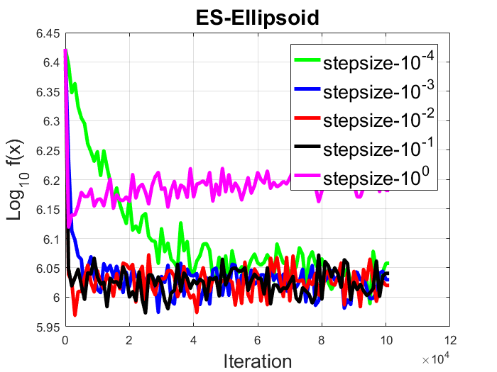
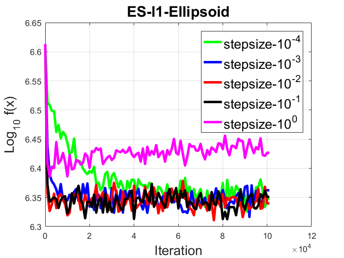
Refer to caption
(a) ES on Ellipsoid
Refer to caption
(b) ES on l1subscript๐‘™1l_{1} Ellipsoid
Refer to caption
(c) ES on l12subscript๐‘™12l_{\frac{1}{2}} Ellipsoid
Refer to caption
(d) ES on Discus
Refer to caption
(e) ES on Levy
Refer to caption
(f) ES on Rastrigin10
Figure 4: ES with different stepsize on different test functions
Refer to caption
(a) Reinforce GD on Ellipsoid
Refer to caption
(b) Reinforce GD on l1subscript๐‘™1l_{1} Ellipsoid
Refer to caption
(c) Reinforce GD on l12subscript๐‘™12l_{\frac{1}{2}} Ellipsoid
Refer to caption
(d) Reinforce GD on Discus
Refer to caption
(e) Reinforce GD on Levy
Refer to caption
(f) Reinforce GD on Rastrigin10
Figure 5: Standard Reinforce Gradient Descent with different stepsize on different test functions