Sparse Identification of Contrast Gain Control in the Fruit Fly Photoreceptor and Amacrine Cell Layer
Abstract
The fruit fly’s natural visual environment is often characterized by light intensities ranging across several orders of magnitude and by rapidly varying contrast across space and time. Fruit fly photoreceptors robustly transduce and, in conjunction with amacrine cells, process visual scenes and provide the resulting signal to downstream targets. Here we model the first step of visual processing in the photoreceptor-amacrine cell layer. We propose a novel divisive normalization processor (DNP) for modeling the computation taking place in the photoreceptor-amacrine cell layer. The DNP explicitly models the photoreceptor feedforward and temporal feedback processing paths and the spatio-temporal feedback path of the amacrine cells. We then formally characterize the contrast gain control of the DNP and provide sparse identification algorithms that can efficiently identify each the feedforward and feedback DNP components. The algorithms presented here are the first demonstration of tractable and robust identification of the components of a divisive normalization processor. The sparse identification algorithms can be readily employed in experimental settings, and their effectiveness is demonstrated with several examples.
1 Introduction
Sensory processing systems in the brain extract relevant information from inputs whose amplitude can vary orders of magnitude [1, 2, 3, 4]. Consequently, at each layer of processing, starting right from sensory transduction, neurons need to map their output into a range that can be effectively processed by subsequent neural circuits. As an example, photoreceptors [5, 6, 7, 8] and olfactory receptor neurons [9, 10] in both vertebrates and invertebrates, adapt to a large range of intensity/temporal contrast values of visual and odorant stimuli. Adaptation to mean and variance of the stimuli has been observed in the auditory system [11, 12] as well. Further down the visual pathway, motion sensitive neurons in vertebrates and invertebrates, have been shown to be robust at various brightness and contrast levels [13, 14, 15].
Early visual circuits such as the photoreceptor/amacrine cell layer of the fruit fly brain are believed to perform spatio-temporal intensity and contrast gain control for dynamic adaptation to visual stimuli whose intensity and contrast vary orders of magnitude both in space and time. However, current theoretical methods of describing spatio-temporal gain control lack a systematic framework for characterizing its dynamics and identification algorithms to estimate circuit components are currently not available.
Divisive normalization [16] has been proposed as a canonical circuit model of computation for many sensory processing circuits underlying adaptation and attention. However, there is a lack of general mathematical framework for identifying such computations from recorded data. In this paper we model the phoreceptor/amacrine cells layer of the fruit fly as a feedforward and feedback temporal and spatio-temporal divisive normalization processor. We provide efficient algorithms for identifying all the components of the temporal as well spatio-temporal divisive normalization processors.
This manuscript is organized as follows. In Section 2 the overall architecture of the divisive normalization processor (DNP) is introduced and its power of modeling contrast gain control demonstrated. We first describe in Section 2.1 the biological model of photoreceptor-amacrine cell layer. In Section 2.2, we introduce a general model for divisive normalization in the time domain. The temporal DNP consists of the ratio of two non-linear functionals acting on the input stimulus. In Section 2.3 we then extend the model to space-time domain to include models of lateral feedback from amacrine cells, and demonstrate its processing power. In Sections 3 and 4, we provide identification algorithms and show that the temporal and spatio-temporal DNPs can be efficiently identified. We demonstrate the effectiveness of the algorithms with several examples. We conclude the paper with a discussion in Section 5.
2 The Architecture of Divisive Normalization Processors
In section 2.1 we start by motivating the present work. We then introduce the architecture of divisive normalization processors in the time domain (section 2.2) and space-time domain (section 2.3). Finally, in Appendix A we provide examples that characterize the I/O mapping of the class of temporal and spatio-temporal divisive normalization processors previously described.
2.1 Modeling the Photoreceptors and Amacrine Cells Layer
In what follows, we anchor the model description around the photoreceptor-amacrine cell layer of the fruit fly. The fly retina consists of ommatidia, each of which hosts photoreceptors whose axons terminate in a secondary neuropil called lamina. There, they provide inputs to columnar Large Monopolar Cells (LMCs) that project to the third visual neuropil, and to amacrine cells [17]. Amacrine cells are interneurons that innervate axon terminals of multiple photoreceptors. The photoreceptors, in turn, receive lateral feedback from the amacrine cells as well as feedback from LMCs such as L2 neurons [18, 19, 20].
A circuit diagram of the photoreceptor-amacrine cell layer is shown in Figure 1. For the sake of clarity we assume here that an ommatidium consists of a single photoreceptor. It has been shown that the outputs of photoreceptors exhibit rapid gain control through both the phototransduction process and the interaction with such feedback loops [21, 22, 23, 24, 25].
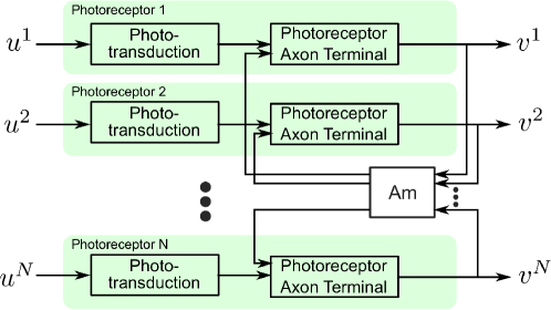
In what follows we propose a model comprising non-linear transformations combined with divisive normalization that can model such gain control and can account for diverse dynamics. We will also show that the model we propose can be systematically identified from observed input output pairs.
2.2 Divisive Normalization Processors in the Time Domain
In this section we present the modeling of temporal stimuli in 2.2.1 and introduce a class of temporal divisive normalization processors for modeling photoreceptors in section 2.2.2.
2.2.1 Modeling Temporal Stimuli
We model the temporal varying stimuli , , to be real-valued elements of the space of trigonometric polynomials [26]. The choice of the space of the trigonometric polynomials has, as we will see, substantial computational advantages. A temporal stimulus models the visual field arising at the input of a single photoreceptor.
Definition 1.
The space of trigonometric polynomials is the Hilbert space of complex-valued functions
| (1) |
over the domain , where
| (2) |
Here denotes the bandwidth, and the order of the space. Stimuli are extended to be periodic over with period .
is a Reproducing Kernel Hilbert Space (RKHS) [27] with reproducing kernel (RK)
| (3) |
We denote the dimension of by and .
Definition 2.
The tensor product space is an RKHS with reproducing kernel
| (4) |
Note that .
2.2.2 Temporal Divisive Normalization Processors
We first consider single photoreceptors without feedback from the amacrine cells shown in Figure 1. A schematic of the temporal divisive normalization processor (DNP) modeling the photoreceptor is shown in Figure 2. For notational simplicity, we consider a single photoreceptor here. The input visual stimulus to the photoreceptor is denoted by , and the output electric current by .
Remark 1.
Note that in a single photoreceptor, photons are first absorbed by a large number of microvilli [22] (not shown). Microvilli generate “quantum bumps” in response to photons; the photoreceptor aggregates the bumps and in the process creates the transduction current. Calcium ion influx and calcium diffusion into the photoreceptor cell body may change the sensitivity of the transduction cascade. A high concentration of calcium (buffer) can result in a photon to be ineffective and may also affect the duration and the magnitude of quantum bumps [28].

The DNP consists of 1) a feedforward Volterra Processor (VP) , 2) a feedforward normalization VP , and 3) a feedback normalization VP . The output of the photoreceptor amounts to
| (5) |
where
| (6) |
and
| (7) |
Here , are the zeroth-order Volterra kernels (constants), , are first-order Volterra kernels (impulse responses of linear filters), and , second-order Volterra kernels. As before, denotes the domain of the input space, and .
Remark 2.
2.2.3 Modeling Temporal DNP Feedback Filters
Definition 3.
Let , where denotes the space of Lebesgue integrable functions. The operator given by
| (8) |
is called the projection operator from to . Similarly, the operator given by
| (9) |
is called the projection operator from to .
Note, that for . Moreover, with . Thus,
| (10) |
and by assuming that , and we recover the simple form of equation (6).
We model the output waveforms , , to be real-valued elements of the space of trigonometric polynomials [26].
Definition 4.
The space of trigonometric polynomials is the Hilbert space of complex-valued functions
| (11) |
over the domain , where
| (12) |
Here denotes the bandwidth, and the order of the space. The output waveforms are extended to be periodic over with period .
is a Reproducing Kernel Hilbert Space (RKHS) [27] with reproducing kernel (RK)
| (13) |
We denote the dimension of by and .
Definition 5.
The tensor product space is an RKHS with reproducing kernel
| (14) |
Note that .
Definition 6.
Let , where denotes the space of Lebesgue integrable functions. The operator given by
| (15) |
is called the projection operator from to . Similarly, the operator given by
| (16) |
is called the projection operator from to .
We note that
| (17) |
If we now assume that and , and thereby and , respectively, and the above equation is identical with equation (7) above.
2.3 Divisive Normalization Processors in the Space-Time Domain
In Section 2.2, we described a temporal divisive normalization processor model. The normalization term was the sum of a processed version of the input and the output. However, many biological circuits are thought to exhibit lateral inhibition and gain control [30, 31, 32, 33, 16]. An example is provided by the photoreceptor-amacrine cell layer shown in Figure 1. In Figure 3, we provide a model of the schematic in Figure 1. This model is a ‘circuit’ extension of the one shown in Figure 2 and accounts explicitly for lateral inhibition. We anchor the extension in the visual system where the input domain is spatio-temporal.
In section 2.3.1 below we model spatio-temporal stimuli and in section 2.3.2 the spatio-temporal divisive normalization processors.
2.3.1 Modeling Spatio-Temporal Stimuli
In this section we provide a model of the interaction between a group of photoreceptors and an amacrine cell. In each photoreceptor, the phototransduction process converts light into current and excites the membrane of the photoreceptor. The voltage signal is then propagated through its axon to the lamina. While photoreceptors provide inputs to amacrine cells, their axon terminals also receive amacrine cell input. Since an amacrine cell innervates multiple lamina cartridges, it provides spatial feedback to several photoreceptors in a small neighborhood.
We extend the temporal divisive normalization processor depicted in Figure 2 to process spatio-temporal stimuli as shown in Figure 3. Each spatially sampled point, or pixel, denoted as , is first processed by a temporal DNP. For simplicity rather than picking different Volterra kernels for each branch, and are shared across branches. In addition, we introduce a Multi-Input Volterra Processor (MVP) to model the spatio-temporal feedback due to the amacrine cell. Each of the branches in Figure 3, without the input of the MVP block, is equivalent with the model in Figure 2.
2.3.2 Spatio-Temporal Divisive Normalization Processors
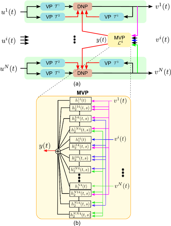
As shown in Figure 3(b), MVPs are comprised of second-order filters acting on DNP output pairs in addition to linear filters independently acting on each DNP output. Thus, the inputs to the MVP are the DNP outputs , and the MVP output amounts to
| (18) |
where
| (19) |
is the zerosth-order Volterra kernel (constant). Furthermore, , are the first-order Volterra kernels whose inputs are , respectively, and , are the second-order Volterra kernels whose inputs are the pairs , respectively.
The full model in Figure 3 thus consists of parallel channels as depicted in Figure 2 with the added cross-channel feedback normalization/gain control provided by the MVP block.
The overall output of the spatio-temporal DNP can be expressed as
| (20) |
W.L.O.G., we assume that .
2.3.3 Spatio-Temporal DNPs and Contrast Gain Control
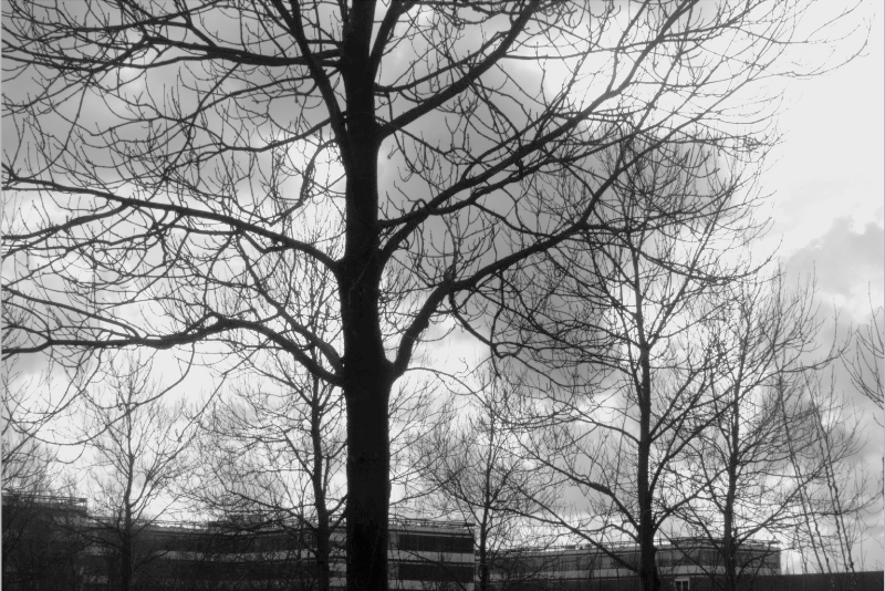
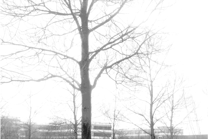
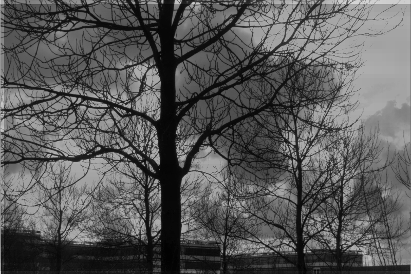
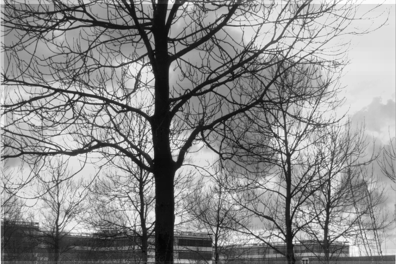
The relationship and some intuition behind the modeling power of spatio-temporal DNPs is provided in several examples Appendix A. The I/O of 3 simple spatio-temporal DNPs stimulated with different inputs is briefly mentioned here. In the first example, we evaluated the response of a DNP with 4 photoreceptors under different background light intensity levels. In Figure 8 one of the photoreceptors is subject to an additional flash of different light intensity, while the inputs of the other 3 are kept at the same background level. The steady state response of the photoreceptor that receives the additional flash is shifted as a function of the background-intensity level. In the second example, contrast gain control exerted by the amacrine cells is demonstrated for the same DNP in Figure 9. The effect of the MVP block on the RMS contrast can be clearly seen in Figure 9 and is quantitatively evaluated in Figure 10. Finally, an example of steady state I/O visualization of a natural image with resolution of pixels at low, medium and high luminance values is shown in Figure 11. The image was divided into spatio-temporal DNP blocks with a 4 pixel overlap in each direction.
3 Sparse Identification of Temporal DNPs
In what follows we derive sparse identification algorithms for the components of spatio-temporal DNPs depicted in Figure 2 and formally defined in equation (5). In what follows, we assume that during experimental trials, the single isolated photoreceptor is presented with test stimuli , and for each trial the outputs , are recorded. The objective is to identify the model components , from the knowledge of the inputs and outputs.
3.1 Deriving the Sparse Identification Algorithm for Temporal DNPs
Lemma 1.
With input stimuli presented to a temporal DNP, let the inputs and the outputs be sampled at times . Then,
| (21) |
where the sampling functions are given by
| (22) | ||||
and for all and .
Proof: See Appendix B.
Remark 3.
In order to solve the system of linear equations in (21) we rewrite them first in matrix form.
Lemma 2.
Eq. (21) can be expressed in matrix form as
| (23) |
for all , and , where denotes the trace operator, and
| Measurements | (24) | |||
| Unknowns | (27) | |||
| Sampling vectors | (30) |
Proof: See Appendix C for more notation and detailed proof.
A necessary condition on the number of trials and the number of measurements required for identifying the divisive normalization processor for solving the system of equations in Theorem 1 is that the number of trials and the number of total samples .
It is easy to see that solving the system of equations above suffers from the curse of dimensionality. As the dimension of increases, the number of samples needed to identify components increases quadratically. Note that the second-order Volterra kernels , have unique symmetric forms with orthogonal expansions as [29]
| (31) |
where , are orthogonal to each other. In what follows, we assume that the second-order Volterra kernels are sparse, i.e., for , where, . Sparse kernels often arise in modeling sensory processing, e.g., in complex cells in the primary visual cortex [35]. By exploiting the sparse structure of the second order kernels, the identification problem can be made tractable.
The sparsity of the kernels can be translated into a low-rank condition on the matrix representation of (see also Appendix C). Ideally, the optimization problem would be a rank minimization problem. But rank minimization being NP-hard, we use the surrogate of nuclear norm minimization instead, which is the convex envelope of the rank operator [36].
To perform sparse identification of the divisive normalization processor we devised Algorithm 1 below. By optimizing over and and subsequently assigning the corresponding block entries according to (27), Algorithm 1 identifies , and .
As a surrogate of rank minimization, Algorithm 1 minimizes a linear combination of the nuclear norm of , and the Euclidean norm of . The optimization constraints correspond i) in (33) to the generalized sampling problem allowing certain amount of error, ii) in (34) to zero mean slack variables, iii) in (35) to the zeros in the two blocks in the top-right of , iv) in (36) to the zeros in the block in the lower-left of , and v) in (37), (38) and (39), respectively, , and are Hermitian.
Algorithm 1.
and are the solution to the following optimization problem
| (32) | ||||
| s.t. | (33) | |||
| (34) | ||||
| (35) | ||||
| (36) | ||||
| (37) | ||||
| (38) | ||||
| (39) |
where denotes the nuclear norm defined as , are appropriately chosen hyperparameters, represent slack variables, represents a vector of all ones, represents a identity matrix, represents a matrix of all zeros, represents a matrix of all zeros and represents a matrix of all zeros with dimensions that makes the equation consistent.
Theorem 1.
The filters of the DNP are identified as and
| (40) | ||||
| (41) | ||||
| (42) |
where
| (43) |
Remark 4.
By exploiting the structure of low-rank second-order Volterra kernels, Algorithm 1 provides a tractable solution to the identification of the components of the divisive normalization processor.
3.2 Examples of Sparse Identification of Temporal DNPs
We provide here identification examples solved using Algorithm 1.
Example 1.
Here, we identify a temporal divisive normalization processor in Figure 2, where
We choose the input space to have . Thus , and . Note that all three second-order Volterra kernel exhibit low-rank structure. We presented the model with 25 stimuli from , whose coefficients were chosen to be i.i.d gaussian variables. Then, a total of measurements were used from the input and the observed output pairs to solve the identification problem using Algorithm 1. The results of the identification are shown in Figure 4. As can be seen from the figure, Algorithm 1 was able to identify the model with high precision using only measurements, much less than the measurements that would have been required to solve the generalized sampling problem directly. The factor of reduction in the required measurements is critical when the model needs to be identified in a much larger space, for example, a space of spatio-temporal stimuli as shown in the next example.
Example 2.
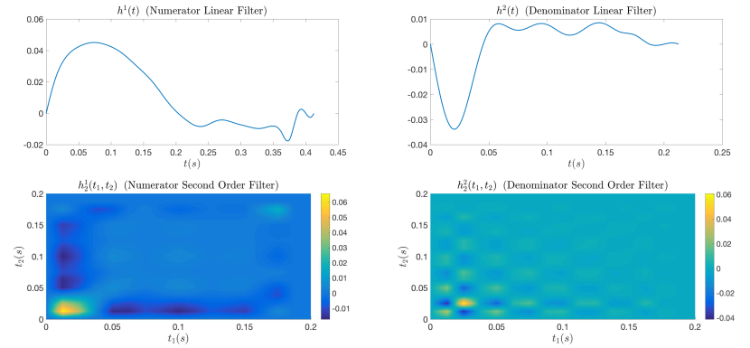
Here we identify a biophysical model of the drosophila photoreceptor. A detailed biophysical model of Drosophila photoreceptors was given in[5, 37]. The photoreceptor model consists of 30,000 microvilli. The photon absorption in each microvillus is described by a Poisson process whose rate is proportional to the number of photons per microvillus incident on the ommatidium. Photon absorption leads to a transduction process governed by a cascade of chemical reactions. The entire transduction process described by 13 successive differential equations and is given in [37]. The total number of equations of the photoreceptor model is .
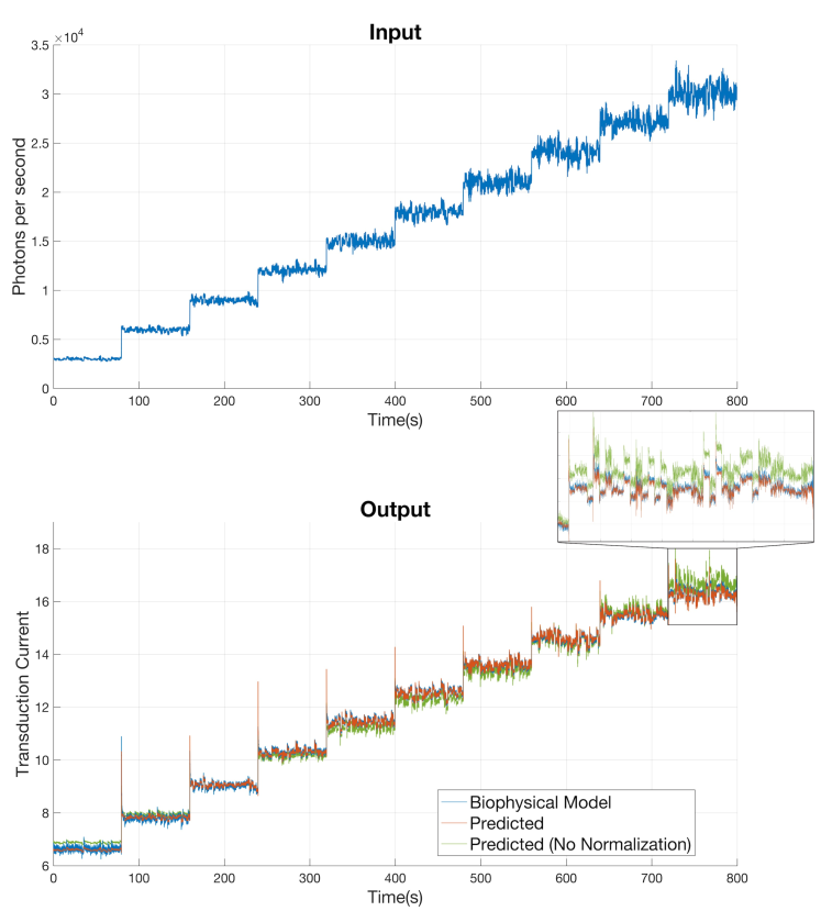
We presented the model mentioned above with a long stimulus consisting of random bandlimited fluctuations on top of different mean levels of light intensities. For each level, we used the first of the stimulus for identification and applied our identification framework on the resultant transduction current. The bandwidth of the input and output spaces was limited to Hz. The identified filters are depicted in Figure 5. We additionally trained a model without normalization (i.e., with only ); the outputs of the original biophysical model and the two identified models are shown in Figure 6. Without normalization, the identified model does not predict the output well across different light intensities. The SNR of the predicted output on training data for the normalization model was about , while the SNR of the predicted output on training data for the model without normalization was about .
4 Sparse Identification of Spatio-Temporal DNPs
In what follows we derive sparse identification algorithms for the components of spatio-temporal DNPs.
Given the spatio-temporal divisive normalization processor depicted in Fig. 3, we are interested in identifying all the filters from input and output observations. We formulate an optimization problem, which achieves such identification, with high fidelity and with a relatively small number of measurements.
4.1 Deriving the Sparse Identification Algorithm for Spatio-Temporal DNPs
Here, we make the assumption that the filters , and , , are followed by the LPF with bandwidth and that the output is sampled at a rate of , where is the maximum of the bandwidth of the filters and . By abuse of notation, we will use to denote the low-passed version of the actual output. Note that, based upon the assumptions on the bandlimited nature of the feedback filters acting on the output, the responses of these filters to the low-passed outputs will be the same as the responses to the actual outputs.
We present trials where input stimuli are chosen to be elements of the space of trigonometric polynomials for . We project the outputs on the Hilbert space of trigonometric polynomials , i.e., . Note that is approximately for large values of [38]. Further we assume that , the space of square integrable functions over domain and , the space of square integrable functions over domain .
We consider here the identification of the entire DNP circuit at once, for two reasons. First, as all channels are connected in the spatial domain through the MVP, the inputs to the MVP are the outputs of the entire DNP circuit. Therefore, all outputs are required to identify the MVP. Second, since , are shared across all channels, less trials are needed to identify these filters. We present the following
Lemma 3.
With trials presented to the spatio-temporal DNP, let the inputs and the outputs be sampled at times . Then, for , we have the following equations
| (44) | ||||
where the sampling functions are given by
| (45) | ||||
and for all , and .
Proof: See Appendix D.
Remark 5.
Theorem 3 suggests that identifying the lateral divisive normalization model is equivalent to solving a generalized sampling problem with noisy measurements. It also suggests that the output needs to be sampled at a high enough rate, and that the choice of the Hilbert space used to reconstruct the feedback filters is critical since incorrect choices for these parameters can negatively affect the identification by introducing ‘noise’ in the measurements.
We now present the following algorithm to identify the model that exploits the low-rank constraints imposed on the quadratic filters.
Lemma 4.
We provide the following algorithm to identify , , , , and .
Again, we assume that all the second-order filters have sparse structures akin to (31).
Algorithm 2.
Let and be the solution to the following optimization problem
| (56) | ||||
| (57) | ||||
| (58) | ||||
| (59) | ||||
| (60) | ||||
| (61) | ||||
| (62) | ||||
| (63) |
where are appropriately chosen hyperparameters and represent slack variables.
The constraints in Algorithm 2 are similar to those in Algorithm 1. Note that are not constrained to be Hermitian. This follows from the assumption that the MVP block may perform asymmetric processing on any pair of inputs to the block.
Theorem 2.
The identified spatio-temporal divisive normalization is specified as and
| (64) | ||||
| (65) | ||||
| (66) | ||||
| (67) | ||||
| (68) | ||||
| (69) |
where
| (70) |
and
| (71) |
Remark 6.
Assuming all the second-order kernels in the lateral divisive normalization model have rank , the expected number of measurements for Algorithm 2 to identify the model is of the order . When is large, the factor may become prohibitive in identifying the model. Additional assumptions on may help mitigate this and maintain tractability of solving the identification problem. For example, with the assumption that if and otherwise, the expected number of measurements required will .
4.2 An Example of Sparse Identification of a Spatio-Temporal DNP
We now present an example of identification obtained by Algorithm 2. We demonstrate here that, in addition to the identification of the Volterra kernels operating within each channel, the MVP in the spatio-temporal DNP can be identified.
Example 3.
Here, we choose the DNP in Fig. 3 with , and
| (72) |
| (73) |
| (74) |
| (75) |
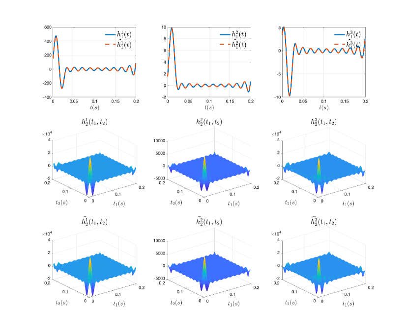
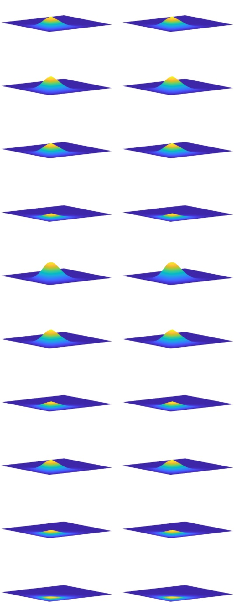
and the other Volterra kernels are set to 0. Note that Yiyin, and , are shared across all channels. In addition, in this case. We assumed knowledge of this symmetric structure of the model and adapted the identification algorithm accordingly and only identified 6 linear filters and 10 quadratic filters.


First-order Filters
Original
Identified
MVP Second-order Kernels
We performed the identification in the Hilbert space of bandlimited functions with and we chose the same space for the input stimuli and for both the feedforward and feedback filters. We solved for the filters truncated to a period of , and thus there were coefficients to be identified for the linear filters and coefficients to be identified for each of the quadratic filters. A total of measurements ( measurements from each cell) were used to perform the identification and the results are depicted in Figure 7. The average SNR of reconstruction across all filters was more than . Note that solving the generalized sampling problem directly for the same problem would have required at least measurements.
5 Discussion
As already mentioned in the introduction, the photoreceptor/amacrine cell layer of the early vision system of the fruit fly rapidly adapts to visual stimuli whose intensity and contrast vary orders of magnitude both in space and time.
In this paper we presented a spatio-temporal divisive normalization processor that models the transduction and the contrast gain control in the photoreceptor and amacrine cell layer of the fruit fly. It incorporates processing blocks that explicitly model the feedforword and the temporal feedback path of each photoreceptor and the spatio-temporal feedback from amacrine cells to photoreceptors. We demonstrated that with some simple choice of parameters, the DNP response maintains the contrast of the input visual field across a large range of average spatial luminance values.
We characterized the I/O of the spatio-temporal DNP and highlighted the highly nonlinear behavior of the DNP in contrast gain control. Despite the divisive nonlinearity, we provided an algorithm for the sparse identification of the entire DNP. We showed that the identification of the DNP can be interpreted as a generalized sampling problem. More importantly, the sparse identification algorithm does not suffer from the curse of dimensionality that would otherwise require a large number of measurements that is quadratically related to the dimension of the input and output spaces.
The DNP model opens a new avenue for exploring and quantifying the highly nonlinear nature of sensory processing. The DNP in Figure 3 can be further extended to allow the different transformations , to incorporate spatio-temporal Volterra kernels, thereby making it more versatile for modeling other types of sensory processing, including (i) interactions between cones and horizontal cells in vertebrate retinas [30], (ii) channels/glomeruli in olfactory circuits and interactions between them through local neurons [39, 9], and (iii) cross-suppression and gain control in the auditory [12, 40], and visual corticies [41, 42, 43].
Appendix A Spatio-Temporal DNPs and Contrast Gain Control
Here we characterize the I/O of simple DNPs stimulated with three different inputs. In the first example, we evaluate the response of a DNP under different background light intensity levels. In the second example, contrast gain control exerted by the amacrine cells is demonstrated with the same DNP. In the third example, a DNP consisting of DNPs tiling a visual field is stimulated with a natural image taken at low, medium and high luminance values. The DNP output is evaluated with and without the MVP block.
Example 4.
Here, we consider a simple DNP consisting of 4 photoreceptors and a single amacrine cell receiving inputs from and providing feedback to all 4 photoreceptors. The choices of the component filters of the DNP are as follows:
| (76) |
for the transformations and the kernels are:
| (77) |
| (78) |
for the transformation the kernels are,
| (79) |
| (80) |
and for the transformation the kernels are:
| (81) |
| (82) |
Here, the bandwidth of was chosen to be rad/s. The I/O of the fly’s individual photoreceptors in steady state is described by a saturating non-linearity similar in appearance to a sigmoid when plotted on a logarithmic scale [1]. Photoreceptors can deal with the orders of magnitude of the input stimuli while maintaining their output in a suitable range. In addition, the photoreceptors exhibit adaptation so that the sigmoidal curves shift to adjust to the mean local luminance value [16].
We examine here the steady state response of the above DNP under 4 different background light intensity levels. At the start of each trial, all 4 photoreceptors are first adapted to the same background light intensity level. One of the photoreceptors is then subject to an additional flash of different light intensity with a duration of 2 seconds, while the inputs to the other 3 are kept at the same background level. We observe the value of the steady state response of the photoreceptor that receives the additional flash. Figure 8 depicts the relationship between the observed steady state response and the light intensity of the flash, at the 4 background intensity levels. It demonstrates that the response of the DNP is background-dependent, and the overall slope and range are similar across different background levels. With the MVP block, the spatio-temporal DNP can reproduce responses of photoreceptors observed in experimental settings [16, 21].
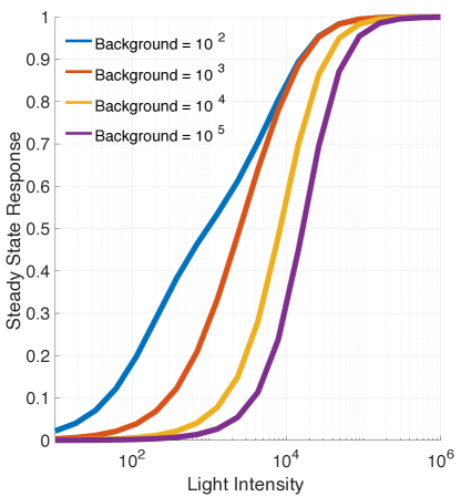
Since all the photoreceptors exhibit a sigmoid like non-linearity, the output of the retina will be constrained in a suitable current range that can be processed by postsynaptic neurons in the lamina. However, without adaptation to mean local luminance, the saturating nature of the non-linearities leads to a loss of spatial contrast. The spatial contrast is preserved by spatial gain control or adaptation modeled here with the MVP block.
Example 5.
Here, the I/O of DNPs with and without the MVP block is evaluated. Using the same DNP as in the example above, we stimulated the DNP with 25 “images” with a resolution of pixels. Each image has a different average luminance and root mean square (RMS) contrast. The RMS contrast is defined as the standard deviation of pixel intensities normalized by the mean i.e.,
| (83) |
where
| (84) |
and . These images are shown in the “input” block in Figure 9, with each bar represents the input intensity to one photoreceptor. Note that the pixels are extended along the y-axis for a quick visual examination.
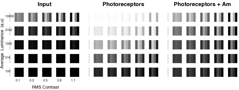
In the “Photoreceptors” block in Figure 9, the steady state responses of the DNP without the MVP block to the respective inputs are shown. Here pure black represents a response of 0 and white 1. This can be interpreted as a circuit in which the reciprocal connections between photoreceptors and amacrine cells are blocked.
In the “Photoreceptors Am” block in Figure 9, the steady state responses of the full DNP to their respective inputs are shown. Comparing the “Photoreceptors” and “Photoreceptors Am” block, the responses of the DNP without feedback are washed out, or exhibit low contrast, particularly at three of the four corners of the image array, i.e., when either the luminance or contrast is too high or too low. By contrast, the individual bars in the response of the full DNP model is more readily discernible across several orders of magnitude of luminance.
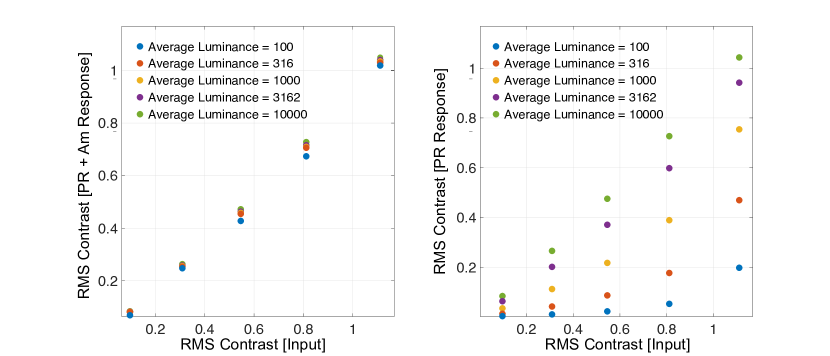
We note that a saturating non-linearity can maintain its output in a constrained range even when the input varies by orders of magnitude. However, the non-linearity may lead to a loss of spatial contrast. In contrast the DNP, constrains its output to a suitable range while maintaining the spatial contrast. This is demonstrated in Figure 10, where the RMS contrast of the input images in Figure 9 are plotted against the RMS contrasts of the responses for both cases - with and without MVP in the DNP. Spatial contrast, arguably, is an important feature of the image that should be preserved or even enhanced for subsequent stages of extraction of ethologically relevant information from the visual stimulus.
Example 6.
Here we apply a full-scale DNP model to a natural image. The image is taken in raw format so that its pixel values are proportional to the light intensity each pixel is exposed to [44]. The resolution of the image is . The image is first divided into blocks with a 4 pixel overlap in each direction. A DNP is assigned to each block, and the filters in the DNP are designed as follows:
| (85) |
for the transformations and the kernels are:
| (86) |
| (87) |
for the transformation the kernels are:
| (88) |
| (89) |
and for the transformation the kernels are:
| (90) |
| (91) |
where is the coordinate of pixel , and is the coordinate of the center pixel in the block. Here, the bandwidth of was chosen to be rad/s.
Input


Log(Input)

PhotoR
Response

PhotoR + Am
Response
Low Luminance
Medium Luminance
High Luminance
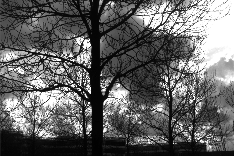
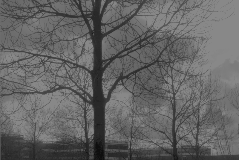
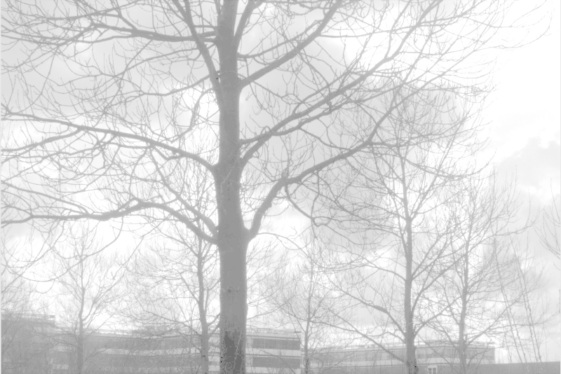
We tested the DNP using low, medium and high luminance (, , and ) of the original image measured in the number of photons and represented by arbitrary units. They are shown on the top row of Figure 11. The logarithm of the inputs are shown on the second row. On the third row, we show the response of the DNP without the MVP block, i.e., each photoreceptor processes independently a single pixel. The responses of the full DNP model are shown on the bottom row.
As can be seen from the Figure 11, the response of the DNP with MVP is robust across the different levels of luminance, showing the best quality for all three luminance levels. By contrast, the response of the DNP without MVP is either too dark for low contrast or saturated at high luminance. The contrast within each response is also significantly worse. It is also not ideal to use only a logarithmic nonlinearity to process the images (second row), as the contrast of the images is not sharp enough.
To conclude we note that, with a simple choice of filters, the spatio-temporal DNP proposed in section 2.3 operates in a range of luminance values spanning several orders of magnitude, much like the photoreceptor - amacrine cell layer. The contrast of the output of the DNP is not compromised while its range remains strongly bounded.
Appendix B Proof for Lemma 1
Appendix C Proof of Lemma 2
Let
| (94) |
| (95) |
| (96) |
and the vectors
| (97) |
the vector
| (98) |
the Hermitian matrices
| (99) |
| (100) |
and the Hermitian matrix
| (101) |
Further, let
| (102) |
where represents the coefficient of w.r.t basis element in such that , and represents conjugate transpose, and let
| (103) |
where represents the coefficient of w.r.t basis element in such that .
Finally, we define the vector
| (104) |
and matrix
| (105) |
Finally, we define the vector
| (106) |
and the matrix
| (107) |
The proof is based on two simple observations. First,
| (108) |
and therefore
Second,
| (109) | ||||
and, therefore,
| (110) |
Appendix D Proof of Lemma 3
For the trial, the output of the channel, by multiplying by the denominator of (20) with sampled at times we obtain
| (111) |
Finally with and the notation in (45), we get
| (112) |
and, therefore,
| (113) | ||||
for all , ,
and .
Appendix E Proof of Lemma 4
In addition to (94)-(101), let
| (114) |
| (115) |
and the vector
| (116) |
and the matrix
| (117) |
Note that are not necessarily Hermitian matrices. Further, by abuse of notation, let the vector
| (118) |
where represents the coefficient of w.r.t basis element in such that , and let the vector
| (119) |
where represents the coefficient of w.r.t basis element in such that .
Additionally, we define the vector
| (120) |
and the matrix
| (121) |
Finally, we define the vector
| (122) |
and the matrix
| (123) |
With the notation above, the proof follows the same steps as the proof of Lemma 2.
References
- [1] Simon B. Laughlin. Matching coding, circuits, cells, and molecules to signals: General principles of retinal design in the fly’s eye. Progress in Retinal and Eye Research, 13(1):165 – 196, 1994.
- [2] R. W. Rodieck. The First Steps in Seeing. Oxford University Press, 1998.
- [3] Marien de Bruyne, Peter J. Clyne, and John R. Carlson. Odor coding in a model olfactory organ: Thedrosophila maxillary palp. Journal of Neuroscience, 19(11):4520–4532, 1999.
- [4] Shawn R. Olsen, Vikas Bhandawat, and Rachel I. Wilson. Divisive normalization in olfactory population codes. Neuron, 66(2):287 – 299, 2010.
- [5] Zhuoyi Song, Marten Postma, Stephen Billings, Daniel Coca, Roger C. Hardie, and Mikko Juusola. Stochastic, adaptive sampling of information by microvilli in fly photoreceptors. Current Biology, 22:1371–1380, 2012.
- [6] Markus Meister and II Berry, Michael J. The neural code of the retina. Neuron, 22(3):435–450, 2018/08/15 1999.
- [7] Benjamin Scholl, Kenneth W Latimer, and Nicholas J Priebe. A retinal source of spatial contrast gain control. The Journal of neuroscience : the official journal of the Society for Neuroscience, 32(29):9824–9830, 07 2012.
- [8] Stephen A. Baccus and Markus Meister. Fast and slow contrast adaptation in retinal circuitry. Neuron, 36:909–919, 2002.
- [9] Rachel I. Wilson. Early olfactory processing in Drosophila: Mechanisms and principles. Annual Review of Neuroscience, 36:217–241, 2013.
- [10] Stuart Firestein. How the olfactory system makes sense of scents. Nature, 413:211 EP –, 09 2001.
- [11] Jan Clemens, Nofar Ozeri-Engelhard, and Mala Murthy. Fast intensity adaptation enhances the encoding of sound in drosophila. Nature Communications, 9:134, 2018.
- [12] Neil C Rabinowitz, Ben DB Willmore, Jan WH Schnupp, and Andrew J King. Contrast gain control in auditory cortex. Neuron, 70(6):1178–1191, 06 2011.
- [13] Adam Kohn and J Anthony Movshon. Neuronal adaptation to visual motion in area mt of the macaque. Neuron, 39(4):681–691, Aug 2003.
- [14] Diana Rien, Roland Kern, and Rafael Kurtz. Octopaminergic modulation of contrast gain adaptation in fly visual motion-sensitive neurons. Eur J Neurosci, 36(8):3030–3039, Oct 2012.
- [15] Hilary W Heuer and Kenneth H Britten. Contrast dependence of response normalization in area mt of the rhesus macaque. J Neurophysiol, 88(6):3398–3408, Dec 2002.
- [16] Matteo Carandini and David J. Heeger. Normalization as a canonical neural computation. Nature Reviews Neuroscience, 13:51–62, 2012.
- [17] K.-F. Fischbach and A. P. M. Dittrich. The optic lobe of Drosophila melanogaster. I. A Golgi analysis of wild-type structure. Cell and Tissue Research, 258:441–475, 1989.
- [18] Anton Nikolaev, Lei Zheng, Trevor J. Wardill, Cahir J. O’Kane, Gonzalo G. de Polavieja, and Mikko Juusola. Network adaptation improves temporal representation of naturalistic stimuli in drosophila eye: Ii mechanisms. PLOS ONE, 4(1):1–12, 01 2009.
- [19] Marta Rivera-Alba, Shiv N. Vitaladevuni, Yuriy Mishchenko, Zhiyuan Lu, Shin-ya Takemura, Lou Scheffer, Ian A. Meinertzhagen, Dmitri B. Chklovskii, and Gonzalo G. de Polavieja. Wiring Economy and Volume Exclusion Determine Neuronal Placement in the Drosophila Brain. Current Biology, 21(23):2000–2005, December 2011.
- [20] Peter Sterling and Simon Laughlin. Principles of Neural Design. The MIT Press, Cambridge, 2015.
- [21] T. Matić and S. B. Laughlin. Changes in the intensity-response function of an insect’s photoreceptors due to light adaptation. Journal of comparative physiology, 145(2):169–177, Jun 1981.
- [22] Mikko Juusola and Roger C. Hardie. Light adaptation in Drosophila photoreceptors: I. response dynamics and signaling efficiency at C. Journal of General Physiology, 117:3–25, 2001.
- [23] Lei Zheng, Gonzalo G. de Polavieja, Verena Wolfram, Musa H. Asyali, Roger C. Hardie, and Mikko Juusola. Feedback network controls photoreceptor output at the layer of first visual synapses in drosophila. The Journal of General Physiology, 127(5):495–510, 2006.
- [24] Simon B. Laughlin. Fly optic lamina as a guide to neural circuit design. In Gordon M. Shepard and Sten Grillner, editors, Handbook of brain microcircuits. Oxford University Press, 2nd edition, 2017.
- [25] Uwe Friederich, Stephen A. Billings, Roger C. Hardie, Mikko Juusola, and Daniel Coca. Fly photoreceptors encode phase congruency. PLOS ONE, 11(6):1–21, 06 2016.
- [26] Aurel A. Lazar, Eftychios A. Pnevmatikakis, and Yiyin Zhou. Encoding natural scenes with neural circuits with random thresholds. Vision Research, 50(22):2200–2212, October 2010. Special Issue on Mathematical Models of Visual Coding.
- [27] Alain Berlinet and Christine Thomas-Agnan. Reproducing Kernel Hilbert Spaces in Probability and Statistics. Kluwer Academic Publishers, 2004.
- [28] Alain Pumir, Jennifer Graves, Rama Ranganathan, and Boris I. Shraiman. Systems analysis of the single photon response in invertebrate photoreceptors. Proceedings of the National Academy of Sciences, 105(30):10354–10359, 2008.
- [29] Wilson J. Rugh. Nonlinear System Theory: Volterra/Wiener Approach. Johns Hopkins University Press, Baltimore, MD, 1981.
- [30] Marjelle VanLeeuwen, Iris Fahrenfort, Trijntje Sjoerdsma, Robert Numan, and Maarten Kamermans. Lateral gain control in the outer retina leads to potentiation of center responses of retinal neurons. Journal of Neuroscience, 29(19):6358–6366, 2009.
- [31] Colin Blakemore, Roger H. S. Carpenter, and Mark A. Georgeson. Lateral inhibition between orientation detectors in the human visual system. Nature, 228:37–39, 1970.
- [32] Shawn R Olsen and Rachel I Wilson. Lateral presynaptic inhibition mediates gain control in an olfactory circuit. Nature, 452(7190):956–960, 04 2008.
- [33] Uri Polat and Dov Sagi. Lateral interactions between spatial channels: Suppression and facilitation revealed by lateral masking experiments. Vision Research, 33(7):993–999, 1993.
- [34] Ole Christensen. Frames and Bases: An Introductory Course. Birkhäuser, 2008.
- [35] Aurel A Lazar, Nikul H Ukani, and Yiyin Zhou. Sparse functional identification of complex cells from spike times and the decoding of visual stimuli. The Journal of Mathematical Neuroscience, 8(1):2, 2018.
- [36] M. Fazel, H. Hindi, and S. Boyd. Rank minimization and applications in system theory. In Proceedings American Control Conference, pages 3273–3278, June 2004.
- [37] Aurel A. Lazar, Konstantinos Psychas, Nikul H. Ukani, and Yiyin Zhou. A Parallel Processing Model of the Drosophila Retina. Neurokernel Request for Comments, Neurokernel RFC #3, August 2015. http://dx.doi.org/10.5281/zenodo.30036.
- [38] Robert Martin. Approximation of Omega-bandlimited functions by Omega-bandlimited trigonometric polynomials, volume 6. 09 2007.
- [39] A. A. Lazar and C.-H. Yeh. A parallel processing model of drosophila olfactory sensory neurons and its biological validation. Neurokernel Request for Comments. Neurokernel RFC #10, Dec 2017.
- [40] Ryan G. Natan, Isaac M. Carruthers, Laetitia Mwilambwe-Tshilobo, and Maria N. Geffen. Gain control in the auditory cortex evoked by changing temporal correlation of sounds. Cerebral Cortex, 27(3):2385–2402, 2017.
- [41] John D. Allison, Kevin R. Smith, and A.B. Bonds. Temporal-frequency tuning of cross-orientation suppression in the cat striate cortex. Visual Neuroscience, 18(6):941–948, 2001.
- [42] Wilson S. Geisler and Duane G. Albrecht. Cortical neurons: Isolation of contrast gain control. Vision Research, 32(8):1409–1410, 1992.
- [43] Nicholas J Priebe and David Ferster. Mechanisms underlying cross-orientation suppression in cat visual cortex. Nature Neuroscience, 9:552 EP –, 03 2006.
- [44] J. H. van Hateren and A. van der Schaaf. Independent component filters of natural images compared with simple cells in primary visual cortex. Proceedings of the Royal Society of London. Series B: Biological Sciences, 265(1394):359–366, Mar 1998.