Optimal Performance of a Three-level Quantum Refrigerator

Abstract

We study the optimal performance of a three-level quantum refrigerator using two different objective functions: cooling power and $\chi$-function. For both cases, we obtain general expressions for the coefficient of performance (COP) and derive its well-known lower and upper bounds for the limiting cases when the ratio of system-bath coupling constants at the hot and cold contacts approaches infinity and zero, respectively. We also show that the cooling power is optimizable only in the local region with respect to one control frequency, while $\chi$-function can be optimized globally with respect to two control frequencies. Additionally, we show that in the low-temperatures regime, our model of refrigerator can be mapped to Feynman’s ratchet and pawl model, a classical mesoscopic heat engine. In the parameter regime where both cooling power and $\chi$-function can be optimized, we compare the cooling power of the quantum refrigerator at maximum $\chi$-function with the optimum cooling power.

I Introduction

In 1824, Carnot discovered that the efficiency of any heat engine operating between two reservoirs at temperatures $T_{h}$ and $T_{c}$ ($T_{c}<T_{h}$), is bounded from above by the Carnot efficiency, $\eta_{\rm C}=1-T_{c}/T_{h}$. If a heat cycle is reversed—turning it into a refrigerator—the corresponding measure, called the coefficient of performance (COP), is similarly bounded from above by $\epsilon_{\rm C}=T_{c}/(T_{h}-T_{c})$. Somehow, the optimization analysis of irreversible refrigerators Yan and Chen (1990); Agrawal and Menon (1990); Allahverdyan et al. (2010); Apertet et al. (2013) turns out to be more involved than that of heat engines. For instance, power output is a reasonable objective to optimize for a heat engine. Under the assumptions of endoreversibility and Newton’s law for heat transfer, the efficiency at maximum power was derived by Curzon-Ahlborn (CA) Curzon and Ahlborn (1975):

$$\eta_{\rm CA}=1-\sqrt{1-\eta_{C}}.$$ (1)

Then, Esposito and coauthors Esposito et al. (2010) introduced the concept of a low-dissipation heat engine and obtained lower and upper bounds on the efficiency at maximum power. Further, for the symmetric dissipation at the hot and the cold contacts, they reproduced CA value. Izumida and Okuda Izumida, Y. and Okuda, K. (2012) showed that results of low-dissipation model can be obtained in the optimization of minimally non-linear irreversible heat engines. CA-efficiency is also obtained using inference in models of limited information based on Jeffreys prior probability function Johal (2010); Thomas and Johal (2015). Recently, in a global approach to irreversible entropy generation Johal (2018) which is independent of the specific nature of heat cycle, CA-efficiency was related to geometric mean value of the heat exchanged with reservoirs.

On the other hand, it is not possible to optimize directly the cooling power (CP) of endoreversible and low-dissipation refrigerators in general by taking the same assumptions useful for the optimization of a corresponding model of heat engine. An expression analogous to CA efficiency was first obtained for refrigerators by Yan and Chen Yan and Chen (1990) by maximizing a new criterion, $\chi=\epsilon\dot{Q}_{c}$, which represents a trade-off between the COP ($\epsilon$) and CP ($\dot{Q}_{c}$) of the refrigerator. The COP at optimal $\chi$ is given by

$$\epsilon_{\rm CA}=\sqrt{1+\epsilon_{\rm C}}-1,$$ (2)

which also holds for many models of classical de Tomás et al. (2012); Izumida et al. (2013); Velasco et al. (1997); Thomas and Johal (2015); Johal (2018, 2019) and quantum refrigerators Allahverdyan et al. (2010); Abah and Lutz (2016).

Agrawal and Menon Agrawal and Menon (1990) showed that CP of endoreversible refrigerators becomes optimizable if we take into account the time spent on adiabatic branches. However, this results in a model-dependent expression for the COP. Similarly, CP of a classical endoreversible refrigerator can be optimized by considering non-Newtonian laws of heat transfer, employed earlier to optimize the power output in CA model Yan and Chen (1990). Again, this results in non-universal formulae for the COP of the refrigerator that depend on phenomenological heat conductivities. Recently, carrying the research in optimization of refrigerators one step forward, Correa et al. maximized the CP of a quantum endoreversible refrigerator in high-temperature regime and obtained model-independent expression for the COP Correa et al. (2014a).

In this work, we study the optimal performance of a three-level quantum refrigerator Scovil and Schulz-DuBois (1959); Geusic et al. (1959). It is regarded that the study of three level systems pioneered by Scovil and Schulz-DuBois (SSD), started the field of quantum thermodynamics Kosloff (2013); Mahler (2014); Vinjanampathy and Anders (2016); Millen and Xuereb (2016); Deffner and Campbell (2019); Alicki and Kosloff (2018); Binder et al. (2018). In recent years, these systems have also been employed to study quantum heat engines (refrigerators) Geva and Kosloff (1994, 1996); Kosloff and Levy (2014); Dorfman et al. (2018); Singh and Johal (2019); Jaseem et al. (2018); Klatzow et al. (2019) and quantum absorption refrigerators Linden et al. (2010); Levy and Kosloff (2012); Correa et al. (2013); Agarwalla et al. (2017); Kilgour and Segal (2018); Holubec and Novotný (2019); Maslennikov et al. (2019); Mitchison et al. (2016); Brask and Brunner (2015). Our choice of the model is motivated by the observation that it can be optimized for both CP and $\chi$-function and yields model-independent expressions for lower and upper bounds on the COP in each case.

The paper is organized as follows. In Sec.II, we discuss the model of SSD refrigerator. In Sec. III, we optimize the CP of the refrigerator and obtain the general expression for the optimal COP, and find lower and upper bounds on the COP. In Sec. IV, we optimize the $\chi$-function and obtain analytic expressions for the COP for global as well as local optimization scheme. We conclude in Sec. V.

II Model of Three-Level Quantum Refrigerator

The model consists of a three-level atomic system continuously coupled to two thermal reservoirs and to a single mode of classical electromagnetic field as shown in Fig. 1. In refrigerators, heat is extracted from the cold reservoir and dumped into the hot reservoir, with the help of an external agency. The power input mechanism is modeled by an external single mode field coupled to the levels $|0\rangle$ and $|1\rangle$, inducing transitions between these levels. The population in level $|1\rangle$ then relaxes to level $|g\rangle$ by rejecting heat to the hot bath. The system then jumps from level $|g\rangle$ to level $|1\rangle$ by absorbing energy from the cold bath.

Figure 1: (Color online) Schematic of three-level laser refrigerator continuously coupled to two heat reservoirs at temperatures $T_{c}$ and $T_{h}$ with coupling constants $\Gamma_{c}$ and $\Gamma_{h}$ respectively. A single-mode classical field drives the transition between levels $|0\rangle$ and $|1\rangle$, and $\lambda$ represents the strength of matter-field coupling.

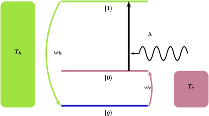
The Hamiltonian of the system is given by: $H_{0}=\hbar\sum\omega_{k}|k\rangle\langle k|$, where the summation runs over all three states and $\omega_{k}$ represents the relevant atomic frequency. The interaction with the single mode lasing field of frequency $\omega$, under the rotating wave approximation, is described by the semiclassical hamiltonian: $V(t)=\hbar\lambda(e^{i\omega t}|1\rangle\langle 0|+e^{-i\omega t}|0\rangle\langle 1|)$, where $\lambda$ is the field-matter coupling constant. The most general time-independent dissipator generating a completely positive, trace-preserving and linear evolution was derived by Gorini, Kossakowski and Sudarshan Gorini et al. (1976), and Lindblad Lindblad (1976). The time evolution of the system is described by the following master equation:

$$\dot{\rho}=-\frac{i}{\hbar}[H_{0}+V(t),\rho]+\mathcal{L}_{h}[\rho]+\mathcal{L}_{c}[\rho],$$ (3)

where $\mathcal{L}_{h(c)}[\rho]$ represents the dissipative Lindblad superoperator describing the system-bath interaction with the hot (cold) reservoir:

$$\mathcal{L}_{h}[\rho] = \Gamma_{h}(n_{h}+1)(2|g\rangle\langle g|\rho_{11}-|1\rangle\langle 1|\rho-\rho|1\rangle\langle 1|)$$ (4)

$$+\Gamma_{h}n_{h}(2|1\rangle\langle 1|\rho_{gg}-|g\rangle\langle g|\rho-\rho|g\rangle\langle g|),$$

$$\mathcal{L}_{c}[\rho] = \Gamma_{c}(n_{c}+1)(2|g\rangle\langle g|\rho_{00}-|0\rangle\langle 0|\rho-\rho|0\rangle\langle 0|)$$ (5)

$$+\Gamma_{c}n_{c}(2|0\rangle\langle 0|\rho_{gg}-|g\rangle\langle g|\rho-\rho|g\rangle\langle g|).$$

Here $\Gamma_{h}$ and $\Gamma_{c}$ are the Weisskopf-Wigner decay constants, and $n_{h(c)}=1/(\exp[\hbar\omega_{h(c)}/k_{\rm B}T_{h(c)}]-1)$ is the average occupation number of photons in hot (cold) reservoir satisfying the relations $\omega_{c}=\omega_{0}-\omega_{g}$, $\omega_{h}=\omega_{1}-\omega_{g}$.

For our model, it is possible to find a rotating frame in which the steady-state density matrix $\rho_{R}$ is time independent [10]. Defining $\bar{H}=\hbar(\omega_{g}|g\rangle\langle g|+\frac{\omega}{2}|1\rangle\langle 1|-\frac{\omega}{2}|0\rangle\langle 0|)$, an arbitrary operator $A$ in the rotating frame is given by $A_{R}=e^{i\bar{H}t/\hbar}Ae^{-i\bar{H}t/\hbar}$. It can be seen that $\mathcal{L}_{h}[\rho]$ and $\mathcal{L}_{c}[\rho]$ remain unchanged under this transformation. The time evolution of the system density matrix in the rotating frame can be written as

$$\dot{\rho_{R}}=-\frac{i}{\hbar}[H_{0}-\bar{H}+V_{R},\rho_{R}]+\mathcal{L}_{h}[\rho_{R}]+\mathcal{L}_{c}[\rho_{R}]$$ (6)

where $V_{R}=\hbar\lambda(|1\rangle\langle 0|+|0\rangle\langle 1|)$.

In a series of papers Boukobza and Tannor (2006a, b, 2007), Boukobza and Tannor formulated a new way of quantifying heat and work for a weak system-bath coupling Alicki (1979). Then, the input power and heat flux of the refrigerator are defined as follows:

$$P = \frac{i}{\hbar}{\rm Tr}([H_{0},V_{R}]\rho_{R}),$$ (7)

$$\dot{Q_{c}} = {\rm Tr}(\mathcal{L}_{c}[\rho_{R}]H_{0}),$$ (8)

Calculating the traces (see Appendix A) appearing in right hand side of the Eqs. (7) and (8), the power and heat flux can be written as:

$$P=i\hbar\lambda(\omega_{h}-\omega_{c})(\rho_{01}-\rho_{10}),$$ (9)

$$\dot{Q_{c}}=i\hbar\lambda\omega_{c}(\rho_{10}-\rho_{01}),$$ (10)

where $\rho_{01}=\langle 0|\rho_{R}|1\rangle$ and $\rho_{10}=\langle 1|\rho_{R}|0\rangle$. Then, the COP is given by

$$\epsilon=\frac{\dot{Q}_{c}}{P}=\frac{\omega_{c}}{\omega_{h}-\omega_{c}},$$ (11)

which satisfies $\epsilon\leq\epsilon_{\rm C}$.

III Optimization Of Cooling Power

Figure 2: (Color online) 3D-plot of CP [Eq. (41)] in terms of control frequencies $\omega_{c}$ and $\omega_{h}$ for $\hbar=1,k_{\rm B}=1,\Gamma_{h}=3.4,\Gamma_{c}=3.2,\lambda=3,T_{h}=60,T_{c}=40$.

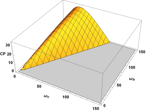
In this section, we optimize CP of the refrigerator and obtain the expression for the corresponding COP. The general expression for CP is derived in Appendix A, see Eq. (41). We show the 3D-plot of CP with respect to $\omega_{c}$ and $\omega_{h}$ in Fig. 2. It is clear from the figure that a well defined local maximum on $\omega_{c}$ exists whereas there is no such local maximum on $\omega_{h}$. In other words, CP is optimizable with respect to $\omega_{c}$ only. We have played with a wide range of different values of the concerned parameters ($\Gamma_{c,h},T_{c,h},\lambda$), but the basic trend of the graph remains the same and it does not change the main result. However, in this case, an analytic expression for the COP seems hard to obtain.

In order to derive the COP in a closed form, we work in the high-temperatures regime Kosloff (1984); Geva and Kosloff (1992); Abah et al. (2012); Correa et al. (2013, 2014b) and assume that the matter-field coupling is very strong compared to the system-bath coupling ($\lambda\gg\Gamma_{c,h}$) Dorfman et al. (2018). In this regime, it is possible to obtain model-independent performance benchmarks for both quantum engines and refrigerators Abah et al. (2012); Uzdin and Kosloff (2014); Correa et al. (2014a); Geva and Kosloff (1992). Then, we can approximate $n_{h}\simeq k_{\rm B}T_{h}/\hbar\omega_{h}$ and $n_{c}\simeq k_{\rm B}T_{c}/\hbar\omega_{c}$ and the expression for CP is simplified to be:

$$\dot{Q_{c}}=2\hbar\Gamma_{h}\frac{\omega_{c}(\tau\omega_{h}-\omega_{c})}{\tau\omega_{h}+\gamma\omega_{c}},$$ (12)

where $\gamma=\Gamma_{h}/\Gamma_{c}$ and $\tau=T_{c}/T_{h}\equiv\epsilon_{\rm C}/(1+\epsilon_{\rm C})$. One can optimize $\dot{Q}_{c}$ in Eq. (12) within a local region at fixed $\omega_{h}$ by setting $\partial\dot{Q}_{c}/\partial\omega_{c}=0$, which leads to the optimal solution:

$$\omega_{c}^{*}=\omega_{h}\frac{(\sqrt{1+\gamma}-1)\tau}{\gamma},$$ (13)

yielding the following form of the COP at maximum CP

$$\epsilon^{*}=\frac{\epsilon_{\rm C}}{1+\sqrt{1+\gamma}(1+\epsilon_{\rm C})}.$$ (14)

We note that $\epsilon^{*}$ is a monotonically decreasing function of $\gamma$. Therefore, we can obtain lower and upper bounds on the COP at maximum CP by letting $\gamma\rightarrow\infty$ and $\gamma\rightarrow\ 0$, respectively:

$$0\leq\epsilon^{*}\leq\frac{\epsilon_{\rm C}}{2+\epsilon_{\rm C}}.$$ (15)

The above bounds can be obtained in a variety of other models Izumida et al. (2015); Apertet et al. (2013) and approaches Johal (2018, 2019). In particular, the upper bound above is also obtained for an endoreversible quantum refrigerator (see Eq. (14) in Ref. Correa et al. (2014a) for $d_{c}=1$) operating at maximum CP. The reason behind this is that like Ref. Correa et al. (2014a), we also consider here the unstructured bosonic baths with a flat spectral density in one-dimension ($d_{c}=1$).

Similarly, substituting Eq. (13) in Eq. (12,) the optimal CP is given by:

$${\dot{Q}_{c}}^{*}=2\hbar\Gamma_{h}\omega_{h}\frac{(2+\gamma-2\sqrt{1+\gamma})\epsilon_{\rm C}}{(1+\epsilon_{\rm C})\gamma^{2}}.$$ (16)

For future reference, we find the expressions for ${\dot{Q}_{c}}^{*}$ in the limiting cases $\gamma\rightarrow 0$ and $\gamma\rightarrow\infty$:

$${\dot{Q}_{c(\gamma\rightarrow 0)}}^{*} = \frac{\hbar\Gamma_{h}\omega_{h}}{2}\frac{\epsilon_{\rm C}}{1+\epsilon_{\rm C}},$$ (17)

$${\dot{Q}_{c(\gamma\rightarrow\infty)}}^{*} = 2\hbar\Gamma_{c}\omega_{h}\frac{\epsilon_{\rm C}}{1+\epsilon_{\rm C}}.$$ (18)

IV Optimization Of $\chi$-Function

The $\chi$-function, $\chi=\epsilon\dot{Q}_{c}$ has already been shown to be a suitable figure of merit in the study of optimal performance of classical de Tomás et al. (2012); Izumida et al. (2013) as well as quantum refrigerators Allahverdyan et al. (2010); Yuan et al. (2014); Abah and Lutz (2016). In the following, we reaffirm this observation by pointing out that in the case of SSD refrigerator, it is possible to globally optimize the $\chi$-function with respect to control frequencies $\omega_{c}$ and $\omega_{h}$. This presents the advantage of optimizing $\chi$-function over CP which can only be optimized in a local region.

IV.1 Global Optimization

In the general case, again it is not possible to obtain analytic expression for the COP. Therefore, we optimize Eq. (A12) numerically and present our results in Table I.

Table 1: COP at global optimization of $\chi$-function. Here $T_{c}=50,T_{h}=100$. The results shown in first, second and third rows correspond to $\Gamma_{h}=1,\Gamma_{c}=2000;\Gamma_{h}=1,\Gamma_{c}=1$; and $\Gamma_{h}=2000,\Gamma_{c}=1$, respectively. For the given values of $T_{c}$ and $T_{h}$, $\epsilon_{\rm CA}$ = 0.414213.

	$\lambda=1$	$\lambda=100$	$\lambda=10000$
$\gamma=0.0005$	$\epsilon=0.459333$	$\epsilon=0.475244$	$\epsilon=0.476904$
$\gamma=1$	$\epsilon=0.441015$	$\epsilon=0.43729$	$\epsilon=0.437283$
$\gamma=2000$	$\epsilon=0.42461$	$\epsilon=0.372163$	$\epsilon=0.346034$

Low-temperatures regime

The low-temperatures regime is governed by the condition: $k_{\rm B}T_{c,h}\ll\hbar\omega_{c,h}$, such that $n_{c,h}\approx e^{-\hbar\omega_{c,h}/k_{\rm B}T_{c,h}}\ll 1$. Simplifying Eq. (A12), we get the expression for $\chi$-function as follows

$$\chi=\frac{2\hbar\lambda^{2}\Gamma_{c}\Gamma_{h}(n_{c}-n_{h})\omega_{c}^{2}}{(\Gamma_{c}+\Gamma_{h})(\lambda^{2}+\Gamma_{c}\Gamma_{h})(\omega_{h}-\omega_{c})}.$$ (19)

Optimization of Eq. (19), with respect to $\omega_{h}$ and $\omega_{c}$, yields the following equations:

$$e^{\hbar\omega_{h}/k_{\rm B}T_{h}-\hbar\omega_{c}/k_{\rm B}T_{c}} = 1+\frac{\hbar\omega_{c}\epsilon_{\rm C}}{k_{\rm B}T_{c}\epsilon(1+\epsilon_{\rm C})},$$ (20)

$$e^{\hbar\omega_{h}/k_{\rm B}T_{h}-\hbar\omega_{c}/k_{\rm B}T_{c}} = \frac{k_{\rm B}T_{c}(2+\epsilon)}{k_{\rm B}T_{c}(2+\epsilon)-\hbar\omega_{c}}.$$ (21)

The above equations cannot be solved analytically for $\omega_{h}$ and $\omega_{c}$. However, they can be combined to give the following transcendental equation:

$$\frac{(\epsilon_{\rm C}-\epsilon)(2\epsilon_{\rm C}-\epsilon)}{\epsilon\epsilon_{\rm C}(1+\epsilon_{\rm C})}=\ln\left[\frac{(2+\epsilon)\epsilon_{\rm C}}{\epsilon(1+\epsilon_{\rm C})}\right],$$ (22)

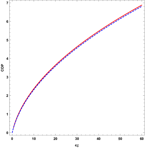
which clearly indicates that COP at maximum $\chi$-function depends upon $\epsilon_{\rm C}$ only and is independent of system parameters. Eq. (22) along with the expression, $\epsilon_{\rm CA}=\sqrt{1+\epsilon_{\rm C}}-1$, is plotted in Fig. 3, from which it is clear that COP of the SSD refrigerator operating in low-temperatures regime is higher than, though quite close to $\epsilon_{\rm CA}$. See also Appendix D for the mapping of the refrigerator model in the above regime to Feynman’s ratchet and pawl model.

Figure 3: (Color online) Plot of the COP versus $\epsilon_{\rm C}$. Solid red curve represents Eq. (22) and dashed blue curve represents the equation $\epsilon_{\rm CA}=\sqrt{1+\epsilon_{\rm C}}-1$.

IV.2 Local optimization in high-temperatures regime

High temperatures along with a strong matter-field coupling is another operational regime in which we can obtain model-independent benchmarks from the optimization of $\chi$-function. In this regime, the expression for $\chi$ is simplified to:

$$\chi=\epsilon\dot{Q_{c}}=\frac{2\hbar\Gamma_{h}\omega_{c}^{2}(\tau\omega_{h}-\omega_{c})}{(\tau\omega_{h}+\gamma\omega_{c})(\omega_{h}-\omega_{c})}.$$ (23)

If we attempt a two-parameter optimization by setting $\partial\chi/\partial\omega_{c}=0$ and $\partial\chi/\partial\omega_{h}=0$, it gives the trivial solution, $\omega_{h}=\omega_{c}=0$. Although in the previous section, we have shown the existence of global maximum of $\chi$ under general conditions, no such global maximum exists in this regime. It indicates that the assumption of high temperatures might not be justified for the simultaneous optimization with respect to $\omega_{c}$ and $\omega_{h}$. Since two-parameter optimization fails, we optimize $\chi$-function alternately with respect to $\omega_{h}$ ($\omega_{c}$ fixed) and $\omega_{c}$ ($\omega_{h}$ fixed). For fixed $\omega_{c}$, setting $\partial\chi/\partial\omega_{h}=0$, we obtain

$$\omega_{h}=\omega_{c}\frac{\gamma-\tau(1+\gamma)}{\tau\big{(}1-\sqrt{(1+\gamma)(1-\tau)}\big{)}}.$$ (24)

Substituting in Eq. (11), and writing in terms of Carnot COP $\epsilon_{\rm C}$, we get the following form of COP at maximum $\chi$-function:

$$\epsilon^{*}=\frac{\epsilon_{\rm C}}{1+\sqrt{(1+\gamma)(1+\epsilon_{\rm C})}}.$$ (25)

Again $\epsilon^{*}$ is monotonic decreasing function of $\gamma$. Therefore, we can obtain lower and upper bounds on the COP by putting $\gamma\rightarrow\infty$ and $\gamma\rightarrow 0$, respectively:

$$\epsilon_{-}\equiv 0\leq\epsilon^{*}\leq\epsilon_{\rm CA}.$$ (26)

The lower bound, $\epsilon_{-}=0$, concurs with the lower bound of low-dissipation Wang et al. (2012) and minimally non-linear irreversible models of refrigerators Izumida et al. (2013). As mentioned earlier, the upper bound, $\epsilon_{\rm CA}$, was first derived for a classical endoreversible refrigerator Yan and Chen (1990). Under the conditions of tight-coupling and symmetric dissipation, $\epsilon_{\rm CA}$ can also be obtained for the low-dissipation de Tomás et al. (2012) and minimally non-linear irreversible refrigerators Izumida et al. (2013). For a quantum Otto refrigerator, the COP emerges to be equal to $\epsilon_{\rm CA}$ in the classical limit (high-temperatures limit) Abah and Lutz (2016).

Next, we optimize $\chi$ with respect to $\omega_{c}$ while keeping $\omega_{h}$ constant. In this case, $\partial\chi/\partial\omega_{c}$=0, yields the following equation:

$$\frac{\omega_{c}[{\gamma\omega_{c}^{3}+2\omega_{h}(\tau-\gamma)\omega_{c}^{2}-\tau\omega_{h}^{2}(3+\tau-\gamma)\omega_{c}+2\tau^{2}\omega_{h}^{3}}]}{(\omega_{c}-\omega_{h})^{2}(\gamma\omega_{c}+\tau\omega_{h})}=0.$$ (27)

Due to Casus irreducibilis (see Appendix C), the roots of the cubic equation inside the square brackets above can only be expressed using complex radicals, although the roots are actually real. We can still obtain the lower and upper bounds on the COP by solving Eq. (27) for the limiting cases $\gamma\rightarrow\infty$ and $\gamma\rightarrow 0$, respectively. An alternative method is explained in Appendix B that obtains the same expressions. For $\gamma\rightarrow\infty$, the COP is evaluated at CA value. For $\gamma\rightarrow 0$, we obtain the upper bound on the COP as $\epsilon_{+}=(\sqrt{9+8\epsilon_{\rm C}}-3)/2$. Further, although we cannot see analytically, numerical evidence shows that COP lies in the range:

$$\epsilon_{\rm CA}\leq\epsilon^{*}\leq\frac{1}{2}(\sqrt{9+8\epsilon_{\rm C}}-3)\equiv\epsilon_{+}.$$ (28)

Interestingly, $\epsilon_{\rm CA}$ also appears as the lower bound for the optimization of a quantum model of refrigerator consisting of two $n$-level systems interacting via a pulsed external field Allahverdyan et al. (2010). However, the result reported in Ref. Allahverdyan et al. (2010) was obtained in the linear response regime where $T_{c}\approx T_{h}$. In the same model, imposing the condition of equidistant spectra, $\epsilon_{\rm CA}$ can be obtained as an upper bound in the classical regime for $n\rightarrow\infty$. The upper bound $\epsilon_{+}=(\sqrt{9+8\epsilon_{\rm C}}-3)/2$ obtained here also serves as the upper limit on the COP for low-dissipation Wang et al. (2012) and minimally non-linear irreversible models Izumida et al. (2013). Further, for a two-level quantum system working as a refrigerator, the same upper bound can be derived in the high temperature regime Yuan et al. (2014).

Figure 4: (Color online) Plot of the COP at optimal $\chi$ versus $\epsilon_{\rm C}$. $\epsilon_{\rm CA}$ divides the parametric region of the COP into two parts. For the optimization of $\chi$-function over $\omega_{h}$, it serves as an upper bound, whereas it is the lower bound on COP for the optimization over $\omega_{c}$.

V Cooling power at optimal $\chi$-function versus optimal cooling power

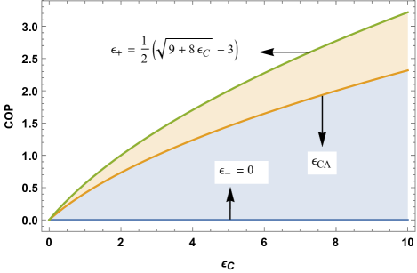
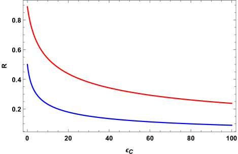
In this section, we compare the CP obtained at maximum $\chi$-function with the optimal CP. As CP can be optimized with respect to $\omega_{c}$ only, we can make the comparison only for this case. Dividing Eq. (LABEL:E55) by Eq. (17), we get the ratio of CP at maximum $\chi$-function to the optimal CP, for the limiting case $\gamma\rightarrow 0$:

$$R_{\gamma\rightarrow 0}=\frac{(3+2\epsilon_{\rm C})\sqrt{9+8\epsilon_{\rm C}}-9-10\epsilon_{\rm C}}{2\epsilon_{\rm C}^{2}},$$ (29)

which approaches the value 8/9 for small $\epsilon_{\rm C}$, while it vanishes for large $\epsilon_{\rm C}$ (small temperature differences).

Similarly, we get the corresponding ratio for $\gamma\rightarrow\infty$ upon dividing Eq. (49) by Eq. (18):

$$R_{\gamma\rightarrow\infty}=\frac{\sqrt{1+\epsilon_{\rm C}}-1}{\epsilon_{\rm C}},$$ (30)

which approaches the value 1/2 for small $\epsilon_{\rm C}$, while it vanishes for large $\epsilon_{\rm C}$. We have plotted Eqs. (29) and (30) in Fig. 5, from which it is clear that the ratio is greater for the case $\gamma\rightarrow 0$. Further, it is interesting to note that although both $R_{\gamma\rightarrow 0}$ and $R_{\gamma\rightarrow\infty}$ vanish for $\epsilon_{\rm C}\rightarrow\infty$, their ratio ${R_{\gamma\rightarrow 0}}/{R_{\gamma\rightarrow\infty}}\to 2\sqrt{2}$ for small temperature differences.

Figure 5: (Color online) Ratio ($R$) of the CP at optimal $\chi$-function to the optimal CP. Red and blue curves represent Eqs. (29) and (30), respectively, which approach the value 8/9 and 1/2 respectively for $\epsilon_{\rm C}\rightarrow 0$, and vanish for $\epsilon_{\rm C}\rightarrow\infty$.

VI Conclusions

In this work, we have studied the optimal performance of a three-level atomic system working as a refrigerator. We have studied two different target functions: CP and $\chi$-function. Although, in many classical and quantum models of the refrigerator, CP is not a good figure of merit to optimize, in our model, it is a well-behaved function and we have obtained analytic expressions for lower and upper bounds on the COP already derived in some models of classical and quantum refrigerators. However, we notice that CP is optimizable only with respect to the control frequency $\omega_{c}$ and thus, we can perform optimization in local region of the parameter space only. In contrast to the behavior of CP, $\chi$-function shows global maximum which makes it a more suitable figure of merit to study the optimal performance of refrigerators. In the general unconstrained regime, we have presented results of numerical optimization in Table I. Then in the low-temperatures regime, we showed that the COP of our model is independent of system-bath coupling ($\Gamma_{c,h}$) or matter-field coupling ($\lambda$), and depends on Carnot COP only, which is a remarkable result. Further, in the high temperature and strong-coupling regime, we have alternatively performed maximization of $\chi$-function with respect to $\omega_{h}$ ($\omega_{c}$ fixed) and $\omega_{c}$ ($\omega_{h}$ fixed). In both cases, we were able to obtain the lower and upper limits on the COP, already well known in the literature on optimization of refrigerators. The possibility of simultaneous optimization of CP and $\chi$-function, enables a comparison between optimal CP in the quantum refrigerator with the CP at optimal $\chi$-function, and we conclude that a large system-bath coupling at the cold end (compared to the hot end) yields a higher relative value of CP (see Fig. 5). There are a few classical models Apertet et al. (2013); Izumida et al. (2013, 2015) in which both CP and $\chi$-function are optimizable. To the best of our knowledge, the present model provides an instance of a quantum thermal machine allowing the same feature. This will aid future studies Mani and Benjamin (2019) which explore models in which the performance of quantum machines can be bettered over their classical counterparts.

Appendix A Steady state solution of density matrix equations

Here, we solve the equations for density matrix in the steady state. Substituting the expressions for $H_{0}$, $\bar{H}$, $V_{0}$, and using Eqs. (4) and (5) in Eq. (6), the time evolution of the elements of the density matrix are given by following equations:

$$\dot{\rho}_{11} = i\lambda(\rho_{10}-\rho_{01})-2\Gamma_{h}[(n_{h}+1)\rho_{11}-n_{h}\rho_{gg}],$$ (31)

$$\dot{\rho}_{00} = -i\lambda(\rho_{10}-\rho_{01})-2\Gamma_{c}[(n_{c}+1)\rho_{00}-n_{c}\rho_{gg}],$$ (32)

$$\dot{\rho}_{10} = -[\Gamma_{h}(n_{h}+1)+\Gamma_{c}(n_{c}+1)]\rho_{10}+i\lambda(\rho_{11}-\rho_{00}),$$

$$\rho_{11} = 1-\rho_{00}-\rho_{gg},$$ (34)

$$\dot{\rho}_{01} = \dot{\rho}_{10}^{*}.$$ (35)

Solving Eqs. (31) - (35) in the steady state by setting $\dot{\rho}_{mn}=0$ ($m,n=0,1$), we obtain

$$\rho_{10}=\frac{i\lambda(n_{h}-n_{c})\Gamma_{c}\Gamma_{h}}{\lambda^{2}[(1+3n_{h})\Gamma_{h}+(1+3n_{c})\Gamma_{c}]+\Gamma_{c}\Gamma_{h}[1+2n_{h}+n_{c}(2+3n_{h})][(1+n_{c})\Gamma_{c}+(1+n_{h})\Gamma_{h}]},$$ (36)

and

$$\rho_{01}=\rho_{10}^{*}.$$ (37)

Calculating the trace in Eq. (7), the input power is given by

$$P=i\hbar\lambda(\omega_{h}-\omega_{c})(\rho_{10}-\rho_{01}).$$ (38)

Similarly evaluating the trace in Eq. (8), heat flux $\dot{Q}_{c}$ can be written as

$$\dot{Q}_{c}=\hbar\omega_{c}(2\Gamma_{c}[n_{c}\rho_{gg}-(n_{c}+1)\rho_{00}]).$$ (39)

Using the steady state condition $\dot{\rho}_{00}=0$ (see Eq. (31)), Eq. (39) becomes

$$\dot{Q}_{c}=i\hbar\lambda\omega_{c}(\rho_{10}-\rho_{01}).$$ (40)

Substituting Eqs. (36) and (37) in Eq. (40), we have

$$\dot{Q_{c}}=\frac{2\hbar\lambda^{2}\Gamma_{c}\Gamma_{h}(n_{c}-n_{h})\omega_{c}}{\lambda^{2}[(1+3n_{h})\Gamma_{h}+(1+3n_{c})\Gamma_{c}]+\Gamma_{c}\Gamma_{h}[1+2n_{h}+n_{c}(2+3n_{h})][(1+n_{c})\Gamma_{c}+(1+n_{h})\Gamma_{h}]}.$$ (41)

The expression for $\chi$-function, $\chi=\epsilon\dot{Q_{c}}$, is given by

$$\chi=\frac{2\hbar\lambda^{2}\Gamma_{c}\Gamma_{h}(n_{c}-n_{h})\omega_{c}^{2}}{\lambda^{2}(\omega_{h}-\omega_{c})[(1+3n_{h})\Gamma_{h}+(1+3n_{c})\Gamma_{c}]+\Gamma_{c}\Gamma_{h}[1+2n_{h}+n_{c}(2+3n_{h})][(1+n_{c})\Gamma_{c}+(1+n_{h})\Gamma_{h}]}.$$ (42)

For refrigerator, $n_{c}>n_{h}$, and thus $\dot{Q}_{c},\chi>0$.

Appendix B Optimization of $\chi$-function with respect to $\omega_{c}$ in high-temperature and strong coupling regime

The expression for the $\chi$-function is given by

$$\chi=\frac{2\hbar\Gamma_{h}\omega_{c}^{2}(\tau\omega_{h}-\omega_{c})}{(\tau\omega_{h}+\gamma\omega_{c})(\omega_{h}-\omega_{c})}.$$ (43)

As explained in the Section IV, we cannot optimize the above function with respect to $\omega_{c}$ to obtain the roots in real radicals because of the Casus irreducibilis (see Appendix C). However, we can obtain the real solutions for the limiting cases $\gamma\rightarrow 0$ and $\gamma\rightarrow\infty$. For $\gamma\rightarrow 0$, $\chi$-function can be written as

$$\chi=\frac{2\hbar\Gamma_{h}\omega_{c}^{2}(\tau\omega_{h}-\omega_{c})}{\tau\omega_{h}(\omega_{h}-\omega_{c})},$$ (44)

which can be optimized to give

$$\omega_{c}=\frac{\omega_{h}}{4}\Big{(}3+\tau-\sqrt{9-10\tau+\tau^{2}}\Big{)}.$$ (45)

Substituting Eq. (45) in Eq. (44) and in the equation $\dot{Q_{c}}=2\hbar\Gamma_{h}\omega_{c}(\tau\omega_{h}-\omega_{c})/\tau\omega_{h}$, we get following expressions for the optimal $\chi$-function and CP at optimal $\chi$-function, respectively:

$$\chi^{*(\omega_{h})}_{\gamma\rightarrow 0} = \hbar\Gamma_{h}\omega_{h}\frac{27+36\epsilon_{\rm C}+8\epsilon_{\rm C}^{2}-(9+8\epsilon_{\rm C})^{3/2}}{4\epsilon_{\rm C}(1+\epsilon_{\rm C})},$$

$$\dot{Q_{c}}^{\chi(\omega_{h})}_{\gamma\rightarrow 0} = \hbar\Gamma_{h}\omega_{h}\frac{(3+2\epsilon_{\rm C})\sqrt{9+8\epsilon_{\rm C}}-9-10\epsilon_{\rm C}}{4\epsilon_{\rm C}(1+\epsilon_{\rm C})}.$$

Similarly, for $\gamma\rightarrow\infty$, optimization of $\chi$-function, $\chi=2\hbar\Gamma_{c}(\tau\omega_{h}-\omega_{c})/(\omega_{h}-\omega_{c})$, yields the following expressions:

$$\chi^{*(\omega_{h})}_{\gamma\rightarrow\infty} = \frac{2\hbar\Gamma_{c}\omega_{h}(2+\epsilon_{\rm C}-\sqrt{1+\epsilon_{\rm C}})}{1+\epsilon_{\rm C}},$$ (48)

$$\dot{Q_{c}}^{\chi(\omega_{h})}_{\gamma\rightarrow\infty} = \frac{2\hbar\Gamma_{c}\omega_{h}(\sqrt{1+\epsilon_{\rm C}}-1)}{1+\epsilon_{\rm C}}.$$ (49)

Appendix C Casus Irreducibilis

In algebra, Casus irreducibilis arises while solving a cubic equation. The formal statement of the Casus irreducibilis is that if a cubic polynomial is irreducible with rational coefficients and has three real roots, then the roots of the cubic equation are not expressible using real radicals and thus, one must introduce expressions with complex radicals, even though the resulting expressions are actually real-valued. It was proven by P. Wantzel in 1843 Kleiner (2007). Using the discriminant $D$ of the irreducible cubic equation, one can decide whether the given equation is in Casus irreducibilies or not, via Cardano’s formula Stewart (1990). The most general form of a cubic equation is given by

$$ax^{3}+bx^{2}+cx+d=0$$ (50)

where $a,b,c,d$ are real.

The discriminant $D$ is given by: $D=18abcd-4b^{3}d+b^{2}c^{2}-4ac^{3}-27a^{2}d^{2}$. Depending upon the sigh of $D$, following three cases arise:
(a) $D<0$, the cubic equation has two complex roots, so Casus irresucibilies does not apply.
(b) $D=0$, all three roots are real and expressible by real radicals.
(c) $D>0$, three are three distinct real roots. In this case, a rational root exists and can be found using the rational root test. Otherwise, the given polynomial is Casus irreducibilis and we need complex valued expressions to express the roots in radicals.

In our case, in order to solve Eq. (27), we have to solve the following cubic equation

$$\gamma\omega_{c}^{3}+2\omega_{h}(\tau-\gamma)\omega_{c}^{2}-\tau\omega_{h}^{2}(3+\tau-\gamma)\omega_{c}+2\tau^{2}\omega_{h}^{3}=0.$$ (51)

The discriminant $D$ of the above equation is given by

$$D=4\omega_{h}^{6}(1+\gamma)(1+\tau)[3\gamma^{2}(3-\tau)+\gamma^{3}+9\gamma\tau+3\gamma\tau^{2}+9\tau^{2}(1-\tau)].$$ (52)

Since the parameters $\omega_{h},\gamma,\tau$ are positive and $\tau<1$, $D>0$. So the polynomial in Eq. (51) presents the case of Casus irreducibilis.

Appendix D Mapping to Feynman’s ratchet and pawl model

It is interesting to note that in the low-temperatures regime, SSD refrigerator can be mapped to Feynman’s ratchet and pawl model Feynman et al. (2008); Parrondo and Espanol (1996); Sheng et al. (2014); Singh and Johal (2017, 2018), a mesoscopic steady-state heat engine capable of extracting work from thermal fluctuations from a setup of two heat reservoirs via a ratchet and pawl mechanism. In the refrigerator mode, the ratchet makes a backward jump when $x_{c}$ amount of heat is absorbed from the cold reservoir and subsequently $x_{h}$ amount of heat is supplied to the hot reservoir Feynman et al. (2008); Singh and Johal (2017). Similarly, the wheel turns in the forward direction when $x_{h}$ energy is absorbed from the hot reservoir. The rates of forward and backward jumps are given by

$$R_{F}=r_{0}e^{-\hbar x_{h}/k_{\rm B}T_{h}},\qquad R_{B}=r_{0}e^{-\hbar x_{c}/k_{\rm B}T_{c}},$$ (53)

where $r_{0}$ is the rate constant. The system operates as a refrigerator when $R_{B}>R_{F}$. The rates of heat exchanged with the cold and hot reservoirs, respectively, are given by

$$\dot{Q}_{c} = x_{c}(R_{B}-R_{F})=r_{0}x_{c}(e^{-\hbar x_{c}/k_{\rm B}T_{c}}-e^{-\hbar x_{h}/k_{\rm B}T_{h}}),$$

$$\dot{Q}_{h} = x_{h}(R_{B}-R_{F})=r_{0}x_{h}(e^{-\hbar x_{c}/k_{\rm B}T_{c}}-e^{-\hbar x_{h}/k_{\rm B}T_{h}}).$$

Therefore, $\chi$-function for Feynman’s model can be written as follows

$$\chi_{\rm F}=\frac{r_{0}x_{c}^{2}}{x_{h}-x_{c}}\left(e^{-\hbar x_{c}/k_{\rm B}T_{c}}-e^{-\hbar x_{h}/k_{\rm B}T_{h}}\right).$$ (56)

Apart from the multiplicative constant $2\hbar\lambda^{2}\Gamma_{c}\Gamma_{h}/(\Gamma_{c}+\Gamma_{h})(\lambda^{2}+\Gamma_{c}\Gamma_{h})$ (instead of $r_{0}$), the expression in Eq. (19) is similar to the $\chi$-function for the Feynman’s model [Eq.(56)], where $\omega_{c}$ and $\omega_{h}$ are replaced by $x_{c}$ and $x_{h}$. Thus, we establish a mapping between our model of refrigerator and Feynman’s model. A similar mapping also exists between the SSD engine and Feynman’s ratchet as heat engine Singh and Johal (2019).

References

- Yan and Chen (1990) Z. Yan and J. Chen, J. Phys. D: Appl. Phys. 23, 136 (1990).
- Agrawal and Menon (1990) D. C. Agrawal and V. J. Menon, J. Phys. A 23, 5319 (1990).
- Allahverdyan et al. (2010) A. E. Allahverdyan, K. Hovhannisyan, and G. Mahler, Phys. Rev. E 81, 051129 (2010).
- Apertet et al. (2013) Y. Apertet, H. Ouerdane, A. Michot, C. Goupil, and P. Lecoeur, Europhys. Lett. 103, 40001 (2013).
- Curzon and Ahlborn (1975) F. L. Curzon and B. Ahlborn, Am. J. Phys. 43, 22 (1975).
- Esposito et al. (2010) M. Esposito, R. Kawai, K. Lindenberg, and C. Van den Broeck, Phys. Rev. Lett. 105, 150603 (2010).
- Izumida, Y. and Okuda, K. (2012) Izumida, Y. and Okuda, K., Europhys. Lett. 97, 10004 (2012).
- Johal (2010) R. S. Johal, Phys. Rev. E 82, 061113 (2010).
- Thomas and Johal (2015) G. Thomas and R. S. Johal, J. Phys. A 48, 335002 (2015).
- Johal (2018) R. S. Johal, Europhys. Lett. 121, 50009 (2018).
- de Tomás et al. (2012) C. de Tomás, A. C. Hernández, and J. M. M. Roco, Phys. Rev. E 85, 010104 (2012).
- Izumida et al. (2013) Y. Izumida, K. Okuda, A. C. Hernández, and J. Roco, Europhys. Lett. 101, 10005 (2013).
- Velasco et al. (1997) S. Velasco, J. M. M. Roco, A. Medina, and A. C. Hernández, Phys. Rev. Lett. 78, 3241 (1997).
- Johal (2019) R. S. Johal, arXiv:1906.02453 (2019).
- Abah and Lutz (2016) O. Abah and E. Lutz, Europhys. Lett. 113, 60002 (2016).
- Correa et al. (2014a) L. A. Correa, J. P. Palao, G. Adesso, and D. Alonso, Phys. Rev. E 90, 062124 (2014a).
- Scovil and Schulz-DuBois (1959) H. E. D. Scovil and E. O. Schulz-DuBois, Phys. Rev. Lett. 2, 262 (1959).
- Geusic et al. (1959) J. E. Geusic, E. O. Schulz-DuBois, R. W. De Grasse, and H. E. D. Scovil, J. Appl. Phys. 30, 1113 (1959).
- Kosloff (2013) R. Kosloff, Entropy 15, 2100 (2013).
- Mahler (2014) G. Mahler, Quantum thermodynamic processes: Energy and information flow at the nanoscale (Jenny Stanford Publishing, 2014).
- Vinjanampathy and Anders (2016) S. Vinjanampathy and J. Anders, Contemp. Phys. 57, 545 (2016).
- Millen and Xuereb (2016) J. Millen and A. Xuereb, New J. Phys. 18, 011002 (2016).
- Deffner and Campbell (2019) S. Deffner and S. Campbell, Quantum Thermodynamics (Morgan & Claypool Publishers, 2019).
- Alicki and Kosloff (2018) R. Alicki and R. Kosloff, in Thermodynamics in the Quantum Regime (Springer, 2018) pp. 1–33.
- Binder et al. (2018) F. Binder, L. A. Correa, C. Gogolin, J. Anders, and G. Adesso, Thermodynamics in the Quantum Regime: Fundamental Aspects and New Directions (Springer, 2018).
- Geva and Kosloff (1994) E. Geva and R. Kosloff, Phys. Rev. E 49, 3903 (1994).
- Geva and Kosloff (1996) E. Geva and R. Kosloff, J. Chem. Phys. 104, 7681 (1996).
- Kosloff and Levy (2014) R. Kosloff and A. Levy, Annu. Rev. Phys. Chem. 65, 365 (2014).
- Dorfman et al. (2018) K. E. Dorfman, D. Xu, and J. Cao, Phys. Rev. E 97, 042120 (2018).
- Singh and Johal (2019) V. Singh and R. S. Johal, Phys. Rev. E 100, 012138 (2019).
- Jaseem et al. (2018) N. Jaseem, M. Hajdušek, V. Vedral, R. Fazio, L. C. Kwek, and S. Vinjanampathy, arXiv:1812.10082 (2018).
- Klatzow et al. (2019) J. Klatzow, J. N. Becker, P. M. Ledingham, C. Weinzetl, K. T. Kaczmarek, D. J. Saunders, J. Nunn, I. A. Walmsley, R. Uzdin, and E. Poem, Phys. Rev. Lett. 122, 110601 (2019).
- Linden et al. (2010) N. Linden, S. Popescu, and P. Skrzypczyk, Phys. Rev. Lett. 105, 130401 (2010).
- Levy and Kosloff (2012) A. Levy and R. Kosloff, Phys. Rev. Lett. 108, 070604 (2012).
- Correa et al. (2013) L. A. Correa, J. P. Palao, G. Adesso, and D. Alonso, Phys. Rev. E 87, 042131 (2013).
- Agarwalla et al. (2017) B. K. Agarwalla, J.-H. Jiang, and D. Segal, Phys. Rev. B 96, 104304 (2017).
- Kilgour and Segal (2018) M. Kilgour and D. Segal, Phys. Rev. E 98, 012117 (2018).
- Holubec and Novotný (2019) V. Holubec and T. Novotný, J. Chem. Phys. 151, 044108 (2019).
- Maslennikov et al. (2019) G. Maslennikov, S. Ding, R. Hablützel, J. Gan, A. Roulet, S. Nimmrichter, J. Dai, V. Scarani, and D. Matsukevich, Nat. Commun. 10, 202 (2019).
- Mitchison et al. (2016) M. T. Mitchison, M. Huber, J. Prior, M. P. Woods, and M. B. Plenio, Quantum Science and Technology 1, 015001 (2016).
- Brask and Brunner (2015) J. B. Brask and N. Brunner, Phys. Rev. E 92, 062101 (2015).
- Gorini et al. (1976) V. Gorini, A. Kossakowski, and E. C. G. Sudarshan, J. Math. Phys. 17, 821 (1976).
- Lindblad (1976) G. Lindblad, Commun. Math. Phys. 48, 119 (1976).
- Boukobza and Tannor (2006a) E. Boukobza and D. J. Tannor, Phys. Rev. A 74, 063823 (2006a).
- Boukobza and Tannor (2006b) E. Boukobza and D. J. Tannor, Phys. Rev. A 74, 063822 (2006b).
- Boukobza and Tannor (2007) E. Boukobza and D. J. Tannor, Phys. Rev. Lett. 98, 240601 (2007).
- Alicki (1979) R. Alicki, J. Phys. A 12, L103 (1979).
- Kosloff (1984) R. Kosloff, J. Chem. Phys. 80, 1625 (1984).
- Geva and Kosloff (1992) E. Geva and R. Kosloff, J. Chem. Phys. 96, 3054 (1992).
- Abah et al. (2012) O. Abah, J. Roßnagel, G. Jacob, S. Deffner, F. Schmidt-Kaler, K. Singer, and E. Lutz, Phys. Rev. Lett. 109, 203006 (2012).
- Correa et al. (2014b) L. A. Correa, J. P. Palao, D. Alonso, and G. Adesso, Sci. Rep 4, 3949 (2014b).
- Uzdin and Kosloff (2014) R. Uzdin and R. Kosloff, Europhys. Lett. 108, 40001 (2014).
- Izumida et al. (2015) Y. Izumida, K. Okuda, J. M. M. Roco, and A. C. Hernández, Phys. Rev. E 91, 052140 (2015).
- Yuan et al. (2014) Y. Yuan, R. Wang, J. He, Y. Ma, and J. Wang, Phys. Rev. E 90, 052151 (2014).
- Wang et al. (2012) Y. Wang, M. Li, Z. C. Tu, A. C. Hernández, and J. M. M. Roco, Phys. Rev. E 86, 011127 (2012).
- Kleiner (2007) I. Kleiner, in A History of Abstract Algebra (Springer, 2007) pp. 113–163.
- Stewart (1990) I. Stewart, Galois theory (Chapman and Hall/CRC, 1990).
- Feynman et al. (2008) R. P. Feynman, R. B. Leighton, and M. Sands, The Feynman Lectures on Physics (Narosa Publishing House, New Delhi, India, 2008).
- Parrondo and Espanol (1996) J. M. R. Parrondo and P. Espanol, Am. J. Phys. 64, 1125 (1996).
- Sheng et al. (2014) S. Sheng, P. Yang, and Z. C. Tu, Commun. Theor. Phys. 62, 589 (2014).
- Singh and Johal (2017) V. Singh and R. S. Johal, Entropy 19, 576 (2017).
- Singh and Johal (2018) V. Singh and R. S. Johal, J. Stat. Mech. 2018, 073205 (2018).
- Mani and Benjamin (2019) A. Mani and C. Benjamin, J. Phys. Chem. C 123, 22858 (2019).