NGEMM: Optimizing GEMM for Deep Learning via Compiler-based Techniques
Abstract
Quantization has emerged to be an effective way to significantly boost the performance of deep neural networks (DNNs) by utilizing low-bit computations. Despite having lower numerical precision, quantized DNNs are able to reduce both memory bandwidth and computation cycles with little losses of accuracy. Integer GEMM (General Matrix Multiplication) is critical to running quantized DNN models efficiently, as GEMM operations often dominate the computations in these models. Various approaches have been developed by leveraging techniques such as vectorization and memory layout to improve the performance of integer GEMM. However, these existing approaches are not fast enough in certain scenarios.
We developed NGEMM, a compiler-based GEMM implementation for accelerating lower-precision training and inference. NGEMM has better use of the vector units by avoiding unnecessary vector computation that is introduced during tree reduction. We compared NGEMM’s performance with the state-of-art BLAS libraries such as MKL. Our experimental results showed that NGEMM outperformed MKL non-pack and pack version by an average of 1.86x and 1.16x, respectively. We have applied NGEMM to a number of production services in Microsoft.
Keywords Deep Learning Training Inference Low-Precision GEMM Compiler
1 Introduction
In the past few years, deep neural networks (DNNs) have demonstrated great success in various domains such as natural language processing (Howard & Ruder,, 2018; Radford et al. ,, 2018), speech recognition (Deng et al. ,, 2013; Anwar et al. ,, 2015) and computer vision (Simonyan & Zisserman,, 2014; Szegedy et al. ,, 2015). The increasing size and complexity of DNN models have become an impediment to the deployment of these models on edge devices where latency is often a hard requirement. Even for cloud platforms like Azure, AWS and Google Cloud, where more computational resources are available, complex models such as BERT (Devlin et al. ,, 2018) may still cause long service time and high cost for both training and inference.
Quantization has emerged to be an effective way to significantly improve the performance of DNN models by utilizing low-bit computations (Krishnamoorthi,, 2018; Jacob et al. ,, 2018; Rastegari et al. ,, 2016a; Han et al. ,, 2015; Lin et al. ,, 2016). By converting the weights and activations of a DNN model from high-precision floating point values to low-precision representations, quantization is able to reduce the model size and hence requires less memory for running the model. Smaller memory footprint can have better cache behavior, because more intermediate computation results can be kept in the cache for re-use. Moreover, computations on lower numerical representations such as 8-bit integers almost always need fewer clock cycles on contemporary general purpose CPUs and GPUs, compared with their high precision counterparts such as 32-bit floating point.
GEMM operations often dominate the computation for training or inferencing DNN models (Jia,, 2014). Consequently, high performant integer GEMM has great impact to the efficiency of quantized DNN models, where high-precision floating point matrix elements are converted to low-bit such as 8-bit integers. Recently, there have been increasing efforts in developing high-performance low-precision GEMM libraries, such as FBGEMM (Daya Khudia & Deng.,, 2018), gemmlowp (Jacob et al. ,, 2017) and MKL (Intel,, 2019), where techniques such as vectorization, memory layout and various tiling schemes (Goto & Geijn,, 2008; Van Zee & Van De Geijn,, 2015) are applied to optimize GEMM computation. However, they are still not fast enough in certain scenarios.
We developed NGEMM, an optimized GEMM implementation for DNN models based on compiler techniques. NGEMM can provide high performance GEMM computation with different low-precision representations for various target machines. Our experimental results showed that NGEMM outperformed MKL non-pack and pack version by an average of 1.86x and 1.16x respectively. NGEMM has been used in a number of Microsoft production services (Chang et al. ,, 2018; Microsoft,, 2018)111NGEMM is used as external custom functions for specific integer BLAS routines in our Halide-based inference engine (Chang et al. ,, 2018), and is implemented as a rewriting pass in code generation of Nuphar Execution Provider in ONNX Runtime (Microsoft,, 2018)..
In the rest of the paper, we will be focusing on Intel X86 CPUs, which are ubiquitous in modern computing systems. However, our methodology is widely applicable and not just specific to Intel CPUs.
2 Background
In this section, we briefly discuss the conventional approach to implementing low-precision GEMM.
2.1 Conventional Approach
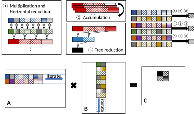
Figure 1 shows the conventional approach (Rodriguez et al. ,, 2018) to conduct low-precision GEMM. Matrix A is the weight matrix with size of , and is typically determined from the training. Matrix B is input matrix, which contains the input data. Matrix C is the result. In low-precision GEMM, matrices A and B are the ones with low numerical precision such as 8- or 16-bit, while matrix C is in higher precision like 32-bit. Throughout the example below, we will use unsigned 8-bit integers for matrix A and signed 8-bit integers for matrix B. Other integer types have similar processes.
In Figure 1, ➀, ➁ and ➂ are the typical phases to perform GEMM vector reduction, which computes the dot product of one row from matrix A and one column from matrix B to produce one element of matrix C. Phase ➀ shows the process of converting low-precision values to higher precision. VPMADDUBSW takes two 8-bit integer vectors, and , which contain unsigned and signed integers loaded from matrix A and B, respectively. It then multiplies each unsigned 8-bit integer in and the corresponding signed 8-bit integer in , produces a signed 16-bit integer. Lastly, it adds adjacent pairs of the 16-bit integers to generate another vector :
After that, VPMADDWD takes and a unit vector to perform horizontal reduction, which produces a signed 32-bit integer vector :
where each 32-bit value in comes from four 8-bit values, thus . The result of phase ➀ is a 32-bit integer vector with size of .
Note that the vector width (i.e. the number of cubes in the vector) in Figure 1 is just for illustration purpose. The actual width depends on the data type and target machine. For example, on an AVX-2 machine, where the vector width is 256 bits, the vector size of is . In contrast, for an AVX512 machine, becomes .
Phase ➁ repeats the computation in Phase ➀ multiple times for the rest of the bytes of the same row from matrix A and the same column from matrix B. Each repetition produces a 32-bit vector , which will be accumulated using instruction VPADDD. This phase gives us: .
Phase ➂ sums all of the 32-bit integers within the vector using tree-reduction to generate one final element in matrix C (shown as the black cube). There are different ways to achieve this phase depends on instructions used. One approach is to use VPHADDD, which is the instruction to horizontally add adjacent pairs of 32-bit integers. Depending on vector width, multiple VPHADDD are needed to accumulate the integer values and generate the final value. The other approach is to utilize the VPSHFD instruction, which shuffles the 32-bit integers within the vector, with following VPADDD to accumulate corresponding values to generate the final result.
Finally, phase ➀ ➁ ➂ are applied to all rows of matrix A and columns of matrix B to generate the whole matrix C. Although these phases change the common reduction order of GEMM, they are typically applicable in integer computation unless overflow happens due to a very large , which is rare for most DNN models, where ranges from 100s to 1000s.
3 Methodology
3.1 Alternative Approach
The conventional approach described in the previous section is straightforward to perform low-precision GEMM computation. However, it is not optimal because the vector units are not fully used during the tree-reduction phase ➂. Therefore, we present NGEMM, which has better use of the vector units by avoiding non-efficient vector computation such as tree-reduction.
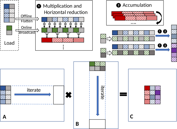
Figure 2 shows the details of our NGEMM. We use the same configuration as that we used for the conventional approach: matrix A is the weight matrix, matrix B is the input matrix, and matrix C is the result matrix. Matrices A and B are in low numerical precision, and matrix C has 32-bit full precision.
Similar to phase ➀ in the conventional approach, phase ❶ computes partial results from two vectors, and , using VPMADDUBSW and VPMADDWD. However, the shapes of the loaded data are different from the conventional approach even with the same vector length. In this illustration, its shape is , which is determined by the vector width and the width of horizontal reduction in practise. For example, the shape is for AVX2. Because both dimensions are shorter than the vector width, loads of access non-contiguous memory, which may compromise memory bandwidth. To resolve the issue, we apply data layout transformation (see Sec 3.1.1) to force to be fully contiguous in memory.
Furthermore, because vector has shorter length than (), we broadcast to :
where has the same width as . For example, if , then , Consequently, and will be as follows:
Figure 2 shows an example of (two elements during load of matrix B) for simplicity, which is the 16-bit scenario:
where only VPMADDWD is required in phase ❶ to accumulate to 32-bit.
The second phase ❷ accumulates all the partial results of to directly form the final result vector in matrix C.
Figure 2 also shows the two more partial results obtained by applying phases ❶ and ❷ to the same part of A but different two vectors of B. The same computation will be applied to the entire A and B and obtain the final result matrix C.
Compared with phases ➀ ➁ ➂ of the conventional approach, our approach only has phases ❶ and ❷ but missing the tree-reduction phase, which is implicitly finished through the vector additions in phase ❷.
Our presented approach is not limited to GEMM operations, but benefits other similar computations such as GEMV. Moreover, it is also applicable to GEMM operations with other types such as signed 16-bit or unsigned 8-bit integers.
It is worthwhile to mention that Intel adopted similar approach in MKL (Andres Rodriguez,, 2018), which is contemporary work with our NGEMM.
3.1.1 Data Layout
We describe the data layout used by our approach in detail. The layout is mainly for the weight matrix in a DNN model, e.g. matrix A in our examples. Therefore, data marshalling can often be performed offline. For those uncommon cases where both matrices are inputs, we can simply perform online packing with extra overhead.

Figure 3 and Figure 4 demonstrates the two-level hierarchy of the layout used in NGEMM. Figure 3 shows various inner layouts in NGEMM, where the top row display the original vector access. Assuming the memory address grows horizontally, the original vector loads the contiguous elements from the memory. Vector width depends on hardware instructions and data types as displayed in Figure 3:
The bottom row draws the inner layout, which determines the data access pattern for the matrix. Instead of accessing data from a single row or column, inner layout will first access elements along dimension and then move to next row, and repeat this process times along M dimension. This kind of memory access forms a small zigzag pattern, which is known as Morton code (Morton,, 1966). Usually, and are determined by hardware instructions and data type:
The size of simply implies the number of elements needed to be accumulated to a single 32-bit value in phase (❶).
Figure 4 illustrates the outer layout pattern in NGEMM for weight matrix. The outer layout can be combined with loop optimizations such as loop tiling to deliver better performance. Loop tiling is a classic loop transformation technique to maximize parallelism and improve cache locality (Hong et al. ,, 2016; Bao et al. ,, 2017b, a). It has been widely adopted in various BLAS libraries to optimize intensive computation such as GEMM.
Figure 4 (a) shows the outer layout without loop tiling applied, which iterate the inner layout pattern first through M dimension and then K dimension for the whole matrix. It is worth mentioning that if columns or rows are not multiple of or , we simply pad 0-element, respectively.
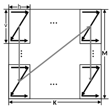
(a) Outer layout without tiling
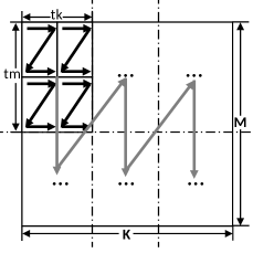
(b) Outer layout with tiling
Figure 4 (b) shows the tiling with a tile size -by- combined with the layout for matrix A, where denote tiling sizes along dimension of the GEMM. In our tiling scheme, -by- typically contains multiple -by-. Thus the tiling size selection of becomes , where is the tiling size along dimension N. The outer layout then is to iterate the tile pattern through the whole matrix.
Moreover, we also apply inter- and intra- tile level optimizations. For inter-tile level, we perform loop unrolling to increase locality and reduce loop control overhead within a tile. For intra-tile level, different loop permutation can be used, which corresponds to the outer layout iterate order described previously. Overall, the loop tiling size and permutation are a typical search-space-exploration problem, which can be solved by techniques such as auto-tuning.
3.2 Latency Analysis
In this part, we perform the latency analysis between the conventional approach and our NGEMM. Note, here, we only considers the computation cost, but ignores the cost of loads/stores, since after data layout transformation, memory accesses in the both methods have become contiguous.
Assume the matrix sizes are the same as previous section, i.e. with vector width . The latency of the conventional approach can be calculated as follows:
where and are the total cost for phase ➀ and ➁ in the conventional approach respectively. Here, is the latency cost of tree-reduction computation , and is constant parameter.
For our NGEMM with layout size , the latency is as follows:
where latency(❶) and latency(❷) are the time cost of phase ❶ and ❷ in NGEMM. The speedup ratio between these two can be expressed as:
| (1) |
where phases of ➀ ➁ and ❶ ❷ have the same latency cost, and their latency can be noted as . Then equation (1) can be expressed as:
| (2) |
where represents the reduction dimension in the step of vector width of matrix multiplication, is the vector width and is constant parameter.
From equation (2), we can observe that the speedup is relevant to reduction dimension and vector width. The longer vector width and the shorter reduction dimension will result in better speedup. It is worth mentioning that the trend of increasing vector width continues in new generation of processors.
4 Implementation
We implemented single-threaded NGEMM by leveraging TVM (Chen et al. ,, 2018) tensorize schedule primitive that replaces partial computation code with the corresponding intrinsics in LLVM (Lattner & Adve,, 2004). It can be easily extended to support multi-threading by parallelizing the outermost loop. We modified TVM code to properly handle tail condition during code generation, which is important for certain loop transformation techniques (Bao et al. ,, 2016a; Bao,, 2018). Furthermore, we added several LLVM intrinsics that were not supported by TVM. It is worthwhile to mention that our NGEMM is not limited to TVM. The same techniques can be implemented in other compiler-based frameworks (Rotem et al. ,, 2018; Google,, 2019).
Layout The layout of the weight matrix has been prepacked offline, and the marshalled matrix is fed as a constant initializer to the inference runtime. NGEMM generates different layouts for the weight matrix based on numerical precision requirements and supported instruction sets.
Loop Optimization The optimal loop tiling sizes and permutation orders are determined through compiler auto-tuning. NGEMM generates the best choice based on matrix sizes, target machines and numerical precision.
Moreover, it is straightforward to explore more extensions such as operation fusion with the help of compiler techniques. DNN models have pre- and post-GEMM operations, which can be fused together with GEMM to increase cache locality and thus improve performance.
5 Evaluation
We evaluated NGEMM’s performance against MKLML in MKL-DNN v0.21222This version of MKL fixed certain performance issues in previous versions.. Our NGEMM was implemented in ONNX Runtime (Microsoft,, 2018), using a custom version of TVM with LLVM 9.0.0. The experiments were conducted on a machine with 8-core 2.3GHz Intel Xeon E5-2673V4 processors where AVX2 is supported. The machine runs Ubuntu 16.04 and GCC 6.5. No frequency scaling (DVFS) related techniques were used in the experiments (Bao et al. ,, 2016b; Farkas et al. ,, 2000). The performance numbers were obtained by taking ggeometric means across repetitions after several warmup runs. The numbers include only function calls of MKL rountines or our generated functions, without any ML framework overhead333Speedup numbers reported in the previous version include ONNX Runtime overhead..
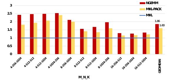
Figure 5 shows the speedups of NGEMM and MKL-PACK (the pack version with the routines cblas_gemm_s8u8s32_compute and the offline packing routines cblas_gemm_s8u8s32_pack) over non-pack MKL (the version with the routines cblas_gemm_s8u8s32) on various problem sizes with 8-bit integers. Similar to NGEMM, MKL-PACK applies packing to the weight matrix. In contrast, MKL does not do any packing. The last two bars in the figure are the geometric means of the speedups of NGEMM and MKL-PACK over MKL across all the problem sizes. NGEMM and MKL-PACK demonstrated 1.86x and 1.60x speedups compared to MKL, respectively.
As shown in the graph, NGEMM has better performance compared to MKL for all the problem sizes that we chosen. NGEMM also shows about 1.16X speedups over MKL-PACK. Moreover, we observed a huge memory cost (about 12MB) with MKL-PACK for packing a [] int8 weight matrix, whereas NGEMM consumed only 0.25MB, which is the size of the matrix.
It is worth mentioning that the actual performance benefits of NGEMM might vary for different deep learning models. Real models have computations performed by other ops such as element-wise ops, which consume considerable time. In our experiments with real production models, NGEMM could delivered up to 1.34X speedups over MKL without packing.
6 Related work
Many research studies (Vanhoucke et al. ,, 2011; Rastegari et al. ,, 2016b; Mellempudi et al. ,, 2017; Das et al. ,, 2018) have shown that low numerical precision can be applied to DNN models with minimal to no accuracy losses. Quantization techniques have been adopted by many DNN frameworks to improve training and inference performance. XLA (Accelerated linear algebra) (Leary & Wang,, 2017) is a compiler backend for TensorFlow (Abadi et al. ,, 2016), which supports various optimizations including quantization and generate machine instructions for different targets. Glow (Rotem et al. ,, 2018) is a machine learning compiler, which consumes neural network graphs, performs high-level graph optimizations and low-level machine-dependent optimizations for diverse hardware targets. Glow also supports quantization with various bit-widths. TVM (Chen et al. ,, 2018), another compiler stack for deep learning, compiles the model into low-level IR and performs loop optimizations. It supports multiple hardware backends and quantization with different bit-widths. Our work, NGEMM, incorporates with Microsoft ONNX Runtime (Microsoft,, 2018).
Many BLAS libraries, meanwhile, have implemented low precision GEMM for various architectures. Intel MKL (Math Kernel Library) (Wang et al. ,, 2014) provides well tuned 8- and 16-bit GEMM kernels, which is widely adopted across many DNN frameworks as a CPU vendor library. NVIDIA cuBLAS library (Nvidia,, 2008) provides GPU counterparts on NVIDIA GPUs. FBGEMM (Daya Khudia & Deng.,, 2018) is a reduced-precision linear algebra library for deep learning inference, and is integrated into Caffe2. Gemmlowp (Jacob et al. ,, 2017) is a library that only supports low-precision GEMM. In addition to execution time, it is also optimized to minimize the power consumption, which is crucial for edge devices.
Other than TVM, which is used to implement our techniques in the paper, general-purpose code generation frameworks (Chen et al. ,, 2008; Püschel et al. ,, 2004; Chang et al. ,, 2016; Chang,, 2017; De Gonzalo et al. ,, 2019), and domain-specific languages (Ragan-Kelley et al. ,, 2013; Sujeeth et al. ,, 2014), are also capable to adopt our techniques for optimizing GEMM routines.
7 Conclusion
In this paper, we present NGEMM, an optimized low-precision GEMM implementation based on compiler techniques. Compared to the conventional approach adopted by contemporary BLAS libraries, our approach does not require tree reduction and hence has better performance. We implemented a hierarchical layout for the weight matrix to further improve the latency. Our evaluation on various problem sizes demonstrate an average of 1.16X and 1.86X speedup over state-of-the-art MKL library with and without packing. A number of production models also show up to 1.34X speedup using NGEMM compared to MKL without packing.
References
- Abadi et al. , (2016) Abadi, Martín, Barham, Paul, Chen, Jianmin, Chen, Zhifeng, Davis, Andy, Dean, Jeffrey, Devin, Matthieu, Ghemawat, Sanjay, Irving, Geoffrey, Isard, Michael, et al. . 2016. Tensorflow: A system for large-scale machine learning. Pages 265–283 of: 12th USENIX Symposium on Operating Systems Design and Implementation (OSDI 16).
- Andres Rodriguez, (2018) Andres Rodriguez, Eden S., Etay Meiri Evarist Fomenko Young Jin K. Haihao Shen BARUKH Z. 2018. Lower Numerical Precision Deep Learning Inference and Training.
- Anwar et al. , (2015) Anwar, Sajid, Hwang, Kyuyeon, & Sung, Wonyong. 2015. Fixed point optimization of deep convolutional neural networks for object recognition. Pages 1131–1135 of: 2015 IEEE International Conference on Acoustics, Speech and Signal Processing (ICASSP). IEEE.
- Bao et al. , (2017a) Bao, W, Rawat, P, Kong, M, Krishnamoorthy, S, Pouchet, L, & Sadayappan, P. 2017a. Efficient Cache Simulation for Aine Computations. In: International Workshop on Languages and Compilers for Parallel Computing (LCPC’17).
- Bao, (2018) Bao, Wenlei. 2018. Compiler Techniques for Transformation Verification, Energy Efficiency and Cache Modeling. Ph.D. thesis, The Ohio State University.
- Bao et al. , (2016a) Bao, Wenlei, Krishnamoorthy, Sriram, Pouchet, Louis-Noël, Rastello, Fabrice, & Sadayappan, Ponnuswamy. 2016a. Polycheck: Dynamic verification of iteration space transformations on affine programs. Pages 539–554 of: ACM SIGPLAN Notices, vol. 51. ACM.
- Bao et al. , (2016b) Bao, Wenlei, Hong, Changwan, Chunduri, Sudheer, Krishnamoorthy, Sriram, Pouchet, Louis-Noël, Rastello, Fabrice, & Sadayappan, P. 2016b. Static and dynamic frequency scaling on multicore CPUs. ACM Transactions on Architecture and Code Optimization (TACO), 13(4), 51.
- Bao et al. , (2017b) Bao, Wenlei, Krishnamoorthy, Sriram, Pouchet, Louis-Noel, & Sadayappan, P. 2017b. Analytical modeling of cache behavior for affine programs. Proceedings of the ACM on Programming Languages, 2(POPL), 32.
- Chang, (2017) Chang, Li-Wen. 2017. Toward Performance Portability for CPUs and GPUs Through Algorithmic Compositions. Ph.D. thesis, University of Illinois.
- Chang et al. , (2016) Chang, Li-Wen, Hajj, Izzat El, Rodrigues, Christopher, Gómez-Luna, Juan, & Hwu, Wen-mei. 2016. Efficient Kernel Synthesis for Performance Portable Programming. Pages 12:1–12:13 of: The 49th Annual IEEE/ACM International Symposium on Microarchitecture.
- Chang et al. , (2018) Chang, Li-Wen, Chen, Yang, Bao, Wenlei, Agarwal, Amit, Akchurin, Eldar, Deng, Ke, & Barsoum, Emad. 2018. Accelerating Recurrent Neural Networks through Compiler Techniques and Quantization.
- Chen et al. , (2008) Chen, Chun, Chame, Jacqueline, & Hall, Mary. 2008. CHiLL: A framework for composing high-level loop transformations. Tech. rept.
- Chen et al. , (2018) Chen, Tianqi, Moreau, Thierry, Jiang, Ziheng, Zheng, Lianmin, Yan, Eddie, Shen, Haichen, Cowan, Meghan, Wang, Leyuan, Hu, Yuwei, Ceze, Luis, et al. . 2018. TVM: An automated end-to-end optimizing compiler for deep learning. Pages 578–594 of: 13th USENIX Symposium on Operating Systems Design and Implementation (OSDI 18).
- Das et al. , (2018) Das, Dipankar, Mellempudi, Naveen, Mudigere, Dheevatsa, Kalamkar, Dhiraj, Avancha, Sasikanth, Banerjee, Kunal, Sridharan, Srinivas, Vaidyanathan, Karthik, Kaul, Bharat, Georganas, Evangelos, Heinecke, Alexander, Dubey, Pradeep, Corbal, Jesus, Shustrov, Nikita, Dubtsov, Roma, Fomenko, Evarist, & Pirogov, Vadim. 2018. Mixed Precision Training of Convolutional Neural Networks using Integer Operations.
- Daya Khudia & Deng., (2018) Daya Khudia, Protonu Basu, & Deng., Summer. 2018. Open-sourcing FBGEMM for state-of-the-art server-side inference. https://code.fb.com/ml-applications/fbgemm/.
- De Gonzalo et al. , (2019) De Gonzalo, Simon Garcia, Huang, Sitao, Gómez-Luna, Juan, Hammond, Simon, Mutlu, Onur, & Hwu, Wen-mei. 2019. Automatic Generation of Warp-level Primitives and Atomic Instructions for Fast and Portable Parallel Reduction on GPUs. Pages 73–84 of: Proceedings of the 2019 IEEE/ACM International Symposium on Code Generation and Optimization.
- Deng et al. , (2013) Deng, Li, Hinton, Geoffrey, & Kingsbury, Brian. 2013. New types of deep neural network learning for speech recognition and related applications: An overview. Pages 8599–8603 of: 2013 IEEE International Conference on Acoustics, Speech and Signal Processing. IEEE.
- Devlin et al. , (2018) Devlin, Jacob, Chang, Ming-Wei, Lee, Kenton, & Toutanova, Kristina. 2018. Bert: Pre-training of deep bidirectional transformers for language understanding. arXiv preprint arXiv:1810.04805.
- Farkas et al. , (2000) Farkas, Keith I, Flinn, Jason, Back, Godmar, Grunwald, Dirk, & Anderson, Jennifer M. 2000. Quantifying the energy consumption of a pocket computer and a Java virtual machine. ACM SIGMETRICS Performance Evaluation Review, 28(1), 252–263.
- Google, (2019) Google. 2019. "Multi-Level Intermediate Representation" Compiler Infrastructure. https://github.com/tensorflow/mlir.
- Goto & Geijn, (2008) Goto, Kazushige, & Geijn, Robert A. 2008. Anatomy of high-performance matrix multiplication. ACM Transactions on Mathematical Software (TOMS), 34(3), 12.
- Han et al. , (2015) Han, Song, Pool, Jeff, Tran, John, & Dally, William. 2015. Learning both weights and connections for efficient neural network. Pages 1135–1143 of: Advances in neural information processing systems.
- Hong et al. , (2016) Hong, Changwan, Bao, Wenlei, Cohen, Albert, Krishnamoorthy, Sriram, Pouchet, Louis-Noël, Rastello, Fabrice, Ramanujam, J, & Sadayappan, Ponnuswamy. 2016. Effective padding of multidimensional arrays to avoid cache conflict misses. Pages 129–144 of: ACM SIGPLAN Notices, vol. 51. ACM.
- Howard & Ruder, (2018) Howard, Jeremy, & Ruder, Sebastian. 2018. Universal language model fine-tuning for text classification. arXiv preprint arXiv:1801.06146.
- Intel, (2019) Intel. 2019. Intel Math Kernel Library. https://software.intel.com/en-us/mkl/.
- Jacob et al. , (2017) Jacob, Benoit, et al. . 2017. gemmlowp: a small self-contained low-precision GEMM library.(2017).
- Jacob et al. , (2018) Jacob, Benoit, Kligys, Skirmantas, Chen, Bo, Zhu, Menglong, Tang, Matthew, Howard, Andrew, Adam, Hartwig, & Kalenichenko, Dmitry. 2018. Quantization and training of neural networks for efficient integer-arithmetic-only inference. Pages 2704–2713 of: Proceedings of the IEEE Conference on Computer Vision and Pattern Recognition.
- Jia, (2014) Jia, Yangqing. 2014. Learning semantic image representations at a large scale. Ph.D. thesis, UC Berkeley.
- Krishnamoorthi, (2018) Krishnamoorthi, Raghuraman. 2018. Quantizing deep convolutional networks for efficient inference: A whitepaper. CoRR, abs/1806.08342.
- Lattner & Adve, (2004) Lattner, Chris, & Adve, Vikram. 2004. LLVM: A compilation framework for lifelong program analysis & transformation. Page 75 of: Proceedings of the international symposium on Code generation and optimization: feedback-directed and runtime optimization. IEEE Computer Society.
- Leary & Wang, (2017) Leary, Chris, & Wang, Todd. 2017. XLA: TensorFlow, compiled. TensorFlow Dev Summit.
- Lin et al. , (2016) Lin, Darryl, Talathi, Sachin, & Annapureddy, Sreekanth. 2016. Fixed point quantization of deep convolutional networks. Pages 2849–2858 of: International Conference on Machine Learning.
- Mellempudi et al. , (2017) Mellempudi, Naveen, Kundu, Abhisek, Das, Dipankar, Mudigere, Dheevatsa, & Kaul, Bharat. 2017. Mixed Low-precision Deep Learning Inference using Dynamic Fixed Point.
- Microsoft, (2018) Microsoft. 2018. ONNX Runtime: Cross-platform, high performance scoring engine for ml models. https://github.com/microsoft/onnxruntime.
- Morton, (1966) Morton, Guy M. 1966. A computer oriented geodetic data base and a new technique in file sequencing.
- Nvidia, (2008) Nvidia, CUDA. 2008. Cublas library. NVIDIA Corporation, Santa Clara, California, 15(27), 31.
- Püschel et al. , (2004) Püschel, Markus, Moura, José MF, Singer, Bryan, Xiong, Jianxin, Johnson, Jeremy, Padua, David, Veloso, Manuela, & Johnson, Robert W. 2004. Spiral: A generator for platform-adapted libraries of signal processing alogorithms. International Journal of High Performance Computing Applications, 18(1), 21–45.
- Radford et al. , (2018) Radford, Alec, Narasimhan, Karthik, Salimans, Tim, & Sutskever, Ilya. 2018. Improving language understanding with unsupervised learning. Tech. rept. Technical report, OpenAI.
- Ragan-Kelley et al. , (2013) Ragan-Kelley, Jonathan, Barnes, Connelly, Adams, Andrew, Paris, Sylvain, Durand, Frédo, & Amarasinghe, Saman. 2013. Halide: a language and compiler for optimizing parallelism, locality, and recomputation in image processing pipelines. ACM SIGPLAN Notices, 48(6), 519–530.
- Rastegari et al. , (2016a) Rastegari, Mohammad, Ordonez, Vicente, Redmon, Joseph, & Farhadi, Ali. 2016a. Xnor-net: Imagenet classification using binary convolutional neural networks. Pages 525–542 of: European Conference on Computer Vision. Springer.
- Rastegari et al. , (2016b) Rastegari, Mohammad, Ordonez, Vicente, Redmon, Joseph, & Farhadi, Ali. 2016b. XNOR-Net: ImageNet Classification Using Binary Convolutional Neural Networks. Lecture Notes in Computer Science, 525–542.
- Rodriguez et al. , (2018) Rodriguez, Andres, Segal, Eden, Meiri, Etay, Fomenko, Evarist, Kim, Y Jim, Shen, Haihao, & Ziv, Barukh. 2018. Lower numerical precision deep learning inference and training. Intel White Paper.
- Rotem et al. , (2018) Rotem, Nadav, Fix, Jordan, Abdulrasool, Saleem, Catron, Garret, Deng, Summer, Dzhabarov, Roman, Gibson, Nick, Hegeman, James, Lele, Meghan, Levenstein, Roman, et al. . 2018. Glow: Graph lowering compiler techniques for neural networks. arXiv preprint arXiv:1805.00907.
- Simonyan & Zisserman, (2014) Simonyan, Karen, & Zisserman, Andrew. 2014. Very deep convolutional networks for large-scale image recognition. arXiv preprint arXiv:1409.1556.
- Sujeeth et al. , (2014) Sujeeth, Arvind K., Brown, Kevin J., Lee, Hyoukjoong, Rompf, Tiark, Chafi, Hassan, Odersky, Martin, & Olukotun, Kunle. 2014. Delite: A Compiler Architecture for Performance-Oriented Embedded Domain-Specific Languages. ACM Transactions on Embedded Computing Systems, 13(4s), 134:1–134:25.
- Szegedy et al. , (2015) Szegedy, Christian, Liu, Wei, Jia, Yangqing, Sermanet, Pierre, Reed, Scott, Anguelov, Dragomir, Erhan, Dumitru, Vanhoucke, Vincent, & Rabinovich, Andrew. 2015. Going deeper with convolutions. Pages 1–9 of: Proceedings of the IEEE conference on computer vision and pattern recognition.
- Van Zee & Van De Geijn, (2015) Van Zee, Field G, & Van De Geijn, Robert A. 2015. BLIS: A framework for rapidly instantiating BLAS functionality. ACM Transactions on Mathematical Software (TOMS), 41(3), 14.
- Vanhoucke et al. , (2011) Vanhoucke, Vincent, Senior, Andrew, & Mao, Mark Z. 2011. Improving the speed of neural networks on CPUs.
- Wang et al. , (2014) Wang, Endong, Zhang, Qing, Shen, Bo, Zhang, Guangyong, Lu, Xiaowei, Wu, Qing, & Wang, Yajuan. 2014. Intel math kernel library. Pages 167–188 of: High-Performance Computing on the Intel® Xeon Phi™. Springer.