Analytic integral solutions for induced gravitational waves

Jinn-Ouk Gong Korea Astronomy and Space Science Institute, Daejeon 34055, Korea Department of Science Education, Ewha Womans University, Seoul 03760, Korea Asia Pacific Center for Theoretical Physics, Pohang 37673, Korea
Abstract

We present analytic integral solutions for the second-order induced gravitational waves (GWs). After presenting all the possible second-order source terms, we calculate explicitly the solutions for the GWs induced by the linear scalar and tensor perturbations during matter- and radiation-dominated epochs.

cosmology: theory — large-scale structure of universe — gravitational waves

1 Introduction

A series of detection of the gravitational waves (GWs) by the LIGO and Virgo collaborations (Abbott et al., 2016a, b, 2017a, 2017b, 2017c, 2017d) has opened the era of multi-messenger astronomy led by GWs. The observed GW signals are originated from merging black holes and/or neutron stars, but there should be other events energetic enough to generate observable GWs. Such cosmological origins include cosmic strings (Vachaspati, & Vilenkin, 1985; Brandenberger et al., 1986), phase transition (Witten, 1984; Hogan, 1986) and preheating (Khlebnikov, & Tkachev, 1997). But the non-linear nature of gravity tells us that there is a persistent source of GWs – they can be induced by other cosmological perturbations at non-linear order (Mollerach et al., 2004; Ananda et al., 2007; Baumann et al., 2007): while the scalar-, vector- and tensor-type perturbations are decoupled at linear order, they couple to each other and thus can be generated at non-linear order (Noh, & Hwang, 2004; Hwang, & Noh, 2007). Especially, the second-order tensor perturbations, or GWs, induced by linear scalar perturbations111 It should be noted that large scalar perturbations may well be induced by large tensor perturbations on small scales, leading to copious production of primordial black holes (Nakama & Suyama, 2015, 2016). Such induced scalar perturbations subsequently can further induce tensor perturbations. This is an interesting possibility, but is beyond the scope of the present work. may well be sizable if on small scales the primordial curvature perturbation is enhanced during inflation (Alabidi et al., 2012) or the density perturbation grows during an early matter-dominated (MD) epoch (Assadullahi, & Wands, 2009; Jedamzik et al., 2010; Alabidi et al., 2013).

In most of the literature, however, the study of second-order induced GWs has been focused on MD in one particular gauge choice for the scalar perturbations. The reason could be twofold. First, the (geometric) scalar perturbation remains constant even on sub-horizon scales during MD, but it decays quickly if it enters the horizon during radiation-dominated (RD) epoch [see (29) and (30)]. Thus, even if the primordial curvature perturbation is enhanced on small scales, one would naively expect such an enhancement to disappear during an RD epoch so that there should be no sizable induced GWs from scalar perturbations [see, however, Inomata et al. (2019a, b)]. Furthermore, there is an upper bound on the contribution of the primordial GWs from the observations on the cosmic microwave background (CMB): in terms of the so-called tensor-to-scalar ratio, r<0.07𝑟0.07r<0.07 at the pivot scale k=0.05𝑘0.05k=0.05 Mpc-1 (BICEP2 Collaboration et al., 2016). This means on the CMB scales the amplitude of the primordial GWs should be about 1/10 or even smaller than that of the primordial curvature perturbation. Thus, naturally scalar perturbations should be the most dominant source for the induced GWs compared to the other types of cosmological perturbations. For these reasons, it is very sensible to consider the induced GWs by scalar perturbations during MD.

Nevertheless, this does not mean at all that we have a complete and satisfactory understanding of the second-order induced GWs. First, there is no a priori reason why scalar perturbations should be considered only in a particular gauge condition. Moreover, as the linear scalar perturbations depend on the choice of gauge, the second-order GWs induced by their quadratic combinations should be also dependent on the gauge conditions. This is obvious and indeed was noticed early (Arroja et al., 2009) but was explicitly shown only recently in Hwang et al. (2017). Second, while scalar perturbations are likely to be the most important source for the induced GWs, other types of perturbations need not be neglected from the beginning. Especially, the linear tensor perturbations should be persistent. Furthermore, it is possible that the contributions of the tensor perturbations can be enhanced (Mukhanov, & Vikman, 2006), thus, the induced second-order GWs from them may well be significant accordingly222 More exactly, if the tensor-induced GWs are to be dominant, the scalar perturbations should not increase. Otherwise, the scalar-induced GWs are very likely to be more prominent than the tensor-induced ones. This condition allows certain models viable [e.g. Jain et al. (2009, 2010)], but generally excludes models that include a break during inflation [e.g. Pi et al. (2019)]. . This indeed happens in certain concrete models beyond the standard slow-roll inflation (Brandenberger et al., 2007; Kobayashi et al., 2010; Gong, 2014; Cai et al., 2015; Mylova et al., 2018). Third, as the universe has evolved through both RD and MD, for a complete description of the induced GWs we need a proper understanding of RD as it is occurring. This was recognized early as well (Ananda et al., 2007; Assadullahi, & Wands, 2010), but analytic approach has been taken only recently (Espinosa et al., 2018; Kohri, & Terada, 2018).

In this article, we provide analytic integral solutions for the second-order induced GWs from both linear scalar and tensor perturbations. We also present the full second-order source terms with all three types of cosmological perturbations, so it should be straightforward to calculate the solutions from the sources with vector perturbations. This article is outlined as follows. In Section 2, we provide the full traceless evolution equation for the spatial metric tensor, including all the explicit second-order source terms. In Section 3, we solve the equations of motion for the linear cosmological perturbations that will be used in Section 4 to compute the analytic integral solutions for the second-order induced GWs. We briefly summarize our results in Section 5. Some technical details are relegated to the appendix sections.

2 Second-order equation

Our metric convention of a flat Friedmann universe including cosmological perturbations is

ds2=a2(1+2α)dη22a2Bidηdxi+a2[(1+2φ)δij+2γ,ij+2C(i,j)+2hij]dxidxj,ds^{2}=-a^{2}(1+2\alpha)d\eta^{2}-2a^{2}B_{i}d\eta dx^{i}+a^{2}\Big{[}(1+2\varphi)\delta_{ij}+2\gamma_{,ij}+2C_{(i,j)}+2h_{ij}\Big{]}dx^{i}dx^{j}\,, (1)

where dη=dt/a𝑑𝜂𝑑𝑡𝑎d\eta=dt/a is the conformal time and a(η)𝑎𝜂a(\eta) is the scale factor. The indices of the perturbation variables are raised and lowered by δijsubscript𝛿𝑖𝑗\delta_{ij}. Further, the shear χisubscript𝜒𝑖\chi_{i} is written as

χia(Bi+aγ˙,i+aC˙i).\chi_{i}\equiv a\Big{(}B_{i}+a\dot{\gamma}_{,i}+a\dot{C}_{i}\Big{)}\,. (2)

The non-linear equation necessary for the induced GWs can be obtained from the traceless evolution equation for the spatial metric. Up to second order, the full equation is given by (A) in Appendix A. Further, writing Bi=β,i+Bi(v)B_{i}=\beta_{,i}+B^{(v)}_{i} with B(v)i=,i0B^{(v)i}{}_{,i}=0, the shear χisubscript𝜒𝑖\chi_{i}, anisotropic stress ΠijsubscriptΠ𝑖𝑗\Pi_{ij} and peculiar velocity visubscript𝑣𝑖v_{i} of the perfect fluid, whose energy density and pressure are written as ρ𝜌\rho and p𝑝p respectively, can be decomposed in terms of the scalar gradient, transverse vector and transverse and traceless tensor components as

χisubscript𝜒𝑖\displaystyle\chi_{i} =a(β+aγ˙),i+a(Bi(v)+aC˙i)χ,i+χi(v),\displaystyle=a\big{(}\beta+a\dot{\gamma}\big{)}_{,i}+a\Big{(}B^{(v)}_{i}+a\dot{C}_{i}\Big{)}\equiv\chi_{,i}+\chi_{i}^{(v)}\,, (3)
ΠijsubscriptΠ𝑖𝑗\displaystyle\Pi_{ij} =1a2(Π,ijδij3ΔΠ)+1aΠ(i,j)(v)+Πij(t)+δij3Πk,k\displaystyle=\frac{1}{a^{2}}\bigg{(}\Pi_{,ij}-\frac{\delta_{ij}}{3}\Delta\Pi\bigg{)}+\frac{1}{a}\Pi^{(v)}_{(i,j)}+\Pi^{(t)}_{ij}+\frac{\delta_{ij}}{3}\Pi^{k}{}_{k}\,, (4)
visubscript𝑣𝑖\displaystyle v_{i} =v,i+vi(v),\displaystyle=-v_{,i}+v^{(v)}_{i}\,, (5)

where obviously the superscripts (v)𝑣(v) and (t)𝑡(t) denote respectively the transverse vector and transverse and traceless tensor. Note that the last term of ΠijsubscriptΠ𝑖𝑗\Pi_{ij} is added because δijΠijΠii0\delta^{ij}\Pi_{ij}\equiv\Pi^{i}{}_{i}\neq 0 at non-linear order but is given by

Πi=i2hijΠij+vivjΠij+\Pi^{i}{}_{i}=2h^{ij}\Pi_{ij}+v^{i}v^{j}\Pi_{ij}+\cdots (6)

With these decompositions, the second-order traceless evolution equation (A) can be written as

h¨ij+3Hh˙ijΔa2hij8πGΠij(t)+1a2(ijδij3Δ)[1addt(aχ)αφ8πGΠ]+1a[1a2ddt(aχ(i,j)(v))8πGΠ(i,j)(v)]=sij,subscript¨𝑖𝑗3𝐻subscript˙𝑖𝑗Δsuperscript𝑎2subscript𝑖𝑗8𝜋𝐺subscriptsuperscriptΠ𝑡𝑖𝑗1superscript𝑎2subscript𝑖subscript𝑗subscript𝛿𝑖𝑗3Δdelimited-[]1𝑎𝑑𝑑𝑡𝑎𝜒𝛼𝜑8𝜋𝐺Π1𝑎delimited-[]1superscript𝑎2𝑑𝑑𝑡𝑎subscriptsuperscript𝜒𝑣𝑖𝑗8𝜋𝐺subscriptsuperscriptΠ𝑣𝑖𝑗subscript𝑠𝑖𝑗\ddot{h}_{ij}+3H\dot{h}_{ij}-\frac{\Delta}{a^{2}}h_{ij}-8\pi G\Pi^{(t)}_{ij}+\frac{1}{a^{2}}\bigg{(}\partial_{i}\partial_{j}-\frac{\delta_{ij}}{3}\Delta\bigg{)}\bigg{[}\frac{1}{a}\frac{d}{dt}\big{(}a\chi\big{)}-\alpha-\varphi-8\pi G\Pi\bigg{]}+\frac{1}{a}\bigg{[}\frac{1}{a^{2}}\frac{d}{dt}\Big{(}a\chi^{(v)}_{(i,j)}\Big{)}-8\pi G\Pi^{(v)}_{(i,j)}\bigg{]}=s_{ij}\,, (7)

where sijsubscript𝑠𝑖𝑗s_{ij} denotes all second-order terms, which serve as the second-order “source”. As there are scalar, vector and tensor perturbations, at second order 6 combinations are possible:

1. Scalar-scalar source sij(ss)superscriptsubscript𝑠𝑖𝑗𝑠𝑠s_{ij}^{(ss)} denotes the collection of the products of two scalar perturbations:

sij(ss)=superscriptsubscript𝑠𝑖𝑗𝑠𝑠absent\displaystyle s_{ij}^{(ss)}= 1a3ddt[a(2φχ,ij+φ,iχ,j+φ,jχ,i)]+1a2(κχ,ij4φφ,ij3φ,iφ,j)+1a4χ,kχ,jk,i\displaystyle\frac{1}{a^{3}}\frac{d}{dt}\Big{[}a\Big{(}2\varphi\chi_{,ij}+\varphi_{,i}\chi_{,j}+\varphi_{,j}\chi_{,i}\Big{)}\Big{]}+\frac{1}{a^{2}}\Big{(}\kappa\chi_{,ij}-4\varphi\varphi_{,ij}-3\varphi_{,i}\varphi_{,j}\Big{)}+\frac{1}{a^{4}}\chi^{,k}{}_{,i}\chi_{,jk}
+1a2[2αχ˙,ijHαχ,ij+α˙χ,ij2(α+φ)α,ijα,iα,j2φ(,iα,j)]+8πG(ρ+p)v,iv,j16πGφΠ,ija2\displaystyle+\frac{1}{a^{2}}\Big{[}2\alpha\dot{\chi}_{,ij}-H\alpha\chi_{,ij}+\dot{\alpha}\chi_{,ij}-2(\alpha+\varphi)\alpha_{,ij}-\alpha_{,i}\alpha_{,j}-2\varphi_{(,i}\alpha_{,j)}\Big{]}+8\pi G(\rho+p)v_{,i}v_{,j}-16\pi G\varphi\frac{\Pi_{,ij}}{a^{2}}
δij3{1a3ddt[a(2φΔχ+2φ,kχ,k)]+1a2(κΔχ4φΔφ3φ,kφ,k)+1a4χ,klχ,kl\displaystyle-\frac{\delta_{ij}}{3}\bigg{\{}\frac{1}{a^{3}}\frac{d}{dt}\Big{[}a\Big{(}2\varphi\Delta\chi+2\varphi_{,k}\chi^{,k}\Big{)}\Big{]}+\frac{1}{a^{2}}\Big{(}\kappa\Delta\chi-4\varphi\Delta\varphi-3\varphi^{,k}\varphi_{,k}\Big{)}+\frac{1}{a^{4}}\chi^{,kl}\chi_{,kl}
+1a2[2αΔχ˙HαΔχ+α˙Δχ2(α+φ)Δαα,kα,k2α,kφ,k]+8πG(ρ+p)v,kv,k16πGφΔa2Π}.\displaystyle\qquad+\frac{1}{a^{2}}\Big{[}2\alpha\Delta\dot{\chi}-H\alpha\Delta\chi+\dot{\alpha}\Delta\chi-2(\alpha+\varphi)\Delta\alpha-\alpha^{,k}\alpha_{,k}-2\alpha^{,k}\varphi_{,k}\Big{]}+8\pi G(\rho+p)v^{,k}v_{,k}-16\pi G\varphi\frac{\Delta}{a^{2}}\Pi\bigg{\}}\,. (8)

2. Scalar-tensor source sij(st)superscriptsubscript𝑠𝑖𝑗𝑠𝑡s_{ij}^{(st)} denotes the collection of the products of one of the scalar perturbations and tensor perturbations:

sij(st)=superscriptsubscript𝑠𝑖𝑗𝑠𝑡absent\displaystyle s_{ij}^{(st)}= ddt[h˙ijα+2(φh˙ij+φ˙hij+1a2hiχ,jkk)+χ,ka2(hik,j+hjk,ihij,k)]\displaystyle\frac{d}{dt}\bigg{[}\dot{h}_{ij}\alpha+2\bigg{(}\varphi\dot{h}_{ij}+\dot{\varphi}h_{ij}+\frac{1}{a^{2}}h_{i}{}^{k}\chi_{,jk}\bigg{)}+\frac{\chi^{,k}}{a^{2}}\Big{(}h_{ik,j}+h_{jk,i}-h_{ij,k}\Big{)}\bigg{]}
+3H[h˙ijα+2(φh˙ij+φ˙hij+1a2hiχ,jkk)+χka2(hik,j+hjk,ihij,k)]\displaystyle+3H\bigg{[}\dot{h}_{ij}\alpha+2\bigg{(}\varphi\dot{h}_{ij}+\dot{\varphi}h_{ij}+\frac{1}{a^{2}}h_{i}{}^{k}\chi_{,jk}\bigg{)}+\frac{\chi^{k}}{a^{2}}\Big{(}h_{ik,j}+h_{jk,i}-h_{ij,k}\Big{)}\bigg{]}
+αddt(h˙ij)1a2χ,kh˙ij,k+κh˙ij+1a2[2hiα,jkk(hik,j+hjk,ihij,k)α,k]\displaystyle+\alpha\frac{d}{dt}\Big{(}\dot{h}_{ij}\Big{)}-\frac{1}{a^{2}}\chi^{,k}\dot{h}_{ij,k}+\kappa\dot{h}_{ij}+\frac{1}{a^{2}}\bigg{[}-2h_{i}{}^{k}\alpha_{,jk}-\Big{(}h_{ik,j}+h_{jk,i}-h_{ij,k}\Big{)}\alpha^{,k}\bigg{]}
δij3[ddt(1a22hklχ,kl)+3H(1a22hklχ,kl)+1a2(2hklα,kl)]+1a2χ,ih˙jk,k1a2χ,jh˙ik,k\displaystyle-\frac{\delta_{ij}}{3}\bigg{[}\frac{d}{dt}\bigg{(}\frac{1}{a^{2}}2h^{kl}\chi_{,kl}\bigg{)}+3H\bigg{(}\frac{1}{a^{2}}2h^{kl}\chi_{,kl}\bigg{)}+\frac{1}{a^{2}}\Big{(}-2h^{kl}\alpha_{,kl}\Big{)}\bigg{]}+\frac{1}{a^{2}}\chi_{,i}{}^{,k}\dot{h}_{jk}-\frac{1}{a^{2}}\chi_{,j}{}^{,k}\dot{h}_{ik}
+1a2[2(2φΔhij+hjφ,ikkhijΔφ)+φ,k(hik,j+hjk,i3hij,k)23hklφ,klδij2hklφ,klδij]\displaystyle+\frac{1}{a^{2}}\bigg{[}2\Big{(}-2\varphi\Delta{h}_{ij}+h_{j}{}^{k}\varphi_{,ik}-h_{ij}\Delta\varphi\Big{)}+\varphi^{,k}\Big{(}h_{ik,j}+h_{jk,i}-3h_{ij,k}\Big{)}-\frac{2}{3}h^{kl}\varphi_{,kl}\delta_{ij}-2h^{kl}\varphi_{,kl}\delta_{ij}\bigg{]}
16πG[φΠij(t)+1a2(hiΠ,ijk13hijΔΠδij3hklΠ,kl)].\displaystyle-16\pi G\bigg{[}\varphi\Pi_{ij}^{(t)}+\frac{1}{a^{2}}\bigg{(}h_{i}{}^{k}\Pi_{,ij}-\frac{1}{3}h_{ij}\Delta\Pi-\frac{\delta_{ij}}{3}h^{kl}\Pi_{,kl}\bigg{)}\bigg{]}\,. (9)

3. Tensor-tensor source sij(tt)superscriptsubscript𝑠𝑖𝑗𝑡𝑡s_{ij}^{(tt)} denotes the collection of the products of two tensor perturbations:

sij(tt)=superscriptsubscript𝑠𝑖𝑗𝑡𝑡absent\displaystyle s_{ij}^{(tt)}= ddt(2hih˙jkk)+3H(2hih˙jkk)δij3[ddt(2hklh˙kl)+3H(2hklh˙kl)]𝑑𝑑𝑡2subscript𝑖superscriptsubscript˙𝑗𝑘𝑘3𝐻2subscript𝑖superscriptsubscript˙𝑗𝑘𝑘subscript𝛿𝑖𝑗3delimited-[]𝑑𝑑𝑡2superscript𝑘𝑙subscript˙𝑘𝑙3𝐻2superscript𝑘𝑙subscript˙𝑘𝑙\displaystyle\frac{d}{dt}\Big{(}2h_{i}{}^{k}\dot{h}_{jk}\Big{)}+3H\Big{(}2h_{i}{}^{k}\dot{h}_{jk}\Big{)}-\frac{\delta_{ij}}{3}\bigg{[}\frac{d}{dt}\Big{(}2h^{kl}\dot{h}_{kl}\Big{)}+3H\Big{(}2h^{kl}\dot{h}_{kl}\Big{)}\bigg{]}
+1a2{2hkl(hil,jk+hjl,ikhij,klhkl,ij)2hiΔkhjkhklhkl,j,i+2hi(hjl,khjk,l)k,l\displaystyle+\frac{1}{a^{2}}\bigg{\{}2h^{kl}\Big{(}h_{il,jk}+h_{jl,ik}-h_{ij,kl}-h_{kl,ij}\Big{)}-2h_{i}{}^{k}\Delta{h}_{jk}-h^{kl}{}_{,i}h_{kl,j}+2h_{i}{}^{k,l}\Big{(}h_{jl,k}-h_{jk,l}\Big{)}
δij3[4hklΔhkl+hkl,m(2hkm,l3hkl,m)]}16πG(hiΠjk(t)kδij3hklΠkl(t)).\displaystyle\qquad-\frac{\delta_{ij}}{3}\bigg{[}-4h^{kl}\Delta{h}_{kl}+h^{kl,m}\Big{(}2h_{km,l}-3h_{kl,m}\Big{)}\bigg{]}\bigg{\}}-16\pi G\bigg{(}h_{i}{}^{k}\Pi_{jk}^{(t)}-\frac{\delta_{ij}}{3}h^{kl}\Pi_{kl}^{(t)}\bigg{)}\,. (10)

4. Scalar-vector source sij(sv)superscriptsubscript𝑠𝑖𝑗𝑠𝑣s_{ij}^{(sv)} denotes the collection of the products of one of the scalar perturbations and vector perturbations:

sij(sv)=superscriptsubscript𝑠𝑖𝑗𝑠𝑣absent\displaystyle s_{ij}^{(sv)}= 1a3ddt{a[χ(i,j)(v)α+2χ(i,j)(v)φ+φ,jχi(v)+φ,iχj(v)]}\displaystyle\frac{1}{a^{3}}\frac{d}{dt}\bigg{\{}a\Big{[}\chi^{(v)}_{(i,j)}\alpha+2\chi^{(v)}_{(i,j)}\varphi+\varphi_{,j}\chi^{(v)}_{i}+\varphi_{,i}\chi^{(v)}_{j}\Big{]}\bigg{\}}
+αddt(1a2χ(i,j)(v))1a4χ,kχ(i,j)k(v)+1a2χ(i,j)(v)κ+1a4(2χk,(i(v)χ,j)+,kχ,kχk,ij(v))\displaystyle+\alpha\frac{d}{dt}\bigg{(}\frac{1}{a^{2}}\chi^{(v)}_{(i,j)}\bigg{)}-\frac{1}{a^{4}}\chi^{,k}\chi^{(v)}_{(i,j)k}+\frac{1}{a^{2}}\chi^{(v)}_{(i,j)}\kappa+\frac{1}{a^{4}}\Big{(}2\chi^{(v)}_{k,(i}\chi_{,j)}{}^{,k}+\chi^{,k}\chi^{(v)}_{k,ij}\Big{)}
δij3[1a3ddt(2aχk(v)φ,k)+1a4(2χk,l(v)χ,kl+χ,kΔχk(v))]+1a4(χi,k(v)χ,j+,kχ,iχ(j,k)(v),k)1a4(χk,j(v)χ,i+,kχ,jχ(i,k)(v),k)\displaystyle-\frac{\delta_{ij}}{3}\bigg{[}\frac{1}{a^{3}}\frac{d}{dt}\Big{(}2a\chi^{(v)}_{k}\varphi^{,k}\Big{)}+\frac{1}{a^{4}}\Big{(}2\chi^{(v)}_{k,l}\chi^{,kl}+\chi^{,k}\Delta\chi^{(v)}_{k}\Big{)}\bigg{]}+\frac{1}{a^{4}}\Big{(}\chi^{(v)}_{i,k}\chi_{,j}{}^{,k}+\chi_{,i}{}^{,k}\chi^{(v)}_{(j,k)}\Big{)}-\frac{1}{a^{4}}\Big{(}\chi^{(v)}_{k,j}\chi_{,i}{}^{,k}+\chi_{,j}{}^{,k}\chi^{(v)}_{(i,k)}\Big{)}
16πGφaΠ(i,j)(v)16πG(ρ+p)(v,(ivj)(v)δij3v,kvk(v)).\displaystyle-16\pi G\frac{\varphi}{a}\Pi_{(i,j)}^{(v)}-16\pi G(\rho+p)\bigg{(}v_{,(i}v^{(v)}_{j)}-\frac{\delta_{ij}}{3}v^{,k}v^{(v)}_{k}\bigg{)}\,. (11)

5. Vector-vector source sij(vv)superscriptsubscript𝑠𝑖𝑗𝑣𝑣s_{ij}^{(vv)} denotes the collection of the products of two vector perturbations:

sij(vv)=superscriptsubscript𝑠𝑖𝑗𝑣𝑣absent\displaystyle s_{ij}^{(vv)}= 1a4χ(v)kχ(i,j)k(v)+1a4(χ(v)kχk,ij(v)+χ(v)kχk,j(v),i)δij3[1a4(χ(v)k,lχk,l(v)+χ(v)kΔχk(v))]\displaystyle-\frac{1}{a^{4}}\chi^{(v)k}\chi^{(v)}_{(i,j)k}+\frac{1}{a^{4}}\Big{(}\chi^{(v)k}\chi^{(v)}_{k,ij}+\chi^{(v)k}{}_{,i}\chi^{(v)}_{k,j}\Big{)}-\frac{\delta_{ij}}{3}\bigg{[}\frac{1}{a^{4}}\Big{(}\chi^{(v)k,l}\chi^{(v)}_{k,l}+\chi^{(v)k}\Delta\chi^{(v)}_{k}\Big{)}\bigg{]}
+1a4χi(v)χ(j,k)(v),k1a4χ(v)kχ(i,k)(v),j+8πG(ρ+p)[vi(v)vj(v)δij3v(v)kvk(v)].\displaystyle+\frac{1}{a^{4}}\chi^{(v)}_{i}{}^{,k}\chi^{(v)}_{(j,k)}-\frac{1}{a^{4}}\chi^{(v)k}{}_{,j}\chi^{(v)}_{(i,k)}+8\pi G(\rho+p)\bigg{[}v^{(v)}_{i}v^{(v)}_{j}-\frac{\delta_{ij}}{3}v^{(v)k}v^{(v)}_{k}\bigg{]}\,. (12)

6. Vector-tensor source sij(vt)superscriptsubscript𝑠𝑖𝑗𝑣𝑡s_{ij}^{(vt)} denotes the collection of the products of one of the vector perturbations and tensor perturbations:

sij(vt)=superscriptsubscript𝑠𝑖𝑗𝑣𝑡absent\displaystyle s_{ij}^{(vt)}= ddt{1a2[2hiχ(j,k)(v)k+χ(v)k(hik,j+hjk,ihij,k)]}+3H1a2[2hiχ(j,k)(v)k+χ(v)k(hik,j+hjk,ihij,k)]𝑑𝑑𝑡1superscript𝑎2delimited-[]2subscript𝑖superscriptsubscriptsuperscript𝜒𝑣𝑗𝑘𝑘superscript𝜒𝑣𝑘subscript𝑖𝑘𝑗subscript𝑗𝑘𝑖subscript𝑖𝑗𝑘3𝐻1superscript𝑎2delimited-[]2subscript𝑖superscriptsubscriptsuperscript𝜒𝑣𝑗𝑘𝑘superscript𝜒𝑣𝑘subscript𝑖𝑘𝑗subscript𝑗𝑘𝑖subscript𝑖𝑗𝑘\displaystyle\frac{d}{dt}\bigg{\{}\frac{1}{a^{2}}\bigg{[}2h_{i}{}^{k}\chi^{(v)}_{(j,k)}+\chi^{(v)k}\Big{(}h_{ik,j}+h_{jk,i}-h_{ij,k}\Big{)}\bigg{]}\bigg{\}}+3H\frac{1}{a^{2}}\bigg{[}2h_{i}{}^{k}\chi^{(v)}_{(j,k)}+\chi^{(v)k}\Big{(}h_{ik,j}+h_{jk,i}-h_{ij,k}\Big{)}\bigg{]}
1a2χ(v)kh˙ij,k1a2χ(v)kh˙ij,kδij3{ddt[2a2hklχ(k,l)(v)]+3H[2a2hklχ(k,l)(v)]}+1a2χi(v)h˙jk,k1a2χ(v)kh˙ik,j\displaystyle-\frac{1}{a^{2}}\chi^{(v)k}\dot{h}_{ij,k}-\frac{1}{a^{2}}\chi^{(v)k}{}_{,k}\dot{h}_{ij}-\frac{\delta_{ij}}{3}\bigg{\{}\frac{d}{dt}\bigg{[}\frac{2}{a^{2}}h^{kl}\chi^{(v)}_{(k,l)}\bigg{]}+3H\bigg{[}\frac{2}{a^{2}}h^{kl}\chi^{(v)}_{(k,l)}\bigg{]}\bigg{\}}+\frac{1}{a^{2}}\chi^{(v)}_{i}{}^{,k}\dot{h}_{jk}-\frac{1}{a^{2}}\chi^{(v)k}{}_{,j}\dot{h}_{ik}
16πG1a(hiΠ(j,k)(v)kδij3hklΠ(k,l)(v)).16𝜋𝐺1𝑎subscript𝑖superscriptsuperscriptsubscriptΠ𝑗𝑘𝑣𝑘subscript𝛿𝑖𝑗3superscript𝑘𝑙superscriptsubscriptΠ𝑘𝑙𝑣\displaystyle-16\pi G\frac{1}{a}\bigg{(}h_{i}{}^{k}\Pi_{(j,k)}^{(v)}-\frac{\delta_{ij}}{3}h^{kl}\Pi_{(k,l)}^{(v)}\bigg{)}\,. (13)

Having sorted out all possible second-order source terms, we can proceed to find the solution of the second-order induced GWs as follows. First, we solve the linear equations and obtain their solutions. Then these linear solutions can be used to obtain the explicit form of the sources. After the transverse-traceless projection of the source sijsubscript𝑠𝑖𝑗s_{ij} [see (4.1)], we can solve the inhomogeneous equation for the tensor perturbations and obtain the analytic integral solutions.

3 Linear solutions

3.1 Vector perturbations at linear order

The following linear equations for the vector-type perturbations are derived respectively from the momentum constraint, traceless evolution equation (7) and momentum conservation equation (Hwang, & Noh, 2007):

Δ2a3χi(v)+8πG(ρ+p)vi(v)Δ2superscript𝑎3superscriptsubscript𝜒𝑖𝑣8𝜋𝐺𝜌𝑝superscriptsubscript𝑣𝑖𝑣\displaystyle\frac{\Delta}{2a^{3}}\chi_{i}^{(v)}+8\pi G(\rho+p)v_{i}^{(v)} =0,absent0\displaystyle=0\,, (14)
1a2ddt(aχi(v))8πGΠi(v)1superscript𝑎2𝑑𝑑𝑡𝑎superscriptsubscript𝜒𝑖𝑣8𝜋𝐺superscriptsubscriptΠ𝑖𝑣\displaystyle\frac{1}{a^{2}}\frac{d}{dt}\Big{(}a\chi_{i}^{(v)}\Big{)}-8\pi G\Pi_{i}^{(v)} =0,absent0\displaystyle=0\,, (15)
1a4(ρ+p)ddt[a4(ρ+p)vi(v)]+Δ2a2Πi(v)ρ+p1superscript𝑎4𝜌𝑝𝑑𝑑𝑡delimited-[]superscript𝑎4𝜌𝑝superscriptsubscript𝑣𝑖𝑣Δ2superscript𝑎2superscriptsubscriptΠ𝑖𝑣𝜌𝑝\displaystyle\frac{1}{a^{4}(\rho+p)}\frac{d}{dt}\Big{[}a^{4}(\rho+p)v_{i}^{(v)}\Big{]}+\frac{\Delta}{2a^{2}}\frac{\Pi_{i}^{(v)}}{\rho+p} =0.absent0\displaystyle=0\,. (16)

A great simplification is made in the case of vanishing vector-type stress, Πi(v)=0superscriptsubscriptΠ𝑖𝑣0\Pi_{i}^{(v)}=0. Then all the linear vector perturbations always vanish:

χi(v)=vi(v)=0.superscriptsubscript𝜒𝑖𝑣superscriptsubscript𝑣𝑖𝑣0\chi_{i}^{(v)}=v_{i}^{(v)}=0\,. (17)

So among the possible sources to the second-order GWs, scalar-vector, vector-vector and vector-tensor contributions are absent, and we have only scalar-scalar, scalar-tensor and tensor-tensor sources.

3.2 Scalar perturbations at linear order

With the perturbation in the extrinsic curvature κ𝜅\kappa being written as

κ=3Hα3φ˙Δa2χ,𝜅3𝐻𝛼3˙𝜑Δsuperscript𝑎2𝜒\kappa=3H\alpha-3\dot{\varphi}-\frac{\Delta}{a^{2}}\chi\,, (18)

the complete set of the linear equations for scalar perturbations is

4πGδρ+Hκ+Δa2φ4𝜋𝐺𝛿𝜌𝐻𝜅Δsuperscript𝑎2𝜑\displaystyle 4\pi G\delta\rho+H\kappa+\frac{\Delta}{a^{2}}\varphi =0,absent0\displaystyle=0\,, (19)
κ+Δa2χ12πG(ρ+p)av𝜅Δsuperscript𝑎2𝜒12𝜋𝐺𝜌𝑝𝑎𝑣\displaystyle\kappa+\frac{\Delta}{a^{2}}\chi-12\pi G(\rho+p)av =0,absent0\displaystyle=0\,, (20)
κ˙+2Hκ4πG(δρ+3δp)+(3H˙+Δa2)α˙𝜅2𝐻𝜅4𝜋𝐺𝛿𝜌3𝛿𝑝3˙𝐻Δsuperscript𝑎2𝛼\displaystyle\dot{\kappa}+2H\kappa-4\pi G(\delta\rho+3\delta{p})+\bigg{(}3\dot{H}+\frac{\Delta}{a^{2}}\bigg{)}\alpha =0,absent0\displaystyle=0\,, (21)
χ˙+Hχφα8πGΠ˙𝜒𝐻𝜒𝜑𝛼8𝜋𝐺Π\displaystyle\dot{\chi}+H\chi-\varphi-\alpha-8\pi G\Pi =0,absent0\displaystyle=0\,, (22)
δρ˙+3H(δρ+δp)(ρ+p)(κ3Hα+Δav)˙𝛿𝜌3𝐻𝛿𝜌𝛿𝑝𝜌𝑝𝜅3𝐻𝛼Δ𝑎𝑣\displaystyle\dot{\delta\rho}+3H(\delta\rho+\delta{p})-(\rho+p)\bigg{(}\kappa-3H\alpha+\frac{\Delta}{a}v\bigg{)} =0,absent0\displaystyle=0\,, (23)
1a4(ρ+p)ddt[a4(ρ+p)v]1aα1a(ρ+p)(δp+23Δa2Π)1superscript𝑎4𝜌𝑝𝑑𝑑𝑡delimited-[]superscript𝑎4𝜌𝑝𝑣1𝑎𝛼1𝑎𝜌𝑝𝛿𝑝23Δsuperscript𝑎2Π\displaystyle\frac{1}{a^{4}(\rho+p)}\frac{d}{dt}\Big{[}a^{4}(\rho+p)v\Big{]}-\frac{1}{a}\alpha-\frac{1}{a(\rho+p)}\bigg{(}\delta{p}+\frac{2}{3}\frac{\Delta}{a^{2}}\Pi\bigg{)} =0.absent0\displaystyle=0\,. (24)

While δp=cs2δρ+τδS𝛿𝑝superscriptsubscript𝑐𝑠2𝛿𝜌𝜏𝛿𝑆\delta{p}=c_{s}^{2}\delta\rho+\tau\delta{S} with δS𝛿𝑆\delta{S} being the entropy perturbation, for a barotropic fluid in the absence of δS𝛿𝑆\delta{S}, simply cs2=wsuperscriptsubscript𝑐𝑠2𝑤c_{s}^{2}=w. Then, assuming no anisotropic stress (Π=0Π0\Pi=0) for simplicity, these equations become even simpler and allow analytic solutions.

3.2.1 Solutions for linear scalar perturbations during MD

The solutions of the scalar perturbations during MD are already given in Hwang (1994) up to linear order, in Hwang et al. (2012) up to second order and in Yoo, & Gong (2016) up to third order respectively. The solutions can be written conveniently in terms of the curvature perturbation φ𝜑\varphi, which does not decay but remains constant during MD even on sub-horizon scales. Thanks to gauge transformations, the solutions in one gauge are enough to find those in other gauges.

We can readily solve the linear equations for the scalar perturbations during MD (p=0𝑝0p=0) without anisotropic stress (Π=0Π0\Pi=0). Summarizing, in the comoving gauge for which v=γ=0𝑣𝛾0v=\gamma=0, we find

φv=,αv=0,χv=25H,κv=25k2a2H,δv=25k2a2H2.formulae-sequencesubscript𝜑𝑣formulae-sequencesubscript𝛼𝑣0formulae-sequencesubscript𝜒𝑣25𝐻formulae-sequencesubscript𝜅𝑣25superscript𝑘2superscript𝑎2𝐻subscript𝛿𝑣25superscript𝑘2superscript𝑎2superscript𝐻2\varphi_{v}={\cal R}\,,\quad\alpha_{v}=0\,,\quad\chi_{v}=\frac{2}{5H}{\cal R}\,,\quad\kappa_{v}=\frac{2}{5}\frac{k^{2}}{a^{2}H}{{\cal R}}\,,\quad\delta_{v}=\frac{2}{5}\frac{k^{2}}{a^{2}H^{2}}{{\cal R}}\,. (25)

Here, the subscript v𝑣v means the solutions are written in the comoving gauge. These solutions can be by gauge transformation used to obtain solutions in different gauge conditions, e.g. zero-shear gauge for which β=γ=0𝛽𝛾0\beta=\gamma=0 thus, as the name stands, χ=0𝜒0\chi=0 (thus a subscript χ𝜒\chi) and we find

φχ=35,αχ=35,κχ=95H,vχ=25aH,δχ=65(1+k23a2H2).formulae-sequencesubscript𝜑𝜒35formulae-sequencesubscript𝛼𝜒35formulae-sequencesubscript𝜅𝜒95𝐻formulae-sequencesubscript𝑣𝜒25𝑎𝐻subscript𝛿𝜒651superscript𝑘23superscript𝑎2superscript𝐻2\varphi_{\chi}=\frac{3}{5}{\cal R}\,,\quad\alpha_{\chi}=-\frac{3}{5}{\cal R}\,,\quad\kappa_{\chi}=-\frac{9}{5}H{\cal R}\,,\quad v_{\chi}=-\frac{2}{5aH}{\cal R}\,,\quad\delta_{\chi}=\frac{6}{5}\bigg{(}1+\frac{k^{2}}{3a^{2}H^{2}}\bigg{)}{{\cal R}}\,. (26)

Note that we can read easily the well-known relation during MD between the initial amplitude of the curvature perturbation in the comoving gauge {\cal R} and that in the zero-shear gauge, or the “gravitational potential” Φ=αχ=φχΦsubscript𝛼𝜒subscript𝜑𝜒\Phi=-\alpha_{\chi}=\varphi_{\chi}, as

Φ=35.Φ35\Phi=\frac{3}{5}{\cal R}\,. (27)

3.2.2 Solutions for linear scalar perturbations during RD

During RD, the linear equations of motion are most readily solvable in the zero-shear gauge. With w=1/3𝑤13w=1/3 and aηproportional-to𝑎𝜂a\propto\eta during RD, the equation of motion for the curvature perturbation φχsubscript𝜑𝜒\varphi_{\chi} is obtained from the trace evolution equation combined with the energy constraint and traceless evolution equation as [see e.g. Mukhanov (2005)]

d2φχdη2+4ηdφχdηΔ3φχ=0.superscript𝑑2subscript𝜑𝜒𝑑superscript𝜂24𝜂𝑑subscript𝜑𝜒𝑑𝜂Δ3subscript𝜑𝜒0\frac{d^{2}\varphi_{\chi}}{d\eta^{2}}+\frac{4}{\eta}\frac{d\varphi_{\chi}}{d\eta}-\frac{\Delta}{3}\varphi_{\chi}=0\,. (28)

Then, with zkη/3𝑧𝑘𝜂3z\equiv k\eta/\sqrt{3} where 1/3131/\sqrt{3} is the sound speed during RD, we can straightforwardly find the linear solutions for the scalar perturbations:

φχ=2j1(z)z,vχ=1aH[j0(z)2j1(z)z],κχ=6H[j0(z)2j1(z)z],αχ=φχ,δχ=4[j0(z)+2j1(z)z+zj1(z)],formulae-sequencesubscript𝜑𝜒2subscript𝑗1𝑧𝑧formulae-sequencesubscript𝑣𝜒1𝑎𝐻delimited-[]subscript𝑗0𝑧2subscript𝑗1𝑧𝑧formulae-sequencesubscript𝜅𝜒6𝐻delimited-[]subscript𝑗0𝑧2subscript𝑗1𝑧𝑧formulae-sequencesubscript𝛼𝜒subscript𝜑𝜒subscript𝛿𝜒4delimited-[]subscript𝑗0𝑧2subscript𝑗1𝑧𝑧𝑧subscript𝑗1𝑧\begin{split}\varphi_{\chi}&=2{\cal R}\frac{j_{1}(z)}{z}\,,\\ v_{\chi}&=-\frac{1}{aH}\bigg{[}j_{0}(z)-2\frac{j_{1}(z)}{z}\bigg{]}{\cal R}\,,\\ \kappa_{\chi}&=-6H\bigg{[}j_{0}(z)-2\frac{j_{1}(z)}{z}\bigg{]}{\cal R}\,,\\ \alpha_{\chi}&=-\varphi_{\chi}\,,\\ \delta_{\chi}&=4{\cal R}\bigg{[}-j_{0}(z)+2\frac{j_{1}(z)}{z}+zj_{1}(z)\bigg{]}\,,\end{split} (29)

where jnsubscript𝑗𝑛j_{n} is the first-kind spherical Bessel function of order n𝑛n. The solutions in other gauges can be obtained by appropriate gauge transformations, e.g. the curvature perturbation in the comoving gauge as φv=φaHvsubscript𝜑𝑣𝜑𝑎𝐻𝑣\varphi_{v}=\varphi-aHv. In the comoving gauge, the linear solutions for the scalar perturbations are

φv=j0(z),χv=1H[j0(z)2j1(z)z],κv=3Hz2[j0(z)2j1(z)z],αv=[2j0(z)4j1(z)zzj1(z)],δv=4[2j0(z)+4j1(z)z+zj1(z)].formulae-sequencesubscript𝜑𝑣subscript𝑗0𝑧formulae-sequencesubscript𝜒𝑣1𝐻delimited-[]subscript𝑗0𝑧2subscript𝑗1𝑧𝑧formulae-sequencesubscript𝜅𝑣3𝐻superscript𝑧2delimited-[]subscript𝑗0𝑧2subscript𝑗1𝑧𝑧formulae-sequencesubscript𝛼𝑣delimited-[]2subscript𝑗0𝑧4subscript𝑗1𝑧𝑧𝑧subscript𝑗1𝑧subscript𝛿𝑣4delimited-[]2subscript𝑗0𝑧4subscript𝑗1𝑧𝑧𝑧subscript𝑗1𝑧\begin{split}\varphi_{v}&={\cal R}j_{0}(z)\,,\\ \chi_{v}&=\frac{1}{H}\bigg{[}j_{0}(z)-2\frac{j_{1}(z)}{z}\bigg{]}{\cal R}\,,\\ \kappa_{v}&=3Hz^{2}\bigg{[}j_{0}(z)-2\frac{j_{1}(z)}{z}\bigg{]}{\cal R}\,,\\ \alpha_{v}&=\bigg{[}2j_{0}(z)-4\frac{j_{1}(z)}{z}-zj_{1}(z)\bigg{]}{\cal R}\,,\\ \delta_{v}&=4{\cal R}\bigg{[}-2j_{0}(z)+4\frac{j_{1}(z)}{z}+zj_{1}(z)\bigg{]}\,.\end{split} (30)

Here, we have set the coefficients in such a way that the initial amplitude of the curvature perturbation in the comoving gauge is, as for the solution during MD, {\cal R}, i.e. limz0φv(z)=subscript𝑧0subscript𝜑𝑣𝑧\lim_{z\to 0}\varphi_{v}(z)={\cal R}. Note that since limz0j0(z)=1subscript𝑧0subscript𝑗0𝑧1\lim_{z\to 0}j_{0}(z)=1 and limz0j1(z)/z=1/3subscript𝑧0subscript𝑗1𝑧𝑧13\lim_{z\to 0}j_{1}(z)/z=1/3, we can find the well-known relation during RD between the comoving curvature perturbation {\cal R} and the gravitational potential ΦΦ\Phi as Φ=2/3Φ23\Phi=2{\cal R}/3.

3.3 Tensor perturbations at linear order

Decomposing the tensor perturbations in terms of the two polarization tensors eij+superscriptsubscript𝑒𝑖𝑗e_{ij}^{+} and eij×superscriptsubscript𝑒𝑖𝑗e_{ij}^{\times} in the Fourier space,

hij(t,𝒙)=d3k(2π)3ei𝒌𝒙hij(t,𝒌)=d3k(2π)3ei𝒌𝒙[h+(t,𝒌)eij+(𝒌)+h×(t,𝒌)eij×(𝒌)].subscript𝑖𝑗𝑡𝒙superscript𝑑3𝑘superscript2𝜋3superscript𝑒𝑖𝒌𝒙subscript𝑖𝑗𝑡𝒌superscript𝑑3𝑘superscript2𝜋3superscript𝑒𝑖𝒌𝒙delimited-[]subscript𝑡𝒌superscriptsubscript𝑒𝑖𝑗𝒌subscript𝑡𝒌superscriptsubscript𝑒𝑖𝑗𝒌h_{ij}(t,\bm{x})=\int\frac{d^{3}k}{(2\pi)^{3}}e^{i\bm{k}\cdot\bm{x}}h_{ij}(t,\bm{k})=\int\frac{d^{3}k}{(2\pi)^{3}}e^{i\bm{k}\cdot\bm{x}}\Big{[}h_{+}(t,\bm{k})e_{ij}^{+}(\bm{k})+h_{\times}(t,\bm{k})e_{ij}^{\times}(\bm{k})\Big{]}. (31)

Since the polarization tensors are orthogonal to each other, i.e.

e+ijeij×=0ande+ijeij+=e×ijeij×=1,formulae-sequencesubscriptsuperscript𝑒𝑖𝑗superscriptsubscript𝑒𝑖𝑗0andsubscriptsuperscript𝑒𝑖𝑗superscriptsubscript𝑒𝑖𝑗subscriptsuperscript𝑒𝑖𝑗superscriptsubscript𝑒𝑖𝑗1e^{ij}_{+}e_{ij}^{\times}=0\quad\text{and}\quad e^{ij}_{+}e_{ij}^{+}=e^{ij}_{\times}e_{ij}^{\times}=1\,, (32)

we can invert this to find

hλ(t,𝒌)=eλij(𝒌)d3xei𝒌𝒙hij(t,𝒙)subscript𝜆𝑡𝒌superscriptsubscript𝑒𝜆𝑖𝑗𝒌superscript𝑑3𝑥superscript𝑒𝑖𝒌𝒙subscript𝑖𝑗𝑡𝒙h_{\lambda}(t,\bm{k})=e_{\lambda}^{ij}(\bm{k})\int d^{3}xe^{-i\bm{k}\cdot\bm{x}}h_{ij}(t,\bm{x}) (33)

for each polarization λ𝜆\lambda. Then the linear equation of motion for each polarization mode is identical as

h¨+3Hh˙+k2a2h=0,¨3𝐻˙superscript𝑘2superscript𝑎20\ddot{h}+3H\dot{h}+\frac{k^{2}}{a^{2}}h=0\,, (34)

where we have omitted the polarization index λ𝜆\lambda. Introducing vah𝑣𝑎v\equiv ah and moving to the conformal time dη=dt/a𝑑𝜂𝑑𝑡𝑎d\eta=dt/a, the equation becomes

d2vdη2+(k21ad2adη2)v=0.superscript𝑑2𝑣𝑑superscript𝜂2superscript𝑘21𝑎superscript𝑑2𝑎𝑑superscript𝜂2𝑣0\frac{d^{2}v}{d\eta^{2}}+\bigg{(}k^{2}-\frac{1}{a}\frac{d^{2}a}{d\eta^{2}}\bigg{)}v=0\,. (35)

3.3.1 Solutions for linear tensor perturbations during MD

During MD, aη2proportional-to𝑎superscript𝜂2a\propto\eta^{2} so that

1ad2adη2=2η2.1𝑎superscript𝑑2𝑎𝑑superscript𝜂22superscript𝜂2\frac{1}{a}\frac{d^{2}a}{d\eta^{2}}=\frac{2}{\eta^{2}}\,. (36)

Thus in terms of a new variable xkη𝑥𝑘𝜂x\equiv k\eta, (35) becomes

d2vdx2+(12x2)v=0.superscript𝑑2𝑣𝑑superscript𝑥212superscript𝑥2𝑣0\frac{d^{2}v}{dx^{2}}+\bigg{(}1-\frac{2}{x^{2}}\bigg{)}v=0\,. (37)

The general solution of this equation is

v=c1xj1(x)+c2xy1(x),𝑣subscript𝑐1𝑥subscript𝑗1𝑥subscript𝑐2𝑥subscript𝑦1𝑥v=c_{1}xj_{1}(x)+c_{2}xy_{1}(x)\,, (38)

where ynsubscript𝑦𝑛y_{n} is the second-kind spherical Bessel function of order n𝑛n. Since limx0y1(x)/xsubscript𝑥0subscript𝑦1𝑥𝑥\lim_{x\to 0}y_{1}(x)/x\to-\infty and limx0j1(x)/x=1/3subscript𝑥0subscript𝑗1𝑥𝑥13\lim_{x\to 0}j_{1}(x)/x=1/3, we choose j1(x)/xsubscript𝑗1𝑥𝑥j_{1}(x)/x as the proper solution, with the value at x0𝑥0x\to 0 being the primordial value for the tensor perturbation h0λ(𝒌)subscriptsuperscript𝜆0𝒌h^{\lambda}_{0}({\bm{k}}) for each polarization λ𝜆\lambda:

hλ(η,𝒌)=3h0λ(𝒌)j1(kη)kη.subscript𝜆𝜂𝒌3superscriptsubscript0𝜆𝒌subscript𝑗1𝑘𝜂𝑘𝜂h_{\lambda}(\eta,{\bm{k}})=3h_{0}^{\lambda}({\bm{k}})\frac{j_{1}(k\eta)}{k\eta}\,. (39)

3.3.2 Solutions for linear tensor perturbations during RD

The basic equation of motion for the tensor perturbations is essentially the same as that during MD. That is, with vah𝑣𝑎v\equiv ah, we have the same linear equation for v𝑣v given by (35). The only difference is that since aηproportional-to𝑎𝜂a\propto\eta during RD, with xkη𝑥𝑘𝜂x\equiv k\eta, (35) is simply

d2vdx2+v=0,superscript𝑑2𝑣𝑑superscript𝑥2𝑣0\frac{d^{2}v}{dx^{2}}+v=0\,, (40)

and the general solution is

v=ah=c1xj0(x)+c2xy0(x).𝑣𝑎subscript𝑐1𝑥subscript𝑗0𝑥subscript𝑐2𝑥subscript𝑦0𝑥v=ah=c_{1}xj_{0}(x)+c_{2}xy_{0}(x)\,. (41)

Since limx0y0(x)subscript𝑥0subscript𝑦0𝑥\lim_{x\to 0}y_{0}(x)\to-\infty and limx0j0(x)=1subscript𝑥0subscript𝑗0𝑥1\lim_{x\to 0}j_{0}(x)=1, we choose j0(x)subscript𝑗0𝑥j_{0}(x) as the proper solution, with the value at x0𝑥0x\to 0 being the primordial value for the tensor perturbation h0λ(𝒌)subscriptsuperscript𝜆0𝒌h^{\lambda}_{0}({\bm{k}}) for each polarization λ𝜆\lambda:

hλ(η,𝒌)=h0λ(𝒌)j0(kη).subscript𝜆𝜂𝒌superscriptsubscript0𝜆𝒌subscript𝑗0𝑘𝜂h_{\lambda}(\eta,{\bm{k}})=h_{0}^{\lambda}({\bm{k}})j_{0}(k\eta)\,. (42)

4 Second-order solutions for induced GWs

4.1 Equation of motion for tensor perturbations with source

To extract only the tensor parts from (7), we apply the transverse-traceless projection so that sijsubscript𝑠𝑖𝑗s_{ij} on the right-hand side becomes what only sources tensor perturbations, sij(tensor)superscriptsubscript𝑠𝑖𝑗(tensor)s_{ij}^{\text{(tensor)}} (Hwang, & Noh, 2007):

sij(tensor)superscriptsubscript𝑠𝑖𝑗(tensor)\displaystyle s_{ij}^{\text{(tensor)}} sij32(ijδij3Δ)Δ2klskl2Δ1(iksj)k+2Δ2ijklskl\displaystyle\equiv s_{ij}-\frac{3}{2}\bigg{(}\partial_{i}\partial_{j}-\frac{\delta_{ij}}{3}\Delta\bigg{)}\Delta^{-2}\partial_{k}\partial_{l}s^{kl}-2\Delta^{-1}\partial_{(i}\partial^{k}s_{j)k}+2\Delta^{-2}\partial_{i}\partial_{j}\partial_{k}\partial_{l}s^{kl}
=sij2Δ1(iksj)k+12Δ2(ij+δijΔ)klskl.\displaystyle=s_{ij}-2\Delta^{-1}\partial_{(i}\partial^{k}s_{j)k}+\frac{1}{2}\Delta^{-2}\big{(}\partial_{i}\partial_{j}+\delta_{ij}\Delta\big{)}\partial_{k}\partial_{l}s^{kl}\,. (43)

Since the two traceless polarization tensors are orthogonal to each other, we can extract the individual equation of each polarization mode hλsubscript𝜆h_{\lambda} by multiplying the corresponding polarization tensor eijλsuperscriptsubscript𝑒𝑖𝑗𝜆e_{ij}^{\lambda}. Moreover, since eλijki=eλijkj=0subscriptsuperscript𝑒𝑖𝑗𝜆subscript𝑘𝑖subscriptsuperscript𝑒𝑖𝑗𝜆subscript𝑘𝑗0e^{ij}_{\lambda}k_{i}=e^{ij}_{\lambda}k_{j}=0, we have in the Fourier space

eλij(𝒌)d3xei𝒌𝒙sij(tensor)(𝒙)subscriptsuperscript𝑒𝑖𝑗𝜆𝒌superscript𝑑3𝑥superscript𝑒𝑖𝒌𝒙superscriptsubscript𝑠𝑖𝑗(tensor)𝒙\displaystyle e^{ij}_{\lambda}(\bm{k})\int d^{3}xe^{-i\bm{k}\cdot\bm{x}}s_{ij}^{\text{(tensor)}}(\bm{x}) =eλij(𝒌)d3xei𝒌𝒙d3q(2π)3ei𝒒𝒙sij(tensor)(𝒒)absentsubscriptsuperscript𝑒𝑖𝑗𝜆𝒌superscript𝑑3𝑥superscript𝑒𝑖𝒌𝒙superscript𝑑3𝑞superscript2𝜋3superscript𝑒𝑖𝒒𝒙superscriptsubscript𝑠𝑖𝑗(tensor)𝒒\displaystyle=e^{ij}_{\lambda}(\bm{k})\int d^{3}xe^{-i\bm{k}\cdot\bm{x}}\int\frac{d^{3}q}{(2\pi)^{3}}e^{i\bm{q}\cdot\bm{x}}s_{ij}^{\text{(tensor)}}(\bm{q})
=eλij(𝒌)d3q[sijqiqkq2sk+jqjqkq2sk+i12(qiqjqkqlq4+qkqlq2δij)skl]d3x(2π)3ei(𝒌𝒒)𝒙\displaystyle=e^{ij}_{\lambda}(\bm{k})\int d^{3}q\bigg{[}s_{ij}-\frac{q_{i}q_{k}}{q^{2}}s^{k}{}_{j}+\frac{q_{j}q_{k}}{q^{2}}s^{k}{}_{i}+\frac{1}{2}\bigg{(}-\frac{q_{i}q_{j}q_{k}q_{l}}{q^{4}}+\frac{q_{k}q_{l}}{q^{2}}\delta_{ij}\bigg{)}s^{kl}\bigg{]}\int\frac{d^{3}x}{(2\pi)^{3}}e^{-i(\bm{k}-\bm{q})\cdot\bm{x}}
=eλij(𝒌)sij(𝒌).absentsubscriptsuperscript𝑒𝑖𝑗𝜆𝒌subscript𝑠𝑖𝑗𝒌\displaystyle=e^{ij}_{\lambda}(\bm{k})\,s_{ij}(\bm{k})\,. (44)

Thus, for each polarization λ𝜆\lambda the equation of motion is

h¨λ(t,𝒌)+3Hh˙λ(t,𝒌)+k2a2hλ(t,𝒌)=eλij(𝒌)sij(𝒌).subscript¨𝜆𝑡𝒌3𝐻subscript˙𝜆𝑡𝒌superscript𝑘2superscript𝑎2subscript𝜆𝑡𝒌subscriptsuperscript𝑒𝑖𝑗𝜆𝒌subscript𝑠𝑖𝑗𝒌\ddot{h}_{\lambda}(t,\bm{k})+3H\dot{h}_{\lambda}(t,\bm{k})+\frac{k^{2}}{a^{2}}h_{\lambda}(t,\bm{k})=e^{ij}_{\lambda}(\bm{k})\,s_{ij}(\bm{k})\,. (45)

One more simplification is ahead. Since the source term sijsubscript𝑠𝑖𝑗s_{ij} in the above equation is multiplied by the traceless polarization tensor eλijsubscriptsuperscript𝑒𝑖𝑗𝜆e^{ij}_{\lambda}, the terms proportional to δijsubscript𝛿𝑖𝑗\delta_{ij} in sijsubscript𝑠𝑖𝑗s_{ij} identically vanish on the right-hand side of (45). Thus, in the absence of the anisotropic stress, the source terms that survive (45) are

sij(ss)=superscriptsubscript𝑠𝑖𝑗𝑠𝑠absent\displaystyle s_{ij}^{(ss)}= 1a3ddt[a(2φχ,ij+φ,iχ,j+φ,jχ,i)]+1a2(κχ,ij4φφ,ij3φ,iφ,j)+1a4χ,kχ,jk,i\displaystyle\frac{1}{a^{3}}\frac{d}{dt}\Big{[}a\Big{(}2\varphi\chi_{,ij}+\varphi_{,i}\chi_{,j}+\varphi_{,j}\chi_{,i}\Big{)}\Big{]}+\frac{1}{a^{2}}\Big{(}\kappa\chi_{,ij}-4\varphi\varphi_{,ij}-3\varphi_{,i}\varphi_{,j}\Big{)}+\frac{1}{a^{4}}\chi^{,k}{}_{,i}\chi_{,jk}
+1a2[2αχ˙,ijHαχ,ij+α˙χ,ij2(α+φ)α,ijα,iα,j2φ(,iα,j)]+8πG(ρ+p)v,iv,j,\displaystyle+\frac{1}{a^{2}}\Big{[}2\alpha\dot{\chi}_{,ij}-H\alpha\chi_{,ij}+\dot{\alpha}\chi_{,ij}-2(\alpha+\varphi)\alpha_{,ij}-\alpha_{,i}\alpha_{,j}-2\varphi_{(,i}\alpha_{,j)}\Big{]}+8\pi G(\rho+p)v_{,i}v_{,j}\,, (46)
sij(tt)=superscriptsubscript𝑠𝑖𝑗𝑡𝑡absent\displaystyle s_{ij}^{(tt)}= ddt(2hikh˙jk)+3H(2hikh˙jk)𝑑𝑑𝑡2superscriptsubscript𝑖𝑘subscript˙𝑗𝑘3𝐻2superscriptsubscript𝑖𝑘subscript˙𝑗𝑘\displaystyle\frac{d}{dt}\Big{(}2h_{i}^{k}\dot{h}_{jk}\Big{)}+3H\Big{(}2h_{i}^{k}\dot{h}_{jk}\Big{)}
+1a2[2hkl(hil,jk+hjl,ikhij,klhkl,ij)2hikΔhjkhklhkl,j,i+2hik,l(hjl,khjk,l)],\displaystyle+\frac{1}{a^{2}}\bigg{[}2h^{kl}\Big{(}h_{il,jk}+h_{jl,ik}-h_{ij,kl}-h_{kl,ij}\Big{)}-2h_{i}^{k}\Delta{h}_{jk}-h^{kl}{}_{,i}h_{kl,j}+2h_{i}^{k,l}\Big{(}h_{jl,k}-h_{jk,l}\Big{)}\bigg{]}\,, (47)
sij(st)=superscriptsubscript𝑠𝑖𝑗𝑠𝑡absent\displaystyle s_{ij}^{(st)}= ddt[h˙ijα+2(φh˙ij+φ˙hij+1a2hikχ,jk)+χ,ka2(hik,j+hjk,ihij,k)]\displaystyle\frac{d}{dt}\bigg{[}\dot{h}_{ij}\alpha+2\bigg{(}\varphi\dot{h}_{ij}+\dot{\varphi}h_{ij}+\frac{1}{a^{2}}h_{i}^{k}\chi_{,jk}\bigg{)}+\frac{\chi^{,k}}{a^{2}}\Big{(}h_{ik,j}+h_{jk,i}-h_{ij,k}\Big{)}\bigg{]}
+3H[h˙ijα+2(φh˙ij+φ˙hij+1a2hikχ,jk)+χ,ka2(hik,j+hjk,ihij,k)]\displaystyle+3H\bigg{[}\dot{h}_{ij}\alpha+2\bigg{(}\varphi\dot{h}_{ij}+\dot{\varphi}h_{ij}+\frac{1}{a^{2}}h_{i}^{k}\chi_{,jk}\bigg{)}+\frac{\chi^{,k}}{a^{2}}\Big{(}h_{ik,j}+h_{jk,i}-h_{ij,k}\Big{)}\bigg{]}
+αddt(h˙ij)1a2χ,kh˙ij,k+κh˙ij+1a2[2hikα,jk(hik,j+hjk,ihij,k)α,k]+1a2χ,ih˙jk,k1a2χ,jh˙ik,k\displaystyle+\alpha\frac{d}{dt}\bigg{(}\dot{h}_{ij}\bigg{)}-\frac{1}{a^{2}}\chi^{,k}\dot{h}_{ij,k}+\kappa\dot{h}_{ij}+\frac{1}{a^{2}}\bigg{[}-2h_{i}^{k}\alpha_{,jk}-\Big{(}h_{ik,j}+h_{jk,i}-h_{ij,k}\Big{)}\alpha^{,k}\bigg{]}+\frac{1}{a^{2}}\chi_{,i}{}^{,k}\dot{h}_{jk}-\frac{1}{a^{2}}\chi_{,j}{}^{,k}\dot{h}_{ik}
+1a2[2(2φΔhij+hjkφ,ikhijΔφ)+φ,k(hik,j+hjk,i3hij,k)].\displaystyle+\frac{1}{a^{2}}\bigg{[}2\Big{(}-2\varphi\Delta{h}_{ij}+h_{j}^{k}\varphi_{,ik}-h_{ij}\Delta\varphi\Big{)}+\varphi^{,k}\Big{(}h_{ik,j}+h_{jk,i}-3h_{ij,k}\Big{)}\bigg{]}\,. (48)

To find the solution for this inhomogeneous equation, we use the Green’s function solution [for earlier attempts to apply the Green’s function solutions to cosmological perturbations, see Stewart, & Gong (2001); Gong, & Stewart (2002)]. That is, let L𝐿L be a linear second-order differential operator, and the equation we want to solve is of the form

Ly(x)=r(x),𝐿𝑦𝑥𝑟𝑥Ly(x)=r(x)\,, (49)

with the two homogeneous solutions being y1subscript𝑦1y_{1} and y2subscript𝑦2y_{2}. Then, the full solution is given by

y(x)𝑦𝑥\displaystyle y(x) =(appropriate combination of y1 and y2 according to the boundary conditions)absentappropriate combination of y1 and y2 according to the boundary conditions\displaystyle=(\text{appropriate combination of $y_{1}$ and $y_{2}$ according to the boundary conditions})
+𝑑x~r(x~)y1(x~)y2(x)y2(x~)y1(x)y1(x~)y2(x~)y2(x~)y1(x~)G(x,x~).differential-d~𝑥𝑟~𝑥subscriptsubscript𝑦1~𝑥subscript𝑦2𝑥subscript𝑦2~𝑥subscript𝑦1𝑥subscript𝑦1~𝑥superscriptsubscript𝑦2~𝑥subscript𝑦2~𝑥superscriptsubscript𝑦1~𝑥absent𝐺𝑥~𝑥\displaystyle\quad+\int d\tilde{x}r(\tilde{x})\underbrace{\frac{y_{1}(\tilde{x})y_{2}(x)-y_{2}(\tilde{x})y_{1}(x)}{y_{1}(\tilde{x})y_{2}^{\prime}(\tilde{x})-y_{2}(\tilde{x})y_{1}^{\prime}(\tilde{x})}}_{\equiv G(x,\tilde{x})}\,. (50)

We have seen that the homogeneous solutions during MD are given by (38), then the Green’s function during MD becomes

GMD(η,η~)=xx~k[j1(x~)y1(x)j1(x)y1(x~)].subscript𝐺MD𝜂~𝜂𝑥~𝑥𝑘delimited-[]subscript𝑗1~𝑥subscript𝑦1𝑥subscript𝑗1𝑥subscript𝑦1~𝑥G_{\text{MD}}(\eta,\tilde{\eta})=\frac{x\tilde{x}}{k}\Big{[}j_{1}(\tilde{x})y_{1}(x)-j_{1}(x)y_{1}(\tilde{x})\Big{]}\,. (51)

With the homogeneous solutions during RD being given by (41), the Green’s function during RD becomes

GRD(η,η~)=xx~k[j0(x~)y0(x)j0(x)y0(x~)].subscript𝐺RD𝜂~𝜂𝑥~𝑥𝑘delimited-[]subscript𝑗0~𝑥subscript𝑦0𝑥subscript𝑗0𝑥subscript𝑦0~𝑥G_{\text{RD}}(\eta,\tilde{\eta})=\frac{x\tilde{x}}{k}\Big{[}j_{0}(\tilde{x})y_{0}(x)-j_{0}(x)y_{0}(\tilde{x})\Big{]}\,. (52)

Comparing with (51), the only difference is the order of the spherical Bessel functions inside the square brackets.

Thus, we expect the second-order induced GWs sourced by the product of two linear perturbations X𝑋X and Y𝑌Y would be, during both MD and RD, of the general integral form:

hλ(η,𝒌)subscript𝜆𝜂𝒌\displaystyle h_{\lambda}(\eta,{\bm{k}}) =1a0η𝑑η~[a3(η~)eλij(𝒌)sij(𝒌)]G(η,η~)absent1𝑎superscriptsubscript0𝜂differential-d~𝜂delimited-[]superscript𝑎3~𝜂subscriptsuperscript𝑒𝑖𝑗𝜆𝒌subscript𝑠𝑖𝑗𝒌𝐺𝜂~𝜂\displaystyle=\frac{1}{a}\int_{0}^{\eta}d\tilde{\eta}\,\Big{[}a^{3}(\tilde{\eta})e^{ij}_{\lambda}(\bm{k})s_{ij}(\bm{k})\Big{]}G(\eta,\tilde{\eta})
=d3q(2π)3[eλij(𝒌)()ij]X0(𝒌𝒒)Y0(𝒒)0x𝑑x~K(x~,𝒌,𝒒).absentsuperscript𝑑3𝑞superscript2𝜋3delimited-[]subscriptsuperscript𝑒𝑖𝑗𝜆𝒌subscript𝑖𝑗subscript𝑋0𝒌𝒒subscript𝑌0𝒒superscriptsubscript0𝑥differential-d~𝑥𝐾~𝑥𝒌𝒒\displaystyle=\int\frac{d^{3}q}{(2\pi)^{3}}\Big{[}e^{ij}_{\lambda}(\bm{k})(\cdots)_{ij}\Big{]}X_{0}({\bm{k}}-{\bm{q}})Y_{0}({\bm{q}})\int_{0}^{x}d\tilde{x}K(\tilde{x},{\bm{k}},{\bm{q}})\,. (53)

Here, the integral over an internal momentum 𝒒𝒒{\bm{q}} is because the source sijsubscript𝑠𝑖𝑗s_{ij} is the product of two perturbations X𝑋X and Y𝑌Y, it is written as a convolution in the Fourier space. The terms inside the square brackets constitute the (dimensionless) projection of the polarization tensor eλij(𝒌)subscriptsuperscript𝑒𝑖𝑗𝜆𝒌e^{ij}_{\lambda}(\bm{k}). X0(𝒌)subscript𝑋0𝒌X_{0}({\bm{k}}) and Y0(𝒌)subscript𝑌0𝒌Y_{0}({\bm{k}}) denote respectively the initial amplitudes of X𝑋X and Y𝑌Y, i.e. (𝒌)𝒌{\cal R}({\bm{k}}) and/or h0λ(𝒌)superscriptsubscript0𝜆𝒌h_{0}^{\lambda}({\bm{k}}). Finally, the integral over x~~𝑥\tilde{x} is the kernel which is a function of both momenta as well as time. Our main concern in finding this analytic integral solution is to compute this kernel. In the following, we proceed with the sources (4.1), (4.1) and (4.1) to calculate the closed analytic form of the kernel.

4.2 Scalar-scalar induced GWs during MD

We first consider the scalar-scalar source (4.1). The analytic integral solutions in various gauge conditions are given only very recently in Hwang et al. (2017) so we can check our results in this section. We consider only two gauges, comoving and zero-shear gauges in which the solutions of the linear scalar perturbations during MD are given respectively by (25) and (26). We first compute the Fourier component of sij(ss)superscriptsubscript𝑠𝑖𝑗𝑠𝑠s_{ij}^{(ss)} in the zero-shear gauge for which χ=0𝜒0\chi=0 and α=φ𝛼𝜑\alpha=-\varphi, so sij(ss)superscriptsubscript𝑠𝑖𝑗𝑠𝑠s_{ij}^{(ss)} is greatly simplified. After straightforward calculations we find in the zero-shear gauge the source sij(ss)superscriptsubscript𝑠𝑖𝑗𝑠𝑠s_{ij}^{(ss)} purely in terms of the initial perturbation {\cal R} as

eλij(𝒌)sij(ss)(𝒌)=1a265d3q(2π)3[eλij(𝒌)qiqj](𝒌𝒒)(𝒒).superscriptsubscript𝑒𝜆𝑖𝑗𝒌superscriptsubscript𝑠𝑖𝑗𝑠𝑠𝒌1superscript𝑎265superscript𝑑3𝑞superscript2𝜋3delimited-[]superscriptsubscript𝑒𝜆𝑖𝑗𝒌subscript𝑞𝑖subscript𝑞𝑗𝒌𝒒𝒒e_{\lambda}^{ij}(\bm{k})s_{ij}^{(ss)}(\bm{k})=\frac{1}{a^{2}}\frac{6}{5}\int\frac{d^{3}q}{(2\pi)^{3}}\big{[}e_{\lambda}^{ij}(\bm{k})q_{i}q_{j}\big{]}{\cal R}(\bm{k}-\bm{q}){\cal R}(\bm{q})\,. (54)

Note that other than the overall 1/a21superscript𝑎21/a^{2}, there is no time dependence. Then for each polarization, the solution of the GWs induced by the scalar-scalar source in the zero-shear gauge is

hλ(η,𝒌)subscript𝜆𝜂𝒌\displaystyle h_{\lambda}(\eta,\bm{k}) =65[13j1(kη)kη]d3q(2π)3[eλij(𝒌)qiqjk2](𝒌𝒒)(𝒒).absent65delimited-[]13subscript𝑗1𝑘𝜂𝑘𝜂superscript𝑑3𝑞superscript2𝜋3delimited-[]superscriptsubscript𝑒𝜆𝑖𝑗𝒌subscript𝑞𝑖subscript𝑞𝑗superscript𝑘2𝒌𝒒𝒒\displaystyle=\frac{6}{5}\bigg{[}1-3\frac{j_{1}(k\eta)}{k\eta}\bigg{]}\int\frac{d^{3}q}{(2\pi)^{3}}\left[e_{\lambda}^{ij}(\bm{k})\frac{q_{i}q_{j}}{k^{2}}\right]{\cal R}(\bm{k}-\bm{q}){\cal R}(\bm{q})\,. (55)

Compared with the general form of the solution (4.1), the kernel is a function of k𝑘k and η𝜂\eta in the specific combination kη𝑘𝜂k\eta, and thus can be pulled out of the internal momentum integral.

Likewise, in the comoving gauge, we have v=0𝑣0v=0 and α=0𝛼0\alpha=0 during MD, so that the scalar-scalar source (4.1) becomes

eλij(𝒌)sij(ss)=1a2d3q(2π)3[eλij(𝒌)qiqj](1225k2a2H2)(𝒌𝒒)(𝒒),subscriptsuperscript𝑒𝑖𝑗𝜆𝒌superscriptsubscript𝑠𝑖𝑗𝑠𝑠1superscript𝑎2superscript𝑑3𝑞superscript2𝜋3delimited-[]subscriptsuperscript𝑒𝑖𝑗𝜆𝒌subscript𝑞𝑖subscript𝑞𝑗1225superscript𝑘2superscript𝑎2superscript𝐻2𝒌𝒒𝒒e^{ij}_{\lambda}(\bm{k})s_{ij}^{(ss)}=\frac{1}{a^{2}}\int\frac{d^{3}q}{(2\pi)^{3}}\big{[}e^{ij}_{\lambda}(\bm{k})q_{i}q_{j}\big{]}\bigg{(}1-\frac{2}{25}\frac{k^{2}}{a^{2}H^{2}}\bigg{)}{\cal R}(\bm{k}-\bm{q}){\cal R}(\bm{q})\,, (56)

where the additional term comes from the spatial gradient of the shear. Then we can find trivially the solution as, using aH=2/η𝑎𝐻2𝜂aH=2/\eta during MD,

hλ(η,𝒌)subscript𝜆𝜂𝒌\displaystyle h_{\lambda}(\eta,\bm{k}) =65[13j1(kη)kη(kη)260]d3q(2π)3[eλij(𝒌)qiqjk2](𝒌𝒒)(𝒒).absent65delimited-[]13subscript𝑗1𝑘𝜂𝑘𝜂superscript𝑘𝜂260superscript𝑑3𝑞superscript2𝜋3delimited-[]superscriptsubscript𝑒𝜆𝑖𝑗𝒌subscript𝑞𝑖subscript𝑞𝑗superscript𝑘2𝒌𝒒𝒒\displaystyle=\frac{6}{5}\bigg{[}1-3\frac{j_{1}(k\eta)}{k\eta}-\frac{(k\eta)^{2}}{60}\bigg{]}\int\frac{d^{3}q}{(2\pi)^{3}}\left[e_{\lambda}^{ij}(\bm{k})\frac{q_{i}q_{j}}{k^{2}}\right]{\cal R}(\bm{k}-\bm{q}){\cal R}(\bm{q})\,. (57)

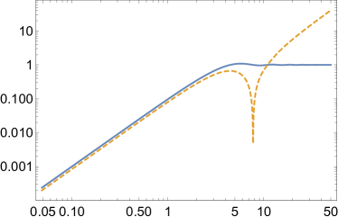
Again, the kernel is a function of only kη𝑘𝜂k\eta. The reason why we have such a simple kernel for the scalar-scalar source is because the scalar perturbations can be written in terms of the constant {\cal R}, so the time integral is greatly simplified. These scalar-scalar induced solutions in the zero-shear gauge (55) and comoving gauge (57) agree with Hwang et al. (2017). In Figure 1, we show the kernels barring the factor 6/5. As kη𝑘𝜂k\eta becomes bigger, the zero-shear gauge kernel approaches 1 while that in the comoving gauge increases as (kη)2superscript𝑘𝜂2(k\eta)^{2}. Thus on small scales the amplitude of the induced GWs in the comoving gauge is much bigger than that in the zero-shear gauge. This shows clearly the gauge dependence of the scalar-induced GWs.
Refer to caption
Figure 1: The kernels for the scalar-scalar induced GWs during MD in the zero-shear gauge (55) (solid line) and comoving gauge (57) (dashed line) as a function of kη𝑘𝜂k\eta.

4.3 Scalar-tensor induced GWs during MD

Next we consider the GWs induced by the scalar-tensor source during MD. Considering first the zero-shear gauge in which χ=0𝜒0\chi=0 and α=φ𝛼𝜑\alpha=-\varphi, we find (omitting the subscript χ𝜒\chi for the scalar perturbation φ𝜑\varphi)

sij(st)(𝒌)superscriptsubscript𝑠𝑖𝑗𝑠𝑡𝒌\displaystyle s_{ij}^{(st)}({\bm{k}}) =d3q1d3q2(2π)3δ(3)(𝒌𝒒12)12[(ddt+3H)(φ1h˙λ2+2φ˙1hλ2)φ1ddt(h˙λ2)+κ1h˙λ2+2a2(2kkq2k+q12)φ1hλ2]eij2λabsentsuperscript𝑑3subscript𝑞1superscript𝑑3subscript𝑞2superscript2𝜋3superscript𝛿3𝒌subscript𝒒1212delimited-[]𝑑𝑑𝑡3𝐻subscript𝜑1subscript˙superscript𝜆22subscript˙𝜑1subscriptsuperscript𝜆2subscript𝜑1𝑑𝑑𝑡subscript˙superscript𝜆2subscript𝜅1subscript˙superscript𝜆22superscript𝑎22superscript𝑘𝑘subscript𝑞2𝑘superscriptsubscript𝑞12subscript𝜑1subscriptsuperscript𝜆2superscriptsubscript𝑒𝑖𝑗2superscript𝜆\displaystyle=\int\frac{d^{3}q_{1}d^{3}q_{2}}{(2\pi)^{3}}\delta^{(3)}({\bm{k}}-{\bm{q}}_{12})\frac{1}{2}\bigg{[}\bigg{(}\frac{d}{dt}+3H\bigg{)}\Big{(}\varphi_{1}\dot{h}_{\lambda^{\prime}2}+2\dot{\varphi}_{1}h_{\lambda^{\prime}2}\Big{)}-\varphi_{1}\frac{d}{dt}\Big{(}\dot{h}_{\lambda^{\prime}2}\Big{)}+\kappa_{1}\dot{h}_{\lambda^{\prime}2}+\frac{2}{a^{2}}\Big{(}2k^{k}q_{2k}+q_{1}^{2}\Big{)}\varphi_{1}h_{\lambda^{\prime}2}\bigg{]}e_{ij2}^{\lambda^{\prime}}
+(𝒒1𝒒2),\displaystyle\quad+({\bm{q}}_{1}\leftrightarrow{\bm{q}}_{2})\,, (58)

where the subscript 1 for a perturbation variable means it is a function of 𝒒1subscript𝒒1{\bm{q}}_{1}, e.g. φ1=φ(𝒒1)subscript𝜑1𝜑subscript𝒒1\varphi_{1}=\varphi({\bm{q}}_{1}) and so on. Using φχ=3/5subscript𝜑𝜒35\varphi_{\chi}=3{\cal R}/5 and κχ=9H/5subscript𝜅𝜒9𝐻5\kappa_{\chi}=-9H{\cal R}/5 during MD with {\cal R} = constant, the terms including the time derivative of the linear tensor perturbation vanish and we have the following simple expression for the source:

eλij(𝒌)sij(st)(𝒌)=1a265d3q(2π)3[eλij(𝒌)eijλ(𝒒)](k2+q2)(𝒌𝒒)hλ(η,𝒒).subscriptsuperscript𝑒𝑖𝑗𝜆𝒌superscriptsubscript𝑠𝑖𝑗𝑠𝑡𝒌1superscript𝑎265superscript𝑑3𝑞superscript2𝜋3delimited-[]subscriptsuperscript𝑒𝑖𝑗𝜆𝒌superscriptsubscript𝑒𝑖𝑗superscript𝜆𝒒superscript𝑘2superscript𝑞2𝒌𝒒subscriptsuperscript𝜆𝜂𝒒e^{ij}_{\lambda}({\bm{k}})s_{ij}^{(st)}({\bm{k}})=\frac{1}{a^{2}}\frac{6}{5}\int\frac{d^{3}q}{(2\pi)^{3}}\big{[}e^{ij}_{\lambda}({\bm{k}})e_{ij}^{\lambda^{\prime}}({\bm{q}})\big{]}\big{(}k^{2}+q^{2}\big{)}{\cal R}({\bm{k}}-{\bm{q}})h_{\lambda^{\prime}}(\eta,{\bm{q}})\,. (59)

It is very important to note that the linear order perturbation hλsubscriptsuperscript𝜆h_{\lambda^{\prime}} does possess time dependence as given by (39). Thus, unlike the scalar-scalar source case, the time integral for the Green’s function solution includes another time-dependent function from hλsubscriptsuperscript𝜆h_{\lambda^{\prime}}, namely, j1(kη)/(kη)subscript𝑗1𝑘𝜂𝑘𝜂j_{1}(k\eta)/(k\eta):

hλ(η,𝒌)subscript𝜆𝜂𝒌\displaystyle h_{\lambda}(\eta,{\bm{k}}) =185d3q(2π)3[eλij(𝒌)eijλ(𝒒)](q2+k2)(𝒌𝒒)h0λ(𝒒)1kqx[y1(x)0x𝑑x~x~2j1(qkx~)j1(x~)j1(x)0x𝑑x~x~2j1(qkx~)y1(x~)]absent185superscript𝑑3𝑞superscript2𝜋3delimited-[]subscriptsuperscript𝑒𝑖𝑗𝜆𝒌superscriptsubscript𝑒𝑖𝑗superscript𝜆𝒒superscript𝑞2superscript𝑘2𝒌𝒒superscriptsubscript0superscript𝜆𝒒1𝑘𝑞𝑥delimited-[]subscript𝑦1𝑥superscriptsubscript0𝑥differential-d~𝑥superscript~𝑥2subscript𝑗1𝑞𝑘~𝑥subscript𝑗1~𝑥subscript𝑗1𝑥superscriptsubscript0𝑥differential-d~𝑥superscript~𝑥2subscript𝑗1𝑞𝑘~𝑥subscript𝑦1~𝑥\displaystyle=\frac{18}{5}\int\frac{d^{3}q}{(2\pi)^{3}}\big{[}e^{ij}_{\lambda}({\bm{k}})e_{ij}^{\lambda^{\prime}}({\bm{q}})\big{]}\big{(}q^{2}+k^{2}\big{)}{\cal R}({\bm{k}}-{\bm{q}})h_{0}^{\lambda^{\prime}}({\bm{q}})\frac{1}{kqx}\bigg{[}y_{1}(x)\int_{0}^{x}d\tilde{x}\tilde{x}^{2}j_{1}\bigg{(}\frac{q}{k}\tilde{x}\bigg{)}j_{1}(\tilde{x})-j_{1}(x)\int_{0}^{x}d\tilde{x}\tilde{x}^{2}j_{1}\bigg{(}\frac{q}{k}\tilde{x}\bigg{)}y_{1}(\tilde{x})\bigg{]}
=185d3q(2π)3[eλij(𝒌)eijλ(𝒒)](𝒌𝒒)h0λ(𝒒)[j1(kη)kηj1(qη)qη]q2+k2q2k2.absent185superscript𝑑3𝑞superscript2𝜋3delimited-[]subscriptsuperscript𝑒𝑖𝑗𝜆𝒌superscriptsubscript𝑒𝑖𝑗superscript𝜆𝒒𝒌𝒒superscriptsubscript0superscript𝜆𝒒delimited-[]subscript𝑗1𝑘𝜂𝑘𝜂subscript𝑗1𝑞𝜂𝑞𝜂superscript𝑞2superscript𝑘2superscript𝑞2superscript𝑘2\displaystyle=\frac{18}{5}\int\frac{d^{3}q}{(2\pi)^{3}}\big{[}e^{ij}_{\lambda}({\bm{k}})e_{ij}^{\lambda^{\prime}}({\bm{q}})\big{]}{\cal R}({\bm{k}}-{\bm{q}})h_{0}^{\lambda^{\prime}}({\bm{q}})\bigg{[}\frac{j_{1}(k\eta)}{k\eta}-\frac{j_{1}(q\eta)}{q\eta}\bigg{]}\frac{q^{2}+k^{2}}{q^{2}-k^{2}}\,. (60)

The detail of the x~~𝑥\tilde{x}-integrals is given in Appendix B.1.

In the comoving gauge where v=0𝑣0v=0, using =absent{\cal R}= constant and

ddt(1a2H)=12a2,𝑑𝑑𝑡1superscript𝑎2𝐻12superscript𝑎2\frac{d}{dt}\bigg{(}\frac{1}{a^{2}H}\bigg{)}=-\frac{1}{2a^{2}}\,, (61)

which follows from H=2/(3t)𝐻23𝑡H=2/(3t) during MD, straightforward calculations give

eλij(𝒌)sij(st)(𝒌)=2a2d3q(2π)3[eλij(𝒌)eijλ(𝒒)](𝒌𝒒)[15H(k2q2)h˙λ(𝒒)+k2hλ(𝒒)].subscriptsuperscript𝑒𝑖𝑗𝜆𝒌superscriptsubscript𝑠𝑖𝑗𝑠𝑡𝒌2superscript𝑎2superscript𝑑3𝑞superscript2𝜋3delimited-[]subscriptsuperscript𝑒𝑖𝑗𝜆𝒌subscriptsuperscript𝑒superscript𝜆𝑖𝑗𝒒𝒌𝒒delimited-[]15𝐻superscript𝑘2superscript𝑞2subscript˙superscript𝜆𝒒superscript𝑘2subscriptsuperscript𝜆𝒒e^{ij}_{\lambda}({\bm{k}})s_{ij}^{(st)}({\bm{k}})=\frac{2}{a^{2}}\int\frac{d^{3}q}{(2\pi)^{3}}\big{[}e^{ij}_{\lambda}({\bm{k}})e^{\lambda^{\prime}}_{ij}({\bm{q}})\big{]}{\cal R}({\bm{k}}-{\bm{q}})\bigg{[}\frac{1}{5H}\big{(}k^{2}-q^{2}\big{)}\dot{h}_{\lambda^{\prime}}({\bm{q}})+k^{2}{h}_{\lambda^{\prime}}({\bm{q}})\bigg{]}\,. (62)

Unlike the zero-shear gauge case, the time derivative of the linear tensor perturbation remains, which is given by

h˙λ(𝒒)=qadd(qη)hλ(η,𝒒)=qa3h0λ(𝒒)[3j1(qη)(qη)2+j0(qη)qη].subscript˙superscript𝜆𝒒𝑞𝑎𝑑𝑑𝑞𝜂subscriptsuperscript𝜆𝜂𝒒𝑞𝑎3superscriptsubscript0superscript𝜆𝒒delimited-[]3subscript𝑗1𝑞𝜂superscript𝑞𝜂2subscript𝑗0𝑞𝜂𝑞𝜂\displaystyle\dot{h}_{\lambda^{\prime}}({\bm{q}})=\frac{q}{a}\frac{d}{d(q\eta)}h_{\lambda^{\prime}}(\eta,{\bm{q}})=\frac{q}{a}3h_{0}^{\lambda^{\prime}}({\bm{q}})\bigg{[}-3\frac{j_{1}(q\eta)}{(q\eta)^{2}}+\frac{j_{0}(q\eta)}{q\eta}\bigg{]}\,. (63)

We can find the solution in a manner very similar to (4.3) but with different sij(st)superscriptsubscript𝑠𝑖𝑗𝑠𝑡s_{ij}^{(st)} as:

hλ(η,𝒌)subscript𝜆𝜂𝒌\displaystyle h_{\lambda}(\eta,{\bm{k}}) =6k2xd3q(2π)3[eλij(𝒌)eijλ(𝒒)](𝒌𝒒)h0λ(𝒒)0x𝑑x~x~3[3q2+7k210j1(qx~/k)qx~/k+k2q210j0(qkx~)]absent6superscript𝑘2𝑥superscript𝑑3𝑞superscript2𝜋3delimited-[]subscriptsuperscript𝑒𝑖𝑗𝜆𝒌superscriptsubscript𝑒𝑖𝑗superscript𝜆𝒒𝒌𝒒superscriptsubscript0superscript𝜆𝒒superscriptsubscript0𝑥differential-d~𝑥superscript~𝑥3delimited-[]3superscript𝑞27superscript𝑘210subscript𝑗1𝑞~𝑥𝑘𝑞~𝑥𝑘superscript𝑘2superscript𝑞210subscript𝑗0𝑞𝑘~𝑥\displaystyle=\frac{6}{k^{2}x}\int\frac{d^{3}q}{(2\pi)^{3}}\big{[}e^{ij}_{\lambda}({\bm{k}})e_{ij}^{\lambda^{\prime}}({\bm{q}})\big{]}{\cal R}({\bm{k}}-{\bm{q}})h_{0}^{\lambda^{\prime}}({\bm{q}})\int_{0}^{x}d\tilde{x}\tilde{x}^{3}\bigg{[}\frac{3q^{2}+7k^{2}}{10}\frac{j_{1}(q\tilde{x}/k)}{q\tilde{x}/k}+\frac{k^{2}-q^{2}}{10}j_{0}\bigg{(}\frac{q}{k}\tilde{x}\bigg{)}\bigg{]}
×[j1(x~)y1(x)j1(x)y1(x~)]absentdelimited-[]subscript𝑗1~𝑥subscript𝑦1𝑥subscript𝑗1𝑥subscript𝑦1~𝑥\displaystyle\quad\times\Big{[}j_{1}(\tilde{x})y_{1}(x)-j_{1}(x)y_{1}(\tilde{x})\Big{]}
=6d3q(2π)3[eλij(𝒌)eijλ(𝒒)](𝒌𝒒)h0λ(𝒒)[q2+5k25(q2k2)j1(kη)kη5q2+7k210(q2k2)j1(qη)qη+110j0(qη)].absent6superscript𝑑3𝑞superscript2𝜋3delimited-[]subscriptsuperscript𝑒𝑖𝑗𝜆𝒌superscriptsubscript𝑒𝑖𝑗superscript𝜆𝒒𝒌𝒒superscriptsubscript0superscript𝜆𝒒delimited-[]superscript𝑞25superscript𝑘25superscript𝑞2superscript𝑘2subscript𝑗1𝑘𝜂𝑘𝜂5superscript𝑞27superscript𝑘210superscript𝑞2superscript𝑘2subscript𝑗1𝑞𝜂𝑞𝜂110subscript𝑗0𝑞𝜂\displaystyle=6\int\frac{d^{3}q}{(2\pi)^{3}}\big{[}e^{ij}_{\lambda}({\bm{k}})e_{ij}^{\lambda^{\prime}}({\bm{q}})\big{]}{\cal R}({\bm{k}}-{\bm{q}})h_{0}^{\lambda^{\prime}}({\bm{q}})\bigg{[}\frac{q^{2}+5k^{2}}{5(q^{2}-k^{2})}\frac{j_{1}(k\eta)}{k\eta}-\frac{5q^{2}+7k^{2}}{10(q^{2}-k^{2})}\frac{j_{1}(q\eta)}{q\eta}+\frac{1}{10}j_{0}(q\eta)\bigg{]}\,. (64)

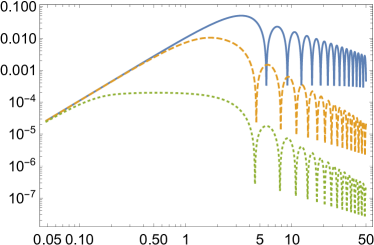
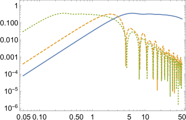
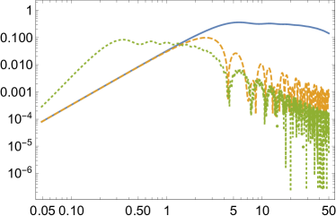
This is the solution of the induced hλ(𝒌,η)subscript𝜆𝒌𝜂h_{\lambda}({\bm{k}},\eta) from the scalar-tensor source in the comoving gauge. In Figure 2 we show the kernels in both gauges. For kη1greater-than-or-equivalent-to𝑘𝜂1k\eta\gtrsim 1 with sizeable q/k𝑞𝑘q/k, the comoving gauge kernel exhibits more rapid oscillations. But for small q/k𝑞𝑘q/k, both kernels are approximated by 1/3j1(kη)/(kη)+𝒪(q2/k2)13subscript𝑗1𝑘𝜂𝑘𝜂𝒪superscript𝑞2superscript𝑘21/3-j_{1}(k\eta)/(k\eta)+{\cal O}(q^{2}/k^{2}) so they behave similarly. Compared to the scalar-scalar induced GWs as we have seen previously, the difference in the zero-shear gauge and comoving gauge is not prominent. This is because the gradient of the shear, that gives rise to the huge difference on small scales for the scalar-scalar induced GWs, is highly suppressed by the exponentially decaying linear GWs on small scales.
Refer to caption
Refer to caption
Figure 2: The kernels in the (left) zero-shear gauge and (right) comoving gauge as a function of kη𝑘𝜂k\eta. Since the kernels are also dependent on q𝑞q, we set (solid lines) q/k=0.05𝑞𝑘0.05q/k=0.05, (dashed lines) q/k=2𝑞𝑘2q/k=2 and (dotted lines) q/k=20𝑞𝑘20q/k=20 in both panels.

4.4 Tensor-tensor induced GWs during MD

Next we consider the tensor-tensor source during MD. Multiplying the polarization tensor eλij(𝒌)subscriptsuperscript𝑒𝑖𝑗𝜆𝒌e^{ij}_{\lambda}({\bm{k}}) and separating the time-dependent part gives

eλij(𝒌)sij(tt)(𝒌)subscriptsuperscript𝑒𝑖𝑗𝜆𝒌superscriptsubscript𝑠𝑖𝑗𝑡𝑡𝒌\displaystyle e^{ij}_{\lambda}({\bm{k}})s_{ij}^{(tt)}({\bm{k}}) =1a2d3q1d3q2(2π)3δ(3)(𝒌𝒒12){9h0λ1(𝒒1)h0λ2(𝒒2)eλij(𝒌)ei1kλ1ejk2λ2𝒞λ(𝒒1,𝒒2)q1q2[3j1(q1η)(q1η)2+j0(q1η)q1η][3j1(q2η)(q2η)2+j0(q2η)q2η]\displaystyle=\frac{1}{a^{2}}\int\frac{d^{3}q_{1}d^{3}q_{2}}{(2\pi)^{3}}\delta^{(3)}({\bm{k}}-{\bm{q}}_{12})\bigg{\{}\underbrace{9h_{0}^{\lambda_{1}}({\bm{q}}_{1})h_{0}^{\lambda_{2}}({\bm{q}}_{2})e^{ij}_{\lambda}({\bm{k}})e_{i1}^{k\lambda_{1}}e_{jk2}^{\lambda_{2}}}_{\equiv{\cal C}_{\lambda}({\bm{q}}_{1},{\bm{q}}_{2})}q_{1}q_{2}\bigg{[}-3\frac{j_{1}(q_{1}\eta)}{(q_{1}\eta)^{2}}+\frac{j_{0}(q_{1}\eta)}{q_{1}\eta}\bigg{]}\bigg{[}-3\frac{j_{1}(q_{2}\eta)}{(q_{2}\eta)^{2}}+\frac{j_{0}(q_{2}\eta)}{q_{2}\eta}\bigg{]}
+9h0λ1(𝒒1)h0λ2(𝒒2)eλij(𝒌)[eλ11kl(q2jq2keil2λ2q2iq2kejl2λ2+q2kq2leij2λ2)\displaystyle\hskip 100.00015pt+9h_{0}^{\lambda_{1}}({\bm{q}}_{1})h_{0}^{\lambda_{2}}({\bm{q}}_{2})e^{ij}_{\lambda}({\bm{k}})\bigg{[}e^{kl}_{\lambda_{1}1}\big{(}-q_{2j}q_{2k}e^{\lambda_{2}}_{il2}-q_{2i}q_{2k}e_{jl2}^{\lambda_{2}}+q_{2k}q_{2l}e^{\lambda_{2}}_{ij2}\big{)}
+12q1iq1jeλ1kl1ekl2λ2+(𝒒1𝒒2)ei1kλ1ejk2λ2q1lq2kei1kλ1ejl2λ2]𝒟λ(𝒒1,𝒒2)j1(q1η)q1ηj1(q2η)q2η}\displaystyle\hskip 110.00017pt\underbrace{\hskip 100.00015pt+\frac{1}{2}q_{1i}q_{1j}e_{\lambda_{1}}^{kl1}e_{kl2}^{\lambda_{2}}+({\bm{q}}_{1}\cdot{\bm{q}}_{2})e_{i1}^{k\lambda_{1}}e_{jk2}^{\lambda_{2}}-q_{1}^{l}q_{2k}e_{i1}^{k\lambda_{1}}e_{jl2}^{\lambda_{2}}\bigg{]}}_{\equiv{\cal D}_{\lambda}({\bm{q}}_{1},{\bm{q}}_{2})}\frac{j_{1}(q_{1}\eta)}{q_{1}\eta}\frac{j_{1}(q_{2}\eta)}{q_{2}\eta}\bigg{\}}
+(𝒒1𝒒2).\displaystyle\quad+({\bm{q}}_{1}\leftrightarrow{\bm{q}}_{2})\,. (65)

As can be seen, only the Bessel function terms contain time dependence. Then the solution for hλsubscript𝜆h_{\lambda} can be written as

hλ(η,𝒌)subscript𝜆𝜂𝒌\displaystyle h_{\lambda}(\eta,{\bm{k}}) =d3q1d3q2(2π)3δ(3)(𝒌𝒒12){[𝒞λ(𝒒1,𝒒2)+(𝒒1𝒒2)]q¯1q¯2x[9q¯12q¯220xdx~x~1j1(q¯1x~)j1(q¯1x~)3q¯12q¯20xdx~j1(q¯1x~)j0(q¯2x~)\displaystyle=\int\frac{d^{3}q_{1}d^{3}q_{2}}{(2\pi)^{3}}\delta^{(3)}({\bm{k}}-{\bm{q}}_{12})\Bigg{\{}\Big{[}{\cal C}_{\lambda}({\bm{q}}_{1},{\bm{q}}_{2})+({\bm{q}}_{1}\leftrightarrow{\bm{q}}_{2})\Big{]}\frac{\bar{q}_{1}\bar{q}_{2}}{x}\bigg{[}\frac{9}{\bar{q}_{1}^{2}\bar{q}_{2}^{2}}\int_{0}^{x}d\tilde{x}\tilde{x}^{-1}j_{1}(\bar{q}_{1}\tilde{x})j_{1}(\bar{q}_{1}\tilde{x})-\frac{3}{\bar{q}_{1}^{2}\bar{q}_{2}}\int_{0}^{x}d\tilde{x}j_{1}(\bar{q}_{1}\tilde{x})j_{0}(\bar{q}_{2}\tilde{x})
3q¯1q¯220xdx~j0(q¯1x~)j1(q¯2x~)+1q¯1q¯20xdx~x~j0(q¯1x~)j0(q¯2x~)][j1(x~)y1(x)j1(x)y1(x~)]\displaystyle\hskip 140.00021pt-\frac{3}{\bar{q}_{1}\bar{q}_{2}^{2}}\int_{0}^{x}d\tilde{x}j_{0}(\bar{q}_{1}\tilde{x})j_{1}(\bar{q}_{2}\tilde{x})+\frac{1}{\bar{q}_{1}\bar{q}_{2}}\int_{0}^{x}d\tilde{x}\tilde{x}j_{0}(\bar{q}_{1}\tilde{x})j_{0}(\bar{q}_{2}\tilde{x})\bigg{]}\Big{[}j_{1}(\tilde{x})y_{1}(x)-j_{1}(x)y_{1}(\tilde{x})\Big{]}
+[𝒟λ(𝒒1,𝒒2)+(𝒒1𝒒2)]1k2x1q¯1q¯20xdx~x~j1(q¯1x~)j1(q¯1x~)[j1(x~)y1(x)j1(x)y1(x~)]},\displaystyle\hskip 100.00015pt+\Big{[}{\cal D}_{\lambda}({\bm{q}}_{1},{\bm{q}}_{2})+({\bm{q}}_{1}\leftrightarrow{\bm{q}}_{2})\Big{]}\frac{1}{k^{2}x}\frac{1}{\bar{q}_{1}\bar{q}_{2}}\int_{0}^{x}d\tilde{x}\tilde{x}j_{1}(\bar{q}_{1}\tilde{x})j_{1}(\bar{q}_{1}\tilde{x})\Big{[}j_{1}(\tilde{x})y_{1}(x)-j_{1}(x)y_{1}(\tilde{x})\Big{]}\Bigg{\}}\,, (66)

where q¯1q1/ksubscript¯𝑞1subscript𝑞1𝑘\bar{q}_{1}\equiv q_{1}/k and q¯2q2/ksubscript¯𝑞2subscript𝑞2𝑘\bar{q}_{2}\equiv q_{2}/k respectively.

Now, using the recurrence relation (B.4) for n=1𝑛1n=1, we find

j2(q¯2x)=3q¯2xj1(q¯1x)j0(q¯1x)=3q¯2[j1(q¯2x)xq¯23j0(q¯2x)],subscript𝑗2subscript¯𝑞2𝑥3subscript¯𝑞2𝑥subscript𝑗1subscript¯𝑞1𝑥subscript𝑗0subscript¯𝑞1𝑥3subscript¯𝑞2delimited-[]subscript𝑗1subscript¯𝑞2𝑥𝑥subscript¯𝑞23subscript𝑗0subscript¯𝑞2𝑥j_{2}(\bar{q}_{2}x)=\frac{3}{\bar{q}_{2}x}j_{1}(\bar{q}_{1}x)-j_{0}(\bar{q}_{1}x)=\frac{3}{\bar{q}_{2}}\bigg{[}\frac{j_{1}(\bar{q}_{2}x)}{x}-\frac{\bar{q}_{2}}{3}j_{0}(\bar{q}_{2}x)\bigg{]}\,, (67)

so that the terms multiplied by 𝒞λ(𝒒1,𝒒2)subscript𝒞𝜆subscript𝒒1subscript𝒒2{\cal C}_{\lambda}({\bm{q}}_{1},{\bm{q}}_{2}) become very simple as

[9q¯12q¯220x𝑑x~x~1j1(q¯1x~)j1(q¯2x~)3q¯12q¯20x𝑑x~j1(q¯1x~)j0(q¯2x~)3q¯1q¯220x𝑑x~j0(q¯1x~)j1(q¯2x~)+1q¯1q¯20x𝑑x~x~j0(q¯1x~)j0(q¯2x~)]f1(x~)delimited-[]9superscriptsubscript¯𝑞12superscriptsubscript¯𝑞22superscriptsubscript0𝑥differential-d~𝑥superscript~𝑥1subscript𝑗1subscript¯𝑞1~𝑥subscript𝑗1subscript¯𝑞2~𝑥3superscriptsubscript¯𝑞12subscript¯𝑞2superscriptsubscript0𝑥differential-d~𝑥subscript𝑗1subscript¯𝑞1~𝑥subscript𝑗0subscript¯𝑞2~𝑥3subscript¯𝑞1superscriptsubscript¯𝑞22superscriptsubscript0𝑥differential-d~𝑥subscript𝑗0subscript¯𝑞1~𝑥subscript𝑗1subscript¯𝑞2~𝑥1subscript¯𝑞1subscript¯𝑞2superscriptsubscript0𝑥differential-d~𝑥~𝑥subscript𝑗0subscript¯𝑞1~𝑥subscript𝑗0subscript¯𝑞2~𝑥subscript𝑓1~𝑥\displaystyle\bigg{[}\frac{9}{\bar{q}_{1}^{2}\bar{q}_{2}^{2}}\int_{0}^{x}d\tilde{x}\tilde{x}^{-1}j_{1}(\bar{q}_{1}\tilde{x})j_{1}(\bar{q}_{2}\tilde{x})-\frac{3}{\bar{q}_{1}^{2}\bar{q}_{2}}\int_{0}^{x}d\tilde{x}j_{1}(\bar{q}_{1}\tilde{x})j_{0}(\bar{q}_{2}\tilde{x})-\frac{3}{\bar{q}_{1}\bar{q}_{2}^{2}}\int_{0}^{x}d\tilde{x}j_{0}(\bar{q}_{1}\tilde{x})j_{1}(\bar{q}_{2}\tilde{x})+\frac{1}{\bar{q}_{1}\bar{q}_{2}}\int_{0}^{x}d\tilde{x}\tilde{x}j_{0}(\bar{q}_{1}\tilde{x})j_{0}(\bar{q}_{2}\tilde{x})\bigg{]}f_{1}(\tilde{x})
=1q¯1q¯20x𝑑x~x~j2(q¯1x~)j2(q¯2x~)f1(x~),absent1subscript¯𝑞1subscript¯𝑞2superscriptsubscript0𝑥differential-d~𝑥~𝑥subscript𝑗2subscript¯𝑞1~𝑥subscript𝑗2subscript¯𝑞2~𝑥subscript𝑓1~𝑥\displaystyle=\frac{1}{\bar{q}_{1}\bar{q}_{2}}\int_{0}^{x}d\tilde{x}\tilde{x}j_{2}(\bar{q}_{1}\tilde{x})j_{2}(\bar{q}_{2}\tilde{x})f_{1}(\tilde{x})\,, (68)

where f1(x~)subscript𝑓1~𝑥f_{1}(\tilde{x}) denotes both first- and second-kind of the spherical Bessel functions. Since limx0y1(x)=1/x21/2+subscript𝑥0subscript𝑦1𝑥1superscript𝑥212\lim_{x\to 0}y_{1}(x)=-1/x^{2}-1/2+\cdots and limx0jn(x)xnsimilar-tosubscript𝑥0subscript𝑗𝑛𝑥superscript𝑥𝑛\lim_{x\to 0}j_{n}(x)\sim x^{n}, we always have converging results. Thus, we can write (4.4) as

hλ(η,𝒌)subscript𝜆𝜂𝒌\displaystyle h_{\lambda}(\eta,{\bm{k}}) =d3q1d3q2(2π)3δ(3)(𝒌𝒒12){[𝒞λ(𝒒1,𝒒2)+(𝒒1𝒒2)]1x0xdx~x~j2(q¯1x~)j2(q¯2x~)[j1(x~)y1(x)j1(x)y1(x~)]\displaystyle=\int\frac{d^{3}q_{1}d^{3}q_{2}}{(2\pi)^{3}}\delta^{(3)}({\bm{k}}-{\bm{q}}_{12})\bigg{\{}\Big{[}{\cal C}_{\lambda}({\bm{q}}_{1},{\bm{q}}_{2})+({\bm{q}}_{1}\leftrightarrow{\bm{q}}_{2})\Big{]}\frac{1}{x}\int_{0}^{x}d\tilde{x}\tilde{x}j_{2}(\bar{q}_{1}\tilde{x})j_{2}(\bar{q}_{2}\tilde{x})\Big{[}j_{1}(\tilde{x})y_{1}(x)-j_{1}(x)y_{1}(\tilde{x})\Big{]}
+1k2[𝒟λ(𝒒1,𝒒2)+(𝒒1𝒒2)]1q¯1q¯2x0xdx~x~j1(q¯1x~)j1(q¯2x~)[j1(x~)y1(x)j1(x)y1(x~)]}.\displaystyle\hskip 120.00018pt+\frac{1}{k^{2}}\Big{[}{\cal D}_{\lambda}({\bm{q}}_{1},{\bm{q}}_{2})+({\bm{q}}_{1}\leftrightarrow{\bm{q}}_{2})\Big{]}\frac{1}{\bar{q}_{1}\bar{q}_{2}x}\int_{0}^{x}d\tilde{x}\tilde{x}j_{1}(\bar{q}_{1}\tilde{x})j_{1}(\bar{q}_{2}\tilde{x})\Big{[}j_{1}(\tilde{x})y_{1}(x)-j_{1}(x)y_{1}(\tilde{x})\Big{]}\bigg{\}}\,. (69)

Both the x~~𝑥\tilde{x} integrals can be performed analytically, with the details given in Appendix B.2. Performing the momentum integral using the delta function, finally (4.4) becomes

hλ(η,𝒌)subscript𝜆𝜂𝒌\displaystyle h_{\lambda}(\eta,{\bm{k}}) =d3q(2π)318h0λ1(𝒒)h0λ2(𝒌𝒒){eλij(𝒌)eikλ1(𝒒)ejkλ2(𝒌𝒒)FMD(𝒌,𝒒,η)\displaystyle=\int\frac{d^{3}q}{(2\pi)^{3}}18h_{0}^{\lambda_{1}}({\bm{q}})h_{0}^{\lambda_{2}}({\bm{k}}-{\bm{q}})\Bigg{\{}e_{\lambda}^{ij}({\bm{k}})e_{i}^{k\lambda_{1}}({\bm{q}})e_{jk}^{\lambda_{2}}({\bm{k}}-{\bm{q}})F_{\text{MD}}({\bm{k}},{\bm{q}},\eta)
+1k2(eλij(𝒌)eλ1kl(𝒒)(qjkkeilλ2(𝒌𝒒)+qikkejlλ2(𝒌𝒒)+kkkleijλ2(𝒌𝒒))\displaystyle\hskip 15.00002pt+\frac{1}{k^{2}}\bigg{(}e_{\lambda}^{ij}({\bm{k}})e^{kl}_{\lambda_{1}}({\bm{q}})\Big{(}q_{j}k_{k}e_{il}^{\lambda_{2}}({\bm{k}}-{\bm{q}})+q_{i}k_{k}e_{jl}^{\lambda_{2}}({\bm{k}}-{\bm{q}})+k_{k}k_{l}e_{ij}^{\lambda_{2}}({\bm{k}}-{\bm{q}})\Big{)}
+eλij(𝒌)[12qiqjeλ1kl(𝒒)eklλ2(𝒌𝒒)+𝒒(𝒌𝒒)eikλ1(𝒒)ejkλ2(𝒌𝒒)qlkkeikλ1(𝒒)ejlλ2(𝒌𝒒)])GMD(𝒌,𝒒,η)},\displaystyle\hskip 20.00003pt+e_{\lambda}^{ij}({\bm{k}})\bigg{[}\frac{1}{2}q_{i}q_{j}e^{kl}_{\lambda_{1}}({\bm{q}})e_{kl}^{\lambda_{2}}({\bm{k}}-{\bm{q}})+{\bm{q}}\cdot({\bm{k}}-{\bm{q}})e_{i}^{k\lambda_{1}}({\bm{q}})e_{jk}^{\lambda_{2}}({\bm{k}}-{\bm{q}})-q^{l}k_{k}e_{i}^{k\lambda_{1}}({\bm{q}})e_{jl}^{\lambda_{2}}({\bm{k}}-{\bm{q}})\bigg{]}\bigg{)}G_{\text{MD}}({\bm{k}},{\bm{q}},\eta)\Bigg{\}}\,, (70)

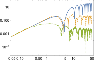
where the kernels FMDsubscript𝐹MDF_{\text{MD}} and GMDsubscript𝐺MDG_{\text{MD}} are given respectively by (B.2) and (B.2). In Figure 3 we show FMDsubscript𝐹MDF_{\text{MD}} and GMDsubscript𝐺MDG_{\text{MD}}.

Refer to caption
Refer to caption
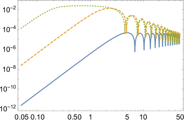
Figure 3: The kernels (left) FMDsubscript𝐹MDF_{\text{MD}} and (right) GMDsubscript𝐺MDG_{\text{MD}} as a function of kη𝑘𝜂k\eta. Since they are also dependent on the angle between 𝒌𝒌{\bm{k}} and 𝒒𝒒{\bm{q}}, for simplicity we set in such a way that for both (solid lines) q/k=0.05𝑞𝑘0.05q/k=0.05 and (dotted lines) q/k=20𝑞𝑘20q/k=20 they are aligned perpendicularly, i.e. cos(𝒌^𝒒^)=0^𝒌^𝒒0\cos\big{(}\hat{\bm{k}}\cdot\hat{\bm{q}}\big{)}=0, while for (dashed lines) q/k=2𝑞𝑘2q/k=2 the angle between them is 2π/32𝜋32\pi/3, cos(𝒌^𝒒^)=1/2^𝒌^𝒒12\cos\big{(}\hat{\bm{k}}\cdot\hat{\bm{q}}\big{)}=-1/2 in both panels.

4.5 Scalar-scalar induced GWs during RD

Until now we have considered the second-order solutions for the induced GWs during MD. Now we consider the solutions during RD. Especially, after the first version of the present work appeared in arXiv, there have been a number of papers published in the literature, e.g. De Luca et al. (2020); Inomata & Terada (2020); Yuan et al. (2020), claiming that the gauge dependence of the induced GWs during RD disappears. This is not the case, at least regarding the solutions in the two gauge conditions we examine here explicitly – the zero-shear gauge and comoving gauge: the solutions are clearly different in these two gauges as can be seen in (4.5) and (4.5) [see also Tomikawa & Kobayashi (2020)].

An important difference for the linear solutions for the scalar perturbations is that now the curvature perturbation φ𝜑\varphi does not stay constant, but decays once the mode enters the horizon. Thus, the scalar-scalar induced GWs during RD do not behave simply as we have seen during MD, but exhibit rapid oscillations. We first consider the zero-shear gauge, in which the scalar-scalar source reads rather simply as

sij(ss)(𝒌)=d3q(2π)3[2a2qiqjφχ(𝒒)φχ(𝒌𝒒)+8πG(ρ+p)qiqjvχ(𝒒)vχ(𝒌𝒒)].superscriptsubscript𝑠𝑖𝑗𝑠𝑠𝒌superscript𝑑3𝑞superscript2𝜋3delimited-[]2superscript𝑎2subscript𝑞𝑖subscript𝑞𝑗subscript𝜑𝜒𝒒subscript𝜑𝜒𝒌𝒒8𝜋𝐺𝜌𝑝subscript𝑞𝑖subscript𝑞𝑗subscript𝑣𝜒𝒒subscript𝑣𝜒𝒌𝒒s_{ij}^{(ss)}(\bm{k})=\int\frac{d^{3}q}{(2\pi)^{3}}\bigg{[}\frac{2}{a^{2}}q_{i}q_{j}\varphi_{\chi}(\bm{q})\varphi_{\chi}(\bm{k}-\bm{q})+8\pi G(\rho+p)q_{i}q_{j}v_{\chi}(\bm{q})v_{\chi}(\bm{k}-\bm{q})\bigg{]}\,. (71)

With the scalar solutions given by (29) and defining

qη3=q3kkηq¯1xand|𝒌𝒒|η3=|𝒌𝒒|3kkηq¯2x,formulae-sequence𝑞𝜂3𝑞3𝑘𝑘𝜂subscript¯𝑞1𝑥and𝒌𝒒𝜂3𝒌𝒒3𝑘𝑘𝜂subscript¯𝑞2𝑥\frac{q\eta}{\sqrt{3}}=\frac{q}{\sqrt{3}k}k\eta\equiv\bar{q}_{1}x\quad\text{and}\quad\frac{|{\bm{k}}-{\bm{q}}|\eta}{\sqrt{3}}=\frac{|{\bm{k}}-{\bm{q}}|}{\sqrt{3}k}k\eta\equiv\bar{q}_{2}x\,, (72)

we can find

eλij(𝒌)sij(ss)(𝒌)=4a2d3q(2π)3[eλij(𝒌)qiqj](𝒒)(𝒌𝒒){6j1(q¯1x)q¯1xj1(q¯2x)q¯2x2j0(q¯1x)j1(q¯2x)q¯2x2j1(q¯1x)q¯1xj0(q¯2x)+j0(q¯1x)j0(q¯2x)}.superscriptsubscript𝑒𝜆𝑖𝑗𝒌superscriptsubscript𝑠𝑖𝑗𝑠𝑠𝒌4superscript𝑎2superscript𝑑3𝑞superscript2𝜋3delimited-[]superscriptsubscript𝑒𝜆𝑖𝑗𝒌subscript𝑞𝑖subscript𝑞𝑗𝒒𝒌𝒒6subscript𝑗1subscript¯𝑞1𝑥subscript¯𝑞1𝑥subscript𝑗1subscript¯𝑞2𝑥subscript¯𝑞2𝑥2subscript𝑗0subscript¯𝑞1𝑥subscript𝑗1subscript¯𝑞2𝑥subscript¯𝑞2𝑥2subscript𝑗1subscript¯𝑞1𝑥subscript¯𝑞1𝑥subscript𝑗0subscript¯𝑞2𝑥subscript𝑗0subscript¯𝑞1𝑥subscript𝑗0subscript¯𝑞2𝑥e_{\lambda}^{ij}({\bm{k}})s_{ij}^{(ss)}(\bm{k})=\frac{4}{a^{2}}\int\frac{d^{3}q}{(2\pi)^{3}}\big{[}e_{\lambda}^{ij}({\bm{k}})q_{i}q_{j}\big{]}{\cal R}(\bm{q}){\cal R}(\bm{k}-\bm{q})\bigg{\{}6\frac{j_{1}(\bar{q}_{1}x)}{\bar{q}_{1}x}\frac{j_{1}(\bar{q}_{2}x)}{\bar{q}_{2}x}-2j_{0}(\bar{q}_{1}x)\frac{j_{1}(\bar{q}_{2}x)}{\bar{q}_{2}x}-2\frac{j_{1}(\bar{q}_{1}x)}{\bar{q}_{1}x}j_{0}(\bar{q}_{2}x)+j_{0}(\bar{q}_{1}x)j_{0}(\bar{q}_{2}x)\bigg{\}}\,. (73)

Thus, the inhomogeneous solution during RD that contains the integral including GRD(η,η~)subscript𝐺RD𝜂~𝜂G_{\text{RD}}(\eta,\tilde{\eta}) is

hλ(η,𝒌)subscript𝜆𝜂𝒌\displaystyle h_{\lambda}(\eta,{\bm{k}}) =4d3q(2π)3[eλij(𝒌)qiqjk2](𝒒)(𝒌𝒒)0xdx~x~2{6j1(q¯1x~)q¯1x~j1(q¯2x~)q¯2x~2j0(q¯1x~)j1(q¯2x~)q¯2x~2j1(q¯1x~)q¯1x~j0(q¯2x~)\displaystyle=4\int\frac{d^{3}q}{(2\pi)^{3}}\left[e_{\lambda}^{ij}({\bm{k}})\frac{q_{i}q_{j}}{k^{2}}\right]{\cal R}(\bm{q}){\cal R}(\bm{k}-\bm{q})\int_{0}^{x}d\tilde{x}\tilde{x}^{2}\bigg{\{}6\frac{j_{1}(\bar{q}_{1}\tilde{x})}{\bar{q}_{1}\tilde{x}}\frac{j_{1}(\bar{q}_{2}\tilde{x})}{\bar{q}_{2}\tilde{x}}-2j_{0}(\bar{q}_{1}\tilde{x})\frac{j_{1}(\bar{q}_{2}\tilde{x})}{\bar{q}_{2}\tilde{x}}-2\frac{j_{1}(\bar{q}_{1}\tilde{x})}{\bar{q}_{1}\tilde{x}}j_{0}(\bar{q}_{2}\tilde{x})
+j0(q¯1x~)j0(q¯2x~)}[j0(x~)y0(x)j0(x)y0(x~)].\displaystyle\hskip 220.00034pt+j_{0}(\bar{q}_{1}\tilde{x})j_{0}(\bar{q}_{2}\tilde{x})\bigg{\}}\Big{[}j_{0}(\tilde{x})y_{0}(x)-j_{0}(x)y_{0}(\tilde{x})\Big{]}\,. (74)

The integral over x~~𝑥\tilde{x} corresponds to the kernel for the scalar-scalar induced GWs during RD and can be performed analytically, given in Appendix B.3.

In the comoving gauge, with the same short-handed notations as (72), straightforward calculations give

eλij(𝒌)sij(ss)(𝒌)superscriptsubscript𝑒𝜆𝑖𝑗𝒌superscriptsubscript𝑠𝑖𝑗𝑠𝑠𝒌\displaystyle e_{\lambda}^{ij}({\bm{k}})s_{ij}^{(ss)}(\bm{k}) =1a2d3q(2π)3[eλij(𝒌)qiqj](𝒒)(𝒌𝒒){j1(q¯1x)j1(q¯2x)[q¯1q¯2x2+2q¯2q¯12q¯1q¯2(13q¯12)]\displaystyle=\frac{1}{a^{2}}\int\frac{d^{3}q}{(2\pi)^{3}}\big{[}e_{\lambda}^{ij}({\bm{k}})q_{i}q_{j}\big{]}{\cal R}(\bm{q}){\cal R}(\bm{k}-\bm{q})\bigg{\{}j_{1}(\bar{q}_{1}x)j_{1}(\bar{q}_{2}x)\bigg{[}\bar{q}_{1}\bar{q}_{2}x^{2}+2\frac{\bar{q}_{2}}{\bar{q}_{1}}-\frac{2}{\bar{q}_{1}\bar{q}_{2}}\big{(}1-3\bar{q}_{1}^{2}\big{)}\bigg{]}
+[j1(q¯1x)q¯1xj0(q¯2x)+j0(q¯1x)j1(q¯2x)q¯2x]x2(13q¯12+q¯22)+j0(q¯1x)j0(q¯2x)[1x22(13q¯12+q¯22)]},\displaystyle\hskip 70.0001pt+\bigg{[}\frac{j_{1}(\bar{q}_{1}x)}{\bar{q}_{1}x}j_{0}(\bar{q}_{2}x)+j_{0}(\bar{q}_{1}x)\frac{j_{1}(\bar{q}_{2}x)}{\bar{q}_{2}x}\bigg{]}x^{2}\big{(}1-3\bar{q}_{1}^{2}+\bar{q}_{2}^{2}\big{)}+j_{0}(\bar{q}_{1}x)j_{0}(\bar{q}_{2}x)\bigg{[}1-\frac{x^{2}}{2}\big{(}1-3\bar{q}_{1}^{2}+\bar{q}_{2}^{2}\big{)}\bigg{]}\bigg{\}}\,, (75)

so that the solution for hλsubscript𝜆h_{\lambda} is written as

hλ(η,𝒌)subscript𝜆𝜂𝒌\displaystyle h_{\lambda}(\eta,{\bm{k}}) =d3q(2π)3[eλij(𝒌)qiqjk2](𝒒)(𝒌𝒒)0xdx~x~2{j1(q¯1x~)j1(q¯2x~)[q¯1q¯2x~2+2q¯2q¯12q¯1q¯2(13q¯12)]\displaystyle=\int\frac{d^{3}q}{(2\pi)^{3}}\left[e_{\lambda}^{ij}({\bm{k}})\frac{q_{i}q_{j}}{k^{2}}\right]{\cal R}(\bm{q}){\cal R}(\bm{k}-\bm{q})\int_{0}^{x}d\tilde{x}\tilde{x}^{2}\bigg{\{}j_{1}(\bar{q}_{1}\tilde{x})j_{1}(\bar{q}_{2}\tilde{x})\bigg{[}-\bar{q}_{1}\bar{q}_{2}\tilde{x}^{2}+2\frac{\bar{q}_{2}}{\bar{q}_{1}}-\frac{2}{\bar{q}_{1}\bar{q}_{2}}\big{(}1-3\bar{q}_{1}^{2}\big{)}\bigg{]}
+[j1(q¯1x~)q¯1x~j0(q¯2x~)+j0(q¯1x~)j1(q¯2x~)q¯2x~]x~2(13q¯12+q¯22)delimited-[]subscript𝑗1subscript¯𝑞1~𝑥subscript¯𝑞1~𝑥subscript𝑗0subscript¯𝑞2~𝑥subscript𝑗0subscript¯𝑞1~𝑥subscript𝑗1subscript¯𝑞2~𝑥subscript¯𝑞2~𝑥superscript~𝑥213superscriptsubscript¯𝑞12superscriptsubscript¯𝑞22\displaystyle\hskip 180.00027pt+\bigg{[}\frac{j_{1}(\bar{q}_{1}\tilde{x})}{\bar{q}_{1}\tilde{x}}j_{0}(\bar{q}_{2}\tilde{x})+j_{0}(\bar{q}_{1}\tilde{x})\frac{j_{1}(\bar{q}_{2}\tilde{x})}{\bar{q}_{2}\tilde{x}}\bigg{]}\tilde{x}^{2}\big{(}1-3\bar{q}_{1}^{2}+\bar{q}_{2}^{2}\big{)}
+j0(q¯1x~)j0(q¯2x~)[1x~22(13q¯12+q¯22)]}[j0(x~)y0(x)j0(x)y0(x~)].\displaystyle\hskip 180.00027pt+j_{0}(\bar{q}_{1}\tilde{x})j_{0}(\bar{q}_{2}\tilde{x})\bigg{[}1-\frac{\tilde{x}^{2}}{2}\big{(}1-3\bar{q}_{1}^{2}+\bar{q}_{2}^{2}\big{)}\bigg{]}\bigg{\}}\Big{[}j_{0}(\tilde{x})y_{0}(x)-j_{0}(x)y_{0}(\tilde{x})\Big{]}\,. (76)

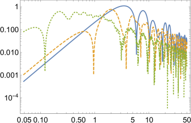
The analytic results for the x~~𝑥\tilde{x}-integral terms are given in Appendix B.3. Comparing (4.5) and (4.5), we see that they are clearly different and the gauge dependence of the scalar-induced GWs are persistent during RD. In Figure 4 we show the kernels in the both gauges.

Refer to caption
Refer to caption
Figure 4: The kernels for the scalar-scalar induced GWs during RD in the (left) zero-shear gauge (4.5) and (right) comoving gauge (4.5) as a function of kη𝑘𝜂k\eta. Since the kernels are also dependent on q𝑞q, we set (solid lines) q/k=0.05𝑞𝑘0.05q/k=0.05, (dashed lines) q/k=2𝑞𝑘2q/k=2 and (dotted lines) q/k=20𝑞𝑘20q/k=20.

4.6 Scalar-tensor induced GWs during RD

Next we consider the scalar-tensor induced GWs during RD. Again, we work first in the zero-shear gauge for the scalar perturbations. From the linear solutions during RD, the time derivatives of φχsubscript𝜑𝜒\varphi_{\chi} and hλsubscript𝜆h_{\lambda} are

φ˙χ(𝒒)subscript˙𝜑𝜒𝒒\displaystyle\dot{\varphi}_{\chi}({\bm{q}}) =2Hj2(qη3),absent2𝐻subscript𝑗2𝑞𝜂3\displaystyle=-2H{\cal R}j_{2}\bigg{(}\frac{q\eta}{\sqrt{3}}\bigg{)}\,, (77)
φ¨χ(𝒒)subscript¨𝜑𝜒𝒒\displaystyle\ddot{\varphi}_{\chi}({\bm{q}}) =2H2[5j2(qη3)qη3j1(qη3)],absent2superscript𝐻2delimited-[]5subscript𝑗2𝑞𝜂3𝑞𝜂3subscript𝑗1𝑞𝜂3\displaystyle=2H^{2}{\cal R}\bigg{[}5j_{2}\bigg{(}\frac{q\eta}{\sqrt{3}}\bigg{)}-\frac{q\eta}{\sqrt{3}}j_{1}\bigg{(}\frac{q\eta}{\sqrt{3}}\bigg{)}\bigg{]}\,, (78)
h˙λ(𝒒)subscript˙𝜆𝒒\displaystyle\dot{h}_{\lambda}({\bm{q}}) =Hqηh0λ(𝒒)j1(qη),absent𝐻𝑞𝜂superscriptsubscript0𝜆𝒒subscript𝑗1𝑞𝜂\displaystyle=-Hq\eta h_{0}^{\lambda}({\bm{q}})j_{1}(q\eta)\,, (79)
h¨λ(𝒒)subscript¨𝜆𝒒\displaystyle\ddot{h}_{\lambda}({\bm{q}}) =q2a2h0λ(𝒒)j2(qη).absentsuperscript𝑞2superscript𝑎2superscriptsubscript0𝜆𝒒subscript𝑗2𝑞𝜂\displaystyle=\frac{q^{2}}{a^{2}}h_{0}^{\lambda}({\bm{q}})j_{2}(q\eta)\,. (80)

Then with qη=q¯1x𝑞𝜂subscript¯𝑞1𝑥q\eta=\bar{q}_{1}x and |𝒌𝒒|η=q¯2x𝒌𝒒𝜂subscript¯𝑞2𝑥|{\bm{k}}-{\bm{q}}|\eta=\bar{q}_{2}x, we can write

sij(st)(𝒌)superscriptsubscript𝑠𝑖𝑗𝑠𝑡𝒌\displaystyle s_{ij}^{(st)}({\bm{k}}) =k2a2d3q(2π)3{2x2[2j2(q¯1x3)q¯1x3j1(q¯1x3)]j0(q¯2x)\displaystyle=\frac{k^{2}}{a^{2}}\int\frac{d^{3}q}{(2\pi)^{3}}\Bigg{\{}\frac{2}{x^{2}}\bigg{[}2j_{2}\bigg{(}\frac{\bar{q}_{1}x}{\sqrt{3}}\bigg{)}-\frac{\bar{q}_{1}x}{\sqrt{3}}j_{1}\bigg{(}\frac{\bar{q}_{1}x}{\sqrt{3}}\bigg{)}\bigg{]}j_{0}(\bar{q}_{2}x)
+2(1+|𝒌𝒒|2k2)j1(q¯1x/3)q¯1x/3j0(q¯2x)}(𝒒)hλ0(𝒌𝒒)eijλ(𝒌𝒒)\displaystyle\hskip 70.0001pt+2\bigg{(}1+\frac{|{\bm{k}}-{\bm{q}}|^{2}}{k^{2}}\bigg{)}\frac{j_{1}(\bar{q}_{1}x/\sqrt{3})}{\bar{q}_{1}x/\sqrt{3}}j_{0}(\bar{q}_{2}x)\Bigg{\}}{\cal R}({\bm{q}})h^{\lambda^{\prime}}_{0}({\bm{k}}-{\bm{q}})e_{ij}^{\lambda^{\prime}}({\bm{k}}-{\bm{q}})
+k2a2d3q(2π)3{2x2j0(q¯1x3)[2j2(q¯2x)q¯2xj1(q¯2x)]+2(1+q2k2)j0(q¯1x3)j1(q¯2x)q¯2x}(𝒌𝒒)h0λ(𝒒)eijλ(𝒒).superscript𝑘2superscript𝑎2superscript𝑑3𝑞superscript2𝜋32superscript𝑥2subscript𝑗0subscript¯𝑞1𝑥3delimited-[]2subscript𝑗2subscript¯𝑞2𝑥subscript¯𝑞2𝑥subscript𝑗1subscript¯𝑞2𝑥21superscript𝑞2superscript𝑘2subscript𝑗0subscript¯𝑞1𝑥3subscript𝑗1subscript¯𝑞2𝑥subscript¯𝑞2𝑥𝒌𝒒subscriptsuperscriptsuperscript𝜆0𝒒superscriptsubscript𝑒𝑖𝑗superscript𝜆𝒒\displaystyle\quad+\frac{k^{2}}{a^{2}}\int\frac{d^{3}q}{(2\pi)^{3}}\Bigg{\{}\frac{2}{x^{2}}j_{0}\bigg{(}\frac{\bar{q}_{1}x}{\sqrt{3}}\bigg{)}\bigg{[}2j_{2}(\bar{q}_{2}x)-\bar{q}_{2}xj_{1}(\bar{q}_{2}x)\bigg{]}+2\bigg{(}1+\frac{q^{2}}{k^{2}}\bigg{)}j_{0}\bigg{(}\frac{\bar{q}_{1}x}{\sqrt{3}}\bigg{)}\frac{j_{1}(\bar{q}_{2}x)}{\bar{q}_{2}x}\Bigg{\}}{\cal R}({\bm{k}}-{\bm{q}})h^{\lambda^{\prime}}_{0}({\bm{q}})e_{ij}^{\lambda^{\prime}}({\bm{q}})\,. (81)

We note that the first integral can be made identical to the second one upon defining 𝒌𝒒𝒑𝒌𝒒𝒑{\bm{k}}-{\bm{q}}\equiv{\bm{p}}, and then renaming the dummy integration variable 𝒑𝒑{\bm{p}} as 𝒒𝒒{\bm{q}}. Thus, the scalar-tensor source term in the zero-shear gauge is, after multiplying the polarization tensor eλij(𝒌)subscriptsuperscript𝑒𝑖𝑗𝜆𝒌e^{ij}_{\lambda}({\bm{k}}),

eλij(𝒌)sij(st)(𝒌)subscriptsuperscript𝑒𝑖𝑗𝜆𝒌superscriptsubscript𝑠𝑖𝑗𝑠𝑡𝒌\displaystyle e^{ij}_{\lambda}({\bm{k}})s_{ij}^{(st)}({\bm{k}}) =4k2a2d3q(2π)3[eλij(𝒌)eijλ(𝒒)](𝒌𝒒)h0λ(𝒒)absent4superscript𝑘2superscript𝑎2superscript𝑑3𝑞superscript2𝜋3delimited-[]subscriptsuperscript𝑒𝑖𝑗𝜆𝒌superscriptsubscript𝑒𝑖𝑗superscript𝜆𝒒𝒌𝒒subscriptsuperscriptsuperscript𝜆0𝒒\displaystyle=\frac{4k^{2}}{a^{2}}\int\frac{d^{3}q}{(2\pi)^{3}}\Big{[}e^{ij}_{\lambda}({\bm{k}})e_{ij}^{\lambda^{\prime}}({\bm{q}})\Big{]}{\cal R}({\bm{k}}-{\bm{q}})h^{\lambda^{\prime}}_{0}({\bm{q}})
×{1x2j0(q¯1x~3)[2j2(q¯2x)q¯2xj1(q¯2x)]+(1+q2k2)j0(q¯1x~3)j1(q¯2x)q¯2x}.absent1superscript𝑥2subscript𝑗0subscript¯𝑞1~𝑥3delimited-[]2subscript𝑗2subscript¯𝑞2𝑥subscript¯𝑞2𝑥subscript𝑗1subscript¯𝑞2𝑥1superscript𝑞2superscript𝑘2subscript𝑗0subscript¯𝑞1~𝑥3subscript𝑗1subscript¯𝑞2𝑥subscript¯𝑞2𝑥\displaystyle\hskip 30.00005pt\times\Bigg{\{}\frac{1}{x^{2}}j_{0}\bigg{(}\frac{\bar{q}_{1}\tilde{x}}{\sqrt{3}}\bigg{)}\bigg{[}2j_{2}(\bar{q}_{2}x)-\bar{q}_{2}xj_{1}(\bar{q}_{2}x)\bigg{]}+\bigg{(}1+\frac{q^{2}}{k^{2}}\bigg{)}j_{0}\bigg{(}\frac{\bar{q}_{1}\tilde{x}}{\sqrt{3}}\bigg{)}\frac{j_{1}(\bar{q}_{2}x)}{\bar{q}_{2}x}\Bigg{\}}\,. (82)

Then the solution is

hλ(η,𝒌)subscript𝜆𝜂𝒌\displaystyle h_{\lambda}(\eta,{\bm{k}}) =d3q(2π)3[eλij(𝒌)eijλ(𝒒)](𝒌𝒒)h0λ(𝒒)absentsuperscript𝑑3𝑞superscript2𝜋3delimited-[]subscriptsuperscript𝑒𝑖𝑗𝜆𝒌superscriptsubscript𝑒𝑖𝑗superscript𝜆𝒒𝒌𝒒subscriptsuperscriptsuperscript𝜆0𝒒\displaystyle=\int\frac{d^{3}q}{(2\pi)^{3}}\Big{[}e^{ij}_{\lambda}({\bm{k}})e_{ij}^{\lambda^{\prime}}({\bm{q}})\Big{]}{\cal R}({\bm{k}}-{\bm{q}})h^{\lambda^{\prime}}_{0}({\bm{q}})
×40x𝑑x~x~2{1x~2j0(q¯1x~3)[2j2(q¯2x~)q¯2x~j1(q¯2x~)]+(1+q¯12)j0(q¯1x~3)j1(q¯2x~)q¯2x~}[j0(x~)y0(x)j0(x)y0(x~)].absent4superscriptsubscript0𝑥differential-d~𝑥superscript~𝑥21superscript~𝑥2subscript𝑗0subscript¯𝑞1~𝑥3delimited-[]2subscript𝑗2subscript¯𝑞2~𝑥subscript¯𝑞2~𝑥subscript𝑗1subscript¯𝑞2~𝑥1superscriptsubscript¯𝑞12subscript𝑗0subscript¯𝑞1~𝑥3subscript𝑗1subscript¯𝑞2~𝑥subscript¯𝑞2~𝑥delimited-[]subscript𝑗0~𝑥subscript𝑦0𝑥subscript𝑗0𝑥subscript𝑦0~𝑥\displaystyle\quad\times 4\int_{0}^{x}d\tilde{x}\tilde{x}^{2}\Bigg{\{}\frac{1}{\tilde{x}^{2}}j_{0}\bigg{(}\frac{\bar{q}_{1}\tilde{x}}{\sqrt{3}}\bigg{)}\bigg{[}2j_{2}(\bar{q}_{2}\tilde{x})-\bar{q}_{2}\tilde{x}j_{1}(\bar{q}_{2}\tilde{x})\bigg{]}+\big{(}1+\bar{q}_{1}^{2}\big{)}j_{0}\bigg{(}\frac{\bar{q}_{1}\tilde{x}}{\sqrt{3}}\bigg{)}\frac{j_{1}(\bar{q}_{2}\tilde{x})}{\bar{q}_{2}\tilde{x}}\Bigg{\}}\Big{[}j_{0}(\tilde{x})y_{0}(x)-j_{0}(x)y_{0}(\tilde{x})\Big{]}\,. (83)

The x~~𝑥\tilde{x}-integral can be performed analytically and the individual integrations are given in Appendix B.4.

In the comoving gauge, similarly upon changing the dummy integration variable we can find the source term as

eλij(𝒌)sij(st)(𝒌)subscriptsuperscript𝑒𝑖𝑗𝜆𝒌superscriptsubscript𝑠𝑖𝑗𝑠𝑡𝒌\displaystyle e^{ij}_{\lambda}({\bm{k}})s_{ij}^{(st)}({\bm{k}}) =2k2a2d3q(2π)3[eλij(𝒌)eijλ(𝒒)](𝒌𝒒)h0λ(𝒒)[2(1q¯22)j0(q¯1x3)j0(q¯2x)+(1+q¯123+q¯22)q¯1x3j1(q¯1x3)j0(q¯2x)\displaystyle=\frac{2k^{2}}{a^{2}}\int\frac{d^{3}q}{(2\pi)^{3}}\Big{[}e^{ij}_{\lambda}({\bm{k}})e_{ij}^{\lambda^{\prime}}({\bm{q}})\Big{]}{\cal R}({\bm{k}}-{\bm{q}})h^{\lambda^{\prime}}_{0}({\bm{q}})\bigg{[}2(1-\bar{q}_{2}^{2})j_{0}\bigg{(}\frac{\bar{q}_{1}x}{\sqrt{3}}\bigg{)}j_{0}(\bar{q}_{2}x)+\bigg{(}-1+\frac{\bar{q}_{1}^{2}}{3}+\bar{q}_{2}^{2}\bigg{)}\frac{\bar{q}_{1}x}{\sqrt{3}}j_{1}\bigg{(}\frac{\bar{q}_{1}x}{\sqrt{3}}\bigg{)}j_{0}(\bar{q}_{2}x)
+2q¯123q¯2xj0(q¯1x3)j1(q¯2x)+2q¯1/3q¯2(1q¯12)j1(q¯1x3)j1(q¯2x)],\displaystyle\hskip 200.0003pt+2\frac{\bar{q}_{1}^{2}}{3}\bar{q}_{2}xj_{0}\bigg{(}\frac{\bar{q}_{1}x}{\sqrt{3}}\bigg{)}j_{1}(\bar{q}_{2}x)+2\frac{\bar{q}_{1}/\sqrt{3}}{\bar{q}_{2}}\big{(}1-\bar{q}_{1}^{2}\big{)}j_{1}\bigg{(}\frac{\bar{q}_{1}x}{\sqrt{3}}\bigg{)}j_{1}(\bar{q}_{2}x)\bigg{]}\,, (84)

so that the analytic integral solution for hλsubscript𝜆h_{\lambda} is

hλ(η,𝒌)subscript𝜆𝜂𝒌\displaystyle h_{\lambda}(\eta,{\bm{k}}) =d3q(2π)3[eλij(𝒌)eijλ(𝒒)](𝒌𝒒)h0λ(𝒒)absentsuperscript𝑑3𝑞superscript2𝜋3delimited-[]subscriptsuperscript𝑒𝑖𝑗𝜆𝒌superscriptsubscript𝑒𝑖𝑗superscript𝜆𝒒𝒌𝒒subscriptsuperscriptsuperscript𝜆0𝒒\displaystyle=\int\frac{d^{3}q}{(2\pi)^{3}}\Big{[}e^{ij}_{\lambda}({\bm{k}})e_{ij}^{\lambda^{\prime}}({\bm{q}})\Big{]}{\cal R}({\bm{k}}-{\bm{q}})h^{\lambda^{\prime}}_{0}({\bm{q}})
×20xdx~x~2[2(1q¯22)j0(q¯1x3)j0(q¯2x)+(1+q¯123+q¯22)q¯1x3j1(q¯1x3)j0(q¯2x)\displaystyle\quad\times 2\int_{0}^{x}d\tilde{x}\tilde{x}^{2}\bigg{[}2(1-\bar{q}_{2}^{2})j_{0}\bigg{(}\frac{\bar{q}_{1}x}{\sqrt{3}}\bigg{)}j_{0}(\bar{q}_{2}x)+\bigg{(}-1+\frac{\bar{q}_{1}^{2}}{3}+\bar{q}_{2}^{2}\bigg{)}\frac{\bar{q}_{1}x}{\sqrt{3}}j_{1}\bigg{(}\frac{\bar{q}_{1}x}{\sqrt{3}}\bigg{)}j_{0}(\bar{q}_{2}x)
+2q¯123q¯2xj0(q¯1x3)j1(q¯2x)+2q¯1/3q¯2(1q¯12)j1(q¯1x3)j1(q¯2x)][j0(x~)y0(x)j0(x)y0(x~)].\displaystyle\hskip 70.0001pt+2\frac{\bar{q}_{1}^{2}}{3}\bar{q}_{2}xj_{0}\bigg{(}\frac{\bar{q}_{1}x}{\sqrt{3}}\bigg{)}j_{1}(\bar{q}_{2}x)+2\frac{\bar{q}_{1}/\sqrt{3}}{\bar{q}_{2}}\big{(}1-\bar{q}_{1}^{2}\big{)}j_{1}\bigg{(}\frac{\bar{q}_{1}x}{\sqrt{3}}\bigg{)}j_{1}(\bar{q}_{2}x)\bigg{]}\Big{[}j_{0}(\tilde{x})y_{0}(x)-j_{0}(x)y_{0}(\tilde{x})\Big{]}\,. (85)

The details of each integration are given in Appendix B.4. In Figure 5, we show both kernels, (4.6) and (4.6).
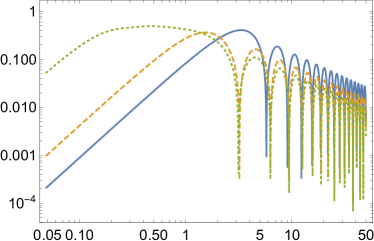
Refer to caption
Refer to caption
Figure 5: The kernels for the scalar-tensor induced GWs during RD in the (left) zero-shear gauge and (right) comoving gauge as a function of kη𝑘𝜂k\eta. Since the kernel is also dependent on the angle between 𝒌𝒌{\bm{k}} and 𝒒𝒒{\bm{q}}, for simplicity we set in such a way that for both (solid lines) q/k=0.05𝑞𝑘0.05q/k=0.05 and (dotted lines) q/k=20𝑞𝑘20q/k=20 they are aligned perpendicular, i.e. cos(𝒌^𝒒^)=0^𝒌^𝒒0\cos\big{(}\hat{\bm{k}}\cdot\hat{\bm{q}}\big{)}=0, while for (dashed lines) q/k=2𝑞𝑘2q/k=2 the angle between them is 2π/32𝜋32\pi/3, cos(𝒌^𝒒^)=1/2^𝒌^𝒒12\cos\big{(}\hat{\bm{k}}\cdot\hat{\bm{q}}\big{)}=-1/2.

4.7 Tensor-tensor induced GWs during RD

Next we consider the tensor-tensor induced GWs during RD. Working in a similar manner to MD, multiplying the polarization tensor eλij(𝒌)subscriptsuperscript𝑒𝑖𝑗𝜆𝒌e^{ij}_{\lambda}({\bm{k}}) gives

eλij(𝒌)sij(tt)(𝒌)subscriptsuperscript𝑒𝑖𝑗𝜆𝒌superscriptsubscript𝑠𝑖𝑗𝑡𝑡𝒌\displaystyle e^{ij}_{\lambda}({\bm{k}})s_{ij}^{(tt)}({\bm{k}}) =1a2d3q1d3q2(2π)3δ(3)(𝒌𝒒12){h0λ1(𝒒1)h0λ2(𝒒2)eλij(𝒌)q1q2ei1kλ1ejk2λ2𝒞~λ(𝒒1,𝒒2)j1(q1η)j1(q2η)\displaystyle=\frac{1}{a^{2}}\int\frac{d^{3}q_{1}d^{3}q_{2}}{(2\pi)^{3}}\delta^{(3)}({\bm{k}}-{\bm{q}}_{12})\bigg{\{}\underbrace{h_{0}^{\lambda_{1}}({\bm{q}}_{1})h_{0}^{\lambda_{2}}({\bm{q}}_{2})e^{ij}_{\lambda}({\bm{k}})q_{1}q_{2}e_{i1}^{k\lambda_{1}}e_{jk2}^{\lambda_{2}}}_{\equiv\widetilde{{\cal C}}_{\lambda}({\bm{q}}_{1},{\bm{q}}_{2})}j_{1}(q_{1}\eta)j_{1}(q_{2}\eta)
+h0λ1(𝒒1)h0λ2(𝒒2)eλij(𝒌)[eλ11kl(q2jq2keil2λ2q2iq2kejl2λ2+q2kq2leij2λ2)\displaystyle\hskip 100.00015pt+h_{0}^{\lambda_{1}}({\bm{q}}_{1})h_{0}^{\lambda_{2}}({\bm{q}}_{2})e^{ij}_{\lambda}({\bm{k}})\bigg{[}e^{kl}_{\lambda_{1}1}\big{(}-q_{2j}q_{2k}e^{\lambda_{2}}_{il2}-q_{2i}q_{2k}e_{jl2}^{\lambda_{2}}+q_{2k}q_{2l}e^{\lambda_{2}}_{ij2}\big{)}
+12q1iq1jeλ1kl1ekl2λ2+(𝒒1𝒒2)ei1kλ1ejk2λ2q1lq2kei1kλ1ejl2λ2]𝒟~λ(𝒒1,𝒒2)j0(q1η)j0(q2η)}\displaystyle\hskip 110.00017pt\underbrace{\hskip 80.00012pt+\frac{1}{2}q_{1i}q_{1j}e_{\lambda_{1}}^{kl1}e_{kl2}^{\lambda_{2}}+({\bm{q}}_{1}\cdot{\bm{q}}_{2})e_{i1}^{k\lambda_{1}}e_{jk2}^{\lambda_{2}}-q_{1}^{l}q_{2k}e_{i1}^{k\lambda_{1}}e_{jl2}^{\lambda_{2}}\bigg{]}}_{\equiv\widetilde{{\cal D}}_{\lambda}({\bm{q}}_{1},{\bm{q}}_{2})}j_{0}(q_{1}\eta)j_{0}(q_{2}\eta)\bigg{\}}
+(𝒒1𝒒2).\displaystyle\quad+({\bm{q}}_{1}\leftrightarrow{\bm{q}}_{2})\,. (86)

Thus, with x=kη𝑥𝑘𝜂x=k\eta, q¯1q1/ksubscript¯𝑞1subscript𝑞1𝑘\bar{q}_{1}\equiv q_{1}/k and q¯2q2/ksubscript¯𝑞2subscript𝑞2𝑘\bar{q}_{2}\equiv q_{2}/k,

hλ(η,𝒌)subscript𝜆𝜂𝒌\displaystyle h_{\lambda}(\eta,{\bm{k}}) =d3q1d3q2(2π)3δ(3)(𝒌𝒒12)1k2{[𝒞~λ(𝒒1,𝒒2)+(𝒒1𝒒2)]0xdx~x~2j1(q¯1x~)j1(q¯2x~)[j0(x~)y0(x)j0(x)y0(x~)]\displaystyle=\int\frac{d^{3}q_{1}d^{3}q_{2}}{(2\pi)^{3}}\delta^{(3)}({\bm{k}}-{\bm{q}}_{12})\frac{1}{k^{2}}\bigg{\{}\Big{[}\widetilde{{\cal C}}_{\lambda}({\bm{q}}_{1},{\bm{q}}_{2})+({\bm{q}}_{1}\leftrightarrow{\bm{q}}_{2})\Big{]}\int_{0}^{x}d\tilde{x}\tilde{x}^{2}j_{1}(\bar{q}_{1}\tilde{x})j_{1}(\bar{q}_{2}\tilde{x})\Big{[}j_{0}(\tilde{x})y_{0}(x)-j_{0}(x)y_{0}(\tilde{x})\Big{]}
+[𝒟~λ(𝒒1,𝒒2)+(𝒒1𝒒2)]0xdx~x~2j0(q¯1x~)j0(q¯2x~)[j0(x~)y0(x)j0(x)y0(x~)]}.\displaystyle\hskip 135.0002pt+\Big{[}\widetilde{{\cal D}}_{\lambda}({\bm{q}}_{1},{\bm{q}}_{2})+({\bm{q}}_{1}\leftrightarrow{\bm{q}}_{2})\Big{]}\int_{0}^{x}d\tilde{x}\tilde{x}^{2}j_{0}(\bar{q}_{1}\tilde{x})j_{0}(\bar{q}_{2}\tilde{x})\Big{[}j_{0}(\tilde{x})y_{0}(x)-j_{0}(x)y_{0}(\tilde{x})\Big{]}\bigg{\}}\,. (87)

The x~~𝑥\tilde{x}-integrals can be performed analytically and finally we can write

hλ(𝒌,η)subscript𝜆𝒌𝜂\displaystyle h_{\lambda}({\bm{k}},\eta) =d3q(2π)3h0λ1(𝒒)h0λ2(𝒌𝒒){eλij(𝒌)eikλ1(𝒒)ejkλ2(𝒌𝒒)FRD(𝒌,𝒒,η)\displaystyle=\int\frac{d^{3}q}{(2\pi)^{3}}h_{0}^{\lambda_{1}}({\bm{q}})h_{0}^{\lambda_{2}}({\bm{k}}-{\bm{q}})\Bigg{\{}e_{\lambda}^{ij}({\bm{k}})e_{i}^{k\lambda_{1}}({\bm{q}})e_{jk}^{\lambda_{2}}({\bm{k}}-{\bm{q}}){F}_{\text{RD}}({\bm{k}},{\bm{q}},\eta)
+1k2(eλij(𝒌)eλ1kl(𝒒)(qjkkeilλ2(𝒌𝒒)+qikkejlλ2(𝒌𝒒)+kkkleijλ2(𝒌𝒒))\displaystyle\hskip 15.00002pt+\frac{1}{k^{2}}\bigg{(}e_{\lambda}^{ij}({\bm{k}})e^{kl}_{\lambda_{1}}({\bm{q}})\Big{(}q_{j}k_{k}e_{il}^{\lambda_{2}}({\bm{k}}-{\bm{q}})+q_{i}k_{k}e_{jl}^{\lambda_{2}}({\bm{k}}-{\bm{q}})+k_{k}k_{l}e_{ij}^{\lambda_{2}}({\bm{k}}-{\bm{q}})\Big{)}
+eλij(𝒌)[12qiqjeλ1kl(𝒒)eklλ2(𝒌𝒒)+𝒒(𝒌𝒒)eikλ1(𝒒)ejkλ2(𝒌𝒒)qlkkeikλ1(𝒒)ejlλ2(𝒌𝒒)])GRD(𝒌,𝒒,η)},\displaystyle\hskip 20.00003pt+e_{\lambda}^{ij}({\bm{k}})\bigg{[}\frac{1}{2}q_{i}q_{j}e^{kl}_{\lambda_{1}}({\bm{q}})e_{kl}^{\lambda_{2}}({\bm{k}}-{\bm{q}})+{\bm{q}}\cdot({\bm{k}}-{\bm{q}})e_{i}^{k\lambda_{1}}({\bm{q}})e_{jk}^{\lambda_{2}}({\bm{k}}-{\bm{q}})-q^{l}k_{k}e_{i}^{k\lambda_{1}}({\bm{q}})e_{jl}^{\lambda_{2}}({\bm{k}}-{\bm{q}})\bigg{]}\bigg{)}{G}_{\text{RD}}({\bm{k}},{\bm{q}},\eta)\Bigg{\}}\,, (88)

where the kernels FRDsubscript𝐹RDF_{\text{RD}} and GRDsubscript𝐺RDG_{\text{RD}} are given respectively by (B.5) and (B.5). In Figure 6 we show FRDsubscript𝐹RDF_{\text{RD}} and GRDsubscript𝐺RDG_{\text{RD}}.

Refer to caption
Refer to caption
Figure 6: The kernels (left) FRDsubscript𝐹RDF_{\text{RD}} and (right) GRDsubscript𝐺RDG_{\text{RD}} as a function of kη𝑘𝜂k\eta. Since they are also dependent on the angle between 𝒌𝒌{\bm{k}} and 𝒒𝒒{\bm{q}}, for simplicity we set in such a way that for both (solid lines) q/k=0.05𝑞𝑘0.05q/k=0.05 and (dotted lines) q/k=20𝑞𝑘20q/k=20 they are aligned perpendicular, i.e. cos(𝒌^𝒒^)=0^𝒌^𝒒0\cos\big{(}\hat{\bm{k}}\cdot\hat{\bm{q}}\big{)}=0, while for (dashed lines) q/k=2𝑞𝑘2q/k=2 the angle between them is 2π/32𝜋32\pi/3, cos(𝒌^𝒒^)=1/2^𝒌^𝒒12\cos\big{(}\hat{\bm{k}}\cdot\hat{\bm{q}}\big{)}=-1/2 in both panels.

5 Conclusions

In this article, we have presented the equation of motion for the tensor perturbations up to second order in perturbations, including all possible quadratic combinations of different types of cosmological perturbations. These terms serve as sources to generate second-order GWs. Given that the universe is filled with a perfect fluid matter with vanishing anisotropic stress, only linear scalar and tensor perturbations contribute to the source terms. And we have found the analytic integral solutions for the second-order GWs during both MD and RD induced by the scalar-scalar, scalar-tensor and tensor-tensor sources. The transition between MD and RD can be considered by separating the time integral of (4.1). That is, for the transition from the epoch A𝐴A to the epoch B𝐵B at η=η𝜂subscript𝜂\eta=\eta_{\star}, we may write (Kohri, & Terada, 2018)

hλ(η,𝒌)=1a{0η𝑑η~a3(η)a3(η)[a3(η~)eλij(𝒌)sijA(𝒌)]GAB(η,η~)+ηη𝑑η~[a3(η~)eλij(𝒌)sijAB(𝒌)]GB(η,η~)},subscript𝜆𝜂𝒌1𝑎superscriptsubscript0subscript𝜂differential-d~𝜂superscript𝑎3𝜂superscript𝑎3subscript𝜂delimited-[]superscript𝑎3~𝜂subscriptsuperscript𝑒𝑖𝑗𝜆𝒌subscriptsuperscript𝑠𝐴𝑖𝑗𝒌subscript𝐺𝐴𝐵𝜂~𝜂superscriptsubscriptsubscript𝜂𝜂differential-d~𝜂delimited-[]superscript𝑎3~𝜂subscriptsuperscript𝑒𝑖𝑗𝜆𝒌subscriptsuperscript𝑠𝐴𝐵𝑖𝑗𝒌subscript𝐺𝐵𝜂~𝜂h_{\lambda}(\eta,{\bm{k}})=\frac{1}{a}\Bigg{\{}\int_{0}^{\eta_{\star}}d\tilde{\eta}\,\frac{a^{3}(\eta)}{a^{3}(\eta_{\star})}\Big{[}a^{3}(\tilde{\eta})e^{ij}_{\lambda}(\bm{k})s^{A}_{ij}(\bm{k})\Big{]}G_{A\to B}(\eta,\tilde{\eta})+\int_{\eta_{\star}}^{\eta}d\tilde{\eta}\,\Big{[}a^{3}(\tilde{\eta})e^{ij}_{\lambda}(\bm{k})s^{A\to B}_{ij}(\bm{k})\Big{]}G_{B}(\eta,\tilde{\eta})\Bigg{\}}\,, (89)

where the first term represents the change of the propagation of the GWs produced during A𝐴A through B𝐵B, and the second term denotes the modification of the source. These terms can be found by matching, for the first term, the solutions and, for the second term, the kernels. However given the complicated source terms, it is a formidable task to compute the effects of the transition analytically, so we do not proceed any further but are satisfied with the above schematic form, which can in principle be further manipulated.

Since the primary tensor perturbations are persistent irrespective of the sources, it is interesting to discuss if the tensor-induced GWs could ever be observationally significant. To address this question quantitatively, it is necessary to study further the relation between the tensor-induced GWs and the primary GWs. For example, if the primary GWs exhibit a sharp peak around at a certain scale k𝑘k, the corresponding tensor-induced GWs are likely to be more prominent than the primary ones over a broader range of the wavenumber other than the peak. In this regards, the tensor-induced GWs may serve as a useful tool to probe the shape of the primary GWs and the relevant underlying physics. It is also interesting to consider how to test the origin of the induced GWs. We may consider, for example, the scalar-scalar-tensor bispectrum, hdelimited-⟨⟩\langle{\cal R}{\cal R}h\rangle. If the tensor mode is scalar-induced, i.e. hsimilar-toh\sim{\cal R}{\cal R}, the bispectrum is directly related to the local-type scalar bispectrum. If, on the other hand, the tensor mode is induced by the primary GWs, hdelimited-⟨⟩\langle{\cal R}{\cal R}h\rangle is proportional to the product of the scalar and tensor power spectra. Higher-order correlation functions may thus be able to serve as a possible tool to test the origin of the induced tensor perturbations.

As the kernels that involve rapid oscillations are analytically specified, the solutions given in this article should be useful for analytic and/or numerical studies of the second-order induced GWs.

Acknowledgements

I thank Jai-chan Hwang, Donghui Jeong, Kazunori Kohri, Sachiko Kuroyanagi, Takahiro Terada and Jaiyul Yoo for helpful comments and discussions. I also thank the anonymous referee for her/his constructive feedback that improved the content of this article. This work is supported in part by the Basic Science Research Program (2016R1D1A1B03930408) and Mid-career Research Program (2019R1A2C2085023) through the National Research Foundation of Korea Research Grants. I also acknowledge the Korea-Japan Basic Scientific Cooperation Program supported by the National Research Foundation of Korea and the Japan Society for the Promotion of Science (2018K2A9A2A08000127 and 2020K2A9A2A08000097) and the Ewha Womans University Research Grant of 2020 (1-2020-1630-001-1). I am grateful to the Asia Pacific Center for Theoretical Physics for Focus Research Program “The origin and evolution of the Universe” where parts of this work were presented and discussed.

Appendix A Traceless evolution equation for the spatial metric

The traceless evolution equation for the spatial metric is written compactly using the Arnowitt-Deser-Misner formulation (Arnowitt et al., 2008). With the metric

ds2=N2(dx0)2+γij(Nidx0+dxi)(Njdx0+dxj),𝑑superscript𝑠2superscript𝑁2superscript𝑑superscript𝑥02subscript𝛾𝑖𝑗superscript𝑁𝑖𝑑superscript𝑥0𝑑superscript𝑥𝑖superscript𝑁𝑗𝑑superscript𝑥0𝑑superscript𝑥𝑗ds^{2}=-N^{2}(dx^{0})^{2}+\gamma_{ij}(N^{i}dx^{0}+dx^{i})(N^{j}dx^{0}+dx^{j})\,, (A.1)

where N𝑁N, Nisuperscript𝑁𝑖N^{i} and γijsubscript𝛾𝑖𝑗\gamma_{ij} denote respectively the lapse function, shift vector and spatial metric, the dynamics of the space-time is described by the spatial metric γijsubscript𝛾𝑖𝑗\gamma_{ij} through the curvature variables of the spatial hypersurfaces. Along with the matter contents residing in the space-time, the geometric equations for the curvature variables constitute a complete set of the equations of motion. The extrinsic curvature Kijsubscript𝐾𝑖𝑗K_{ij} is introduced as

Kij12N(Ni|j+Nj|iγij,0),subscript𝐾𝑖𝑗12𝑁subscript𝑁conditional𝑖𝑗subscript𝑁conditional𝑗𝑖subscript𝛾𝑖𝑗0K_{ij}\equiv\frac{1}{2N}\big{(}N_{i|j}+N_{j|i}-\gamma_{ij,0}\big{)}\,, (A.2)

where a vertical bar denotes a covariant derivative with respect to γijsubscript𝛾𝑖𝑗\gamma_{ij}. The evolution equation for the traceless part K¯ij=KijγijK/3subscript¯𝐾𝑖𝑗subscript𝐾𝑖𝑗subscript𝛾𝑖𝑗𝐾3\overline{K}_{ij}=K_{ij}-\gamma_{ij}K/3 with KKiiK\equiv K^{i}{}_{i} is

K¯ij,0NK¯iNkj|kN+K¯kNij|kNK¯iNkk|jN=KK¯ij1N(N|i|jδij3N|k)|k+R¯ij8πGT¯i,j\frac{\overline{K}^{i}{}_{j,0}}{N}-\frac{\overline{K}^{i}{}_{j|k}N^{k}}{N}+\frac{\overline{K}^{k}{}_{j}N^{i}{}_{|k}}{N}-\frac{\overline{K}^{i}{}_{k}N^{k}{}_{|j}}{N}=K\overline{K}^{i}{}_{j}-\frac{1}{N}\left(N^{|i}{}_{|j}-\frac{\delta^{i}{}_{j}}{3}N^{|k}{}_{|k}\right)+\overline{R}^{i}{}_{j}-8\pi G\overline{T}^{i}{}_{j}\,, (A.3)

where R¯ijsubscript¯𝑅𝑖𝑗\overline{R}_{ij} is the traceless part of the intrinsic curvature tensor Rijsubscript𝑅𝑖𝑗R_{ij} constructed from γijsubscript𝛾𝑖𝑗\gamma_{ij}. This is fully non-linear, geometric equation. To incorporate cosmological perturbations, we expand it perturbatively up to desired accuracy (Noh, & Hwang, 2004; Hwang, & Noh, 2007), or write the exact non-linear equation for cosmological perturbations (Gong et al., 2017). Using (1) and expanding up to second order in perturbations, this equation is written as

h¨i+j3Hh˙ijΔa2hi+j1a2{[a2ddt(χ(i,j)a2)+3Hχ(i],j)δij3[a2ddt(χk,ka2)+3Hχk],k}\displaystyle\ddot{h}^{i}{}_{j}+3H\dot{h}^{i}{}_{j}-\frac{\Delta}{a^{2}}h^{i}{}_{j}+\frac{1}{a^{2}}\left\{\left[a^{2}\frac{d}{dt}\left(\frac{\chi^{(i}{}_{,j)}}{a^{2}}\right)+3H\chi^{(i}{}_{,j)}\right]-\frac{\delta^{i}{}_{j}}{3}\left[a^{2}\frac{d}{dt}\left(\frac{\chi^{k}{}_{,k}}{a^{2}}\right)+3H\chi^{k}{}_{,k}\right]\right\}
1a2(ijδij3Δ)(α+φ)8πG(Πijδij3Πk)k\displaystyle-\frac{1}{a^{2}}\bigg{(}\partial^{i}\partial_{j}-\frac{\delta^{i}{}_{j}}{3}\Delta\bigg{)}(\alpha+\varphi)-8\pi G\bigg{(}\Pi^{i}{}_{j}-\frac{\delta^{i}{}_{j}}{3}\Pi^{k}{}_{k}\bigg{)}
=\displaystyle= ddt[(h˙i+jχ(i,j)a2)α+2(φδik+hik)(h˙jk+χ(k,j)a2)+2hikφ˙δjk+χka2(φ,iδjk+φ,jδikφ,kδi+jhi+k,jhjk,ihi)j,k]\displaystyle\frac{d}{dt}\left[\left(\dot{h}^{i}{}_{j}+\frac{\chi^{(i}{}_{,j)}}{a^{2}}\right)\alpha+2\big{(}\varphi\delta^{ik}+h^{ik}\big{)}\bigg{(}\dot{h}_{jk}+\frac{\chi_{(k,j)}}{a^{2}}\bigg{)}+2h^{ik}\dot{\varphi}\delta_{jk}+\frac{\chi^{k}}{a^{2}}\Big{(}\varphi^{,i}\delta_{jk}+\varphi_{,j}\delta^{i}{}_{k}-\varphi_{,k}\delta^{i}{}_{j}+h^{i}{}_{k,j}+h_{jk}{}^{,i}-h^{i}{}_{j,k}\Big{)}\right]
+3H[(h˙ji+χ(i,j)a2)α+2(φδik+hik)(h˙jk+χ(k,j)a2)+2hikφ˙δjk+χka2(φ,iδjk+φ,jδikφ,kδi+jhi+k,jhjk,ihi)j,k]\displaystyle+3H\left[\left(\dot{h}^{i}_{j}+\frac{\chi^{(i}{}_{,j)}}{a^{2}}\right)\alpha+2\big{(}\varphi\delta^{ik}+h^{ik}\big{)}\bigg{(}\dot{h}_{jk}+\frac{\chi_{(k,j)}}{a^{2}}\bigg{)}+2h^{ik}\dot{\varphi}\delta_{jk}+\frac{\chi^{k}}{a^{2}}\Big{(}\varphi^{,i}\delta_{jk}+\varphi_{,j}\delta^{i}{}_{k}-\varphi_{,k}\delta^{i}{}_{j}+h^{i}{}_{k,j}+h_{jk}{}^{,i}-h^{i}{}_{j,k}\Big{)}\right]
+αddt(h˙i+jχ(i,j)a2)χka2(h˙i+j,k1a2χ(i),j)k+κ(h˙i+j1a2χ(i),j)\displaystyle+\alpha\frac{d}{dt}\left(\dot{h}^{i}{}_{j}+\frac{\chi^{(i}{}_{,j)}}{a^{2}}\right)-\frac{\chi^{k}}{a^{2}}\bigg{(}\dot{h}^{i}{}_{j,k}+\frac{1}{a^{2}}\chi^{(i}{}_{,j)k}\bigg{)}+\kappa\bigg{(}\dot{h}^{i}{}_{j}+\frac{1}{a^{2}}\chi^{(i}{}_{,j)}\bigg{)}
δij3{ddt[χk,ka2α+2(φδkl+hkl)χ(k,l)a2+2hklh˙kl1a2χkφ,k]+3H[χk,ka2α+2(φδkl+hkl)χ(k,l)a2+2hklh˙kl1a2χkφ,k]\displaystyle-\frac{\delta^{i}{}_{j}}{3}\Bigg{\{}\frac{d}{dt}\left[\frac{\chi^{k}{}_{,k}}{a^{2}}\alpha+2\big{(}\varphi\delta^{kl}+h^{kl}\big{)}\frac{\chi_{(k,l)}}{a^{2}}+2h^{kl}\dot{h}_{kl}-\frac{1}{a^{2}}\chi^{k}\varphi_{,k}\right]+3H\left[\frac{\chi^{k}{}_{,k}}{a^{2}}\alpha+2\big{(}\varphi\delta^{kl}+h^{kl}\big{)}\frac{\chi_{(k,l)}}{a^{2}}+2h^{kl}\dot{h}_{kl}-\frac{1}{a^{2}}\chi^{k}\varphi_{,k}\right]
+αddt(χk,ka2)χka21a2χl+,lkκχk,ka2}+1a2χi,k(h˙k+j1a2χ(k),j1a2χk,j(h˙i+k1a2χ(i),k\displaystyle\hskip 30.00005pt+\alpha\frac{d}{dt}\left(\frac{\chi^{k}{}_{,k}}{a^{2}}\right)-\frac{\chi^{k}}{a^{2}}\frac{1}{a^{2}}\chi^{l}{}_{,lk}+\kappa\frac{\chi^{k}{}_{,k}}{a^{2}}\Bigg{\}}+\frac{1}{a^{2}}\chi^{i}{}_{,k}\bigg{(}\dot{h}^{k}{}_{j}+\frac{1}{a^{2}}\chi^{(k}{}_{,j}\bigg{)}-\frac{1}{a^{2}}\chi^{k}{}_{,j}\bigg{(}\dot{h}^{i}{}_{k}+\frac{1}{a^{2}}\chi^{(i}{}_{,k}\bigg{)}
+1a2{αα,i+,j12(α2+1a2χlχl),i,j2(φδik+hik)α,jk(φ,jδi+khi+k,jφ,iδjk+hjk,iφ,kδijhi)j,kα,k}\displaystyle+\frac{1}{a^{2}}\left\{-\alpha\alpha^{,i}{}_{,j}+\frac{1}{2}\bigg{(}-\alpha^{2}+\frac{1}{a^{2}}\chi^{l}\chi_{l}\bigg{)}^{,i}{}_{,j}-2\big{(}\varphi\delta^{ik}+h^{ik}\big{)}\alpha_{,jk}-\Big{(}\varphi_{,j}\delta^{i}{}_{k}+h^{i}{}_{k,j}+\varphi^{,i}\delta_{jk}+h_{jk}{}^{,i}-\varphi_{,k}\delta^{i}{}_{j}-h^{i}{}_{j,k}\Big{)}\alpha^{,k}\right\}
δij3{1a2[αΔα+12Δ(α2+1a2χkχk)2(φδkl+hkl)α,kl+φ,kα,k]}\displaystyle-\frac{\delta^{i}{}_{j}}{3}\left\{\frac{1}{a^{2}}\bigg{[}-\alpha\Delta\alpha+\frac{1}{2}\Delta\bigg{(}-\alpha^{2}+\frac{1}{a^{2}}\chi^{k}\chi_{k}\bigg{)}-2\big{(}\varphi\delta^{kl}+h^{kl}\big{)}\alpha_{,kl}+\varphi^{,k}\alpha_{,k}\bigg{]}\right\}
+1a2[3φ,iφ,i4φφ,i,j4φΔhij2hiΔjφ+φ,khik+,jφ,khjk,i3φ,khi+j,k2φ,ikhjk\displaystyle+\frac{1}{a^{2}}\bigg{[}-3\varphi^{,i}\varphi_{,i}-4\varphi\varphi^{,i}{}_{,j}-4\varphi\Delta{h}^{i}{}_{j}-2h^{i}{}_{j}\Delta\varphi+\varphi_{,k}h^{ik}{}_{,j}+\varphi^{,k}h_{jk}{}^{,i}-3\varphi^{,k}h^{i}{}_{j,k}+2\varphi^{,ik}h_{jk}
2hikΔhkj2hklhkl,j,ihkl,ihkl,j2hik,lhjk,l+2hik,lhjl,k2hkl(hi+l,jkhjl,k,ihi)j,kl\displaystyle\qquad-2h^{ik}\Delta{h}_{kj}-2h^{kl}h_{kl,j}{}^{,i}-h^{kl,i}h_{kl,j}-2h^{ik,l}h_{jk,l}+2h^{ik,l}h_{jl,k}-2h^{kl}\Big{(}h^{i}{}_{l,jk}+h_{jl,k}{}^{,i}-h^{i}{}_{j,kl}\Big{)}
δij3(3φ,kφ,k4φΔφ+2φ,klh,kl4hklΔhkl3hkl,mhkl,m+2hkl,mhkm,l)]\displaystyle\qquad-\frac{\delta^{i}{}_{j}}{3}\Big{(}-3\varphi^{,k}\varphi_{,k}-4\varphi\Delta\varphi+2\varphi^{,kl}h_{,kl}-4h^{kl}\Delta{h}_{kl}-3h^{kl,m}h_{kl,m}+2h^{kl,m}h_{km,l}\Big{)}\bigg{]}
16πG[(φδik+hik)Πjkδij3(φδkl+hkl)Πkl]+8πG(ρ+p)(vivjδij3vkvk).\displaystyle-16\pi G\bigg{[}\Big{(}\varphi\delta^{ik}+h^{ik}\Big{)}\Pi_{jk}-\frac{\delta^{i}{}_{j}}{3}\big{(}\varphi\delta^{kl}+h^{kl}\big{)}\Pi_{kl}\bigg{]}+8\pi G(\rho+p)\bigg{(}v^{i}v_{j}-\frac{\delta^{i}{}_{j}}{3}v^{k}v_{k}\bigg{)}\,. (A.4)

Appendix B Integrals of Bessel functions

Here, a𝑎a, b𝑏b and c𝑐c denote arbitrary positive constants.

B.1 Integrals for scalar-scalar and scalar-tensor induced GWs during MD

For sij(ss)superscriptsubscript𝑠𝑖𝑗𝑠𝑠s_{ij}^{(ss)} during MD, we have for the zero-shear gauge the following integrals for the spherical Bessel functions:

0x𝑑x~x~3j1(x~)superscriptsubscript0𝑥differential-d~𝑥superscript~𝑥3subscript𝑗1~𝑥\displaystyle\int_{0}^{x}d\tilde{x}\tilde{x}^{3}j_{1}(\tilde{x}) =3x2j1(x)x3j0(x),absent3superscript𝑥2subscript𝑗1𝑥superscript𝑥3subscript𝑗0𝑥\displaystyle=3x^{2}j_{1}(x)-x^{3}j_{0}(x)\,, (B.1)
0x𝑑x~x~3y1(x~)superscriptsubscript0𝑥differential-d~𝑥superscript~𝑥3subscript𝑦1~𝑥\displaystyle\int_{0}^{x}d\tilde{x}\tilde{x}^{3}y_{1}(\tilde{x}) =3+3x2y1(x)x3y0(x),absent33superscript𝑥2subscript𝑦1𝑥superscript𝑥3subscript𝑦0𝑥\displaystyle=3+3x^{2}y_{1}(x)-x^{3}y_{0}(x)\,, (B.2)

along with the following identities of the spherical Bessel functions:

(1xddx)m[xn+1fn(x)]superscript1𝑥𝑑𝑑𝑥𝑚delimited-[]superscript𝑥𝑛1subscript𝑓𝑛𝑥\displaystyle\bigg{(}\frac{1}{x}\frac{d}{dx}\bigg{)}^{m}\Big{[}x^{n+1}f_{n}(x)\Big{]} =xnm+1fnm(x),absentsuperscript𝑥𝑛𝑚1subscript𝑓𝑛𝑚𝑥\displaystyle=x^{n-m+1}f_{n-m}(x)\,, (B.3)
fn1+fn+1subscript𝑓𝑛1subscript𝑓𝑛1\displaystyle f_{n-1}+f_{n+1} =2n+1xfn.absent2𝑛1𝑥subscript𝑓𝑛\displaystyle=\frac{2n+1}{x}f_{n}\,. (B.4)

Also, we have the following integrals for the comoving gauge:

0x𝑑x~x~5j1(x~)superscriptsubscript0𝑥differential-d~𝑥superscript~𝑥5subscript𝑗1~𝑥\displaystyle\int_{0}^{x}d\tilde{x}\tilde{x}^{5}j_{1}(\tilde{x}) =5x2(x26)j1(x)x3(x210)j0(x),absent5superscript𝑥2superscript𝑥26subscript𝑗1𝑥superscript𝑥3superscript𝑥210subscript𝑗0𝑥\displaystyle=5x^{2}(x^{2}-6)j_{1}(x)-x^{3}(x^{2}-10)j_{0}(x)\,, (B.5)
0x𝑑x~x~5y1(x~)superscriptsubscript0𝑥differential-d~𝑥superscript~𝑥5subscript𝑦1~𝑥\displaystyle\int_{0}^{x}d\tilde{x}\tilde{x}^{5}y_{1}(\tilde{x}) =30+5x2(x26)y1(x)x3(x210)y0(x).absent305superscript𝑥2superscript𝑥26subscript𝑦1𝑥superscript𝑥3superscript𝑥210subscript𝑦0𝑥\displaystyle=-30+5x^{2}(x^{2}-6)y_{1}(x)-x^{3}(x^{2}-10)y_{0}(x)\,. (B.6)

For sij(st)superscriptsubscript𝑠𝑖𝑗𝑠𝑡s_{ij}^{(st)} during MD, for the zero-shear gauge,

0x𝑑x~x~2j1(ax~)j1(x~)superscriptsubscript0𝑥differential-d~𝑥superscript~𝑥2subscript𝑗1𝑎~𝑥subscript𝑗1~𝑥\displaystyle\int_{0}^{x}d\tilde{x}\tilde{x}^{2}j_{1}(a\tilde{x})j_{1}(\tilde{x}) =1a21[x2j1(ax)j0(x)ax2j0(ax)j1(x)],absent1superscript𝑎21delimited-[]superscript𝑥2subscript𝑗1𝑎𝑥subscript𝑗0𝑥𝑎superscript𝑥2subscript𝑗0𝑎𝑥subscript𝑗1𝑥\displaystyle=\frac{1}{a^{2}-1}\Big{[}x^{2}j_{1}(ax)j_{0}(x)-ax^{2}j_{0}(ax)j_{1}(x)\Big{]}\,, (B.7)
0x𝑑x~x~2j1(ax~)y1(x~)superscriptsubscript0𝑥differential-d~𝑥superscript~𝑥2subscript𝑗1𝑎~𝑥subscript𝑦1~𝑥\displaystyle\int_{0}^{x}d\tilde{x}\tilde{x}^{2}j_{1}(a\tilde{x})y_{1}(\tilde{x}) =1a21[a+x2j1(ax)y0(x)ax2j0(ax)y1(x)].absent1superscript𝑎21delimited-[]𝑎superscript𝑥2subscript𝑗1𝑎𝑥subscript𝑦0𝑥𝑎superscript𝑥2subscript𝑗0𝑎𝑥subscript𝑦1𝑥\displaystyle=\frac{1}{a^{2}-1}\Big{[}-a+x^{2}j_{1}(ax)y_{0}(x)-ax^{2}j_{0}(ax)y_{1}(x)\Big{]}\,. (B.8)

These give a rather simple result:

0x𝑑x~x~2j1(ax~)[j1(x~)y1(x)j1(x)y1(x~)]superscriptsubscript0𝑥differential-d~𝑥superscript~𝑥2subscript𝑗1𝑎~𝑥delimited-[]subscript𝑗1~𝑥subscript𝑦1𝑥subscript𝑗1𝑥subscript𝑦1~𝑥\displaystyle\int_{0}^{x}d\tilde{x}\tilde{x}^{2}j_{1}(a\tilde{x})\Big{[}j_{1}(\tilde{x})y_{1}(x)-j_{1}(x)y_{1}(\tilde{x})\Big{]} =1a21[aj1(x)j1(ax)].absent1superscript𝑎21delimited-[]𝑎subscript𝑗1𝑥subscript𝑗1𝑎𝑥\displaystyle=\frac{1}{a^{2}-1}\Big{[}aj_{1}(x)-j_{1}(ax)\Big{]}\,. (B.9)

For the comoving gauge, we have the following integrals:

0x𝑑x~x~3j0(ax~)j1(x~)superscriptsubscript0𝑥differential-d~𝑥superscript~𝑥3subscript𝑗0𝑎~𝑥subscript𝑗1~𝑥\displaystyle\int_{0}^{x}d\tilde{x}\tilde{x}^{3}j_{0}(a\tilde{x})j_{1}(\tilde{x}) =x2(a21)2{j0(x)[(a21)xj0(ax)2aj1(ax)]+j1(x)[(a23)j0(ax)+(a21)axj1(ax)]},absentsuperscript𝑥2superscriptsuperscript𝑎212subscript𝑗0𝑥delimited-[]superscript𝑎21𝑥subscript𝑗0𝑎𝑥2𝑎subscript𝑗1𝑎𝑥subscript𝑗1𝑥delimited-[]superscript𝑎23subscript𝑗0𝑎𝑥superscript𝑎21𝑎𝑥subscript𝑗1𝑎𝑥\displaystyle=\frac{x^{2}}{(a^{2}-1)^{2}}\Big{\{}j_{0}(x)\big{[}(a^{2}-1)xj_{0}(ax)-2aj_{1}(ax)\big{]}+j_{1}(x)\big{[}-(a^{2}-3)j_{0}(ax)+(a^{2}-1)axj_{1}(ax)\big{]}\Big{\}}\,, (B.10)
0x𝑑x~x~3j0(ax~)y1(x~)superscriptsubscript0𝑥differential-d~𝑥superscript~𝑥3subscript𝑗0𝑎~𝑥subscript𝑦1~𝑥\displaystyle\int_{0}^{x}d\tilde{x}\tilde{x}^{3}j_{0}(a\tilde{x})y_{1}(\tilde{x}) =1(a21)2{3a2+x2j0(ax)[(a21)xy0(x)(a23)y1(x)]\displaystyle=\frac{1}{(a^{2}-1)^{2}}\Big{\{}3-a^{2}+x^{2}j_{0}(ax)\big{[}(a^{2}-1)xy_{0}(x)-(a^{2}-3)y_{1}(x)\big{]}
+ax2j1(ax)[2y0(x)+(a21)xy1(x)]}.\displaystyle\hskip 60.00009pt+ax^{2}j_{1}(ax)\big{[}-2y_{0}(x)+(a^{2}-1)xy_{1}(x)\big{]}\Big{\}}\,. (B.11)

Again, we find a rather simple result from these integrals:

0x𝑑x~x~3j0(ax~)[j1(x~)y1(x)j1(x)y1(x~)]superscriptsubscript0𝑥differential-d~𝑥superscript~𝑥3subscript𝑗0𝑎~𝑥delimited-[]subscript𝑗1~𝑥subscript𝑦1𝑥subscript𝑗1𝑥subscript𝑦1~𝑥\displaystyle\int_{0}^{x}d\tilde{x}\tilde{x}^{3}j_{0}(a\tilde{x})\Big{[}j_{1}(\tilde{x})y_{1}(x)-j_{1}(x)y_{1}(\tilde{x})\Big{]} =1(a21)2[(a23)j1(x)+2aj1(ax)(a21)xj0(ax)].absent1superscriptsuperscript𝑎212delimited-[]superscript𝑎23subscript𝑗1𝑥2𝑎subscript𝑗1𝑎𝑥superscript𝑎21𝑥subscript𝑗0𝑎𝑥\displaystyle=\frac{1}{(a^{2}-1)^{2}}\Big{[}(a^{2}-3)j_{1}(x)+2aj_{1}(ax)-(a^{2}-1)xj_{0}(ax)\Big{]}\,. (B.12)

B.2 Integrals for tensor-tensor induced GWs during MD

They can be arranged as, for the first two integrals,

0x𝑑x~x~j2(ax~)j2(bx~)j1(cx~)superscriptsubscript0𝑥differential-d~𝑥~𝑥subscript𝑗2𝑎~𝑥subscript𝑗2𝑏~𝑥subscript𝑗1𝑐~𝑥\displaystyle\int_{0}^{x}d\tilde{x}\tilde{x}j_{2}(a\tilde{x})j_{2}(b\tilde{x})j_{1}(c\tilde{x})
=(a2+b2c2)(a2b2c2)x216ab2cj1(ax)j0(bx)j0(cx)(a2+b2c2)(a2b2+c2)x216a2bcj0(ax)j1(bx)j0(cx)absentsuperscript𝑎2superscript𝑏2superscript𝑐2superscript𝑎2superscript𝑏2superscript𝑐2superscript𝑥216𝑎superscript𝑏2𝑐subscript𝑗1𝑎𝑥subscript𝑗0𝑏𝑥subscript𝑗0𝑐𝑥superscript𝑎2superscript𝑏2superscript𝑐2superscript𝑎2superscript𝑏2superscript𝑐2superscript𝑥216superscript𝑎2𝑏𝑐subscript𝑗0𝑎𝑥subscript𝑗1𝑏𝑥subscript𝑗0𝑐𝑥\displaystyle=\frac{(a^{2}+b^{2}-c^{2})(a^{2}-b^{2}-c^{2})x^{2}}{16ab^{2}c}j_{1}(ax)j_{0}(bx)j_{0}(cx)-\frac{(a^{2}+b^{2}-c^{2})(a^{2}-b^{2}+c^{2})x^{2}}{16a^{2}bc}j_{0}(ax)j_{1}(bx)j_{0}(cx)
(a2+b2c2)2x216a2b2j0(ax)j0(bx)j1(cx)+x2aj1(ax)j0(bx)j1(cx)+x2bj0(ax)j1(bx)j1(cx)cx2abj1(ax)j1(bx)j0(cx)superscriptsuperscript𝑎2superscript𝑏2superscript𝑐22superscript𝑥216superscript𝑎2superscript𝑏2subscript𝑗0𝑎𝑥subscript𝑗0𝑏𝑥subscript𝑗1𝑐𝑥𝑥2𝑎subscript𝑗1𝑎𝑥subscript𝑗0𝑏𝑥subscript𝑗1𝑐𝑥𝑥2𝑏subscript𝑗0𝑎𝑥subscript𝑗1𝑏𝑥subscript𝑗1𝑐𝑥𝑐𝑥2𝑎𝑏subscript𝑗1𝑎𝑥subscript𝑗1𝑏𝑥subscript𝑗0𝑐𝑥\displaystyle\quad-\frac{(a^{2}+b^{2}-c^{2})^{2}x^{2}}{16a^{2}b^{2}}j_{0}(ax)j_{0}(bx)j_{1}(cx)+\frac{x}{2a}j_{1}(ax)j_{0}(bx)j_{1}(cx)+\frac{x}{2b}j_{0}(ax)j_{1}(bx)j_{1}(cx)-\frac{cx}{2ab}j_{1}(ax)j_{1}(bx)j_{0}(cx)
(a2+b2c2)x2+128abj1(ax)j1(bx)j1(cx)superscript𝑎2superscript𝑏2superscript𝑐2superscript𝑥2128𝑎𝑏subscript𝑗1𝑎𝑥subscript𝑗1𝑏𝑥subscript𝑗1𝑐𝑥\displaystyle\quad-\frac{(a^{2}+b^{2}-c^{2})x^{2}+12}{8ab}j_{1}(ax)j_{1}(bx)j_{1}(cx)
+(abc)(a+bc)(ab+c)(a+b+c)(a2+b2c2)64a3b3c2𝑎𝑏𝑐𝑎𝑏𝑐𝑎𝑏𝑐𝑎𝑏𝑐superscript𝑎2superscript𝑏2superscript𝑐264superscript𝑎3superscript𝑏3superscript𝑐2\displaystyle\quad+\frac{(a-b-c)(a+b-c)(a-b+c)(a+b+c)(a^{2}+b^{2}-c^{2})}{64a^{3}b^{3}c^{2}}
×{Si[(abc)x]Si[(a+bc)x]Si[(ab+c)x]+Si[(a+b+c)x]},absentSidelimited-[]𝑎𝑏𝑐𝑥Sidelimited-[]𝑎𝑏𝑐𝑥Sidelimited-[]𝑎𝑏𝑐𝑥Sidelimited-[]𝑎𝑏𝑐𝑥\displaystyle\qquad\times\Big{\{}{\rm Si}[(a-b-c)x]-{\rm Si}[(a+b-c)x]-{\rm Si}[(a-b+c)x]+{\rm Si}[(a+b+c)x]\Big{\}}\,, (B.13)
0x𝑑x~x~j2(ax~)j2(bx~)y1(cx~)superscriptsubscript0𝑥differential-d~𝑥~𝑥subscript𝑗2𝑎~𝑥subscript𝑗2𝑏~𝑥subscript𝑦1𝑐~𝑥\displaystyle\int_{0}^{x}d\tilde{x}\tilde{x}j_{2}(a\tilde{x})j_{2}(b\tilde{x})y_{1}(c\tilde{x})
=(a2+b2c2)(a2b2c2)x216ab2cj1(ax)j0(bx)y0(cx)(a2+b2c2)(a2b2+c2)x216a2bcj0(ax)j1(bx)y0(cx)absentsuperscript𝑎2superscript𝑏2superscript𝑐2superscript𝑎2superscript𝑏2superscript𝑐2superscript𝑥216𝑎superscript𝑏2𝑐subscript𝑗1𝑎𝑥subscript𝑗0𝑏𝑥subscript𝑦0𝑐𝑥superscript𝑎2superscript𝑏2superscript𝑐2superscript𝑎2superscript𝑏2superscript𝑐2superscript𝑥216superscript𝑎2𝑏𝑐subscript𝑗0𝑎𝑥subscript𝑗1𝑏𝑥subscript𝑦0𝑐𝑥\displaystyle=\frac{(a^{2}+b^{2}-c^{2})(a^{2}-b^{2}-c^{2})x^{2}}{16ab^{2}c}j_{1}(ax)j_{0}(bx)y_{0}(cx)-\frac{(a^{2}+b^{2}-c^{2})(a^{2}-b^{2}+c^{2})x^{2}}{16a^{2}bc}j_{0}(ax)j_{1}(bx)y_{0}(cx)
(a2+b2c2)2x216a2b2j0(ax)j0(bx)y1(cx)+x2aj1(ax)j0(bx)y1(cx)+x2bj0(ax)j1(bx)y1(cx)cx2abj1(ax)j1(bx)y0(cx)superscriptsuperscript𝑎2superscript𝑏2superscript𝑐22superscript𝑥216superscript𝑎2superscript𝑏2subscript𝑗0𝑎𝑥subscript𝑗0𝑏𝑥subscript𝑦1𝑐𝑥𝑥2𝑎subscript𝑗1𝑎𝑥subscript𝑗0𝑏𝑥subscript𝑦1𝑐𝑥𝑥2𝑏subscript𝑗0𝑎𝑥subscript𝑗1𝑏𝑥subscript𝑦1𝑐𝑥𝑐𝑥2𝑎𝑏subscript𝑗1𝑎𝑥subscript𝑗1𝑏𝑥subscript𝑦0𝑐𝑥\displaystyle\quad-\frac{(a^{2}+b^{2}-c^{2})^{2}x^{2}}{16a^{2}b^{2}}j_{0}(ax)j_{0}(bx)y_{1}(cx)+\frac{x}{2a}j_{1}(ax)j_{0}(bx)y_{1}(cx)+\frac{x}{2b}j_{0}(ax)j_{1}(bx)y_{1}(cx)-\frac{cx}{2ab}j_{1}(ax)j_{1}(bx)y_{0}(cx)
(a2+b2c2)x2+128abj1(ax)j1(bx)y1(cx)superscript𝑎2superscript𝑏2superscript𝑐2superscript𝑥2128𝑎𝑏subscript𝑗1𝑎𝑥subscript𝑗1𝑏𝑥subscript𝑦1𝑐𝑥\displaystyle\quad-\frac{(a^{2}+b^{2}-c^{2})x^{2}+12}{8ab}j_{1}(ax)j_{1}(bx)y_{1}(cx)
(abc)(a+bc)(ab+c)(a+b+c)(a2+b2c2)64a3b3c2𝑎𝑏𝑐𝑎𝑏𝑐𝑎𝑏𝑐𝑎𝑏𝑐superscript𝑎2superscript𝑏2superscript𝑐264superscript𝑎3superscript𝑏3superscript𝑐2\displaystyle\quad-\frac{(a-b-c)(a+b-c)(a-b+c)(a+b+c)(a^{2}+b^{2}-c^{2})}{64a^{3}b^{3}c^{2}}
×{Cin[(abc)x]Cin[(a+bc)x]+Cin[(ab+c)x]Cin[(a+b+c)x]}absentCindelimited-[]𝑎𝑏𝑐𝑥Cindelimited-[]𝑎𝑏𝑐𝑥Cindelimited-[]𝑎𝑏𝑐𝑥Cindelimited-[]𝑎𝑏𝑐𝑥\displaystyle\qquad\times\Big{\{}{\rm Cin}[(a-b-c)x]-{\rm Cin}[(a+b-c)x]+{\rm Cin}[(a-b+c)x]-{\rm Cin}[(a+b+c)x]\Big{\}}
3a4+3(b2c2)22a2(b2+3c2)48a2b2c2.3superscript𝑎43superscriptsuperscript𝑏2superscript𝑐222superscript𝑎2superscript𝑏23superscript𝑐248superscript𝑎2superscript𝑏2superscript𝑐2\displaystyle\quad-\frac{3a^{4}+3(b^{2}-c^{2})^{2}-2a^{2}(b^{2}+3c^{2})}{48a^{2}b^{2}c^{2}}\,. (B.14)

Note that with the definition

Cin(x)0x1costt𝑑t=γ+logxCi(x),Cin𝑥superscriptsubscript0𝑥1𝑡𝑡differential-d𝑡𝛾𝑥Ci𝑥{\rm Cin}(x)\equiv\int_{0}^{x}\frac{1-\cos{t}}{t}dt=\gamma+\log{x}-{\rm Ci}(x)\,, (B.15)

where γ0.577216𝛾0.577216\gamma\approx 0.577216 is the Euler-Mascheroni constant, while both Ci(x)Ci𝑥{\rm Ci}(x) and logx𝑥\log{x} are diverging as x0𝑥0x\to 0, limx0Cin(x)=0subscript𝑥0Cin𝑥0\lim_{x\to 0}{\rm Cin}(x)=0. Then we find

1x0x𝑑x~x~j2(ax~)j2(bx~)[j1(x~)y1(x)j1(x)y1(x~)]FMD(a,b,x)1𝑥superscriptsubscript0𝑥differential-d~𝑥~𝑥subscript𝑗2𝑎~𝑥subscript𝑗2𝑏~𝑥delimited-[]subscript𝑗1~𝑥subscript𝑦1𝑥subscript𝑗1𝑥subscript𝑦1~𝑥subscript𝐹MD𝑎𝑏𝑥\displaystyle\frac{1}{x}\int_{0}^{x}d\tilde{x}\tilde{x}j_{2}(a\tilde{x})j_{2}(b\tilde{x})\Big{[}j_{1}(\tilde{x})y_{1}(x)-j_{1}(x)y_{1}(\tilde{x})\Big{]}\equiv F_{\text{MD}}(a,b,x)
=(a2+b21)(a2+b2+1)16b2j1(ax)axj0(bx)+(a2+b21)(a2b2+1)16a2j0(ax)j1(bx)bx+12j1(ax)axj1(bx)bxabsentsuperscript𝑎2superscript𝑏21superscript𝑎2superscript𝑏2116superscript𝑏2subscript𝑗1𝑎𝑥𝑎𝑥subscript𝑗0𝑏𝑥superscript𝑎2superscript𝑏21superscript𝑎2superscript𝑏2116superscript𝑎2subscript𝑗0𝑎𝑥subscript𝑗1𝑏𝑥𝑏𝑥12subscript𝑗1𝑎𝑥𝑎𝑥subscript𝑗1𝑏𝑥𝑏𝑥\displaystyle=\frac{(a^{2}+b^{2}-1)(-a^{2}+b^{2}+1)}{16b^{2}}\frac{j_{1}(ax)}{ax}j_{0}(bx)+\frac{(a^{2}+b^{2}-1)(a^{2}-b^{2}+1)}{16a^{2}}j_{0}(ax)\frac{j_{1}(bx)}{bx}+\frac{1}{2}\frac{j_{1}(ax)}{ax}\frac{j_{1}(bx)}{bx}
+3a4+3b4+36a26b22a2b248a2b2j1(x)x3superscript𝑎43superscript𝑏436superscript𝑎26superscript𝑏22superscript𝑎2superscript𝑏248superscript𝑎2superscript𝑏2subscript𝑗1𝑥𝑥\displaystyle\quad+\frac{3a^{4}+3b^{4}+3-6a^{2}-6b^{2}-2a^{2}b^{2}}{48a^{2}b^{2}}\frac{j_{1}(x)}{x}
+(ab1)(a+b1)(ab+1)(a+b+1)(a2+b21)64a3b3𝑎𝑏1𝑎𝑏1𝑎𝑏1𝑎𝑏1superscript𝑎2superscript𝑏2164superscript𝑎3superscript𝑏3\displaystyle\quad+\frac{(a-b-1)(a+b-1)(a-b+1)(a+b+1)(a^{2}+b^{2}-1)}{64a^{3}b^{3}}
×{(Si[(ab1)x]y1(x)x+Cin[(ab1)x]j1(x)x)(Si[(a+b1)x]y1(x)x+Cin[(a+b1)x]j1(x)x)\displaystyle\qquad\times\bigg{\{}\bigg{(}{\rm Si}[(a-b-1)x]\frac{y_{1}(x)}{x}+{\rm Cin}[(a-b-1)x]\frac{j_{1}(x)}{x}\bigg{)}-\bigg{(}{\rm Si}[(a+b-1)x]\frac{y_{1}(x)}{x}+{\rm Cin}[(a+b-1)x]\frac{j_{1}(x)}{x}\bigg{)}
(Si[(ab+1)x]y1(x)xCin[(ab+1)x]j1(x)x)+(Si[(a+b+1)x]y1(x)xCin[(a+b+1)x]j1(x)x)}.\displaystyle\hskip 40.00006pt-\bigg{(}{\rm Si}[(a-b+1)x]\frac{y_{1}(x)}{x}-{\rm Cin}[(a-b+1)x]\frac{j_{1}(x)}{x}\bigg{)}+\bigg{(}{\rm Si}[(a+b+1)x]\frac{y_{1}(x)}{x}-{\rm Cin}[(a+b+1)x]\frac{j_{1}(x)}{x}\bigg{)}\bigg{\}}\,. (B.16)

Likewise, for the next two integrals,

0x𝑑x~x~j1(ax~)j1(bx~)j1(cx~)superscriptsubscript0𝑥differential-d~𝑥~𝑥subscript𝑗1𝑎~𝑥subscript𝑗1𝑏~𝑥subscript𝑗1𝑐~𝑥\displaystyle\int_{0}^{x}d\tilde{x}\tilde{x}j_{1}(a\tilde{x})j_{1}(b\tilde{x})j_{1}(c\tilde{x})
=x24j1(ax)j1(bx)j1(cx)absentsuperscript𝑥24subscript𝑗1𝑎𝑥subscript𝑗1𝑏𝑥subscript𝑗1𝑐𝑥\displaystyle=-\frac{x^{2}}{4}j_{1}(ax)j_{1}(bx)j_{1}(cx)
(a2+b2c2)x28abj0(ax)j0(bx)j1(cx)(a2+b2+c2)x28abj1(ax)j0(bx)j0(cx)(a2b2+c2)x28abj0(ax)j1(bx)j0(cx)superscript𝑎2superscript𝑏2superscript𝑐2superscript𝑥28𝑎𝑏subscript𝑗0𝑎𝑥subscript𝑗0𝑏𝑥subscript𝑗1𝑐𝑥superscript𝑎2superscript𝑏2superscript𝑐2superscript𝑥28𝑎𝑏subscript𝑗1𝑎𝑥subscript𝑗0𝑏𝑥subscript𝑗0𝑐𝑥superscript𝑎2superscript𝑏2superscript𝑐2superscript𝑥28𝑎𝑏subscript𝑗0𝑎𝑥subscript𝑗1𝑏𝑥subscript𝑗0𝑐𝑥\displaystyle\quad-\frac{(a^{2}+b^{2}-c^{2})x^{2}}{8ab}j_{0}(ax)j_{0}(bx)j_{1}(cx)-\frac{(-a^{2}+b^{2}+c^{2})x^{2}}{8ab}j_{1}(ax)j_{0}(bx)j_{0}(cx)-\frac{(a^{2}-b^{2}+c^{2})x^{2}}{8ab}j_{0}(ax)j_{1}(bx)j_{0}(cx)
+(abc)(a+bc)(ab+c)(a+b+c)32a2b2c2{Si[(abc)x]Si[(a+bc)x]Si[(ab+c)x]+Si[(a+b+c)x]},𝑎𝑏𝑐𝑎𝑏𝑐𝑎𝑏𝑐𝑎𝑏𝑐32superscript𝑎2superscript𝑏2superscript𝑐2Sidelimited-[]𝑎𝑏𝑐𝑥Sidelimited-[]𝑎𝑏𝑐𝑥Sidelimited-[]𝑎𝑏𝑐𝑥Sidelimited-[]𝑎𝑏𝑐𝑥\displaystyle\quad+\frac{(a-b-c)(a+b-c)(a-b+c)(a+b+c)}{32a^{2}b^{2}c^{2}}\Big{\{}{\rm Si}[(a-b-c)x]-{\rm Si}[(a+b-c)x]-{\rm Si}[(a-b+c)x]+{\rm Si}[(a+b+c)x]\Big{\}}\,, (B.17)
0x𝑑x~x~j1(ax~)j1(bx~)y1(cx~)superscriptsubscript0𝑥differential-d~𝑥~𝑥subscript𝑗1𝑎~𝑥subscript𝑗1𝑏~𝑥subscript𝑦1𝑐~𝑥\displaystyle\int_{0}^{x}d\tilde{x}\tilde{x}j_{1}(a\tilde{x})j_{1}(b\tilde{x})y_{1}(c\tilde{x})
=x24j1(ax)j1(bx)y1(cx)absentsuperscript𝑥24subscript𝑗1𝑎𝑥subscript𝑗1𝑏𝑥subscript𝑦1𝑐𝑥\displaystyle=-\frac{x^{2}}{4}j_{1}(ax)j_{1}(bx)y_{1}(cx)
(a2+b2c2)x28abj0(ax)j0(bx)y1(cx)(a2+b2+c2)x28abj1(ax)j0(bx)y0(cx)(a2b2+c2)x28abj0(ax)j1(bx)y0(cx)superscript𝑎2superscript𝑏2superscript𝑐2superscript𝑥28𝑎𝑏subscript𝑗0𝑎𝑥subscript𝑗0𝑏𝑥subscript𝑦1𝑐𝑥superscript𝑎2superscript𝑏2superscript𝑐2superscript𝑥28𝑎𝑏subscript𝑗1𝑎𝑥subscript𝑗0𝑏𝑥subscript𝑦0𝑐𝑥superscript𝑎2superscript𝑏2superscript𝑐2superscript𝑥28𝑎𝑏subscript𝑗0𝑎𝑥subscript𝑗1𝑏𝑥subscript𝑦0𝑐𝑥\displaystyle\quad-\frac{(a^{2}+b^{2}-c^{2})x^{2}}{8ab}j_{0}(ax)j_{0}(bx)y_{1}(cx)-\frac{(-a^{2}+b^{2}+c^{2})x^{2}}{8ab}j_{1}(ax)j_{0}(bx)y_{0}(cx)-\frac{(a^{2}-b^{2}+c^{2})x^{2}}{8ab}j_{0}(ax)j_{1}(bx)y_{0}(cx)
(abc)(a+bc)(ab+c)(a+b+c)32a2b2c2{Cin[(abc)x]Cin[(a+bc)x]+Cin[(ab+c)x]Cin[(a+b+c)x]}𝑎𝑏𝑐𝑎𝑏𝑐𝑎𝑏𝑐𝑎𝑏𝑐32superscript𝑎2superscript𝑏2superscript𝑐2Cindelimited-[]𝑎𝑏𝑐𝑥Cindelimited-[]𝑎𝑏𝑐𝑥Cindelimited-[]𝑎𝑏𝑐𝑥Cindelimited-[]𝑎𝑏𝑐𝑥\displaystyle\quad-\frac{(a-b-c)(a+b-c)(a-b+c)(a+b+c)}{32a^{2}b^{2}c^{2}}\Big{\{}{\rm Cin}[(a-b-c)x]-{\rm Cin}[(a+b-c)x]+{\rm Cin}[(a-b+c)x]-{\rm Cin}[(a+b+c)x]\Big{\}}
a2+b2c28abc2.superscript𝑎2superscript𝑏2superscript𝑐28𝑎𝑏superscript𝑐2\displaystyle\quad-\frac{a^{2}+b^{2}-c^{2}}{8abc^{2}}\,. (B.18)

Thus,

1abx0x𝑑x~x~j1(ax~)j1(bx~)[j1(x~)y1(x)j1(x)y1(x~)]GMD(a,b,x)1𝑎𝑏𝑥superscriptsubscript0𝑥differential-d~𝑥~𝑥subscript𝑗1𝑎~𝑥subscript𝑗1𝑏~𝑥delimited-[]subscript𝑗1~𝑥subscript𝑦1𝑥subscript𝑗1𝑥subscript𝑦1~𝑥subscript𝐺MD𝑎𝑏𝑥\displaystyle\frac{1}{abx}\int_{0}^{x}d\tilde{x}\tilde{x}j_{1}(a\tilde{x})j_{1}(b\tilde{x})\Big{[}j_{1}(\tilde{x})y_{1}(x)-j_{1}(x)y_{1}(\tilde{x})\Big{]}\equiv G_{\text{MD}}(a,b,x)
=(a2+b2+1)8b2j1(ax)axj0(bx)+(a2b2+1)8a2j0(ax)j1(bx)bx+a2+b218a2b2j1(x)xabsentsuperscript𝑎2superscript𝑏218superscript𝑏2subscript𝑗1𝑎𝑥𝑎𝑥subscript𝑗0𝑏𝑥superscript𝑎2superscript𝑏218superscript𝑎2subscript𝑗0𝑎𝑥subscript𝑗1𝑏𝑥𝑏𝑥superscript𝑎2superscript𝑏218superscript𝑎2superscript𝑏2subscript𝑗1𝑥𝑥\displaystyle=\frac{(-a^{2}+b^{2}+1)}{8b^{2}}\frac{j_{1}(ax)}{ax}j_{0}(bx)+\frac{(a^{2}-b^{2}+1)}{8a^{2}}j_{0}(ax)\frac{j_{1}(bx)}{bx}+\frac{a^{2}+b^{2}-1}{8a^{2}b^{2}}\frac{j_{1}(x)}{x}
+(ab1)(a+b1)(ab+1)(a+b+1)32a3b3𝑎𝑏1𝑎𝑏1𝑎𝑏1𝑎𝑏132superscript𝑎3superscript𝑏3\displaystyle\quad+\frac{(a-b-1)(a+b-1)(a-b+1)(a+b+1)}{32a^{3}b^{3}}
×{(Si[(ab1)x]y1(x)x+Cin[(ab1)x]j1(x)x)(Si[(a+b1)x]y1(x)x+Cin[(a+b1)x]j1(x)x)\displaystyle\qquad\times\bigg{\{}\bigg{(}{\rm Si}[(a-b-1)x]\frac{y_{1}(x)}{x}+{\rm Cin}[(a-b-1)x]\frac{j_{1}(x)}{x}\bigg{)}-\bigg{(}{\rm Si}[(a+b-1)x]\frac{y_{1}(x)}{x}+{\rm Cin}[(a+b-1)x]\frac{j_{1}(x)}{x}\bigg{)}
(Si[(ab+1)x]y1(x)xCin[(ab+1)x]j1(x)x)+(Si[(a+b+1)x]y1(x)xCin[(a+b+1)x]j1(x)x)}.\displaystyle\hskip 30.00005pt-\bigg{(}{\rm Si}[(a-b+1)x]\frac{y_{1}(x)}{x}-{\rm Cin}[(a-b+1)x]\frac{j_{1}(x)}{x}\bigg{)}+\bigg{(}{\rm Si}[(a+b+1)x]\frac{y_{1}(x)}{x}-{\rm Cin}[(a+b+1)x]\frac{j_{1}(x)}{x}\bigg{)}\bigg{\}}\,. (B.19)

Notice that comparing with (B.2), FMD(a,b,x)subscript𝐹MD𝑎𝑏𝑥F_{\text{MD}}(a,b,x) and GMD(a,b,x)subscript𝐺MD𝑎𝑏𝑥G_{\text{MD}}(a,b,x) are related by

a2+b212GMD(a,b,x)=FMD(a,b,x)12j1(ax)axj1(bx)bx+16j1(x)x.superscript𝑎2superscript𝑏212subscript𝐺MD𝑎𝑏𝑥subscript𝐹MD𝑎𝑏𝑥12subscript𝑗1𝑎𝑥𝑎𝑥subscript𝑗1𝑏𝑥𝑏𝑥16subscript𝑗1𝑥𝑥\frac{a^{2}+b^{2}-1}{2}G_{\text{MD}}(a,b,x)=F_{\text{MD}}(a,b,x)-\frac{1}{2}\frac{j_{1}(ax)}{ax}\frac{j_{1}(bx)}{bx}+\frac{1}{6}\frac{j_{1}(x)}{x}\,. (B.20)

B.3 Integrals for scalar-scalar induced GWs during RD

We find

0x𝑑x~x~2j0(ax~)j0(bx~)j0(cx~)superscriptsubscript0𝑥differential-d~𝑥superscript~𝑥2subscript𝑗0𝑎~𝑥subscript𝑗0𝑏~𝑥subscript𝑗0𝑐~𝑥\displaystyle\int_{0}^{x}d\tilde{x}\tilde{x}^{2}j_{0}(a\tilde{x})j_{0}(b\tilde{x})j_{0}(c\tilde{x}) =14abc{Si[(abc)x]Si[(a+bc)x]Si[(ab+c)x]+Si[(a+b+c)x]},absent14𝑎𝑏𝑐Sidelimited-[]𝑎𝑏𝑐𝑥Sidelimited-[]𝑎𝑏𝑐𝑥Sidelimited-[]𝑎𝑏𝑐𝑥Sidelimited-[]𝑎𝑏𝑐𝑥\displaystyle=-\frac{1}{4abc}\Big{\{}{\rm Si}\big{[}(a-b-c)x\big{]}-{\rm Si}\big{[}(a+b-c)x\big{]}-{\rm Si}\big{[}(a-b+c)x\big{]}+{\rm Si}\big{[}(a+b+c)x\big{]}\Big{\}}\,, (B.21)
0x𝑑x~x~2j0(ax~)j0(bx~)y0(cx~)superscriptsubscript0𝑥differential-d~𝑥superscript~𝑥2subscript𝑗0𝑎~𝑥subscript𝑗0𝑏~𝑥subscript𝑦0𝑐~𝑥\displaystyle\int_{0}^{x}d\tilde{x}\tilde{x}^{2}j_{0}(a\tilde{x})j_{0}(b\tilde{x})y_{0}(c\tilde{x}) =14abc{Cin[(abc)x]Cin[(a+bc)x]+Cin[(ab+c)x]Cin[(a+b+c)x]},absent14𝑎𝑏𝑐Cindelimited-[]𝑎𝑏𝑐𝑥Cindelimited-[]𝑎𝑏𝑐𝑥Cindelimited-[]𝑎𝑏𝑐𝑥Cindelimited-[]𝑎𝑏𝑐𝑥\displaystyle=\frac{1}{4abc}\Big{\{}{\rm Cin}\big{[}(a-b-c)x\big{]}-{\rm Cin}\big{[}(a+b-c)x\big{]}+{\rm Cin}\big{[}(a-b+c)x\big{]}-{\rm Cin}\big{[}(a+b+c)x\big{]}\Big{\}}\,, (B.22)
0x𝑑x~x~j1(ax~)j0(bx~)j0(cx~)superscriptsubscript0𝑥differential-d~𝑥~𝑥subscript𝑗1𝑎~𝑥subscript𝑗0𝑏~𝑥subscript𝑗0𝑐~𝑥\displaystyle\int_{0}^{x}d\tilde{x}\tilde{x}j_{1}(a\tilde{x})j_{0}(b\tilde{x})j_{0}(c\tilde{x})
=xaj0(ax)j0(bx)j0(cx)12x2j1(ax)j0(bx)j0(cx)+b2ax2j0(ax)j1(bx)j0(cx)+c2ax2j0(ax)j0(bx)j1(cx)absent𝑥𝑎subscript𝑗0𝑎𝑥subscript𝑗0𝑏𝑥subscript𝑗0𝑐𝑥12superscript𝑥2subscript𝑗1𝑎𝑥subscript𝑗0𝑏𝑥subscript𝑗0𝑐𝑥𝑏2𝑎superscript𝑥2subscript𝑗0𝑎𝑥subscript𝑗1𝑏𝑥subscript𝑗0𝑐𝑥𝑐2𝑎superscript𝑥2subscript𝑗0𝑎𝑥subscript𝑗0𝑏𝑥subscript𝑗1𝑐𝑥\displaystyle=-\frac{x}{a}j_{0}(ax)j_{0}(bx)j_{0}(cx)-\frac{1}{2}x^{2}j_{1}(ax)j_{0}(bx)j_{0}(cx)+\frac{b}{2a}x^{2}j_{0}(ax)j_{1}(bx)j_{0}(cx)+\frac{c}{2a}x^{2}j_{0}(ax)j_{0}(bx)j_{1}(cx)
+18a2bc{(a2(b+c)2)Si[(abc)x]+(a2(bc)2)Si[(a+bc)x]\displaystyle\quad+\frac{1}{8a^{2}bc}\Big{\{}-\big{(}a^{2}-(b+c)^{2}\big{)}{\rm Si}[(a-b-c)x]+\big{(}a^{2}-(b-c)^{2}\big{)}{\rm Si}[(a+b-c)x]
+(a2(bc)2)Si[(ab+c)x](a2(b+c)2)Si[(a+b+c)x]},\displaystyle\quad\hskip 40.00006pt+\big{(}a^{2}-(b-c)^{2}\big{)}{\rm Si}[(a-b+c)x]-\big{(}a^{2}-(b+c)^{2}\big{)}{\rm Si}[(a+b+c)x]\Big{\}}\,, (B.23)
0x𝑑x~x~j1(ax~)j0(bx~)y0(cx~)superscriptsubscript0𝑥differential-d~𝑥~𝑥subscript𝑗1𝑎~𝑥subscript𝑗0𝑏~𝑥subscript𝑦0𝑐~𝑥\displaystyle\int_{0}^{x}d\tilde{x}\tilde{x}j_{1}(a\tilde{x})j_{0}(b\tilde{x})y_{0}(c\tilde{x})
=xaj0(ax)j0(bx)y0(cx)12x2j1(ax)j0(bx)y0(cx)+b2ax2j0(ax)j1(bx)y0(cx)+c2ax2j0(ax)j0(bx)y1(cx)absent𝑥𝑎subscript𝑗0𝑎𝑥subscript𝑗0𝑏𝑥subscript𝑦0𝑐𝑥12superscript𝑥2subscript𝑗1𝑎𝑥subscript𝑗0𝑏𝑥subscript𝑦0𝑐𝑥𝑏2𝑎superscript𝑥2subscript𝑗0𝑎𝑥subscript𝑗1𝑏𝑥subscript𝑦0𝑐𝑥𝑐2𝑎superscript𝑥2subscript𝑗0𝑎𝑥subscript𝑗0𝑏𝑥subscript𝑦1𝑐𝑥\displaystyle=-\frac{x}{a}j_{0}(ax)j_{0}(bx)y_{0}(cx)-\frac{1}{2}x^{2}j_{1}(ax)j_{0}(bx)y_{0}(cx)+\frac{b}{2a}x^{2}j_{0}(ax)j_{1}(bx)y_{0}(cx)+\frac{c}{2a}x^{2}j_{0}(ax)j_{0}(bx)y_{1}(cx)
+18a2bc{(a2(b+c)2)Cin[(abc)x](a2(bc)2)Cin[(a+bc)x]\displaystyle\quad+\frac{1}{8a^{2}bc}\Big{\{}\big{(}a^{2}-(b+c)^{2}\big{)}{\rm Cin}[(a-b-c)x]-\big{(}a^{2}-(b-c)^{2}\big{)}{\rm Cin}[(a+b-c)x]
+(a2(bc)2)Cin[(ab+c)x](a2(b+c)2)Cin[(a+b+c)x]}12ac,\displaystyle\quad\hskip 40.00006pt+\big{(}a^{2}-(b-c)^{2}\big{)}{\rm Cin}[(a-b+c)x]-\big{(}a^{2}-(b+c)^{2}\big{)}{\rm Cin}[(a+b+c)x]\Big{\}}-\frac{1}{2ac}\,, (B.24)
0x𝑑x~j1(ax~)j1(bx~)j0(cx~)superscriptsubscript0𝑥differential-d~𝑥subscript𝑗1𝑎~𝑥subscript𝑗1𝑏~𝑥subscript𝑗0𝑐~𝑥\displaystyle\int_{0}^{x}d\tilde{x}j_{1}(a\tilde{x})j_{1}(b\tilde{x})j_{0}(c\tilde{x})
=a2+b23abxj0(ax)j0(bx)j0(cx)+a2b28bx2j1(ax)j0(bx)j0(cx)+a2+b28ax2j0(ax)j1(bx)j0(cx)absentsuperscript𝑎2superscript𝑏23𝑎𝑏𝑥subscript𝑗0𝑎𝑥subscript𝑗0𝑏𝑥subscript𝑗0𝑐𝑥superscript𝑎2superscript𝑏28𝑏superscript𝑥2subscript𝑗1𝑎𝑥subscript𝑗0𝑏𝑥subscript𝑗0𝑐𝑥superscript𝑎2superscript𝑏28𝑎superscript𝑥2subscript𝑗0𝑎𝑥subscript𝑗1𝑏𝑥subscript𝑗0𝑐𝑥\displaystyle=-\frac{a^{2}+b^{2}}{3ab}xj_{0}(ax)j_{0}(bx)j_{0}(cx)+\frac{a^{2}-b^{2}}{8b}x^{2}j_{1}(ax)j_{0}(bx)j_{0}(cx)+\frac{-a^{2}+b^{2}}{8a}x^{2}j_{0}(ax)j_{1}(bx)j_{0}(cx)
+c224bx2j1(ax)j0(bx)j0(cx)+c224ax2j0(ax)j1(bx)j0(cx)+c(5a2+5b2c2)24abx2j0(ax)j0(bx)j1(cx)superscript𝑐224𝑏superscript𝑥2subscript𝑗1𝑎𝑥subscript𝑗0𝑏𝑥subscript𝑗0𝑐𝑥superscript𝑐224𝑎superscript𝑥2subscript𝑗0𝑎𝑥subscript𝑗1𝑏𝑥subscript𝑗0𝑐𝑥𝑐5superscript𝑎25superscript𝑏2superscript𝑐224𝑎𝑏superscript𝑥2subscript𝑗0𝑎𝑥subscript𝑗0𝑏𝑥subscript𝑗1𝑐𝑥\displaystyle\quad+\frac{c^{2}}{24b}x^{2}j_{1}(ax)j_{0}(bx)j_{0}(cx)+\frac{c^{2}}{24a}x^{2}j_{0}(ax)j_{1}(bx)j_{0}(cx)+\frac{c(5a^{2}+5b^{2}-c^{2})}{24ab}x^{2}j_{0}(ax)j_{0}(bx)j_{1}(cx)
13xj1(ax)j1(bx)j0(cx)+c12x2j1(ax)j1(bx)j1(cx)13𝑥subscript𝑗1𝑎𝑥subscript𝑗1𝑏𝑥subscript𝑗0𝑐𝑥𝑐12superscript𝑥2subscript𝑗1𝑎𝑥subscript𝑗1𝑏𝑥subscript𝑗1𝑐𝑥\displaystyle\quad-\frac{1}{3}xj_{1}(ax)j_{1}(bx)j_{0}(cx)+\frac{c}{12}x^{2}j_{1}(ax)j_{1}(bx)j_{1}(cx)
+196a2b2c{(abc)2(3a2+6ab+3b22ac+2bcc2)Si[(abc)x]\displaystyle\quad+\frac{1}{96a^{2}b^{2}c}\Big{\{}(a-b-c)^{2}(3a^{2}+6ab+3b^{2}-2ac+2bc-c^{2}){\rm Si}[(a-b-c)x]
(a+bc)2(3a26ab+3b22ac2bcc2)Si[(a+bc)x]superscript𝑎𝑏𝑐23superscript𝑎26𝑎𝑏3superscript𝑏22𝑎𝑐2𝑏𝑐superscript𝑐2Sidelimited-[]𝑎𝑏𝑐𝑥\displaystyle\quad\hskip 50.00008pt-(a+b-c)^{2}(3a^{2}-6ab+3b^{2}-2ac-2bc-c^{2}){\rm Si}[(a+b-c)x]
(ab+c)2(3a2+6ab+3b2+2ac2bcc2)Si[(ab+c)x]superscript𝑎𝑏𝑐23superscript𝑎26𝑎𝑏3superscript𝑏22𝑎𝑐2𝑏𝑐superscript𝑐2Sidelimited-[]𝑎𝑏𝑐𝑥\displaystyle\quad\hskip 50.00008pt-(a-b+c)^{2}(3a^{2}+6ab+3b^{2}+2ac-2bc-c^{2}){\rm Si}[(a-b+c)x]
+(a+b+c)2(3a26ab+3b2+2ac+2bcc2)Si[(a+b+c)x]},\displaystyle\quad\hskip 50.00008pt+(a+b+c)^{2}(3a^{2}-6ab+3b^{2}+2ac+2bc-c^{2}){\rm Si}[(a+b+c)x]\Big{\}}\,, (B.25)
0x𝑑x~j1(ax~)j1(bx~)y0(cx~)superscriptsubscript0𝑥differential-d~𝑥subscript𝑗1𝑎~𝑥subscript𝑗1𝑏~𝑥subscript𝑦0𝑐~𝑥\displaystyle\int_{0}^{x}d\tilde{x}j_{1}(a\tilde{x})j_{1}(b\tilde{x})y_{0}(c\tilde{x})
=a2+b23abxj0(ax)j0(bx)y0(cx)+a2b28bx2j1(ax)j0(bx)y0(cx)+a2+b28ax2j0(ax)j1(bx)y0(cx)absentsuperscript𝑎2superscript𝑏23𝑎𝑏𝑥subscript𝑗0𝑎𝑥subscript𝑗0𝑏𝑥subscript𝑦0𝑐𝑥superscript𝑎2superscript𝑏28𝑏superscript𝑥2subscript𝑗1𝑎𝑥subscript𝑗0𝑏𝑥subscript𝑦0𝑐𝑥superscript𝑎2superscript𝑏28𝑎superscript𝑥2subscript𝑗0𝑎𝑥subscript𝑗1𝑏𝑥subscript𝑦0𝑐𝑥\displaystyle=-\frac{a^{2}+b^{2}}{3ab}xj_{0}(ax)j_{0}(bx)y_{0}(cx)+\frac{a^{2}-b^{2}}{8b}x^{2}j_{1}(ax)j_{0}(bx)y_{0}(cx)+\frac{-a^{2}+b^{2}}{8a}x^{2}j_{0}(ax)j_{1}(bx)y_{0}(cx)
+c224bx2j1(ax)j0(bx)y0(cx)+c224ax2j0(ax)j1(bx)y0(cx)+c(5a2+5b2c2)24abx2j0(ax)j0(bx)y1(cx)superscript𝑐224𝑏superscript𝑥2subscript𝑗1𝑎𝑥subscript𝑗0𝑏𝑥subscript𝑦0𝑐𝑥superscript𝑐224𝑎superscript𝑥2subscript𝑗0𝑎𝑥subscript𝑗1𝑏𝑥subscript𝑦0𝑐𝑥𝑐5superscript𝑎25superscript𝑏2superscript𝑐224𝑎𝑏superscript𝑥2subscript𝑗0𝑎𝑥subscript𝑗0𝑏𝑥subscript𝑦1𝑐𝑥\displaystyle\quad+\frac{c^{2}}{24b}x^{2}j_{1}(ax)j_{0}(bx)y_{0}(cx)+\frac{c^{2}}{24a}x^{2}j_{0}(ax)j_{1}(bx)y_{0}(cx)+\frac{c(5a^{2}+5b^{2}-c^{2})}{24ab}x^{2}j_{0}(ax)j_{0}(bx)y_{1}(cx)
13xj1(ax)j1(bx)y0(cx)+c12x2j1(ax)j1(bx)y1(cx)13𝑥subscript𝑗1𝑎𝑥subscript𝑗1𝑏𝑥subscript𝑦0𝑐𝑥𝑐12superscript𝑥2subscript𝑗1𝑎𝑥subscript𝑗1𝑏𝑥subscript𝑦1𝑐𝑥\displaystyle\quad-\frac{1}{3}xj_{1}(ax)j_{1}(bx)y_{0}(cx)+\frac{c}{12}x^{2}j_{1}(ax)j_{1}(bx)y_{1}(cx)
+196a2b2c{(abc)2(3a2+6ab+3b22ac+2bcc2)Cin[(abc)x]\displaystyle\quad+\frac{1}{96a^{2}b^{2}c}\Big{\{}-(a-b-c)^{2}(3a^{2}+6ab+3b^{2}-2ac+2bc-c^{2}){\rm Cin}[(a-b-c)x]
+(a+bc)2(3a26ab+3b22ac2bcc2)Cin[(a+bc)x]superscript𝑎𝑏𝑐23superscript𝑎26𝑎𝑏3superscript𝑏22𝑎𝑐2𝑏𝑐superscript𝑐2Cindelimited-[]𝑎𝑏𝑐𝑥\displaystyle\quad\hskip 50.00008pt+(a+b-c)^{2}(3a^{2}-6ab+3b^{2}-2ac-2bc-c^{2}){\rm Cin}[(a+b-c)x]
(ab+c)2(3a2+6ab+3b2+2ac2bcc2)Cin[(ab+c)x]superscript𝑎𝑏𝑐23superscript𝑎26𝑎𝑏3superscript𝑏22𝑎𝑐2𝑏𝑐superscript𝑐2Cindelimited-[]𝑎𝑏𝑐𝑥\displaystyle\quad\hskip 50.00008pt-(a-b+c)^{2}(3a^{2}+6ab+3b^{2}+2ac-2bc-c^{2}){\rm Cin}[(a-b+c)x]
+(a+b+c)2(3a26ab+3b2+2ac+2bcc2)Cin[(a+b+c)x]}3a2+3b2+c224abc.\displaystyle\quad\hskip 50.00008pt+(a+b+c)^{2}(3a^{2}-6ab+3b^{2}+2ac+2bc-c^{2}){\rm Cin}[(a+b+c)x]\Big{\}}-\frac{3a^{2}+3b^{2}+c^{2}}{24abc}\,. (B.26)

For the comoving gauge, we can find

0x𝑑x~x~3j1(ax~)j0(bx~)j0(cx~)superscriptsubscript0𝑥differential-d~𝑥superscript~𝑥3subscript𝑗1𝑎~𝑥subscript𝑗0𝑏~𝑥subscript𝑗0𝑐~𝑥\displaystyle\int_{0}^{x}d\tilde{x}\tilde{x}^{3}j_{1}(a\tilde{x})j_{0}(b\tilde{x})j_{0}(c\tilde{x}) =x4abc{j0[(abc)x]j0[(a+bc)x]j0[(ab+c)x]+j0[(a+b+c)x]}absent𝑥4𝑎𝑏𝑐subscript𝑗0delimited-[]𝑎𝑏𝑐𝑥subscript𝑗0delimited-[]𝑎𝑏𝑐𝑥subscript𝑗0delimited-[]𝑎𝑏𝑐𝑥subscript𝑗0delimited-[]𝑎𝑏𝑐𝑥\displaystyle=\frac{x}{4abc}\Big{\{}j_{0}[(a-b-c)x]-j_{0}[(a+b-c)x]-j_{0}[(a-b+c)x]+j_{0}[(a+b+c)x]\Big{\}}
+14a2bc{Si[(abc)x]+Si[(a+bc)x]+Si[(ab+c)x]Si[(a+b+c)x]},14superscript𝑎2𝑏𝑐Sidelimited-[]𝑎𝑏𝑐𝑥Sidelimited-[]𝑎𝑏𝑐𝑥Sidelimited-[]𝑎𝑏𝑐𝑥Sidelimited-[]𝑎𝑏𝑐𝑥\displaystyle\quad+\frac{1}{4a^{2}bc}\Big{\{}{\rm Si}[(a-b-c)x]+{\rm Si}[(a+b-c)x]+{\rm Si}[(a-b+c)x]-{\rm Si}[(a+b+c)x]\Big{\}}\,, (B.27)
0x𝑑x~x~3j1(ax~)j0(bx~)y0(cx~)superscriptsubscript0𝑥differential-d~𝑥superscript~𝑥3subscript𝑗1𝑎~𝑥subscript𝑗0𝑏~𝑥subscript𝑦0𝑐~𝑥\displaystyle\int_{0}^{x}d\tilde{x}\tilde{x}^{3}j_{1}(a\tilde{x})j_{0}(b\tilde{x})y_{0}(c\tilde{x}) =x4abc{y0[(abc)x]+y0[(a+bc)x]y0[(ab+c)x]+y0[(a+b+c)x]}absent𝑥4𝑎𝑏𝑐subscript𝑦0delimited-[]𝑎𝑏𝑐𝑥subscript𝑦0delimited-[]𝑎𝑏𝑐𝑥subscript𝑦0delimited-[]𝑎𝑏𝑐𝑥subscript𝑦0delimited-[]𝑎𝑏𝑐𝑥\displaystyle=\frac{x}{4abc}\Big{\{}-y_{0}[(a-b-c)x]+y_{0}[(a+b-c)x]-y_{0}[(a-b+c)x]+y_{0}[(a+b+c)x]\Big{\}}
+14a2bc{Cin[(abc)x]Cin[(a+bc)x]+Cin[(ab+c)x]Cin[(a+b+c)x]}14superscript𝑎2𝑏𝑐Cindelimited-[]𝑎𝑏𝑐𝑥Cindelimited-[]𝑎𝑏𝑐𝑥Cindelimited-[]𝑎𝑏𝑐𝑥Cindelimited-[]𝑎𝑏𝑐𝑥\displaystyle\quad+\frac{1}{4a^{2}bc}\Big{\{}{\rm Cin}[(a-b-c)x]-{\rm Cin}[(a+b-c)x]+{\rm Cin}[(a-b+c)x]-{\rm Cin}[(a+b+c)x]\Big{\}}
a2b2+c2ac(abc)(a+bc)(ab+c)(a+b+c),superscript𝑎2superscript𝑏2superscript𝑐2𝑎𝑐𝑎𝑏𝑐𝑎𝑏𝑐𝑎𝑏𝑐𝑎𝑏𝑐\displaystyle\quad-\frac{a^{2}-b^{2}+c^{2}}{ac(a-b-c)(a+b-c)(a-b+c)(a+b+c)}\,, (B.28)
0x𝑑x~x~4j0(ax~)j0(bx~)j0(cx~)superscriptsubscript0𝑥differential-d~𝑥superscript~𝑥4subscript𝑗0𝑎~𝑥subscript𝑗0𝑏~𝑥subscript𝑗0𝑐~𝑥\displaystyle\int_{0}^{x}d\tilde{x}\tilde{x}^{4}j_{0}(a\tilde{x})j_{0}(b\tilde{x})j_{0}(c\tilde{x}) =x24abc{j1[(abc)x]+j1[(a+bc)x]+j1[(ab+c)x]j1[(a+b+c)x]},absentsuperscript𝑥24𝑎𝑏𝑐subscript𝑗1delimited-[]𝑎𝑏𝑐𝑥subscript𝑗1delimited-[]𝑎𝑏𝑐𝑥subscript𝑗1delimited-[]𝑎𝑏𝑐𝑥subscript𝑗1delimited-[]𝑎𝑏𝑐𝑥\displaystyle=\frac{x^{2}}{4abc}\Big{\{}-j_{1}[(a-b-c)x]+j_{1}[(a+b-c)x]+j_{1}[(a-b+c)x]-j_{1}[(a+b+c)x]\Big{\}}\,, (B.29)
0x𝑑x~x~4j0(ax~)j0(bx~)y0(cx~)superscriptsubscript0𝑥differential-d~𝑥superscript~𝑥4subscript𝑗0𝑎~𝑥subscript𝑗0𝑏~𝑥subscript𝑦0𝑐~𝑥\displaystyle\int_{0}^{x}d\tilde{x}\tilde{x}^{4}j_{0}(a\tilde{x})j_{0}(b\tilde{x})y_{0}(c\tilde{x}) =x24abc{y1[(abc)x]y1[(a+bc)x]+y1[(ab+c)x]y1[(a+b+c)x]}absentsuperscript𝑥24𝑎𝑏𝑐subscript𝑦1delimited-[]𝑎𝑏𝑐𝑥subscript𝑦1delimited-[]𝑎𝑏𝑐𝑥subscript𝑦1delimited-[]𝑎𝑏𝑐𝑥subscript𝑦1delimited-[]𝑎𝑏𝑐𝑥\displaystyle=\frac{x^{2}}{4abc}\Big{\{}y_{1}[(a-b-c)x]-y_{1}[(a+b-c)x]+y_{1}[(a-b+c)x]-y_{1}[(a+b+c)x]\Big{\}}
+2(a4+b43c42a2b2+2a2c2+2b2c2)(abc)2(a+bc)2(ab+c)2(a+b+c)2,2superscript𝑎4superscript𝑏43superscript𝑐42superscript𝑎2superscript𝑏22superscript𝑎2superscript𝑐22superscript𝑏2superscript𝑐2superscript𝑎𝑏𝑐2superscript𝑎𝑏𝑐2superscript𝑎𝑏𝑐2superscript𝑎𝑏𝑐2\displaystyle\quad+\frac{2\big{(}a^{4}+b^{4}-3c^{4}-2a^{2}b^{2}+2a^{2}c^{2}+2b^{2}c^{2}\big{)}}{(a-b-c)^{2}(a+b-c)^{2}(a-b+c)^{2}(a+b+c)^{2}}\,, (B.30)
0x𝑑x~x~4j1(ax~)j1(bx~)j0(cx~)superscriptsubscript0𝑥differential-d~𝑥superscript~𝑥4subscript𝑗1𝑎~𝑥subscript𝑗1𝑏~𝑥subscript𝑗0𝑐~𝑥\displaystyle\int_{0}^{x}d\tilde{x}\tilde{x}^{4}j_{1}(a\tilde{x})j_{1}(b\tilde{x})j_{0}(c\tilde{x}) =x24abc{y0[(abc)x]y0[(a+bc)x]+y0[(ab+c)x]+y0[(a+b+c)x]}absentsuperscript𝑥24𝑎𝑏𝑐subscript𝑦0delimited-[]𝑎𝑏𝑐𝑥subscript𝑦0delimited-[]𝑎𝑏𝑐𝑥subscript𝑦0delimited-[]𝑎𝑏𝑐𝑥subscript𝑦0delimited-[]𝑎𝑏𝑐𝑥\displaystyle=\frac{x^{2}}{4abc}\Big{\{}-y_{0}[(a-b-c)x]-y_{0}[(a+b-c)x]+y_{0}[(a-b+c)x]+y_{0}[(a+b+c)x]\Big{\}}
+x24a2b2c{(a23ab+b2ac+bc)[j1[(abc)x]y0[(abc)x]]\displaystyle\quad+\frac{x^{2}}{4a^{2}b^{2}c}\Big{\{}\big{(}a^{2}-3ab+b^{2}-ac+bc\big{)}\Big{[}j_{1}[(a-b-c)x]-y_{0}[(a-b-c)x]\Big{]}
(a2+3ab+b2acbc)[j1[(a+bc)x]y0[(a+bc)x]]superscript𝑎23𝑎𝑏superscript𝑏2𝑎𝑐𝑏𝑐delimited-[]subscript𝑗1delimited-[]𝑎𝑏𝑐𝑥subscript𝑦0delimited-[]𝑎𝑏𝑐𝑥\displaystyle\hskip 55.00008pt-\big{(}a^{2}+3ab+b^{2}-ac-bc\big{)}\Big{[}j_{1}[(a+b-c)x]-y_{0}[(a+b-c)x]\Big{]}
(a23ab+b2+acbc)[j1[(ab+c)x]y0[(ab+c)x]]superscript𝑎23𝑎𝑏superscript𝑏2𝑎𝑐𝑏𝑐delimited-[]subscript𝑗1delimited-[]𝑎𝑏𝑐𝑥subscript𝑦0delimited-[]𝑎𝑏𝑐𝑥\displaystyle\hskip 55.00008pt-\big{(}a^{2}-3ab+b^{2}+ac-bc\big{)}\Big{[}j_{1}[(a-b+c)x]-y_{0}[(a-b+c)x]\Big{]}
+(a2+3ab+b2+ac+bc)[j1[(a+b+c)x]y0[(a+b+c)x]]}\displaystyle\hskip 55.00008pt+\big{(}a^{2}+3ab+b^{2}+ac+bc\big{)}\Big{[}j_{1}[(a+b+c)x]-y_{0}[(a+b+c)x]\Big{]}\Big{\}}
+14a2b2c{Si[(abc)x]+Si[(a+bc)x]+Si[(ab+c)x]Si[(a+b+c)x]},14superscript𝑎2superscript𝑏2𝑐Sidelimited-[]𝑎𝑏𝑐𝑥Sidelimited-[]𝑎𝑏𝑐𝑥Sidelimited-[]𝑎𝑏𝑐𝑥Sidelimited-[]𝑎𝑏𝑐𝑥\displaystyle\quad+\frac{1}{4a^{2}b^{2}c}\Big{\{}-{\rm Si}[(a-b-c)x]+{\rm Si}[(a+b-c)x]+{\rm Si}[(a-b+c)x]-{\rm Si}[(a+b+c)x]\Big{\}}\,, (B.31)
0x𝑑x~x~4j1(ax~)j1(bx~)y0(cx~)superscriptsubscript0𝑥differential-d~𝑥superscript~𝑥4subscript𝑗1𝑎~𝑥subscript𝑗1𝑏~𝑥subscript𝑦0𝑐~𝑥\displaystyle\int_{0}^{x}d\tilde{x}\tilde{x}^{4}j_{1}(a\tilde{x})j_{1}(b\tilde{x})y_{0}(c\tilde{x}) =x24abc{j0[(abc)x]+j0[(a+bc)x]+j0[(ab+c)x]+j0[(a+b+c)x]}absentsuperscript𝑥24𝑎𝑏𝑐subscript𝑗0delimited-[]𝑎𝑏𝑐𝑥subscript𝑗0delimited-[]𝑎𝑏𝑐𝑥subscript𝑗0delimited-[]𝑎𝑏𝑐𝑥subscript𝑗0delimited-[]𝑎𝑏𝑐𝑥\displaystyle=-\frac{x^{2}}{4abc}\Big{\{}j_{0}[(a-b-c)x]+j_{0}[(a+b-c)x]+j_{0}[(a-b+c)x]+j_{0}[(a+b+c)x]\Big{\}}
+x24a2b2c{(a23ab+b2ac+bc)[y1[(abc)x]+j0[(abc)x]]\displaystyle\quad+\frac{x^{2}}{4a^{2}b^{2}c}\Big{\{}-\big{(}a^{2}-3ab+b^{2}-ac+bc\big{)}\Big{[}y_{1}[(a-b-c)x]+j_{0}[(a-b-c)x]\Big{]}
+(a2+3ab+b2acbc)[y1[(a+bc)x]+j0[(a+bc)x]]superscript𝑎23𝑎𝑏superscript𝑏2𝑎𝑐𝑏𝑐delimited-[]subscript𝑦1delimited-[]𝑎𝑏𝑐𝑥subscript𝑗0delimited-[]𝑎𝑏𝑐𝑥\displaystyle\hskip 55.00008pt+\big{(}a^{2}+3ab+b^{2}-ac-bc\big{)}\Big{[}y_{1}[(a+b-c)x]+j_{0}[(a+b-c)x]\Big{]}
(a23ab+b2+acbc)[y1[(ab+c)x]+j0[(ab+c)x]]superscript𝑎23𝑎𝑏superscript𝑏2𝑎𝑐𝑏𝑐delimited-[]subscript𝑦1delimited-[]𝑎𝑏𝑐𝑥subscript𝑗0delimited-[]𝑎𝑏𝑐𝑥\displaystyle\hskip 55.00008pt-\big{(}a^{2}-3ab+b^{2}+ac-bc\big{)}\Big{[}y_{1}[(a-b+c)x]+j_{0}[(a-b+c)x]\Big{]}
+(a2+3ab+b2+ac+bc)[y1[(a+b+c)x]+j0[(a+b+c)x]]}\displaystyle\hskip 55.00008pt+\big{(}a^{2}+3ab+b^{2}+ac+bc\big{)}\Big{[}y_{1}[(a+b+c)x]+j_{0}[(a+b+c)x]\Big{]}\Big{\}}
+a6+(b2c2)3a4(b2+3c2)+a2(b4+14b2c2+3c4)abc(abc)2(a+bc)2(ab+c)2(a+b+c)2.superscript𝑎6superscriptsuperscript𝑏2superscript𝑐23superscript𝑎4superscript𝑏23superscript𝑐2superscript𝑎2superscript𝑏414superscript𝑏2superscript𝑐23superscript𝑐4𝑎𝑏𝑐superscript𝑎𝑏𝑐2superscript𝑎𝑏𝑐2superscript𝑎𝑏𝑐2superscript𝑎𝑏𝑐2\displaystyle\quad+\frac{a^{6}+(b^{2}-c^{2})^{3}-a^{4}(b^{2}+3c^{2})+a^{2}(-b^{4}+14b^{2}c^{2}+3c^{4})}{abc(a-b-c)^{2}(a+b-c)^{2}(a-b+c)^{2}(a+b+c)^{2}}\,. (B.32)

B.4 Integrals for scalar-tensor induced GW during RD

We find

0x𝑑x~x~j1(ax~)j1(bx~)j0(cx~)superscriptsubscript0𝑥differential-d~𝑥~𝑥subscript𝑗1𝑎~𝑥subscript𝑗1𝑏~𝑥subscript𝑗0𝑐~𝑥\displaystyle\int_{0}^{x}d\tilde{x}\tilde{x}j_{1}(a\tilde{x})j_{1}(b\tilde{x})j_{0}(c\tilde{x})
=16abj0(ax)j0(bx)j0(cx)a3bx2j0(ax)j0(bx)j0(cx)b3ax2j0(ax)j0(bx)j0(cx)+c26abx2j0(ax)j0(bx)j0(cx)absent16𝑎𝑏subscript𝑗0𝑎𝑥subscript𝑗0𝑏𝑥subscript𝑗0𝑐𝑥𝑎3𝑏superscript𝑥2subscript𝑗0𝑎𝑥subscript𝑗0𝑏𝑥subscript𝑗0𝑐𝑥𝑏3𝑎superscript𝑥2subscript𝑗0𝑎𝑥subscript𝑗0𝑏𝑥subscript𝑗0𝑐𝑥superscript𝑐26𝑎𝑏superscript𝑥2subscript𝑗0𝑎𝑥subscript𝑗0𝑏𝑥subscript𝑗0𝑐𝑥\displaystyle=\frac{1}{6ab}j_{0}(ax)j_{0}(bx)j_{0}(cx)-\frac{a}{3b}x^{2}j_{0}(ax)j_{0}(bx)j_{0}(cx)-\frac{b}{3a}x^{2}j_{0}(ax)j_{0}(bx)j_{0}(cx)+\frac{c^{2}}{6ab}x^{2}j_{0}(ax)j_{0}(bx)j_{0}(cx)
16bxj1(ax)j0(bx)j0(cx)16axj0(ax)j1(bx)j0(cx)13x2j1(ax)j1(bx)j0(cx)c6abxj0(ax)j0(bx)j1(cx)16𝑏𝑥subscript𝑗1𝑎𝑥subscript𝑗0𝑏𝑥subscript𝑗0𝑐𝑥16𝑎𝑥subscript𝑗0𝑎𝑥subscript𝑗1𝑏𝑥subscript𝑗0𝑐𝑥13superscript𝑥2subscript𝑗1𝑎𝑥subscript𝑗1𝑏𝑥subscript𝑗0𝑐𝑥𝑐6𝑎𝑏𝑥subscript𝑗0𝑎𝑥subscript𝑗0𝑏𝑥subscript𝑗1𝑐𝑥\displaystyle\quad-\frac{1}{6b}xj_{1}(ax)j_{0}(bx)j_{0}(cx)-\frac{1}{6a}xj_{0}(ax)j_{1}(bx)j_{0}(cx)-\frac{1}{3}x^{2}j_{1}(ax)j_{1}(bx)j_{0}(cx)-\frac{c}{6ab}xj_{0}(ax)j_{0}(bx)j_{1}(cx)
+c6bx2j1(ax)j0(bx)j1(cx)+c6ax2j0(ax)j1(bx)j1(cx)𝑐6𝑏superscript𝑥2subscript𝑗1𝑎𝑥subscript𝑗0𝑏𝑥subscript𝑗1𝑐𝑥𝑐6𝑎superscript𝑥2subscript𝑗0𝑎𝑥subscript𝑗1𝑏𝑥subscript𝑗1𝑐𝑥\displaystyle\quad+\frac{c}{6b}x^{2}j_{1}(ax)j_{0}(bx)j_{1}(cx)+\frac{c}{6a}x^{2}j_{0}(ax)j_{1}(bx)j_{1}(cx)
+124a2b2c{(abc)(2a2+2ab+2b2ac+bcc2)Cin[(abc)x]\displaystyle\quad+\frac{1}{24a^{2}b^{2}c}\Big{\{}(a-b-c)\big{(}2a^{2}+2ab+2b^{2}-ac+bc-c^{2}\big{)}{\rm Cin}[(a-b-c)x]
(a+bc)(2a22ab+2b2acbcc2)Cin[(a+bc)x]𝑎𝑏𝑐2superscript𝑎22𝑎𝑏2superscript𝑏2𝑎𝑐𝑏𝑐superscript𝑐2Cindelimited-[]𝑎𝑏𝑐𝑥\displaystyle\quad\hskip 50.00008pt-(a+b-c)\big{(}2a^{2}-2ab+2b^{2}-ac-bc-c^{2}\big{)}{\rm Cin}[(a+b-c)x]
(ab+c)(2a2+2ab+2b2+acbcc2)Cin[(ab+c)x]𝑎𝑏𝑐2superscript𝑎22𝑎𝑏2superscript𝑏2𝑎𝑐𝑏𝑐superscript𝑐2Cindelimited-[]𝑎𝑏𝑐𝑥\displaystyle\quad\hskip 50.00008pt-(a-b+c)\big{(}2a^{2}+2ab+2b^{2}+ac-bc-c^{2}\big{)}{\rm Cin}[(a-b+c)x]
+(a+b+c)(2a22ab+2b2+ac+bcc2)Cin[(a+b+c)x]}16ab,\displaystyle\quad\hskip 50.00008pt+(a+b+c)\big{(}2a^{2}-2ab+2b^{2}+ac+bc-c^{2}\big{)}{\rm Cin}[(a+b+c)x]\Big{\}}-\frac{1}{6ab}\,, (B.33)
0x𝑑x~x~j1(ax~)j1(bx~)y0(cx~)superscriptsubscript0𝑥differential-d~𝑥~𝑥subscript𝑗1𝑎~𝑥subscript𝑗1𝑏~𝑥subscript𝑦0𝑐~𝑥\displaystyle\int_{0}^{x}d\tilde{x}\tilde{x}j_{1}(a\tilde{x})j_{1}(b\tilde{x})y_{0}(c\tilde{x})
=16abj0(ax)j0(bx)y0(cx)a3bx2j0(ax)j0(bx)y0(cx)b3ax2j0(ax)j0(bx)y0(cx)+c26abx2j0(ax)j0(bx)y0(cx)absent16𝑎𝑏subscript𝑗0𝑎𝑥subscript𝑗0𝑏𝑥subscript𝑦0𝑐𝑥𝑎3𝑏superscript𝑥2subscript𝑗0𝑎𝑥subscript𝑗0𝑏𝑥subscript𝑦0𝑐𝑥𝑏3𝑎superscript𝑥2subscript𝑗0𝑎𝑥subscript𝑗0𝑏𝑥subscript𝑦0𝑐𝑥superscript𝑐26𝑎𝑏superscript𝑥2subscript𝑗0𝑎𝑥subscript𝑗0𝑏𝑥subscript𝑦0𝑐𝑥\displaystyle=\frac{1}{6ab}j_{0}(ax)j_{0}(bx)y_{0}(cx)-\frac{a}{3b}x^{2}j_{0}(ax)j_{0}(bx)y_{0}(cx)-\frac{b}{3a}x^{2}j_{0}(ax)j_{0}(bx)y_{0}(cx)+\frac{c^{2}}{6ab}x^{2}j_{0}(ax)j_{0}(bx)y_{0}(cx)
16bxj1(ax)j0(bx)y0(cx)16axj0(ax)j1(bx)y0(cx)13x2j1(ax)j0(bx)y0(cx)c6abxj0(ax)j0(bx)y1(cx)16𝑏𝑥subscript𝑗1𝑎𝑥subscript𝑗0𝑏𝑥subscript𝑦0𝑐𝑥16𝑎𝑥subscript𝑗0𝑎𝑥subscript𝑗1𝑏𝑥subscript𝑦0𝑐𝑥13superscript𝑥2subscript𝑗1𝑎𝑥subscript𝑗0𝑏𝑥subscript𝑦0𝑐𝑥𝑐6𝑎𝑏𝑥subscript𝑗0𝑎𝑥subscript𝑗0𝑏𝑥subscript𝑦1𝑐𝑥\displaystyle\quad-\frac{1}{6b}xj_{1}(ax)j_{0}(bx)y_{0}(cx)-\frac{1}{6a}xj_{0}(ax)j_{1}(bx)y_{0}(cx)-\frac{1}{3}x^{2}j_{1}(ax)j_{0}(bx)y_{0}(cx)-\frac{c}{6ab}xj_{0}(ax)j_{0}(bx)y_{1}(cx)
+c6bx2j1(ax)j0(bx)y1(cx)+c6ax2j0(ax)j1(bx)y1(cx)𝑐6𝑏superscript𝑥2subscript𝑗1𝑎𝑥subscript𝑗0𝑏𝑥subscript𝑦1𝑐𝑥𝑐6𝑎superscript𝑥2subscript𝑗0𝑎𝑥subscript𝑗1𝑏𝑥subscript𝑦1𝑐𝑥\displaystyle\quad+\frac{c}{6b}x^{2}j_{1}(ax)j_{0}(bx)y_{1}(cx)+\frac{c}{6a}x^{2}j_{0}(ax)j_{1}(bx)y_{1}(cx)
+124a2b2c{(abc)(2a2+2ab+2b2ac+bcc2)Si[(abc)x]\displaystyle\quad+\frac{1}{24a^{2}b^{2}c}\Big{\{}(a-b-c)\big{(}2a^{2}+2ab+2b^{2}-ac+bc-c^{2}\big{)}{\rm Si}[(a-b-c)x]
(a+bc)(2a22ab+2b2acbcc2)Si[(a+bc)x]𝑎𝑏𝑐2superscript𝑎22𝑎𝑏2superscript𝑏2𝑎𝑐𝑏𝑐superscript𝑐2Sidelimited-[]𝑎𝑏𝑐𝑥\displaystyle\quad\hskip 50.00008pt-(a+b-c)\big{(}2a^{2}-2ab+2b^{2}-ac-bc-c^{2}\big{)}{\rm Si}[(a+b-c)x]
+(ab+c)(2a2+2ab+2b2+acbcc2)Si[(ab+c)x]𝑎𝑏𝑐2superscript𝑎22𝑎𝑏2superscript𝑏2𝑎𝑐𝑏𝑐superscript𝑐2Sidelimited-[]𝑎𝑏𝑐𝑥\displaystyle\quad\hskip 50.00008pt+(a-b+c)\big{(}2a^{2}+2ab+2b^{2}+ac-bc-c^{2}\big{)}{\rm Si}[(a-b+c)x]
(a+b+c)(2a22ab+2b2+ac+bcc2)Si[(a+b+c)x]},\displaystyle\quad\hskip 50.00008pt-(a+b+c)\big{(}2a^{2}-2ab+2b^{2}+ac+bc-c^{2}\big{)}{\rm Si}[(a+b+c)x]\Big{\}}\,, (B.34)
0x𝑑x~x~j1(ax~)j0(bx~)j0(cx~)superscriptsubscript0𝑥differential-d~𝑥~𝑥subscript𝑗1𝑎~𝑥subscript𝑗0𝑏~𝑥subscript𝑗0𝑐~𝑥\displaystyle\int_{0}^{x}d\tilde{x}\tilde{x}j_{1}(a\tilde{x})j_{0}(b\tilde{x})j_{0}(c\tilde{x})
=1axj0(ax)j0(bx)j0(cx)12x2j1(ax)j0(bx)j0(cx)+b2ax2j0(ax)j1(bx)j0(cx)+c2ax2j0(ax)j0(bx)j1(cx)absent1𝑎𝑥subscript𝑗0𝑎𝑥subscript𝑗0𝑏𝑥subscript𝑗0𝑐𝑥12superscript𝑥2subscript𝑗1𝑎𝑥subscript𝑗0𝑏𝑥subscript𝑗0𝑐𝑥𝑏2𝑎superscript𝑥2subscript𝑗0𝑎𝑥subscript𝑗1𝑏𝑥subscript𝑗0𝑐𝑥𝑐2𝑎superscript𝑥2subscript𝑗0𝑎𝑥subscript𝑗0𝑏𝑥subscript𝑗1𝑐𝑥\displaystyle=-\frac{1}{a}xj_{0}(ax)j_{0}(bx)j_{0}(cx)-\frac{1}{2}x^{2}j_{1}(ax)j_{0}(bx)j_{0}(cx)+\frac{b}{2a}x^{2}j_{0}(ax)j_{1}(bx)j_{0}(cx)+\frac{c}{2a}x^{2}j_{0}(ax)j_{0}(bx)j_{1}(cx)
+18a2bc{[a2(b+c)2]Si[(abc)x]+[a2(bc)2]Si[(a+bc)x]\displaystyle\quad+\frac{1}{8a^{2}bc}\Big{\{}-\big{[}a^{2}-(b+c)^{2}\big{]}{\rm Si}[(a-b-c)x]+\big{[}a^{2}-(b-c)^{2}\big{]}{\rm Si}[(a+b-c)x]
+[a2(bc)2]Si[(ab+c)x][a2(b+c)2]Si[(a+b+c)x]},\displaystyle\quad\hskip 40.00006pt+\big{[}a^{2}-(b-c)^{2}\big{]}{\rm Si}[(a-b+c)x]-\big{[}a^{2}-(b+c)^{2}\big{]}{\rm Si}[(a+b+c)x]\Big{\}}\,, (B.35)
0x𝑑x~x~j1(ax~)j0(bx~)y0(cx~)superscriptsubscript0𝑥differential-d~𝑥~𝑥subscript𝑗1𝑎~𝑥subscript𝑗0𝑏~𝑥subscript𝑦0𝑐~𝑥\displaystyle\int_{0}^{x}d\tilde{x}\tilde{x}j_{1}(a\tilde{x})j_{0}(b\tilde{x})y_{0}(c\tilde{x})
=1axj0(ax)j0(bx)y0(cx)12x2j1(ax)j0(bx)y0(cx)+b2ax2j0(ax)j1(bx)y0(cx)+c2ax2j0(ax)j0(bx)y1(cx)absent1𝑎𝑥subscript𝑗0𝑎𝑥subscript𝑗0𝑏𝑥subscript𝑦0𝑐𝑥12superscript𝑥2subscript𝑗1𝑎𝑥subscript𝑗0𝑏𝑥subscript𝑦0𝑐𝑥𝑏2𝑎superscript𝑥2subscript𝑗0𝑎𝑥subscript𝑗1𝑏𝑥subscript𝑦0𝑐𝑥𝑐2𝑎superscript𝑥2subscript𝑗0𝑎𝑥subscript𝑗0𝑏𝑥subscript𝑦1𝑐𝑥\displaystyle=-\frac{1}{a}xj_{0}(ax)j_{0}(bx)y_{0}(cx)-\frac{1}{2}x^{2}j_{1}(ax)j_{0}(bx)y_{0}(cx)+\frac{b}{2a}x^{2}j_{0}(ax)j_{1}(bx)y_{0}(cx)+\frac{c}{2a}x^{2}j_{0}(ax)j_{0}(bx)y_{1}(cx)
+18a2bc{[a2(b+c)2]Cin[(abc)x][a2(bc)2]Cin[(a+bc)x]\displaystyle\quad+\frac{1}{8a^{2}bc}\Big{\{}\big{[}a^{2}-(b+c)^{2}\big{]}{\rm Cin}[(a-b-c)x]-\big{[}a^{2}-(b-c)^{2}\big{]}{\rm Cin}[(a+b-c)x]
+[a2(bc)2]Cin[(ab+c)x][a2(b+c)2]Cin[(a+b+c)x]}12ac,\displaystyle\quad\hskip 40.00006pt+\big{[}a^{2}-(b-c)^{2}\big{]}{\rm Cin}[(a-b+c)x]-\big{[}a^{2}-(b+c)^{2}\big{]}{\rm Cin}[(a+b+c)x]\Big{\}}-\frac{1}{2ac}\,, (B.36)
0x𝑑x~j2(ax~)j0(bx~)j0(cx~)superscriptsubscript0𝑥differential-d~𝑥subscript𝑗2𝑎~𝑥subscript𝑗0𝑏~𝑥subscript𝑗0𝑐~𝑥\displaystyle\int_{0}^{x}d\tilde{x}j_{2}(a\tilde{x})j_{0}(b\tilde{x})j_{0}(c\tilde{x})
=b22a2xj0(ax)j0(bx)j0(cx)+c22a2xj0(ax)j0(bx)j0(cx)32aj1(ax)j0(bx)j0(cx)a8x2j1(ax)j0(bx)j0(cx)absentsuperscript𝑏22superscript𝑎2𝑥subscript𝑗0𝑎𝑥subscript𝑗0𝑏𝑥subscript𝑗0𝑐𝑥superscript𝑐22superscript𝑎2𝑥subscript𝑗0𝑎𝑥subscript𝑗0𝑏𝑥subscript𝑗0𝑐𝑥32𝑎subscript𝑗1𝑎𝑥subscript𝑗0𝑏𝑥subscript𝑗0𝑐𝑥𝑎8superscript𝑥2subscript𝑗1𝑎𝑥subscript𝑗0𝑏𝑥subscript𝑗0𝑐𝑥\displaystyle=\frac{b^{2}}{2a^{2}}xj_{0}(ax)j_{0}(bx)j_{0}(cx)+\frac{c^{2}}{2a^{2}}xj_{0}(ax)j_{0}(bx)j_{0}(cx)-\frac{3}{2a}j_{1}(ax)j_{0}(bx)j_{0}(cx)-\frac{a}{8}x^{2}j_{1}(ax)j_{0}(bx)j_{0}(cx)
+b28ax2j1(ax)j0(bx)j0(cx)+c28ax2j1(ax)j0(bx)j0(cx)+b8x2j0(ax)j1(bx)j0(cx)b38a2x2j0(ax)j1(bx)j0(cx)superscript𝑏28𝑎superscript𝑥2subscript𝑗1𝑎𝑥subscript𝑗0𝑏𝑥subscript𝑗0𝑐𝑥superscript𝑐28𝑎superscript𝑥2subscript𝑗1𝑎𝑥subscript𝑗0𝑏𝑥subscript𝑗0𝑐𝑥𝑏8superscript𝑥2subscript𝑗0𝑎𝑥subscript𝑗1𝑏𝑥subscript𝑗0𝑐𝑥superscript𝑏38superscript𝑎2superscript𝑥2subscript𝑗0𝑎𝑥subscript𝑗1𝑏𝑥subscript𝑗0𝑐𝑥\displaystyle\quad+\frac{b^{2}}{8a}x^{2}j_{1}(ax)j_{0}(bx)j_{0}(cx)+\frac{c^{2}}{8a}x^{2}j_{1}(ax)j_{0}(bx)j_{0}(cx)+\frac{b}{8}x^{2}j_{0}(ax)j_{1}(bx)j_{0}(cx)-\frac{b^{3}}{8a^{2}}x^{2}j_{0}(ax)j_{1}(bx)j_{0}(cx)
3bc28a2x2j0(ax)j1(bx)j0(cx)+b2axj1(ax)j1(bx)j0(cx)+c8x2j0(ax)j0(bx)j1(cx)3b2c8a2x2j0(ax)j0(bx)j1(cx)3𝑏superscript𝑐28superscript𝑎2superscript𝑥2subscript𝑗0𝑎𝑥subscript𝑗1𝑏𝑥subscript𝑗0𝑐𝑥𝑏2𝑎𝑥subscript𝑗1𝑎𝑥subscript𝑗1𝑏𝑥subscript𝑗0𝑐𝑥𝑐8superscript𝑥2subscript𝑗0𝑎𝑥subscript𝑗0𝑏𝑥subscript𝑗1𝑐𝑥3superscript𝑏2𝑐8superscript𝑎2superscript𝑥2subscript𝑗0𝑎𝑥subscript𝑗0𝑏𝑥subscript𝑗1𝑐𝑥\displaystyle\quad-\frac{3bc^{2}}{8a^{2}}x^{2}j_{0}(ax)j_{1}(bx)j_{0}(cx)+\frac{b}{2a}xj_{1}(ax)j_{1}(bx)j_{0}(cx)+\frac{c}{8}x^{2}j_{0}(ax)j_{0}(bx)j_{1}(cx)-\frac{3b^{2}c}{8a^{2}}x^{2}j_{0}(ax)j_{0}(bx)j_{1}(cx)
c38a2x2j0(ax)j0(bx)j1(cx)+c2axj1(ax)j0(bx)j1(cx)bc4ax2j1(ax)j1(bx)j1(cx)superscript𝑐38superscript𝑎2superscript𝑥2subscript𝑗0𝑎𝑥subscript𝑗0𝑏𝑥subscript𝑗1𝑐𝑥𝑐2𝑎𝑥subscript𝑗1𝑎𝑥subscript𝑗0𝑏𝑥subscript𝑗1𝑐𝑥𝑏𝑐4𝑎superscript𝑥2subscript𝑗1𝑎𝑥subscript𝑗1𝑏𝑥subscript𝑗1𝑐𝑥\displaystyle\quad-\frac{c^{3}}{8a^{2}}x^{2}j_{0}(ax)j_{0}(bx)j_{1}(cx)+\frac{c}{2a}xj_{1}(ax)j_{0}(bx)j_{1}(cx)-\frac{bc}{4a}x^{2}j_{1}(ax)j_{1}(bx)j_{1}(cx)
+132a3bc{[a2(b+c)2]2Si[(abc)x]+[a2(bc)2]2Si[(a+bc)x]\displaystyle\quad+\frac{1}{32a^{3}bc}\Big{\{}-\big{[}a^{2}-(b+c)^{2}\big{]}^{2}{\rm Si}[(a-b-c)x]+\big{[}a^{2}-(b-c)^{2}\big{]}^{2}{\rm Si}[(a+b-c)x]
+[a2(bc)2]2Si[(ab+c)x][a2(b+c)2]2Si[(a+b+c)x]},\displaystyle\quad\hskip 50.00008pt+\big{[}a^{2}-(b-c)^{2}\big{]}^{2}{\rm Si}[(a-b+c)x]-\big{[}a^{2}-(b+c)^{2}\big{]}^{2}{\rm Si}[(a+b+c)x]\Big{\}}\,, (B.37)
0x𝑑x~j2(ax~)j0(bx~)y0(cx~)superscriptsubscript0𝑥differential-d~𝑥subscript𝑗2𝑎~𝑥subscript𝑗0𝑏~𝑥subscript𝑦0𝑐~𝑥\displaystyle\int_{0}^{x}d\tilde{x}j_{2}(a\tilde{x})j_{0}(b\tilde{x})y_{0}(c\tilde{x})
=b22a2xj0(ax)j0(bx)y0(cx)+c22a2xj0(ax)j0(bx)y0(cx)32aj1(ax)j0(bx)y0(cx)a8x2j1(ax)j0(bx)y0(cx)absentsuperscript𝑏22superscript𝑎2𝑥subscript𝑗0𝑎𝑥subscript𝑗0𝑏𝑥subscript𝑦0𝑐𝑥superscript𝑐22superscript𝑎2𝑥subscript𝑗0𝑎𝑥subscript𝑗0𝑏𝑥subscript𝑦0𝑐𝑥32𝑎subscript𝑗1𝑎𝑥subscript𝑗0𝑏𝑥subscript𝑦0𝑐𝑥𝑎8superscript𝑥2subscript𝑗1𝑎𝑥subscript𝑗0𝑏𝑥subscript𝑦0𝑐𝑥\displaystyle=\frac{b^{2}}{2a^{2}}xj_{0}(ax)j_{0}(bx)y_{0}(cx)+\frac{c^{2}}{2a^{2}}xj_{0}(ax)j_{0}(bx)y_{0}(cx)-\frac{3}{2a}j_{1}(ax)j_{0}(bx)y_{0}(cx)-\frac{a}{8}x^{2}j_{1}(ax)j_{0}(bx)y_{0}(cx)
+b28ax2j1(ax)j0(bx)y0(cx)+c28ax2j1(ax)j0(bx)y0(cx)+b8x2j0(ax)j1(bx)y0(cx)b38a2x2j0(ax)j1(bx)y0(cx)superscript𝑏28𝑎superscript𝑥2subscript𝑗1𝑎𝑥subscript𝑗0𝑏𝑥subscript𝑦0𝑐𝑥superscript𝑐28𝑎superscript𝑥2subscript𝑗1𝑎𝑥subscript𝑗0𝑏𝑥subscript𝑦0𝑐𝑥𝑏8superscript𝑥2subscript𝑗0𝑎𝑥subscript𝑗1𝑏𝑥subscript𝑦0𝑐𝑥superscript𝑏38superscript𝑎2superscript𝑥2subscript𝑗0𝑎𝑥subscript𝑗1𝑏𝑥subscript𝑦0𝑐𝑥\displaystyle\quad+\frac{b^{2}}{8a}x^{2}j_{1}(ax)j_{0}(bx)y_{0}(cx)+\frac{c^{2}}{8a}x^{2}j_{1}(ax)j_{0}(bx)y_{0}(cx)+\frac{b}{8}x^{2}j_{0}(ax)j_{1}(bx)y_{0}(cx)-\frac{b^{3}}{8a^{2}}x^{2}j_{0}(ax)j_{1}(bx)y_{0}(cx)
3bc28a2x2j0(ax)j1(bx)y0(cx)+b2axj1(ax)j1(bx)y0(cx)+c8x2j0(ax)j0(bx)y1(cx)3b2c8a2x2j0(ax)j0(bx)y1(cx)3𝑏superscript𝑐28superscript𝑎2superscript𝑥2subscript𝑗0𝑎𝑥subscript𝑗1𝑏𝑥subscript𝑦0𝑐𝑥𝑏2𝑎𝑥subscript𝑗1𝑎𝑥subscript𝑗1𝑏𝑥subscript𝑦0𝑐𝑥𝑐8superscript𝑥2subscript𝑗0𝑎𝑥subscript𝑗0𝑏𝑥subscript𝑦1𝑐𝑥3superscript𝑏2𝑐8superscript𝑎2superscript𝑥2subscript𝑗0𝑎𝑥subscript𝑗0𝑏𝑥subscript𝑦1𝑐𝑥\displaystyle\quad-\frac{3bc^{2}}{8a^{2}}x^{2}j_{0}(ax)j_{1}(bx)y_{0}(cx)+\frac{b}{2a}xj_{1}(ax)j_{1}(bx)y_{0}(cx)+\frac{c}{8}x^{2}j_{0}(ax)j_{0}(bx)y_{1}(cx)-\frac{3b^{2}c}{8a^{2}}x^{2}j_{0}(ax)j_{0}(bx)y_{1}(cx)
c38a2x2j0(ax)j0(bx)y1(cx)+c2axj1(ax)j0(bx)y1(cx)bc4a2x2j1(ax)j1(bx)y1(cx)superscript𝑐38superscript𝑎2superscript𝑥2subscript𝑗0𝑎𝑥subscript𝑗0𝑏𝑥subscript𝑦1𝑐𝑥𝑐2𝑎𝑥subscript𝑗1𝑎𝑥subscript𝑗0𝑏𝑥subscript𝑦1𝑐𝑥𝑏𝑐4superscript𝑎2superscript𝑥2subscript𝑗1𝑎𝑥subscript𝑗1𝑏𝑥subscript𝑦1𝑐𝑥\displaystyle\quad-\frac{c^{3}}{8a^{2}}x^{2}j_{0}(ax)j_{0}(bx)y_{1}(cx)+\frac{c}{2a}xj_{1}(ax)j_{0}(bx)y_{1}(cx)-\frac{bc}{4a^{2}}x^{2}j_{1}(ax)j_{1}(bx)y_{1}(cx)
+132a3bc{[a2(b+c)2]2Cin[(abc)x][a2(bc)2]2Cin[(a+bc)x]\displaystyle\quad+\frac{1}{32a^{3}bc}\Big{\{}\big{[}a^{2}-(b+c)^{2}\big{]}^{2}{\rm Cin}[(a-b-c)x]-\big{[}a^{2}-(b-c)^{2}\big{]}^{2}{\rm Cin}[(a+b-c)x]
+[a2(bc)2]2Cin[(ab+c)x][a2(b+c)2]2Cin[(a+b+c)x]}524c+b28a2c+3c8a2.\displaystyle\quad\hskip 50.00008pt+\big{[}a^{2}-(b-c)^{2}\big{]}^{2}{\rm Cin}[(a-b+c)x]-\big{[}a^{2}-(b+c)^{2}\big{]}^{2}{\rm Cin}[(a+b+c)x]\Big{\}}-\frac{5}{24c}+\frac{b^{2}}{8a^{2}c}+\frac{3c}{8a^{2}}\,. (B.38)

B.5 Integrals for tensor-tensor induced GWs during RD

We can perform the integrals analytically to find

0x𝑑x~x~2j1(ax~)j1(bx~)j0(cx~)superscriptsubscript0𝑥differential-d~𝑥superscript~𝑥2subscript𝑗1𝑎~𝑥subscript𝑗1𝑏~𝑥subscript𝑗0𝑐~𝑥\displaystyle\int_{0}^{x}d\tilde{x}\tilde{x}^{2}j_{1}(a\tilde{x})j_{1}(b\tilde{x})j_{0}(c\tilde{x})
=c2abx2j0(ax)j0(bx)j1(cx)12ax2j0(ax)j1(bx)j0(cx)12bx2j1(ax)j0(bx)j0(cx)absent𝑐2𝑎𝑏superscript𝑥2subscript𝑗0𝑎𝑥subscript𝑗0𝑏𝑥subscript𝑗1𝑐𝑥12𝑎superscript𝑥2subscript𝑗0𝑎𝑥subscript𝑗1𝑏𝑥subscript𝑗0𝑐𝑥12𝑏superscript𝑥2subscript𝑗1𝑎𝑥subscript𝑗0𝑏𝑥subscript𝑗0𝑐𝑥\displaystyle=\frac{c}{2ab}x^{2}j_{0}(ax)j_{0}(bx)j_{1}(cx)-\frac{1}{2a}x^{2}j_{0}(ax)j_{1}(bx)j_{0}(cx)-\frac{1}{2b}x^{2}j_{1}(ax)j_{0}(bx)j_{0}(cx)
a2+b2c28a2b2c{Si[(abc)x]Si[(a+bc)x]Si[(ab+c)x]+Si[(a+b+c)x]},superscript𝑎2superscript𝑏2superscript𝑐28superscript𝑎2superscript𝑏2𝑐Sidelimited-[]𝑎𝑏𝑐𝑥Sidelimited-[]𝑎𝑏𝑐𝑥Sidelimited-[]𝑎𝑏𝑐𝑥Sidelimited-[]𝑎𝑏𝑐𝑥\displaystyle\quad-\frac{a^{2}+b^{2}-c^{2}}{8a^{2}b^{2}c}\Big{\{}{\rm Si}\big{[}(a-b-c)x\big{]}-{\rm Si}\big{[}(a+b-c)x\big{]}-{\rm Si}\big{[}(a-b+c)x\big{]}+{\rm Si}\big{[}(a+b+c)x\big{]}\Big{\}}\,, (B.39)
0x𝑑x~x~2j1(ax~)j1(bx~)y0(cx~)superscriptsubscript0𝑥differential-d~𝑥superscript~𝑥2subscript𝑗1𝑎~𝑥subscript𝑗1𝑏~𝑥subscript𝑦0𝑐~𝑥\displaystyle\int_{0}^{x}d\tilde{x}\tilde{x}^{2}j_{1}(a\tilde{x})j_{1}(b\tilde{x})y_{0}(c\tilde{x})
=c2abx2j0(ax)j0(bx)y1(cx)12ax2j0(ax)j1(bx)y0(cx)12bx2j1(ax)j0(bx)y0(cx)+12abcabsent𝑐2𝑎𝑏superscript𝑥2subscript𝑗0𝑎𝑥subscript𝑗0𝑏𝑥subscript𝑦1𝑐𝑥12𝑎superscript𝑥2subscript𝑗0𝑎𝑥subscript𝑗1𝑏𝑥subscript𝑦0𝑐𝑥12𝑏superscript𝑥2subscript𝑗1𝑎𝑥subscript𝑗0𝑏𝑥subscript𝑦0𝑐𝑥12𝑎𝑏𝑐\displaystyle=\frac{c}{2ab}x^{2}j_{0}(ax)j_{0}(bx)y_{1}(cx)-\frac{1}{2a}x^{2}j_{0}(ax)j_{1}(bx)y_{0}(cx)-\frac{1}{2b}x^{2}j_{1}(ax)j_{0}(bx)y_{0}(cx)+\frac{1}{2abc}
+a2+b2c28a2b2c{Cin[(abc)x]Cin[(a+bc)x]+Cin[(ab+c)x]Cin[(a+b+c)x]}.superscript𝑎2superscript𝑏2superscript𝑐28superscript𝑎2superscript𝑏2𝑐Cindelimited-[]𝑎𝑏𝑐𝑥Cindelimited-[]𝑎𝑏𝑐𝑥Cindelimited-[]𝑎𝑏𝑐𝑥Cindelimited-[]𝑎𝑏𝑐𝑥\displaystyle\quad+\frac{a^{2}+b^{2}-c^{2}}{8a^{2}b^{2}c}\Big{\{}{\rm Cin}\big{[}(a-b-c)x\big{]}-{\rm Cin}\big{[}(a+b-c)x\big{]}+{\rm Cin}\big{[}(a-b+c)x\big{]}-{\rm Cin}\big{[}(a+b+c)x\big{]}\Big{\}}\,. (B.40)

Thus,

0x𝑑x~x~2j1(ax~)j1(bx~)[j0(x~)y0(x)j0(x)y0(x~)]12abFRD(a,b,x)superscriptsubscript0𝑥differential-d~𝑥superscript~𝑥2subscript𝑗1𝑎~𝑥subscript𝑗1𝑏~𝑥delimited-[]subscript𝑗0~𝑥subscript𝑦0𝑥subscript𝑗0𝑥subscript𝑦0~𝑥12𝑎𝑏subscript𝐹RD𝑎𝑏𝑥\displaystyle\int_{0}^{x}d\tilde{x}\tilde{x}^{2}j_{1}(a\tilde{x})j_{1}(b\tilde{x})\Big{[}j_{0}(\tilde{x})y_{0}(x)-j_{0}(x)y_{0}(\tilde{x})\Big{]}\equiv\frac{1}{2ab}{F}_{\text{RD}}(a,b,x)
=12ab[j0(ax)j0(bx)j0(x)+a2+b214ab{(Si[(ab1)x]y0(x)Cin[(ab1)x]j0(x))\displaystyle=\frac{1}{2ab}\Bigg{[}j_{0}(ax)j_{0}(bx)-j_{0}(x)+\frac{a^{2}+b^{2}-1}{4ab}\bigg{\{}\Big{(}-{\rm Si}\big{[}(a-b-1)x\big{]}y_{0}(x)-{\rm Cin}\big{[}(a-b-1)x\big{]}j_{0}(x)\Big{)}
(Si[(a+b1)x]y0(x)Cin[(a+b1)x]j0(x))Sidelimited-[]𝑎𝑏1𝑥subscript𝑦0𝑥Cindelimited-[]𝑎𝑏1𝑥subscript𝑗0𝑥\displaystyle\hskip 190.00029pt-\Big{(}-{\rm Si}\big{[}(a+b-1)x\big{]}y_{0}(x)-{\rm Cin}\big{[}(a+b-1)x\big{]}j_{0}(x)\Big{)}
(Si[(ab+1)x]y0(x)+Cin[(ab+1)x]j0(x))Sidelimited-[]𝑎𝑏1𝑥subscript𝑦0𝑥Cindelimited-[]𝑎𝑏1𝑥subscript𝑗0𝑥\displaystyle\hskip 190.00029pt-\Big{(}-{\rm Si}\big{[}(a-b+1)x\big{]}y_{0}(x)+{\rm Cin}\big{[}(a-b+1)x\big{]}j_{0}(x)\Big{)}
+(Si[(a+b+1)x]y0(x)+Cin[(a+b+1)x]j0(x))}],\displaystyle\hskip 190.00029pt+\Big{(}-{\rm Si}\big{[}(a+b+1)x\big{]}y_{0}(x)+{\rm Cin}\big{[}(a+b+1)x\big{]}j_{0}(x)\Big{)}\bigg{\}}\Bigg{]}\,, (B.41)
0x𝑑x~x~2j0(ax~)j0(bx~)[j0(x~)y0(x)j0(x)y0(x~)]12GRD(a,b,x)superscriptsubscript0𝑥differential-d~𝑥superscript~𝑥2subscript𝑗0𝑎~𝑥subscript𝑗0𝑏~𝑥delimited-[]subscript𝑗0~𝑥subscript𝑦0𝑥subscript𝑗0𝑥subscript𝑦0~𝑥12subscript𝐺RD𝑎𝑏𝑥\displaystyle\int_{0}^{x}d\tilde{x}\tilde{x}^{2}j_{0}(a\tilde{x})j_{0}(b\tilde{x})\Big{[}j_{0}(\tilde{x})y_{0}(x)-j_{0}(x)y_{0}(\tilde{x})\Big{]}\equiv\frac{1}{2}{G}_{\text{RD}}(a,b,x)
=14ab{(Si[(ab1)x]y0(x)Cin[(ab1)x]j0(x))+(Si[(a+b1)x]y0(x)+Cin[(a+b1)x]j0(x))\displaystyle=\frac{1}{4ab}\bigg{\{}\Big{(}-{\rm Si}\big{[}(a-b-1)x\big{]}y_{0}(x)-{\rm Cin}\big{[}(a-b-1)x\big{]}j_{0}(x)\Big{)}+\Big{(}{\rm Si}\big{[}(a+b-1)x\big{]}y_{0}(x)+{\rm Cin}\big{[}(a+b-1)x\big{]}j_{0}(x)\Big{)}
+(Si[(ab+1)x]y0(x)Cin[(ab+1)x]j0(x))+(Si[(a+b+1)x]y0(x)+Cin[(a+b+1)x]j0(x))}.\displaystyle\hskip 30.00005pt+\Big{(}{\rm Si}\big{[}(a-b+1)x\big{]}y_{0}(x)-{\rm Cin}\big{[}(a-b+1)x\big{]}j_{0}(x)\Big{)}+\Big{(}-{\rm Si}\big{[}(a+b+1)x\big{]}y_{0}(x)+{\rm Cin}\big{[}(a+b+1)x\big{]}j_{0}(x)\Big{)}\bigg{\}}\,. (B.42)

Note that

a2+b212GRD(a,b,x)=FRD(a,b,x)j0(ax)j0(bx)+j0(x).superscript𝑎2superscript𝑏212subscript𝐺RD𝑎𝑏𝑥subscript𝐹RD𝑎𝑏𝑥subscript𝑗0𝑎𝑥subscript𝑗0𝑏𝑥subscript𝑗0𝑥\displaystyle\frac{a^{2}+b^{2}-1}{2}{G}_{\text{RD}}(a,b,x)={F}_{\text{RD}}(a,b,x)-j_{0}(ax)j_{0}(bx)+j_{0}(x)\,. (B.43)

References

  • Abbott et al. (2016a) Abbott, B. P., Abbott, R., Abbott, T. D., et al. 2016, Phys. Rev. Lett., 116, 061102
  • Abbott et al. (2016b) Abbott, B. P., Abbott, R., Abbott, T. D., et al. 2016, Phys. Rev. Lett., 116, 241103
  • Abbott et al. (2017a) Abbott, B. P., Abbott, R., Abbott, T. D., et al. 2017, Phys. Rev. Lett., 118, 221101
  • Abbott et al. (2017b) Abbott, B. P., Abbott, R., Abbott, T. D., et al. 2017, Phys. Rev. Lett., 119, 141101
  • Abbott et al. (2017c) Abbott, B. P., Abbott, R., Abbott, T. D., et al. 2017, Phys. Rev. Lett., 119, 161101
  • Abbott et al. (2017d) Abbott, B. P., Abbott, R., Abbott, T. D., et al. 2017, ApJ, 851, L35
  • Alabidi et al. (2012) Alabidi, L., Kohri, K., Sasaki, M., et al. 2012, J. Cosmology Astropart. Phys, 2012, 017
  • Alabidi et al. (2013) Alabidi, L., Kohri, K., Sasaki, M., et al. 2013, J. Cosmology Astropart. Phys, 2013, 033
  • Ananda et al. (2007) Ananda, K. N., Clarkson, C., & Wands, D. 2007, Phys. Rev. D, 75, 123518
  • Arnowitt et al. (2008) Arnowitt, R., Deser, S., & Misner, C. W. 2008, General Relativity and Gravitation, 40, 1997
  • Arroja et al. (2009) Arroja, F., Assadullahi, H., Koyama, K., et al. 2009, Phys. Rev. D, 80, 123526
  • Assadullahi, & Wands (2009) Assadullahi, H., & Wands, D. 2009, Phys. Rev. D, 79, 083511
  • Assadullahi, & Wands (2010) Assadullahi, H., & Wands, D. 2010, Phys. Rev. D, 81, 023527
  • Baumann et al. (2007) Baumann, D., Steinhardt, P., Takahashi, K., et al. 2007, Phys. Rev. D, 76, 084019
  • BICEP2 Collaboration et al. (2016) BICEP2 Collaboration, Keck Array Collaboration, Ade, P. A. R., et al. 2016, Phys. Rev. Lett., 116, 031302
  • Brandenberger et al. (1986) Brandenberger, R. H., Albrecht, A., & Turok, N. 1986, Nuclear Physics B, 277, 605
  • Brandenberger et al. (2007) Brandenberger, R. H., Nayeri, A., Patil, S. P., et al. 2007, Phys. Rev. Lett., 98, 231302
  • Cai et al. (2015) Cai, Y.-F., Gong, J.-O., Pi, S., et al. 2015, Nuclear Physics B, 900, 517
  • De Luca et al. (2020) De Luca, V., Franciolini, G., Kehagias, A., et al. 2020, J. Cosmology Astropart. Phys, 2020, 014
  • Espinosa et al. (2018) Espinosa, J. R., Racco, D., & Riotto, A. 2018, J. Cosmology Astropart. Phys, 2018, 012
  • Gong, & Stewart (2002) Gong, J.-O., & Stewart, E. D. 2002, Physics Letters B, 538, 213
  • Gong (2014) Gong, J.-O. 2014, J. Cosmology Astropart. Phys, 2014, 022
  • Gong et al. (2017) Gong, J.-O., Hwang, J.-. chan ., Noh, H., et al. 2017, J. Cosmology Astropart. Phys, 2017, 027
  • Hogan (1986) Hogan, C. J. 1986, MNRAS, 218, 629
  • Hwang (1994) Hwang, J.-C. 1994, ApJ, 427, 533
  • Hwang, & Noh (2007) Hwang, J.-C., & Noh, H. 2007, Phys. Rev. D, 76, 103527
  • Hwang et al. (2012) Hwang, J.-. chan ., Noh, H., & Gong, J.-O. 2012, ApJ, 752, 50
  • Hwang et al. (2017) Hwang, J.-. chan ., Jeong, D., & Noh, H. 2017, ApJ, 842, 46
  • Inomata et al. (2019a) Inomata, K., Kohri, K., Nakama, T., et al. 2019, J. Cosmology Astropart. Phys, 2019, 071
  • Inomata et al. (2019b) Inomata, K., Kohri, K., Nakama, T., et al. 2019, Phys. Rev. D, 100, 043532
  • Inomata & Terada (2020) Inomata, K. & Terada, T. 2020, Phys. Rev. D, 101, 023523
  • Jain et al. (2009) Jain, R. K., Chingangbam, P., Gong, J.-O., et al. 2009, J. Cosmology Astropart. Phys, 2009, 009
  • Jain et al. (2010) Jain, R. K., Chingangbam, P., Sriramkumar, L., et al. 2010, Phys. Rev. D, 82, 023509
  • Jedamzik et al. (2010) Jedamzik, K., Lemoine, M., & Martin, J. 2010, J. Cosmology Astropart. Phys, 2010, 021
  • Khlebnikov, & Tkachev (1997) Khlebnikov, S., & Tkachev, I. 1997, Phys. Rev. D, 56, 653
  • Kobayashi et al. (2010) Kobayashi, T., Yamaguchi, M., & Yokoyama, J. 2010, Phys. Rev. Lett., 105, 231302
  • Kohri, & Terada (2018) Kohri, K., & Terada, T. 2018, Phys. Rev. D, 97, 123532
  • Mollerach et al. (2004) Mollerach, S., Harari, D., & Matarrese, S. 2004, Phys. Rev. D, 69, 063002
  • Mukhanov (2005) Mukhanov, V. 2005, Physical Foundations of Cosmology, by Viatcheslav Mukhanov, pp. 442. Cambridge University Press, November 2005.
  • Mukhanov, & Vikman (2006) Mukhanov, V., & Vikman, A. 2006, J. Cosmology Astropart. Phys, 2006, 004
  • Mylova et al. (2018) Mylova, M., Özsoy, O., Parameswaran, S., et al. 2018, J. Cosmology Astropart. Phys, 2018, 024
  • Nakama & Suyama (2015) Nakama, T. & Suyama, T. 2015, Phys. Rev. D, 92, 121304
  • Nakama & Suyama (2016) Nakama, T. & Suyama, T. 2016, Phys. Rev. D, 94, 043507
  • Noh, & Hwang (2004) Noh, H., & Hwang, J.-C. 2004, Phys. Rev. D, 69, 104011
  • Pi et al. (2019) Pi, S., Sasaki, M., & Zhang, Y.-. li . 2019, J. Cosmology Astropart. Phys, 2019, 049
  • Stewart, & Gong (2001) Stewart, E. D., & Gong, J.-O. 2001, Physics Letters B, 510, 1
  • Tomikawa & Kobayashi (2020) Tomikawa, K. & Kobayashi, T. 2020, Phys. Rev. D, 101, 083529
  • Vachaspati, & Vilenkin (1985) Vachaspati, T., & Vilenkin, A. 1985, Phys. Rev. D, 31, 3052
  • Witten (1984) Witten, E. 1984, Phys. Rev. D, 30, 272
  • Yoo, & Gong (2016) Yoo, J., & Gong, J.-O. 2016, J. Cosmology Astropart. Phys, 2016, 017
  • Yuan et al. (2020) Yuan, C., Chen, Z.-C., & Huang, Q.-G. 2020, Phys. Rev. D, 101, 063018