Model-based Statistical Depth with Applications to Functional Data

Weilong Zhao1 Zishen Xu1 Yun Yang2 Wei Wu1
1 Department of Statistics, Florida State University
2 Department of Statistics, University of Illinois at Urbana-Champaign
Abstract

Statistical depth, a commonly used analytic tool in non-parametric statistics, has been extensively studied for multivariate and functional observations over the past few decades. Although various forms of depth were introduced, they are mainly procedure-based whose definitions are independent of the generative model for observations. To address this problem, we introduce a generative model-based approach to define statistical depth for both multivariate and functional data. The proposed model-based depth framework permits simple computation via Monte Carlo sampling and improves the depth estimation accuracy. When applied to functional data, the proposed depth can capture important features such as continuity, smoothness, or phase variability, depending on the defining criteria. Specifically, we view functional data as realizations from a second-order stochastic process, and define their depths through the eigensystem of the covariance operator. These new definitions are given through a proper metric related to the reproducing kernel Hilbert space of the covariance operator. We propose efficient algorithms to compute the proposed depths and establish estimation consistency. Through simulations and real data, we demonstrate that the proposed functional depths reveal important statistical information such as those captured by the median and quantiles, and detect outliers.

Keywords: model-based, statistical depth, functional data, stochastic process, Gaussian process, reproducing kernel Hilbert space.

1 Introduction

The notion of statistical depth was first introduced (Tukey, 1975) as a tool to visualize bivariate data sets, and has later been extended to multivariate data over the last few decades. The depth is a measure of the centrality of a point with respect to certain data cloud, which helps to set up center-outward ordering rules of ranks. Alternatively, it can be treated as a multivariate extension of the notion of quantiles for univariate distributions. For instance, a deepest point in a given data cloud can be viewed as a “multivariate median”. Based on different criteria on centrality, a large class of depths has been proposed, including the halfspace depth (Tukey, 1975), convex hull peeling depth (Barnett, 1976), simplicial depth (Liu, 1990), L1subscript𝐿1L_{1}-depth (Vardi & Zhang, 2000), and projection depth (Zuo et al., 2003). The concept of statistical depth has been widely applied in outlier detection (Donoho & Gasko, 1992), multivariate density estimation (Fraiman et al., 1997), non-parametric description of multivariate distributions (Liu et al., 1999), and depth-based classification and clustering (Christmann, 2002).

In many research areas such as medicine, biology, and engineering, it is natural to assume the observations being generated from infinite dimensional models, and analyze them using tools from functional data analysis (FDA). Many efforts have attempted to extend the notion of depths from finite to infinite dimension in recent years. To name a few, Fraiman & Muniz (2001) defined the integrated data depth for functional data based on integrals of univariate depths, and used it to construct an α𝛼\alpha-trimmed functional mean to measure the centrality of given data. This method can reduce the effects of outlier bias in a sample set compared to the regular mean. In addition, Cuesta-Albertos & Nieto-Reyes (2008) extended the simple random Tukey depth (also called halfspace depth) to functional data analysis on a separable Hilbert space. A more comprehensive reviews on different notions of depths for functional data is provided in Section 1.1.

Despite the broad variety and wide usage of statistical depths for both finite and infinite dimensional observations in exploratory data analysis, existing depth methods suffer from two apparent drawbacks: 1) They do not make use of any structural information from the generative model when defining or estimating the depths. Utilizing such information may enhance the power of the depth in tasks such as hypothesis testing, outlier detection, or classification. 2) For infinite-dimensional observations such as functional data, most depths are constructed via aggregating point-wise deviations, which fails to capture deviations of some more important global features such as phase variability and degree of smoothness.

In this paper, we propose a new model-based framework for defining and estimating statistical depths for both finite and infinite-dimensional data. In particular, we propose to incorporate information from the data generative model in defining and estimating the statistical depth. When applied to functional data, our development leads to a new class of depths that captures global features such as shape and smoothness level. Our new model-based depth framework overcomes the aforementioned drawbacks and posses several attractive features:

  1. 1.

    It permits properly utilizing features in the generative model to define a data-dependent depth. Both computational efficiency and estimation accuracy of the depth can be benefited from the generative model via Monte Carlo sampling.

  2. 2.

    The depth criterion is flexible, and can be chosen to better capture the underlying generative mechanism or meet specific application purposes. Depending on the defining criterion, our framework can result in various forms and generalize commonly used depth functions.

  3. 3.

    The criterion may properly measure the metric distance between observations. This naturally leads to the notions of centrality and variability in the given data. In contrast, traditional depth methods are often procedure-based and do not provide such measurements.

1.1 Related work on functional depth

Band depth (López-Pintado & Romo, 2009) is a very commonly used depth for functional data, which has been successfully used for tasks such as classification. Another important concept is half-region depth (López-Pintado & Romo, 2011), which is closely related to the band depth. It is considered to be applied to high-dimensional data with efficient computational cost. Based on the graph representation as in band depth, a number of extensions, modifications and generalizations have emerged. For example, Agostinelli & Romanazzi (2013) proposed a so-called local band depth to deal with functional data which is considered to have multiple centers. It measures centrality conditional on a neighborhood of each point of the space and provide a tool that is sensitive to local features of the data, while retaining most features of regular depth functions. Set band depth (Whitaker et al., 2013) was proposed for the nonparametric analysis of random sets, and a generalization of the method of band depth. Balzanella & Elvira (2015) introduced the spatial variability among the curves in the definition of band depth, and proposed a method – spatially weighted band depth to incorporate the spatial information in the curves ordering.

More progress has been made in recent study of functional depth. Chakraborty et al. (2014) used the spatial distribution to define a so-called spatial depth, since the spatial distribution possesses an invariance property under a linear affine transformation. Einmahl et al. (2015) proposed to refine the empirical halfspace depth by setting extreme value to a so-called “tail” to avoid the problem of vanishing value outside the convex hull of the data, which benefits for inference on extremity. Narisetty & Nair (2016) introduced a notion called extremal depth, which satisfies the desirable properties of convexity and “null at the boundary”, for which integrated data depth and band depth lack. These properties lead to a central region more resistant to outliers. Based on an elastic-metric-based measure of centrality for functional data, Cleveland et al. (2018) adopted band depth and modified band depth to estimate the template for functional data with phase variability. They also showed their performance on outlier detection with new defined boxplots for time warping functions.

The rest of this article is organized as follows: In Section 2, we first introduce our model-based framework for statistical depth. We then illustrate several forms of depth and their relations to commonly used depths. In Section 3, we elaborate on the application of our framework to functional data as generated from a second-order stochastic process. In Section 4, we investigate the statistical consistency of our depth estimation procedure. Simulations and real data analysis is provided in Section 5. Section 6 includes a summary and discusses some future directions. Other computational details and proofs are deferred to appendices in the supplementary material.

2 Model-Based Statistical Depth

In this section, we introduce our model-based framework for statistical depth, where the model-based has two meanings: 1) the depth is defined based on a statistical model; and 2) the depth estimation procedure is two-stage, where we first estimate the model parameter, and then use a plug-in procedure for estimating the depth. The former view allows the depth definition itself to be data-dependent and automatically capture features underlying the data generating process, and the latter may lead to improved estimation accuracy of the depths due to the estimation efficiency of the model parameter.
Refer to caption

(a) i.i.d. sample                        (b) CDF estiamte
Method 25% quantile median 75% quantile True -0.67 0 0.67 MC estimate -0.71 0.00 0.65 Sample average -0.76 -0.26 0.78
(c) quantile estimate

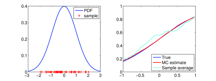
Figure 1: Toy example to compare the Monte Carlo method and sample average. (a) 30 i.i.d. sample points from a standard normal distribution. (b) Cumulative distribution functions of true model (blue), estimated using Monte Carlo method (red), and estimated using the sample average (cyan) in the range [-1, 1]. (c) Quantile values at 25%, 50%, and 75% of true and two estimate methods.

To illustrate the benefit in estimation accuracy via model-based procedures, we may compare the Monte Carlo (MC) method with the simple sample average approach. A toy example is shown in Fig. 1, where we generate 30 i.i.d. sample points from a standard normal distribution (Fig. 1a). In the MC method, we estimate mean and standard deviation from the sample, and then generate 2000 Monte Carlo sampling points to estimate the cumulative distribution within [-1,1]. In contrast, the sample average method estimates the cumulative distribution with the empirical distribution of the 30 points. This comparison is shown in Fig. 1b. Moreover, we compare the true and estimated quantiles at 25%, 50%, and 75% in Fig. 1c. It is apparent that the MC method provides more accurate and robust result.

To begin with, we provide a general definition of depth by considering it as a functional of the underlying data generating model. Then, we provide a two-stage estimation procedure for the depth via Monte Carlo sampling. In the rest of the paper, we primarily focus on functional data for illustration, and the development naturally applies to finite-dimensional data.

2.1 Depths within statistical models

Let 𝒫={θ:θΘ}𝒫conditional-setsubscript𝜃𝜃Θ\mathcal{P}=\{\mathbb{P}_{\theta}:\,\theta\in\Theta\} be a family of probability measures indexed by a parameter θ𝜃\theta over a function (vector) space 2([0,1]):={f:[0,1]:f22=01f2(x)dx<}\mathcal{F}\subset\mathcal{L}_{2}([0,1]):\,=\{f:\,[0,1]\to\mathbb{R}:\,\|f\|_{2}^{2}=\int_{0}^{1}f^{2}(x)\,dx<\infty\}. For example, θsubscript𝜃\mathbb{P}_{\theta} can be the measure of a Gaussian Process GP(m,C)𝑚𝐶(m,C) with parameter θ=(m,C)𝜃𝑚𝐶\theta=(m,C) collecting the mean function m:[0,1]:𝑚01m:\,[0,1]\to\mathbb{R} and the covariance function C:[0,1]×[0,1]:𝐶0101C:\,[0,1]\times[0,1]\to\mathbb{R}. Statistical depth should quantify how large a particular observed trajectory fobssubscript𝑓𝑜𝑏𝑠f_{obs}\in\mathcal{F} deviates from certain notion of center fcsubscript𝑓𝑐f_{c}\in\mathcal{F} under θsubscript𝜃\mathbb{P}_{\theta}. For example, in the case of the Gaussian Process (GP), a natural choice of the center would be its mean function.

2.1.1 Definitions of Depths

We will now provide the formal definition of a model-based functional depth, as well as the associated depth contour and central region. All these statistical terms can be considered as infinite-dimensional generalization of the uni-variate survival function/p𝑝p-value, quantiles, and highest-probability region.

Our proposed definition can be either norm-based or inner-product based. We refer to the norm or inner-product as the criterion in the definition. The norm-based depth is a generalization over various distance-based forms (see the discussion after the following definition). In contrast, the inner-product depth is motivated with the classical halfspace depth by Tukey (1975). We at first define the norm-based depth in the following general form:

Definition 1.

(Norm-based statistical depth: general form): The statistical depth Dngsubscript𝐷𝑛𝑔D_{ng} of fobssubscript𝑓𝑜𝑏𝑠f_{obs}\in\mathcal{F} in the model θ𝒫subscript𝜃𝒫\mathbb{P}_{\theta}\in\mathcal{P} relative to the norm \|\cdot\| and center fcsubscript𝑓𝑐f_{c}\in\mathcal{F} is defined as

Dng(fobs,θ,,fc)[0,1],\displaystyle D_{ng}(f_{obs},\,\mathbb{P}_{\theta},\|\cdot\|,f_{c})\in[0,1],

where Dngsubscript𝐷𝑛𝑔D_{ng} is strictly decreasing with respect to fobsfcnormsubscript𝑓𝑜𝑏𝑠subscript𝑓𝑐\|f_{obs}-f_{c}\|, and Dng0subscript𝐷𝑛𝑔0D_{ng}\rightarrow 0 when fobsfcnormsubscript𝑓𝑜𝑏𝑠subscript𝑓𝑐\|f_{obs}-f_{c}\|\rightarrow\infty.

Norm-based depths are commonly used in statistics literature. For example, the hh-depth (Nieto-Reyes, 2011) and spatial depth (Sguera et al., 2014) are based on the 𝕃2superscript𝕃2\mathbb{L}^{2} norm, the 𝕃psuperscript𝕃𝑝\mathbb{L}^{p}-depth is based on the 𝕃psuperscript𝕃𝑝\mathbb{L}^{p} norm (Zuo & Serfling, 2000; Long & Huang, 2015), and the Mahalanobis depth is based on the Mahalanobis norm (Liu et al., 1999). The depth in Definition 1 generalizes these concepts and provides a broader framework for norm-based methods. In this paper, we study one specific form of this general definition. This specific form more resembles conventional depths and satisfies more desirable mathematical properties. The norm in the definition can be considered as a criterion function to compute the distance between any observation fobssubscript𝑓𝑜𝑏𝑠f_{obs} and the center fcsubscript𝑓𝑐f_{c} and we denote the criterion function as ζ(fobs,fc)𝜁subscript𝑓𝑜𝑏𝑠subscript𝑓𝑐\zeta(f_{obs},f_{c}) in the rest.

Definition 2.

(Norm-based statistical depth: specific form): The statistical depth Dnsubscript𝐷𝑛D_{n} of fobssubscript𝑓𝑜𝑏𝑠f_{obs}\in\mathcal{F} in model θ𝒫subscript𝜃𝒫\mathbb{P}_{\theta}\in\mathcal{P} relative to norm \|\cdot\| and center fcsubscript𝑓𝑐f_{c}\in\mathcal{F} is defined as

Dn(fobs,θ,,fc):=θ[f:ffcfobsfc].\displaystyle D_{n}(f_{obs},\,\mathbb{P}_{\theta},\|\cdot\|,f_{c}):\,=\mathbb{P}_{\theta}\big{[}f\in\mathcal{F}:\|f-f_{c}\|\geq\|f_{obs}-f_{c}\|\big{]}.

Remark 1: We point out that this specific form of depth is a representative of all norm-based depth in the general form as defined in Definition 1. In fact, Dn(fobs)subscript𝐷𝑛subscript𝑓𝑜𝑏𝑠D_{n}(f_{obs}) measures the degree of extremeness of the observed function fobssubscript𝑓𝑜𝑏𝑠f_{obs}\in\mathcal{F} under any normal-based depth Dng(fobs)subscript𝐷𝑛𝑔subscript𝑓𝑜𝑏𝑠D_{ng}(f_{obs}) in the following sense,

θ[Dng(f)Dng(fobs)]=θ[Dn(f)Dn(fobs)]=θ[ffcfobsfc]=Dn(fobs).subscript𝜃delimited-[]subscript𝐷𝑛𝑔𝑓subscript𝐷𝑛𝑔subscript𝑓𝑜𝑏𝑠subscript𝜃delimited-[]subscript𝐷𝑛𝑓subscript𝐷𝑛subscript𝑓𝑜𝑏𝑠subscript𝜃delimited-[]norm𝑓subscript𝑓𝑐normsubscript𝑓𝑜𝑏𝑠subscript𝑓𝑐subscript𝐷𝑛subscript𝑓𝑜𝑏𝑠\displaystyle\mathbb{P}_{\theta}\big{[}D_{ng}(f)\leq D_{ng}(f_{obs})\big{]}=\mathbb{P}_{\theta}\big{[}D_{n}(f)\leq D_{n}(f_{obs})\big{]}=\mathbb{P}_{\theta}\big{[}\|f-f_{c}\|\geq\|f_{obs}-f_{c}\|\big{]}=D_{n}(f_{obs}).

Remark 2: One proper way to choose the center fcsubscript𝑓𝑐f_{c} is to minimize P(ffca)𝑃norm𝑓subscript𝑓𝑐𝑎P(\|f-f_{c}\|\geq a) for any given a>0𝑎0a>0. Note that

P(ffca)Effc2a2.𝑃norm𝑓subscript𝑓𝑐𝑎𝐸superscriptnorm𝑓subscript𝑓𝑐2superscript𝑎2P(\|f-f_{c}\|\geq a)\leq\frac{E\|f-f_{c}\|^{2}}{a^{2}}.

When the norm \|\cdot\| is inner-product induced (e.g. the classical 𝕃2superscript𝕃2\mathbb{L}^{2} norm), it is easy to know that the optimal fcsubscript𝑓𝑐f_{c} should be the expectation Ef𝐸𝑓Ef. However, fcsubscript𝑓𝑐f_{c} in general can take different form, dependent on different selection of the norm.

Based on the definitions of the norm-based depth, we can naturally introduce the notions of depth contour and central region as follows. We adopt the specific form in Definition 2 to simplify notation (same notion can be directly applied to the general form).

Definition 3.

(Depth contour and central region for norm-based depth): For any α[0,1]𝛼01\alpha\in[0,1], the α𝛼\alpha-th depth contour in the model θ𝒫subscript𝜃𝒫\mathbb{P}_{\theta}\in\mathcal{P} relative to the norm \|\cdot\| and center fcsubscript𝑓𝑐f_{c}\in\mathcal{F} is defined as

Cn(α,θ,,fc):={f:Dn(f,θ,,fc)=α}.\displaystyle C_{n}(\alpha,\,\mathbb{P}_{\theta},\|\cdot\|,f_{c}):\,=\big{\{}f\in\mathcal{F}:\,D_{n}(f,\,\mathbb{P}_{\theta},\|\cdot\|,f_{c})=\alpha\big{\}}.

Also, the α𝛼\alpha-th central region in the model θ𝒫subscript𝜃𝒫\mathbb{P}_{\theta}\in\mathcal{P} relative to the norm \|\cdot\| and center fcsubscript𝑓𝑐f_{c}\in\mathcal{F} is defined as

Rn(α,θ,,fc):={f:Dn(f,θ,,fc)α}.\displaystyle R_{n}(\alpha,\,\mathbb{P}_{\theta},\|\cdot\|,f_{c}):\,=\big{\{}f\in\mathcal{F}:\,D_{n}(f,\,\mathbb{P}_{\theta},\|\cdot\|,f_{c})\geq\alpha\big{\}}.

Based on the multivariate halfspace depth, we now define the inner-product-based depth. In contrast to the general and specific forms in the norm-based case, the inner-product-based norm is defined only in a specific form as follows.

Definition 4.

(Inner-product-based statistical depth): The statistical depth Dipsubscript𝐷𝑖𝑝D_{ip} of fobssubscript𝑓𝑜𝑏𝑠f_{obs}\in\mathcal{F} in the model θ𝒫subscript𝜃𝒫\mathbb{P}_{\theta}\in\mathcal{P} relative to the inner-product ,\left<\cdot,\cdot\right> and a subset 𝒢𝒢\mathcal{G} of \mathcal{F} is defined as

Dip(fobs,θ,,,𝒢):=infg𝒢,g=1θ[f:f,gfobs,g]\displaystyle D_{ip}(f_{obs},\,\mathbb{P}_{\theta},\left<\cdot,\cdot\right>,\mathcal{G}):\,=\inf_{g\in\mathcal{G},||g||=1}\mathbb{P}_{\theta}\big{[}f\in\mathcal{F}:\left<f,g\right>\geq\left<f_{obs},g\right>\big{]}

Remark 3: There are two apparent differences between Definitions 2 and 4: 1) Definition 2 depends on the center fcsubscript𝑓𝑐f_{c}, whereas Definition 4 is independent of it. However, we will point out in Section 2.1.2 that when the distribution function has a center under certain form of symmetry, this center should be the deepest point under Definition 4. 2) Definition 4 involves an infimum in order to match the half-region depth (López-Pintado & Romo, 2011) for finite-dimensional Euclidean data. Different from the usual half-region depth where 𝒢𝒢\mathcal{G} as the range of the infimum is taken as the entire function space \mathcal{F}, the following lemma shows that for infinite-dimensional functional data, 𝒢𝒢\mathcal{G} is necessary to be a proper (finite-dimensional) subset to avoid depth value degeneracy. A proof is provided in Appendix E.

Lemma 1.

Let Csubscript𝐶\mathbb{P}_{C} be the probability measure of a zero-mean Gaussian process GP(0,C)0𝐶(0,C), where the eigensystem {(λj,ϕj)}j=1superscriptsubscriptsubscript𝜆𝑗subscriptitalic-ϕ𝑗𝑗1\{(\lambda_{j},\phi_{j})\}_{j=1}^{\infty} of the covariance operator C𝐶C has infinite number of positive eigenvalues {λj}j=1superscriptsubscriptsubscript𝜆𝑗𝑗1\{\lambda_{j}\}_{j=1}^{\infty}. If ,\langle\cdot,\cdot\rangle is an inner-product over \mathcal{F} such that the P×P𝑃𝑃P\times P Gram matrix [ϕj,ϕk]j,k=1Psuperscriptsubscriptdelimited-[]subscriptitalic-ϕ𝑗subscriptitalic-ϕ𝑘𝑗𝑘1𝑃[\langle\phi_{j},\phi_{k}\rangle]_{j,k=1}^{P} of the first P𝑃P eigenfunctions {ϕj}j=1Psuperscriptsubscriptsubscriptitalic-ϕ𝑗𝑗1𝑃\{\phi_{j}\}_{j=1}^{P} is positive definite for any P𝑃P\in\mathbb{N}, then

Dip(f,C,,,)=0subscript𝐷𝑖𝑝𝑓subscript𝐶0D_{ip}(f,\mathbb{P}_{C},\left<\cdot,\cdot\right>,\mathcal{F})=0

almost surely for f𝑓absentf\in GP(0,C)0𝐶(0,C).

Remark 4: This lemma indicates that special attention is needed for defining an inner-product-based depth for infinite-dimensional space \mathcal{F}. Dutta et al. (2011) also observed this anomalous behavior of halfspace depth in infinite-dimensional spaces. As a consequence, the halfspace depth (where 𝒢=𝒢\mathcal{G}=\mathcal{F}) is only meaningful for finite-dimensional space. In contrast, the norm-based depth can be effective for both finite- or infinite-dimensional space. To have a proper inner-product-based depth, either \mathcal{F} itself is finite-dimensional, or we use a finite-dimensional subset 𝒢𝒢\mathcal{G} as shown in Definition 4.

Under this model-based framework, we can naturally estimate the proposed statistical depth D(fobs,θ,,fc)𝐷subscript𝑓𝑜𝑏𝑠subscript𝜃subscript𝑓𝑐D(f_{obs},\,\mathbb{P}_{\theta},\cdot,f_{c}) via the following two-stage procedure: 1. Find an estimate θ^^𝜃\widehat{\theta} of the parameter θ𝜃\theta; 2. Compute the estimated depth D(fobs,Pθ^,,fc)𝐷subscript𝑓𝑜𝑏𝑠subscript𝑃^𝜃subscript𝑓𝑐D(f_{obs},\,P_{\widehat{\theta}},\cdot,f_{c}) by either using a closed-from expression of the depth or by a Monte Carlo method for an approximation. For example, when θsubscript𝜃\mathbb{P}_{\theta} is a GP measure and the depth as a functional of parameter θ𝜃\theta may not admit a closed-form expression, we may resort to Monte Carlo method for estimating the depth. More details of the estimation will be provided in Appendix A in the supplementary material of the paper.

2.1.2 Mathematical Properties

Zuo & Serfling (2000) introduced a list of favorable mathematical properties to be satisfied by good multivariate statistical depths. Based on this, Nieto-Reyes et al. (2016) further explored the extensions of these properties for functional data. Gijbels et al. (2017) discussed these properties on commonly used methods such as the random Tukey depth, band depth, and spatial depth. In this part, we discuss these properties on our norm-based and inner-product based depths.

Before discussing basic properties of these two types depths, we need to clarify the concept of “halfspace” with the following definition:

Definition 5.

A closed halfspace Hh,gsubscript𝐻𝑔H_{h,g} for g,h𝑔g,h\in\mathcal{F} is defined in the form

Hh,g={f:fh,g0}.subscript𝐻𝑔conditional-set𝑓𝑓𝑔0H_{h,g}=\big{\{}f\in\mathcal{F}:\left<f-h,g\right>\geq 0\big{\}}.

To make the inner-product-based depth satisfy favorable properties, we need the following assumption on the “center” function fcsubscript𝑓𝑐f_{c}.

Assumption 1: The distribution θsubscript𝜃\mathbb{P}_{\theta} of a random function f𝑓f\in\mathcal{F} is halfspace symmetric, or H-symmetric, about a unique function fcsubscript𝑓𝑐f_{c}. That is, (fH)1/2𝑓𝐻12\mathbb{P}(f\in H)\geq 1/2 for every closed halfspace H𝐻H containing fcsubscript𝑓𝑐f_{c}. Moreover, we assume that (fH)<1/2𝑓𝐻12\mathbb{P}(f\in H)<1/2 for every closed halfspace H𝐻H that does not contain fcsubscript𝑓𝑐f_{c}.

Now we list four basic properties of the norm-based depth (Definition 2) and the inner-product-based depth (Definition 4), respectively, as following:

Norm-based depth:

  • P-1. (Linear invariance) Let θ,Fsubscript𝜃𝐹\mathbb{P}_{\theta,F} denote the distribution Pθsubscript𝑃𝜃P_{\theta} of a random variable F𝐹F\in\mathcal{F}. Then for any a{0}𝑎0a\in\mathbb{R}\setminus\{0\} and hh\in\mathcal{F},

    D(afobs+h,θ,aF+h,,afc+h)=D(fobs,θ,F,,fc).D(af_{obs}+h,\,\mathbb{P}_{\theta,aF+h},\|\cdot\|,af_{c}+h)=D(f_{obs},\,\mathbb{P}_{\theta,F},\|\cdot\|,f_{c}).
  • P-2. (Maximality at center) D(fc,θ,,fc)=supfobsD(fobs,θ,,fc)D(f_{c},\,\mathbb{P}_{\theta},\|\cdot\|,f_{c})=\sup_{f_{obs}\in\mathcal{F}}D(f_{obs},\,\mathbb{P}_{\theta},\|\cdot\|,f_{c}).

  • P-3. (Monotonicity with respect to the deepest point) Let the deepest function be fcsubscript𝑓𝑐f_{c}\in\mathcal{F}. Then for any fobssubscript𝑓𝑜𝑏𝑠f_{obs}\in\mathcal{F} and α(0,1)𝛼01\alpha\in(0,1), D(fobs,θ,,fc)D(fc+α(fobsfc),θ,,fc)D(f_{obs},\,\mathbb{P}_{\theta},\|\cdot\|,f_{c})\leq D(f_{c}+\alpha(f_{obs}-f_{c}),\,\mathbb{P}_{\theta},\|\cdot\|,f_{c}).

  • P-4. (Vanishing at infinity) D(fobs,θ,,fc)0D(f_{obs},\,\mathbb{P}_{\theta},\|\cdot\|,f_{c})\to 0 as fobsnormsubscript𝑓𝑜𝑏𝑠\|f_{obs}\|\to\infty.

Inner-product-based depth:

  • P-1’. (Linear invariance) Let θ,Fsubscript𝜃𝐹\mathbb{P}_{\theta,F} denote the distribution Pθsubscript𝑃𝜃P_{\theta} of a random variable F𝐹F\in\mathcal{F}. Then for any a{0}𝑎0a\in\mathbb{R}\setminus\{0\} and hh\in\mathcal{F},

    Dip(afobs+h,θ,aF+h,,,𝒢)=Dip(fobs,θ,F,,,𝒢).subscript𝐷𝑖𝑝𝑎subscript𝑓𝑜𝑏𝑠subscript𝜃𝑎𝐹𝒢subscript𝐷𝑖𝑝subscript𝑓𝑜𝑏𝑠subscript𝜃𝐹𝒢D_{ip}(af_{obs}+h,\,\mathbb{P}_{\theta,aF+h},\left<\cdot,\cdot\right>,\mathcal{G})=D_{ip}(f_{obs},\,\mathbb{P}_{\theta,F},\left<\cdot,\cdot\right>,\mathcal{G}).
  • P-2’. (Maximality at center) Dip(fc,θ,,,𝒢)=supfobsDip(fobs,θ,,,𝒢)subscript𝐷𝑖𝑝subscript𝑓𝑐subscript𝜃𝒢subscriptsupremumsubscript𝑓𝑜𝑏𝑠subscript𝐷𝑖𝑝subscript𝑓𝑜𝑏𝑠subscript𝜃𝒢D_{ip}(f_{c},\,\mathbb{P}_{\theta},\left<\cdot,\cdot\right>,\mathcal{G})=\sup_{f_{obs}\in\mathcal{F}}D_{ip}(f_{obs},\,\mathbb{P}_{\theta},\left<\cdot,\cdot\right>,\mathcal{G}).

  • P-3’. (Monotonicity with respect to the deepest point) Let the deepest function be fcsubscript𝑓𝑐f_{c}\in\mathcal{F}. Then for any fobssubscript𝑓𝑜𝑏𝑠f_{obs}\in\mathcal{F} and α(0,1)𝛼01\alpha\in(0,1), Dip(fobs,θ,,,𝒢)Dip(fc+α(fobsfc),θ,,,𝒢)subscript𝐷𝑖𝑝subscript𝑓𝑜𝑏𝑠subscript𝜃𝒢subscript𝐷𝑖𝑝subscript𝑓𝑐𝛼subscript𝑓𝑜𝑏𝑠subscript𝑓𝑐subscript𝜃𝒢D_{ip}(f_{obs},\,\mathbb{P}_{\theta},\left<\cdot,\cdot\right>,\mathcal{G})\leq D_{ip}(f_{c}+\alpha(f_{obs}-f_{c}),\,\mathbb{P}_{\theta},\left<\cdot,\cdot\right>,\mathcal{G}).

  • P-4’. (Vanishing at infinity) Dip(fobs,θ,,,𝒢)0subscript𝐷𝑖𝑝subscript𝑓𝑜𝑏𝑠subscript𝜃𝒢0D_{ip}(f_{obs},\,\mathbb{P}_{\theta},\left<\cdot,\cdot\right>,\mathcal{G})\to 0 as fobs,fobssubscript𝑓𝑜𝑏𝑠subscript𝑓𝑜𝑏𝑠\left<f_{obs},f_{obs}\right>\to\infty.

We examine these mathematical properties of the three defined depths in Sec. 2.1.1, as summarized in Lemma 2 below. The detailed proof is given in Appendix G.

Lemma 2.

The three depths in Definitions 1, 2, and 4 satisfy the mathematical properties given below:

  1. 1.

    Norm-based depth in general form (Definition 1): P-2, P-3, P-4.

  2. 2.

    Norm-based depth in specific form (Definition 2): P-1, P-2, P-3, P-4.

  3. 3.

    Inner-product-based depth (Definition 4, given Assumption 1): P-1’, P-2’, P-3’, P-4’.

2.2 Illustration of the Depth Definitions

We have defined two forms of model-based functional depth – norm-based (as in Definitions 1 and 2) and inner-product-based (as in Definition 4). In this section, we provide some examples, both finite-dimensional and infinite-dimensional, to illustrate these definitions. We will at first adopt various norms in Dnsubscript𝐷𝑛D_{n}, and then demonstrate the inner-product-based definition. Using these depths one can rank functional data based on their amplitude, continuity, smoothness, or phase variability. Moreover, we will show that some of the functional depths can also be directly applied to multivariate data.

2.2.1 Norm-based Depth

There are various norms on functional variables. One commonly used is the classical 𝕃psuperscript𝕃𝑝\mathbb{L}^{p}-norm, with p1𝑝1p\geq 1. That is, for f𝑓f in a proper space, its 𝕃psuperscript𝕃𝑝\mathbb{L}^{p}-norm is

fp=(01|f(t)|p𝑑t)1/p.subscriptnorm𝑓𝑝superscriptsuperscriptsubscript01superscript𝑓𝑡𝑝differential-d𝑡1𝑝\|f\|_{p}=(\int_{0}^{1}|f(t)|^{p}dt)^{1/p}.

In particular, 𝕃2superscript𝕃2\mathbb{L}^{2}-norm, the Euclidean distance from 0, is most often used in functional data analysis. Due to the nature of 𝕃2superscript𝕃2\mathbb{L}^{2} norm, it is a great tool for data visualization and ranking based on their own amplitude information. Considering functions in a Sobolev Space (Hsing & Eubank, 2015), we can also use 𝕃psuperscript𝕃𝑝\mathbb{L}^{p} norm on the derivatives functions to quantify continuity or smoothness feature. We may consider the norm-based depth in the following two forms:

  1. 1.

    Dn(fobs,θ,,fc):=θ[f:ffcpfobsfcp]D_{n}(f_{obs},\,\mathbb{P}_{\theta},\|\cdot\|,f_{c}):\,=\mathbb{P}_{\theta}\big{[}f\in\mathcal{F}:\|f-f_{c}\|_{p}\geq\|f_{obs}-f_{c}\|_{p}\big{]}

  2. 2.

    Dn(fobs,θ,,fc):=θ[f:DrfDrfcpDrfobsDrfcp]D_{n}(f_{obs},\,\mathbb{P}_{\theta},\|\cdot\|,f_{c}):\,=\mathbb{P}_{\theta}\big{[}f\in\mathcal{F}:\|D^{r}f-D^{r}f_{c}\|_{p}\geq\|D^{r}f_{obs}-D^{r}f_{c}\|_{p}\big{]}, where Drsuperscript𝐷𝑟D^{r} indicates r𝑟r-th order differentiation.

When we adopt the 𝕃psuperscript𝕃𝑝\mathbb{L}^{p} norm, the resulting depth can approxiamte band depth (López-Pintado & Romo, 2009) for functional observations from a distribution with mean 0.

In addition to having variability in amplitude (characterized by 𝕃psuperscript𝕃𝑝\mathbb{L}^{p} norms), functional observations often exhibit variability in phase. Such variability has been extensively studied over the past two decades and various methods were proposed to separate phase and amplitude, and quantify each variability in the given data (Ramsay & Li, 1998; Liu & Müller, 2004; Tang & Müller, 2008; Cleveland et al., 2018). In particular, phase is represented with time warping functions – Let ΓΓ\Gamma be the set of orientation-preserving diffeomorphisms of the unit interval [0,1]01[0,1]: Γ={γ:[0,1][0,1]|γ(0)=0,γ(1)=1,γ˙>0}Γconditional-set𝛾0101ketformulae-sequence𝛾00𝛾11˙𝛾0\Gamma=\{\gamma:[0,1]\to[0,1]|\gamma(0)=0,\gamma(1)=1,\dot{\gamma}>0\} (the dot indicates derivative operation), and γ𝛾\gamma is called a warping function. Given two functions u,v𝑢𝑣u,v, we denote γuvsubscript𝛾𝑢𝑣\gamma_{uv} as the optimal warping from u𝑢u to v𝑣v. There are various forms to define the “optimal” warping, and here we adopt the well-known Fisher-Rao framework (Srivastava et al., 2011) and

γuv=arginfγΓ(q(u)γ)γ˙q(v)2subscript𝛾𝑢𝑣subscriptarginf𝛾Γsubscriptnorm𝑞𝑢𝛾˙𝛾𝑞𝑣2\gamma_{uv}=\mbox{arginf}_{\gamma\in\Gamma}\|(q(u)\circ\gamma)\sqrt{\dot{\gamma}}-q(v)\|_{2}

where \circ denotes function composition and q()𝑞q(\cdot) is a transformation on the given function defined as q(x)=sign(x˙)|x˙|𝑞𝑥𝑠𝑖𝑔𝑛˙𝑥˙𝑥q(x)=sign(\dot{x})\sqrt{|\dot{x}|}. The degree of warpingness from the identity γid(t)=tsubscript𝛾𝑖𝑑𝑡𝑡\gamma_{id}(t)=t can be properly measured by two distances, namely, the 𝕃2superscript𝕃2\mathbb{L}^{2} distance and the Fisher-Rao distance. We may consider the norm criterion based on each of these distances:

  1. 1.

    Dn(fobs,θ,,fc):=θ[f:γffcγid2γfobsfcγid2]D_{n}(f_{obs},\,\mathbb{P}_{\theta},\|\cdot\|,f_{c}):\,=\mathbb{P}_{\theta}\big{[}f\in\mathcal{F}:\|\gamma_{ff_{c}}-\gamma_{id}\|_{2}\geq\|\gamma_{f_{obs}f_{c}}-\gamma_{id}\|_{2}\big{]}

  2. 2.

    Dn(fobs,θ,,fc):=θ[f:dFR(γffc,γid)dFR(γfobsfc,γid)]D_{n}(f_{obs},\,\mathbb{P}_{\theta},\|\cdot\|,f_{c}):\,=\mathbb{P}_{\theta}\big{[}f\in\mathcal{F}:d_{FR}(\gamma_{ff_{c}},\gamma_{id})\geq d_{FR}(\gamma_{f_{obs}f_{c}},\gamma_{id})\big{]}, where dFR(γuv,γid)=cos1(01γ˙uv(t)γ˙id(t)𝑑t)=cos1(01γ˙uv(t)𝑑t),subscript𝑑𝐹𝑅subscript𝛾𝑢𝑣subscript𝛾𝑖𝑑𝑐𝑜superscript𝑠1superscriptsubscript01subscript˙𝛾𝑢𝑣𝑡subscript˙𝛾𝑖𝑑𝑡differential-d𝑡𝑐𝑜superscript𝑠1superscriptsubscript01subscript˙𝛾𝑢𝑣𝑡differential-d𝑡d_{FR}(\gamma_{uv},\gamma_{id})=cos^{-1}(\int_{0}^{1}\sqrt{\dot{\gamma}_{uv}(t)}\sqrt{\dot{\gamma}_{id}(t)}dt)=cos^{-1}(\int_{0}^{1}\sqrt{\dot{\gamma}_{uv}(t)}dt),

Due to the nature of the Fisher-Rao distance, depth based on this criteria in our framework is sensitive to smoothness in the warping function.

2.2.2 Inner-product-based Depth

For multivariate data, Tukey’s halfspace depth (Tukey, 1975) is one of the most popular depth functions available in literature. Dutta et al. (2011) investigated an extension on any Banach space, and proposed a specialization on a Hilbert space \mathcal{H}. If X is a random element in \mathcal{H} having the distribution F𝐹F, then the halfspace depth of an observation x𝑥x\in\mathcal{H} is defined as

HD(x,F)=infhP{h,Xx0},𝐻𝐷𝑥𝐹subscriptinfimum𝑃X𝑥0HD(x,F)=\inf_{h\in\mathcal{H}}P\{\left<h,\textbf{X}-x\right>\geq 0\},

where ,\left<\cdot,\cdot\right> stands for the inner product defined on \mathcal{H}. Note that the inner-product based depth in Definition 4 can be rewritten as

Dip(fobs,θ,,,𝒢):=infg𝒢,g=1θ[f:f,gfobs,g]=infg𝒢,g=1θ[ffobs,g0].D_{ip}(f_{obs},\,\mathbb{P}_{\theta},\left<\cdot,\cdot\right>,\mathcal{G}):\,=\inf_{g\in\mathcal{G},||g||=1}\mathbb{P}_{\theta}\big{[}f\in\mathcal{F}:\left<f,g\right>\geq\left<f_{obs},g\right>\big{]}=\inf_{g\in\mathcal{G},||g||=1}\mathbb{P}_{\theta}\big{[}\left<f-f_{obs},g\right>\geq 0\big{]}.

Therefore, the halfspace depth can be treated as one special case in the proposed framework. However, Lemma 1 illustrates that the halfspace depth may collapse to zero for infinite-dimensional functional data unless the underlying data generating model is intrinsically finite-dimensional. As a consequence, the choice of the range 𝒢𝒢\mathcal{G} of the infimum in the preceding display becomes important.

In general, there is no simple solution to the above minimization process (Tukey, 1975; Rousseeuw & Ruts, 1996; Dutta et al., 2011). However, if the functions are samples from a finite-dimensional stochastic process, an optimal g𝑔g can be found in closed forms. For illustration purpose, let us assume that the data generating process is a finite-dimensional Gaussian process. Then the minimization takes the the following closed-form (see detailed derivation in Appendix F)

Dip(fobs)=1Φ(fobsK),subscript𝐷𝑖𝑝subscript𝑓𝑜𝑏𝑠1Φsubscriptnormsubscript𝑓𝑜𝑏𝑠subscript𝐾D_{ip}(f_{obs})=1-\Phi(\|f_{obs}\|_{\mathbb{H}_{K}}),

where ΦΦ\Phi is the c.d.f. of a standard normal random variable and the norm K\|\cdot\|_{\mathbb{H}_{K}} is the induced RKHS norm (formal definitions are provided in Section 3). Note that as ΦΦ\Phi is a c.d.f. function, the depth value of fobssubscript𝑓𝑜𝑏𝑠f_{obs} is in the range [0,1/2]012[0,1/2], which is consistent to the notion of halfspace depth in function space (Dutta et al., 2011). It is well known that, for the halfspace depth, if we have a symmetric distribution in a Hilbert space, then the maximum depth is 0.50.50.5, and the point of symmetry will achieve at the halfspace median. In this case, it is easy to see that Dip(fobs)=1/2fobs=0subscript𝐷𝑖𝑝subscript𝑓𝑜𝑏𝑠12subscript𝑓𝑜𝑏𝑠0D_{ip}(f_{obs})=1/2\Leftrightarrow f_{obs}=0. Therefore, the median (i.e. function with largest depth value) is our center function fc=0subscript𝑓𝑐0f_{c}=0.

Remark 5: The above result is based on the assumption that the stochastic process is a Gaussian process. However, the Gaussianity is only used in the step that the c.d.f. ΦΦ\Phi is independent of g𝑔g after the standardization (i.e., XXμgσg𝑋𝑋subscript𝜇𝑔subscript𝜎𝑔X\rightarrow\frac{X-\mu_{g}}{\sigma_{g}}), and the results can be generalized to any second-order stochastic process.

Simplifications in Multivariate Data: The above inner-product-based depth can also be applied to multivariate data where the Gaussian process reduces to a multivariate Gaussian distribution, denoted as 𝒩(μ,Σ)𝒩𝜇Σ\mathcal{N}(\mu,\Sigma). In particular, the corresponding inner-product criterion function reduces to a variant of the well-known Tukey’s halfspace depth, or location depth (Tukey, 1975),

Dip(x)=infud,u=1P{X:u,Xx0},subscript𝐷𝑖𝑝𝑥subscriptinfimumformulae-sequence𝑢superscript𝑑norm𝑢1𝑃conditional-set𝑋𝑢𝑋𝑥0D_{ip}(x)=\inf_{u\in\mathbb{R}^{d},\,\|u\|=1}P\{X:\langle u,X-x\rangle\geq 0\},

where the new halfspace depth incorporates the second moment information ΣΣ\Sigma through the (zero-mean) inner product x,y=xTΣ1y𝑥𝑦superscript𝑥𝑇superscriptΣ1𝑦\left<x,y\right>=x^{T}\Sigma^{-1}y and the norm x2=xTΣ1xsuperscriptnorm𝑥2superscript𝑥𝑇superscriptΣ1𝑥\|x\|^{2}=x^{T}\Sigma^{-1}x induced from the covariance matrix of the multivariate data generating distribution, and 𝒢𝒢\mathcal{G} becomes the unit ball of dsuperscript𝑑\mathbb{R}^{d} relative to this inner-product. In the special case when X𝑋X is a random realization from a zero-mean multivariate normal distribution, or X𝒩(0,Σ)similar-to𝑋𝒩0ΣX\sim\mathcal{N}(0,\Sigma), then the half-space depth Dipsubscript𝐷𝑖𝑝D_{ip} admits a closed form. More concretely, using the singular value decomposition on the covariance matrix Σ=UΛUTΣ𝑈Λsuperscript𝑈𝑇\Sigma=U\Lambda U^{T}, where ΛΛ\Lambda is a diagonal matrix with elements of eigenvalues {λp}p=1dsuperscriptsubscriptsubscript𝜆𝑝𝑝1𝑑\{\lambda_{p}\}_{p=1}^{d}, we can express X𝑋X through a finite-dimensional version of the Karhunen Loève expansion X=p=1dξpUp𝑋superscriptsubscript𝑝1𝑑subscript𝜉𝑝subscript𝑈𝑝X=\sum_{p=1}^{d}\xi_{p}U_{p}, where Upsubscript𝑈𝑝U_{p} is the p𝑝p-th column of U𝑈U (i.e. the eigenvector corresponding to λpsubscript𝜆𝑝\lambda_{p}), and ξp𝒩(0,λp)similar-tosubscript𝜉𝑝𝒩0subscript𝜆𝑝\xi_{p}\sim\mathcal{N}(0,\lambda_{p}), p=1,2,,d𝑝12𝑑p=1,2,\ldots,d are independent random variables. Correspondingly, the depth of any xd𝑥superscript𝑑x\in\mathbb{R}^{d} is given as

Dip(x)=1Φ(p=1dξp2λp).subscript𝐷𝑖𝑝𝑥1Φsuperscriptsubscript𝑝1𝑑superscriptsubscript𝜉𝑝2subscript𝜆𝑝D_{ip}(x)=1-\Phi(\sqrt{\sum_{p=1}^{d}\frac{\xi_{p}^{2}}{\lambda_{p}}}).

Note that the maximum depth value computed by this way is the same as maximum via Tukey’s half space depth, which is 1/2121/2.

3 A New Model-Based Depth for Functional Data

In this section, we apply our proposed depth framework to functional data and propose a new data-dependent functional depth. As we will illustrate, our new model-based functional depths can capture and adapt to global features such as smoothness and shapes in the underlying data generating processes. Our proposed methods incorporate information from the reproducing kernel Hilbert space (RKHS) associated with the covariance operator of the underlying stochastic process.

3.1 Depths induced by reproducing kernels

We will provide a construction of norm-based depth for zero-mean second-order stochastic processes \mathcal{F}, where the norm itself is model-dependent and learned from the data. Recall that a stochastic process {f(t):t[0,1]}conditional-set𝑓𝑡𝑡01\{f(t):\,t\in[0,1]\} is a second-order process if 𝔼[f2(t)]<𝔼delimited-[]superscript𝑓2𝑡\mathbb{E}[f^{2}(t)]<\infty for all t[0,1]𝑡01t\in[0,1], so that its covariance function 𝔼[f(s)f(t)]𝔼delimited-[]𝑓𝑠𝑓𝑡\mathbb{E}[f(s)f(t)] is well-defined. If the process has a nonzero mean function m𝑚m, then we can always subtract the mean by choosing the center fcsubscript𝑓𝑐f_{c} as m𝑚m.

3.1.1 Background on covariance kernels

Since {f(t):t[0,1]}conditional-set𝑓𝑡𝑡01\{f(t):\,t\in[0,1]\} is a second-order process, its covariance kernel K[0,1]×[0,1]𝐾0101maps-toK\in[0,1]\times[0,1]\mapsto\mathbb{R}, K(s,t):=𝔼[f(s)f(t)]assign𝐾𝑠𝑡𝔼delimited-[]𝑓𝑠𝑓𝑡K(s,t):=\mathbb{E}[f(s)f(t)] is a well-defined function for all (s,t)[0,1]2𝑠𝑡superscript012(s,t)\in[0,1]^{2}. In addition, K(,)𝐾K(\cdot,\cdot) is a symmetric, positive semi-definite real-value function, that is,

i)\displaystyle i) K(s,t)=K(t,s),𝐾𝑠𝑡𝐾𝑡𝑠\displaystyle\ \ \ \ K(s,t)=K(t,s),
ii)\displaystyle ii) 0101K(s,t)h(s)h(t)𝑑s𝑑t0for any h.superscriptsubscript01superscriptsubscript01𝐾𝑠𝑡𝑠𝑡differential-d𝑠differential-d𝑡0for any h\displaystyle\ \ \ \int_{0}^{1}\int_{0}^{1}K(s,t)\,h(s)\,h(t)\,ds\,dt\geq 0\ \text{for any $h\in\mathcal{F}$}.

According to Mercer’s Theorem (J Mercer, 1909), there exists a sequence of orthonormal eigenfunctions {ϕ1(t),ϕ2(t),}subscriptitalic-ϕ1𝑡subscriptitalic-ϕ2𝑡\{\phi_{1}(t),\phi_{2}(t),\cdots\} over [0,1]01[0,1] and a sequence of corresponding non-negative eigenvalues λ1λ20subscript𝜆1subscript𝜆20\lambda_{1}\geq\lambda_{2}\geq\cdots\geq 0 (Riesz & Nagy, 1990) satisfying

01K(s,t)ϕp(s)𝑑s=λpϕp(t),for any p1,  and K(s,t)=p=1λpϕp(s)ϕp(t),formulae-sequencesuperscriptsubscript01𝐾𝑠𝑡subscriptitalic-ϕ𝑝𝑠differential-d𝑠subscript𝜆𝑝subscriptitalic-ϕ𝑝𝑡for any p1,  and 𝐾𝑠𝑡superscriptsubscript𝑝1subscript𝜆𝑝subscriptitalic-ϕ𝑝𝑠subscriptitalic-ϕ𝑝𝑡\displaystyle\int_{0}^{1}K(s,t)\phi_{p}(s)ds=\lambda_{p}\phi_{p}(t),\ \text{for any $p\geq 1$, \ and \ }K(s,t)=\sum_{p=1}^{\infty}\lambda_{p}\phi_{p}(s)\phi_{p}(t), (1)

which implies 0101K2(s,t)𝑑s𝑑t=p=1λp2superscriptsubscript01superscriptsubscript01superscript𝐾2𝑠𝑡differential-d𝑠differential-d𝑡superscriptsubscript𝑝1superscriptsubscript𝜆𝑝2\int_{0}^{1}\int_{0}^{1}K^{2}(s,t)\,ds\,dt=\sum_{p=1}^{\infty}\lambda_{p}^{2}. The convergence in Equation (1) is absolute and uniform on [0,1]×[0,1]0101[0,1]\times[0,1] (Cucker & Zhou, 2007).

By the Karhunen Loève theorem (Ash, 1990), a random observation f𝑓f has the following representation

f(t)=p=1fpϕp(t)𝑓𝑡superscriptsubscript𝑝1subscript𝑓𝑝subscriptitalic-ϕ𝑝𝑡\displaystyle f(t)=\sum_{p=1}^{\infty}f_{p}\phi_{p}(t) (2)

where f1,f2,subscript𝑓1subscript𝑓2f_{1},f_{2},\cdots are uncorrelated random variables with mean 𝔼fp=0𝔼subscript𝑓𝑝0\mathbb{E}f_{p}=0, and variance 𝔼fp2=λp𝔼superscriptsubscript𝑓𝑝2subscript𝜆𝑝\mathbb{E}f_{p}^{2}=\lambda_{p}. Each coefficient fpsubscript𝑓𝑝f_{p} is unique and can be obtained by fp=01f(s)ϕp(s)𝑑s.subscript𝑓𝑝superscriptsubscript01𝑓𝑠subscriptitalic-ϕ𝑝𝑠differential-d𝑠f_{p}=\int_{0}^{1}f(s)\phi_{p}(s)ds. In particular, if the stochastic process is a GP, f1,f2,subscript𝑓1subscript𝑓2f_{1},f_{2},\cdots will be independent Gaussian random variables.

3.1.2 Reproducing kernel Hilbert space and its induced norm

Any symmetric, positive semi-definite function K𝐾K on [0,1]×[0,1]0101[0,1]\times[0,1] corresponds to a unique RKHS with K𝐾K as its reproducing kernel (Wahba, 1990). We denote this RKHS by Ksubscript𝐾\mathbb{H}_{K} with inner-product

K(s,),K(t,)K=K(t,),K(s,)K=K(s,t).subscript𝐾𝑠𝐾𝑡subscript𝐾subscript𝐾𝑡𝐾𝑠subscript𝐾𝐾𝑠𝑡\displaystyle\langle K(s,\cdot),K(t,\cdot)\rangle_{\mathbb{H}_{K}}=\langle K(t,\cdot),K(s,\cdot)\rangle_{\mathbb{H}_{K}}=K(s,t).

Moreover, the reproducing property ensures that for any fK𝑓subscript𝐾f\in\mathbb{H}_{K}, f,K(t,)K=f(t)subscript𝑓𝐾𝑡subscript𝐾𝑓𝑡\langle f,K(t,\cdot)\rangle_{\mathbb{H}_{K}}=f(t). The inner product induces the RKHS norm fK=f,fKsubscriptnorm𝑓subscript𝐾subscript𝑓𝑓subscript𝐾\|f\|_{\mathbb{H}_{K}}=\sqrt{\langle f,\,f\rangle_{\mathbb{H}_{K}}}. This leads to an equivalent definition of the RKHS as K={f:[0,1],fK<}subscript𝐾conditional-set𝑓formulae-sequence01subscriptnorm𝑓subscript𝐾\mathbb{H}_{K}=\{f:\,[0,1]\to\mathbb{R},\,\|f\|_{\mathbb{H}_{K}}<\infty\}. Therefore, under the representations in Equations  (1) and (2), we have fK𝑓subscript𝐾f\in\mathbb{H}_{K} if and only if fK2=p:λp>0fp2λp<superscriptsubscriptnorm𝑓subscript𝐾2subscript:𝑝subscript𝜆𝑝0superscriptsubscript𝑓𝑝2subscript𝜆𝑝\|f\|_{\mathbb{H}_{K}}^{2}=\sum_{p:\lambda_{p}>0}\frac{f_{p}^{2}}{\lambda_{p}}<\infty.

For a random trajectory f𝑓f\in\mathcal{F} from a second-order stochastic process with covariance kernel K𝐾K, it is important to examine if the norm fK2superscriptsubscriptnorm𝑓subscript𝐾2\|f\|_{\mathbb{H}_{K}}^{2} is finite. If K𝐾K has only finite number of positive eigenvalues, this conclusion certainly holds. However, if K𝐾K has infinite number of positive eigenvalues, in general p:λp>0fp2λp=(a.s.)\sum_{p:\lambda_{p}>0}\frac{f_{p}^{2}}{\lambda_{p}}=\infty(a.s.) since by the SLLN,

1np=1nfp2λpa.s.E(fp2λp)=1\frac{1}{n}\sum_{p=1}^{n}\frac{f_{p}^{2}}{\lambda_{p}}\overset{a.s.}{\longrightarrow}E(\frac{f_{p}^{2}}{\lambda_{p}})=1

(the case for GP is discussed in (Wahba, 1990)).

Consequently, although the RKHS norm K\|\cdot\|_{\mathbb{H}_{K}} contains important global features of the underlying data generating process, we cannot use the RKHS norm to define the depth since the RKHS norm of the observations are infinite almost surely. For example, for one-dimensional integrated Bownian motions (Vaart & Zanten, 2011), it is known that smoothness level of the sample trajectories is 0.50.50.5 smaller than that of its associated RKHS (for Brownian motion, see (Karatzas & Shreve, 2012)), where the corresponding RKHS norm coincides with the Sobolev norm. In this paper, we aim to combine these global features reflected in the RKHS norm into the construction of model-based functional depth. In particular, to solve this divergent issue of the RKHS norm, we propose a modified RKHS norm in the construction of our norm induced depth for functional data by weakening the impact of high-frequency signals, which are usually hard to estimate, on the modified norm.

3.2 Depth induced by modified RKHS norm

In this section, we propose a modified inner product structure for functions in \mathcal{F}. This new inner product will induce a modified RKHS norm that is almost surely finite for the sample trajectories from the second-order stochastic process.

3.2.1 Modified Inner Product and Norm

Suppose f,g𝑓𝑔f,g are two random realizations over \mathcal{F} from a second-order stochastic process with covariance kernel K𝐾K. Recall the eigen-decomposition K(s,t)=p=1λpϕp(s)ϕp(t)𝐾𝑠𝑡superscriptsubscript𝑝1subscript𝜆𝑝subscriptitalic-ϕ𝑝𝑠subscriptitalic-ϕ𝑝𝑡K(s,t)=\sum_{p=1}^{\infty}\lambda_{p}\phi_{p}(s)\phi_{p}(t) for any s,t[0,1]𝑠𝑡01s,t\in[0,1]. Without loss of generality, we assume all eigenvalues {λp}subscript𝜆𝑝\{\lambda_{p}\} are positive to avoid zero appearing in the denominator.

Recall the Karhunen Loève expansion, f(t)=p=1fpϕp(t)𝑓𝑡superscriptsubscript𝑝1subscript𝑓𝑝subscriptitalic-ϕ𝑝𝑡f(t)=\sum_{p=1}^{\infty}f_{p}\phi_{p}(t) and g(t)=p=1gpϕp(t)𝑔𝑡superscriptsubscript𝑝1subscript𝑔𝑝subscriptitalic-ϕ𝑝𝑡g(t)=\sum_{p=1}^{\infty}g_{p}\phi_{p}(t), with fp=01f(s)ϕp(s)𝑑ssubscript𝑓𝑝superscriptsubscript01𝑓𝑠subscriptitalic-ϕ𝑝𝑠differential-d𝑠f_{p}=\int_{0}^{1}f(s)\phi_{p}(s)ds and gp=01g(s)ϕp(s)𝑑ssubscript𝑔𝑝superscriptsubscript01𝑔𝑠subscriptitalic-ϕ𝑝𝑠differential-d𝑠g_{p}=\int_{0}^{1}g(s)\phi_{p}(s)ds. In addition, the RKHS induced inner-product and norm are given in the following forms, respectively.

f,gK=p=1fpgpλpandf=f,fK1/2formulae-sequencesubscript𝑓𝑔subscript𝐾superscriptsubscript𝑝1subscript𝑓𝑝subscript𝑔𝑝subscript𝜆𝑝andnorm𝑓superscriptsubscript𝑓𝑓subscript𝐾12\displaystyle\langle f,g\rangle_{\mathbb{H}_{K}}=\sum_{p=1}^{\infty}\frac{f_{p}g_{p}}{\lambda_{p}}\ \ \mbox{and}\ \ \|f\|=\langle f,f\rangle_{\mathbb{H}_{K}}^{1/2}

As we discussed earlier in Sec. 3.1, the RKHS norm diverges almost surely. This divergence motivates us to a modified inner-product as follows:

f,gmod:=p=1fpgpλpap2assignsubscript𝑓𝑔𝑚𝑜𝑑superscriptsubscript𝑝1subscript𝑓𝑝subscript𝑔𝑝subscript𝜆𝑝superscriptsubscript𝑎𝑝2\displaystyle\langle f,g\rangle_{mod}:=\sum_{p=1}^{\infty}\frac{f_{p}g_{p}}{\lambda_{p}}a_{p}^{2}

where {ap}p=1superscriptsubscriptsubscript𝑎𝑝𝑝1\{a_{p}\}_{p=1}^{\infty} is any real sequence satisfying p=1ap2<superscriptsubscript𝑝1superscriptsubscript𝑎𝑝2\sum_{p=1}^{\infty}a_{p}^{2}<\infty. In practice, we may adopt commonly used convergent sequence {ap=1ps}p=1superscriptsubscriptsubscript𝑎𝑝1superscript𝑝𝑠𝑝1\{a_{p}=\frac{1}{p^{s}}\}_{p=1}^{\infty} or {ap=1p(logp)s}p=1superscriptsubscriptsubscript𝑎𝑝1𝑝superscript𝑝𝑠𝑝1\{a_{p}=\frac{1}{\sqrt{p}(\log p)^{s}}\}_{p=1}^{\infty}with s>1/2𝑠12s>1/2. Our idea is to assign a decaying weight to each positive eigenvalue, so that the overall sum converges after the adjustment. This modified inner product yields a squared modified RKHS norm as

fmod2=f,fmod=p=1fp2λpap2.superscriptsubscriptnorm𝑓𝑚𝑜𝑑2subscript𝑓𝑓𝑚𝑜𝑑superscriptsubscript𝑝1superscriptsubscript𝑓𝑝2subscript𝜆𝑝superscriptsubscript𝑎𝑝2\displaystyle\|f\|_{mod}^{2}=\langle f,f\rangle_{mod}=\sum_{p=1}^{\infty}\frac{f_{p}^{2}}{\lambda_{p}}a_{p}^{2}.

Straightforward calculations yield 𝔼(fmod2)=p=1E(fp2)λpap2=p=1ap2<𝔼superscriptsubscriptnorm𝑓𝑚𝑜𝑑2superscriptsubscript𝑝1𝐸superscriptsubscript𝑓𝑝2subscript𝜆𝑝superscriptsubscript𝑎𝑝2superscriptsubscript𝑝1superscriptsubscript𝑎𝑝2\mathbb{E}(\|f\|_{mod}^{2})=\sum_{p=1}^{\infty}\frac{E(f_{p}^{2})}{\lambda_{p}}a_{p}^{2}=\sum_{p=1}^{\infty}a_{p}^{2}<\infty. As a consequence, fmod<subscriptnorm𝑓𝑚𝑜𝑑\|f\|_{mod}<\infty almost surely, and the above modified inner product and norm are well-defined for the observed trajectories. We can use this modified RKHS norm to define a model-based norm-induced depth as described in Section 5.1.

Recall of Definition 2 of depth in Sec. 2.1: D(fobs,θ,,fc)=θ[ffcfobsfc]D(f_{obs},\,\mathbb{P}_{\theta},\|\cdot\|,f_{c})=\mathbb{P}_{\theta}\big{[}\|f-f_{c}\|\geq\|f_{obs}-f_{c}\|\big{]}. In this case, the central function fc=0subscript𝑓𝑐0f_{c}=0 is the mean function in our model; the norm function is the modified RKHS norm =mod\|\cdot\|=\|\cdot\|_{mod}; θsubscript𝜃\mathbb{P}_{\theta} is a probability measure defined by the probability density on fmodsubscriptnorm𝑓𝑚𝑜𝑑\|f\|_{mod} or fmod2superscriptsubscriptnorm𝑓𝑚𝑜𝑑2\|f\|_{mod}^{2}. Apparently, with different settings of the decaying sequence {ap}p=1superscriptsubscriptsubscript𝑎𝑝𝑝1\{a_{p}\}_{p=1}^{\infty}, we will have different probability density for fmodsubscriptnorm𝑓𝑚𝑜𝑑\|f\|_{mod} or fmod2superscriptsubscriptnorm𝑓𝑚𝑜𝑑2\|f\|_{mod}^{2}. It is often intractable to derive a closed-from expression on the density. Fortunately, our model-based depth framework provides a natural way of estimating the depth through Monte Carlo sampling, where the coefficients ({fp}subscript𝑓𝑝\{f_{p}\} in the Karhunen-Loève expansion) can be simulated with re-sampling techniques such as the Bootstrap.

3.2.2 Depth estimation procedure and algorithm

Suppose we have n𝑛n zero-mean independent sample functions f1,,fnsubscript𝑓1subscript𝑓𝑛f_{1},\cdots,f_{n}\in\mathcal{F} on t[0,1]𝑡01t\in[0,1], and our goal is to compute the model-based depth of any observed sample fobssubscript𝑓𝑜𝑏𝑠f_{obs}\in\mathcal{F}. We propose an estimation algorithm as follows.

Algorithm I. (Input: functional data {f1,,fn}subscript𝑓1subscript𝑓𝑛\{f_{1},\cdots,f_{n}\}, any observation fobssubscript𝑓𝑜𝑏𝑠f_{obs}, a small threshold δn>0subscript𝛿𝑛0\delta_{n}>0, and a sequence a1,,ansubscript𝑎1subscript𝑎𝑛a_{1},\cdots,a_{n}.)

  1. 1.

    Compute the sample mean function f^(t)=1ni=1nfi(t)^𝑓𝑡1𝑛superscriptsubscript𝑖1𝑛subscript𝑓𝑖𝑡\hat{f}(t)=\frac{1}{n}\sum_{i=1}^{n}f_{i}(t), and empirical covariance kernel K^(s,t)=1ni=1n[fi(s)f^(s)][fi(t)f^(t)]^𝐾𝑠𝑡1𝑛superscriptsubscript𝑖1𝑛delimited-[]subscript𝑓𝑖𝑠^𝑓𝑠delimited-[]subscript𝑓𝑖𝑡^𝑓𝑡\hat{K}(s,t)=\frac{1}{n}\sum_{i=1}^{n}[f_{i}(s)-\hat{f}(s)][f_{i}(t)-\hat{f}(t)];

  2. 2.

    Eigen-decompose K^=p=1nλ^p,nϕ^p,n(s)ϕ^p,n(t)^𝐾superscriptsubscript𝑝1𝑛subscript^𝜆𝑝𝑛subscript^italic-ϕ𝑝𝑛𝑠subscript^italic-ϕ𝑝𝑛𝑡\hat{K}=\sum_{p=1}^{n}\hat{\lambda}_{p,n}\hat{\phi}_{p,n}(s)\hat{\phi}_{p,n}(t);

  3. 3.

    Set λ^p,n=0subscript^𝜆𝑝𝑛0\hat{\lambda}_{p,n}=0 if λ^p,n<δnsubscript^𝜆𝑝𝑛subscript𝛿𝑛\hat{\lambda}_{p,n}<\delta_{n};

  4. 4.

    Set Mn=argmaxm{λ^m,nδn}subscript𝑀𝑛subscriptargmax𝑚subscript^𝜆𝑚𝑛subscript𝛿𝑛M_{n}=\operatorname*{arg\ max}_{m}\{\hat{\lambda}_{m,n}\geq\delta_{n}\}, and Cn=Mnnsubscript𝐶𝑛subscript𝑀𝑛𝑛C_{n}=M_{n}\land n (minimum of Mnsubscript𝑀𝑛M_{n} and n𝑛n);

  5. 5.

    Compute f^i,p=01fi(t)ϕ^p,n(t)𝑑tsubscript^𝑓𝑖𝑝superscriptsubscript01subscript𝑓𝑖𝑡subscript^italic-ϕ𝑝𝑛𝑡differential-d𝑡\hat{f}_{i,p}=\int_{0}^{1}f_{i}(t)\hat{\phi}_{p,n}(t)dt for all i=1,,n𝑖1𝑛i=1,\cdots,n and p=1,,Cn𝑝1subscript𝐶𝑛p=1,\cdots,C_{n}, and compute f^p=01fobs(t)ϕ^p,n(t)𝑑tsubscript^𝑓𝑝superscriptsubscript01subscript𝑓𝑜𝑏𝑠𝑡subscript^italic-ϕ𝑝𝑛𝑡differential-d𝑡\hat{f}_{p}=\int_{0}^{1}f_{obs}(t)\hat{\phi}_{p,n}(t)dt;

  6. 6.

    For each p1,,Cn𝑝1subscript𝐶𝑛p\in{1,\cdots,C_{n}}, re-sample (with replacement) a large number N𝑁N of coefficients {g^j,p}j=1Nsuperscriptsubscriptsubscript^𝑔𝑗𝑝𝑗1𝑁\{\hat{g}_{j,p}\}_{j=1}^{N} based on {f^1,p,,f^n,p}subscript^𝑓1𝑝subscript^𝑓𝑛𝑝\{\hat{f}_{1,p},\cdots,\hat{f}_{n,p}\};

  7. 7.

    Construct gj(t)=p=1Cng^j,pϕ^p,n(t)subscript𝑔𝑗𝑡superscriptsubscript𝑝1subscript𝐶𝑛subscript^𝑔𝑗𝑝subscript^italic-ϕ𝑝𝑛𝑡g_{j}(t)=\sum_{p=1}^{C_{n}}\hat{g}_{j,p}\hat{\phi}_{p,n}(t);

  8. 8.

    Compute fobsmod^2=p=1Cnf^p2λ^p,nap2superscriptsubscriptnormsubscript𝑓𝑜𝑏𝑠^𝑚𝑜𝑑2superscriptsubscript𝑝1subscript𝐶𝑛superscriptsubscript^𝑓𝑝2subscript^𝜆𝑝𝑛superscriptsubscript𝑎𝑝2||f_{obs}||_{\hat{mod}}^{2}=\sum_{p=1}^{C_{n}}\frac{\hat{f}_{p}^{2}}{\hat{\lambda}_{p,n}}a_{p}^{2}, and gjmod^2=p=1Cng^j,p2λ^p,nap2superscriptsubscriptnormsubscript𝑔𝑗^𝑚𝑜𝑑2superscriptsubscript𝑝1subscript𝐶𝑛superscriptsubscript^𝑔𝑗𝑝2subscript^𝜆𝑝𝑛superscriptsubscript𝑎𝑝2||g_{j}||_{\hat{mod}}^{2}=\sum_{p=1}^{C_{n}}\frac{\hat{g}_{j,p}^{2}}{\hat{\lambda}_{p,n}}a_{p}^{2};

  9. 9.

    Estimate the depth of fobssubscript𝑓𝑜𝑏𝑠f_{obs} using {gj}subscript𝑔𝑗\{g_{j}\}:

    Dn(fobs;{gj}j=1N)=1Nj=1N1fobsmod^2gjmod^2.subscript𝐷𝑛subscript𝑓𝑜𝑏𝑠superscriptsubscriptsubscript𝑔𝑗𝑗1𝑁1𝑁superscriptsubscript𝑗1𝑁subscript1superscriptsubscriptnormsubscript𝑓𝑜𝑏𝑠^𝑚𝑜𝑑2superscriptsubscriptnormsubscript𝑔𝑗^𝑚𝑜𝑑2\displaystyle D_{n}(f_{obs};\{g_{j}\}_{j=1}^{N})=\frac{1}{N}\sum_{j=1}^{N}1_{\|f_{obs}\|_{\hat{mod}}^{2}\leq\|g_{j}\|_{\hat{mod}}^{2}}.

The first 4 steps aim to estimate the eigen-system of the covariance kernel via given observations. In particular, the Karhunen Loève expansion (Ash, 1990) is used in Step 2 to decompose the covariance kernel, and offer a method to reconstruct samples. Using a functional principal component analysis (Ramsay, 2005), we retain the eigen-functions which explain meaningful variance in our system by truncating the empirical eigenvalues in Step 3 (Nicol, 2013).

Steps 5-8 are the second part of the algorithm. They estimate the depth value with the modified RKHS norm, where we need re-sampling techniques and Monte Carlo approximations. This algorithm can be easily adapted to the multivariate data. In such case, the dimension of the data is already given and the principal component analysis and the multivariate metric can be directly applied. Step 9 estimates the probability in the depth definition by resampling from the empirical distribution of the sample basis expansion coefficients {f^i,p}i=1psuperscriptsubscriptsubscript^𝑓𝑖𝑝𝑖1𝑝\{\hat{f}_{i,p}\}_{i=1}^{p} for each coordinate p=1,,Cn𝑝1subscript𝐶𝑛p=1,\ldots,C_{n}.

In Appendix B in the supplementary material of the paper, we specialize these developments to finite-dimensional processes (or multivariate data).

4 Asymptotic Consistency

In this section, we will prove the consistency for the new model-based depths in Sec. 3. We assume the functional data are fully observed over its domain [0,1]01[0,1]. This assumption is commonly used in asymptotic theory for various depths in functional data such as the integrated data depth (Fraiman & Muniz, 2001), the band depth (López-Pintado & Romo, 2009), the half-region depth (López-Pintado & Romo, 2011), and the extremal depth (Narisetty & Nair, 2016).

As our framework is model-based, there will be a main difference in the proofs between our framework and the traditional functional depth methods. In particular, since previous depths are independent of the generative model, usually an LLN suffices to show the consistency. In contrast, our method is considerably more involved since the depth itself is data dependent — it depends on the estimated model or parameters from the observations. Despite this extra difficulty in the theory, our new model-based depth can better utilize the generative patterns in the data, and therefore yields better (discriminative) power and efficiency in a variety of applications.

We start by introducing the notation used throughout in our proofs. Recall that 𝕃2([0,1])superscript𝕃201\mathcal{F}\subseteq\mathbb{L}^{2}([0,1]) is the function space supporting the observations, which are generated from a second-order stochastic process with covariance function K(s,t)=𝔼[(f(s)𝔼(f(s)))(f(t)𝔼(f(t)))]𝐾𝑠𝑡𝔼delimited-[]𝑓𝑠𝔼𝑓𝑠𝑓𝑡𝔼𝑓𝑡K(s,t)=\mathbb{E}[(f(s)-\mathbb{E}(f(s)))(f(t)-\mathbb{E}(f(t)))]. Suppose we have n𝑛n functional replicates f1,,fnsubscript𝑓1subscript𝑓𝑛f_{1},\cdots,\ f_{n}\ \in\mathcal{F}. Note that the empirical approximation of K(s,t)𝐾𝑠𝑡K(s,t) is K^(s,t)=1ni=1n[(fi(s)1np=1nfp(s))(fi(t)1np=1nfp(t))]^𝐾𝑠𝑡1𝑛superscriptsubscript𝑖1𝑛delimited-[]subscript𝑓𝑖𝑠1𝑛superscriptsubscript𝑝1𝑛subscript𝑓𝑝𝑠subscript𝑓𝑖𝑡1𝑛superscriptsubscript𝑝1𝑛subscript𝑓𝑝𝑡\hat{K}(s,t)=\frac{1}{n}\sum_{i=1}^{n}[(f_{i}(s)-\frac{1}{n}\sum_{p=1}^{n}f_{p}(s))(f_{i}(t)-\frac{1}{n}\sum_{p=1}^{n}f_{p}(t))]. It is clear that K^^𝐾\hat{K} is also a symmetric positive semi-definite kernel. By Mercer’s theorem, we have

K(s,t)=p=1λpϕp(s)ϕp(t)andK^(s,t)=p=1nλ^p,nϕ^p,n(s)ϕ^p,n(t),formulae-sequence𝐾𝑠𝑡superscriptsubscript𝑝1subscript𝜆𝑝subscriptitalic-ϕ𝑝𝑠subscriptitalic-ϕ𝑝𝑡and^𝐾𝑠𝑡superscriptsubscript𝑝1𝑛subscript^𝜆𝑝𝑛subscript^italic-ϕ𝑝𝑛𝑠subscript^italic-ϕ𝑝𝑛𝑡\displaystyle K(s,t)=\sum_{p=1}^{\infty}\lambda_{p}\phi_{p}(s)\phi_{p}(t)\quad\mbox{and}\quad\hat{K}(s,t)=\sum_{p=1}^{n}\hat{\lambda}_{p,n}\hat{\phi}_{p,n}(s)\hat{\phi}_{p,n}(t),

where eigenvalues λ1λ2subscript𝜆1subscript𝜆2\lambda_{1}\geq\lambda_{2}\geq\cdots and λ^1,nλ^2,nλ^n,nsubscript^𝜆1𝑛subscript^𝜆2𝑛subscript^𝜆𝑛𝑛\hat{\lambda}_{1,n}\geq\hat{\lambda}_{2,n}\geq\cdots\geq\hat{\lambda}_{n,n} are non-negative, and their corresponding eigenfunctions {ϕp}p=1superscriptsubscriptsubscriptitalic-ϕ𝑝𝑝1\{\phi_{p}\}_{p=1}^{\infty} and {ϕ^p,n}p=1nsuperscriptsubscriptsubscript^italic-ϕ𝑝𝑛𝑝1𝑛\{\hat{\phi}_{p,n}\}_{p=1}^{n} are continuous on [0,1]. In this section, we primarily study the consistency of the proposed depth in the infinite-dimensional case where λp>0subscript𝜆𝑝0\lambda_{p}>0 for any p𝑝p\in\mathbb{N}. Due to space constraint, a counterpart result in the finite-dimensional case where λp=0subscript𝜆𝑝0\lambda_{p}=0 for all p>P𝑝𝑃p>P, where P𝑃P\in\mathbb{N}, is deferred to Appendix D in the supplementary material.

4.1 Depth estimation consistency

We study the general case when all eigenvalues {λp}p=1superscriptsubscriptsubscript𝜆𝑝𝑝1\{\lambda_{p}\}_{p=1}^{\infty} are positive. For any fobssubscript𝑓𝑜𝑏𝑠f_{obs}\in\mathcal{F}, we have shown in Sec. 3.2 that the squared modified norm

fobsmod2=p=1fobs,ϕp2λpap2superscriptsubscriptnormsubscript𝑓𝑜𝑏𝑠𝑚𝑜𝑑2superscriptsubscript𝑝1superscriptsubscript𝑓𝑜𝑏𝑠subscriptitalic-ϕ𝑝2subscript𝜆𝑝superscriptsubscript𝑎𝑝2\|f_{obs}\|_{mod}^{2}=\sum_{p=1}^{\infty}\frac{\langle f_{obs},\phi_{p}\rangle^{2}}{\lambda_{p}}a_{p}^{2} (3)

where ,{\langle\cdot,\cdot\rangle} is the classical 𝕃2superscript𝕃2\mathbb{L}^{2} inner-product and {ap}p=1superscriptsubscriptsubscript𝑎𝑝𝑝1\{a_{p}\}_{p=1}^{\infty} is a real-valued sequence satisfying p=1ap2<superscriptsubscript𝑝1superscriptsubscript𝑎𝑝2\sum_{p=1}^{\infty}a_{p}^{2}<\infty. Based on the modified norm, the depth of fobssubscript𝑓𝑜𝑏𝑠f_{obs} is given as follows:

dmod(fobs)subscript𝑑𝑚𝑜𝑑subscript𝑓𝑜𝑏𝑠\displaystyle d_{mod}(f_{obs}) =Dn(fobs,,mod,0)=[f:fmodfobsmod]\displaystyle=D_{n}(f_{obs},\,\mathbb{P},\|\cdot\|_{mod},0)=\mathbb{P}\big{[}f:\|f\|_{mod}\geq\|f_{obs}\|_{mod}\big{]}
=1[f:fmod2fobsmod2]=1F(fobsmod2),\displaystyle=1-\mathbb{P}\big{[}f:\|f\|_{mod}^{2}\leq\|f_{obs}\|_{mod}^{2}\big{]}=1-F(\|f_{obs}\|_{mod}^{2}), (4)

where F(x)𝐹𝑥F(x) denotes the cumulative distribution function of fmod2superscriptsubscriptnorm𝑓𝑚𝑜𝑑2\|f\|_{mod}^{2} for the random function f𝑓f.

As given in Algorithm I, the sample version of the squared modified norm is given as

fobsmod^2=p=1Cnfobs,ϕ^p,n2λ^p,nap2superscriptsubscriptnormsubscript𝑓𝑜𝑏𝑠^𝑚𝑜𝑑2superscriptsubscript𝑝1subscript𝐶𝑛superscriptsubscript𝑓𝑜𝑏𝑠subscript^italic-ϕ𝑝𝑛2subscript^𝜆𝑝𝑛superscriptsubscript𝑎𝑝2\|f_{obs}\|_{\hat{mod}}^{2}=\sum_{p=1}^{C_{n}}\frac{\langle f_{obs},\hat{\phi}_{p,n}\rangle^{2}}{\hat{\lambda}_{p,n}}a_{p}^{2} (5)

where Cn=Mnnsubscript𝐶𝑛subscript𝑀𝑛𝑛C_{n}=M_{n}\land n (minimum of Mnsubscript𝑀𝑛M_{n} and n𝑛n) and Mn=argmaxm{λmδn}subscript𝑀𝑛subscriptargmax𝑚subscript𝜆𝑚subscript𝛿𝑛M_{n}=\operatorname*{arg\ max}_{m}\{\lambda_{m}\geq\delta_{n}\} for a given small threshold δn>0subscript𝛿𝑛0\delta_{n}>0. In our framework, we adopt the sample version of the depth of fobssubscript𝑓𝑜𝑏𝑠f_{obs} given as

dmod,n(fobs)=[f:fmodfobsmod^]=1F(fobsmod^2).d_{mod,n}(f_{obs})=\mathbb{P}\big{[}f:\|f\|_{mod}\geq\|f_{obs}\|_{\hat{mod}}\big{]}=1-F(\|f_{obs}\|_{\hat{mod}}^{2}). (6)

In this section, we focus on proving dmod,n(fobs)subscript𝑑𝑚𝑜𝑑𝑛subscript𝑓𝑜𝑏𝑠d_{mod,n}(f_{obs}) converges to dmod(fobs)subscript𝑑𝑚𝑜𝑑subscript𝑓𝑜𝑏𝑠d_{mod}(f_{obs}) when n𝑛n is large. Before we proceed to find consistency of the modified norm, we make the following two assumptions:

Assumption 1.

β>1,C,C1,C2>0,s.t.formulae-sequenceformulae-sequence𝛽1𝐶subscript𝐶1subscript𝐶20𝑠𝑡\exists\beta>1,\ C,\ C_{1},\ C_{2}>0,\ s.t.

C1pβλpC2pβandλpλp+1Cp(β+1)p.formulae-sequencesubscript𝐶1superscript𝑝𝛽subscript𝜆𝑝subscript𝐶2superscript𝑝𝛽𝑎𝑛𝑑subscript𝜆𝑝subscript𝜆𝑝1𝐶superscript𝑝𝛽1for-all𝑝\displaystyle C_{1}p^{-\beta}\geq\lambda_{p}\geq C_{2}p^{-\beta}\quad and\quad\lambda_{p}-\lambda_{p+1}\geq Cp^{-(\beta+1)}\quad\forall p\in\mathbb{N}.
Assumption 2.

There exists a real sequence {bp}p=1superscriptsubscriptsubscript𝑏𝑝𝑝1\{b_{p}\}_{p=1}^{\infty} and some constant α>0𝛼0\alpha>0, such that pbp2<,subscript𝑝superscriptsubscript𝑏𝑝2\sum_{p}b_{p}^{2}<\infty, and apbppαsubscript𝑎𝑝subscript𝑏𝑝superscript𝑝𝛼a_{p}\leq b_{p}\,p^{-\alpha} as p𝑝p goes to \infty.

For convenience, we abuse the notation ``C"``𝐶"``C" to denote any constant coefficient. Followed by Assumption 1, it is apparent that the multiplicity of each λpsubscript𝜆𝑝\lambda_{p} is strictly 111. We point out that Assumption 2 can be easily satisfied in commonly used sequences of {ap}subscript𝑎𝑝\{a_{p}\}. For example, if we choose ap=p(0.5+γ)subscript𝑎𝑝superscript𝑝0.5𝛾a_{p}=p^{-(0.5+\gamma)} for γ>0𝛾0\gamma>0, then we can choose bp=p(0.5+γ/2)subscript𝑏𝑝superscript𝑝0.5𝛾2b_{p}=p^{-(0.5+\gamma/2)} (with α=γ/2𝛼𝛾2\alpha=\gamma/2). Using the sequence {bp}subscript𝑏𝑝\{b_{p}\}, we can define another type of modified form for any fobssubscript𝑓𝑜𝑏𝑠f_{obs}\in\mathcal{F}. As compared to modified norm in Equation (3), we only change the sequence {ap}subscript𝑎𝑝\{a_{p}\} to {bp}subscript𝑏𝑝\{b_{p}\}. That is,

fobsb2=p=1fobs,ϕp2λpbp2.superscriptsubscriptnormsubscript𝑓𝑜𝑏𝑠𝑏2superscriptsubscript𝑝1superscriptsubscript𝑓𝑜𝑏𝑠subscriptitalic-ϕ𝑝2subscript𝜆𝑝superscriptsubscript𝑏𝑝2\|f_{obs}\|_{b}^{2}=\sum_{p=1}^{\infty}\frac{\langle f_{obs},\phi_{p}\rangle^{2}}{\lambda_{p}}b_{p}^{2}. (7)

Our main convergence result is given in Theorem 1 as follows, where the proof is given in Appendix H.

Theorem 1.

Under Assumptions 1 and 2, if the covariance kernel K𝐾K has infinite number of positive eigenvalues {λp}subscript𝜆𝑝\{\lambda_{p}\}, then the following holds with probability tending to one as n𝑛n\to\infty,

supfobs,fobs1,fobsb1|fobsmod^2fobsmod2|Cnκ0,subscriptsupremumformulae-sequencesubscript𝑓𝑜𝑏𝑠formulae-sequencenormsubscript𝑓𝑜𝑏𝑠1subscriptnormsubscript𝑓𝑜𝑏𝑠𝑏1superscriptsubscriptnormsubscript𝑓𝑜𝑏𝑠^𝑚𝑜𝑑2superscriptsubscriptnormsubscript𝑓𝑜𝑏𝑠𝑚𝑜𝑑2𝐶superscript𝑛𝜅0\sup_{f_{obs}\in\mathcal{F},||f_{obs}||\leq 1,||f_{obs}||_{b}\leq 1}|\|f_{obs}\|_{\hat{mod}}^{2}-\|f_{obs}\|_{mod}^{2}|\leq C\,n^{-\kappa}\to 0, (8)

where (C,κ)𝐶𝜅(C,\kappa) are some positive constants, \|\cdot\| is the classical 𝕃2superscript𝕃2\mathbb{L}^{2} norm and mod\|\cdot\|_{mod}, mod^\|\cdot\|_{\hat{mod}}, b\|\cdot\|_{b} are the norms defined in Equations (3), (5), and (7), respectively. Moreover, for any fobssubscript𝑓𝑜𝑏𝑠f_{obs}\in\mathcal{F}

limndmod,n(fobs)=dmod(fobs),subscript𝑛subscript𝑑𝑚𝑜𝑑𝑛subscript𝑓𝑜𝑏𝑠subscript𝑑𝑚𝑜𝑑subscript𝑓𝑜𝑏𝑠\lim_{n\rightarrow\infty}d_{mod,n}(f_{obs})=d_{mod}(f_{obs}), (9)

where the two depths dmod,n(fobs)subscript𝑑𝑚𝑜𝑑𝑛subscript𝑓𝑜𝑏𝑠d_{mod,n}(f_{obs}) and dmod(fobs)subscript𝑑𝑚𝑜𝑑subscript𝑓𝑜𝑏𝑠d_{mod}(f_{obs}) are given in Equations (4) and (6), respectively.

4.2 Monte-Carlo method and sample average

We have proven the convergence of the sample depth to the population depth. In practical computation such as Algorithm I, the sample depth is obtained using samples. In the proposed model-based framework, the depth is computed using Monte-Carlo samples. Alternatively, we can simply use the given sample and the estimate will be the sample average. In this subsection, we will prove that either of the methods can lead to accurate estimate asymptotically.

The main result on the Monte-Carlo approximation and sample average can be summarized in the following two theorems, where the detailed proofs are given in Appendix I. The main result will be based on the following assumption.

Assumption 3.

Let f𝑓f denote an observed sample from the true model. Then fbsubscriptnorm𝑓𝑏\|f\|_{b} is sub-Gaussian, that is, there exists some constant σ>0𝜎0\sigma>0, such that 𝔼[exp(tfpb)]exp(σ2t2/2)𝔼delimited-[]𝑡subscriptnormsubscript𝑓𝑝𝑏superscript𝜎2superscript𝑡22\mathbb{E}[\exp(t\,\|f_{p}\|_{b})]\leq\exp(\sigma^{2}t^{2}/2) for all t𝑡t\in\mathbb{R}.

This assumption essentially controls the tail probability bound for fbsubscriptnorm𝑓𝑏\|f\|_{b} as a random variable. In particular, it controls the maximal norm maxi=1,,nfibsubscript𝑖1𝑛subscriptnormsubscript𝑓𝑖𝑏\max_{i=1,\ldots,n}\|f_{i}\|_{b} as of order Op(logn)subscript𝑂𝑝𝑛O_{p}(\sqrt{\log n}) for an i.i.d. sample {fi}i=1nsuperscriptsubscriptsubscript𝑓𝑖𝑖1𝑛\{f_{i}\}_{i=1}^{n} of size n𝑛n from the true model, so that we can apply Theorem 1 to control the approximation errors |fimod^2fimod2|subscriptsuperscriptnormsubscript𝑓𝑖2^𝑚𝑜𝑑subscriptsuperscriptnormsubscript𝑓𝑖2𝑚𝑜𝑑\big{|}\|f_{i}\|^{2}_{\hat{mod}}-\|f_{i}\|^{2}_{{mod}}\big{|} uniformly over all i=1,2,,n𝑖12𝑛i=1,2,\ldots,n.

Theorem 2.

Let the sample depth dmod,n(fobs)=[f:fmodfobsmod^]d_{mod,n}(f_{obs})=\mathbb{P}\big{[}f:\|f\|_{mod}\geq\|f_{obs}\|_{\hat{mod}}\big{]} be estimated as: 1np=1n1fpmod^fobsm^od,1𝑛superscriptsubscript𝑝1𝑛subscript1subscriptnormsubscript𝑓𝑝^𝑚𝑜𝑑subscriptnormsubscript𝑓𝑜𝑏𝑠^𝑚𝑜𝑑\frac{1}{n}\sum_{p=1}^{n}1_{\|f_{p}\|_{\hat{mod}}\geq\|f_{obs}\|_{\hat{m}od}}, where {fp}subscript𝑓𝑝\{f_{p}\} are observed i.i.d. sample from the true model and the model paramenters are estimated from this sample. Then under Assumptions 1, 2, and 3, we have

1np=1n1fpmod^fobsm^od1F(fobsmod2),1𝑛superscriptsubscript𝑝1𝑛subscript1subscriptnormsubscript𝑓𝑝^𝑚𝑜𝑑subscriptnormsubscript𝑓𝑜𝑏𝑠^𝑚𝑜𝑑1𝐹superscriptsubscriptnormsubscript𝑓𝑜𝑏𝑠𝑚𝑜𝑑2\displaystyle\frac{1}{n}\sum_{p=1}^{n}1_{\|f_{p}\|_{\hat{mod}}\geq\|f_{obs}\|_{\hat{m}od}}\to 1-F(\|f_{obs}\|_{{mod}}^{2}),

in probability as n𝑛n\to\infty.

For the Monte Carlo approximation, we consider the simpler case where the true model is a zero mean Gaussian process with covariance function given by K𝐾K for technical simplicity, and the Monte Carlo samples are also from a zero mean Gaussian process, but with the estimated covariance function K^^𝐾\hat{K}.

Theorem 3.

Assume the true model is a zero-mean Gaussian process and let the sample depth dmod,n(fobs)=[f:fmodfobsmod^]d_{mod,n}(f_{obs})=\mathbb{P}\big{[}f:\|f\|_{mod}\geq\|f_{obs}\|_{\hat{mod}}\big{]} be estimated as: 1Np=1N1gpmod^fobsm^od,1𝑁superscriptsubscript𝑝1𝑁subscript1subscriptnormsubscript𝑔𝑝^𝑚𝑜𝑑subscriptnormsubscript𝑓𝑜𝑏𝑠^𝑚𝑜𝑑\frac{1}{N}\sum_{p=1}^{N}1_{\|g_{p}\|_{\hat{mod}}\geq\|f_{obs}\|_{\hat{m}od}}, where {gp}subscript𝑔𝑝\{g_{p}\} are an i.i.d. sample from the estimated distribution. Then under Assumptions 1 and 2 we have

1Np=1N1gpmod^fobsmod^1F(fobsmod2)1𝑁superscriptsubscript𝑝1𝑁subscript1subscriptnormsubscript𝑔𝑝^𝑚𝑜𝑑subscriptnormsubscript𝑓𝑜𝑏𝑠^𝑚𝑜𝑑1𝐹superscriptsubscriptnormsubscript𝑓𝑜𝑏𝑠𝑚𝑜𝑑2\displaystyle\frac{1}{N}\sum_{p=1}^{N}1_{\|g_{p}\|_{\hat{mod}}\geq\|f_{obs}\|_{\hat{mod}}}\to 1-F(\|f_{obs}\|_{{mod}}^{2})

almost surely as N,n𝑁𝑛N,n\to\infty.

5 Simulation and real data analysis

In this section, we illustrate applications of our proposed model-based depths to synthetic data and real data.

5.1 Simulation Examples

We will at first use several simulations to illustrate the uses of the norm-based and inner-product-based forms in Section 2.2.1 and Section 2.2.2 for exploratory data analysis of both multivariate and functional data. In particular, Simulations 1-2 focus on several commonly used norms (inner-products) for model-based depth developed in Section 2, and Simulations 3-4 consider the new model-based functional depth introduced in Section 3. More simulation examples, including multivariate depth, are provided in Appendix C.

Simulation 1. In this example, we illustrate the 𝕃psuperscript𝕃𝑝\mathbb{L}^{p} induced norms as criteria functions which are discussed in the first part of Section 2.2.1. We demonstrate our framework by observations from zero-mean Gaussian Process with Matérn class kernel on [0,1]01[0,1]. The generative formula for Matérn kernel is

KM(xi,xj)=21νΓ(ν)(2ν|xixj|l)νKν(2ν|xixj|l),xi,xj[0,1]formulae-sequencesubscript𝐾𝑀subscript𝑥𝑖subscript𝑥𝑗superscript21𝜈Γ𝜈superscript2𝜈subscript𝑥𝑖subscript𝑥𝑗𝑙𝜈subscript𝐾𝜈2𝜈subscript𝑥𝑖subscript𝑥𝑗𝑙subscript𝑥𝑖subscript𝑥𝑗01\displaystyle K_{M}(x_{i},\,x_{j})=\frac{2^{1-\nu}}{\Gamma(\nu)}(\frac{\sqrt{2\nu}|x_{i}-x_{j}|}{l})^{\nu}K_{\nu}(\frac{\sqrt{2\nu}|x_{i}-x_{j}|}{l}),\ \ \ \ \ x_{i},x_{j}\in[0,1]

where Kνsubscript𝐾𝜈K_{\nu} is the modified Bessel function of order ν𝜈\nu, and the parameter l𝑙l is the characteristic length-scale of the process. For instance, if ν=12𝜈12\nu=\frac{1}{2} and l=1𝑙1l=1, then the Matérn kernel K1(s,t)=exp(|st|)subscript𝐾1𝑠𝑡𝑠𝑡K_{1}(s,t)=\exp(-|s-t|), and if ν=32𝜈32\nu=\frac{3}{2} and l=1𝑙1l=1, K2(s,t)=(1+3|st|)exp(3|st|)subscript𝐾2𝑠𝑡13𝑠𝑡3𝑠𝑡K_{2}(s,t)=(1+\sqrt{3}|s-t|)\exp(-\sqrt{3}|s-t|), for s,t[0,1].𝑠𝑡01s,t\in[0,1].

Refer to caption
(a) Given Observations
Refer to caption
(b) ζ(f,0)=f2𝜁𝑓0subscriptnorm𝑓2\zeta(f,0)=\|f\|_{2}
Refer to caption
(c) ζ(f,0)=f2𝜁𝑓0subscriptnormsuperscript𝑓2\zeta(f,0)=\|f^{\prime}\|_{2}
Refer to caption
(d) ζ(f,0)=f2′′\zeta(f,0)=\|f{{}^{\prime\prime}}\|_{2}
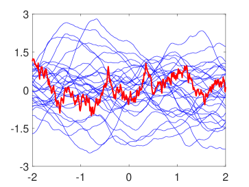
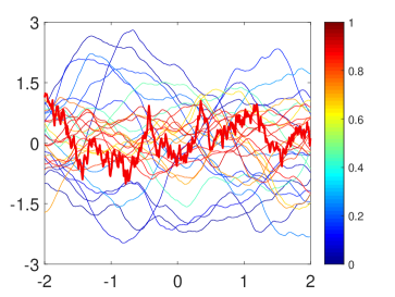
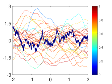
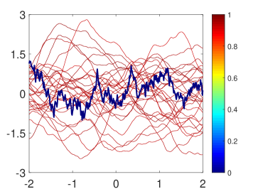
Figure 2: Simulation 1: (a) 30 observed functions, where the red one is generated from GP(0,K1)𝐺𝑃0subscript𝐾1GP(0,K_{1}) and 29 blues ones are generated from GP(0,K2)𝐺𝑃0subscript𝐾2GP(0,K_{2}). (b) The 30 functions with color-labeled depth using 𝕃2superscript𝕃2\mathbb{L}^{2} norm. Observations assigned with color closer to red are considered to be deeper than those assigned with color closer to blue. (c),(d) Same as (b) except for 𝕃2superscript𝕃2\mathbb{L}^{2} norm on the first and second-order derivative functions, respectively.

For better visualization, we sample only one function from GP(0,K1)𝐺𝑃0subscript𝐾1GP(0,K_{1}) on [0,1]01[0,1], and then mix it with another n=29𝑛29n=29 simulated samples from GP(0,K2)𝐺𝑃0subscript𝐾2GP(0,K_{2}) on [0,1]01[0,1]. All these 30 functions are shown in Figure 2(a). It is apparent that the one function from K1subscript𝐾1K_{1} is near the zero-line, but somewhat “noisy”. In contrast, the 29 functions from K2subscript𝐾2K_{2} have high variability in the amplitude, but are very smooth. We then color-labeled them differently in Panels (b)-(d) using their depth values with respect to different criterion functions, namely, 𝕃2superscript𝕃2\mathbb{L}^{2} norm on each function, 𝕃2superscript𝕃2\mathbb{L}^{2} norm on the first-order derivative function, and 𝕃2superscript𝕃2\mathbb{L}^{2} norm on the second-order derivative function. The results clearly illustrate that criteria properly characterize the desirable features in the data. In Panel (b), we rank the function with respect to their 𝕃2superscript𝕃2\mathbb{L}^{2} norm. The one function from K1subscript𝐾1K_{1} is near the zero-line and has the highest depth value. In contrast, since this function is not smooth, it has the least depth values with derivative-based norms in Panels (c) and (d).

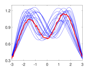
Simulation 2. In this example, we illustrate the time warping distance in the depth computation. We study a set of simulated functions {f1,,f21}subscript𝑓1subscript𝑓21\{f_{1},\cdots,f_{21}\} on [3,3]33[-3,3]. For i=1,,21𝑖121i=1,\cdots,21, we first simulate a set of functions by hi(t)=ϕi,1e(t1.5)2/2+ϕi,2e(t+1.5)2/2subscript𝑖𝑡subscriptitalic-ϕ𝑖1superscript𝑒superscript𝑡1.522subscriptitalic-ϕ𝑖2superscript𝑒superscript𝑡1.522h_{i}(t)=\phi_{i,1}e^{-(t-1.5)^{2}/2}+\phi_{i,2}e^{-(t+1.5)^{2}/2}, where ϕi,1subscriptitalic-ϕ𝑖1\phi_{i,1} and ϕi,2subscriptitalic-ϕ𝑖2\phi_{i,2} are i.i.d. normal with mean one and variance 1/161161/16. Let the warping function γi(t)=6(eai(t+3)/61eai1)3subscript𝛾𝑖𝑡6superscript𝑒subscript𝑎𝑖𝑡361superscript𝑒subscript𝑎𝑖13\gamma_{i}(t)=6(\frac{e^{a_{i}(t+3)/6}-1}{e^{a_{i}}-1})-3 if ai0subscript𝑎𝑖0a_{i}\neq 0 otherwise γi=γidsubscript𝛾𝑖subscript𝛾𝑖𝑑\gamma_{i}=\gamma_{id}, where aisubscript𝑎𝑖a_{i} are equally spaced between 11-1 and 111. The observations are fi(t)=hi(γi(t))subscript𝑓𝑖𝑡subscript𝑖subscript𝛾𝑖𝑡f_{i}(t)=h_{i}(\gamma_{i}(t)) on [3,3],i=1,,21formulae-sequence33𝑖121[-3,3],i=1,\cdots,21. At the final step, we add some noise to the original f11subscript𝑓11f_{11} by f~11(t)=f11(t)+ϵ(t)subscript~𝑓11𝑡subscript𝑓11𝑡italic-ϵ𝑡\tilde{f}_{11}(t)=f_{11}(t)+\epsilon(t), where ϵ(t)italic-ϵ𝑡\epsilon(t) is a Gaussian process with mean 0 and covariance function C(s,t)=0.01δs,t𝐶𝑠𝑡0.01subscript𝛿𝑠𝑡C(s,t)=0.01\delta_{s,t}. To simplify the notation, we abuse f11subscript𝑓11f_{11} to denote the noise contaminated f~11subscript~𝑓11\tilde{f}_{11}.

All these 21 functions are shown in Figure 3(a), where we use red line to represent f11subscript𝑓11f_{11} and blue lines to represent the others. Before computing depth values, we conduct the Fisher-Rao alignment procedure to align the observed functions and obtain the corresponding time warping functions {γ^1(t),,γ^21(t)}subscript^𝛾1𝑡subscript^𝛾21𝑡\{\hat{\gamma}_{1}(t),\cdots,\hat{\gamma}_{21}(t)\} (Srivastava et al., 2011). Let fcsubscript𝑓𝑐f_{c} denote the Karcher mean of {f1,,f21}subscript𝑓1subscript𝑓21\{f_{1},\cdots,f_{21}\} (in the sense of SRVF space). Then the optimal time warping function from fisubscript𝑓𝑖f_{i} to fcsubscript𝑓𝑐f_{c} is γ^i,i=1,,21formulae-sequencesubscript^𝛾𝑖𝑖121\hat{\gamma}_{i},i=1,\cdots,21.

Refer to caption
(a) Observed functions
Refer to caption
(b) ζ(fi,fc)=γ^iγid2𝜁subscript𝑓𝑖subscript𝑓𝑐subscriptnormsubscript^𝛾𝑖subscript𝛾𝑖𝑑2\zeta(f_{i},f_{c})=\|\hat{\gamma}_{i}-\gamma_{id}\|_{2}
Refer to caption
(c) ζ(fi,fc)=dFR(γ^i,γid)𝜁subscript𝑓𝑖subscript𝑓𝑐subscript𝑑𝐹𝑅subscript^𝛾𝑖subscript𝛾𝑖𝑑\zeta(f_{i},f_{c})=d_{FR}(\hat{\gamma}_{i},\gamma_{id})
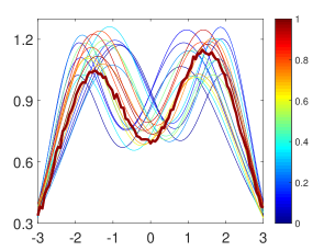
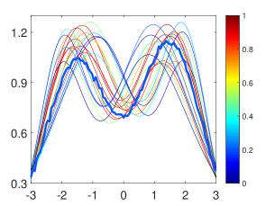
Figure 3: Simulation 2: (a) 21 observed functions, where f11subscript𝑓11f_{11} is emphasized in red color. (b) The 21 functions with color-labeled depth via the 𝕃2superscript𝕃2\mathbb{L}^{2} warping distance γ^iγid2subscriptnormsubscript^𝛾𝑖subscript𝛾𝑖𝑑2\|\hat{\gamma}_{i}-\gamma_{id}\|_{2}. (c) Same as (b) except for the Fisher-Rao distance dFR(γ^i,γid)subscript𝑑𝐹𝑅subscript^𝛾𝑖subscript𝛾𝑖𝑑d_{FR}(\hat{\gamma}_{i},\gamma_{id}).

We take the criterion function ζ(fi,fc)=γ^iγid2𝜁subscript𝑓𝑖subscript𝑓𝑐subscriptnormsubscript^𝛾𝑖subscript𝛾𝑖𝑑2\zeta(f_{i},f_{c})=\|\hat{\gamma}_{i}-\gamma_{id}\|_{2} for the depth computation. The 21 color-labeled functions using depth values are shown in Figure 3(b). In general, functions in the middle along x-axis have large depth values, whereas those at each side have low values. In particular, because f11subscript𝑓11f_{11} stays in the middle of the observations, it has the least 𝕃2superscript𝕃2\mathbb{L}^{2} warping distance from fcsubscript𝑓𝑐f_{c} and largest depth values. As comparison we also use the well-known Fisher-Rao distance function ζ(fi,fc)=dFR(γ^i,γid)𝜁subscript𝑓𝑖subscript𝑓𝑐subscript𝑑𝐹𝑅subscript^𝛾𝑖subscript𝛾𝑖𝑑\zeta(f_{i},f_{c})=d_{FR}(\hat{\gamma}_{i},\gamma_{id}) for the depth computation. The 21 color-labeled functions using depth values are shown in Figure 3(c). As the Fisher-Rao distance is derivative-based, small perturbation on time warping results in large difference. The small noise on f11subscript𝑓11f_{11} makes it have smallest depth value in the 21 functions. For other 20 smooth functions, their depth values are consistent to those in Panel (b).

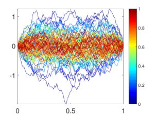
Simulation 3. In this illustration, we demonstrate Algorithm I in Section 3 for modified norm-based depth estimation on a variant of the continuous-time Brownian Bridge on [0,1]01[0,1], with different choices of decaying weight sequences {ap}subscript𝑎𝑝\{a_{p}\}, where the covariance kernel function is K(s,t)=min(s,t)st𝐾𝑠𝑡𝑚𝑖𝑛𝑠𝑡𝑠𝑡K(s,t)=min(s,t)-st for any s,t[0,1]𝑠𝑡01s,t\in[0,1]. According to the notation in Equations (1) and (2), we have λp=1p2π2,ϕp(t)=2sin(πpt)formulae-sequencesubscript𝜆𝑝1superscript𝑝2superscript𝜋2subscriptitalic-ϕ𝑝𝑡2𝑠𝑖𝑛𝜋𝑝𝑡\lambda_{p}=\frac{1}{p^{2}\pi^{2}},\phi_{p}(t)=\sqrt{2}sin(\pi pt), and can simulate fpsubscript𝑓𝑝f_{p} from independent Laplace distribution with mean 0 and variance λpsubscript𝜆𝑝\lambda_{p} for p=1,2,𝑝12p=1,2,\cdots (note that this is different from the normal distribution 𝒩(0,λp)𝒩0subscript𝜆𝑝\mathcal{N}(0,\lambda_{p}) in a Brownian bridge).

More specifically, we sample {fi(t)}subscript𝑓𝑖𝑡\{f_{i}(t)\} by the linear combination fi(t)=p=11000fi,pϕp(t),i=1,,n(=100)formulae-sequencesubscript𝑓𝑖𝑡superscriptsubscript𝑝11000subscript𝑓𝑖𝑝subscriptitalic-ϕ𝑝𝑡𝑖1annotated𝑛absent100f_{i}(t)=\sum_{p=1}^{1000}f_{i,p}\phi_{p}(t),i=1,\cdots,n(=100) to approximate the infinite-dimensional stochastic process. We set N=1000𝑁1000N=1000 in the Monte Carlo sampling. We have three different settings to choose the weight coefficients {ap}subscript𝑎𝑝\{a_{p}\}: a)ap1,b)ap=1/p,a)\ a_{p}\equiv 1,\ b)\ a_{p}=1/p, and c)ap=1/[plog(p+1)],p=1,,Nc)\ a_{p}=1/[\sqrt{p}\log(p+1)],p=1,\cdots,N. In Case a), there is actually no weight terms, and the modified norm is equal to the RKHS induced norm. In Figure 4(a), we show the 100 functions with color-labeled using its depth value from this norm. Note that we compute this norm in a finite-dimensional setup and it will diverge to \infty when N𝑁N is large. It is straightforward to find that

fi𝕃22=p=1N012π2p2fi,p2cos(πpt)2𝑑t=p=1Nπ2p2fi,p2=p=1Nfi,p2λp=fiK2.superscriptsubscriptnormsuperscriptsubscript𝑓𝑖superscript𝕃22superscriptsubscript𝑝1𝑁superscriptsubscript012superscript𝜋2superscript𝑝2superscriptsubscript𝑓𝑖𝑝2𝑐𝑜𝑠superscript𝜋𝑝𝑡2differential-d𝑡superscriptsubscript𝑝1𝑁superscript𝜋2superscript𝑝2superscriptsubscript𝑓𝑖𝑝2superscriptsubscript𝑝1𝑁superscriptsubscript𝑓𝑖𝑝2subscript𝜆𝑝superscriptsubscriptnormsubscript𝑓𝑖subscript𝐾2\|f_{i}^{{}^{\prime}}\|_{\mathbb{L}^{2}}^{2}=\sum_{p=1}^{N}\int_{0}^{1}2\pi^{2}p^{2}\cdot f_{i,p}^{2}cos(\pi pt)^{2}dt=\sum_{p=1}^{N}\pi^{2}p^{2}f_{i,p}^{2}=\sum_{p=1}^{N}\frac{f_{i,p}^{2}}{\lambda_{p}}=\|f_{i}\|_{\mathbb{H}_{K}}^{2}. (10)

That is, the RKHS induced norm is the same as 𝕃2superscript𝕃2\mathbb{L}^{2} norm on the derivative function, a common measure of smoothness of a function.

In Cases b) and c), the series satisfies the convergent requirement limNi=1NaP2<subscript𝑁superscriptsubscript𝑖1𝑁superscriptsubscript𝑎𝑃2\lim_{N\rightarrow\infty}\sum_{i=1}^{N}a_{P}^{2}<\infty, and therefore the modified norms are well-defined. In particular, we find that when ap=1/psubscript𝑎𝑝1𝑝a_{p}=1/p, the classical 𝕃2superscript𝕃2\mathbb{L}^{2} norm

fi𝕃22=p=1N01fi,p2ϕp2(t)𝑑t=p=1Nfi,p2=1π2p=1Nfi,p211/π2p21p2fimod2.superscriptsubscriptnormsubscript𝑓𝑖superscript𝕃22superscriptsubscript𝑝1𝑁superscriptsubscript01superscriptsubscript𝑓𝑖𝑝2superscriptsubscriptitalic-ϕ𝑝2𝑡differential-d𝑡superscriptsubscript𝑝1𝑁superscriptsubscript𝑓𝑖𝑝21superscript𝜋2superscriptsubscript𝑝1𝑁superscriptsubscript𝑓𝑖𝑝211superscript𝜋2superscript𝑝21superscript𝑝2proportional-tosuperscriptsubscriptnormsubscript𝑓𝑖𝑚𝑜𝑑2\|f_{i}\|_{\mathbb{L}^{2}}^{2}=\sum_{p=1}^{N}\int_{0}^{1}f_{i,p}^{2}\phi_{p}^{2}(t)dt=\sum_{p=1}^{N}f_{i,p}^{2}=\frac{1}{\pi^{2}}\sum_{p=1}^{N}f_{i,p}^{2}\cdot\frac{1}{1/\pi^{2}p^{2}}\cdot\frac{1}{p^{2}}\propto\|f_{i}\|_{mod}^{2}. (11)

That is, the modified norm in Case b) is proportional to the 𝕃2superscript𝕃2\mathbb{L}^{2} norm. This explains the result in Figure 4(b) where the 100 functions are color-labeled using its depth value from this norm. We can see that high-depth functions are near the zero-line and low-depth functions are near boundary lines. This depth reflects the traditional functional depths such as band depth and half-region depth (López-Pintado & Romo, 2009, 2011). In Case c), we use another type of weight coefficient and the depth result is shown in Figure 4(c), which is very similar to the result in Case b). In summary, we have found that 1) the modified norms can provide different forms of measurement on the center-out rank on the given functional observation and some of the special forms are consistent to the classical norms; and 2) the rank may be robust with respect to different choices of norm.
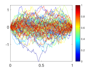
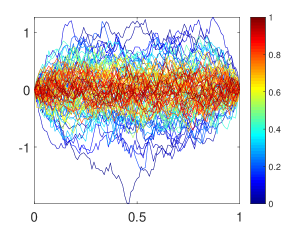
Refer to caption
(a) ap=1subscript𝑎𝑝1a_{p}=1
Refer to caption
(b) ap=1/psubscript𝑎𝑝1𝑝a_{p}=1/p
Refer to caption
(c) ap=1/[plog(p+1)]subscript𝑎𝑝1delimited-[]𝑝𝑝1a_{p}=1/[\sqrt{p}\log(p+1)]
Figure 4: Simulated functions with color-labeled depth. (a) Each function is color-labeled using its depth value, where the sequence {ap}subscript𝑎𝑝\{a_{p}\} is constant 1. Observations assigned with color closer to red are considered to be deeper than those assigned with color closer to blue. (b) and (c), Same as (a) except that the coefficients ap=1/psubscript𝑎𝑝1𝑝a_{p}=1/p and ap=1/1/[plog(p+1)],p=1,,Nformulae-sequencesubscript𝑎𝑝11delimited-[]𝑝𝑝1𝑝1𝑁a_{p}=1/1/[\sqrt{p}\log(p+1)],p=1,\cdots,N, respectively.

Simulation 4. We consider a finite-dimensional Gaussian process by selecting a sequence of orthonormal Fourier basis functions up to order P=10𝑃10P=10 on [0,1]01[0,1] such that

ϕp(t)={1p=12cos(πpt)p=2,4,6,8,102sin(π(p1)t)p=3,5,7,9,subscriptitalic-ϕ𝑝𝑡cases1missing-subexpression𝑝12𝜋𝑝𝑡missing-subexpression𝑝2468102𝜋𝑝1𝑡missing-subexpression𝑝3579\displaystyle\phi_{p}(t)=\left\{\begin{array}[]{ccl}1&&p=1\\ \sqrt{2}\cos(\pi pt)&&p=2,4,6,8,10\\ \sqrt{2}\sin(\pi(p-1)t)&&p=3,5,7,9\end{array}\right.,

and a set of coefficients {a1,,aP}N(0,I10)similar-tosubscript𝑎1subscript𝑎𝑃𝑁0subscript𝐼10\{a_{1},\cdots,a_{P}\}\sim N(0,I_{10}). Then we generate N=500𝑁500N=500 functions via linear combination fi=p=1Pai,pϕpsubscript𝑓𝑖superscriptsubscript𝑝1𝑃subscript𝑎𝑖𝑝subscriptitalic-ϕ𝑝f_{i}=\sum_{p=1}^{P}a_{i,p}\phi_{p}. Panel (a) in Figure 5 shows n=21𝑛21n=21 randomly selected samples from {fi(t),t[0,1]}i=1Nsuperscriptsubscriptsubscript𝑓𝑖𝑡𝑡01𝑖1𝑁\{f_{i}(t),t\in[0,1]\}_{i=1}^{N}.

Refer to caption
(a) 21 functions from the original sample
Refer to caption
(b) Estimated eigenvalues
Refer to caption
(c) Histogram of squared RKHS norm
Refer to caption
(d) Samples with color-labeled depth
Figure 5: Finite Gaussian Process Illustration: (a) 21 randomly selected samples; (b) Estimated eigenvalues λ^psubscript^𝜆𝑝\hat{\lambda}_{p} from the covariance K^^𝐾\hat{K}; (c) Histogram of squared RKHS norm fiK^2=p=110a^i,p2λ^p,nsuperscriptsubscriptnormsubscript𝑓𝑖subscript^𝐾2superscriptsubscript𝑝110superscriptsubscript^𝑎𝑖𝑝2subscript^𝜆𝑝𝑛\|f_{i}\|_{\mathbb{H}_{\hat{K}}}^{2}=\sum_{p=1}^{10}\frac{\hat{a}_{i,p}^{2}}{\hat{\lambda}_{p,n}}, where the red line indicates a fit to chi-square distribution χ2(10)superscript𝜒210\chi^{2}(10); (d) Estimated depth of the 21 samples with color-label, where blue to red indicates the depth value range of [0,1]01[0,1].

From Panel (b) in Figure 5, it is clear that there exists a significant gap in the decreasing sequence of estimated eigenvalues, and the gap locates just after the order of the dimension P=10𝑃10P=10. This indicates the correct dimension can be easily estimated. From Panel (c), we can tell that the squared RKHS norm fits χ2(P)superscript𝜒2𝑃\chi^{2}(P) well. This is also consistent to the above theoretical derivation. The estimated depth values are color-labeled in Panel (d). We note that the RKHS induced norm does not have a conventional 𝕃2superscript𝕃2\mathbb{L}^{2} type of norm, so there is no direct visualization to evaluate the depth in this example. However, we point out that if the data are generated from two random processes, these depth values can help differentiate the observations, as illustrated in the following.

In particular, we show how the model-based depth can be used for the classification purpose, and compare the performance between RKHS norm and the modified one. Specifically, we select a sequence of orthonormal Fourier basis functions up to order P𝑃P on [0,1]01[0,1] such that for p=1,2,,P𝑝12𝑃p=1,2,\cdots,P,

ϕp(t)={2sin(π(p+1)pt)p is odd2cos(πpt)p is even,subscriptitalic-ϕ𝑝𝑡cases2𝜋𝑝1𝑝𝑡missing-subexpression𝑝 is odd2𝜋𝑝𝑡missing-subexpression𝑝 is even\displaystyle\phi_{p}(t)=\left\{\begin{array}[]{ccl}\sqrt{2}\sin(\pi(p+1)pt)&&p\mbox{ is odd}\\ \sqrt{2}\cos(\pi pt)&&p\mbox{ is even}\end{array}\right.,

Then we generate 454545 functions as fi(t)=p=1Pai,pϕp(t),i=1,,45formulae-sequencesubscript𝑓𝑖𝑡superscriptsubscript𝑝1𝑃subscript𝑎𝑖𝑝subscriptitalic-ϕ𝑝𝑡𝑖145f_{i}(t)=\sum_{p=1}^{P}a_{i,p}\phi_{p}(t),i=1,\cdots,45 and 555 functions as fi(t)=p=1Pbi,pϕp(t),i=46,,50formulae-sequencesubscript𝑓𝑖𝑡superscriptsubscript𝑝1𝑃subscript𝑏𝑖𝑝subscriptitalic-ϕ𝑝𝑡𝑖4650f_{i}(t)=\sum_{p=1}^{P}b_{i,p}\phi_{p}(t),i=46,\cdots,50, where independent coefficients ai,pN(0,1)similar-tosubscript𝑎𝑖𝑝𝑁01a_{i,p}\sim N(0,1) and bi,pN(0,3)similar-tosubscript𝑏𝑖𝑝𝑁03b_{i,p}\sim N(0,3). Due to the different variance values on the coefficients, the first 45 functions are in the main cluster and the last 5 functions are outliers. One special case when only P=4𝑃4P=4 low frequency basis functions are used is shown in Figure 6(a). Because of the smaller coefficient variance, the first 45 functions are in a main cluster. In contrast, some of the last 5 function have much larger amplitude and are apparently outliers. In another example, we use P=100𝑃100P=100 basis functions shown in Figure 6(b). As compared to when P=4𝑃4P=4, both main clusters functions and the 5 outliers have much higher frequency components.
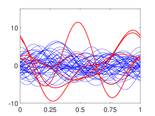
Refer to caption
(a) 50 functions with P=4𝑃4P=4
Refer to caption
(b) 50 functions with P=100𝑃100P=100
Refer to caption
(c) Depths with P=4𝑃4P=4
Refer to caption
(d) Depths with P=100𝑃100P=100
Refer to caption
(e) Overall accuracy rate
Refer to caption
(f) Outlier detection rate
Figure 6: Classification by depth values: (a) 50 function samples for P=4𝑃4P=4, where the blue ones represent 45 functions in the main cluster and the red ones represent 5 outliers. (b) Same as (a) except P=100𝑃100P=100. (c) Depth values of the 50 functions with P=4𝑃4P=4 using the RKHS norm (green circles over blue lines) and modified RKHS norm (yellow squares over red lines). (d) Same as (c) except P=100𝑃100P=100. (e) The classification accuracy for all 50 functions by using the RKHS norm (blue line) and modified RKHS norm (red line), where P𝑃P varies on seven different values 4, 10, 20, 30, 40, 70, and 100. (f) Same as (e) except the accuracy on the 5 outlier functions.

We have shown that the RKHS induced norm can characterize the smoothness level in Equation (10) and the modified RKHS norm can characterize the amplitude level (𝕃2superscript𝕃2\mathbb{L}^{2} norm) in Equation (11). We at first use these two norms for the case when P=4𝑃4P=4 and the result on depth values are shown in Figure 6(c). Note that for the simulated 5 outliers, only 3 of them show large amplitude as compared to the main cluster, and therefore only these three have relatively lower depth values by using either RKHS norm or the modified norm. In contrast, when P=100𝑃100P=100, the difference on amplitude for the main cluster and the 5 outliers are apparent. This can be easily seen using the modified norm shown in Figure 6(d). As all high frequency basis functions can have large un-smooth level, the RKHS norm is not able to clearly differentiate 5 outliers from the main cluster. This is also shown in Figure 6(d).

To measure the classification performance, we set a threshold of 0.1 on the depth value for all functions. This is done for the number of basis components P𝑃P being 4, 10, 20, 30, 40, 70, or 100, which varies from highly smooth to highly nonsmooth observations. The classification result on all 50 functions is shown in Figure 6(e). In particular, we also show the detection on the 5 outliers in Figure 6(f). When P𝑃P is small, both norms produce reasonable classification accuracy around 95% (a couple of errors in the outliers). When P𝑃P gets larger, the modified RKHS can capture larger amplitude in the outliers and reach 100% classification accuracy. In contrast, all 50 functions have similar smoothing level which makes the RKHS norm not able to detect the outliers.

5.2 Real Data Illustration
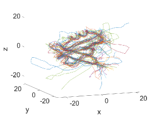
Refer to caption
(a) 3-D data
Refer to caption
(b) Component-wise data
Refer to caption
(c) Depth with ζ(f)=f2𝜁𝑓subscriptnorm𝑓2\zeta(f)=\|f\|_{2}
Refer to caption
(d) Depth with ζ(f)=f2𝜁𝑓subscriptnormsuperscript𝑓2\zeta(f)=\|f^{\prime}\|_{2}
Refer to caption
(e) Outliers in 3-D
Refer to caption
(f) Outlier components
Figure 7: Real data example: (a) 3-dimensional data of 23 PDZ domain observations. (b) The 3-coordinate components of given observations. (c) Depth values computed using the classical 𝕃2superscript𝕃2\mathbb{L}^{2} norm. (d) Depth values computed using the 𝕃2superscript𝕃2\mathbb{L}^{2} norm on the first derivative functions. (e) Detected outliers (black dash lines) in 3-dimension by using depth values. (f) 3-coordinate components of the detected outliers (black dashed lines).

In this subsection, we apply our proposed method to detect outliers on a real dataset. The dataset is taken from the SCOP database (Murzin et al., 1995). We take the subset of proteins with sample size 23 from PDZ domain using PISCES server (Wang & Dunbrack Jr, 2003). The data have been pre-processed as described in (Wu et al., 2013), and we get normalized data where the three componenets are properly rotated and aligned. This given data are shown in Figure 7(a) as 3-dimensional curves and the three coponents are shown in Figure 7(b).

This given data has been applied with two different norms; one is the classical 𝕃2superscript𝕃2\mathbb{L}^{2} norm on 3-dimensional functions and the other is the 𝕃2superscript𝕃2\mathbb{L}^{2} norm on the first derivative functions. The depth values computed by these two different norms are shown in Fig 7(c) and (d), respectively. We note that the depth results are vey close to each for the two norms – both methods indicate that the 8th and 12th protein sequences are outliers in our dataset by using a detection threshold α=0.05𝛼0.05\alpha=0.05. The two outliers are shown in Figure 7(e) and (f) as 3-dimensional curves and for 3 coordinate components, respectively. It is apparent that the depth values successfully detect the outliers in the given data.
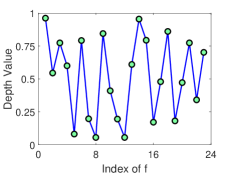
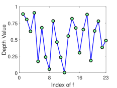
Refer to caption
(a) RKHS norm
Refer to caption
(b) Modified RKHS
Refer to caption
(c) Band depth
Refer to caption
(d) Modified band depth
Figure 8: Comparison: (a) Depth values using RKHS induced norm. (b) Depth values using modified RKHS norm with ap=1/psubscript𝑎𝑝1𝑝a_{p}=1/p. (c) Depth values computed using band depth method. (d) Depth values computed using modified band depth method.

For comparison, the depth values obtained by the RKHS norm in our framework are shown in Figure 8(a), where a lot of functions have low depth values and the two outliers cannot be clearly identified. Figure 8(b) shows the depth values computed by modified norm with ap=1/psubscript𝑎𝑝1𝑝a_{p}=1/p in our model based depth framework. It is clearly to see that the 8th and 12th functions have lowest depth values, though not as close to 0 as the two 𝕃2superscript𝕃2\mathbb{L}^{2} norms in Figure 7.

In addition, we compare our approach to the well-known depth methods – band depth and its modified version (López-Pintado & Romo, 2009). The performance of band depth shown in Figure 8(c) is very poor, and it implies that there are great difficulties in applying the band depth due to large variation in the three coordinates. On the other hand, the result in Figure 8(d) shows that depth values obtained by modified band depth have a clear large gap between the two outliers and main portion of the data, consistent to the result in Figure 7, whereas the depth values are distributed in a very narrow range.

6 Summary and Future works

In this article, we have proposed a new framework to define model-based statistical depth for functional as well as multivariate observations. Our definitions have two forms: norm-based and inner-product-based. Depending on the selection (of norms), the norm-based depth can have various center-outward ranks. For the inner-product depth, it is mainly the generalization of the multivariate halfspace depth. We then focus on using norms which are naturally defined with the generative model. That is, we use induced RKHS norm from the finite-dimensional covariance kernel in a second-ordered stochastic process. For an infinite-dimensional kernel, we have introduced a modified version to avoid the infinity value on the induced norm. For practical use, we propose efficient algorithms to compute the proposed depths. Through simulations and real data, we demonstrate the proposed depths reveal important statistical properties of given observations, such as median and quantiles. Furthermore, we establish the consistency theory on the estimators.

Statistical depth is an extensively-studied area. However, all previous methods are either procedure-based or properties-based. To the best of our knowledge, this is the first model-based investigation. This paper introduced the basic framework, but the model is limited to covariance-based method. Due to the nature of covariance kernel, our framework have a tendency to deal with second-order stochastic process like Gaussian family well. We plan to work in a space where higher order statistics can also be important in the future. In addition, we have discussed four important properties for the proposed depths. As Gijbels et al. (2017) provided an elaboration on more desirable properties (such as receptivity and continuity) of statistical depths for functional data, our future work is to investigate whether our proposed framework would meet those properties. Moveover, since we obtain median and quantiles by the proposed depths, we can also extend our method to construct boxplot visualization. Last but not least, we are seeking broader applications of the new framework in real world problems such as clustering, classification, and outlier detection.


Supplement to Model-based Statistical Depth with Applications to Functional Data

Appendix A Algorithms for general model-based depth

Suppose we have n𝑛n zero-mean independent sample functions f1,,fnsubscript𝑓1subscript𝑓𝑛f_{1},\cdots,f_{n}\in\mathcal{F} on t[0,1]𝑡01t\in[0,1], and our goal is to compute the model-based depth of any observed sample fobssubscript𝑓𝑜𝑏𝑠f_{obs}\in\mathcal{F}. We first describe the norm-based depth estimation algorithm as follows:

Algorithm II. (Input: observations {f1,,fn}subscript𝑓1subscript𝑓𝑛\{f_{1},\cdots,f_{n}\}, any observation fobssubscript𝑓𝑜𝑏𝑠f_{obs}, a threshold ϵ>0italic-ϵ0\epsilon>0, the center function fcsubscript𝑓𝑐f_{c}, and the selected norm \|\cdot\|, which means ζ(f,fc)=ffc𝜁𝑓subscript𝑓𝑐norm𝑓subscript𝑓𝑐\zeta(f,f_{c})=\|f-f_{c}\| for any observation f𝑓f.)

  1. 1.

    Compute the sample mean function f¯(t)=1ni=1nfi(t)¯𝑓𝑡1𝑛superscriptsubscript𝑖1𝑛subscript𝑓𝑖𝑡\bar{f}(t)=\frac{1}{n}\sum_{i=1}^{n}f_{i}(t), and empirical covariance kernel K^(s,t)=1ni=1n[fi(s)f¯(s)][fi(t)f¯(t)]^𝐾𝑠𝑡1𝑛superscriptsubscript𝑖1𝑛delimited-[]subscript𝑓𝑖𝑠¯𝑓𝑠delimited-[]subscript𝑓𝑖𝑡¯𝑓𝑡\hat{K}(s,t)=\frac{1}{n}\sum_{i=1}^{n}[f_{i}(s)-\bar{f}(s)][f_{i}(t)-\bar{f}(t)];

  2. 2.

    Eigen-decompose K^=p=1nλ^p,nϕ^p,n(s)ϕ^p,n(t)^𝐾superscriptsubscript𝑝1𝑛subscript^𝜆𝑝𝑛subscript^italic-ϕ𝑝𝑛𝑠subscript^italic-ϕ𝑝𝑛𝑡\hat{K}=\sum_{p=1}^{n}\hat{\lambda}_{p,n}\hat{\phi}_{p,n}(s)\hat{\phi}_{p,n}(t);

  3. 3.

    Choose a number P𝑃P if λ^P+1subscript^𝜆𝑃1\hat{\lambda}_{P+1} is the first eigenvalue such that λ^P+1<ϵsubscript^𝜆𝑃1italic-ϵ\hat{\lambda}_{P+1}<\epsilon for sufficiently small ϵitalic-ϵ\epsilon; then K^(s,t)=p=1Pλ^p,nϕ^p,n(s)ϕ^p,n(t)^𝐾𝑠𝑡superscriptsubscript𝑝1𝑃subscript^𝜆𝑝𝑛subscript^italic-ϕ𝑝𝑛𝑠subscript^italic-ϕ𝑝𝑛𝑡\hat{K}(s,t)=\sum_{p=1}^{P}\hat{\lambda}_{p,n}\hat{\phi}_{p,n}(s)\hat{\phi}_{p,n}(t);

  4. 4.

    Compute f^i,p=01fi(t)ϕ^p,n(t)𝑑tsubscript^𝑓𝑖𝑝superscriptsubscript01subscript𝑓𝑖𝑡subscript^italic-ϕ𝑝𝑛𝑡differential-d𝑡\hat{f}_{i,p}=\int_{0}^{1}f_{i}(t)\hat{\phi}_{p,n}(t)dt for all i=1,,n𝑖1𝑛i=1,\cdots,n and p=1,,P𝑝1𝑃p=1,\cdots,P, and compute f^p=01fobs(t)ϕ^p,n(t)𝑑tsubscript^𝑓𝑝superscriptsubscript01subscript𝑓𝑜𝑏𝑠𝑡subscript^italic-ϕ𝑝𝑛𝑡differential-d𝑡\hat{f}_{p}=\int_{0}^{1}f_{obs}(t)\hat{\phi}_{p,n}(t)dt;

  5. 5.

    Re-sample (with replacement) a large number N𝑁N of coefficients {g^j,p}j=1Nsuperscriptsubscriptsubscript^𝑔𝑗𝑝𝑗1𝑁\{\hat{g}_{j,p}\}_{j=1}^{N} based on the coefficients of {f^i,p}subscript^𝑓𝑖𝑝\{\hat{f}_{i,p}\}, and construct gj(t)=p=1Pg^j,pϕp^(t)subscript𝑔𝑗𝑡superscriptsubscript𝑝1𝑃subscript^𝑔𝑗𝑝^subscriptitalic-ϕ𝑝𝑡g_{j}(t)=\sum_{p=1}^{P}\hat{g}_{j,p}\hat{\phi_{p}}(t);

  6. 6.

    Estimate the sample depth of fobssubscript𝑓𝑜𝑏𝑠f_{obs} w.r.t. {gj}subscript𝑔𝑗\{g_{j}\}:

    Dn(fobs;{gj}j=1N)=1Nj=1N1(ζ(fobs,fc)ζ(gj,fc))=1Nj=1N1(fobsfcgjfc),subscript𝐷𝑛subscript𝑓𝑜𝑏𝑠superscriptsubscriptsubscript𝑔𝑗𝑗1𝑁1𝑁superscriptsubscript𝑗1𝑁subscript1𝜁subscript𝑓𝑜𝑏𝑠subscript𝑓𝑐𝜁subscript𝑔𝑗subscript𝑓𝑐1𝑁superscriptsubscript𝑗1𝑁subscript1normsubscript𝑓𝑜𝑏𝑠subscript𝑓𝑐normsubscript𝑔𝑗subscript𝑓𝑐\displaystyle D_{n}(f_{obs};\{g_{j}\}_{j=1}^{N})=\frac{1}{N}\sum_{j=1}^{N}\textbf{1}_{(\zeta(f_{obs},f_{c})\leq\zeta(g_{j},f_{c}))}=\frac{1}{N}\sum_{j=1}^{N}\textbf{1}_{(\|f_{obs}-f_{c}\|\leq\|g_{j}-f_{c}\|)},

    where 1()subscript1\textbf{1}_{(\cdot)} is the indicator function.

Steps 1-4 are the first part in the algorithm. They aim to estimate the eigen-system of the covariance kernel via given observations. In particular, the Karhunen Loève expansion (Ash, 1990) is used in Step 2 to decompose the covariance kernel, and offer a method to reconstruct samples (the background on the Karhunen Loève expansion will be provided in Section 3). Using a functional principal component analysis (Ramsay, 2005), we retain the eigen-functions which explain meaningful variance in our system. Steps 5-6 are the second part of the algorithm. They estimate the depth value with the given norm, where we need re-sampling techniques and Monte Carlo approximations. This algorithm can be easily adapted to the multivariate data. In such case, the dimension of the data is already given and the principal component analysis and the multivariate metric can be directly applied.

In general, computing a halfspace depth in dsuperscript𝑑\mathbb{R}^{d} is a very challenging task. So far, exact computations can be given only when d=2𝑑2d=2 (Rousseeuw & Ruts, 1996) and d=3𝑑3d=3 (Rousseeuw & Struyf, 1998). There are approximation algorithms when d4𝑑4d\geq 4 (Zuo, 2018). However, if the data distribution is a multivariate normal, our framework will result in an optimal solution similar to that obtained for the Gaussian process. For infinite dimensional GP, Lemma 1 shows that the inner-produt-based depth can only be feasible for finite-dimensional space. Fortunately, when the random samples are from a finite-dimensional zero-mean Gaussian process, the depth has simple closed-form (see detail in Appendix A). We adopt this special case and modify the above algorithm for halfspace depth as follows, where Steps 4-6 are simplified as follows:

  1. 4.

    Compute f^p=01fobs(t)ϕ^p,n(t)𝑑tsubscript^𝑓𝑝superscriptsubscript01subscript𝑓𝑜𝑏𝑠𝑡subscript^italic-ϕ𝑝𝑛𝑡differential-d𝑡\hat{f}_{p}=\int_{0}^{1}f_{obs}(t)\hat{\phi}_{p,n}(t)dt for p=1,,P𝑝1𝑃p=1,\cdots,P;

  2. 5.

    Compute the induced RKHS norm fobsK^2=p=1Pf^p2λ^p,nsuperscriptsubscriptnormsubscript𝑓𝑜𝑏𝑠subscript^𝐾2superscriptsubscript𝑝1𝑃superscriptsubscript^𝑓𝑝2subscript^𝜆𝑝𝑛\|f_{obs}\|_{\mathbb{H}_{\hat{K}}}^{2}=\sum_{p=1}^{P}\frac{\hat{f}_{p}^{2}}{\hat{\lambda}_{p,n}};

  3. 6.

    Compute the depth as Dip(fobs)=1Φ(fobsK^)subscript𝐷𝑖𝑝subscript𝑓𝑜𝑏𝑠1Φsubscriptnormsubscript𝑓𝑜𝑏𝑠subscript^𝐾D_{ip}(f_{obs})=1-\Phi(||f_{obs}||_{\mathbb{H}_{\hat{K}}}), where Φ(x)Φ𝑥\Phi(x) denotes the cumulative distribution function of a standard normal random variable.

Appendix B Applications of norm-based depth in finite-dimensional Process

Finite-dimensional process is a commonly used stochastic process in practical applications. In particular, this include any finite-dimensional Gaussian Process (GP) and multivariate Gaussian distribution as special cases. In this appendix, we simplify our model in Section 3.2 into a zero-mean finite-dimensional process, which means that K𝐾K has a finite number P𝑃P of positive eigenvalues, and P𝑃P will be referred as the dimension of this process. That is, K(s,t)=j=1Pλjϕj(s)ϕj(t)𝐾𝑠𝑡superscriptsubscript𝑗1𝑃subscript𝜆𝑗subscriptitalic-ϕ𝑗𝑠subscriptitalic-ϕ𝑗𝑡K(s,t)=\sum_{j=1}^{P}\lambda_{j}\phi_{j}(s)\phi_{j}(t). For convenience we denote this kernel as K=KP𝐾subscript𝐾𝑃K=K_{P}. One important benefit in this process is that the associated RKHS norm is always finite and can be directly used in our construction of norm-induced depth as described in Section 5.1.

B.1 RKHS norm induced depth for finite-dimensional process

Suppose we have functional observation f𝕃2([0,1])𝑓superscript𝕃201f\in\mathbb{L}^{2}([0,1]) from a zero-mean stochastic process with covariance kernel KP(s,t)=p=1Pλpϕp(s)ϕp(t)subscript𝐾𝑃𝑠𝑡superscriptsubscript𝑝1𝑃subscript𝜆𝑝subscriptitalic-ϕ𝑝𝑠subscriptitalic-ϕ𝑝𝑡K_{P}(s,t)=\sum_{p=1}^{P}\lambda_{p}\phi_{p}(s)\phi_{p}(t) on [0,1]×[0,1]0101[0,1]\times[0,1]. Then f(t)=p=1Pfpϕp(t)𝑓𝑡superscriptsubscript𝑝1𝑃subscript𝑓𝑝subscriptitalic-ϕ𝑝𝑡f(t)=\sum_{p=1}^{P}f_{p}\phi_{p}(t), where f1,,fPsubscript𝑓1subscript𝑓𝑃f_{1},\cdots,f_{P} are uncorrelated and E(fp)=0,E(fp2)=λp,j=1,,Pformulae-sequence𝐸subscript𝑓𝑝0formulae-sequence𝐸superscriptsubscript𝑓𝑝2subscript𝜆𝑝𝑗1𝑃E(f_{p})=0,E(f_{p}^{2})=\lambda_{p},j=1,\cdots,P. In particular, when the process is a Gaussian process, f1,,fPsubscript𝑓1subscript𝑓𝑃f_{1},\cdots,f_{P} are independent. In this case, {Xp=fp/λp}p=1Psuperscriptsubscriptsubscript𝑋𝑝subscript𝑓𝑝subscript𝜆𝑝𝑝1𝑃\{X_{p}=f_{p}/\sqrt{\lambda_{p}}\}_{p=1}^{P} are i.i.d. samples from a standard normal distribution, and the squared induced norm fK2=p=1Pfp2/λp=p=1PXp2superscriptsubscriptnorm𝑓subscript𝐾2superscriptsubscript𝑝1𝑃superscriptsubscript𝑓𝑝2subscript𝜆𝑝superscriptsubscript𝑝1𝑃superscriptsubscript𝑋𝑝2\|f\|_{\mathbb{H}_{K}}^{2}=\sum_{p=1}^{P}f_{p}^{2}/\lambda_{p}=\sum_{p=1}^{P}X_{p}^{2} follows a χ2superscript𝜒2\chi^{2} distribution with P𝑃P degrees of freedom, denoted as χ2(P)superscript𝜒2𝑃\chi^{2}(P).

The computation of depth still depends on Definition 2: D(fobs,θ,,fc)=θ[ζ(f,fc)ζ(fobs,fc)]D(f_{obs},\,\mathbb{P}_{\theta},\|\cdot\|,f_{c})=\mathbb{P}_{\theta}\big{[}\zeta(f,\,f_{c})\geq\zeta(f_{obs},\,f_{c})\big{]}. The central function fc=0subscript𝑓𝑐0f_{c}=0 is the mean function in our model; the criterion function ζ(f,g)=fgHK𝜁𝑓𝑔subscriptnorm𝑓𝑔subscript𝐻𝐾\zeta(f,\,g)=\|f-g\|_{H_{K}}; θsubscript𝜃\mathbb{P}_{\theta} is a probability measure. We can now rewrite the definition of depth in the following form:

D(fobs,P,K,0)\displaystyle D(f_{obs},\,\mathbb{P}_{P},\|\cdot\|_{\mathbb{H}_{K}},0) =P[f:fKfobsK]\displaystyle=\mathbb{P}_{P}\big{[}f:\|f\|_{\mathbb{H}_{K}}\geq\|f_{obs}\|_{\mathbb{H}_{K}}\big{]}
=1P[f:fK2fobsK2]=1F(fobsK2),\displaystyle=1-\mathbb{P}_{P}\big{[}f:\|f\|_{\mathbb{H}_{K}}^{2}\leq\|f_{obs}\|_{\mathbb{H}_{K}}^{2}\big{]}=1-F(\|f_{obs}\|_{\mathbb{H}_{K}}^{2}), (12)

where F()𝐹F(\cdot) denotes the cumulative distribution function (c.d.f.) of fK2superscriptsubscriptnorm𝑓subscript𝐾2\|f\|_{\mathbb{H}_{K}}^{2}. In the case of Gaussian process, this is a c.d.f. of χ2(P)superscript𝜒2𝑃\chi^{2}(P). Moreover, for any α[0,1]𝛼01\alpha\in[0,1], the α𝛼\alpha-th depth contour is rewritten as

C(α,P,K,0)={f:F(fobsK2)=1α},\displaystyle C(\alpha,\,\mathbb{P}_{P},\|\cdot\|_{\mathbb{H}_{K}},0)=\big{\{}f\in\mathcal{F}:\,F(\|f_{obs}\|_{\mathbb{H}_{K}}^{2})=1-\alpha\big{\}},

and central region for this model is

R(α,P,K,0)\displaystyle R(\alpha,\,\mathbb{P}_{P},\|\cdot\|_{\mathbb{H}_{K}},0) ={f:F(fobsK2)1α}.absentconditional-set𝑓𝐹superscriptsubscriptnormsubscript𝑓𝑜𝑏𝑠subscript𝐾21𝛼\displaystyle=\big{\{}f\in\mathcal{F}:\,F(\|f_{obs}\|_{\mathbb{H}_{K}}^{2})\leq 1-\alpha\big{\}}.

Based on the above derivation, it is easy to see that the depth contours defined via induced RKHS norm on a Gaussian process are P𝑃P-dimensional ellipsoids, and the center of all ellipsoids is the origin in Psuperscript𝑃\mathbb{R}^{P}. For illustrative purpose, we let P=2𝑃2P=2 and (f1,f2)𝒩(0,Σ)similar-tosubscript𝑓1subscript𝑓2𝒩0Σ(f_{1},f_{2})\sim\mathcal{N}(0,\Sigma), with Σ=diag(λ1,λ2)Σ𝑑𝑖𝑎𝑔subscript𝜆1subscript𝜆2\Sigma=diag(\lambda_{1},\lambda_{2}). For any random samples f(t)=j=12fpϕp(t)𝑓𝑡superscriptsubscript𝑗12subscript𝑓𝑝subscriptitalic-ϕ𝑝𝑡f(t)=\sum_{j=1}^{2}f_{p}\phi_{p}(t), we could use a point (f1,f2)2subscript𝑓1subscript𝑓2superscript2(f_{1},f_{2})\in\mathbb{R}^{2} to represent random function f(t)𝑓𝑡f(t), because the coefficients set for each f(t)𝑓𝑡f(t) is unique with respect to the eigen-functions basis. In Figure 9, if we have any (f1,f2)subscript𝑓1subscript𝑓2(f_{1},f_{2}) locating on the same ellipsoid, their corresponding random observations will have the same depth defined by the induced RKHS norm. In particular, when Σ=I2Σsubscript𝐼2\Sigma=I_{2}, the depth contours are concentric circles. Moreover, any random observations f(t)𝑓𝑡f(t), whose coefficients (f1,f2)subscript𝑓1subscript𝑓2(f_{1},f_{2}) locates inside of α𝛼\alpha-th contour, will have a larger depth than α𝛼\alpha.

Refer to caption
(a) Σ=I2Σsubscript𝐼2\Sigma=I_{2}
Refer to caption
(b) ΣΣ\Sigma = diag(1,0.25)𝑑𝑖𝑎𝑔10.25diag(1,0.25)
Figure 9: Illustration depth contours in the 2-D case where x-axis and y-axis represents the values of f1subscript𝑓1f_{1} and f2subscript𝑓2f_{2}, respectively. (a) Depth contours at different levels for zero mean Gaussian Process with (f1,f2)N(0,I2)similar-tosubscript𝑓1subscript𝑓2𝑁0subscript𝐼2(f_{1},f_{2})\sim N(0,I_{2}). (b) Same as (a) except that (f1,f2)diag(1,0.25)similar-tosubscript𝑓1subscript𝑓2𝑑𝑖𝑎𝑔10.25(f_{1},f_{2})\sim diag(1,0.25).

B.2 Depth estimation procedure and algorithm

Similar to the infinite-dimensional case, we can derive algorithm to compute depth on a finite-dimensional stochastic process. Suppose we have n𝑛n independent random sample functions {f1,,fn}subscript𝑓1subscript𝑓𝑛\{f_{1},\cdots,f_{n}\}\subseteq\mathcal{F} on t[0,1]𝑡01t\in[0,1], and \mathcal{F} is a zero-mean P𝑃P dimensional stochastic Process. The following algorithm is to compute the depth based on \mathcal{F} of any observed sample fobssubscript𝑓𝑜𝑏𝑠f_{obs}\in\mathcal{F}. In practice when P𝑃P is unknown, we can set a small threshold ϵitalic-ϵ\epsilon to identify it.

Algorithm III. (Input: functional data {f1,,fn}subscript𝑓1subscript𝑓𝑛\{f_{1},\cdots,f_{n}\}, any observation fobssubscript𝑓𝑜𝑏𝑠f_{obs}, and a threshold ϵ>0italic-ϵ0\epsilon>0.)

  1. 1.

    Compute the sample mean function f¯(t)=1ni=1nfi(t)¯𝑓𝑡1𝑛superscriptsubscript𝑖1𝑛subscript𝑓𝑖𝑡\bar{f}(t)=\frac{1}{n}\sum_{i=1}^{n}f_{i}(t), and empirical covariance kernel K^(s,t)=1ni=1n[fi(s)f¯(s)][fi(t)f¯(t)]^𝐾𝑠𝑡1𝑛superscriptsubscript𝑖1𝑛delimited-[]subscript𝑓𝑖𝑠¯𝑓𝑠delimited-[]subscript𝑓𝑖𝑡¯𝑓𝑡\hat{K}(s,t)=\frac{1}{n}\sum_{i=1}^{n}[f_{i}(s)-\bar{f}(s)][f_{i}(t)-\bar{f}(t)];

  2. 2.

    Eigen-decompose K^=p=1nλ^p,nϕ^p,n(s)ϕ^p,n(t)^𝐾superscriptsubscript𝑝1𝑛subscript^𝜆𝑝𝑛subscript^italic-ϕ𝑝𝑛𝑠subscript^italic-ϕ𝑝𝑛𝑡\hat{K}=\sum_{p=1}^{n}\hat{\lambda}_{p,n}\hat{\phi}_{p,n}(s)\hat{\phi}_{p,n}(t);

  3. 3.

    Choose a number P𝑃P if λ^P+1subscript^𝜆𝑃1\hat{\lambda}_{P+1} is the first eigenvalue such that λ^P+1<ϵsubscript^𝜆𝑃1italic-ϵ\hat{\lambda}_{P+1}<\epsilon for sufficiently small ϵitalic-ϵ\epsilon; then K^(s,t)=p=1Pλ^p,nϕ^p,n(s)ϕ^p,n(t)^𝐾𝑠𝑡superscriptsubscript𝑝1𝑃subscript^𝜆𝑝𝑛subscript^italic-ϕ𝑝𝑛𝑠subscript^italic-ϕ𝑝𝑛𝑡\hat{K}(s,t)=\sum_{p=1}^{P}\hat{\lambda}_{p,n}\hat{\phi}_{p,n}(s)\hat{\phi}_{p,n}(t);

  4. 4.

    Compute f^i,p=01fi(t)ϕ^p,n(t)𝑑tsubscript^𝑓𝑖𝑝superscriptsubscript01subscript𝑓𝑖𝑡subscript^italic-ϕ𝑝𝑛𝑡differential-d𝑡\hat{f}_{i,p}=\int_{0}^{1}f_{i}(t)\hat{\phi}_{p,n}(t)dt for all i=1,,n𝑖1𝑛i=1,\cdots,n and p=1,,P𝑝1𝑃p=1,\cdots,P, and compute f^p=01fobs(t)ϕ^p,n(t)𝑑tsubscript^𝑓𝑝superscriptsubscript01subscript𝑓𝑜𝑏𝑠𝑡subscript^italic-ϕ𝑝𝑛𝑡differential-d𝑡\hat{f}_{p}=\int_{0}^{1}f_{obs}(t)\hat{\phi}_{p,n}(t)dt;

  5. 5.

    For each p1,,P𝑝1𝑃p\in{1,\cdots,P}, re-sample (with replacement) a large number N𝑁N of coefficients {g^j,p}j=1Nsuperscriptsubscriptsubscript^𝑔𝑗𝑝𝑗1𝑁\{\hat{g}_{j,p}\}_{j=1}^{N} based on {f^1,p,,f^n,p}subscript^𝑓1𝑝subscript^𝑓𝑛𝑝\{\hat{f}_{1,p},\cdots,\hat{f}_{n,p}\};

  6. 6.

    Construct gj(t)=p=1Pg^j,pϕ^p,n(t)subscript𝑔𝑗𝑡superscriptsubscript𝑝1𝑃subscript^𝑔𝑗𝑝subscript^italic-ϕ𝑝𝑛𝑡g_{j}(t)=\sum_{p=1}^{P}\hat{g}_{j,p}\hat{\phi}_{p,n}(t);

  7. 7.

    Compute fobsK^2=p=1Pf^p2λ^p,nsuperscriptsubscriptnormsubscript𝑓𝑜𝑏𝑠subscript^𝐾2superscriptsubscript𝑝1𝑃superscriptsubscript^𝑓𝑝2subscript^𝜆𝑝𝑛||f_{obs}||_{\mathbb{H}_{\hat{K}}}^{2}=\sum_{p=1}^{P}\frac{\hat{f}_{p}^{2}}{\hat{\lambda}_{p,n}}, and gjK^2=p=1Pg^j,p2λ^p,nsuperscriptsubscriptnormsubscript𝑔𝑗subscript^𝐾2superscriptsubscript𝑝1𝑃superscriptsubscript^𝑔𝑗𝑝2subscript^𝜆𝑝𝑛||g_{j}||_{\mathbb{H}_{\hat{K}}}^{2}=\sum_{p=1}^{P}\frac{\hat{g}_{j,p}^{2}}{\hat{\lambda}_{p,n}};

  8. 8.

    Estimate the depth of fobssubscript𝑓𝑜𝑏𝑠f_{obs} using {gj}subscript𝑔𝑗\{g_{j}\}:

    D(fobs;{gj}j=1N)=1Nj=1N1fobsK^2gjK^2.𝐷subscript𝑓𝑜𝑏𝑠superscriptsubscriptsubscript𝑔𝑗𝑗1𝑁1𝑁superscriptsubscript𝑗1𝑁subscript1superscriptsubscriptnormsubscript𝑓𝑜𝑏𝑠subscript^𝐾2superscriptsubscriptnormsubscript𝑔𝑗subscript^𝐾2\displaystyle D(f_{obs};\{g_{j}\}_{j=1}^{N})=\frac{1}{N}\sum_{j=1}^{N}1_{\|f_{obs}\|_{\mathbb{H}_{\hat{K}}}^{2}\leq\|g_{j}\|_{\mathbb{H}_{\hat{K}}}^{2}}.

This algorithm is very similar to Algorithm II. The first 3 steps are to estimate the eigen-system of the covariance kernel via our observations. As there are only finite number P𝑃P of positive eigenvalues, we can set small threshold to estimate P𝑃P. Steps 4-8 are to estimate the modified RKHS norm by resampling based on the eigen-decomposition on the covariance.

An important special case is when the process is a Gaussian process. In this case, we have pointed out the squared norm fK^2superscriptsubscriptnorm𝑓subscript^𝐾2\|f\|_{\mathbb{H}_{\hat{K}}}^{2} has a Chi-square distribution. Therefore resampling will not be needed and the estimation of depth will be more robust and efficient. Steps 4-8 can be simplified and modified to the following 3 steps:

  1. 4.

    Compute f^p=01fobs(t)ϕ^p,n(t)𝑑tsubscript^𝑓𝑝superscriptsubscript01subscript𝑓𝑜𝑏𝑠𝑡subscript^italic-ϕ𝑝𝑛𝑡differential-d𝑡\hat{f}_{p}=\int_{0}^{1}f_{obs}(t)\hat{\phi}_{p,n}(t)dt for all i=1,,n𝑖1𝑛i=1,\cdots,n and p=1,,P𝑝1𝑃p=1,\cdots,P;

  2. 5.

    Compute the induced RKHS norm fobsK^2=p=1Pf^p2λ^p,nsuperscriptsubscriptnormsubscript𝑓𝑜𝑏𝑠subscript^𝐾2superscriptsubscript𝑝1𝑃superscriptsubscript^𝑓𝑝2subscript^𝜆𝑝𝑛\|f_{obs}\|_{\mathbb{H}_{\hat{K}}}^{2}=\sum_{p=1}^{P}\frac{\hat{f}_{p}^{2}}{\hat{\lambda}_{p,n}};

  3. 6.

    Compute the depth as D=1F(fobsK^2)𝐷1𝐹superscriptsubscriptnormsubscript𝑓𝑜𝑏𝑠subscript^𝐾2D=1-F(||f_{obs}||_{\mathbb{H}_{\hat{K}}}^{2}), where F(x)𝐹𝑥F(x) denotes the cumulative distribution function of χ2(P)superscript𝜒2𝑃\chi^{2}(P).

Appendix C More simulation examples

Simulation 5. In this example, we illustrate the inner-product criterion in depth computation. We first select a sequence of orthonormal Fourier basis functions up to order P=10𝑃10P=10 on [0,1]01[0,1] such that

ϕp(t)={1p=12cos(πpt)p=2,4,6,8,102sin(π(p1)t)p=3,5,7,9subscriptitalic-ϕ𝑝𝑡cases1missing-subexpression𝑝12𝜋𝑝𝑡missing-subexpression𝑝2468102𝜋𝑝1𝑡missing-subexpression𝑝3579\displaystyle\phi_{p}(t)=\left\{\begin{array}[]{ccl}1&&p=1\\ \sqrt{2}\cos(\pi pt)&&p=2,4,6,8,10\\ \sqrt{2}\sin(\pi(p-1)t)&&p=3,5,7,9\end{array}\right.

Next we random generate N=500𝑁500N=500 coefficient vectors {(ai,1,,ai,10)}i=1Nsuperscriptsubscriptsubscript𝑎𝑖1subscript𝑎𝑖10𝑖1𝑁\{(a_{i,1},\cdots,a_{i,10})\}_{i=1}^{N} following a multivariate normal distribution 𝒩(0,diag(1,((P1)/P)2,,(1/P)2))𝒩0𝑑𝑖𝑎𝑔1superscript𝑃1𝑃2superscript1𝑃2\mathcal{N}(0,diag(1,((P-1)/P)^{2},\cdots,(1/P)^{2})). Then we generate N𝑁N functions via linear combination fi=p=1Pai,pϕpsubscript𝑓𝑖superscriptsubscript𝑝1𝑃subscript𝑎𝑖𝑝subscriptitalic-ϕ𝑝f_{i}=\sum_{p=1}^{P}a_{i,p}\phi_{p}. We apply Algorithm I for inner-product depth discussed in the above section on this simulated data. We display these 500 functions in Figure 10(a), where the five deepest curves are represented in bold red. We see that these 5 red ones stay in the middle of the sample, which illustrate the effectiveness of the depth measurement. As a comparison, we also show the result obtained by modified half-region depth (López-Pintado & Romo, 2011) and the result is shown in Figure 10(b). Visually, the five deepest functions displayed in Panel (a) seem to be more centralized near x-axis, and our method provide better center-outward rank than the modified half-region depth.
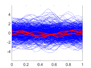
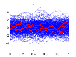
Refer to caption
(a) Inner-product-based Depth
Refer to caption
(b) Modified Half-region Depth
Figure 10: Simulation 3: (a) All 500 simulated functions, where the red curves have the five deepest values obtained by the proposed method. (b) Same as (a) except that the depth values are obtained by the modified half-region depth.

Simulation 6. In this example, we illustrate the norm-based depth on a multivariate data set and compare the Monte Carlo estimate with sample average (as indicated in the beginning of this section). We at first generate n=50𝑛50n=50 random samples in 2superscript2\mathbb{R}^{2} from multivariate normal distribution 𝒩(μ,Σ)𝒩𝜇Σ\mathcal{N}(\mu,\Sigma), where

μ=(00) and Σ=(11/31/31/4).𝜇00 and Σ1131314\mu=\left(\begin{array}[]{c}0\\ 0\end{array}\right)\mbox{ and }\Sigma=\left(\begin{array}[]{cc}1&1/3\\ 1/3&1/4\end{array}\right).

We choose a Mahalanobis distance as the criterion function, that is, for any x2𝑥superscript2x\in\mathbb{R}^{2}, ζ(x,μ)=(xμ)TΣ1(xμ)𝜁𝑥𝜇superscript𝑥𝜇𝑇superscriptΣ1𝑥𝜇\zeta(x,\mu)=\sqrt{(x-\mu)^{T}\Sigma^{-1}(x-\mu)}. Therefore, it is straightforward to derive the closed form of the depth function D(x)=1F(ζ(x,μ)2)𝐷𝑥1𝐹𝜁superscript𝑥𝜇2D(x)=1-F(\zeta(x,\mu)^{2}), where F()𝐹F(\cdot) denotes the cumulative distribution function of chi-square distribution with 2 degrees of freedom.

We compute the depth value for each of these 50 points by Monte-Carlo-based Algorithm I, and then compare the result to the algorithm integrated with sample average of these points. We display these 50 points with color label of their depth values in Figure 11(a). Note that the depth value using the Mahalanobis distance criterion ranges from 0 to 1 and the distirbution of these depth values approximately follow elliptic contours for a two dimensional normal distribution. Since we obtain the closed-form depth values, we can use them to compare the performance of Monte Carlo and sample average method. In Algorithm I, we generate 5000 re-sampling points in step 5. The results in Figure 11 (b)(c) show that the depth values computed by Algorithm I are very close to the theoretical ones, whereas the sample average method does not have the same level of accuracy.
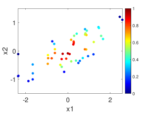
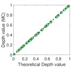
Refer to caption
(a) Given observations
Refer to caption
(b) Depth value comparison 1.
Refer to caption
(c) Depth value comparison 2.
Figure 11: Simulation 4: (a) 50 points from multivariate normal density with color-labeled depth by Algorithm I. (b) Depth value comparison: closed-form depth function (x-axis) vs. Monte-Carlo-based Algorithm I (y-axis) (c) Same as (b) except for sample average method in y-axis.

Appendix D Depth estimation consistency in finite-dimensional data

In this case, P𝑃\exists P\in\mathbb{N} such that λP>0subscript𝜆𝑃0\lambda_{P}>0 and λp=0,p>Pformulae-sequencesubscript𝜆𝑝0for-all𝑝𝑃\lambda_{p}=0,\ \forall\ p>P under the notation setup in Section 4 of the main paper. Then K(s,t)=p=1Pλpϕp(s)ϕp(t)𝐾𝑠𝑡superscriptsubscript𝑝1𝑃subscript𝜆𝑝subscriptitalic-ϕ𝑝𝑠subscriptitalic-ϕ𝑝𝑡K(s,t)=\sum_{p=1}^{P}\lambda_{p}\phi_{p}(s)\phi_{p}(t) and K^(s,t)=p=1nλ^p,nϕ^p,n(s)ϕ^p,n(t)^𝐾𝑠𝑡superscriptsubscript𝑝1𝑛subscript^𝜆𝑝𝑛subscript^italic-ϕ𝑝𝑛𝑠subscript^italic-ϕ𝑝𝑛𝑡\hat{K}(s,t)=\sum_{p=1}^{n}\hat{\lambda}_{p,n}\hat{\phi}_{p,n}(s)\hat{\phi}_{p,n}(t). Therefore, for any fobssubscript𝑓𝑜𝑏𝑠f_{obs}\in\mathcal{F}, we have the squared RKHS induced norm

fobsK2=p=1Pfobs,ϕp2λp<,superscriptsubscriptnormsubscript𝑓𝑜𝑏𝑠subscript𝐾2superscriptsubscript𝑝1𝑃superscriptsubscript𝑓𝑜𝑏𝑠subscriptitalic-ϕ𝑝2subscript𝜆𝑝\|f_{obs}\|_{\mathbb{H}_{K}}^{2}=\sum_{p=1}^{P}\frac{\langle f_{obs},\phi_{p}\rangle^{2}}{\lambda_{p}}<\infty, (13)

where ,\langle\cdot,\cdot\rangle indicates the inner product operation in RKHS with K𝐾K as reproducing kernel.

Based on the RKHS norm, the depth of fobssubscript𝑓𝑜𝑏𝑠f_{obs} is given as follows:

d(fobs)=Dn(fobs,,K,0)=[f:fKfobsK]=1F(fobsK2),d(f_{obs})=D_{n}(f_{obs},\,\mathbb{P},\|\cdot\|_{\mathbb{H}_{K}},0)=\mathbb{P}\big{[}f:\|f\|_{\mathbb{H}_{K}}\geq\|f_{obs}\|_{\mathbb{H}_{K}}\big{]}=1-F(\|f_{obs}\|_{{\mathbb{H}_{K}}}^{2}), (14)

where F(x)𝐹𝑥F(x) denotes the cumulative distribution function of fK2superscriptsubscriptnorm𝑓subscript𝐾2\|f\|_{\mathbb{H}_{K}}^{2} for all f𝑓f\in\mathcal{F}.

As given in Algorithm II in Appendix G, the sample version of the squared modified norm is given as

fobsK^2=p=1nfobs,ϕ^p,n2λ^p,n.superscriptsubscriptnormsubscript𝑓𝑜𝑏𝑠subscript^𝐾2superscriptsubscript𝑝1𝑛superscriptsubscript𝑓𝑜𝑏𝑠subscript^italic-ϕ𝑝𝑛2subscript^𝜆𝑝𝑛\|f_{obs}\|_{{\mathbb{H}_{\hat{K}}}}^{2}=\sum_{p=1}^{n}\frac{\langle f_{obs},\hat{\phi}_{p,n}\rangle^{2}}{\hat{\lambda}_{p,n}}. (15)

Similar to Case I, we adopt the sample version of the depth of fobssubscript𝑓𝑜𝑏𝑠f_{obs}

dn(fobs)=[f:fKfobsK^]=1F(fobsK^2).d_{n}(f_{obs})=\mathbb{P}\big{[}f:\|f\|_{{\mathbb{H}_{K}}}\geq\|f_{obs}\|_{{\mathbb{H}_{\hat{K}}}}\big{]}=1-F(\|f_{obs}\|_{{\mathbb{H}_{\hat{K}}}}^{2}). (16)

We focus on proving dn(fobs)subscript𝑑𝑛subscript𝑓𝑜𝑏𝑠d_{n}(f_{obs}) converges to d(fobs)𝑑subscript𝑓𝑜𝑏𝑠d(f_{obs}) when n𝑛n is large. This is shown in Theorem 4 as follows. In this case, neither a convergent weight series {ap}subscript𝑎𝑝\{a_{p}\} nor Assumption 1 is needed in the proof of consistency.

Theorem 4.

If the covariance kernel K𝐾K has only P()annotated𝑃absentP(\in\mathbb{N}) positive eigenvalues {λp}subscript𝜆𝑝\{\lambda_{p}\}, then we have

supfobs,fobs1|fobsK^2fobsK2|a.s.0.\sup_{f_{obs}\in\mathcal{F},||f_{obs}||\leq 1}|\|f_{obs}\|_{\mathbb{H}_{\hat{K}}}^{2}-\|f_{obs}\|_{\mathbb{H}_{K}}^{2}|\overset{a.s.}{\longrightarrow}0.

Moreover, for any fobssubscript𝑓𝑜𝑏𝑠f_{obs}\in\mathcal{F}

limndn(fobs)=d(fobs).subscript𝑛subscript𝑑𝑛subscript𝑓𝑜𝑏𝑠𝑑subscript𝑓𝑜𝑏𝑠\lim_{n\rightarrow\infty}d_{n}(f_{obs})=d(f_{obs}).

Proof: As convergence almost surely implies convergence in distribution, it is apparent that we only need to prove the first convergence fobsK^2a.s.fobsK2\|f_{obs}\|_{\mathbb{H}_{\hat{K}}}^{2}\overset{a.s.}{\longrightarrow}\|f_{obs}\|_{\mathbb{H}_{K}}^{2}.

Based on the work done by Dauxois et al. (1982) and Bosq (2012), when n𝑛n is large, we have λ^p,na.s.λp>0\hat{\lambda}_{p,n}\overset{a.s.}{\longrightarrow}\lambda_{p}>0 for p{1,,P}𝑝1𝑃p\in\{1,\cdots,P\}, while λ^p,na.s.0\hat{\lambda}_{p,n}\overset{a.s.}{\longrightarrow}0 for p{P+1,,n}𝑝𝑃1𝑛p\in\{P+1,\cdots,n\}(Tran, 2008).

We denote K˘(s,t)=p=1Pλ^p,nϕ^p,n(s)ϕ^p,n(t)˘𝐾𝑠𝑡superscriptsubscript𝑝1𝑃subscript^𝜆𝑝𝑛subscript^italic-ϕ𝑝𝑛𝑠subscript^italic-ϕ𝑝𝑛𝑡\breve{K}(s,t)=\sum_{p=1}^{P}\hat{\lambda}_{p,n}\hat{\phi}_{p,n}(s)\hat{\phi}_{p,n}(t), and we will get K˘K^a.s.0\|\breve{K}-\hat{K}\|\overset{a.s.}{\longrightarrow}0 as n𝑛n\to\infty. Besides, we have K^Ka.s.0\|\hat{K}-K\|\overset{a.s.}{\longrightarrow}0(Dauxois et al., 1982), hence K˘Ka.s.0\|\breve{K}-K\|\overset{a.s.}{\longrightarrow}0.

If we denote K1(s,t)=p=1Pϕp(s)ϕp(t)λpsuperscript𝐾1𝑠𝑡superscriptsubscript𝑝1𝑃subscriptitalic-ϕ𝑝𝑠subscriptitalic-ϕ𝑝𝑡subscript𝜆𝑝K^{-1}(s,t)=\sum_{p=1}^{P}\frac{\phi_{p}(s)\phi_{p}(t)}{\lambda_{p}} and K˘1(s,t)=p=1Pϕ^p,n(s)ϕ^p,n(s)λ^p,nsuperscript˘𝐾1𝑠𝑡superscriptsubscript𝑝1𝑃subscript^italic-ϕ𝑝𝑛𝑠subscript^italic-ϕ𝑝𝑛𝑠subscript^𝜆𝑝𝑛\breve{K}^{-1}(s,t)=\sum_{p=1}^{P}\frac{\hat{\phi}_{p,n}(s)\hat{\phi}_{p,n}(s)}{\hat{\lambda}_{p,n}},

K˘1K1normsuperscript˘𝐾1superscript𝐾1\displaystyle\|\breve{K}^{-1}-K^{-1}\| =K˘1(K˘K)K1absentnormsuperscript˘𝐾1˘𝐾𝐾superscript𝐾1\displaystyle=\|\breve{K}^{-1}(\breve{K}-K)K^{-1}\|
K˘1K˘KK1absentnormsuperscript˘𝐾1norm˘𝐾𝐾normsuperscript𝐾1\displaystyle\leq\|\breve{K}^{-1}\|\|\breve{K}-K\|\|K^{-1}\|
=1λ^p,n1λpK˘Ka.s.0.\displaystyle=\frac{1}{\hat{\lambda}_{p,n}}\frac{1}{\lambda_{p}}\|\breve{K}-K\|\overset{a.s.}{\longrightarrow}0.

In Algorithm 2, the estimated depth is written as

fobsK˘2superscriptsubscriptnormsubscript𝑓𝑜𝑏𝑠subscript˘𝐾2\displaystyle\|f_{obs}\|_{\mathbb{H}_{\breve{K}}}^{2} =p=1Pfobs,ϕ^p,n2λ^p,nabsentsuperscriptsubscript𝑝1𝑃superscriptsubscript𝑓𝑜𝑏𝑠subscript^italic-ϕ𝑝𝑛2subscript^𝜆𝑝𝑛\displaystyle=\sum_{p=1}^{P}\frac{\langle f_{obs},\hat{\phi}_{p,n}\rangle^{2}}{\hat{\lambda}_{p,n}}
=p=1P0101fobs(s)fobs(t)ϕ^p,n(s)ϕ^p,n(s)λ^p,n𝑑s𝑑tabsentsuperscriptsubscript𝑝1𝑃superscriptsubscript01superscriptsubscript01subscript𝑓𝑜𝑏𝑠𝑠subscript𝑓𝑜𝑏𝑠𝑡subscript^italic-ϕ𝑝𝑛𝑠subscript^italic-ϕ𝑝𝑛𝑠subscript^𝜆𝑝𝑛differential-d𝑠differential-d𝑡\displaystyle=\sum_{p=1}^{P}\int_{0}^{1}\int_{0}^{1}f_{obs}(s)f_{obs}(t)\frac{\hat{\phi}_{p,n}(s)\hat{\phi}_{p,n}(s)}{\hat{\lambda}_{p,n}}dsdt
=0101fobs(s)fobs(t)K˘1(s,t)𝑑s𝑑tabsentsuperscriptsubscript01superscriptsubscript01subscript𝑓𝑜𝑏𝑠𝑠subscript𝑓𝑜𝑏𝑠𝑡superscript˘𝐾1𝑠𝑡differential-d𝑠differential-d𝑡\displaystyle=\int_{0}^{1}\int_{0}^{1}f_{obs}(s)f_{obs}(t)\breve{K}^{-1}(s,t)dsdt

Therefore,

|fobsK˘2fobsK2|superscriptsubscriptnormsubscript𝑓𝑜𝑏𝑠subscript˘𝐾2superscriptsubscriptnormsubscript𝑓𝑜𝑏𝑠subscript𝐾2\displaystyle|\ \|f_{obs}\|_{\mathbb{H}_{\breve{K}}}^{2}-\|f_{obs}\|_{\mathbb{H}_{K}}^{2}\ | =|0101fobs(s)fobs(t)K˘1(s,t)𝑑s𝑑t0101fobs(s)fobs(t)K1(s,t)𝑑s𝑑t|absentsuperscriptsubscript01superscriptsubscript01subscript𝑓𝑜𝑏𝑠𝑠subscript𝑓𝑜𝑏𝑠𝑡superscript˘𝐾1𝑠𝑡differential-d𝑠differential-d𝑡superscriptsubscript01superscriptsubscript01subscript𝑓𝑜𝑏𝑠𝑠subscript𝑓𝑜𝑏𝑠𝑡superscript𝐾1𝑠𝑡differential-d𝑠differential-d𝑡\displaystyle=|\ \int_{0}^{1}\int_{0}^{1}f_{obs}(s)f_{obs}(t)\breve{K}^{-1}(s,t)dsdt-\int_{0}^{1}\int_{0}^{1}f_{obs}(s)f_{obs}(t)K^{-1}(s,t)dsdt\ |
=|fobs,(K˘1K1)fobs|absentsubscript𝑓𝑜𝑏𝑠superscript˘𝐾1superscript𝐾1subscript𝑓𝑜𝑏𝑠\displaystyle=|\ \langle f_{obs},(\breve{K}^{-1}-K^{-1})f_{obs}\rangle\ |
fobs2K˘1K1a.s.0.\displaystyle\leq\|f_{obs}\|^{2}\|\breve{K}^{-1}-K^{-1}\|\overset{a.s.}{\longrightarrow}0.

Appendix E Proof of Lemma 1

To better streamline the proof, we first prove the claimed result when the inner-product is induced from the reproducing kernel Hilbert space (RKHS) associated with the covariance function of the GP (which satisfies the Gram matrix condition of the lemma), and then extend the proof to a general inner product. Specifically, we show:

  1. 1.

    (basic form) If we take the induced RKHS (reproducing-kernel Hilbert space) inner-product ,\left<\cdot,\cdot\right> using the covariance function C𝐶C, then

    Dip(fobs,C,,,)=0subscript𝐷𝑖𝑝subscript𝑓𝑜𝑏𝑠subscript𝐶0D_{ip}(f_{obs},\mathbb{P}_{C},\left<\cdot,\cdot\right>,\mathcal{F})=0

    almost surely for fobssubscript𝑓𝑜𝑏𝑠absentf_{obs}\in GP(0,C)0𝐶(0,C)

  2. 2.

    (general form) The above result will in fact hold for any inner-product on \mathcal{F} that satisfies the condition in the lemma.

Proof: (Part 1) Based on the result in Sec 3.1.2, assume the covariance function C(,)𝐶C(\cdot,\cdot) in a Gaussian process GP(0,C)0𝐶(0,C) has infinite number of positive eigenvalues. Then the covariance can be represented as C(s,t)=p=1λpϕp(s)ϕp(t).𝐶𝑠𝑡superscriptsubscript𝑝1subscript𝜆𝑝subscriptitalic-ϕ𝑝𝑠subscriptitalic-ϕ𝑝𝑡C(s,t)=\sum_{p=1}^{\infty}\lambda_{p}\phi_{p}(s)\phi_{p}(t). For any fobsGP(0,C)subscript𝑓𝑜𝑏𝑠𝐺𝑃0𝐶f_{obs}\in GP(0,C), let fobs,p=01fobs(s)ϕp(s)𝑑ssubscript𝑓𝑜𝑏𝑠𝑝superscriptsubscript01subscript𝑓𝑜𝑏𝑠𝑠subscriptitalic-ϕ𝑝𝑠differential-d𝑠f_{obs,p}=\int_{0}^{1}f_{obs}(s)\phi_{p}(s)ds. We have fobs(t)=p=1fobs,pϕp(t)subscript𝑓𝑜𝑏𝑠𝑡superscriptsubscript𝑝1subscript𝑓𝑜𝑏𝑠𝑝subscriptitalic-ϕ𝑝𝑡f_{obs}(t)=\sum_{p=1}^{\infty}f_{obs,p}\phi_{p}(t). Hence, the induced RKHS norm

fobsC=p=1fobs,p2λp=(a.s.)\|f_{o}bs\|_{\mathbb{H}_{C}}=\sum_{p=1}^{\infty}\frac{f_{obs,p}^{2}}{\lambda_{p}}=\infty\ \ \ (a.s.)

For any integer P>0𝑃0P>0 and function f𝑓f\in\mathcal{F}, we let fPsuperscript𝑓𝑃f^{P} represent the finite cutoff of f𝑓f at the P𝑃P-th order. That is, fP(t)=p=1Pfpϕp(t)superscript𝑓𝑃𝑡superscriptsubscript𝑝1𝑃subscript𝑓𝑝subscriptitalic-ϕ𝑝𝑡f^{P}(t)=\sum_{p=1}^{P}f_{p}\phi_{p}(t). Let 𝒢Psubscript𝒢𝑃\mathcal{G}_{P} denote the finite-dimensional space expanded by {ϕp(t)}p=1Psuperscriptsubscriptsubscriptitalic-ϕ𝑝𝑡𝑝1𝑃\{\phi_{p}(t)\}_{p=1}^{P}. Using the result in Appendix A, the inner-product depth

Dip(fobsP,C,,,𝒢P)=1Φ(fobsPC).subscript𝐷𝑖𝑝subscriptsuperscript𝑓𝑃𝑜𝑏𝑠subscript𝐶subscript𝒢𝑃1Φsubscriptnormsubscriptsuperscript𝑓𝑃𝑜𝑏𝑠subscript𝐶D_{ip}(f^{P}_{obs},\mathbb{P}_{C},\left<\cdot,\cdot\right>,\mathcal{G}_{P})=1-\Phi(\|f^{P}_{obs}\|_{\mathbb{H}_{C}}). (17)

Note that fobsPC=p=1Pfobs,p2λp(a.s.)\|f^{P}_{obs}\|_{\mathbb{H}_{C}}=\sum_{p=1}^{P}\frac{f_{obs,p}^{2}}{\lambda_{p}}\rightarrow\infty(a.s.) as P𝑃P\rightarrow\infty. Then 1Φ(fobsPC)1Φ()=11=0(a.s.)1-\Phi(\|f^{P}_{obs}\|_{\mathbb{H}_{C}})\rightarrow 1-\Phi(\infty)=1-1=0\ \ (a.s.) Finally, we have

Dip(fobs,C,,,)infPDip(fobsP,C,,,𝒢P)0.(a.s.)D_{ip}(f_{obs},\mathbb{P}_{C},\left<\cdot,\cdot\right>,\mathcal{F})\leq\inf_{P}D_{ip}(f^{P}_{obs},\mathbb{P}_{C},\left<\cdot,\cdot\right>,\mathcal{G}_{P})\rightarrow 0.\ \ \ (a.s.)

(Part 2) We see that the proof of Part 1 mainly relies on the result in Appendix A (Equation (17)), where we use the induced RKHS inner-product. Let f𝑓f be a realization from the Gaussian process GP(0,C)0𝐶(0,C). Here we just need to show that using the new inner-product, such equation will still hold. Again, we consider the finite cut-off of fobsPsubscriptsuperscript𝑓𝑃𝑜𝑏𝑠f^{P}_{obs} at the P𝑃P-th order, and will show that Equation (17) remains valid with the new inner product ,\langle\cdot,\cdot\rangle. Therefore, we suppress the superscript P𝑃P in proving this equation in the rest of this part. Under this notation, we can write

f(t)𝑓𝑡\displaystyle f(t) =p=1Pfpϕp(t)K,absentsuperscriptsubscript𝑝1𝑃subscript𝑓𝑝subscriptitalic-ϕ𝑝𝑡subscript𝐾\displaystyle=\sum_{p=1}^{P}f_{p}\phi_{p}(t)\in\mathbb{H}_{K},
g(t)𝑔𝑡\displaystyle g(t) =p=1Pgpϕp(t)K,absentsuperscriptsubscript𝑝1𝑃subscript𝑔𝑝subscriptitalic-ϕ𝑝𝑡subscript𝐾\displaystyle=\sum_{p=1}^{P}g_{p}\phi_{p}(t)\in\mathbb{H}_{K},
fobs(t)subscript𝑓𝑜𝑏𝑠𝑡\displaystyle f_{obs}(t) =p=1Pfobs,pϕp(t)𝟎K,absentsuperscriptsubscript𝑝1𝑃subscript𝑓𝑜𝑏𝑠𝑝subscriptitalic-ϕ𝑝𝑡0subscript𝐾\displaystyle=\sum_{p=1}^{P}f_{obs,p}\phi_{p}(t)\neq{\bf 0}\in\mathbb{H}_{K},

where fpsubscript𝑓𝑝f_{p} are independent normal random variables with 𝔼fp=0𝔼subscript𝑓𝑝0\mathbb{E}f_{p}=0 and Varfp=λp,p=1,,Pformulae-sequence𝑉𝑎𝑟subscript𝑓𝑝subscript𝜆𝑝𝑝1𝑃Varf_{p}=\lambda_{p},p=1,\cdots,P.

For this new inner-product ,\left<\cdot,\cdot\right> on \mathcal{F}, let rij=ϕi,ϕjsubscript𝑟𝑖𝑗subscriptitalic-ϕ𝑖subscriptitalic-ϕ𝑗r_{ij}=\left<\phi_{i},\phi_{j}\right> for 1i,jPformulae-sequence1𝑖𝑗𝑃1\leq i,j\leq P. We also denote

X=ffobs,g=i=1Pj=1P(fifobs,i)gjrij=i=1Pj=1Pfobs,igjrij+i=1Pj=1Pfigjrij.𝑋𝑓subscript𝑓𝑜𝑏𝑠𝑔superscriptsubscript𝑖1𝑃superscriptsubscript𝑗1𝑃subscript𝑓𝑖subscript𝑓𝑜𝑏𝑠𝑖subscript𝑔𝑗subscript𝑟𝑖𝑗superscriptsubscript𝑖1𝑃superscriptsubscript𝑗1𝑃subscript𝑓𝑜𝑏𝑠𝑖subscript𝑔𝑗subscript𝑟𝑖𝑗superscriptsubscript𝑖1𝑃superscriptsubscript𝑗1𝑃subscript𝑓𝑖subscript𝑔𝑗subscript𝑟𝑖𝑗\displaystyle X=\left<f-f_{obs},g\right>=\sum_{i=1}^{P}\sum_{j=1}^{P}(f_{i}-f_{obs,i})g_{j}r_{ij}=-\sum_{i=1}^{P}\sum_{j=1}^{P}f_{obs,i}g_{j}r_{ij}+\sum_{i=1}^{P}\sum_{j=1}^{P}f_{i}g_{j}r_{ij}.

It is straightforward to know that X𝑋X is normally distributed with 𝔼X=i=1Pj=1Pfobs,igjrij:=μg\mathbb{E}X=-\sum_{i=1}^{P}\sum_{j=1}^{P}f_{obs,i}g_{j}r_{ij}:\,=\mu_{g} and VarX=i=1P(j=1Pgjrij)2λi:=σg2VarX=\sum_{i=1}^{P}(\sum_{j=1}^{P}g_{j}r_{ij})^{2}\lambda_{i}:\,=\sigma_{g}^{2}. Now we can compute the probability

θ[ffobs,g0]=θ[X0]=θ[Xμgσgμgσg]=1θ[Xμgσgμgσg].subscript𝜃delimited-[]𝑓subscript𝑓𝑜𝑏𝑠𝑔0subscript𝜃delimited-[]𝑋0subscript𝜃delimited-[]𝑋subscript𝜇𝑔subscript𝜎𝑔subscript𝜇𝑔subscript𝜎𝑔1subscript𝜃delimited-[]𝑋subscript𝜇𝑔subscript𝜎𝑔subscript𝜇𝑔subscript𝜎𝑔\displaystyle\mathbb{P}_{\theta}\big{[}\left<f-f_{obs},g\right>\geq 0\big{]}=\mathbb{P}_{\theta}\big{[}X\geq 0\big{]}=\mathbb{P}_{\theta}\big{[}\frac{X-\mu_{g}}{\sigma_{g}}\geq-\frac{\mu_{g}}{\sigma_{g}}\big{]}=1-\mathbb{P}_{\theta}\big{[}\frac{X-\mu_{g}}{\sigma_{g}}\leq-\frac{\mu_{g}}{\sigma_{g}}\big{]}.

With the normal assumption, θ[ffobs,gmod0]=1Φ(μgσg)subscript𝜃delimited-[]subscript𝑓subscript𝑓𝑜𝑏𝑠𝑔𝑚𝑜𝑑01Φsubscript𝜇𝑔subscript𝜎𝑔\mathbb{P}_{\theta}\big{[}\left<f-f_{obs},g\right>_{mod}\geq 0\big{]}=1-\Phi(-\frac{\mu_{g}}{\sigma_{g}}) where ΦΦ\Phi is the c.d.f. of a standard normal random variable Xμgσg𝑋subscript𝜇𝑔subscript𝜎𝑔\frac{X-\mu_{g}}{\sigma_{g}} (it does not depend on g𝑔g). To minimize the probability with respect to g𝑔g, we need to maximize μg/σgsubscript𝜇𝑔subscript𝜎𝑔-\mu_{g}/\sigma_{g}, or μg2/σg2superscriptsubscript𝜇𝑔2subscriptsuperscript𝜎2𝑔\mu_{g}^{2}/\sigma^{2}_{g}.

By the Cauchy inequality, we have

μg2σg2superscriptsubscript𝜇𝑔2subscriptsuperscript𝜎2𝑔\displaystyle\frac{\mu_{g}^{2}}{\sigma^{2}_{g}} =(i=1Pj=1Pfobs,igjrij)2i=1P(j=1Pgjrij)2λi=(i=1Pfobs,iλiλij=1Pgjrij)2i=1P(j=1Pgjrij)2λiabsentsuperscriptsuperscriptsubscript𝑖1𝑃superscriptsubscript𝑗1𝑃subscript𝑓𝑜𝑏𝑠𝑖subscript𝑔𝑗subscript𝑟𝑖𝑗2superscriptsubscript𝑖1𝑃superscriptsuperscriptsubscript𝑗1𝑃subscript𝑔𝑗subscript𝑟𝑖𝑗2subscript𝜆𝑖superscriptsuperscriptsubscript𝑖1𝑃subscript𝑓𝑜𝑏𝑠𝑖subscript𝜆𝑖subscript𝜆𝑖superscriptsubscript𝑗1𝑃subscript𝑔𝑗subscript𝑟𝑖𝑗2superscriptsubscript𝑖1𝑃superscriptsuperscriptsubscript𝑗1𝑃subscript𝑔𝑗subscript𝑟𝑖𝑗2subscript𝜆𝑖\displaystyle=\frac{(\sum_{i=1}^{P}\sum_{j=1}^{P}f_{obs,i}g_{j}r_{ij})^{2}}{\sum_{i=1}^{P}(\sum_{j=1}^{P}g_{j}r_{ij})^{2}\lambda_{i}}=\frac{(\sum_{i=1}^{P}\frac{f_{obs,i}}{\sqrt{\lambda_{i}}}\sqrt{\lambda_{i}}\sum_{j=1}^{P}g_{j}r_{ij})^{2}}{\sum_{i=1}^{P}(\sum_{j=1}^{P}g_{j}r_{ij})^{2}\lambda_{i}}
i=1P(fobs,iλi)2i=1P(λij=1Pgjrij)2i=1P(j=1Pgjrij)2λi=ifobs,i2λiabsentsuperscriptsubscript𝑖1𝑃superscriptsubscript𝑓𝑜𝑏𝑠𝑖subscript𝜆𝑖2superscriptsubscript𝑖1𝑃superscriptsubscript𝜆𝑖superscriptsubscript𝑗1𝑃subscript𝑔𝑗subscript𝑟𝑖𝑗2superscriptsubscript𝑖1𝑃superscriptsuperscriptsubscript𝑗1𝑃subscript𝑔𝑗subscript𝑟𝑖𝑗2subscript𝜆𝑖subscript𝑖superscriptsubscript𝑓𝑜𝑏𝑠𝑖2subscript𝜆𝑖\displaystyle\leq\frac{\sum_{i=1}^{P}(\frac{f_{obs,i}}{\sqrt{\lambda_{i}}})^{2}\sum_{i=1}^{P}(\sqrt{\lambda_{i}}\sum_{j=1}^{P}g_{j}r_{ij})^{2}}{\sum_{i=1}^{P}(\sum_{j=1}^{P}g_{j}r_{ij})^{2}\lambda_{i}}=\sum_{i}\frac{f_{obs,i}^{2}}{\lambda_{i}}

The equality holds if and only if there exists c>0𝑐0c>0 such that cfobs,iλi=λij=1Pgjrij,i=1,,Pformulae-sequence𝑐subscript𝑓𝑜𝑏𝑠𝑖subscript𝜆𝑖subscript𝜆𝑖superscriptsubscript𝑗1𝑃subscript𝑔𝑗subscript𝑟𝑖𝑗𝑖1𝑃c\frac{f_{obs,i}}{\sqrt{\lambda_{i}}}=\sqrt{\lambda_{i}}\sum_{j=1}^{P}g_{j}r_{ij},i=1,\cdots,P. That is,

j=1Pgjrij=cfobs,iλi,i=1,2,,P.formulae-sequencesuperscriptsubscript𝑗1𝑃subscript𝑔𝑗subscript𝑟𝑖𝑗𝑐subscript𝑓𝑜𝑏𝑠𝑖subscript𝜆𝑖𝑖12𝑃\sum_{j=1}^{P}g_{j}r_{ij}=c\frac{f_{obs,i}}{\lambda_{i}},\ \ i=1,2,\ldots,P.

Under the condition on the inner-product in the lemma, this set of linear equations always admits a unique solution. By plugging-in this solution, the maximum of μgσgsubscript𝜇𝑔subscript𝜎𝑔-\frac{\mu_{g}}{\sigma_{g}} is obtained at

i=1Pfobs,ij=1Pgjriji=1P(j=1Pgjrij)2λi=i=1Pfobs,icfobs,iλii=1P(cfobs,iλi)2λi=i=1Pfobs,i2λi=fobsC.superscriptsubscript𝑖1𝑃subscript𝑓𝑜𝑏𝑠𝑖superscriptsubscript𝑗1𝑃subscript𝑔𝑗subscript𝑟𝑖𝑗superscriptsubscript𝑖1𝑃superscriptsuperscriptsubscript𝑗1𝑃subscript𝑔𝑗subscript𝑟𝑖𝑗2subscript𝜆𝑖superscriptsubscript𝑖1𝑃subscript𝑓𝑜𝑏𝑠𝑖𝑐subscript𝑓𝑜𝑏𝑠𝑖subscript𝜆𝑖superscriptsubscript𝑖1𝑃superscript𝑐subscript𝑓𝑜𝑏𝑠𝑖subscript𝜆𝑖2subscript𝜆𝑖superscriptsubscript𝑖1𝑃superscriptsubscript𝑓𝑜𝑏𝑠𝑖2subscript𝜆𝑖subscriptnormsubscript𝑓𝑜𝑏𝑠subscript𝐶\displaystyle-\frac{-\sum_{i=1}^{P}f_{obs,i}\sum_{j=1}^{P}g_{j}r_{ij}}{\sqrt{\sum_{i=1}^{P}(\sum_{j=1}^{P}g_{j}r_{ij})^{2}\lambda_{i}}}=\frac{\sum_{i=1}^{P}f_{obs,i}c\frac{f_{obs,i}}{\lambda_{i}}}{\sqrt{\sum_{i=1}^{P}(c\frac{f_{obs,i}}{\lambda_{i}})^{2}\lambda_{i}}}=\sqrt{\sum_{i=1}^{P}\frac{f_{obs,i}^{2}}{\lambda_{i}}}=\|f_{obs}\|_{\mathbb{H}_{C}}.

Finally, the depth of fobssubscript𝑓𝑜𝑏𝑠f_{obs} is still given in the following form:

Dip(fobs,θ,,,)=1Φ(fobsC).subscript𝐷𝑖𝑝subscript𝑓𝑜𝑏𝑠subscript𝜃1Φsubscriptnormsubscript𝑓𝑜𝑏𝑠subscript𝐶D_{ip}(f_{obs},\,\mathbb{P}_{\theta},\left<\cdot,\cdot\right>,\mathcal{F})=1-\Phi(\|f_{obs}\|_{\mathbb{H}_{C}}).

Appendix F Optimal solution of depth with inner-product-based criterion

We assume that f(𝕃2([0,1]))𝑓annotatedabsentsuperscript𝕃201f\in\mathcal{F}(\subset\mathbb{L}^{2}([0,1])) is random realizations from one zero-mean Gaussian process with covariance kernel K𝐾K in a finite Karhunen Loève expansion K(s,t)=p=1Pλpϕp(s)ϕp(t),s,t[0,1]formulae-sequence𝐾𝑠𝑡superscriptsubscript𝑝1𝑃subscript𝜆𝑝subscriptitalic-ϕ𝑝𝑠subscriptitalic-ϕ𝑝𝑡𝑠𝑡01K(s,t)=\sum_{p=1}^{P}\lambda_{p}\phi_{p}(s)\phi_{p}(t),s,t\in[0,1]. As discussed in Sec. 3.1.2, the realizations from the Gaussian process form an RKHS Ksubscript𝐾\mathbb{H}_{K}. Let

f(t)𝑓𝑡\displaystyle f(t) =p=1Pfpϕp(t)K,absentsuperscriptsubscript𝑝1𝑃subscript𝑓𝑝subscriptitalic-ϕ𝑝𝑡subscript𝐾\displaystyle=\sum_{p=1}^{P}f_{p}\phi_{p}(t)\in\mathbb{H}_{K},
g(t)𝑔𝑡\displaystyle g(t) =p=1Pgpϕp(t)K,absentsuperscriptsubscript𝑝1𝑃subscript𝑔𝑝subscriptitalic-ϕ𝑝𝑡subscript𝐾\displaystyle=\sum_{p=1}^{P}g_{p}\phi_{p}(t)\in\mathbb{H}_{K},
fobs(t)subscript𝑓𝑜𝑏𝑠𝑡\displaystyle f_{obs}(t) =p=1Pfobs,pϕp(t)𝟎K,absentsuperscriptsubscript𝑝1𝑃subscript𝑓𝑜𝑏𝑠𝑝subscriptitalic-ϕ𝑝𝑡0subscript𝐾\displaystyle=\sum_{p=1}^{P}f_{obs,p}\phi_{p}(t)\neq{\bf 0}\in\mathbb{H}_{K},

where fpsubscript𝑓𝑝f_{p} are independent normal random variables with 𝔼fp=0𝔼subscript𝑓𝑝0\mathbb{E}f_{p}=0 and Varfp=λp,p=1,,Pformulae-sequence𝑉𝑎𝑟subscript𝑓𝑝subscript𝜆𝑝𝑝1𝑃Varf_{p}=\lambda_{p},p=1,\cdots,P.

Using the inner-product, we denote

X=ffobs,gK=p=1P(fpfobs,p)gpλp=p=1Pfobs,pgpλp+p=1Pfpgpλp.𝑋subscript𝑓subscript𝑓𝑜𝑏𝑠𝑔subscript𝐾superscriptsubscript𝑝1𝑃subscript𝑓𝑝subscript𝑓𝑜𝑏𝑠𝑝subscript𝑔𝑝subscript𝜆𝑝superscriptsubscript𝑝1𝑃subscript𝑓𝑜𝑏𝑠𝑝subscript𝑔𝑝subscript𝜆𝑝superscriptsubscript𝑝1𝑃subscript𝑓𝑝subscript𝑔𝑝subscript𝜆𝑝\displaystyle X=\left<f-f_{obs},g\right>_{\mathbb{H}_{K}}=\sum_{p=1}^{P}\frac{(f_{p}-f_{obs,p})g_{p}}{\lambda_{p}}=-\sum_{p=1}^{P}\frac{f_{obs,p}g_{p}}{\lambda_{p}}+\sum_{p=1}^{P}\frac{f_{p}g_{p}}{\lambda_{p}}.

It is straightforward to know that X𝑋X is normally distributed with 𝔼X=p=1Pfobs,pgpλp:=μg\mathbb{E}X=-\sum_{p=1}^{P}\frac{f_{obs,p}g_{p}}{\lambda_{p}}:\,=\mu_{g} and VarX=p=1Pgp2λp:=σg2VarX=\sum_{p=1}^{P}\frac{g_{p}^{2}}{\lambda_{p}}:\,=\sigma_{g}^{2}. Now we can compute the probability

θ[ffobs,gK0]=θ[X0]=θ[Xμgσgμgσg]=1θ[Xμgσgμgσg].subscript𝜃delimited-[]subscript𝑓subscript𝑓𝑜𝑏𝑠𝑔subscript𝐾0subscript𝜃delimited-[]𝑋0subscript𝜃delimited-[]𝑋subscript𝜇𝑔subscript𝜎𝑔subscript𝜇𝑔subscript𝜎𝑔1subscript𝜃delimited-[]𝑋subscript𝜇𝑔subscript𝜎𝑔subscript𝜇𝑔subscript𝜎𝑔\displaystyle\mathbb{P}_{\theta}\big{[}\left<f-f_{obs},g\right>_{\mathbb{H}_{K}}\geq 0\big{]}=\mathbb{P}_{\theta}\big{[}X\geq 0\big{]}=\mathbb{P}_{\theta}\big{[}\frac{X-\mu_{g}}{\sigma_{g}}\geq-\frac{\mu_{g}}{\sigma_{g}}\big{]}=1-\mathbb{P}_{\theta}\big{[}\frac{X-\mu_{g}}{\sigma_{g}}\leq-\frac{\mu_{g}}{\sigma_{g}}\big{]}.

With the normal assumption, θ[ffobs,gK0]=1Φ(μgσg)subscript𝜃delimited-[]subscript𝑓subscript𝑓𝑜𝑏𝑠𝑔subscript𝐾01Φsubscript𝜇𝑔subscript𝜎𝑔\mathbb{P}_{\theta}\big{[}\left<f-f_{obs},g\right>_{\mathbb{H}_{K}}\geq 0\big{]}=1-\Phi(-\frac{\mu_{g}}{\sigma_{g}}) where ΦΦ\Phi is the c.d.f. of a standard normal random variable Xμgσg𝑋subscript𝜇𝑔subscript𝜎𝑔\frac{X-\mu_{g}}{\sigma_{g}} (it does not depend on g𝑔g). To minimize the probability with respect to g𝑔g, we need to maximize μg/σgsubscript𝜇𝑔subscript𝜎𝑔-\mu_{g}/\sigma_{g}, or μg2/σg2superscriptsubscript𝜇𝑔2subscriptsuperscript𝜎2𝑔\mu_{g}^{2}/\sigma^{2}_{g}.

Let

ap=fobs,pλp,bp=1λp.formulae-sequencesubscript𝑎𝑝subscript𝑓𝑜𝑏𝑠𝑝subscript𝜆𝑝subscript𝑏𝑝1subscript𝜆𝑝a_{p}=\frac{f_{obs,p}}{\lambda_{p}},b_{p}=\frac{1}{\sqrt{\lambda_{p}}}.

Then use the Cauchy inequality,

μg2σg2superscriptsubscript𝜇𝑔2subscriptsuperscript𝜎2𝑔\displaystyle\frac{\mu_{g}^{2}}{\sigma^{2}_{g}} =(papgp)2pbp2gp2=(papbpbpgp)2pbp2gp2p(apbp)2p(bpgp)2pbp2gp2=p=1P(apbp)2.absentsuperscriptsubscript𝑝subscript𝑎𝑝subscript𝑔𝑝2subscript𝑝superscriptsubscript𝑏𝑝2superscriptsubscript𝑔𝑝2superscriptsubscript𝑝subscript𝑎𝑝subscript𝑏𝑝subscript𝑏𝑝subscript𝑔𝑝2subscript𝑝superscriptsubscript𝑏𝑝2superscriptsubscript𝑔𝑝2subscript𝑝superscriptsubscript𝑎𝑝subscript𝑏𝑝2subscript𝑝superscriptsubscript𝑏𝑝subscript𝑔𝑝2subscript𝑝superscriptsubscript𝑏𝑝2superscriptsubscript𝑔𝑝2superscriptsubscript𝑝1𝑃superscriptsubscript𝑎𝑝subscript𝑏𝑝2\displaystyle=\frac{(\sum_{p}a_{p}g_{p})^{2}}{\sum_{p}b_{p}^{2}g_{p}^{2}}=\frac{(\sum_{p}\frac{a_{p}}{b_{p}}b_{p}g_{p})^{2}}{\sum_{p}b_{p}^{2}g_{p}^{2}}\leq\frac{\sum_{p}(\frac{a_{p}}{b_{p}})^{2}\sum_{p}(b_{p}g_{p})^{2}}{\sum_{p}b_{p}^{2}g_{p}^{2}}=\sum_{p=1}^{P}(\frac{a_{p}}{b_{p}})^{2}.

The equality holds if and only if there exists c>0𝑐0c>0 such that capbp=bpgp,p=1,,Pformulae-sequence𝑐subscript𝑎𝑝subscript𝑏𝑝subscript𝑏𝑝subscript𝑔𝑝𝑝1𝑃c\frac{a_{p}}{b_{p}}=b_{p}g_{p},p=1,\cdots,P. That is,

gp=capbp2=cfobs,pλpλp=cfobs,p.subscript𝑔𝑝𝑐subscript𝑎𝑝superscriptsubscript𝑏𝑝2𝑐subscript𝑓𝑜𝑏𝑠𝑝subscript𝜆𝑝subscript𝜆𝑝𝑐subscript𝑓𝑜𝑏𝑠𝑝g_{p}=c\frac{a_{p}}{b_{p}^{2}}=c\cdot\frac{f_{obs,p}}{\lambda_{p}}\cdot\lambda_{p}=cf_{obs,p}.

With the constraint gK=1subscriptnorm𝑔subscript𝐾1||g||_{\mathbb{H}_{K}}=1,

1=g,gK=p=1Pgp2λk=p=1Pc2fobs,p2λp=c2p=1Pfobs,p2λp=c2fobsK2.1subscript𝑔𝑔subscript𝐾superscriptsubscript𝑝1𝑃superscriptsubscript𝑔𝑝2subscript𝜆𝑘superscriptsubscript𝑝1𝑃superscript𝑐2superscriptsubscript𝑓𝑜𝑏𝑠𝑝2subscript𝜆𝑝superscript𝑐2superscriptsubscript𝑝1𝑃superscriptsubscript𝑓𝑜𝑏𝑠𝑝2subscript𝜆𝑝superscript𝑐2superscriptsubscriptnormsubscript𝑓𝑜𝑏𝑠subscript𝐾21=\left<g,g\right>_{\mathbb{H}_{K}}=\sum_{p=1}^{P}\frac{g_{p}^{2}}{\lambda_{k}}=\sum_{p=1}^{P}\frac{c^{2}f_{obs,p}^{2}}{\lambda_{p}}=c^{2}\sum_{p=1}^{P}\frac{f_{obs,p}^{2}}{\lambda_{p}}=c^{2}\|f_{obs}\|_{\mathbb{H}_{K}}^{2}.

Therefore, c2=1fobsK2superscript𝑐21superscriptsubscriptnormsubscript𝑓𝑜𝑏𝑠subscript𝐾2c^{2}=\frac{1}{\|f_{obs}\|_{\mathbb{H}_{K}}^{2}} and gp=fobs,pfobsKsubscript𝑔𝑝subscript𝑓𝑜𝑏𝑠𝑝subscriptnormsubscript𝑓𝑜𝑏𝑠subscript𝐾g_{p}=\frac{f_{obs,p}}{\|f_{obs}\|_{\mathbb{H}_{K}}}. We have found the optimal solution

g(t)=arginfg,gK=1θ[ffobs,gK0]=p=1Pfobs,pfobsKϕp(t)=fobs(t)fobsK.superscript𝑔𝑡subscriptarginfformulae-sequence𝑔subscriptnorm𝑔subscript𝐾1subscript𝜃delimited-[]subscript𝑓subscript𝑓𝑜𝑏𝑠𝑔subscript𝐾0superscriptsubscript𝑝1𝑃subscript𝑓𝑜𝑏𝑠𝑝subscriptnormsubscript𝑓𝑜𝑏𝑠subscript𝐾subscriptitalic-ϕ𝑝𝑡subscript𝑓𝑜𝑏𝑠𝑡subscriptnormsubscript𝑓𝑜𝑏𝑠subscript𝐾g^{\ast}(t)=\mbox{arginf}_{g\in\mathcal{F},||g||_{\mathbb{H}_{K}}=1}\mathbb{P}_{\theta}\big{[}\left<f-f_{obs},g\right>_{\mathbb{H}_{K}}\geq 0\big{]}=\sum_{p=1}^{P}\frac{f_{obs,p}}{\|f_{obs}\|_{\mathbb{H}_{K}}}\phi_{p}(t)=\frac{f_{obs}(t)}{\|f_{obs}\|_{\mathbb{H}_{K}}}.

With this optimal gsuperscript𝑔g^{*},

μgσg=p=1Pfobs,pgpλpp=1Pgp2λp=p=1Pfobs,pλpfobs,pfobsKp=1Pfobs,p2fobsK21λp=fobsK.subscript𝜇superscript𝑔subscript𝜎superscript𝑔superscriptsubscript𝑝1𝑃subscript𝑓𝑜𝑏𝑠𝑝subscript𝑔𝑝subscript𝜆𝑝superscriptsubscript𝑝1𝑃superscriptsubscript𝑔𝑝2subscript𝜆𝑝superscriptsubscript𝑝1𝑃subscript𝑓𝑜𝑏𝑠𝑝subscript𝜆𝑝subscript𝑓𝑜𝑏𝑠𝑝subscriptnormsubscript𝑓𝑜𝑏𝑠subscript𝐾superscriptsubscript𝑝1𝑃superscriptsubscript𝑓𝑜𝑏𝑠𝑝2superscriptsubscriptnormsubscript𝑓𝑜𝑏𝑠subscript𝐾21subscript𝜆𝑝subscriptnormsubscript𝑓𝑜𝑏𝑠subscript𝐾\displaystyle-\frac{\mu_{g^{*}}}{\sigma_{g^{*}}}=-\frac{-\sum_{p=1}^{P}\frac{f_{obs,p}g_{p}}{\lambda_{p}}}{\sqrt{\sum_{p=1}^{P}\frac{g_{p}^{2}}{\lambda_{p}}}}=\frac{\sum_{p=1}^{P}\frac{f_{obs,p}}{\lambda_{p}}\cdot\frac{f_{obs,p}}{\|f_{obs}\|_{\mathbb{H}_{K}}}}{\sqrt{\sum_{p=1}^{P}\frac{f_{obs,p}^{2}}{\|f_{obs}\|_{\mathbb{H}_{K}}^{2}}\cdot\frac{1}{\lambda_{p}}}}=\|f_{obs}\|_{\mathbb{H}_{K}}.

Finally, the depth of fobssubscript𝑓𝑜𝑏𝑠f_{obs} is given in the following form:

Dip(fobs):=Dip(fobs,θ,,,)=1Φ(fobsK).assignsubscript𝐷𝑖𝑝subscript𝑓𝑜𝑏𝑠subscript𝐷𝑖𝑝subscript𝑓𝑜𝑏𝑠subscript𝜃1Φsubscriptnormsubscript𝑓𝑜𝑏𝑠subscript𝐾D_{ip}(f_{obs}):=D_{ip}(f_{obs},\,\mathbb{P}_{\theta},\left<\cdot,\cdot\right>,\mathcal{F})=1-\Phi(\|f_{obs}\|_{\mathbb{H}_{K}}).

Appendix G Proof of Lemma 2

Proof: 1) norm-based depth in general form:

  • P-2: By definition, the general depth Dn(fobs,θ,,fc)D_{n}(f_{obs},\,\mathbb{P}_{\theta},\|\cdot\|,f_{c}) is strictly decreasing with respect to fobsfcnormsubscript𝑓𝑜𝑏𝑠subscript𝑓𝑐\|f_{obs}-f_{c}\|. As fobsfcfcfc=0normsubscript𝑓𝑜𝑏𝑠subscript𝑓𝑐normsubscript𝑓𝑐subscript𝑓𝑐0\|f_{obs}-f_{c}\|\geq\|f_{c}-f_{c}\|=0, we have Dn(fobs,θ,,fc)Dn(fc,θ,,fc).D_{n}(f_{obs},\,\mathbb{P}_{\theta},\|\cdot\|,f_{c})\geq D_{n}(f_{c},\,\mathbb{P}_{\theta},\|\cdot\|,f_{c}).

  • P-3: For any α(0,1)𝛼01\alpha\in(0,1), fc+α(fobsfc)fc=αfobsfcfobsfcnormsubscript𝑓𝑐𝛼subscript𝑓𝑜𝑏𝑠subscript𝑓𝑐subscript𝑓𝑐𝛼normsubscript𝑓𝑜𝑏𝑠subscript𝑓𝑐normsubscript𝑓𝑜𝑏𝑠subscript𝑓𝑐\|f_{c}+\alpha(f_{obs}-f_{c})-f_{c}\|=\alpha\|f_{obs}-f_{c}\|\leq\|f_{obs}-f_{c}\|. By Definition 1, Dn(fc+α(fobsfc),θ,s,fc)Dn(fobs,θ,,fc).D_{n}(f_{c}+\alpha(f_{obs}-f_{c}),\,\mathbb{P}_{\theta},s,f_{c})\geq D_{n}(f_{obs},\,\mathbb{P}_{\theta},\|\cdot\|,f_{c}).

  • P-4: Obvious.

2) norm-based depth in specific form:

  • P-1: Dn(afobs+h,θ,aF+h,,afc+h)=θ[f:af+h(afc+h)afobs+h(afc+h)]=θ[f:ffcfobsfc]=Dn(fobs,θ,F,,fc)D_{n}(af_{obs}+h,\,\mathbb{P}_{\theta,aF+h},\|\cdot\|,af_{c}+h)=\mathbb{P}_{\theta}\big{[}f:\|af+h-(af_{c}+h)\|\geq\|af_{obs}+h-(af_{c}+h)\|\big{]}=\mathbb{P}_{\theta}\big{[}f:\|f-f_{c}\|\geq\|f_{obs}-f_{c}\|\big{]}=D_{n}(f_{obs},\,\mathbb{P}_{\theta,F},\|\cdot\|,f_{c})

  • P-2: Dn(fobs,θ,,fc)=θ[f:ffcfobsfc]θ[f:ffc0]=Dn(fc,θ,,fc)D_{n}(f_{obs},\,\mathbb{P}_{\theta},\|\cdot\|,f_{c})=\mathbb{P}_{\theta}\big{[}f:\|f-f_{c}\|\geq\|f_{obs}-f_{c}\|\big{]}\leq\mathbb{P}_{\theta}\big{[}f:\|f-f_{c}\|\geq 0\big{]}=D_{n}(f_{c},\,\mathbb{P}_{\theta},\|\cdot\|,f_{c})

  • P-3: For any α(0,1)𝛼01\alpha\in(0,1), Dn(fc+α(fobsfc),θ,s,fc)=θ[f:ffcfc+α(fobsfc)fc]=θ[f:ffcα(fobsfc)]θ[f:ffcfobsfc]=Dn(fobs,θ,,fc).D_{n}(f_{c}+\alpha(f_{obs}-f_{c}),\,\mathbb{P}_{\theta},s,f_{c})=\mathbb{P}_{\theta}\big{[}f:\|f-f_{c}\|\geq\|f_{c}+\alpha(f_{obs}-f_{c})-f_{c}\|\big{]}=\mathbb{P}_{\theta}\big{[}f:\|f-f_{c}\|\geq\alpha\|(f_{obs}-f_{c})\|\big{]}\geq\mathbb{P}_{\theta}\big{[}f:\|f-f_{c}\|\geq\|f_{obs}-f_{c}\|\big{]}=D_{n}(f_{obs},\,\mathbb{P}_{\theta},\|\cdot\|,f_{c}).

  • P-4: Dn(fobs,θ,,fc)=θ[f:ffcfobsfc]θ[f:ffobs2fc]0D_{n}(f_{obs},\,\mathbb{P}_{\theta},\|\cdot\|,f_{c})=\mathbb{P}_{\theta}\big{[}f:\|f-f_{c}\|\geq\|f_{obs}-f_{c}\|\big{]}\leq\mathbb{P}_{\theta}\big{[}f:\|f\|\geq\|f_{obs}\|-2\|f_{c}\|\big{]}\to 0 (as fobsnormsubscript𝑓𝑜𝑏𝑠\|f_{obs}\|\to\infty).

3) inner-product-based depth:

  • P-1’:

    Dip(afobs+h,θ,aF+h,,,𝒢)subscript𝐷𝑖𝑝𝑎subscript𝑓𝑜𝑏𝑠subscript𝜃𝑎𝐹𝒢\displaystyle D_{ip}(af_{obs}+h,\,\mathbb{P}_{\theta,aF+h},\left<\cdot,\cdot\right>,\mathcal{G})
    =\displaystyle= infg𝒢,g=1θ[f:af+h,gafobs+h,g]\displaystyle\inf_{g\in\mathcal{G},||g||=1}\mathbb{P}_{\theta}\big{[}f\in\mathcal{F}:\left<af+h,g\right>\geq\left<af_{obs}+h,g\right>\big{]}
    =\displaystyle= infg𝒢,g=1θ[f:af,gafobs,g]\displaystyle\inf_{g\in\mathcal{G},||g||=1}\mathbb{P}_{\theta}\big{[}f\in\mathcal{F}:a\left<f,g\right>\geq a\left<f_{obs},g\right>\big{]}
    =\displaystyle= Dip(fobs,θ,F,,,𝒢)subscript𝐷𝑖𝑝subscript𝑓𝑜𝑏𝑠subscript𝜃𝐹𝒢\displaystyle D_{ip}(f_{obs},\,\mathbb{P}_{\theta,F},\left<\cdot,\cdot\right>,\mathcal{G})
  • P-2’: It is straightforward to prove this property followed by Assumption 1. For any g𝒢𝑔𝒢g\in\mathcal{G}, it is easy to verify that the set {f:ffc,g0}conditional-set𝑓𝑓subscript𝑓𝑐𝑔0\big{\{}f\in\mathcal{F}:\left<f-f_{c},g\right>\geq 0\big{\}} is a closed halfspace that contains fcsubscript𝑓𝑐f_{c}. By Assumption 1, Dip(fc,θ,F,,,𝒢)=infg𝒢,g=1θ[f:ffc,g0]1/2D_{ip}(f_{c},\,\mathbb{P}_{\theta,F},\left<\cdot,\cdot\right>,\mathcal{G})=\inf_{g\in\mathcal{G},||g||=1}\mathbb{P}_{\theta}\big{[}f\in\mathcal{F}:\left<f-f_{c},g\right>\geq 0\big{]}\geq 1/2. Assume h(fc)annotatedabsentsubscript𝑓𝑐h(\neq f_{c})\in\mathcal{F} satisfies that Dip(h,θ,F,,,𝒢)>1/2subscript𝐷𝑖𝑝subscript𝜃𝐹𝒢12D_{ip}(h,\,\mathbb{P}_{\theta,F},\left<\cdot,\cdot\right>,\mathcal{G})>1/2. Then for any g𝒢,θ[f:fh,g0]>1/2g\in\mathcal{G},\mathbb{P}_{\theta}\big{[}f\in\mathcal{F}:\left<f-h,g\right>\geq 0\big{]}>1/2. Hence, θsubscript𝜃\mathbb{P}_{\theta} is also H-symmetirc about hh, contradicting to Assumption 1 that fcsubscript𝑓𝑐f_{c} is unique. Therefore, Dip(fc,θ,,,𝒢)=supfobsDip(fobs,θ,,,𝒢)subscript𝐷𝑖𝑝subscript𝑓𝑐subscript𝜃𝒢subscriptsupremumsubscript𝑓𝑜𝑏𝑠subscript𝐷𝑖𝑝subscript𝑓𝑜𝑏𝑠subscript𝜃𝒢D_{ip}(f_{c},\,\mathbb{P}_{\theta},\left<\cdot,\cdot\right>,\mathcal{G})=\sup_{f_{obs}\in\mathcal{F}}D_{ip}(f_{obs},\,\mathbb{P}_{\theta},\left<\cdot,\cdot\right>,\mathcal{G}).

  • P-3’: For any fobs(fc)annotatedsubscript𝑓𝑜𝑏𝑠absentsubscript𝑓𝑐f_{obs}(\neq f_{c})\in\mathcal{F}, we need to prove that for any α(0,1)𝛼01\alpha\in(0,1),

    infg𝒢,g=1θ[f:ffobs,g0]infg𝒢,g=1θ[f:f(fc+α(fobsfc)),g0].\inf_{g\in\mathcal{G},||g||=1}\mathbb{P}_{\theta}\big{[}f\in\mathcal{F}:\left<f-f_{obs},g\right>\geq 0\big{]}\leq\inf_{g\in\mathcal{G},||g||=1}\mathbb{P}_{\theta}\big{[}f\in\mathcal{F}:\left<f-(f_{c}+\alpha(f_{obs}-f_{c})),g\right>\geq 0\big{]}.

    In fact, note that fc{f:ffobs,g0}fc{f:f(fc+α(fobsfc)),g0}subscript𝑓𝑐conditional-set𝑓𝑓subscript𝑓𝑜𝑏𝑠𝑔0subscript𝑓𝑐conditional-set𝑓𝑓subscript𝑓𝑐𝛼subscript𝑓𝑜𝑏𝑠subscript𝑓𝑐𝑔0f_{c}\in\big{\{}f\in\mathcal{F}:\left<f-f_{obs},g\right>\geq 0\big{\}}\Leftrightarrow f_{c}\in\big{\{}f\in\mathcal{F}:\left<f-(f_{c}+\alpha(f_{obs}-f_{c})),g\right>\geq 0\big{\}}. By Assumption 1, we only need to consider g𝑔g such that the halfspace does not contain fcsubscript𝑓𝑐f_{c}. Therefore,

    infg𝒢,g=1θ[f:ffobs,g0]\displaystyle\inf_{g\in\mathcal{G},||g||=1}\mathbb{P}_{\theta}\big{[}f\in\mathcal{F}:\left<f-f_{obs},g\right>\geq 0\big{]}
    =\displaystyle= infg𝒢,g=1,fcfobs,g<0θ[f:ffobs,g0]\displaystyle\inf_{g\in\mathcal{G},||g||=1,\left<f_{c}-f_{obs},g\right><0}\mathbb{P}_{\theta}\big{[}f\in\mathcal{F}:\left<f-f_{obs},g\right>\geq 0\big{]}
    \displaystyle\leq infg𝒢,g=1,fcfobs,g<0θ[f:ffobs,g(1α)fcfobs,g]\displaystyle\inf_{g\in\mathcal{G},||g||=1,\left<f_{c}-f_{obs},g\right><0}\mathbb{P}_{\theta}\big{[}f\in\mathcal{F}:\left<f-f_{obs},g\right>\geq(1-\alpha)\left<f_{c}-f_{obs},g\right>\big{]}
    =\displaystyle= infg𝒢,g=1,fcfobs,g<0θ[f:f(fc+α(fobsfc)),g0]\displaystyle\inf_{g\in\mathcal{G},||g||=1,\left<f_{c}-f_{obs},g\right><0}\mathbb{P}_{\theta}\big{[}f\in\mathcal{F}:\left<f-(f_{c}+\alpha(f_{obs}-f_{c})),g\right>\geq 0\big{]}
    \displaystyle\leq infg𝒢,g=1θ[f:f(fc+α(fobsfc)),g0].\displaystyle\inf_{g\in\mathcal{G},||g||=1}\mathbb{P}_{\theta}\big{[}f\in\mathcal{F}:\left<f-(f_{c}+\alpha(f_{obs}-f_{c})),g\right>\geq 0\big{]}.
  • P-4’:

    Dip(fobs,θ,F,,,𝒢)=infg𝒢,g=1θ[f:ffc,gfobsfc,g]\displaystyle D_{ip}(f_{obs},\,\mathbb{P}_{\theta,F},\left<\cdot,\cdot\right>,\mathcal{G})=\inf_{g\in\mathcal{G},||g||=1}\mathbb{P}_{\theta}\big{[}f\in\mathcal{F}:\left<f-f_{c},g\right>\geq\left<f_{obs}-f_{c},g\right>\big{]}
    =\displaystyle= infg𝒢,g=1θ[f:f,gfobs,g]θ[f:f,fobsfobs,fobs]\displaystyle\inf_{g\in\mathcal{G},||g||=1}\mathbb{P}_{\theta}\big{[}f\in\mathcal{F}:\left<f,g\right>\geq\left<f_{obs},g\right>\big{]}\leq\mathbb{P}_{\theta}\big{[}f\in\mathcal{F}:\left<f,f_{obs}\right>\geq\left<f_{obs},f_{obs}\right>\big{]}
    \displaystyle\leq θ[f:f,ffobs,fobsfobs,fobs] (Cauchy inequality)\displaystyle\mathbb{P}_{\theta}\big{[}f\in\mathcal{F}:\sqrt{\left<f,f\right>\left<f_{obs},f_{obs}\right>}\geq\left<f_{obs},f_{obs}\right>\big{]}\mbox{ (Cauchy inequality) }
    =\displaystyle= θ[f:ffobs]0 (as fobs)\displaystyle\mathbb{P}_{\theta}\big{[}f\in\mathcal{F}:\|f\|\geq\|f_{obs}\|\big{]}\to 0\mbox{ (as $\|f_{obs}\|\to\infty$)}

Appendix H Proof of Theorem 1

Proof: Throughout the proof, we use letter C𝐶C to denote some constant whose meaning may change from line to line. According to Lemma 14 in Tran (2008), we have 𝔼K^K2Cn1𝔼superscriptsubscriptnorm^𝐾𝐾2𝐶superscript𝑛1\mathbb{E}\|\hat{K}-K\|_{\infty}^{2}\leq C\,n^{-1}. Therefore, by Markov’s inequality

(K^Klognn)(nlogn)2𝔼(K^K2)C(logn)20.subscriptnorm^𝐾𝐾𝑛𝑛superscript𝑛𝑛2𝔼superscriptsubscriptnorm^𝐾𝐾2𝐶superscript𝑛20\displaystyle\mathbb{P}(\|\hat{K}-K\|_{\infty}\geq\frac{\log n}{\sqrt{n}})\leq(\frac{\sqrt{n}}{\log n})^{2}\mathbb{E}(\|\hat{K}-K\|_{\infty}^{2})\leq C(\log n)^{-2}\to 0.

Let 𝒜𝒜\mathcal{A} denote the event {K^Klognn}subscriptnorm^𝐾𝐾𝑛𝑛\{\|\hat{K}-K\|_{\infty}\leq\frac{\log n}{\sqrt{n}}\}. Then, (𝒜)1𝒜1\mathbb{P}(\mathcal{A})\to 1 as n𝑛n\to\infty.

Recall that in Algorithm I, we set λ^p,n=0subscript^𝜆𝑝𝑛0\hat{\lambda}_{p,n}=0 if λ^p,nsubscript^𝜆𝑝𝑛\hat{\lambda}_{p,n} is less than a threshold δnsubscript𝛿𝑛\delta_{n} satisfying δn0subscript𝛿𝑛0\delta_{n}\to 0 and δnC(nlogn)β2β+1subscript𝛿𝑛𝐶superscript𝑛𝑛𝛽2𝛽1\delta_{n}\geq C(\frac{\sqrt{n}}{\log n})^{-\frac{\beta}{2\beta+1}}. Then for a sufficiently large n𝑛n, we have δn2lognnsubscript𝛿𝑛2𝑛𝑛\delta_{n}\geq 2\frac{\log n}{\sqrt{n}}. Consequently, the Mn=argmaxm{λmδn}subscript𝑀𝑛subscriptargmax𝑚subscript𝜆𝑚subscript𝛿𝑛M_{n}=\operatorname*{arg\ max}_{m}\{\lambda_{m}\geq\delta_{n}\} as defined in Equation (5) satisfies Mnsubscript𝑀𝑛M_{n}\to\infty as n𝑛n\to\infty. In addition, using Assumption 1, we have

C1MnβλMnδnC(nlogn)β2β+1,C2(Mn+1)βλMn+1<δn,formulae-sequencesubscript𝐶1superscriptsubscript𝑀𝑛𝛽subscript𝜆subscript𝑀𝑛subscript𝛿𝑛𝐶superscript𝑛𝑛𝛽2𝛽1subscript𝐶2superscriptsubscript𝑀𝑛1𝛽subscript𝜆subscript𝑀𝑛1subscript𝛿𝑛\displaystyle C_{1}M_{n}^{-\beta}\geq\lambda_{M_{n}}\geq\delta_{n}\geq C(\frac{\sqrt{n}}{\log n})^{-\frac{\beta}{2\beta+1}},\quad C_{2}(M_{n}+1)^{-\beta}\leq\lambda_{M_{n}+1}<\delta_{n},

implying C1δn1/βMnC2δn1/βC(nlogn)12β+1superscriptsubscript𝐶1superscriptsubscript𝛿𝑛1𝛽subscript𝑀𝑛superscriptsubscript𝐶2superscriptsubscript𝛿𝑛1𝛽𝐶superscript𝑛𝑛12𝛽1C_{1}^{\prime}\,\delta_{n}^{-1/\beta}\leq M_{n}\leq C_{2}^{\prime}\,\delta_{n}^{-1/\beta}\leq C(\frac{\sqrt{n}}{\log n})^{\frac{1}{2\beta+1}}. In addition, under event 𝒜𝒜\mathcal{A}, we have, by Weyl’s theorem and the definition of Mnsubscript𝑀𝑛M_{n}, that

argmax1pMn|λ^p,nλp|K^Klognnδn2λMn2λp2,subscriptargmax1𝑝subscript𝑀𝑛subscript^𝜆𝑝𝑛subscript𝜆𝑝subscriptnorm^𝐾𝐾𝑛𝑛subscript𝛿𝑛2subscript𝜆subscript𝑀𝑛2subscript𝜆𝑝2\displaystyle\operatorname*{arg\ max}_{1\leq p\leq M_{n}}|\hat{\lambda}_{p,n}-\lambda_{p}|\leq\|\hat{K}-K\|_{\infty}\leq\frac{\log n}{\sqrt{n}}\leq\frac{\delta_{n}}{2}\leq\frac{\lambda_{M_{n}}}{2}\leq\frac{\lambda_{p}}{2},

where in the last step we have used the fact that λpsubscript𝜆𝑝\lambda_{p} is a nonincreasing sequence. Consequently, λ^p,nλp2subscript^𝜆𝑝𝑛subscript𝜆𝑝2\hat{\lambda}_{p,n}\geq\frac{\lambda_{p}}{2} holds for each p=1,,Mn𝑝1subscript𝑀𝑛p=1,\cdots,M_{n}.

By Proposition 16 in Tran (2008) and our Assumption 1 on the eigenvalues, we obtain that for each p=1,,Mn𝑝1subscript𝑀𝑛p=1,\ldots,M_{n},

ϕ^p,nϕpnormsubscript^italic-ϕ𝑝𝑛subscriptitalic-ϕ𝑝\displaystyle\|\hat{\phi}_{p,n}-\phi_{p}\| Cmin{λp1λp,λpλp+1}K^Kabsent𝐶subscript𝜆𝑝1subscript𝜆𝑝subscript𝜆𝑝subscript𝜆𝑝1subscriptnorm^𝐾𝐾\displaystyle\leq\frac{C}{\min\{\lambda_{p-1}-\lambda_{p},\,\lambda_{p}-\lambda_{p+1}\}}\|\hat{K}-K\|_{\infty}
Cp(β+1)K^KCpβ+1lognnCMnβ+1lognn.absent𝐶superscript𝑝𝛽1subscriptnorm^𝐾𝐾𝐶superscript𝑝𝛽1𝑛𝑛𝐶superscriptsubscript𝑀𝑛𝛽1𝑛𝑛\displaystyle\leq\frac{C}{p^{-(\beta+1)}}\|\hat{K}-K\|_{\infty}\leq Cp^{\beta+1}\frac{\log n}{\sqrt{n}}\leq CM_{n}^{\beta+1}\frac{\log n}{\sqrt{n}}.

By combining this with the bound on Mnsubscript𝑀𝑛M_{n}, we obtain

ϕ^p,nϕpCδnβ+1βlognnCnβ+14β+212(logn)(β+1)/(2β+1)logn=Cnβ4β+2(logn)β2β+10.normsubscript^italic-ϕ𝑝𝑛subscriptitalic-ϕ𝑝𝐶superscriptsubscript𝛿𝑛𝛽1𝛽𝑛𝑛𝐶superscript𝑛𝛽14𝛽212superscript𝑛𝛽12𝛽1𝑛𝐶superscript𝑛𝛽4𝛽2superscript𝑛𝛽2𝛽10\displaystyle\|\hat{\phi}_{p,n}-\phi_{p}\|\leq C\,\delta_{n}^{-\frac{\beta+1}{\beta}}\,\frac{\log n}{\sqrt{n}}\leq C\,\frac{n^{\frac{\beta+1}{4\beta+2}-\frac{1}{2}}}{(\log n)^{(\beta+1)/(2\beta+1)}}\log n=Cn^{\frac{-\beta}{4\beta+2}}(\log n)^{\frac{\beta}{2\beta+1}}\to 0.

By the Cauchy-Schwarz inequality, for any p{1,,Mn}𝑝1subscript𝑀𝑛p\in\{1,\cdots,M_{n}\},

|fobs,ϕ^p,n2fobs,ϕp2|superscriptsubscript𝑓𝑜𝑏𝑠subscript^italic-ϕ𝑝𝑛2superscriptsubscript𝑓𝑜𝑏𝑠subscriptitalic-ϕ𝑝2\displaystyle|\langle f_{obs},\hat{\phi}_{p,n}\rangle^{2}-\langle f_{obs},\phi_{p}\rangle^{2}| =|fobs,ϕ^p,n+ϕpfobs,ϕ^p,nϕp|absentsubscript𝑓𝑜𝑏𝑠subscript^italic-ϕ𝑝𝑛subscriptitalic-ϕ𝑝subscript𝑓𝑜𝑏𝑠subscript^italic-ϕ𝑝𝑛subscriptitalic-ϕ𝑝\displaystyle=|\langle f_{obs},\hat{\phi}_{p,n}+\phi_{p}\rangle\langle f_{obs},\hat{\phi}_{p,n}-\phi_{p}\rangle|
fobs2(ϕ^p,n+ϕp)ϕ^p,nϕpabsentsuperscriptnormsubscript𝑓𝑜𝑏𝑠2normsubscript^italic-ϕ𝑝𝑛normsubscriptitalic-ϕ𝑝normsubscript^italic-ϕ𝑝𝑛subscriptitalic-ϕ𝑝\displaystyle\leq\|f_{obs}\|^{2}(\|\hat{\phi}_{p,n}\|+\|\phi_{p}\|)\|\hat{\phi}_{p,n}-\phi_{p}\|
=2fobs2ϕ^p,nϕp.absent2superscriptnormsubscript𝑓𝑜𝑏𝑠2normsubscript^italic-ϕ𝑝𝑛subscriptitalic-ϕ𝑝\displaystyle=2\|f_{obs}\|^{2}\|\hat{\phi}_{p,n}-\phi_{p}\|.

Combing the last two displays, we obtain

|fobs,ϕ^p,n2fobs,ϕp2|Cfobs2pβ+1lognnCfobs2nβ4β+2(logn)β2β+1,superscriptsubscript𝑓𝑜𝑏𝑠subscript^italic-ϕ𝑝𝑛2superscriptsubscript𝑓𝑜𝑏𝑠subscriptitalic-ϕ𝑝2𝐶superscriptnormsubscript𝑓𝑜𝑏𝑠2superscript𝑝𝛽1𝑛𝑛𝐶superscriptnormsubscript𝑓𝑜𝑏𝑠2superscript𝑛𝛽4𝛽2superscript𝑛𝛽2𝛽1|\langle f_{obs},\hat{\phi}_{p,n}\rangle^{2}-\langle f_{obs},\phi_{p}\rangle^{2}|\leq C\|f_{obs}\|^{2}\,p^{\beta+1}\frac{\log n}{\sqrt{n}}\leq C\|f_{obs}\|^{2}\,n^{\frac{-\beta}{4\beta+2}}(\log n)^{\frac{\beta}{2\beta+1}},

and for each p=1,2,,Mn𝑝12subscript𝑀𝑛p=1,2,\ldots,M_{n},

|fobs,ϕ^p,n2fobs,ϕp2λp|superscriptsubscript𝑓𝑜𝑏𝑠subscript^italic-ϕ𝑝𝑛2superscriptsubscript𝑓𝑜𝑏𝑠subscriptitalic-ϕ𝑝2subscript𝜆𝑝\displaystyle\Big{|}\frac{\langle f_{obs},\hat{\phi}_{p,n}\rangle^{2}-\langle f_{obs},\phi_{p}\rangle^{2}}{\lambda_{p}}\Big{|} Cfobs2p2β+1lognnCfobs2Mn2β+1lognnCfobs2.absent𝐶superscriptnormsubscript𝑓𝑜𝑏𝑠2superscript𝑝2𝛽1𝑛𝑛𝐶superscriptnormsubscript𝑓𝑜𝑏𝑠2superscriptsubscript𝑀𝑛2𝛽1𝑛𝑛𝐶superscriptnormsubscript𝑓𝑜𝑏𝑠2\displaystyle\leq C\|f_{obs}\|^{2}\,p^{2\beta+1}\frac{\log n}{\sqrt{n}}\leq C\|f_{obs}\|^{2}\,M_{n}^{2\beta+1}\frac{\log n}{\sqrt{n}}\leq C\|f_{obs}\|^{2}.

Now we are ready to prove Equation (8). By Assumption 2, it is easy to verify that the series p=1fobs,ϕp2λpap2superscriptsubscript𝑝1superscriptsubscript𝑓𝑜𝑏𝑠subscriptitalic-ϕ𝑝2subscript𝜆𝑝superscriptsubscript𝑎𝑝2\sum_{p=1}^{\infty}\frac{\langle f_{obs},\phi_{p}\rangle^{2}}{\lambda_{p}}a_{p}^{2} is uniformly convergent for any fobsb1subscriptnormsubscript𝑓𝑜𝑏𝑠𝑏1\|f_{obs}\|_{b}\leq 1 (as for N𝑁N sufficiently large, pNfobs,ϕp2λpap2N2αpNfobs,ϕp2λpbp2N2αfobsb)\sum_{p\geq N}\frac{\langle f_{obs},\phi_{p}\rangle^{2}}{\lambda_{p}}a_{p}^{2}\leq N^{-2\alpha}\,\sum_{p\geq N}\frac{\langle f_{obs},\phi_{p}\rangle^{2}}{\lambda_{p}}b_{p}^{2}\leq N^{-2\alpha}\,\|f_{obs}\|_{b}). Therefore, according to Assumption 2, for each N1𝑁1N\geq 1, we have p=N+1fobs,ϕp2λpap2<N2αsuperscriptsubscript𝑝𝑁1superscriptsubscript𝑓𝑜𝑏𝑠subscriptitalic-ϕ𝑝2subscript𝜆𝑝superscriptsubscript𝑎𝑝2superscript𝑁2𝛼\sum_{p=N+1}^{\infty}\frac{\langle f_{obs},\phi_{p}\rangle^{2}}{\lambda_{p}}a_{p}^{2}<N^{-2\alpha} and p=N+1ap2<N2αpbp2CN2αsuperscriptsubscript𝑝𝑁1superscriptsubscript𝑎𝑝2superscript𝑁2𝛼subscript𝑝superscriptsubscript𝑏𝑝2𝐶superscript𝑁2𝛼\sum_{p=N+1}^{\infty}a_{p}^{2}<N^{-2\alpha}\sum_{p}b_{p}^{2}\leq C\,N^{-2\alpha}. According to the error bounds on λ^p,nsubscript^𝜆𝑝𝑛\hat{\lambda}_{p,n} and fobs,ϕ^p,nsubscript𝑓𝑜𝑏𝑠subscript^italic-ϕ𝑝𝑛\langle f_{obs},\hat{\phi}_{p,n}\rangle, we have that under event 𝒜nsubscript𝒜𝑛\mathcal{A}_{n},

|fobs,ϕ^p,n2λ^p,nfobs,ϕp2λp|superscriptsubscript𝑓𝑜𝑏𝑠subscript^italic-ϕ𝑝𝑛2subscript^𝜆𝑝𝑛superscriptsubscript𝑓𝑜𝑏𝑠subscriptitalic-ϕ𝑝2subscript𝜆𝑝\displaystyle|\frac{\langle f_{obs},\hat{\phi}_{p,n}\rangle^{2}}{\hat{\lambda}_{p,n}}-\frac{\langle f_{obs},{\phi}_{p}\rangle^{2}}{{\lambda}_{p}}| <Cfobs2(δn+N2β+1lognn),p=1,,N,formulae-sequenceabsent𝐶superscriptnormsubscript𝑓𝑜𝑏𝑠2subscript𝛿𝑛superscript𝑁2𝛽1𝑛𝑛𝑝1𝑁\displaystyle<C\|f_{obs}\|^{2}\,\Big{(}\delta_{n}+N^{2\beta+1}\frac{\log n}{\sqrt{n}}\Big{)},\quad p=1,\ldots,N,
|p=N+1Mnnfobs,ϕ^p,n2fobs,ϕp2λpap2|superscriptsubscript𝑝𝑁1subscript𝑀𝑛𝑛superscriptsubscript𝑓𝑜𝑏𝑠subscript^italic-ϕ𝑝𝑛2superscriptsubscript𝑓𝑜𝑏𝑠subscriptitalic-ϕ𝑝2subscript𝜆𝑝superscriptsubscript𝑎𝑝2\displaystyle\Big{|}\sum_{p=N+1}^{M_{n}\land n}\frac{\langle f_{obs},\hat{\phi}_{p,n}\rangle^{2}-\langle f_{obs},\phi_{p}\rangle^{2}}{\lambda_{p}}a_{p}^{2}\Big{|} Cfobs2p=N+1Mnnap2Cfobs2N2α.absent𝐶superscriptnormsubscript𝑓𝑜𝑏𝑠2superscriptsubscript𝑝𝑁1subscript𝑀𝑛𝑛superscriptsubscript𝑎𝑝2𝐶superscriptnormsubscript𝑓𝑜𝑏𝑠2superscript𝑁2𝛼\displaystyle\leq C\,\|f_{obs}\|^{2}\sum_{p=N+1}^{M_{n}\land n}a_{p}^{2}\leq C\,\|f_{obs}\|^{2}\,N^{-2\alpha}.

Therefore, we obtain

p=N+1Mnnfobs,ϕ^p,n2λ^p,nap2superscriptsubscript𝑝𝑁1subscript𝑀𝑛𝑛superscriptsubscript𝑓𝑜𝑏𝑠subscript^italic-ϕ𝑝𝑛2subscript^𝜆𝑝𝑛superscriptsubscript𝑎𝑝2\displaystyle\sum_{p=N+1}^{M_{n}\land n}\frac{\langle f_{obs},\hat{\phi}_{p,n}\rangle^{2}}{\hat{\lambda}_{p,n}}a_{p}^{2} 2p=N+1Mnnfobs,ϕ^p,n2λpap2absent2superscriptsubscript𝑝𝑁1subscript𝑀𝑛𝑛superscriptsubscript𝑓𝑜𝑏𝑠subscript^italic-ϕ𝑝𝑛2subscript𝜆𝑝superscriptsubscript𝑎𝑝2\displaystyle\leq 2\sum_{p=N+1}^{M_{n}\land n}\frac{\langle f_{obs},\hat{\phi}_{p,n}\rangle^{2}}{{\lambda}_{p}}a_{p}^{2}
2|p=N+1Mnnfobs,ϕ^p,n2fobs,ϕp2λpap2|+p=N+1Mnnfobs,ϕp2λpap2CN2α,absent2superscriptsubscript𝑝𝑁1subscript𝑀𝑛𝑛superscriptsubscript𝑓𝑜𝑏𝑠subscript^italic-ϕ𝑝𝑛2superscriptsubscript𝑓𝑜𝑏𝑠subscriptitalic-ϕ𝑝2subscript𝜆𝑝superscriptsubscript𝑎𝑝2superscriptsubscript𝑝𝑁1subscript𝑀𝑛𝑛superscriptsubscript𝑓𝑜𝑏𝑠subscriptitalic-ϕ𝑝2subscript𝜆𝑝superscriptsubscript𝑎𝑝2𝐶superscript𝑁2𝛼\displaystyle\leq 2\,\Big{|}\sum_{p=N+1}^{M_{n}\land n}\frac{\langle f_{obs},\hat{\phi}_{p,n}\rangle^{2}-\langle f_{obs},\phi_{p}\rangle^{2}}{\lambda_{p}}a_{p}^{2}\Big{|}+\sum_{p=N+1}^{M_{n}\land n}\frac{\langle f_{obs},{\phi}_{p}\rangle^{2}}{{\lambda}_{p}}a_{p}^{2}\leq C\,N^{-2\alpha},

where the first inequality is due to λ^p,nλp/2subscript^𝜆𝑝𝑛subscript𝜆𝑝2\hat{\lambda}_{p,n}\geq\lambda_{p}/2 for all pMn𝑝subscript𝑀𝑛p\leq M_{n}.

Putting pieces together, we can conclude that

|fobsmod^2fobsmod2|superscriptsubscriptnormsubscript𝑓𝑜𝑏𝑠^𝑚𝑜𝑑2superscriptsubscriptnormsubscript𝑓𝑜𝑏𝑠𝑚𝑜𝑑2\displaystyle\big{|}\|f_{obs}\|_{\hat{mod}}^{2}-\|f_{obs}\|_{{mod}}^{2}\big{|} =|p=1Mnnfobs,ϕ^p,n2λ^p,nap2p=1fobs,ϕp2λpap2|absentsuperscriptsubscript𝑝1subscript𝑀𝑛𝑛superscriptsubscript𝑓𝑜𝑏𝑠subscript^italic-ϕ𝑝𝑛2subscript^𝜆𝑝𝑛superscriptsubscript𝑎𝑝2superscriptsubscript𝑝1superscriptsubscript𝑓𝑜𝑏𝑠subscriptitalic-ϕ𝑝2subscript𝜆𝑝superscriptsubscript𝑎𝑝2\displaystyle=\Big{|}\sum_{p=1}^{M_{n}\land n}\frac{\langle f_{obs},\hat{\phi}_{p,n}\rangle^{2}}{\hat{\lambda}_{p,n}}a_{p}^{2}-\sum_{p=1}^{\infty}\frac{\langle f_{obs},{\phi}_{p}\rangle^{2}}{{\lambda}_{p}}a_{p}^{2}\Big{|}
|p=1N(fobs,ϕ^p,n2λ^p,nfobs,ϕp2λp)ap2|+p=N+1fobs,ϕp2λpap2+p=N+1Mnnfobs,ϕ^p,n2λ^p,nap2absentsuperscriptsubscript𝑝1𝑁superscriptsubscript𝑓𝑜𝑏𝑠subscript^italic-ϕ𝑝𝑛2subscript^𝜆𝑝𝑛superscriptsubscript𝑓𝑜𝑏𝑠subscriptitalic-ϕ𝑝2subscript𝜆𝑝superscriptsubscript𝑎𝑝2superscriptsubscript𝑝𝑁1superscriptsubscript𝑓𝑜𝑏𝑠subscriptitalic-ϕ𝑝2subscript𝜆𝑝superscriptsubscript𝑎𝑝2superscriptsubscript𝑝𝑁1subscript𝑀𝑛𝑛superscriptsubscript𝑓𝑜𝑏𝑠subscript^italic-ϕ𝑝𝑛2subscript^𝜆𝑝𝑛superscriptsubscript𝑎𝑝2\displaystyle\leq\Big{|}\sum_{p=1}^{N}\Big{(}\frac{\langle f_{obs},\hat{\phi}_{p,n}\rangle^{2}}{\hat{\lambda}_{p,n}}-\frac{\langle f_{obs},{\phi}_{p}\rangle^{2}}{{\lambda}_{p}}\Big{)}\,a_{p}^{2}\Big{|}+\sum_{p=N+1}^{\infty}\frac{\langle f_{obs},{\phi}_{p}\rangle^{2}}{{\lambda}_{p}}a_{p}^{2}+\sum_{p=N+1}^{M_{n}\land n}\frac{\langle f_{obs},\hat{\phi}_{p,n}\rangle^{2}}{\hat{\lambda}_{p,n}}a_{p}^{2}
<C(N2α+δn+N2β+1lognn).absent𝐶superscript𝑁2𝛼subscript𝛿𝑛superscript𝑁2𝛽1𝑛𝑛\displaystyle<C\Big{(}N^{-2\alpha}+\delta_{n}+N^{2\beta+1}\frac{\log n}{\sqrt{n}}\Big{)}.

By choosing N=(lognn)(2α+2β+1)𝑁superscript𝑛𝑛2𝛼2𝛽1N=\Big{(}\frac{\log n}{\sqrt{n}}\Big{)}^{-(2\alpha+2\beta+1)}, we have |fobsmod^2fobsmod2|nκsuperscriptsubscriptnormsubscript𝑓𝑜𝑏𝑠^𝑚𝑜𝑑2superscriptsubscriptnormsubscript𝑓𝑜𝑏𝑠𝑚𝑜𝑑2superscript𝑛𝜅\big{|}\|f_{obs}\|_{\hat{mod}}^{2}-\|f_{obs}\|_{{mod}}^{2}\big{|}\leq n^{-\kappa} for κ=2α/(2α+2β+1)>0𝜅2𝛼2𝛼2𝛽10\kappa=2\alpha/(2\alpha+2\beta+1)>0 under event 𝒜𝒜\mathcal{A}.

Appendix I Proof of Theorem 2 and Theorem 3

Proof of Theorem 2: According to the proof of theorem 1, there exists some event 𝒜𝒜\mathcal{A} whose probability tending to one as n𝑛n\to\infty, such that under this event

|gmod^gmod|Cnκgbsubscriptnorm𝑔^𝑚𝑜𝑑subscriptnorm𝑔𝑚𝑜𝑑𝐶superscript𝑛𝜅subscriptnorm𝑔𝑏\displaystyle\big{|}\|g\|_{\hat{mod}}-\|g\|_{mod}\big{|}\leq C\,n^{-\kappa}\,\|g\|_{b}

for all g𝑔g such that gbsubscriptnorm𝑔𝑏\|g\|_{b}\leq\infty (note that gmodsubscriptnorm𝑔𝑚𝑜𝑑\|g\|_{mod} is always dominated by gbsubscriptnorm𝑔𝑏\|g\|_{b} according to Assumption 2). Under this condition, we have the following inclusion relationships

{gpmodfobsmodCnκ(gpb+fobsb)}subscriptnormsubscript𝑔𝑝𝑚𝑜𝑑subscriptnormsubscript𝑓𝑜𝑏𝑠𝑚𝑜𝑑𝐶superscript𝑛𝜅subscriptnormsubscript𝑔𝑝𝑏subscriptnormsubscript𝑓𝑜𝑏𝑠𝑏\displaystyle\big{\{}\|g_{p}\|_{mod}\geq\|f_{obs}\|_{mod}-Cn^{-\kappa}\,(\|g_{p}\|_{b}+\|f_{obs}\|_{b})\big{\}} {gpmod^fobsm^od}absentsubscriptnormsubscript𝑔𝑝^𝑚𝑜𝑑subscriptnormsubscript𝑓𝑜𝑏𝑠^𝑚𝑜𝑑\displaystyle\subset\big{\{}\|g_{p}\|_{\hat{mod}}\geq\|f_{obs}\|_{\hat{m}od}\big{\}}
{gpmodfobsmod+Cnκ(gpb+fobsb)}.absentsubscriptnormsubscript𝑔𝑝𝑚𝑜𝑑subscriptnormsubscript𝑓𝑜𝑏𝑠𝑚𝑜𝑑𝐶superscript𝑛𝜅subscriptnormsubscript𝑔𝑝𝑏subscriptnormsubscript𝑓𝑜𝑏𝑠𝑏\displaystyle\subset\big{\{}\|g_{p}\|_{mod}\geq\|f_{obs}\|_{mod}+Cn^{-\kappa}\,(\|g_{p}\|_{b}+\|f_{obs}\|_{b})\big{\}}.

According to Assumption 3 and a standard tail probability bound for the max of sub-Gaussian random variables, we have (maxp=1,,ngpbCσlogn)1n1subscript𝑝1𝑛subscriptnormsubscript𝑔𝑝𝑏𝐶𝜎𝑛1superscript𝑛1\mathbb{P}(\max_{p=1,\ldots,n}\|g_{p}\|_{b}\leq C\sigma\sqrt{\log n})\geq 1-n^{-1} for some constant C>0𝐶0C>0. Let \mathcal{B} to denote this event. Then, under event 𝒜𝒜\mathcal{A}\cap\mathcal{B}, we have

Un=n1p=1n1gpmodfobsmod+εn1np=1n1gpmod^fobsm^odVn=1np=1n1gpmodfobsmodεn,subscript𝑈𝑛superscript𝑛1superscriptsubscript𝑝1𝑛subscript1subscriptnormsubscript𝑔𝑝𝑚𝑜𝑑subscriptnormsubscript𝑓𝑜𝑏𝑠𝑚𝑜𝑑subscript𝜀𝑛1𝑛superscriptsubscript𝑝1𝑛subscript1subscriptnormsubscript𝑔𝑝^𝑚𝑜𝑑subscriptnormsubscript𝑓𝑜𝑏𝑠^𝑚𝑜𝑑subscript𝑉𝑛1𝑛superscriptsubscript𝑝1𝑛subscript1subscriptnormsubscript𝑔𝑝𝑚𝑜𝑑subscriptnormsubscript𝑓𝑜𝑏𝑠𝑚𝑜𝑑subscript𝜀𝑛\displaystyle U_{n}=n^{-1}\sum_{p=1}^{n}1_{\|g_{p}\|_{mod}\geq\|f_{obs}\|_{mod}+\varepsilon_{n}}\leq\frac{1}{n}\sum_{p=1}^{n}1_{\|g_{p}\|_{\hat{mod}}\geq\|f_{obs}\|_{\hat{m}od}}\leq V_{n}=\frac{1}{n}\sum_{p=1}^{n}1_{\|g_{p}\|_{mod}\geq\|f_{obs}\|_{mod}-\varepsilon_{n}},

where εn=Cnκlognsubscript𝜀𝑛𝐶superscript𝑛𝜅𝑛\varepsilon_{n}=Cn^{-\kappa}\sqrt{\log n}. By Markov inequality, we have

(|Un(1F((fobsmod+εn)2))|lognn)1Clog2n,subscript𝑈𝑛1𝐹superscriptsubscriptnormsubscript𝑓𝑜𝑏𝑠𝑚𝑜𝑑subscript𝜀𝑛2𝑛𝑛1𝐶superscript2𝑛\displaystyle\mathbb{P}\Big{(}\Big{|}U_{n}-\big{(}1-F((\|f_{obs}\|_{{mod}}+\varepsilon_{n})^{2})\Big{)}|\leq\frac{\log n}{\sqrt{n}}\Big{)}\geq 1-\frac{C}{\log^{2}n},
(|Vn(1F((fobsmodεn)2))|lognn)1Clog2n.subscript𝑉𝑛1𝐹superscriptsubscriptnormsubscript𝑓𝑜𝑏𝑠𝑚𝑜𝑑subscript𝜀𝑛2𝑛𝑛1𝐶superscript2𝑛\displaystyle\mathbb{P}\Big{(}\Big{|}V_{n}-\big{(}1-F((\|f_{obs}\|_{{mod}}-\varepsilon_{n})^{2})\Big{)}|\leq\frac{\log n}{\sqrt{n}}\Big{)}\geq 1-\frac{C}{\log^{2}n}.

Let 𝒞𝒞\mathcal{C} denote the intersection of the two events inside above probabilities, and =𝒜𝒞𝒜𝒞\mathcal{E}=\mathcal{A}\cap\mathcal{B}\cap\mathcal{C}. Then ()11\mathbb{P}(\mathcal{E})\to 1 as n𝑛n\to\infty, and under this event nsubscript𝑛\mathcal{E}_{n}, we have

1F((fobsmod+εn)2)1np=1n1gpmod^fobsm^od1F((fobsmodεn)2).1𝐹superscriptsubscriptnormsubscript𝑓𝑜𝑏𝑠𝑚𝑜𝑑subscript𝜀𝑛21𝑛superscriptsubscript𝑝1𝑛subscript1subscriptnormsubscript𝑔𝑝^𝑚𝑜𝑑subscriptnormsubscript𝑓𝑜𝑏𝑠^𝑚𝑜𝑑1𝐹superscriptsubscriptnormsubscript𝑓𝑜𝑏𝑠𝑚𝑜𝑑subscript𝜀𝑛2\displaystyle 1-F((\|f_{obs}\|_{{mod}}+\varepsilon_{n})^{2})\leq\frac{1}{n}\sum_{p=1}^{n}1_{\|g_{p}\|_{\hat{mod}}\geq\|f_{obs}\|_{\hat{m}od}}\leq 1-F((\|f_{obs}\|_{{mod}}-\varepsilon_{n})^{2}).

This implies the claimed result by using the fact that F𝐹F is a continuous function and εn0subscript𝜀𝑛0\varepsilon_{n}\to 0 as n𝑛n\to\infty.


Proof of Theorem 3: By the Markov inequality, given the data D𝐷D, the conditional probability

(|1Np=1N1gpmod^fobsmod^(1Fn(fobsmod^))|logNN|D)1C/(logN)2,1𝑁superscriptsubscript𝑝1𝑁subscript1subscriptnormsubscript𝑔𝑝^𝑚𝑜𝑑subscriptnormsubscript𝑓𝑜𝑏𝑠^𝑚𝑜𝑑1subscript𝐹𝑛subscriptnormsubscript𝑓𝑜𝑏𝑠^𝑚𝑜𝑑conditional𝑁𝑁𝐷1𝐶superscript𝑁2\displaystyle\mathbb{P}\Big{(}\Big{|}\frac{1}{N}\sum_{p=1}^{N}1_{\|g_{p}\|_{\hat{mod}}\geq\|f_{obs}\|_{\hat{mod}}}-\big{(}1-F_{n}(\|f_{obs}\|_{\hat{mod}})\big{)}\Big{|}\leq\frac{\log N}{\sqrt{N}}\,\Big{|}\,D\Big{)}\geq 1-C/(\log N)^{2},

where the randomness in \mathbb{P} is due to the Monte Carlo sampling, and for any t>0𝑡0t>0,

Fn(t)=(p=1Mnap2Zp2t2|D),subscript𝐹𝑛𝑡superscriptsubscript𝑝1subscript𝑀𝑛superscriptsubscript𝑎𝑝2superscriptsubscript𝑍𝑝2conditionalsuperscript𝑡2𝐷\displaystyle F_{n}(t)=\mathbb{P}\Big{(}\sum_{p=1}^{M_{n}}a_{p}^{2}Z_{p}^{2}\leq t^{2}\,\Big{|}\,D\Big{)},

only dependent on Mnsubscript𝑀𝑛M_{n} (defined in Equation (5)), is the probability that a weighted sum of squares of the first Mnsubscript𝑀𝑛M_{n} standard normal random variables {Zp}p=1superscriptsubscriptsubscript𝑍𝑝𝑝1\{Z_{p}\}_{p=1}^{\infty} are less than or equal to t𝑡t. By taking expectation with respect to D𝐷D on both side, we can further obtain

(|1Np=1N1gpmod^fobsmod^(1Fn(fobsmod^))|logNN)1C/(logN)2,1𝑁superscriptsubscript𝑝1𝑁subscript1subscriptnormsubscript𝑔𝑝^𝑚𝑜𝑑subscriptnormsubscript𝑓𝑜𝑏𝑠^𝑚𝑜𝑑1subscript𝐹𝑛subscriptnormsubscript𝑓𝑜𝑏𝑠^𝑚𝑜𝑑𝑁𝑁1𝐶superscript𝑁2\displaystyle\mathbb{P}\Big{(}\Big{|}\frac{1}{N}\sum_{p=1}^{N}1_{\|g_{p}\|_{\hat{mod}}\geq\|f_{obs}\|_{\hat{mod}}}-\big{(}1-F_{n}(\|f_{obs}\|_{\hat{mod}})\big{)}\Big{|}\leq\frac{\log N}{\sqrt{N}}\Big{)}\geq 1-C/(\log N)^{2},

where now the randomness in \mathbb{P} is due to both the randomness in data D𝐷D and the randomness in the Monte Carlo sampling. In addition, function F𝐹F in the desired limit is

F(t)=(p=1ap2Zp2t2).𝐹𝑡superscriptsubscript𝑝1superscriptsubscript𝑎𝑝2superscriptsubscript𝑍𝑝2superscript𝑡2\displaystyle F(t)=\mathbb{P}\Big{(}\sum_{p=1}^{\infty}a_{p}^{2}Z_{p}^{2}\leq t^{2}\Big{)}.

According to Theorem 1, we have |fobsmod^fobsmod|Cnκsubscriptnormsubscript𝑓𝑜𝑏𝑠^𝑚𝑜𝑑subscriptnormsubscript𝑓𝑜𝑏𝑠𝑚𝑜𝑑𝐶superscript𝑛𝜅\big{|}\|f_{obs}\|_{\hat{mod}}-\|f_{obs}\|_{{mod}}\big{|}\leq C\,n^{-\kappa} with probability tending to one as n𝑛n\to\infty. Therefore, due to the continuity of F𝐹F in t𝑡t, it remains to show that for each t𝑡t\in\mathbb{R},

Fn(t)F(t)in probability as n.formulae-sequencesubscript𝐹𝑛𝑡𝐹𝑡in probability as 𝑛\displaystyle F_{n}(t)\to F(t)\quad\mbox{in probability as }n\to\infty.

In fact, according to Assumption 2 and the fact that Mnsubscript𝑀𝑛M_{n}\to\infty as n𝑛n\to\infty, we have

𝔼[p=Mn+1ap2Zp2]=p=Mn+1ap2Mn2αp=Mn+1bp0𝔼delimited-[]superscriptsubscript𝑝subscript𝑀𝑛1superscriptsubscript𝑎𝑝2superscriptsubscript𝑍𝑝2superscriptsubscript𝑝subscript𝑀𝑛1superscriptsubscript𝑎𝑝2superscriptsubscript𝑀𝑛2𝛼superscriptsubscript𝑝subscript𝑀𝑛1subscript𝑏𝑝0\displaystyle\mathbb{E}\Big{[}\sum_{p=M_{n}+1}^{\infty}a_{p}^{2}Z_{p}^{2}\Big{]}=\sum_{p=M_{n}+1}^{\infty}a_{p}^{2}\leq M_{n}^{-2\alpha}\sum_{p=M_{n}+1}^{\infty}b_{p}\to 0

as n𝑛n\to\infty. This implies the convergence in probability of p=1Mnap2Zp2superscriptsubscript𝑝1subscript𝑀𝑛superscriptsubscript𝑎𝑝2superscriptsubscript𝑍𝑝2\sum_{p=1}^{M_{n}}a_{p}^{2}Z_{p}^{2} to p=1ap2Zp2superscriptsubscript𝑝1superscriptsubscript𝑎𝑝2superscriptsubscript𝑍𝑝2\sum_{p=1}^{\infty}a_{p}^{2}Z_{p}^{2} as n𝑛n\to\infty. Then the desired convergence of Fnsubscript𝐹𝑛F_{n} to F𝐹F is a consequence of the fact that convergences in probability imply convergences in distribution.

References

  • (1)
  • Agostinelli & Romanazzi (2013) Agostinelli, C. & Romanazzi, M. (2013), Ordering curves by data depth, in ‘Statistical Models for Data Analysis’, Springer, pp. 1–8.
  • Ash (1990) Ash, R. B. (1990), ‘Information theory. corrected reprint of the 1965 original’.
  • Balzanella & Elvira (2015) Balzanella, A. & Elvira, R. (2015), A depth function for geostatistical functional data, in ‘Advances in Statistical Models for Data Analysis’, Springer, pp. 9–16.
  • Barnett (1976) Barnett, V. (1976), ‘The ordering of multivariate data’, Journal of the Royal Statistical Society. Series A (General) pp. 318–355.
  • Bosq (2012) Bosq, D. (2012), Linear processes in function spaces: theory and applications, Vol. 149, Springer Science & Business Media.
  • Chakraborty et al. (2014) Chakraborty, A., Chaudhuri, P. et al. (2014), ‘The spatial distribution in infinite dimensional spaces and related quantiles and depths’, The Annals of Statistics 42(3), 1203–1231.
  • Christmann (2002) Christmann, A. (2002), Classification based on the support vector machine and on regression depth, in ‘Statistical Data Analysis Based on the L1-Norm and Related Methods’, Springer, pp. 341–352.
  • Cleveland et al. (2018) Cleveland, J., Zhao, W. & Wu, W. (2018), ‘Robust template estimation for functional data with phase variability using band depth’, Computational Statistics & Data Analysis .
  • Cucker & Zhou (2007) Cucker, F. & Zhou, D. X. (2007), Learning theory: an approximation theory viewpoint, Vol. 24, Cambridge University Press.
  • Cuesta-Albertos & Nieto-Reyes (2008) Cuesta-Albertos, J. A. & Nieto-Reyes, A. (2008), ‘The random tukey depth’, Computational Statistics & Data Analysis 52(11), 4979–4988.
  • Dauxois et al. (1982) Dauxois, J., Pousse, A. & Romain, Y. (1982), ‘Asymptotic theory for the principal component analysis of a vector random function: some applications to statistical inference’, Journal of multivariate analysis 12(1), 136–154.
  • Donoho & Gasko (1992) Donoho, D. L. & Gasko, M. (1992), ‘Breakdown properties of location estimates based on halfspace depth and projected outlyingness’, The Annals of Statistics pp. 1803–1827.
  • Dutta et al. (2011) Dutta, S., Ghosh, A. K., Chaudhuri, P. et al. (2011), ‘Some intriguing properties of tukey’s half-space depth’, Bernoulli 17(4), 1420–1434.
  • Einmahl et al. (2015) Einmahl, J. H., Li, J., Liu, R. Y. et al. (2015), ‘Bridging centrality and extremity: Refining empirical data depth using extreme value statistics’, The Annals of Statistics 43(6), 2738–2765.
  • Fraiman et al. (1997) Fraiman, R., Liu, R. Y. & Meloche, J. (1997), ‘Multivariate density estimation by probing depth’, Lecture Notes-Monograph Series pp. 415–430.
  • Fraiman & Muniz (2001) Fraiman, R. & Muniz, G. (2001), ‘Trimmed means for functional data’, Test 10(2), 419–440.
  • Gijbels et al. (2017) Gijbels, I., Nagy, S. et al. (2017), ‘On a general definition of depth for functional data’, Statistical Science 32(4), 630–639.
  • Hsing & Eubank (2015) Hsing, T. & Eubank, R. (2015), Theoretical foundations of functional data analysis, with an introduction to linear operators, John Wiley & Sons.
  • J Mercer (1909) J Mercer, B. (1909), ‘Xvi. functions of positive and negative type, and their connection the theory of integral equations’, Phil. Trans. R. Soc. Lond. A 209(441-458), 415–446.
  • Karatzas & Shreve (2012) Karatzas, I. & Shreve, S. (2012), Brownian motion and stochastic calculus, Vol. 113, Springer Science & Business Media.
  • Liu (1990) Liu, R. Y. (1990), ‘On a notion of data depth based on random simplices’, The Annals of Statistics pp. 405–414.
  • Liu et al. (1999) Liu, R. Y., Parelius, J. M., Singh, K. et al. (1999), ‘Multivariate analysis by data depth: descriptive statistics, graphics and inference,(with discussion and a rejoinder by liu and singh)’, The annals of statistics 27(3), 783–858.
  • Liu & Müller (2004) Liu, X. & Müller, H.-G. (2004), ‘Functional convex averaging and synchronization for time-warped random curves’, Journal of the American Statistical Association 99(467), 687–699.
  • Long & Huang (2015) Long, J. P. & Huang, J. Z. (2015), ‘A study of functional depths’, arXiv preprint arXiv:1506.01332 .
  • López-Pintado & Romo (2009) López-Pintado, S. & Romo, J. (2009), ‘On the concept of depth for functional data’, Journal of the American Statistical Association 104(486), 718–734.
  • López-Pintado & Romo (2011) López-Pintado, S. & Romo, J. (2011), ‘A half-region depth for functional data’, Computational Statistics & Data Analysis 55(4), 1679–1695.
  • Murzin et al. (1995) Murzin, A. G., Brenner, S. E., Hubbard, T. & Chothia, C. (1995), ‘Scop: a structural classification of proteins database for the investigation of sequences and structures’, Journal of molecular biology 247(4), 536–540.
  • Narisetty & Nair (2016) Narisetty, N. N. & Nair, V. N. (2016), ‘Extremal depth for functional data and applications’, Journal of the American Statistical Association 111(516), 1705–1714.
  • Nicol (2013) Nicol, F. (2013), Functional principal component analysis of aircraft trajectories, PhD thesis, ENAC.
  • Nieto-Reyes (2011) Nieto-Reyes, A. (2011), On the properties of functional depth, in ‘Recent advances in functional data analysis and related topics’, Springer, pp. 239–244.
  • Nieto-Reyes et al. (2016) Nieto-Reyes, A., Battey, H. et al. (2016), ‘A topologically valid definition of depth for functional data’, Statistical Science 31(1), 61–79.
  • Ramsay (2005) Ramsay, J. (2005), ‘Functional data analysis’, Encyclopedia of Statistics in Behavioral Science .
  • Ramsay & Li (1998) Ramsay, J. O. & Li, X. (1998), ‘Curve registration’, Journal of the Royal Statistical Society: Series B (Statistical Methodology) 60(2), 351–363.
  • Riesz & Nagy (1990) Riesz, F. & Nagy, B. S. (1990), ‘Functional analysis, frederick ungar, new york, 1955’, English Translation .
  • Rousseeuw & Ruts (1996) Rousseeuw, P. J. & Ruts, I. (1996), ‘Algorithm as 307: Bivariate location depth’, Journal of the Royal Statistical Society. Series C (Applied Statistics) 45(4), 516–526.
  • Rousseeuw & Struyf (1998) Rousseeuw, P. J. & Struyf, A. (1998), ‘Computing location depth and regression depth in higher dimensions’, Statistics and Computing 8(3), 193–203.
  • Sguera et al. (2014) Sguera, C., Galeano, P. & Lillo, R. (2014), ‘Spatial depth-based classification for functional data’, Test 23(4), 725–750.
  • Srivastava et al. (2011) Srivastava, A., Wu, W., Kurtek, S., Klassen, E. & Marron, J. (2011), ‘Registration of functional data using fisher-rao metric’, arXiv preprint arXiv:1103.3817 .
  • Tang & Müller (2008) Tang, R. & Müller, H.-G. (2008), ‘Pairwise curve synchronization for functional data’, Biometrika 95(4), 875–889.
  • Tran (2008) Tran, N. M. (2008), ‘An introduction to theoretical properties of functional principal component analysis’, Department of Mathematics and Statistics, The University of Melbourne, Victoria, Australia .
  • Tukey (1975) Tukey, J. W. (1975), Mathematics and the picturing of data, in ‘Proceedings of the International Congress of Mathematicians, Vancouver, 1975’, Vol. 2, pp. 523–531.
  • Vaart & Zanten (2011) Vaart, A. v. d. & Zanten, H. v. (2011), ‘Information rates of nonparametric gaussian process methods’, Journal of Machine Learning Research 12(Jun), 2095–2119.
  • Vardi & Zhang (2000) Vardi, Y. & Zhang, C.-H. (2000), ‘The multivariate l1-median and associated data depth’, Proceedings of the National Academy of Sciences 97(4), 1423–1426.
  • Wahba (1990) Wahba, G. (1990), Spline models for observational data, SIAM.
  • Wang & Dunbrack Jr (2003) Wang, G. & Dunbrack Jr, R. L. (2003), ‘Pisces: a protein sequence culling server’, Bioinformatics 19(12), 1589–1591.
  • Whitaker et al. (2013) Whitaker, R. T., Mirzargar, M. & Kirby, R. M. (2013), ‘Contour boxplots: A method for characterizing uncertainty in feature sets from simulation ensembles’, IEEE Transactions on Visualization and Computer Graphics 19(12), 2713–2722.
  • Wu et al. (2013) Wu, W., Srivastava, A., Laborde, J. & Zhang, J. (2013), An efficient multiple protein structure comparison method and its application to structure clustering and outlier detection, in ‘2013 IEEE International Conference on Bioinformatics and Biomedicine’, IEEE, pp. 69–73.
  • Zuo (2018) Zuo, Y. (2018), ‘A new approach for the computation of halfspace depth in high dimensions’, Communications in Statistics-Simulation and Computation pp. 1–22.
  • Zuo & Serfling (2000) Zuo, Y. & Serfling, R. (2000), ‘General notions of statistical depth function’, Annals of statistics pp. 461–482.
  • Zuo et al. (2003) Zuo, Y. et al. (2003), ‘Projection-based depth functions and associated medians’, The Annals of Statistics 31(5), 1460–1490.