capbtabboxtable[][\FBwidth] \newcitessuppReferences
Markov Decision Process for Video Generation
Abstract
We identify two pathological cases of temporal inconsistencies in video generation: video freezing and video looping. To better quantify the temporal diversity, we propose a class of complementary metrics that are effective, easy to implement, data agnostic, and interpretable. Further, we observe that current state-of-the-art models are trained on video samples of fixed length thereby inhibiting long-term modeling. To address this, we reformulate the problem of video generation as a Markov Decision Process (MDP). The underlying idea is to represent motion as a stochastic process with an infinite forecast horizon to overcome the fixed length limitation and to mitigate the presence of temporal artifacts. We show that our formulation is easy to integrate into the state-of-the-art MoCoGAN framework. Our experiments on the Human Actions and UCF-101 datasets demonstrate that our MDP-based model is more memory efficient and improves the video quality both in terms of the new and established metrics.
1 Introduction
Video synthesis is a very challenging problem [12, 17, 19, 29, 34], arguably even more challenging than the already difficult image generation task [5, 11, 20]. The temporal dimension of the data introduces an additional mode of variation, since feasible motions are dependent on the object category and the scene appearance. Consequently, the evaluation of video synthesis methods should account not only for the quality of individual frames but also for their temporal coherence, motion realism, and diversity.
In this work, we take a closer look at the temporal quality of unconditional video generators, represented by the state-of-the-art MoCoGAN approach [29]. Note that this subcategory of video generation is different from future frame prediction [13, 16], which takes a number of initial frames as input. We only rely on the training data as input instead.111Note that the model is still conditioned on the particular training data distribution, hence not truly “unconditional”. Still, we adhere to the common terminology used in the literature.


We find that the common training strategy of sampling a fixed-length video subsequence at training time often leads to degenerate solutions. As illustrated in Fig. 1, the MoCoGAN model exhibits temporal artifacts as soon as the video sequence length at inference time exceeds the length of the temporal window at training time. We establish two common types of such artifacts. If the model continues to predict the last frame without change, we refer to that as freezing. On the other hand, looping occurs when the exact subsequence of frames is continually repeated.
To address these limitations, we make two main contributions. First, to tackle the detrimental effect of fixed-length video training, we reformulate video generation as a Markov Decision Process (MDP). This reformulation allows approximating an infinite forecast horizon in order to optimize every generated frame w.r.t. to its long-term effect on future frames. One benefit of our MDP formulation is that it is model-agnostic. We evaluate it by applying it to the state-of-the-art MoCoGAN [29], which requires only a minor modification of the original design and does not significantly increase the model capacity. Second, we propose a family of evaluation metrics to detect and measure the temporal artifacts. Our new metrics are model-free, simple to implement, and offer an easy interpretation. In contrast to the Inception Score (IS) [20] or the recent Fréchet Video Distance (FVD) [30], the proposed metrics do not require model pre-training and, hence, do not build upon a data-sensitive prior. Our experiments show that our MDP-based formulation leads to a consistent improvement of the video quality, both in terms of the artifact mitigation as well as on the more common metrics, the IS and FVD scores.
2 Related Work
Video generation models can be divided into two main categories: conditional and unconditional. Exemplified by the task of future frame prediction, conditional models historically preceded the latter and some of their features lend themselves to unconditional prediction. Therefore, we first give a brief overview of conditional approaches.
Conditional video generation. One of the first network-based models for motion dynamics used a temporal extension of Restricted Boltzmann Machines (RBMs) [24, 27] with a focus on resolving the intractable inference [25]. The increasing volume of video data for deep learning shifted the attention to learning suitable representations and enabling some control over the generated frames [6]. Srivastava et al. [23] show that unsupervised sequence-to-sequence pre-training with LSTMs [8] enhances the performance on the supervised frame prediction task. Patch-based quantization of the output space [18] or predicting pixel motion [4, 15] can improve the frame appearance at larger resolutions. In contrast, Kalchbrenner et al. [9] predict pixel-wise intensities and extend the context model of PixelCNNs [31] to the temporal domain. A coarse-to-fine strategy allows to decouple the structure from the appearance [32, 33], or dedicate individual stages of a pipeline to multiple scales [16].
The frames of a distant future cannot be extrapolated deterministically due to the stochastic nature of the problem [1, 13, 36] (i.e. there are multiple feasible futures for a given initial frame). In practice, this manifests itself in frame blurring – a gradual loss of details in the frame. To alleviate this effect, Mathieu et al. [16] used an adversarial loss [5]. Liang et al. [14] further show that adversarial learning of the pixel flows leads to better generalisation.
Unconditional video generation. These more recent methods are based on the GAN framework [5] and incorporate some of the insights from their conditional counterparts. For example, Vondrick et al. [34] decouple the active foreground from a static background by using an architecture with two parallel generator streams. Saito et al. [19] use two generators to disentangle the video representation into distinct temporal and spatial domains. Following [32], the state-of-the-art MoCoGAN of Tulyakov et al. [29] decomposes the latent representation into content and motion parts for finer control over the generated scene. In addition, the discriminator in the MoCoGAN model is separated into image and video modules. While the image module targets the visual quality of individual frames, the focus of the video discriminator is the temporal coherence.
Evaluating unconditional video generators. Borrowed from the image generation literature [20], the Inception Score (IS) has become one of the established metrics for quality assessment in videos [19, 29, 34]. IS incorporates the entropy of the class distributions obtained from a separately trained classifier. Therefore, it is only meaningful if the training data distribution of the classifier matches the one on which it will be evaluated later. Following [7], Unterthiner et al. [30] recently proposed the Fréchet Video Distance (FVD) that compares the distributions of feature embeddings of real and generated data.
However, these metrics provide only a holistic measure of the video quality and do not allow for a detailed assessment of its individual properties. One of the desirable qualitative traits of video generators is their ability to produce realistic videos of arbitrary length. Yet, the established experimental protocol evaluates only on video sequences of a fixed length. Indeed, some previous work [19, 34] is even tailored to a pre-defined video length, both at training and at inference time.
3 MDP for Video Generation
To motivate MDP for video generation, we first review MoCoGAN [29] and discuss its limitations. After a short presentation of the MDP formalism (c.f. [26] for a comprehensive introduction), we then integrate MDP into MoCoGAN to incorporate knowledge of the infinite-time horizon into the generative process.
3.1 Preliminaries
MoCoGAN.
Figure 2(a) illustrates the main components of MoCoGAN: the generator, the image discriminator, and the video discriminator. At every timestep, the stochastic generator emits one frame and maintains a recurrent state perturbed by random noise. The image discriminator provides feedback for a single image; the video discriminator evaluates a contiguous subsequence of frames of a pre-defined length . The training objective is specified by the familiar max-min game
| (1) |
where and are samples from the training data, the generator provides and , and and are defined by the scalar scores of and [5, 29].
We find that MoCoGAN’s samples exhibit looping and freezing patterns (see Sec. 5.4 for results and analyses). The intuitive reason comes from the specifics of training: to save memory, the training samples contain only subsequences of the complete video. As a result, the gradient signal from the video discriminator is unaware of the frames following the subsequence. The predefined length of the subsequence ultimately determines the maximum length of a sample with a non-repeating pattern.222To verify this, we also trained the MoCoGAN model on longer subsequences and found the breaking point to occur at a correspondingly later timestep.
MDP. In an MDP defined by the tuple , the agent interacts with the environment by performing actions, , based on the current state, . The environment specifies the outcome of the action by returning a reward, , and the next state, . The goal of the agent is to find the optimal policy , maximizing the discounted cumulative reward
| (2) |
where is the discount factor to ensure the convergence of the sum.
In the context of an MDP the generator plays the role of the agent’s policy. The frames predicted by are the actions. The hidden recurrent state becomes the agent’s state . The additive noise at every timestep determines the transition function . A frame incurs a reward as the score provided by the discriminators. Due to the deterministic mapping , the MoCoGAN’s corresponds to a deterministic policy [21] (i.e. the sampling in Eq. 2 becomes an equality). The optimization task for the agent is a search for the optimal policy :
| (3) |
Observe that the MoCoGAN objective for is equivalent to only the first term of Eq. 3, the immediate reward, since the computes only a single score for a given video sample. In contrast, we also consider the future rewards, i.e. the second term of Eq. 3. To this end, we decompose the score of the video generator into immediate rewards associated with individual frames. We then learn a utility Q-function approximating the expected cumulative reward, . Its definition is also known as Bellman’s optimality principle:
| (4) |
By training the generator to maximize the Q-function instead of just the immediate reward, we arrive at an approximate solution of Eq. 3. In the next section, we detail how MoCoGAN can be extended to this setup.
3.2 Integrating MDP into MoCoGAN
We need the model implementing the MDP to comply with two requirements:
-
(a)
The Markov property needs to be fulfilled, i.e. the next state given the previous state is conditionally independent from the past history .
-
(b)
By causality, the immediate reward is a function of the current state and the action and incorporates no knowledge about future actions.
The MoCoGAN generator already satisfies the Markov property using a parametrized RNN mapping from the current state to the next. However, the video discriminator has to be modified to satisfy the second requirement. This modification is straightforward to implement and leads to a variant of the Temporal Convolutional Network (TCN) [2].
Figure 2(b) gives an overview of the proposed MDP-extension for the video discriminator. The key property of this design is that the output – a scalar – corresponds to a temporal receptive field of the frames up to the timestep. In this way the immediate reward will capture only the relevant motion history. Fortunately, adapting the MoCoGAN video discriminator to this architecture is straightforward (c.f. supplemental material for more details).
To implement Eq. 4, alongside we also predict another time-dependent scalar, the Q-value. As discussed in Sec. 3.1, the purpose of the Q-value is to approximate the expected cumulative reward, . We use the squared difference loss, defined for each timestep by
| (5) |
where is the discounting factor specifying the lookahead span: larger values encourage the Q-value to account for the future outcome far ahead; low values focus the Q-value on the immediate effect of the current frames.
Our TCN-based ensures that the parameters for predicting are now shared for all . As a result, Eq. 5 forces even the last to incorporate knowledge of rewards beyond the temporal window of size . Hence, by maximizing , the generator will implicitly maximize the rewards for . Contrast this to the original producing a single score for the complete -frame sequence: due to lack of causality, the generator is “unaware” that at inference time the requested video length may exceed .
Note that the definition in Eq. 5 is confined to a limited time window of length to ensure that the memory consumption remains manageable. Now, our task is to train the generator by maximizing the Q-value incorporating the long-term effects of individual predictions. However, since we keep fixed, each consecutive in Eq. 5 will be optimized w.r.t. to the sum containing one term fewer. That is, will approximate a sum of immediate rewards, a sum of terms, etc. As a result, incorporates the effect of the frame on future frames, whereas will only observe the influence of the frame on the last prediction. It is therefore evident that the Q-values are not equally informative for modeling the long-term dependencies as supervision to the generator.
To reflect this observation in our training, we introduce an additional discounting factor that shifts the weight of the long-term supervision to the first frames, but offsets the reliance on the Q-value for the last predictions. Concretely, the new term in the generator loss is
| (6) |
To summarize, extending the original MoCoGAN training objective (Eq. LABEL:eq:mocogan_objective) into our MDP-based GAN yields
| (7a) | ||||
| (7b) | ||||
Here, we split the original objective in LABEL:eq:mocogan_objective into the discriminator- and generator-specific losses for illustrative purposes although the joint nature of the max-min optimization problem remains. Following standard practice [5], we optimize the new objective by alternately updating the discriminators using Eq. 7a and the generator using Eq. 7b.
4 Quantifying Temporal Diversity
Motivated by our observation of the looping and freezing artifacts (see Fig. 1), we propose an interpretable way to quantify the temporal diversity of the video. Here, our assumption is that realistic videos comprise a predominantly unique sequence of frames. The idea then is to compare the predicted frame to the preceding ones: if there is a match, this indicates a re-occurring pattern in the sequence.
Let be a sequence of frames predicted by the model. Our diversity measure relies on a distance function of choice between arbitrary frames as
| (8) |
where we use prefix “t-” for disambiguation. Eq. 8 essentially finds the most similar preceding frame and averages the distance over all such pairs in the sequence. The obvious dual of this metric is to replace the distance function in Eq. 8 with a similarity measure and substitute the for the operation. In this work, we use two instantiations of Eq. 8: the t-DSSIM employs the structural similarity (SSIM) [35] in the distance function ; t-PSNR utilizes the peak signal-to-noise ratio (PSNR) as a similarity measure. Hence, higher t-DSSIM and lower t-PSNR indicate higher diversity of frames within a sequence. We show next that despite its apparent simplicity, our proposed metric effectively captures deficiencies in frame diversity.
5 Experiments
[1.2] Configuration IS FVD t-DSSIM t-PSNR Tai Chi Original 1.63 0.05 115.3 6.9 0.013 36.50 Looping-FWD 2.03 0.03 336.7 13.5 0.0062 Looping-BWD 1.69 0.03 541.7 19.4 0.0062 Freezing 1.55 0.05 254.4 15.5 0.0062 UCF-101 Original 40.74 0.20 472.8 18.5 0.073 27.10 Original + 36.69 0.23 444.8 17.2 0.107 25.44 Looping-FWD 38.59 0.22 597.2 13.5 0.034 Looping-BWD 35.16 0.78 737.7 40.0 0.034 Freezing 32.45 0.22 667.3 17.8 0.034
[0.84]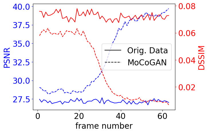
5.1 Datasets
Following the established evaluation protocol from previous studies [19, 29], we use the following benchmarks:
-
(1)
Human actions [3]: The dataset contains 81 videos of 9 people performing 9 actions, e.g. walking, jumping, etc. All videos are extracted with fps and down-scaled to pixels. We also add a flipped copy of each video sequence to the training set. Following Tulyakov et al. [29] we used only 4 action classes, which amounts to 72 videos for training in total.
-
(2)
UCF-101 [22]: This dataset consists of 13 220 videos with 101 classes of human actions grouped into 5 categories: human-object and human-human interaction, body motion, playing musical instruments, and sports. This dataset is challenging due to a high diversity of scenes, motion dynamics, and viewpoint changes.
-
(3)
Tai-Chi: The dataset contains 72 Tai Chi videos taken from the UCF-101 dataset.333Note that the Tai Chi subset used in the evaluation of MoCoGAN [29] is not publicly available and could not be obtained due to licensing restrictions. All videos are centered on the performer and downscaled to pixels. We use this dataset for our ablation studies as it has moderate complexity, yet represents real-world motion.
5.2 Overview
We first verify that t-PSNR and t-DSSIM effectively quantify the temporal artifacts. We then employ these metrics to analyze the MoCoGAN model [29] w.r.t. these artifacts. Next, we study the effect of the time-horizon hyperparameters, and , of our MDP approach. Finally, we validate our approach on the Human Actions dataset and on the more challenging UCF-101 dataset. We compare our model to TGAN [19] and MoCoGAN, where we find a consistent improvement of the temporal diversity over the baseline.
We compute the IS following Saito et al. [19], who trained the C3D network [28] on the Sports-1M dataset [10] and then further finetuned on UCF-101 [22]. For FVD we use the original implementation by Unterthiner et al. [30]. To manage computational time, we calculate the FVD for the first 16 frames, sampled from 256 videos, and derive the FVD mean and variance from 4 trials, similar to IS.
| Metric | Tai Chi | MoCoGAN | MDP model | ||||
| IS | 1.63 0.05 | 4.49 0.04 | 4.52 0.05 | 4.15 0.04 | 4.24 0.06 | 3.92 0.07 | 3.99 0.04 |
| FVD | 118 5 | 828 38 | 1108 50 | 787 10 | 782 40 | 744 40 | 809 22 |
| t-DSSIM | 0.0135 | 0.0031 | 0.0031 | 0.0024 | 0.0037 | 0.0035 | 0.0035 |
| t-PSNR | 36.48 | 45.37 | 57.34 | 50.16 | 44.87 | 44.39 | 45.06 |
5.3 Metric evaluation
We design a set of proof-of-concept experiments to study the properties of the newly introduced t-PSNR and t-DSSIM. Concretely, we synthesize the looping and freezing patterns in the ground-truth videos from UCF-101 and Tai Chi. We construct 16 frames by sampling 8 frames directly from the dataset and completing the sequence with an artifact counterpart. Looping-FWD contains a repeating subsequence from the original video (Original), whereas Looping-BWD reverses the frame order. The size of the re-occurring subsequence in Freezing is one. To put the results in context, we also compare to the mainstream IS as well as the recent FVD scores and study the robustness of all metrics to additive Gaussian noise . The results are summarized in Table 4.
We observe that t-PSNR and t-DSSIM correlate well with the more sophisticated IS and FVD. Recall that both IS and FVD require training a network on videos of fixed length, hence (i) can be computed only for short-length videos, due to GPU constraints; (ii) may be misleading (e.g. Tai Chi results in Table 4) when the training data for the inception network is different from the evaluated data. By contrast, t-PSNR and t-DSSIM prove to be faithful in quantifying the artifacts we study, as they are data-agnostic and accommodate videos of arbitrary length. However, our metrics are permutation invariant, do not assess the quality of the frames themselves, and are not robust to random noise. Hence we stress their complementary role to IS and FVD as a measure of the overall video quality.


5.4 MoCoGAN: a case study
Here, we study the temporal diversity of the MoCoGAN model [29] using our t-PSNR and t-DSSIM scores.
We train MoCoGAN444We use the publicly available code provided by the MoCoGAN authors at https://github.com/sergeytulyakov/mocogan. on the UCF-101 dataset with temporal windows of size , and apply our temporal metrics to the samples from the generator. To enable a more detailed view of the temporal dynamics, we inspect the video samples as a function of time in Fig. 4 by plotting the values of the summands in Eq. 8 for each timestep. To rule out the possibility of any degenerate phenomena in the original data, we also plot the corresponding curves of the ground-truth sequences alongside. This clearly shows that MoCoGAN exhibits a vanishing diversity of video frames – a pattern that is not found in the training data.
5.5 MDP approach: an ablation study
Here, we perform an ablation study of our MDP approach by varying the time-horizon hyperparameters, and , introduced in Sec. 3.2. Recall that controls the timespan of the future predictions modeled by the Q-value: lower values imply a shorter time horizon, whereas higher values encourage the model to learn long-term dependencies. Parameter , on the other hand, specifies how accounting for the long-term effect is distributed over the timesteps. High values specify equal distribution; lower values force the model to encode the long-term effects more in the earlier than in the later timesteps. As a boundary case, we also consider and to gage the effect of the architecture change in the video discriminator (TCN), which is needed to implement reward causality (c.f. Sec. 3.2). As quantitative measures, we use the Inception Score (IS) [20], the Fréchet Video Distance (FVD) [30], as well our temporal metrics, t-DSSIM and t-PSNR, introduced in Sec. 4.
The results in Table 1 show that by leveraging the increasing values of the time-horizon hyperparameters, our model clearly improves the temporal diversity in terms of t-PSNR and t-DSSIM. Moreover, we also observe that the TCN baseline (, ) performs worse than the original MoCoGAN in terms of temporal diversity. This is easily understood when considering that the TCN alone does not have any lookahead into the future (c.f. Fig. 2(b)). However, once we enable taking the future rewards into account by virtue of our MDP formulation, we not only reach but actually surpass the temporal diversity of the baseline MoCoGAN, as expected.
The somewhat inferior IS and FVD scores might be due to their sensitivity to the data prior, as discussed in Sec. 5.3. This hypothesis is also supported by a qualitative comparison between MoCoGAN and our MDP model. Figure 5 gives one such example; more results can be found in the supplemental material. While we observe no notable difference in per-frame quality, the motion between consecutive frames from our MDP model is more apparent than the samples from MoCoGAN (e.g., the torso of the performer).
| Model | K | Human Actions | UCF-101 | ||||||
| IS | FVD | t-DSSIM | t-PSNR | IS | FVD | t-DSSIM | t-PSNR | ||
| Raw dataset | – | 3.39 0.08 | 49 2 | 0.0815 | 23.35 | 40.80 0.26 | 452 49 | 0.0723 | 28.34 |
| TGAN (Normal) | 16 | 2.90 0.04 | 977 31 | – | – | 8.11 0.07 | 1686 24 | – | – |
| TGAN (SVC) | 16 | 3.65 0.10 | 227 10 | – | – | 11.91 0.21 | 1324 23 | – | – |
| MoCoGAN | 16 | 3.53 0.02 | 300 8 | 0.0259 | 33.76 | 11.15 0.10 | 1351 49 | 0.0337 | 33.29 |
| MoCoGAN- | 16 | 3.51 0.02 | 245 6 | 0.0243 | 34.79 | 11.48 0.15 | 1314 45 | 0.0358 | 33.61 |
| MoCoGAN | 24 | 3.47 0.02 | 318 9 | 0.0254 | 35.72 | 10.49 0.09 | 1352 49 | 0.0387 | 32.63 |
| MDP-0 (ours) | 16 | 3.55 0.03 | 1413 15 | 0.0559 | 33.31 | 6.16 0.08 | 2147 87 | 0.0160 | 47.36 |
| MDP (ours) | 16 | 3.55 0.02 | 641 8 | 0.0604 | 30.12 | 11.86 0.11 | 1277 56 | 0.0370 | 32.77 |
| MDP (ours) | 24 | 3.49 0.03 | 686 12 | 0.0661 | 29.39 | 12.14 0.18 | 1293 58 | 0.0454 | 31.05 |


5.6 Human Actions and UCF-101
We perform further experiments on the Human Actions and the more challenging UCF-101 datasets.555To ensure a fair comparison, we use the same inception network for IS and FVD and train other methods [19, 29] using the authors’ implementation (c.f. supplemental material for details). We select for our MDP model, which provide a good trade-off between the improved t-PSNR, t-DSSIM, FVD and only a slight drop of IS on Tai Chi (c.f. Sec. 5.2). For reference, we train the TCN baseline, MDP-0, by setting and to decouple the influence of modeling the long-term effects from the changes in the MoCoGAN architecture to comply with reward causality. We also train our MDP model and MoCoGAN on an extended temporal window . Recall that higher require more GPU memory, but give the model an advantage, since it observes longer sequences at training time. Therefore, we aim to mitigate the artifacts while keeping constant.
The quantitative results are summarized in Table 2. For both the Human Actions and UCF-101 datasets, we observe a consistent improvement of our MDP model in terms of temporal diversity measured by t-PSNR and t-DSSIM. Moreover, our model also outperforms MoCoGAN in terms of IS on both datasets, as well as FVD on the UCF-101 dataset. This can be explained by the more varied nature of motion on these datasets compared to the Tai Chi dataset, which makes taking into account future frames more important. On the Human Actions dataset, the FVD score for our model is inferior to MoCoGAN. Recall from Sec. 5.2, that for IS and FVD metrics we did not fine-tune the inception classifiers on the Human Actions dataset, which impedes the interpretability of the scores on this dataset. A visual inspection of the per-frame quality (c.f. Fig. 6 for examples) reveals no perceptual loss compared to the baseline model. In contrast, disabling MDP modeling (MDP-0) leads to a clear deterioration in video quality.


On both datasets, our model with is also superior to MoCoGAN with in terms of IS and FVD, and reaches on par performance in terms of t-PSNR and t-DSSIM. Yet, our MDP-based formulation is significantly more memory efficient, since extending the temporal window at training incurs addition memory costs. Concretely, at training time the MDP model with consumes roughly more memory than MoCoGAN, whereas setting for the original MoCoGAN incurs a higher memory footprint. Note that simply increasing the number of parameters of in MoCoGAN is less effective than our proposed MDP approach (see MoCoGAN- in Tab. 5.6). Also, our MDP model with improves further over on UCF-101 and regarding the temporal metrics on Human Actions. A visual inspection of the samples from Human Actions did not reveal any perceptible difference to MoCoGAN or our MDP with , despite the inferior IS and FVD scores; we believe this to be an artifact of the evaluation specifics. The IS score of our MDP model is slightly inferior only to TGAN [19]. However, TGAN can produce video sequences of only fixed length, whereas our MDP model can generate videos of arbitrary length, owing to the recurrent generator.
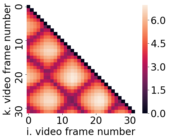
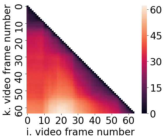
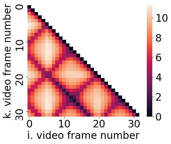
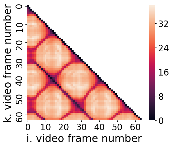
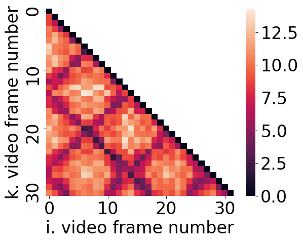
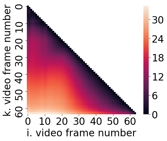
The qualitative results in Fig. 7 show that our model can generate complex scenes from UCF-101 that are visually comparable to the MoCoGAN samples. Similar to our observation on Human Actions, MDP-0 produces poorer samples, which asserts the efficacy of the underlying MDP. Since the interpretation of the UCF-101 results is difficult, we examine a visualization of a pairwise -distance between two frames in the video, shown in Fig. 8. The distance matrix can be represented as a lower triangular two-dimensional heatmap, owing to the symmetry of . We observe that while MoCoGAN exhibits a looping pattern, our MDP approach tends to preserve the temporal qualities of the ground-truth datasets. Note that some samples in Human Actions can be naturally periodic (e.g. hand-waving), hence, we do not expect our model to dispense with the looping pattern completely. The overall results suggest that modeling long-term dependencies with an MDP consistently leads to more diverse motion dynamics, which becomes more apparent in increasingly complex scenes.
 |
 |
 |
 |
 |
 |
6 Conclusions and Future Work
We revealed two pathological cases in the videos synthesized by the state-of-the-art MoCoGAN model, namely freezing and looping. To quantify the temporal diversity, we proposed an interpretable class of metrics. We showed that the SSIM- and PSNR-based metrics, t-PSNR and t-DSSIM, effectively complement IS and FVD to quantify temporal artifacts. Next, we traced the artifacts to the limited training length, which inhibits long-term modeling of the video sequences. As a remedy, we reformulated video generation as an MDP and incorporated it into MoCoGAN. We showed the efficacy of our MDP model on the challenging UCF-101 dataset both in terms of our temporal metrics, as well as in IS and FVD scores. Maintaining the recurrent state between the training iterations or imposing a tractable prior on the state suggest promising extensions of this work toward generating long-sequence videos.
Acknowledgements. The authors thank Sergey Tulyakov and Masaki Saito for helpful clarifications.
References
- [1] Mohammad Babaeizadeh, Chelsea Finn, Dumitru Erhan, Roy H. Campbell, and Sergey Levine. Stochastic variational video prediction. In ICLR, 2018.
- [2] Shaojie Bai, J. Zico Kolter, and Vladlen Koltun. An empirical evaluation of generic convolutional and recurrent networks for sequence modeling. arXiv:1803.01271 [cs.CV], 2018.
- [3] Moshe Blank, Lena Gorelick, Eli Shechtman, Michal Irani, and Ronen Basri. Actions as space-time shapes. In ICCV, 2005.
- [4] Chelsea Finn, Ian J. Goodfellow, and Sergey Levine. Unsupervised learning for physical interaction through video prediction. In NIPS*2016.
- [5] Ian Goodfellow, Jean Pouget-Abadie, Mehdi Mirza, Bing Xu, David Warde-Farley, Sherjil Ozair, Aaron Courville, and Yoshua Bengio. Generative adversarial nets. In NIPS*2014.
- [6] Jiawei He, Andreas M. Lehrmann, Joseph Marino, Greg Mori, and Leonid Sigal. Probabilistic video generation using holistic attribute control. In ECCV, 2018.
- [7] Martin Heusel, Hubert Ramsauer, Thomas Unterthiner, Bernhard Nessler, and Sepp Hochreiter. GANs trained by a two time-scale update rule converge to a local Nash equilibrium. In NIPS*2017.
- [8] Sepp Hochreiter and Jürgen Schmidhuber. Long short-term memory. Neural computation, 9(8):1735–1780, 1997.
- [9] Nal Kalchbrenner, Aäron van den Oord, Karen Simonyan, Ivo Danihelka, Oriol Vinyals, Alex Graves, and Koray Kavukcuoglu. Video pixel networks. In ICML, 2017.
- [10] Andrej Karpathy, George Toderici, Sanketh Shetty, Thomas Leung, Rahul Sukthankar, and Li Fei-Fei. Large-scale video classification with convolutional neural networks. In CVPR, 2014.
- [11] Diederik P. Kingma and Max Welling. Auto-encoding variational Bayes. In ICLR, 2014.
- [12] Bernhard Kratzwald, Zhiwu Huang, Danda Pani Paudel, Acharya Dinesh, and Luc Van Gool. Improving video generation for multi-functional applications. arXiv:1711.11453 [cs.CV], 2017.
- [13] Alex X. Lee, Richard Zhang, Frederik Ebert, Pieter Abbeel, Chelsea Finn, and Sergey Levine. Stochastic adversarial video prediction. arXiv:1804.01523 [cs.CV], 2018.
- [14] Xiaodan Liang, Lisa Lee, Wei Dai, and Eric P. Xing. Dual motion GAN for future-flow embedded video prediction. In ICCV, 2017.
- [15] Ziwei Liu, Raymond A. Yeh, Xiaoou Tang, Yiming Liu, and Aseem Agarwala. Video frame synthesis using deep voxel flow. In ICCV, 2017.
- [16] Michaël Mathieu, Camille Couprie, and Yann LeCun. Deep multi-scale video prediction beyond mean square error. In ICLR, 2016.
- [17] Katsunori Ohnishi, Shohei Yamamoto, Yoshitaka Ushiku, and Tatsuya Harada. Hierarchical video generation from orthogonal information: Optical flow and texture. In AAAI, 2018.
- [18] Marc’Aurelio Ranzato, Arthur Szlam, Joan Bruna, Michaël Mathieu, Ronan Collobert, and Sumit Chopra. Video (language) modeling: a baseline for generative models of natural videos. arXiv:1412.6604 [cs.LG], 2014.
- [19] Masaki Saito, Eiichi Matsumoto, and Shunta Saito. Temporal generative adversarial nets with singular value clipping. In ICCV, 2017.
- [20] Tim Salimans, Ian J. Goodfellow, Wojciech Zaremba, Vicki Cheung, Alec Radford, and Xi Chen. Improved techniques for training GANs. In NIPS*2016.
- [21] David Silver, Guy Lever, Nicolas Heess, Thomas Degris, Daan Wierstra, and Martin A. Riedmiller. Deterministic policy gradient algorithms. In ICML, 2014.
- [22] Khurram Soomro, Amir Roshan Zamir, and Mubarak Shah. UCF101: A dataset of 101 human actions classes from videos in the wild. arXiv:1212.0402 [cs.CV], 2012.
- [23] Nitish Srivastava, Elman Mansimov, and Ruslan Salakhutdinov. Unsupervised learning of video representations using LSTMs. In ICML, 2015.
- [24] Ilya Sutskever and Geoffrey E. Hinton. Learning multilevel distributed representations for high-dimensional sequences. In AISTATS, 2007.
- [25] Ilya Sutskever, Geoffrey E Hinton, and Graham W. Taylor. The recurrent temporal restricted Boltzmann machine. In NIPS*2009.
- [26] Richard S. Sutton and Andrew G. Barto. Introduction to Reinforcement Learning. MIT Press, 1998.
- [27] Graham W. Taylor, Geoffrey E Hinton, and Sam T. Roweis. Modeling human motion using binary latent variables. In NIPS*2017, 2007.
- [28] Du Tran, Lubomir Bourdev, Rob Fergus, Lorenzo Torresani, and Manohar Paluri. Learning spatiotemporal features with 3D convolutional networks. In ICCV, 2015.
- [29] Sergey Tulyakov, Ming-Yu Liu, Xiaodong Yang, and Jan Kautz. MoCoGAN: Decomposing motion and content for video generation. In CVPR, 2018.
- [30] Thomas Unterthiner, Sjoerd van Steenkiste, Karol Kurach, Raphaël Marinier, Marcin Michalski, and Sylvain Gelly. Towards accurate generative models of video: A new metric and challenges. arXiv:1812.01717 [cs.CV], 2018.
- [31] Aäron van den Oord, Nal Kalchbrenner, Lasse Espeholt, Koray Kavukcuoglu, Oriol Vinyals, and Alex Graves. Conditional image generation with PixelCNN decoders. In NIPS*2016.
- [32] Ruben Villegas, Jimei Yang, Seunghoon Hong, Xunyu Lin, and Honglak Lee. Decomposing motion and content for natural video sequence prediction. In ICLR, 2017.
- [33] Ruben Villegas, Jimei Yang, Yuliang Zou, Sungryull Sohn, Xunyu Lin, and Honglak Lee. Learning to generate long-term future via hierarchical prediction. In ICML, 2017.
- [34] Carl Vondrick, Hamed Pirsiavash, and Antonio Torralba. Generating videos with scene dynamics. In NIPS*2016.
- [35] Zhou Wang, Alan C. Bovik, Hamid R. Sheikh, and Eero P. Simoncelli. Image quality assessment: from error visibility to structural similarity. IEEE Trans. Image Processing, 13(4):600–612, 2004.
- [36] Tianfan Xue, Jiajun Wu, Katherine L. Bouman, and Bill Freeman. Visual dynamics: Probabilistic future frame synthesis via cross convolutional networks. In NIPS*2016.
Markov Decision Process for Video Generation
– Supplemental Material –
Vladyslav Yushchenko1∗ Nikita Araslanov2 Stefan Roth2
1iNTENCE automotive electronics GmbH, 2TU Darmstadt
Appendix A Overview
We elaborate on the evaluation protocol used in our study, as well as provide additional qualitative examples both from our approach and MoCoGAN \citesuppMoCoGAN. To enable reproducibility of our approach, we detail the architecture of our MDP-based video discriminator and the training specifics of our MDP approach.
Appendix B A Note on Reproducibility
In the main text, we indicated a discrepancy between the Inception Score (IS) we attained on UCF-101 \citesuppUCF-101 and the IS reported in the original work \citesuppTGAN, MoCoGAN. Recall that we compute the IS following Saito et al. \citesuppTGAN, who trained the C3D network \citesuppC3D on the Sports-1M dataset \citesuppSport1M and then further finetuned it on UCF-101 \citesuppUCF-101. We calculate the IS by sampling the first 16 frames from 10K videos and determining the mean and variance over 4 trials. As in previous work \citesuppTGAN, MoCoGAN, we use the first training split of the UCF-101 dataset.666More details on the splits of the UCF-101 dataset are available at http://crcv.ucf.edu/data/UCF101.php. We use original authors’ implementation, for both MoCoGAN777MoCoGAN repository provided at https://github.com/sergeytulyakov/mocogan. and TGAN888Code repository by \citesuppTGAN, provided at https://github.com/pfnet-research/tgan. and train the respective models for 100K iterations. We did not observe further improvements of the IS for longer training schedules.
To facilitate transparency and reproducibility of our experiments, we highlight two contributing factors that we carefully considered in our evaluation: IS implementation and model selection.
IS implementation. We found the IS to be sensitive to subtle differences in implementation. Recall that we use the original TGAN \citesuppTGAN evaluation code in our experiments. Algorithm-A in Fig. 9(a) shows the main steps of this evaluation for a single sample of video. While C3D \citesuppC3D is trained for a resolution of , video generators produce sequences of resolution . Additionally, C3D requires the input image sequence to be normalized with the mean and standard deviation used for the network training. The TGAN evaluation (c.f. Fig. 9(a)) upsamples the videos to , normalizes them, and feeds the center crop of into the C3D network. However, an alternative evaluation, shown by Algorithm-B in Figure 9(b), is to upsample the video directly to , applying the normalization at that scale, and feeding the result into C3D without cropping. This subtle change in the evaluation leads to a tangible difference in the Inception Score. We summarize the results in Table 11 and compare these two versions of evaluation to the reported scores in the original works \citesuppTGAN,MoCoGAN.
[1.15]
| Method | Inception Score | ||
| Reported | Reproduced Algorithm-A | Reproduced Algorithm-B | |
| MoCoGAN \citesuppMoCoGAN | 12.42 0.03 | 11.15 0.10 | 12.03 0.07 |
| TGAN-Normal \citesuppTGAN | 9.18 0.11 | 8.11 0.07 | 9.90 0.06 |
| TGAN-SVC \citesuppTGAN | 11.85 0.07 | 11.91 0.21 | 14.04 0.08 |
| MDP (ours) | 11.86 0.11 | 11.86 0.11 | 13.00 0.07 |
[0.9]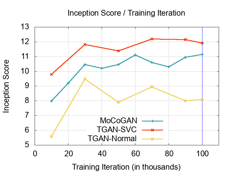
Leaving out cropping for IS computation with Algorithm-B leads to higher values of the IS in comparison to Algorithm-A. Note that the IS for MoCoGAN produced by Algorithm-B is closer to the reported values: it scores , which approaches the reported score of . However, the opposite is the case for TGAN-SVC as expected, since Algorithm-A is the unaltered version of the evaluation provided by the TGAN authors \citesuppTGAN (we attribute the discrepancy for TGAN-Normal to model selection, which we will discuss shortly). Importantly, regardless of the evaluation protocol our MDP model always outperforms the MoCoGAN baseline and achieves with Algorithm-B.
Although the choice of Algorithm-B over Algorithm-A does not change the ranking of the methods, we emphasize that mixing the results produced by the two algorithms does and can essentially invalidate the experimental conclusions. Therefore, we stick to Algorithm-A for all methods in the experiments that we presented in the main text.
We conclude that the specifics of IS implementation lead to tangibly different results and stress the importance of using the same evaluation strategy for all methods in the experiments. Moreover, we additionally report the Fréchet Video Distance (FVD) as well as our two new metrics, -PSNR and -DSSIM, in the main paper to provide a complementary view to the IS.
Model selection. Recall that the IS for TGAN-Normal using Algorithm-A, , is still inferior to the reported score of (c.f. Table 11). To investigate this discrepancy, we observe that the standard training objective \citesuppGAN used to train video generation models \citesuppTGAN,MoCoGAN serves only as a proxy criterion for the Inception Score. As a result, lower training loss, or even convergence of training, does not necessarily imply an improvement in the Inception Score. Figure 11 illustrates this observation: the Inception Score fluctuates over the course of training, even after a considerable number of training iterations. Indeed, the IS achieved by TGAN-Normal at around 30K iterations is the highest, , which is closer to the reported by the TGAN authors \citesuppTGAN (in fact better). Although it is disputable which strategy of selecting the final model for evaluation is more meaningful, we argue against searching for the best IS across training iterations. One reason is that there is no conventional train-test split for video generation, hence computing the IS for intermediate models amounts to “peeking” into the test-time performance of the model. Selecting the best IS also inhibits reproducibility. Since IS fluctuations are rather random, there can be no fixed training schedule defined a-priori to reproduce the result. Additionally, computing the IS is computationally expensive, as it requires thousands of forward passes with a pre-trained classification network (C3D).
We believe that more transparency both at the stage of model selection and IS implementation can improve reproducibility of the Inception Score. We adhere to this principle and ensure a pre-defined training schedule and exactly same evaluation methodology to enable a fair and reproducible experiments.
| Model | Conv3D | BatchNorm \citesuppBatchNorm | LeakyReLU \citesuppmaas2013rectifier | ||||
| Filters | Kernel | Stride | Padding | Dilation | |||
| 64 | 4,4,4 | 1,2,2 | 0,1,1 | 1,1,1 | ✓ | ✓ | |
| 128 | 4,4,4 | 1,2,2 | 0,1,1 | 1,1,1 | ✓ | ✓ | |
| 256 | 4,4,4 | 1,2,2 | 0,1,1 | 1,1,1 | ✓ | ✓ | |
| 1 | 4,4,4 | 1,2,2 | 0,1,1 | 1,1,1 | |||
| TCN | 64 | 3,4,4 | 1,2,2 | 2,1,1 | 1,1,1 | ✓ | ✓ |
| 128 | 3,4,4 | 1,2,2 | 4,1,1 | 2,1,1 | ✓ | ✓ | |
| 256 | 3,4,4 | 1,2,2 | 8,1,1 | 4,1,1 | ✓ | ✓ | |
| 1 | 1,4,4 | 1,2,2 | 0,1,1 | 1,1,1 | |||
Appendix C Additional Qualitative Examples
We make additional qualitative results available at https://sites.google.com/view/mdp-for-video-generation. The examples provide a visual comparison of MoCoGAN and our MDP-based model on the Tai Chi, Human Actions, and UCF-101 datasets.
Appendix D Implementation Details
D.1 Architecture
Recall that our MDP approach is based on an extension of the video discriminator from the original MoCoGAN model to a TCN-like model implementing reward causality. As Table 3 details, we only modify the temporal domain and replace the standard convolutions with their dilated variants. The hyperparameters of the TCN are the number of the dilated layers (blocks) and the convolution kernel size. Following Bai et al. \citesuppTCN, we set both hyperparameters to , since in such configuration the receptive field of the last TCN output covers the entire input sequence of frames. Note that the TCN version does not increase the number of parameters of the original , but even reduces it due to a smaller kernel size in the temporal domain. It is only the addition of the Q-value approximation that slightly increases the model capacity of . The architecture of the image discriminator and the generator remain in their original form \citesuppMoCoGAN.
D.2 Training details
We follow the training protocol of MoCoGAN \citesuppMoCoGAN and use the ADAM optimizer \citesuppADAM for training all networks with a learning rate of and moment hyperparameters , . As regularization, we only use weight decay of . We leave the settings for the motion and the content subspaces of MoCoGAN to their default parameters with and the motion dimension set to . We also keep the additive noise for images fed to the discriminators.
In order to be compatible with the MoCoGAN evaluation (c.f. Appendix B), all networks are trained for iterations with a mini-batch size of , while the seed is kept constant () to ensure equivalent parameter initialization across the experiments. For our ablation study on the Tai-Chi dataset, we used a batch size of and trained for iterations. The training length for the models is set to frames, unless explicitly stated otherwise. We sample the original data with a fixed sampling stride of , as in MoCoGAN training.999The documentation for training MoCoGAN is provided at https://github.com/sergeytulyakov/mocogan/wiki/Training-MoCoGAN. This means that in order to acquire frames for training, we extract a frame sequence with a random starting point from the ground truth dataset and take every second frame. This procedure increases the amount of motion by reducing the fps of the original video sequence, since e.g. on the UCF-101 dataset the originally sampled frames provide imperceptible changes to scene appearance.
ieee_fullname \bibliographysuppegbib_supp