Machine learning the thermodynamic arrow of time
Abstract
The mechanism by which thermodynamics sets the direction of time’s arrow has long fascinated scientists. Here, we show that a machine learning algorithm can learn to discern the direction of time’s arrow when provided with a system’s microscopic trajectory as input. The performance of our algorithm matches fundamental bounds predicted by nonequilibrium statistical mechanics. Examination of the algorithm’s decision-making process reveals that it discovers the underlying thermodynamic mechanism and the relevant physical observables. Our results indicate that machine learning techniques can be used to study systems out of equilibrium, and ultimately to uncover physical principles.
I Introduction
While the microscopic dynamics of physical systems are time reversible, the macroscopic world clearly does not share this symmetry. If we are shown a video of a macroscopic process, it is often easy to guess whether the movie is played in the correct or in time-reversed order, as in the latter case the observed sequence of events is utterly implausible. In 1927, Sir Arthur Eddington coined the phrase “time’s arrow” to express this asymmetry in the flow of events, arguing that it traces back to the second law of thermodynamics Eddington (1928).
In recent decades there has been increased interest in the out-of-equilibrium physics of microscopic systems, leading to a deepened understanding of non-equilibrium fluctuations and their relation to the second law Jarzynski (2011); Seifert (2012). In particular, it has become appreciated that fluctuations lead to an effective “blurring” of time’s arrow at the nanoscale, and that our ability to discern its direction can be quantified in a system-independent manner Feng and Crooks (2008); Jarzynski (2011); Hofmann et al. (2017).
Simultaneously, there have been significant advances in the ability of machine learning (ML) and artificial intelligence (AI) algorithms to tackle practical problems and to automate useful tasks. These include image and video classification Krizhevsky et al. (2012); Simonyan and Zisserman (2014); Szegedy et al. (2015); Karpathy et al. (2014); Pickup et al. (2014); Wei et al. (2018), medical diagnosis Esteva et al. (2017), playing games Silver et al. (2016), driving cars Buehler et al. (2009), and most recently analyzing scientific problems such as protein folding R.Evans et al. (2018). ML methods have also emerged as exciting tools to study problems in statistical and condensed matter physics, such as classifying phases of matter, detecting order parameters, and generating configurations of a system from observed data Torlai and Melko (2016); Carrasquilla and Melko (2017); van Nieuwenburg et al. (2017); Deng et al. (2017); Wetzel and Scherzer (2017); Wetzel (2017); Ch’ng et al. (2017, 2018); Liu and van Nieuwenburg (2018); Schindler et al. (2017a); Arsenault et al. (2014); Beach et al. (2018); van Nieuwenburg et al. (2018); Ponte and Melko (2017). These studies extend and further motivate the use of computer algorithms to learn physics from big data Schmidt and Lipson (2009); Rudy et al. (2017).
In the present work we ask whether a machine can learn to accurately guess the direction of time’s arrow from microscopic data, and if so, whether it does so by effectively discovering the underlying thermodynamics, identifying relevant quantities such as work and entropy production. We approach this problem within the framework of nonequilibrium statistical mechanics, numerically generating microscopic trajectories of irreversible physical processes. In many of the examples we consider, the system is small and the direction of time’s arrow is blurred, in the sense that both a given trajectory and its time-reversed image represent plausible sequences of events. In these cases the algorithm in principle cannot be perfectly accurate, and it becomes interesting to ask whether it is able to assess its own likelihood to guess the direction of time’s arrow correctly.
We find that the machine not only correctly classifies the direction of time’s arrow but also approximates the likelihood in the uncertain cases. Moreover, the machine can generate representative trajectories for forward and backward time directions correctly, i.e., it learns what a forward/backward trajectory should look like. We also design a neural network that can detect the underlying process and classify the direction of time’s arrow at the same time. Finally, we look inside the machine’s decision-making process and find that it correctly identifies dissipated work as the key quantity for optimally guessing the direction of time’s arrow.
We first introduce the relevant physical laws governing microscopic, non-equilibrium fluctuations. We then briefly review the ML techniques that we will use. Finally, we apply our methods to various model physical examples and we study the ability of ML techniques to learn and quantify the direction of time’s arrow.
II Thermodynamics and the arrow of time
When small systems undergo thermodynamic processes, fluctuations are non-negligible and the second law is expressed in terms of averages. Thus the Clausius inequality relating the work performed on a system to the net change in its free energy, , takes the form
| (1) |
where the angular bracket denotes an average over many repetitions of the process. Moreover, these non-equilibrium fluctuations satisfy strong constraints that allow us to rewrite such inequalities in terms of stronger equalities Jarzynski (1997a, b); Crooks (1998, 1999); Hummer and Szabo (2001), and to quantify the direction of time’s arrow as a problem in statistical inference Crooks (1998); Shirts et al. (2003); Maragakis et al. (2008); Feng and Crooks (2008); Jarzynski (2011). To frame this problem, let us first specify the class of processes we will study, and introduce notation.
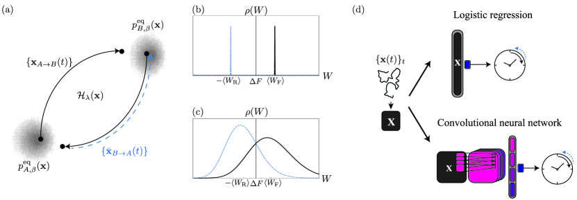
Consider a system in contact with a thermal reservoir at temperature . The system’s Hamiltonian depends on both the system’s microstate , and on an externally controllable parameter . An external agent performs work by manipulating this parameter. Now imagine that the system begins in equilibrium with the reservoir, and the agent then varies the parameter according to a schedule from to . We refer to this as the forward process. The trajectory describing the system’s evolution can be pictured as a movie, and is denoted by , where the time interval is implied. We also imagine the reverse process, in which the system starts in an equilibrium state at , and the agent varies the parameter from to according to . The trajectory (movie) for this process is denoted by . Finally, consider the time reversal of this trajectory, , where the ‘’ implies negation of momentum coordinates. This time-reversed trajectory corresponds to a movie of the reverse process, played backward in time; the same trajectory may have been achieved during a realization of the forward process, see Fig. 1(a).
Throughout this paper, we will use the term forward trajectory to refer to a trajectory generated during the forward process, i.e. , and we will use the term backward trajectory to denote a trajectory generated during the reverse process, but run backward in time, i.e. , depicted by the dashed blue line in Fig. 1(a).
Guessing the direction of time’s arrow can be cast as a game in which a player is shown either a forward or a backward trajectory – thus in either case the player “sees” the parameter being varied from to . The player must then guess which process, forward or reverse, was actually used to generate the trajectory Jarzynski (2006). The player’s score, or accuracy, is the ratio of correct predictions to the total number of samples.
In order to optimize the likelihood of guessing correctly, it suffices for the player to know the sign of the quantity , where is the work performed on the system and is the free energy difference between its initial and final states, as depicted in the movie. Specifically, let denote the likelihood that a given trajectory, , is obtained by performing the forward process, and let denote the likelihood that the trajectory is the time reversal of a realization of the reverse process. Note that . In addition, assume that the game is unbiased, e.g. the choice of performing the forward or reverse process in the first place was decided by flipping a fair coin. Then the likelihood that the trajectory was generated during the forward process is given by Shirts et al. (2003); Maragakis et al. (2008); Jarzynski (2011)
| (2) |
which is greater than (less than) 50% when is positive (negative). Here, the work performed by the external agent is
| (3) |
and the change in free energy is given by
| (4) |
where
| (5) |
is the partition function.
In macroscopic systems, the values of work performed on the system corresponding to forward trajectories, , and for backward trajectories, , are sharply peaked around their mean values, Fig. 1(b), and the sign of is a reliable indicator of the direction of time’s arrow. (Here, is the work performed during a given realization of the reverse process, therefore for the corresponding backward trajectory the work value is .) However, for microscopic systems these distributions can overlap significantly, as in Fig. 1(c). Eq. 2 shows that the player optimizes the chance of success simply by guessing “forward” whenever , and “reverse” otherwise, without accounting for any further details of the trajectory. Note that if then determining the arrow of time is easy, but when the problem becomes more difficult – in effect, time’s arrow is blurred.
III Neural networks
We wish to train a computer program to infer the direction of time’s arrow from a movie of the system’s trajectory. To do so, we first simulate a number of trajectories from the forward and the reverse processes, and we “time-reverse” the latter so that each trajectory is chronologically ordered with varying from to . We attach a label (reverse) or (forward) indicating which process was used to generate that trajectory. We then provide the machine with this collection of labelled trajectories, which will serve as the training data. A priori, any one of the trajectories could have been generated from either the forward or the reverse process, and the training stage now consists of using a neural network (NN) to construct a model of the function , which gives the likelihood the trajectory was generated by the forward process. Although this function is known analytically, Eq. 2, the machine is not provided with this information. We now sketch how the training is accomplished.
Since each (numerically generated) trajectory consists of a discretized time series of microstates, we represent the trajectory as a matrix whose rows correspond to different times, and whose columns correspond to phase space coordinates. The training stage amounts to designing a function that maps any such matrix onto a real number between 0 and 1, whose value is the machine’s best estimate of the likelihood that the trajectory was generated by the forward process.
In this work, we consider two types of classifiers: (i) logistic regression (LR), and (ii) convolutional neural network (CNN). The input to LR is a vectorized trajectory , and the output is , where is a vector of weights, is the bias, and is the logistic sigmoid function, see the top panel of Fig. 1(d). The CNN can compute more complicated functions than the LR Goodfellow et al. (2016). The input to our CNN is a trajectory matrix , and the output is again a value . The CNN has convolutional layers that extract useful information by taking advantage of the temporal and spatial structure of the data, see the bottom panel of Fig. 1(d). For details of the CNN architecture see Appendix A.
To train the network, we determine optimal values of parameters (such as the weights and biases in LR) by minimizing the cross-entropyGoodfellow et al. (2016)
| (6) |
Here the sum is carried over the training samples, is the label attached to the ’th trajectory, indicating which process was actually used to generate the trajectory, and is the output of the network for that trajectory.
Throughout this work, we always split a given data-set into three parts. We use 60%, 20% and 20% of the data for training, validation, and testing the model, respectively. The validation set is used to tune the architecture and hyperparameters of the model, while the test data is used for unbiased evaluation of the the final model’s accuracy. We use Adam optimizer with parameters suggested in the original paper for the training Kingma and Ba (2014). We assess the performance of the network by testing it over a balanced set of trajectories, i.e. half forward and half backward. If then the algorithm guesses that the trajectory was generated from the forward process, otherwise it guesses the reverse process. As a figure of merit, we consider the accuracy, i.e. the ratio of correct guesses to total number of samples. The best score that an algorithm can achieve, in the limit of a very large test set, is obtained if the output of the network agrees with the theoretical likelihood (2), in other words if the algorithm “learns” a result from nonequilibrium statistical physics.
For additional considerations in training NNs see Appendix A
IV Case studies
We apply the neural network machinery to detect the direction of the time’s arrow and assess the NN’s accuracy. We also look at the output of the network and compare it with the theoretical optimal result of Eq. (2). Interestingly, the networks not only learn to guess the direction of the time’s arrow but also learn to closely reproduce the likelihood function (see Appendix E for a discussion of the sensitivity of the results to the choice of the activation functions).
We first consider a single Brownian particle in a moving potential. This problem is simple and has an analytical solution.
We then move on to the more complicated problem of a spin chain with nearest-neighbour coupling in a magnetic field. We consider two scenarios involving the spin chain. First, the coupling is assumed to be constant, and the magnetic field is varied in time. Next, the magnetic field is constant the coupling is changed through time. We refer to the former as the B protocol, and the latter as the J protocol.
For details of the numerical calculations used to generate the trajectories see Appendix B. For details about the NNs and the number of samples used see Appendix A. Table 1 summarizes the accuracy of the algorithms studied in this and the following sections.
IV.1 Brownian particle in a moving potential
Consider an overdamped Brownian particle at temperature in a harmonic potential (see Fig. 2(a)), evolving according to
| (7) |
where denotes the strength of the potential, is the position of the center of the potential, and is the damping rate. The noise term, satisfies . In the forward protocol, the value of is changed from to at a fixed rate . Hence the reverse protocol changes from to with .
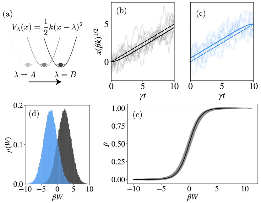
If the potential is moved rapidly, then in most of the forward trajectories the particle lags substantially behind the potential, whereas in most of the backward trajectories the particle leads the potential. In these cases, the direction of time’s arrow is clear. However, if the potential is moved slowly, then the particle stays near the center of the potential, the processes approach the reversible limit, and it becomes difficult to determine the direction of time’s arrow. The theoretical likelihood (2) is determined by the work performed and the free energy change, . Note that in this protocol . For each trajectory, we calculate by integrating
| (8) |
We generate samples of the forward and backward trajectories by numerically integrating the stochastic differential equation Eq. (7) (see Fig. 2(b) and (c)). We then train a classifier to predict the label for a given trajectory, as described earlier. In Fig. 2(e) we compare the accuracy and the output of a LR classifier (grey circles) with the theoretical likelihood (solid curve) obtained from Eqs. (8) and (2), see Table 1 and Fig. 2(e).
The seemingly remarkable agreement with the theory can be understood by examining (8). Namely, the work calculated by numerically integrating for a given trajectory is linearly related to the sum of the components of that vector. Therefore, LR is well-equipped to calculate this quantity and reproduce the likelihood function. See Appendix C.1 for detailed analysis of the optimal network.
IV.2 Spin chain - time-dependent field
Now let us consider a more complicated, many-particle system and a non-linear work protocol. Specifically, we consider a spin chain in a time-dependent magnetic field and in contact with a thermal reservoir at temperature , see Fig. 3(a), described by a Hamiltonian
| (9) |
where is the spin variable at site , and is the nearest-neighbour coupling strength. The dynamics of this system are modeled as a Markov process (See Appendix. B). The Hamiltonian aligns the spin in preferred energy configurations, while thermal fluctuations cause the spins to flip randomly according to a rate related to . We refer to this example as the protocol.
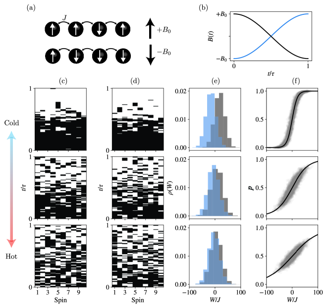
In the forward process, changes from a positive value at to a negative value at , as shown in Fig. 3(b). In the limit where , the spins start mostly aligned with the magnetic field. As the field magnitude is lowered, thermal fluctuations become dominant and the spins flip randomly. Eventually, becomes large and negative, and aligns the spin in the other direction (see the top row of Figs. 3 (c) and (d)). In this limit it is easy to detect the direction of the time’s arrow, as the work distributions have a modest overlap, see Fig. 3(e) top row. As the temperature is increased, thermal fluctuations increase the overlap in work distributions, blurring the direction of time’s arrow, see the middle and the bottom rows of Figs. 3(c), (d), and (e).
To train the classifier, we generate samples of forward and backward trajectories for three different temperatures using the Metropolis algorithm. The trajectories are matrices with entries, whose rows and columns correspond to time steps and spin positions, respectively. We are interested in training a single LR classifier that is capable of detecting the direction of time’s arrow for different temperatures. Therefore, the information about is provided through normalizing the elements of the trajectory data with their corresponding temperatures. This matrix is then reshaped as a vector to serve as the input to an LR classifier. We observe that the success of LR in learning both the correct labels and in approximating the likelihood function persists, see Table 1 and Fig. 3(f). The reason, again, lies in the functional form of , which can be evaluated by numerically integrating
| (10) |
It can be seen that is proportional to the weighted sum of the elements of the input vector. Note that, in this protocol . Consequently, LR is a perfect model of the likelihood function for all the temperatures, see Appendix C.1.
IV.3 Spin chain - time-dependent coupling
In this example, we consider a more complicated version of the spin chain problem, with a ferromagnetic-antiferromagnetic transition. Here, we keep constant and positive and allow for the time-dependent couplings , see Fig. 4(a). We refer to this example as the protocol. The Hamiltonian is given by
| (11) |
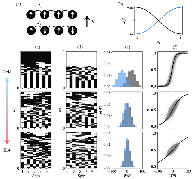
The protocol is shown in Fig. 4(b). In the forward case is varied from at to a at . Note that at low temperatures, where , the spins start in a state with anti-ferromagnetic ordering. As grows weaker during the protocol, thermal fluctuations dominate. By the end of the protocol, and the system settles in a state with ferromagnetic ordering. In this case, the forward and reverse work distributions are distinguishable, and so is the arrow of time, see the top rows of Fig. 4(c) - (e). As the temperature increases, so does the overlap between the distributions (the bottom two rows of Fig. 4(c) - (e)).
In this case the work is given by the time integral of
| (12) |
We see that is no longer linearly related to the input, and the LR classifier is incapable of calculating it. Therefore, we use a CNN with periodic boundary condition that can capture more complicated functions. With this CNN, we are able to recover the optimal accuracy again. Note that in this process , which adds another layer of complexity to the problem. The convolution layer in a CNN has filters that can capture the two-body nearest-neighbor correlations required to calculate the work, without introducing too many parameters. In fact, for a single temperature, we are able to analytically derive the parameters of a CNN that exactly calculate the likelihood function. The performance and the output of the network are shown in Table 1 and Fig. 4(f). For more details on the optimal network construction and the performance of sub-optimal strategies see Appendix C.3.
| Example | Accuracy (theory) | Accuracy (NN) |
|---|---|---|
| Brownian particle | ||
| Spin chain | ||
| Coarse-grained | ||
| Spin chain (LR) | ||
| Spin chain (CNN) | ||
| Coarse-grained | 89% | 88% |
V Interpretation and extensions
In this section, we use three approaches to investigate trained networks and to develop insight into what they have learned.
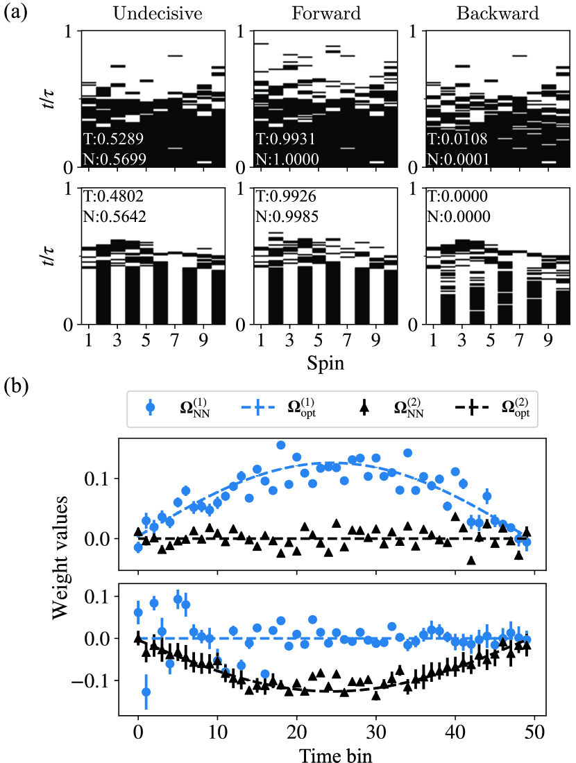
First, we use inceptionism techniques Mordvintsev et al. (2015); Schindler et al. (2017b) to learn the network’s ideal representative of forward and backward trajectories. Specifically, we use gradient descent on a random input such that the trained networks in Secs. IV.2 and IV.3 output 1 or 0 corresponding to forward and backward trajectories, respectively. This is in contrast with the previous section where we optimized for the weights and biases of the network. Among the simulated trajectories in the test set, we choose one with Schindler et al. (2017b) – this is a trajectory for which the classifier has difficulty assigning the direction of time’s arrow. We project the configurations to discrete values after each step of the gradient descent, and demand that there be at most 1 spin-flip per time step, to ensure that the network ‘dreams’ of physically realizable trajectories. We find that the networks’ ideas of the forward and backward trajectories show strong agreement with the true physical picture, see Fig. 5(a).
Secondly, to assign a physical interpretation to the networks’ decision-making process, we project the trajectories onto a two-dimensional reduced phase space corresponding to the collective coordinates and (taking period boundary conditions), representing magnetization and nearest-neighbour correlations, respectively. We also replace the value of within each time window of ten time steps, by the sum of the values within that window. By thus coarse-graining in both phase space and time, we reduce the noise due to finite size effects and variations over samples. Next, we use these coarse-grained trajectories to train LR classifiers for both protocols in Secs. IV.2 and IV.3 (See Table 1 for the performance of these networks). Finally, we investigate the weights that the networks assign to the magnetization () and the nearest neighbor correlations (). Fig. 5(b) reveals that for the B protocol (top row), the network mostly cares about the magnetization, whereas when the J protocol is performed (bottom row), the network bases its decision on the nearest-neighbor correlations. Moreover, the learned values of agree with our analytical results that reproduces the correct likelihood value (see Appendices C and D for details). These observations suggest that the network learns that the time derivative of the Hamiltonian, and by extension the work (3), is an important feature in guessing the direction of time’s arrow. We note that when the process is highly irreversible, the distributions of the forward and reverse work are well-separated. In this case, the network easily determines the arrow of time, but does not learn about the importance of work and bases its decision on other visible differences in the trajectories, see Appendix F.
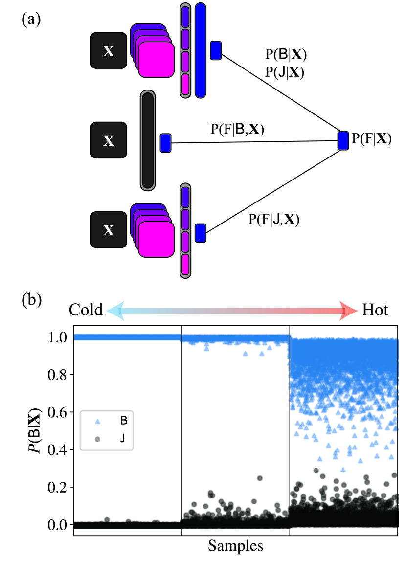
Lastly, we ask whether a single algorithm can learn to accurately guess the direction of time’s arrow for trajectories generated using multiple protocols, when the identity of the protocol is not specified. One approach is to take a large neural network and train it on trajectories from both and protocols. We have found that this approach works to a certain degree, but does not reach the accuracy of the individual networks in Secs. IV.2 and IV.3. However, by using our knowledge about the structure of the problem we can design an algorithm that attains the optimal performance. Specifically, we use a mixture of experts (MoE), with an output that is the weighted sum of expert networks Nowlan and Hinton (1990). When the protocol is not specified, the net forward likelihood is
| (13) |
The quantities and are modeled using neural networks similar to those considered in Secs. IV.2 and IV.3, respectively. These networks are referred to as experts. Additionally, we use a CNN to model . This CNN, which is called the gating network, learns the protocol from trajectories. Therefore, we obtain a larger three-headed network by combining the output of the three neural networks as in Eq. (13), as illustrated in Fig. 6(a). For the training, we use the pre-trained expert networks for the and protocols, and optimize the cost function (6) over sample trajectories from both protocols. We observe that the performance of this network is similar to that of the individual networks, as the gating network learns to accurately identify the protocol of input trajectories (see Fig. 6(b)). Note that the predictions of the gating network are more accurate at lower temperatures. This makes sense as the distribution of the initial state in the two protocols are distinguishable in low temperatures, but become less so as the temperature is increased.
VI Conclusion and outlook
Starting with a simple, solvable harmonic oscillator model, then proceeding to more complicated spin systems, we have shown that machine learning algorithms can be trained to discern the direction of time’s arrow in irreversible thermodynamic processes. We have found that neural networks not only learn to guess the direction of time’s arrow but also to accurately evaluate the likelihood that the guess is correct, when the direction of the arrow is not entirely clear. Moreover, we have used various techniques to interpret what the network learns. In particular, by examining the optimized parameter values that emerge from the training, we have been able to identify which physical quantities the network uses to guess the direction of time’s arrow. In this sense, our study represents a step toward AI driven discovery of physical concepts.
Machine learning techniques have been applied extensively to the study of equilibrium statistical physics Torlai and Melko (2016); Carrasquilla and Melko (2017); van Nieuwenburg et al. (2017); Wetzel (2017); Wetzel and Scherzer (2017); Ch’ng et al. (2017, 2018); Liu and van Nieuwenburg (2018); Schindler et al. (2017a); Beach et al. (2018); Ponte and Melko (2017). Our results extend this computational toolkit to out-of-equilibrium phenomena. While we have focused on the arrow of time, we expect that other important issues and questions in non-equilibrium physics can usefully be studied with these tools. We anticipate that the techniques considered in this work can be extended to estimate free energy differences, as well as to identify physical quantities that distinguish different regimes of dynamics in out-of-equilibrium quantum phenomena. In addition, using unsupervised learning techniques such as generative modeling may be especially useful in studying non-equilibrium phenomena Torlai and Melko (2016); Morningstar and Melko (2017). Unlike the equilibrium case where the state of the system is given by the Boltzmann distribution, the general form of the non-equilibrium steady-state is not known. Generative models are an ideal candidate to model and learn these distributions.
Moreover, machine learning researchers have shown that ML techniques can be used to detect the playback direction of real-world videos Pickup et al. (2014); Wei et al. (2018). These studies are concerned with videos of macroscopic objects that are in principle irreversible, and the arrow of time has a clear direction. In such scenarios, there are many indicators that can reveal the true playback direction, and therefore it is hard to quantify the optimal performance. However, in the physical examples the optimal attainable accuracy of the classifier is dictated by the laws of physics. Therefore, problems with large number of phase-space coordinates and with complicated dynamics, such as the J protocol for 2D Ising model, can serve as a standardized benchmark for video classification algorithms.
Acknowledgements
AS thanks Evert van Nieuwenburg, Grant Rostkoff, and Ali Izadi Rad for helpful discussions. AS and MH gratefully acknowledge support from ARO-MURI and Physics Frontier Center by National Science Foundation at the JQI and CJ from the National Science Foundation under grant DMR-1506969.
References
- Eddington (1928) A. S. Eddington, The nature of the physical world, (New York,The Macmillan Company, 1928) p. 392.
- Jarzynski (2011) C. Jarzynski, Annu. Rev. Condens. Matter Phys. 2, 329 (2011).
- Seifert (2012) U. Seifert, Reports on Progress in Physics 75, 126001 (2012).
- Feng and Crooks (2008) E. H. Feng and G. E. Crooks, Physical review letters 101, 090602 (2008).
- Hofmann et al. (2017) A. Hofmann, V. F. Maisi, J. Basset, C. Reichl, W. Wegscheider, T. Ihn, K. Ensslin, and C. Jarzynski, physica status solidi (b) 254, 1600546 (2017).
- Krizhevsky et al. (2012) A. Krizhevsky, I. Sutskever, and G. E. Hinton, in Advances in neural information processing systems (2012) pp. 1097–1105.
- Simonyan and Zisserman (2014) K. Simonyan and A. Zisserman, arXiv preprint arXiv:1409.1556 (2014).
- Szegedy et al. (2015) C. Szegedy, W. Liu, Y. Jia, P. Sermanet, S. Reed, D. Anguelov, D. Erhan, V. Vanhoucke, and A. Rabinovich, in Proceedings of the IEEE conference on computer vision and pattern recognition (2015) pp. 1–9.
- Karpathy et al. (2014) A. Karpathy, G. Toderici, S. Shetty, T. Leung, R. Sukthankar, and L. Fei-Fei, in CVPR (2014).
- Pickup et al. (2014) L. C. Pickup, Z. Pan, D. Wei, Y. Shih, C. Zhang, A. Zisserman, B. Scholkopf, and W. T. Freeman, in Proceedings of the IEEE Conference on Computer Vision and Pattern Recognition (2014) pp. 2035–2042.
- Wei et al. (2018) D. Wei, J. J. Lim, A. Zisserman, and W. T. Freeman, in Proceedings of the IEEE Conference on Computer Vision and Pattern Recognition (2018) pp. 8052–8060.
- Esteva et al. (2017) A. Esteva, B. Kuprel, R. A. Novoa, J. Ko, S. M. Swetter, H. M. Blau, and S. Thrun, Nature 542, 115 (2017).
- Silver et al. (2016) D. Silver, A. Huang, C. J. Maddison, A. Guez, L. Sifre, G. Van Den Driessche, J. Schrittwieser, I. Antonoglou, V. Panneershelvam, M. Lanctot, et al., Nature 529, 484 (2016).
- Buehler et al. (2009) M. Buehler, K. Iagnemma, and S. Singh, The DARPA urban challenge: autonomous vehicles in city traffic, Vol. 56 (springer, 2009).
- R.Evans et al. (2018) R.Evans, J.Jumper, J.Kirkpatrick, L.Sifre, T.F.G.Green, C.Qin, A.Zidek, A.Nelson, A.Bridgland, H.Penedones, S.Petersen, S. K.Simonyan, D.T.Jones, K. D.Silver, D.Hassabis, and A.W.Senior, Thirteenth Critical Assessment of Techniques for Protein Structure Prediction (Abstracts) (2018).
- Torlai and Melko (2016) G. Torlai and R. G. Melko, Phys. Rev. B 94, 165134 (2016).
- Carrasquilla and Melko (2017) J. Carrasquilla and R. G. Melko, Nature Physics 13, 431 (2017).
- van Nieuwenburg et al. (2017) E. P. van Nieuwenburg, Y.-H. Liu, and S. D. Huber, Nature Physics 13, 435 (2017).
- Deng et al. (2017) D.-L. Deng, X. Li, and S. Das Sarma, Phys. Rev. B 96, 195145 (2017).
- Wetzel and Scherzer (2017) S. J. Wetzel and M. Scherzer, Phys. Rev. B 96, 184410 (2017).
- Wetzel (2017) S. J. Wetzel, Physical Review E 96, 022140 (2017).
- Ch’ng et al. (2017) K. Ch’ng, J. Carrasquilla, R. G. Melko, and E. Khatami, Phys. Rev. X 7, 031038 (2017).
- Ch’ng et al. (2018) K. Ch’ng, N. Vazquez, and E. Khatami, Phys. Rev. E 97, 013306 (2018).
- Liu and van Nieuwenburg (2018) Y.-H. Liu and E. P. van Nieuwenburg, Physical review letters 120, 176401 (2018).
- Schindler et al. (2017a) F. Schindler, N. Regnault, and T. Neupert, Physical Review B 95, 245134 (2017a).
- Arsenault et al. (2014) L.-F. Arsenault, A. Lopez-Bezanilla, O. A. von Lilienfeld, and A. J. Millis, Physical Review B 90, 155136 (2014).
- Beach et al. (2018) M. J. Beach, A. Golubeva, and R. G. Melko, Physical Review B 97, 045207 (2018).
- van Nieuwenburg et al. (2018) E. van Nieuwenburg, E. Bairey, and G. Refael, Phys. Rev. B 98, 060301 (2018).
- Ponte and Melko (2017) P. Ponte and R. G. Melko, Phys. Rev. B 96, 205146 (2017).
- Schmidt and Lipson (2009) M. Schmidt and H. Lipson, Science 324, 81 (2009).
- Rudy et al. (2017) S. H. Rudy, S. L. Brunton, J. L. Proctor, and J. N. Kutz, Science Advances 3, e1602614 (2017).
- Jarzynski (1997a) C. Jarzynski, Physical Review Letters 78, 2690 (1997a).
- Jarzynski (1997b) C. Jarzynski, Physical Review E 56, 5018 (1997b).
- Crooks (1998) G. E. Crooks, Journal of Statistical Physics 90, 1481 (1998).
- Crooks (1999) G. E. Crooks, Physical Review E 60, 2721 (1999).
- Hummer and Szabo (2001) G. Hummer and A. Szabo, Proceedings of the National Academy of Sciences (USA) 98, 3658 (2001).
- Shirts et al. (2003) M. R. Shirts, E. Bair, G. Hooker, and V. S. Pande, Phys. Rev. Lett. 91, 140601 (2003).
- Maragakis et al. (2008) P. Maragakis, F. Ritort, C. Bustamante, M. Karplus, and G. E. Crooks, The Journal of chemical physics 129, 07B609 (2008).
- Jarzynski (2006) C. Jarzynski, Phys. Rev. E 73, 046105 (2006).
- Goodfellow et al. (2016) I. Goodfellow, Y. Bengio, and A. Courville, Deep Learning (MIT Press, 2016) http://www.deeplearningbook.org.
- Kingma and Ba (2014) D. P. Kingma and J. Ba, arXiv preprint arXiv:1412.6980 (2014).
- Mordvintsev et al. (2015) A. Mordvintsev, C. Olah, and M. Tyka, “Inceptionism: Going deeper into neural networks,” (2015).
- Schindler et al. (2017b) F. Schindler, N. Regnault, and T. Neupert, Phys. Rev. B 95, 245134 (2017b).
- Nowlan and Hinton (1990) S. J. Nowlan and G. E. Hinton, in NIPS (1990).
- Morningstar and Melko (2017) A. Morningstar and R. G. Melko, The Journal of Machine Learning Research 18, 5975 (2017).
- Srivastava et al. (2014) N. Srivastava, G. Hinton, A. Krizhevsky, I. Sutskever, and R. Salakhutdinov, The Journal of Machine Learning Research 15, 1929 (2014).
- Salinas (2001) S. R. A. Salinas, “The ising model,” in Introduction to Statistical Physics (Springer New York, New York, NY, 2001) pp. 257–276.
Appendix A Neural networks
A.1 Convolutions
A convolution layer convolves the input with a number of filters, and then applies a non-linear function to the output of the filters. Each convolution operation with a kernel and bias , maps an input matrix , to another matrix given by Goodfellow et al. (2016)
| (14) |
where specifies the number of steps the filter moves in each direction. It is called the stride of the convolution and is a hyperparameter that is tuned using the cross-validation data. The output of the convolution layer is obtained by applying a non-linear function element-wise to . The convolution layers can be repeated many times, and combined with pooling layers where the dimension of the output is reduced through a procedure such as averaging. At the end, the output of the convolution layer is flattened to form a vector and that vector is fed into a series of fully connected layers to produce the network’s output Goodfellow et al. (2016).
The CNN’s that we consider has four filters, with the stride of 1, and with periodic boundary condition. We choose the rectifier, i.e., , for the activation of these filters. The output of all the filters is then combined to form a single vector. For the CNN classifying the J protocol (Sec. IV.3), this vector is fed into a single neuron with sigmoid activation, whose values determine the direction of time’s arrow. For the gating network (Sec. V), this vector is fed into a fully connected layer with 50 hidden neurons and the rectifier activation, followed by the output neuron with the sigmoid activation.
A.2 Regularization and sample size
To reduce overfitting it is helpful to include a regularization term. This will help to reduce the difference between the training error and the test error. We consider regularization , that is adding the square of all the weights in the network to the cost function. The parameter is a hyper-parameter of the model and is tuned using the cross-validation data.
Additionally, in training the CNN in Sec. IV.3, we use the dropout technique to reduce overfitting. Dropout refers to deactivating and ignoring certain neurons during the training phase. Specifically, at every training step, a random fraction of of neurons are deactivated Srivastava et al. (2014).
We find that the performance of our algorithms does not vary significantly with the choice of hyper-parameters. We choose for the dropout rate of neurons of the convolutional layer in the J network, and for the gating network. The regularization rates are shown in Table 2.
| Model | |
|---|---|
| Brownian particle | |
| Spins | |
| Spins (LR) | |
| Spins (CNN all layers) | |
| Spins coarse-grained (all cases) | |
| Gating network (conv. and the hidden layer) | |
| Gating network (output) | |
| Alternative activation functions (all layers) |
Another important quantity in training the neural networks is the sample size. We use a total of 20000 samples for the Brownian particle. For the spin chain examples (B and J protocols), we use 20000 samples for each temperature. The samples are then split into three sets and are used to train, validate, and test the models.
Appendix B Generating the data
To generate trajectories we closely follow Ref. Crooks (1998). We consider a discrete set of time steps . The value of the control parameter and the state of the system at each time step is denoted by and , respectively. Note that in dealing with discrete time steps, rather than using , we use the notation for the value of variable at the time step . In the forward process, the initial state of the system is drawn from equilibrium with . The time evolution can be broken into two substeps:
-
(i)
With the state of the system fixed, the control parameter is changed
-
(ii)
At fixed , the state of the system evolves
Here, the second substep is either generated by a stochastic differential equations (Sec. IV.1) or Metropolis algorithm (Secs. IV.2 IV.3). The total work performed in this process is
| (15) |
For producing backward trajectories, the system is initialized in an equilibrium state with . The dynamics begin with a change in the system state, followed by a change in . In the end, the history of the system state is reversed, and the calculated work is negated to obtain backward trajectories and their corresponding work values.
Appendix C Optimal networks
For some of the examples that we considered, it is possible to derive an analytical expression for the optimal weights and biases of the network. Specifically, we examine the expression that is used to calculate the work and the change in free energy . Because the logistic sigmoid activation function, i.e., , used for classification coincides with the form of the likelihood function (2) in the arrow of time problem, we are able to find the networks parameters that reproduce the same likelihood function. To illustrate, consider the LR model with the output and . If we find and such that , the output of the network correctly represent . In the following we show that when (15), is linear in the elements of and is subsequently linear in elements of , we are able to find such optimal and .
C.1 Brownian particle in a moving potential
In this example, the system’s state at each time step is described by a scalar , i.e. the position of the particle. We have a total of time steps, therefore the input to the NN is a dimensional vector. The LR classifier considered here, is parameterized by a dimensional weight vector with elements for and a bias . Using Eq. (15) we find
| (16) |
where is independent of , because the protocol is linear. Note that in this example. With the choice of
| (17) | ||||
| (18) |
we can see that , where .
C.2 Spin chain - B protocol
The full trajectory of an spin system over time steps is represented by a matrix . We denote the orientation (up or down) of the th spin at time with . The input to LR classifier, is a vector obtained from rearranging the trajectory matrix to shape it into an array. By using Eq. (15) we find that
| (19) |
where . Work calculated using Eq. (19) is the discrete time version of obtained from Eq. (10). In this example, again, and we find that the optimal weights and bias are given by
| (20) | ||||
| (21) |
where . Note that if the input is scaled with , a single LR classifier is able to reproduce the correct likelihood for different temperatures.
C.3 Spin chain - J protocol
Using the same notation in the previous section, we find that the work, , is given by
| (22) |
where . Work calculated using Eq. (22) is the discrete time version of obtained from Eq. (12). We also use periodic boundary condition, which implies . Moreover, there is a non-zero change in the free energy, which is given by Salinas (2001)
| (23) |
where
| (24) |
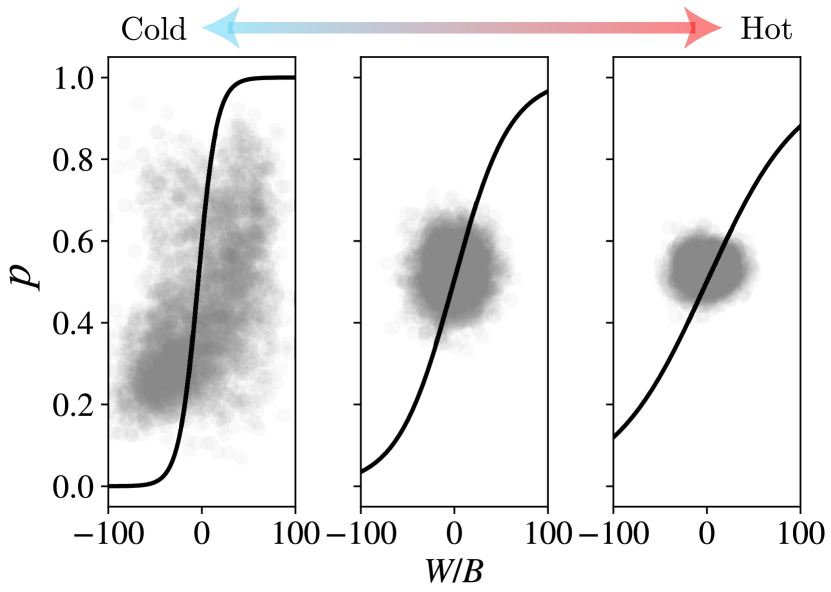
We see that it is not possible to have a logistic regression model that calculates (see Fig. 7).
However, CNN’s can, in principle, learn the relevant representation (i.e. nearest-neighbor correlations) from the input data, and learn the corresponding weights to calculate work. Specifically, to show that in principle a CNN can exactly calculate the correct likelihood from the input, we consider a CNN with four filters with periodic boundary condition and the rectifier activation , followed by the output layer with sigmoid activation . We set the biases of the convolutional layer to zero, and choose the weights for filters as follows
| (25) |
Each filter is only activated for one of the possible configuration of two neighboring spins. Specifically, given the input , the output of each filter is a matrix such that
| (26) | ||||
| (27) | ||||
| (28) | ||||
| (29) |
and otherwise. We can now rewrite the output of the network as
| (30) |
where contains the weights of the output layer corresponding to . The optimal values of these weights are given by
| (31) | ||||
| (32) | ||||
| (33) |
where .
Therefore, a CNN with four filters is sufficient to capture the likelihood at a single temperature of . We find that in practice, a CNN with such an architecture is likely to get stuck at local minima, and finding the optimal parameters shown above greatly depends on the initial weights of the network. However, we observe that a CNN with four filters can achieve a close to optimal performance more easily.
Appendix D Coarse-grained features
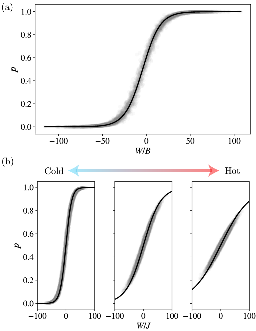
To reduce the parameters of the neural network and simplify the task of learning we pre-calculate a set of features for the network. Specifically, for the two protocols concerning the spin chain in a magnetic field, the coarse-grained features are
| (34) | ||||
| (35) |
where is an integer and is the scaled time. Using this feature map, LR classifier can calculate for both B and J protocols (See Fig. 8). The input to the network is a dimensional vector . We denote the weights corresponding to by dimensional vectors for . In this case, we approximate the optimal weights and bias of the networks by their average over the coarse-grained time window. For the B protocol we find
| (36) | ||||
| (37) | ||||
| (38) |
Similarly, the weights and bias for the J protocol are given by
| (39) | ||||
| (40) | ||||
| (41) |
In both cases we can see that , where the approximation comes from coarse-graining.
Note that in this case, even though LR classifier can calculate if the input is scaled with , it is not possible to train the network over different temperatures. This is because , and a simple bias cannot capture multiple values of . Therefore, we only consider a single temperature for the J protocol in studying the optimal networks with coarse-grained features.
Appendix E Alternative activation functions
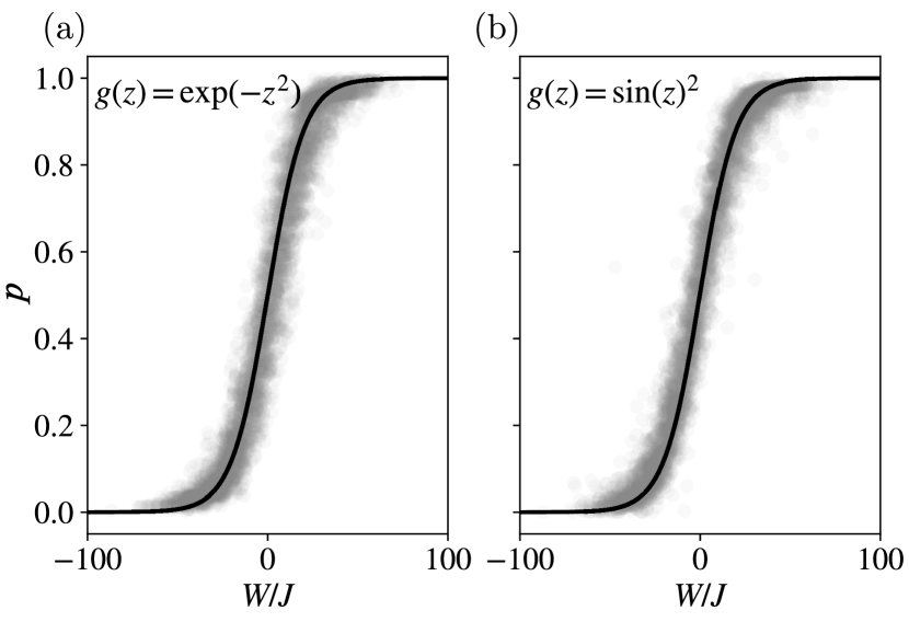
The logistic function that appears in the theoretically calculated likelihood in the time’s arrow problem, is similar to the activation function that is commonly used for classification in machine learning. To assess the general ability of the networks in approximating the likelihoods we try different activation functions. Specifically, we choose and as the activation of the last layer of the neural network so that the output is always between 0 and 1, and can be interpreted as probabilities. We also add a hidden layer to give the network the ability to calculate complex functions. We compare the network’s output with the theoretical likelihoods for the spin chain under the B protocol with coarse-grained feature discussed in Sec. D. We only train the network at a single temperature and observe that the network can still approximate the likelihood function as shown in Fig. 9.
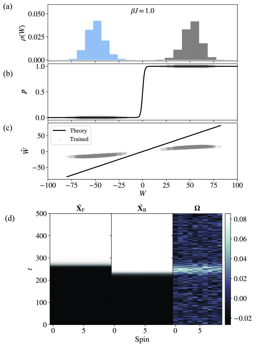
Appendix F Highly irreversible processes
When the process is highly irreversible, the arrow of time has a clear direction. In such cases, we observe that while LR has 100% accuracy, it does not learn work (obtained by inverting the sigmoid function in the output). This is because, the events that enable the network to learn work are extremely rare, and are usually absent in the training data. However, there are other evident differences that can show the direction of time’s arrow. We show an example of such a process for the B protocol at low temperatures. We observe that the orientation of spins undergoes a sharp transition as the magnetic field changes sign. However, the time that this transition occurs is different in the forward and backward trajectories. The classifier makes a decision based on the spin configuration at this particular time.
