Stability dependence of local structural heterogeneities of stable amorphous solids

Abstract

The universal anomalous vibrational and thermal properties of amorphous solids are believed to be related to the local variations of the elasticity. Recently it has been shown that the vibrational properties are sensitive to the glass’s stability. Here we study the stability dependence of the local elastic constants of a simulated glass former over a broad range of stabilities, from a poorly annealed glass to a glass whose stability is comparable to laboratory exceptionally stable vapor deposited glasses. We show that with increasing stability the glass becomes more uniform as evidenced by a smaller variance of local elastic constants. We find that, according to the definition of local elastic moduli used in this work, the local elastic moduli are not spatially correlated.

I Introduction

The vibrational modes and the low temperature thermal properties of amorphous solids are sharply different from those of their crystalline counterparts Zeller and Pohl (1971); Stephens (1973); Zaitlin and Anderson (1975); Pohl et al. (2002). The uniform structure of crystals allows for the description of the low frequency modes as if it were a classical elastic body whose properties are governed by the elastic moduli, which forms the basis of the Debye model for the density of states. This description leads to a $T^{3}$ increase of the specific heat for crystalline solids due to the increase of the density of the vibrational modes as the square of the frequency $\omega$. Recently it was shown that the low frequency vibrational modes of amorphous solids can be divided into a Debye term and an excess contribution that increases as the fourth power of the frequency Mizuno et al. (2017); Wang et al. (2019). The excess modes are spatially quasi-localized. Their spatial extent and density decrease with increasing stability. The quasi-localized character of excess modes suggests that there might be a spatially varying local elasticity.

Indeed, there is a large body of evidence for the existence of spatially varying local elastic constants in amorphous solids Mizuno et al. (2013, 2016); Yoshimoto et al. (2004); Tsamados et al. (2009); Léonforte et al. (2006); Mizuno et al. (2014); Gelin et al. (2016); Caroli and Lemaître (2019); Fan et al. (2014); Mizuno et al. (2013); Wagner et al. (2011); Mizuno et al. (2016); Pogna et al. (2019). To explain a plateau observed in the thermal conductivity around 10K for many dielectric amorphous solids, a Rayleigh like scattering of sound waves was assumed Zeller and Pohl (1971); Pohl et al. (2002). This assumption posits scattering from uncorrelated defects that are much smaller than the wavelength of the sound wave, and these defects would naturally give rise to local variations of the elasticity. Further theoretical analysis assuming local variations of the elasticity reproduces the $\omega^{4}$ excess in the vibrational density of states and predicts the Rayleigh scaling $k^{4}$ (where $k$ is a wavevector) of sound attenuation Schirmacher et al. (2007, 2010); Mizuno and Ikeda (2018); Wang et al. (2019). The $k^{4}$ scaling of sound attenuation was questioned in a computer simulation study Gelin et al. (2016) and a logarithmic correction to the Rayleigh scaling was proposed. This correction was rationalized in terms of a power law decay of the spatial correlations of the local elasticity. However, other simulation studies Mizuno and Ikeda (2018); Wang et al. (2019); Moriel et al. (2019) suggest that the logarithmic correction either exists only for a narrow range of wavevectors (frequencies) or this correction is only a good description of the crossover region between the high and low wavevector (frequency) behavior of sound attenuation.

Pogna et al. Pogna et al. (2019) examined sound attenuation in geologically hyperaged, ultrastable amber within the framework of fluctuating elasticity theory to establish a link between stability and the local variation of the elastic constants. They fitted the predictions of the theory for the vibrational density of states to the experimental data and in this way obtained estimates of the relative variance of the local elastic constants and of a length scale characterizing their spatial variation. They concluded that there was a reduction in the variation of the elastic constants by around 6% and an increase of the characteristic length scale of around 22% in the hyperaged amber compared to a liquid cooled sample. Thus, increasing stability seemingly narrows the distribution of elastic constants and increases the range of their correlations.

However, in a very recent simulational study Caroli and LemaitreCaroli and Lemaître (2019) argued that the fluctuating elasticity theory does not describe well sound attenuation in amorphous solids. They based this conclusion on two results. First, they showed that the fluctuating elasticity theory predicts the $k^{4}$ Rayleigh scattering-like sound damping whereas their simulations were consistent with a logarithmic correction. Second, they measured the parameters that enter into the fluctuating elasticity theory in simulations, used them to calculate sound attenuation, and compared these predictions with sound attenuation observed in the same simulations. They found that the predicted sound attenuation is two orders of magnitude smaller than the observed one. The second fact implies that the fluctuating elasticity theory severely underestimates the magnitude of the sound attenuation even if one were to argue that the logarithmic corrections is an intermediate, finite wavevector feature and the sound attenuation can be described within the Rayleigh scattering picture.

We note that it is difficult to directly probe local variations of the elasticity in experiments Wagner et al. (2011), which forced Pogna et al. to treat the relative variance of the local shear modulus as a fitting parameter. In contrast, simulations are able to calculate local elastic constant using several different methods Gelin et al. (2016); Mizuno and Ikeda (2018); Mizuno et al. (2013). Using one of these methods, Mizuno, Mossa, and Barrat found that the width of the distribution of local elastic constant correlates with sound attenuation Mizuno et al. (2014). For their study, they continuously transformed a crystal into an amorphous solid by continuously changing the size ratio of a binary mixture. Using the same technique they also demonstrated that the thermal conductivity, the lifetime of acoustic modes, and the local elastic heterogeneity are correlated Mizuno et al. (2016). This investigation, however, does not mimic the experimental procedure of Pogna et al.Pogna et al. (2019) who studied the stability dependence of sound attenuation. Importantly, in the work of Mizuno, Mossa, and Barrat the system is changed systematically in order to establish the correlations between the transport and acoustic properties and the variation of local elastic constants.

Here we examine the dependence of local elastic moduli of a simulated polydisperse glass former on its stability. We partition the system into different box sizes $w$ and determine the distribution of local elastic moduli for three values of $w$. We find that the width of the distribution decreases with increasing stability. However, using our definition of the local elastic moduli, we find that the local elastic moduli are uncorrelated in space.

II Methods

II.1 Molecular Dynamics Simulations

We studied a system of $N=48000$ and $N=192000$ polydisperse repulsive particles in a cubic box of volume $V$ with periodic boundaries in 3D. The pair potential is given by

$$U(r_{ij})=\begin{cases}\epsilon\left(\frac{\sigma_{ij}}{r_{ij}}\right)^{12}+v(r_{ij}),\hskip 20.0pt&\frac{\sigma_{ij}}{r_{ij}}<r_{\text{cut}}\\[10.0pt] 0,\hskip 20.0pt&\frac{\sigma_{ij}}{r_{ij}}\geq r_{\text{cut}}\end{cases}$$ (1)

with

$$v(r_{ij})=c_{0}+c_{2}\left(\frac{r_{ij}}{\sigma_{ij}}\right)^{2}+c_{4}\left(\frac{r_{ij}}{\sigma_{ij}}\right)^{4}.$$ (2)

The distance between particle $i$ and particle $j$ is $r_{ij}=|$r${}_{i}-$r${}_{j}|$, $\sigma_{ij}=\frac{\sigma_{i}+\sigma_{j}}{2}\left(1-0.2|\sigma_{i}-\sigma_{j}|\right)$Wang et al. (2019); Ninarello et al. (2017). The size of an individual particles $\sigma$ are given by the probability distribution

$$P(\sigma)=\frac{A}{\sigma^{3}}$$ (3)

where $\sigma\in[0.73,1.63]$ and zero otherwise. The coefficients $c_{0}$, $c_{2}$, and $c_{4}$ are chosen to guarantee the continuity of the potential up to the second derivative at the cutoff distance $r_{\text{cut}}=1.25$. This choice of system and polydispersity inhibits crystallization and fractionation while allowing the swap Monte Carlo algorithm to equilibrate to low temperatures Ninarello et al. (2017). We present the results in reduced units with $\epsilon$ being our unit of energy, the average of $\sigma=\sigma_{0}$ being our unit of length, and $\sqrt{m\sigma_{0}^{2}/\epsilon}$ being the unit of time.

For each parent temperature $T_{\text{p}}\in[0.062,0.200]$ we studied 4 independent initial configurations at number density $\rho=1$. Each configuration was first equilibrated at its parent temperature and then quenched to an inherent structure via the conjugate gradient algorithm. For reference, for our system the mode-coupling temperature $T_{\text{MCT}}\approx 0.108$ and the glass transition temperature $T_{g}\approx 0.072$ Ninarello et al. (2017). The equilibration was done using the swap Monte Carlo algorithm that combines conventional Monte Carlo moves with particle swaps Grigera and Parisi (2001); Gutiérrez et al. (2015); Ninarello et al. (2017).

After quenching, we ran very low temperature NVT molecular dynamics simulations using LAMMPS lam ; Plimpton (1995) code to which we added the interaction potential for the present model. The time step for all of MD simulations was $dt=0.02$. We first ran short equilibration runs at $T=10^{-5}$ in an NVT ensemble using a Nosé-Hoover thermostat. We then ran NVT production runs. Their length was determined by the time needed for to decorrelate a term involving the local and global stress $\left\langle\sigma_{\alpha\beta}^{m}\sigma_{\gamma\delta}\right\rangle$, which was identified as a slowly decorrelating term and discussed by Mizuno et al. Mizuno et al. (2013) and is defined in Section II.2. We found that there were no finite size effects, but, consistently with the observation made in Ref. [Mizuno et al. (2013)], much longer production runs are needed for larger systems. For a system of $N=48000$ particles, which is mainly used to perform the elastic modulus calculations in this study, the length of the production runs time was $\Delta t=3\times 10^{5}$, which corresponds to $1.5\times 10^{7}$ time steps. The results shown in the paper are for the $N=48000$ particle system unless otherwise specified. We observed very infrequent jumps in the energy and the pressure even at the very low temperature that we used, $T=10^{-5}$. We attribute these jumps to transitions between the locally stable minima. In the analysis we only use a continuous portion of the trajectory that excludes the energy jumps.

II.2 Elastic Modulus Calculations

To measure the local elastic response, the system is equally partitioned into cells of size $w=3.30$, $4.54$, $6.05$, and $12.11$. Several methods have been proposed to define and calculate the local elastic constants. Here we use the so-called “fully local” approach described by Mizuno, Mossa, and Barrat Mizuno et al. (2013). This approach was also used in other studies Mizuno et al. (2016, 2014, 2013). For each box $m$ the volume averaged stress tensor is calculated as:

$$\sigma_{\alpha\beta}^{m}=-\rho^{m}T\delta_{\alpha\beta}+\frac{1}{w^{3}}\sum_{i<j}\frac{\partial U(r^{ij})}{\partial r^{ij}}\frac{r_{\alpha}^{ij}r_{\beta}^{ij}}{r^{ij}}\frac{q^{ij}_{m}}{r^{ij}}$$ (4)

where, $\rho^{m}$ is the local number density of cell $m$, $T$ is the temperature, $\delta$ is the Kronecker delta and $r_{ij}=|\mathbf{r}_{i}-\mathbf{r}_{j}|$. The parameter $q^{ij}_{m}$ is the segment of the line joining $\mathbf{r}_{i}$ and $\mathbf{r}_{j}$ that lies within the box $m$. We use Greek subscripts to denote the Cartesian coordinates ($\alpha,\beta,\gamma,\delta=x,y,z$) and Roman superscripts to denote particle labels. The global stress tensor is given by:

$$\sigma_{\alpha\beta}=\frac{1}{V}\sum_{m}w^{3}\sigma_{\alpha\beta}^{m}=-\hat{\rho}T\delta_{\alpha\beta}+\frac{1}{V}\sum_{i<j}\frac{\partial U(r^{ij})}{\partial r^{ij}}\frac{r_{\alpha}^{ij}r_{\beta}^{ij}}{r^{ij}}.$$ (5)

We first calculate the local modulus $C_{\alpha\beta\gamma\delta}^{m}$ given by

$$C_{\alpha\beta\gamma\delta}^{m} = C_{\alpha\beta\gamma\delta}^{Am}-C_{\alpha\beta\gamma\delta}^{Nm}$$

$$= C_{\alpha\beta\gamma\delta}^{Bm}+C_{\alpha\beta\gamma\delta}^{Cm}+C_{\alpha\beta\gamma\delta}^{Km}-C_{\alpha\beta\gamma\delta}^{Nm}$$

$$C_{\alpha\beta\gamma\delta}^{Bm} = \frac{1}{w^{3}}\left\langle\sum_{i<j}\left(\frac{\partial^{2}U}{\partial r^{ij^{2}}}-\frac{1}{r^{ij}}\frac{\partial U}{\partial r^{ij}}\right)\frac{r^{ij}_{\alpha}r^{ij}_{\beta}r^{ij}_{\gamma}r^{ij}_{\delta}}{r^{ij^{2}}}\frac{q^{ij}_{m}}{r^{ij}}\right\rangle$$

$$C_{\alpha\beta\gamma\delta}^{Cm} = -\frac{1}{2}\Big{[}2\left\langle\sigma_{\alpha\beta}^{m}\right\rangle\delta_{\gamma\delta}-\left\langle\sigma_{\alpha\gamma}^{m}\right\rangle\delta_{\beta\delta}$$

$$-\left\langle\sigma_{\alpha\delta}^{m}\right\rangle\delta_{\beta\gamma}-\left\langle\sigma_{\beta\gamma}^{m}\right\rangle\delta_{\alpha\delta}-\left\langle\sigma_{\beta\delta}^{m}\right\rangle\delta_{\alpha\gamma}\Big{]}$$

$$C_{\alpha\beta\gamma\delta}^{Km} = 2\left\langle\hat{\rho}^{m}\right\rangle T\left(\delta_{\alpha\gamma}\delta_{\beta\delta}+\delta_{\alpha\delta}\delta_{\beta\gamma}\right)$$

$$C_{\alpha\beta\gamma\delta}^{Nm} = \frac{V}{T}\left(\left\langle\sigma_{\alpha\beta}^{m}\sigma_{\gamma\delta}\right\rangle-\left\langle\sigma_{\alpha\beta}^{m}\right\rangle\left\langle\sigma_{\gamma\delta}\right\rangle\right),$$ (6)

where $C_{\alpha\beta\gamma\delta}^{Am}$ is the affine contribution and $C_{\alpha\beta\gamma\delta}^{Nm}$ is the non-affine contribution. While the non-affine contribution vanishes in perfect crystalline systems at zero temperature, it has a magnitude comparable to the affine term in amorphous systemsTanguy et al. (2002). The brackets $\left\langle\cdots\right\rangle$ denotes an ensemble average. The Born contribution $C_{\alpha\beta\gamma\delta}^{Bm}$ to the affine term stems from the uniform displacement of all particles and it determines the instantaneous elastic modulus under such displacementsYoshimoto et al. (2004). The $C_{\alpha\beta\gamma\delta}^{Cm}$ term is due to the initial stress having a finite value Mizuno et al. (2013). The $C_{\alpha\beta\gamma\delta}^{Km}$ term is the kinetic energy contribution to the local elastic modulus tensor. Compared to the Born and the non-affine terms, the kinetic energy contribution to the elastic constant is negligible.

As described by Mizuno et al. Mizuno et al. (2013), the local bulk modulus $K^{m}$ is defined from the pressure-volume change and the five shear moduli $G^{m}_{1}$, $\cdots$, $G^{m}_{5}$, are defined from two pure shear and three simple shear deformations. These moduli are given by the following linear combinations of $C_{\alpha\beta\gamma\delta}^{m}$

$$K^{m} = \left(C^{m}_{xxxx}+C^{m}_{yyyy}+C^{m}_{zzzz}+C^{m}_{xxyy}\right.$$

$$\left.+C^{m}_{yyxx}+C^{m}_{xxzz}+C^{m}_{zzxx}+C^{m}_{yyzz}+C^{m}_{zzyy}\right)/9$$

$$G^{m}_{1} = \left(C^{m}_{xxxx}+C^{m}_{yyyy}-C^{m}_{xxyy}-C^{m}_{yyxx}\right)/4$$

$$G^{m}_{2} = \left[C^{m}_{xxxx}+C^{m}_{yyyy}+4C^{m}_{zzzz}+C^{m}_{xxyy}+C^{m}_{yyxx}\right.$$

$$\left.-2\left(C^{m}_{xxzz}+C^{m}_{zzxx}+C^{m}_{yyzz}+C^{m}_{zzyy}\right)\right]/12$$

$$G^{m}_{3} = C^{m}_{xyxy}$$

$$G^{m}_{4} = C^{m}_{xzxz}$$

$$G^{m}_{5} = C^{m}_{yzyz}.$$ (7)

The moduli are averaged over MD configurations that are separated by $t=0.5$, i.e. over $6\times 10^{5}$ time steps.

III Results

Shear and bulk moduli describe the elastic response of the system to a small deformation. In simulations one can determine these moduli through a deformation, or utilize the thermodynamic equations summarized in Eqns. (6-7) for the whole system, i.e. when the system is only partitioned into one box. Here, we partition the system into several boxes and determine distributions of the moduli. We expect that the averages of these distributions should be equal to the values of the moduli obtained from deformation. To check this, we calculated the averages of the moduli for different box sizes $w$ and compared these results to the shear and bulk moduli obtained from deformation.

Figure 1: Macroscopic shear (red line) and bulk (black line) moduli obtained by deforming the zero temperature (quenched) configurations as functions of the parent temperature. The symbols show the averages of the local shear and bulk moduli for different box sizes. The errorbars for the local moduli averages, not shown here, are smaller than or comparable to the size of the symbols.

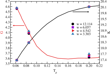
Shown in Fig. 1 are the shear modulus (left axis) and the bulk modulus (right axis) obtained from deforming the system (lines) and from the averages of the distributions of the local moduli (symbols) for different box sizes. Up to the mode coupling temperature $T_{\text{MCT}}$ the global shear modulus $G$ changes very little with decreasing parent temperature $T_{\text{p}}$. Below $T_{\text{MCT}}$ it increases with decreasing $T_{\text{p}}$, reaching a value approximately $27\%$ larger at the lowest parent temperature used. In contrast, the global bulk modulus $K$ monotonically decreases with decreasing $T_{\text{p}}$, reaching a value $7\%$ smaller at the lowest parent temperature than at $T_{\text{MCT}}$. The averages of the local shear $G^{\text{m}}$ and bulk $K^{\text{m}}$ moduli for different box sizes are very close to the moduli obtained from deformation. We do find, however, that at the largest parent temperature the averages of the shear moduli are slightly larger than the value obtained from deformation, with the difference increasing systematically with decreasing box size.

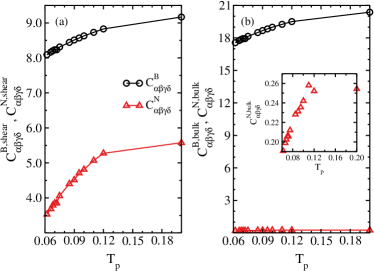
We note that, as shown in Fig. 2, for both of the global shear and the global bulk moduli the Born and fluctuation terms in $C_{\alpha\beta\gamma\delta}$ decrease with decreasing $T_{\text{p}}$. For the shear modulus, the fluctuation term decreases faster with decreasing $T_{p}$ than the Born term, and this leads to the increase in the shear modulus since the two terms are the same order of magnitude. However, for the bulk modulus the fluctuation term is an order of magnitude smaller than the Born term, and thus a decrease in the Born term leads to a decrease of the bulk modulus.

Figure 2: The dependence of the Born and fluctuation terms on the parent temperature. Inset: rescaled data for the bulk fluctuation term. Both Born and fluctuation terms decrease with decreasing parent temperature, for both shear (a) and bulk (b) moduli.

Although the average shear and bulk moduli are approximately independent of the box width $w$, one would expect to find some box width dependence of the width of the moduli distributions. The dependence of the width of the distribution relative on the box size is an important parameter in the fluctuating elasticity theory. Mizuno et al. found that the distributions of the individual shear moduli are almost identical and presented distributions averaged over the individual components. We found that the same fact is true for our system and also present distributions of the shear moduli averaged over the individual components.

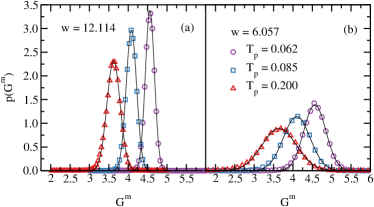
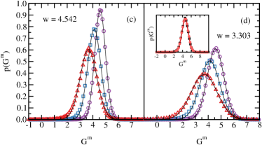
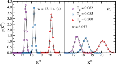
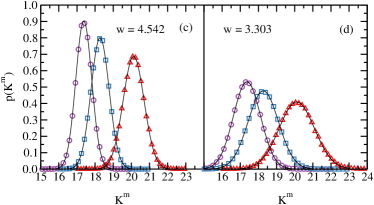
Shown in Fig. 3 are probability distributions of the local shear modulus $G^{\text{m}}$ calculated for (a) $w$ = 12.114, (b) $w$ = 6.057, (c) $w$ = 4.543, and (d) $w$ = 3.303 for three parent temperatures $T_{p}$ = 0.062 (circles), 0.085 (squares), and 0.2 (triangles). We note that there are no finite size effects, which we demonstrate in the inset to Fig. 3(d) by calculating the distribution for $N=48000$ and $N=192000$ for a box of the same size. However, as discussed in Ref. [Mizuno et al. (2013)], the $\left\langle\sigma_{\alpha\beta}^{m}\sigma_{\gamma\delta}\right\rangle$ term converges very slowly for large systems. To characterize the width we fit the distributions to a Gaussian distribution, $A\exp\{-0.5(G-G_{0})^{2}/\sigma^{2}\}$, where $G_{0}$ is the average shear modulus and $\sigma$ is the standard deviation. The fits are shown as straight lines in the figures. For all box sizes, including the smallest one with $w=3.303$ that only contains $\simeq 36$ particles, the shear moduli distributions are well described by Gaussian distributions.

We can see two trends. First, with increasing stability the distribution becomes narrower. This is easily seen since the peak of the distribution increases with decreasing width due to normalization of the distributions. Therefore, with increasing stability the glass becomes more uniform, in the sense that the local shear moduli vary less between different boxes. The other trend is that the width becomes broader with decreasing box size. This result is intuitively expected.

One noticeable property of some of these distributions is the appearance of regions with negative moduli. The regions with negative moduli are characterized as domains where the deforming force and the resulting response are in opposite directionsLakes et al. (2001), which suggests that these domains are unstable. However, with such small domains it is questionable if continuum elasticity is a valid description Tanguy et al. (2002). Overall, at each box size the distributions with higher averages and smaller standard deviations (i.e. the distributions of $T_{\text{p}}=0.062$) represent the more stable structureFan et al. (2014).

Figure 3: Distributions of local shear moduli for different box sizes: (a) $w=12.114$, (b) $w=6.057$, (c) $w=4.542$, (d) $w=3.303$. Each panel shows distributions for three different parent temperature, circles, $T_{p}=0.062$, squares, $T_{p}=0.085$ and triangles $T_{p}=0.200$. The solid lines show Gaussian fits to the distributions.

We also examined the distribution of the bulk modulus $K^{\text{m}}$, Fig. 4 for the same three parent temperature $T_{\text{p}}$ and box sizes $w$. We also find that the width of the distribution of $K^{\text{m}}$ decreases with decreasing parent temperature and increases with decreasing box size. The lines in the figures are fits to a Gaussian distribution. Again, these results points to the bulk modulus becoming more uniform with an increase of the stability. Since the bulk modulus is 3.5 to 5.5 times larger than the shear modulus (depending on stability), the change in the relative size of the distribution $\sigma_{\Gamma}/\Gamma$, where $\Gamma=G$ or $K$ is much less for the bulk modulus.

Figure 4: Distributions of local bulk moduli for different box sizes: (a) $w=12.114$, (b) $w=6.057$, (c) $w=4.542$, (d) $w=3.303$. Each panel shows distributions for three different parent temperature, circles, $T_{p}=0.062$, squares, $T_{p}=0.085$ and triangles $T_{p}=0.200$. The solid lines show Gaussian fits to the distributions.

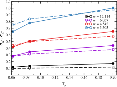
We summarize the parent temperature and box size dependence of the standard deviation of the distributions of the local moduli in Fig. 5. The closed symbols are the results for the shear moduli and the open symbols are results for the bulk modulus. The increase in $\sigma_{G^{m}}$ upon decreasing the box of size from $w$ = 12.114 to $w$ = 3.303 is a factor of 5.5 for $T_{p}$ = 0.2 and 5.8 for $T_{p}$ = 0.062. Similarly, the decreases of $\sigma_{G^{m}}$ with parent temperature for a fixed box size is 31% for $w$ = 12.114 and 35% for $w$ = 3.303.

We calculated the disorder parameter of fluctuating elasticity theory Schirmacher (2006); Schirmacher et al. (2007); Marruzzo et al. (2013), $\gamma_{G}=\rho w^{3}\sigma_{G^{m}}^{2}/\left<G^{m}\right>^{2}$ for the different box sizes. We found that the disorder parameter varies with box size. For our most stable glass, $T_{p}=0.062$, $\gamma_{G}=1.24$ for $w=12.1$ and $\gamma_{G}=0.90$ for $w=3.3$. The disorder parameters differ by approximately $38\%$. This box size dependence of the disorder parameter makes it unclear if this is a proper parameter to be used as input to a theory of excitations in glasses.

The disorder parameter does increase dramatically with decreasing stability for a fixed box size. The disorder parameter increases by a factor of 3.4-3.9, depending on box size, when we compare our most stable glass, $T_{p}=0.062$, to our least stable glass, $T_{p}=0.2$. For our least stable glass, disorder parameters are of similar magnitude as thouse found by Mizuno, Ruocco, and Mossa Mizuno et al. (2019) in their $T=0$ glass.

We note that the change in the variation of the local elastic moduli, i.e. of the heterogeneity of the local elasticity, with the changing stability found in this work is much larger than that estimated by Pogna et al. for hyperaged amber. In the latter study a decrease of only 5% was estimated upon a very large increase in the stability. We note that the change in the variation of the elastic constants reported by Pogna et al. was obtained indirectly, by fitting measured vibrational densities of states to the predictions of the fluctuating elasticity theory. Thus, the accuracy of their inferred change of the variation of the local elastic moduli depends on accuracy of the fluctuating elasticity model that they used. We find that there is probably a stonger dependence of the variation of the elastic constants on the glass’ stability than that inferred from fluctuating elasticity theory.

Figure 5: Dependence of the standard deviation of the local shear, $\sigma_{\text{G}^{\text{m}}}$, and bulk moduli, $\sigma_{\text{K}^{\text{m}}}$, on the parent temperature. The solid lines and filled symbols show $\sigma_{\text{G}^{\text{m}}}$ and the dashed lines and open symbols show $\sigma_{\text{K}^{\text{m}}}$. The standard deviation $\sigma_{\text{G}^{\text{m}}}$ increases by 67% for our smallest box size $w=3.303$ and 50% for our largest box size $w=12.114$. The standard deviation $\sigma_{\text{K}^{\text{m}}}$ increases by 33% for our smallest box size and 7.1% for our largest box size. Since $K>G$, this signifies a much larger relative change in $\sigma_{\text{G}^{\text{m}}}$ than $\sigma_{\text{K}^{\text{m}}}$.

To characterize the spatial correlations of local shear moduli, which also enter into the fluctuating elasticity theory Schirmacher et al. (2010), we calculated the correlation function

$$g_{GG}(r)=\sum_{m}\sum_{n}\left(\left<G^{m}G^{n}\right>-\left<G^{m}\right>\left<G^{n}\right>\right)\delta(r-|\mathbf{r}_{m}-\mathbf{r}_{n}|),$$ (8)

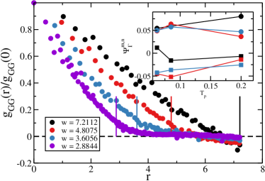
where $\mathbf{r}_{n}$ is the coordinate for the center of a box used to calculate the elastic moduli. We used 3000 particle systems to calculate $g_{GG}(r)$ and checked that the calculation was consistent with results for 48000 particle systems. It is important to recognize the fact that the boxes used in this calculation may overlap (in order to get results for distances $r$ smaller than the box size), and thus boxes may share some of the same particles and their elastic moduli are necessarily correlated. Therefore, there are trivial correlations in $g_{GG}(r)$ due to overlapping boxes. We show $g_{GG}(r)$ for our most stable glass, $T_{p}=0.062$, for four different box sizes $w$. We find that only the trivial correlations exists and $g_{GG}(r)$ decays to near zero at the size of the box, which is indicated by the vertical lines in the figure.

To explore further if there are spatial correlations for the shear modulus and the bulk modulus at every temperature and every box size, we calculate the cross correlations of neighboring non-overlapping boxes. To this end we calculate the correlation parameter

$$\Psi_{\Gamma}^{m,n}=\left|\left\langle\left(\frac{\Gamma^{m}-\Gamma}{\sigma_{\Gamma^{m}}}\right)\left(\frac{\Gamma^{n}-\Gamma}{\sigma_{\Gamma^{n}}}\right)\right\rangle_{m}\right|$$ (9)

where, $\left\langle\cdots\right\rangle_{m}$ denotes an average over all the boxes and box $n$ is one of the six nearest neighbors of box $m$ and $\Gamma=G$ or $K$. A correlation parameter close to $0$ indicates no significant correlation and a value of $1$ indicates perfect correlation. In the inset to Fig. 6 we show $\Psi_{G}$ (circles) and $\Psi_{K}$ (squares) for box sizes of $w=6.075$ (black), 4.542 (red), and 3.028 (blue). The values of $\Psi_{\Gamma}$ are all close to zero and there are no noticeable trends with box size or parent temperature. This leads us to conclude that the elastic moduli, calculated using this fully local approach, do not exhibit any spatial correlations. We also examined correlations of $G_{n}^{m}$ where $n=1...5$ found in Equation 7 and found the same trends, i.e. only trivial correlations. We note that there are other methods to calculate local elastic moduli Mizuno et al. (2013), and these other methods may indicate that the moduli are spatially correlated.

Figure 6: The spatial correlations of the shear modulus $G$ for a 3000 particle system and for our most stable glass, $T_{p}=0.062$. The different colors denote different box sizes $w=7.2112$ (black), 4.8075 (red), 3.6056 (blue), and 2.8844 (purple). The vertical lines indicate the box sizes. At these points the trivial correlations disappear. The inset shows the correlation parameter $\Psi_{G}^{m,n}$ (circles) and $\Psi_{K}^{m,n}$ (squares) for the box sizes $w=6.075$ (black), 4.542 (red), and 3.028 (blue) as a function of parent temperature ($N=48000$). The correlation parameter is small and there is no clear box size or parent temperature dependence.

This conclusion is at odds with the result of Gelin et al. Gelin et al. (2016) who reported that the elastic correlations decayed as $r^{-2}$ for a two dimensional glass-forming system different from the system used here. We note that Gelin et al. used a different way to define local elastic moduli. However, Mizuno and Ikeda Mizuno and Ikeda (2018) utilized the same method as Gelin et al. for yet another, different two dimensional system and found that the stress correlations decay as $r^{-2}$, but the elastic moduli correlations does not show the same long range correlations.

IV Conclusions

We examined the structural heterogeneities, including local and global elastic moduli, of glassy systems prepared from parent systems at different initial temperatures. Our calculations showed that the glass has a rather mild 27% increase of the local shear modulus, and a smaller 7% decrease on local bulk modulus compared to their values at the mode-coupling temperature with decreasing parent temperature. More importantly, we found that the local shear and the local bulk moduli become more uniform with decreasing parent temperature and thus stability of the glass. This finding is consistent with the recent report on the stability and sound attenuation of stable glassesWang et al. (2019). Sound attenuation increases with an increase in the fluctuations of the local elasticity, and hence with a decrease of the stability. Our results are in qualitative agreement with fluctuating elasticity theory Schirmacher (2006); Schirmacher et al. (2007); Marruzzo et al. (2013), which predicts an increase of sound attenuation and the observed Rayleigh-like $k^{4}$ scaling for small wavevectors Wang et al. (2019); Mizuno and Ikeda (2018).

Our results are also qualitatively consistent with recent experimental work by Pogna et al. on hyperaged amberPogna et al. (2019), which showed that the elastic matrix becomes more homogeneous with increased stability, corresponding to a smaller $T_{\text{p}}$ and a narrower moduli distribution in our study. However, we find that the local moduli are not spatially correlated. Pogna et al. inferred a 22% increase in the length scale characterizing elastic correlations. The same work reported on an increase of the elastic moduli fluctuation length scale in the more stable amorphous medium. This result, however, remains at variance with the findings of our study, where there is no discernible length scale associated with elasticity and there is no long range decay of elastic correlations. The lack of long range decay is also at odds with the study of Gelin et al.Gelin et al. (2016), but agrees with the conclusions of Mizuno and Ikeda Mizuno and Ikeda (2018).

Our results suggest that the current version of fluctuating elasticity theory is not a quantitatively accurate description of sound attenuation and the boson peak in amorphous solids, even though it makes qualitatively accurate predictions. A similar conclusion was drawn by Caroli and Lamaître Caroli and Lemaître (2019), who developed a full tensorial fluctuating elasticity theory and found that it underestimates the sound attenuation by about two orders of magnitude. Further theoretical work is warranted to properly describe the interplay of sound attenuation and elastic heterogeneities.

References

- Zeller and Pohl (1971) R. C. Zeller and R. O. Pohl, Phys. Rev. B, 1971, 4, 2029–2041.
- Stephens (1973) R. B. Stephens, Phys. Rev. B, 1973, 8, 2896–2905.
- Zaitlin and Anderson (1975) M. P. Zaitlin and A. C. Anderson, Phys. Rev. B, 1975, 12, 4475–4486.
- Pohl et al. (2002) R. O. Pohl, X. Liu and E. Thompson, Rev. Mod. Phys., 2002, 74, 991–1013.
- Mizuno et al. (2017) H. Mizuno, H. Shiba and A. Ikeda, PNAS, 2017, 114, 9767–9774.
- Wang et al. (2019) L. Wang, A. Ninarello, P. Guan, L. Berthier, G. Szamel and E. Flenner, Nat. Commun., 2019, 10, 26.
- Mizuno et al. (2013) H. Mizuno, S. Mossa and J.-L. Barrat, Phys. Rev. E, 2013, 87, 042306.
- Mizuno et al. (2016) H. Mizuno, S. Mossa and J.-L. Barrat, Phys. Rev. B, 2016, 94, 144303.
- Yoshimoto et al. (2004) K. Yoshimoto, T. S. Jain, K. V. Workum, P. F. Nealey and J. J. de Pablo, Phys. Rev. Lett., 2004, 93, 175501.
- Tsamados et al. (2009) M. Tsamados, A. Tanguy, C. Goldenberg and J.-L. Barrat, Phys. Rev. E, 2009, 80, 026112.
- Léonforte et al. (2006) F. Léonforte, A. Tanguy, J. P. Wittmer and J.-L. Barrat, Phys. Rev. Lett., 2006, 97, 055501.
- Mizuno et al. (2014) H. Mizuno, S. Mossa and J.-L. Barrat, PNAS, 2014, 111, 11949–11954.
- Gelin et al. (2016) S. Gelin, H. Tanaka and A. Lemaître, Nat. Mater., 2016, 15, 1177–1181.
- Caroli and Lemaître (2019) C. Caroli and A. Lemaître, Phys. Rev. Lett., 2019, 123, 055501.
- Fan et al. (2014) Y. Fan, T. Iwashita and T. Egami, Phys. Rev. E, 2014, 89, 062313.
- Mizuno et al. (2013) H. Mizuno, S. Mossa and J.-L. Barrat, Europhys. Lett., 2013, 104, 56001.
- Wagner et al. (2011) H. Wagner, D. Bedorf, S. Küchemann, M. Schwabe, B. Zhang, W. Arnold and K. Samwer, Nat. Mater., 2011, 10, 439–442.
- Mizuno et al. (2016) H. Mizuno, L. E. Silbert and M. Sperl, Phys. Rev. Lett., 2016, 116, 068302.
- Pogna et al. (2019) E. A. A. Pogna, A. I. Chumakov, C. Ferrante, M. A. Ramos and T. Scopigno, J. Phys. Chem. Lett., 2019, 10, 427–432.
- Schirmacher et al. (2007) W. Schirmacher, G. Ruocco and T. Scopigno, Phys. Rev. Lett., 2007, 98, 025501.
- Schirmacher et al. (2010) W. Schirmacher, C. Tomaras, B. Schmid, G. Baldi, G. Viliani, G. Ruocco and T. Scopigno, Condensed Matter Physics, 2010, 13, 23606.
- Mizuno and Ikeda (2018) H. Mizuno and A. Ikeda, Phys. Rev. E, 2018, 98, 062612.
- Moriel et al. (2019) A. Moriel, G. Kapteijns, C. Rainone, J. Zylberg, E. Lerner and E. Bouchbinder, arXiv:1905.03378, 2019.
- Ninarello et al. (2017) A. Ninarello, L. Berthier and D. Coslovich, Phys. Rev. X, 2017, 7, 021039.
- Grigera and Parisi (2001) T. S. Grigera and G. Parisi, Phys. Rev. E, 2001, 63, 045102.
- Gutiérrez et al. (2015) R. Gutiérrez, S. Karmakar, Y. G. Pollack and I. Procaccia, Europhys. Lett., 2015, 111, 56009.
- (27) http://lammps.sandia.gov.
- Plimpton (1995) S. Plimpton, J. Comp. Phys., 1995, 119, 1–19.
- Tanguy et al. (2002) A. Tanguy, J. P. Wittmer, F. Leonforte and J.-L. Barrat, Phys. Rev. B, 2002, 66, 174205.
- Lakes et al. (2001) R. S. Lakes, T. Lee, A. Bersie and Y. C. Wang, Nature, 2001, 410, 565–567.
- Schirmacher (2006) W. Schirmacher, Europhys. Lett., 2006, 73, 892–898.
- Marruzzo et al. (2013) A. Marruzzo, W. Schirmacher, A. Fratalocchi and G. Ruocco, Sci. Rep., 2013, 3, 1407.
- Mizuno et al. (2019) H. Mizuno, G. Ruocco and S. Mossa, arXiv:1905.10235v1, 2019.
- Wang et al. (2019) L. Wang, L. Berthier, E. Flenner, P. Guan and G. Szamel, Soft Matter, 2019, 7018–7025.