labelinglabel

An agglomerative hierarchical clustering method by optimizing the average silhouette width

Fatima Batool
ucakfba@ucl.ac.uk
Department of Statistical Science,
University College London, WC1E 6BT, United Kingdom

Abstract

An agglomerative hierarchical clustering (AHC) framework and algorithm named HOSil based on a new linkage metric optimized by the average silhouette width (ASW) index ( Rousseeuw [1987]) is proposed. A conscientious investigation of various clustering methods and estimation indices is conducted across a diverse verities of data structures for three aims: a) clustering quality, b) clustering recovery, and c) estimation of number of clusters. HOSil has shown better clustering quality for a range of artificial and real world data structures as compared to $k$-means, PAM, single, complete, average, Ward, McQuitty, spectral, model-based, and several estimation methods. It can identify clusters of various shapes including spherical, elongated, relatively small sized clusters, clusters coming from different distributions including uniform, t, gamma and others. HOSil has shown good recovery for correct determination of the number of clusters. For some data structures only HOSil was able to identify the correct number of clusters.
Key words and phrases: linkage measure, clustering quality, within and between cluster distances, estimation of number of clusters, combinatorial optimization, software

1 Introduction

Clustering is a widely used multivariate data analysis tool that aims at uncovering hidden underlying grouping structure in the data. It has become an essential data analysis procedure in various disciplines for different purposes, for instance, to organize the big, messy datasets for further analysis, to find important features, to explore the relationship between features, or to reduce dimensions. Some application areas include but are not limited to medical science, neuroscience, climatology, data mining, and computer vision.

In this article we have solved two major problems in cluster analysis simultaneously. The two problems are the estimation of number of clusters and finding the clustering solution. A clustering method can be defined by optimizing the objective function based on the ASW clustering quality index proposed by Rousseeuw [1987]. The motivation is that if the number of clusters estimated by an index are acceptable then the final clustering solution based on the criterion used by the index should also be acceptable. The advantage of this is that it will make the task of clustering somewhat simpler and straightforward and the users don’t have to deal with the two tasks separately. In particular, in this article the AHC framework has been considered based on the optimizing of the ASW. The new algorithm proposed based on this method is named as HOSil (Hierarchical Optimum Silhouette width).

Clustering methods can be broadly classified as the hierarchical methods and the non-hierarchical methods. The hierarchical methods return a sequence of clustering solutions whereas non-hierarchical, also known as partitional or flat clustering, returns a single clustering solution. The aforementioned clustering methods have several advantages over the latter, for instance, for some applications a sequence of clustering solutions might be more informative as compared to just a single solution.

Secondly, unlike most non-hierarchical algorithms there is no need to specify the number of clusters a priori, however, if the desired number of clusters is already known the partitioning can be stopped when the required clusters are obtained. The results of the hierarchical clustering are organized in a dendogram such that the clustering solution at each hierarchy is visible in a single diagram.

The standard hierarchical clustering methods are deterministic and can be further classified as agglomerative (bottom-up) and divisive (top-down) methods. In this work, an AHC framework has been developed by taking the bottom-up approach. In the beginning of the bottom-up AHC each observation is considered as a “singleton” cluster. Based on some measure of proximity between clusters the process of developing hierarchy by merging the clusters begins. The measure of proximity commonly known as linkage method can be measured in form of similarities or dissimilarities. We have proposed ASW (Rousseeuw [1987]) as a linkage measure and used it to merge the clusters. A distance measure for the inter-cluster pairs of observations used for the calculation of the linkage method, which are the functions of these pairwise distances, are needed to amalgamate clusters. We have used Euclidean distance between pairs of observations. After each merge the total number of clusters decreases by one.

After the construction of the dendogram the next task is to decide where to cut the dendogram or in other words decide upon the number of clusters. The advantage of using ASW as a linkage criterion is that it automatically gives the best number of clusters. The tasks of evaluation of clustering quality and estimation of number of clusters are closely related. Since the ASW is a clustering quality measure the idea here is to choose the number of clusters that give the best clustering quality. The dendogram is cut at the level where the maximum ASW value is obtained.

Organization

In §2 brief literature has been presented to ASW. In §3 the notations for this paper have been set up and the ASW index has been formalized. In §4 the optimum ASW based AHC method and algorithm have been proposed. Exploration of the proposed method has then been focused on—the kind of structures it can can handle and its comparisons with other methods. In §5 experiments have been set up. The performance of the HOSil algorithm has been evaluated in two respects a) for the estimation of number of clusters, b) for the clustering solution itself. The references to all the clustering methods, indices for the estimation of number of clusters, and their software implementation used in this work have been presented in §5. The simulation results have been presented in §8. In §7 the numerical complexity analysis of the HOSil has been considered. Real-life applications have been presented in §6. Finally, the study has been closed with conclusions and future directions for this work in §9. This article has an appendix and a supplementary file.

2 Related work

Rousseeuw [1987] has proposed ASW with the partitioning around medoid algorithm (PAM) to estimate number of clusters. The ASW is a well-reputed and trusted clustering quality measure. The index has been well received by the research community and is widely used for the estimation of the number of clusters. The ASW has been extensively used to estimate the optimal number of clusters (with a combination of various clustering methods), to compare the performance of clustering methods and for the quality assessment of clustering obtained from many clustering methods. Some empirical studies have also been designed to evaluate performance of the ASW in comparison with other famous indecies. Some examples include Recupero [2007], Kennedy et al. [2003], Hruschka and Ebecken [2003] and Lovmar et al. [2005]. For clustering quality measures, and clustering method comparisons see Liu et al. [2003], Reynolds et al. [2006], Ignaccolo et al. [2008] and Arbelaitz et al. [2013]. Campello and Hruschka [2006] have extended ASW to a fuzzy clustering regime. Some interesting variations and modifications have also been proposed, for instance, density based ASW by Menardi [2011] and the slope statistics by Fujita et al. [2014].

Van der Laan et al. [2003] have proposed PAMSIL algorithm which is a PAM-like (Rousseeuw [1987]) algorithm to maximize the ASW using medoids to find flat clustering. The PAM algorithm has two phases, namely, the build phase, and the swap phase. Van der Laan et al. [2003] first ran the build phase of PAM algorithm to get a set of $k$-medoids and then considered all possible swaps to further improve the values of objective function obtained in the build phase with an exception that their objective function did not try to optimize the distance of points from the nearest medoid but the ASW of the clustering.

3 Notational setup

The silhouette width (SW) for an object in data represents how well the object fits in its present cluster. Let $\pazocal{X}=\{x_{1},\dots,x_{n}\}$ be the data of size $n$ and $d$ be a distance function over $\pazocal{X}$ and $\mathcal{C}_{k}=\{C_{1},\dots,C_{k}\}$ a clustering identified by some clustering function $f_{k}$ on $\pazocal{X}$. Let $i$ represents the index for observations $x_{i}\in\pazocal{X}$. Let the clustering labels set be denoted by $\{l(1),\dots,l(n)\}\in\mathds{N}_{k}$ determined by $l(i)=r$, $r\in\mathds{N}_{k}$, $i\in\mathds{N}_{n}$ and cluster sizes are determined by $n_{r}=\sum_{i=1}^{n}1(l(i)=r)$, $r\in\mathds{N}_{k}$. For each objects $i\in\mathds{N}_{n}$ calculate

$$a(i)=\frac{1}{n_{{l(i)}}-1}\sum_{\begin{subarray}{c}l(i)=l(h)\\ i\neq h\end{subarray}}d(x_{i},x_{h}),\quad\text{and}\quad b(i)=\min_{r\neq l(i)}\frac{1}{n_{r}}\sum_{l(h)=r}d(x_{i},x_{h}).$$ (1)

For a given clustering $\mathcal{C}_{k}$, the silhouette width for a data object having index $i$, $i\in\mathds{N}_{n}$, is

$$S_{i}(\mathcal{C}_{k},d)=\frac{b(i)-a(i)}{\textrm{max}\{a(i),b(i)\}},$$ (2)

such that $-1\leq S_{i}(\mathcal{C}_{k},d)\leq 1$.

The SW averaged over all the members of a cluster can be used as a measure of a cluster’s quality. The ASW averages SW over all members of a dataset $\pazocal{X}$. It is a global quality measure for clustering. Formally, for the clustering $\mathcal{C}_{k}$ it can be written as follows:

$$\bar{S}(\mathcal{C}_{k},d)=\frac{1}{n}\sum_{i=1}^{n}S_{i}(\mathcal{C}_{k},d).$$ (3)

The best $k$ can be selected by maximising $\bar{S}(\mathcal{C}_{k},d)$ over $k$.

The ASW can be thought of as a combinational index because it is based on two concepts which are separation and compactness that define a unified concept of isolation. It is a ratio of inter-cluster variation and intra-cluster variation. It measures how homogeneous the clusters are, and what the separation between them is. Thus the ASW tells us about the coherent structure of clustering.

For a good clustering the dissimilarity “within” clusters should be less than the dissimilarity “between” clusters. Therefore, if $a(i)$ is much smaller than the smallest between clusters dissimilarity $b(i)$ we get evidence (larger $s(i)$, close to 1 is better in this case), that object $x_{i}$ is in the appropriate cluster. On the other hand, $s(i)$ close to -1, points towards the wrong cluster assignment for object $x_{i}$. In this case $a(i)>b(i)$, meaning that object “$i$” is more close to its neighbouring cluster than to its present cluster. A neutral case occurs when $s(i)\approx 0$, i.e., object $x_{i}$ is approximately equidistant from both, its present cluster and neighbouring cluster.

4 AHC based on optimum ASW linkage

Let $\pazocal{X}=\{x_{1},\dots,x_{n}\}$ be the dataset to partitioned, where $x_{i}$ represents the $i^{th}$ observation, and each $x_{i}$ represents a $p$-dimensional variable. We will here only consider crisp clustering, thus every object will belong to one cluster only and there will be no overlapping between clusters in the hierarchy. There will be $n$ total hierarchy levels. Let $k_{1},\cdots,k_{n}$ be the number of clusters in a clustering at each hierarchy level. Let the full hierarchy of $\pazocal{X}$ is given by $\mathcal{P}=\{\mathcal{C}^{1}_{n},\dots,\mathcal{C}^{n}_{1}\}$. The superscript in $\mathcal{C}^{l}_{k_{l}}\in\mathcal{P}$, where $l=1,\cdots,n$ represents the hierarchy level, and $k_{l}=n,(n-1),\cdots,2,1$ represents the number of clusters at each hierarchy level. In AHC we start with $n$ clusters in the beginning. Thus if $l$ represents a particular hierarchy level, then at $l=1$ we have $k_{l}=n$ clusters, i.e., each observation forms a separate cluster. The number of clusters subsequently reduce as hierarchy level proceeds. For simplicity assume that only one pair of clusters merges at each hierarchy level.

Let $\mathcal{C}^{l}_{k_{l}}=\{C^{l}_{1},\cdots,C^{l}_{k_{l}}\}$, where $C^{l}_{r}\in\mathcal{C}^{l}_{k_{l}}$, $r=1,\cdots,k_{l}$ represents an $r$-th cluster in a clustering at hierarchy level $l$. The members of a cluster at hierarchy level $l=1$ can be further written as $C_{1}^{1}=\{x_{1}\}$, $C_{2}^{1}=\{x_{2}\}$, $\dots$, $C_{n}^{1}=\{x_{n}\}$, thus $\mathcal{C}_{1}=\{\{x_{1}\},\{x_{2}\},\dots,\{x_{n}\}\}$ and at the $(n^{th})$ final hierarchy level, $\mathcal{C}_{1}^{n}=\{x_{1},x_{2},\dots,x_{n}\}$, such that $\mathcal{C}_{1}^{n}=\pazocal{X}$. Let $\gamma^{l}(x_{1},r),\dots,\gamma^{l}(x_{n},r)$, where $r=1,\cdots,k_{l}$ represent the clustering label vector at hierarchy level $l$. At a hierarchy level $l$, $r$ indicates to which cluster observation $x_{i}$ has been assigned.

The AHC clustering algorithms takes an input the pairwise dissimilarities between observations. The pairwise dissimilarities can be calculated using a distance function. A function $d:\pazocal{X}\times\pazocal{X}\rightarrow\mathds{R}^{+}$, is called a distance on $\pazocal{X}$ if, it satisfies the three properties stated as: (a) $\forall$ $x_{i},x_{h}\in\pazocal{X}$, where $i,h\in\mathds{N}_{n}$, $d(x_{i},x_{h})\geq 0$, (b) $\forall$ $x_{i}\in\pazocal{X}$, $d(x_{i},x_{i})=0$ , distance of an object to itself is zero, and (c) for $x_{i},x_{h}\in\pazocal{X}$, $d(x_{i},x_{h})=d(x_{h},x_{i})$.

An AHC algorithm has been is defined based on a linkage criterion that optimizes ASW. According to this criterion, two candidate clusters are merged together if this combination gives the maximum ASW as compared to all other combinations. At each hierarchy level all possible cluster merges have been tried out and those clusters are finally merged that give maximum ASW. HOSil can also be used to find the best number of clusters ($k$) for the data. According to this criterion a best $k$ will be the one that gives maximum value of ASW among all hierarchy level.

The algorithm can’t start from $l=1$. This is because for the calculation of $a(i):i\in C$ there should be at least one cluster in the clustering, with at least two observations and for calculation of $b(i)$ there should be at least two clusters in a clustering solution. Therefore, for $(l=1$, $k_{1}=n)$ and $(l=n$, $k_{l}=1)$ calculation of ASW is not possible. So we can start calculating ASW from at least $k_{2}=n-1$ and must stop at $r_{n-1}=2$. For $l=1$ the two closest observations are joined to form a cluster.

[htpb!]

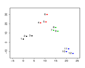
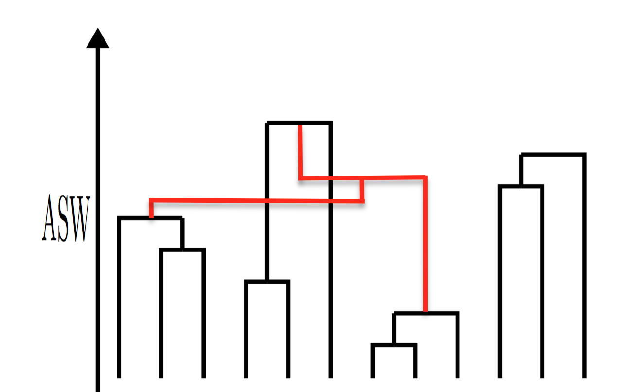
Figure 1-(a) shows a descriptive example of the algorithm using a dataset of 12 points. The left hand arrow represents the ASW values obtained from HOSil algorithm at each hierarchy level. Based on the maximum ASW principle, the best number of clusters for the data is 4 which looks intuitive. Using the ASW values obtained on each hierarchy a dendogram has been obtained for this clustering as shown in Figure 1-(b). The ASW values obtained at each hierarchy level are plotted on the vertical scale. These values are (k=11, l=1) 0.0613, (k=10, l=2) 0.2014, (k=9, l=3) 0.3177, (k=8, l=4) 0.3811, (k=7, l=5) 0.5049, (k=6, l=6) 0.5496, (k=5, l=7) 0.7117, (k=4, l=8) 0.7218, (k=3, l=10) 0.6408, (k=2, l=11) 0.6080. Note the two red horizontal dendrite connections which represent the decrease in the value of ASW at last two hierarchy level.

(a)

(b)

Figure 1: (a) An example with 12 instance in two dimensions to illustrate the HOSil algorithm.. (b) Dendogram representation of the HOSil clustering for the example datasets. The y-axis represents the ASW value obtained from HOSil clustering at each level of the hierarchy. The node from left to right represents the data points number 1 to 12 plotted in the left panel.

5 Experiments

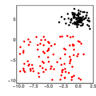
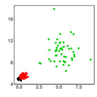
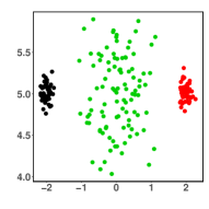
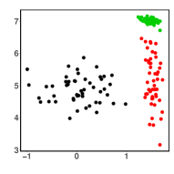
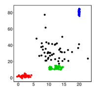
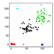
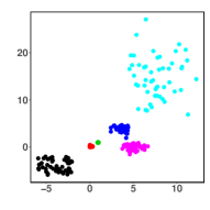
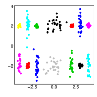
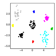
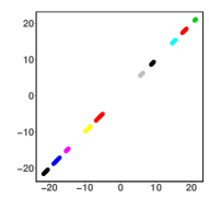
$\mathds{R}^{p}$ is used for the simulation of the data $\pazocal{X}$ in experiments, however the proposed algorithms works with the data from other spaces. The proposed algorithm also works with general distances, thus, specifying $\pazocal{X}$ belongs to some space $S$ characterised by distances $d:S\times S\mapsto\mathds{R}^{+}$, such that $\pazocal{X}$, the data is a subset of $S$ is enough for the formalism. Several data generating processes (DGP) having 2 to 14 distinct clusters, different clustering structures, characteristics and complexity have been defined to test the proposed method. These DGPs cover clustering scenarios having difficulties of various kinds, for instance, clusters from different distributions—assuming every individual cluster is coming from a single distribution with different variations among observations, equally and unequally sized clusters, clusters from skewed distributions, different types of clusters, for instance, spherical, non-spherical, elongated, close and far away clusters, i.e., the distance between the means of clusters are varied, nested clusters, clusters with correlated variables, different number of clusters and variables. In this article results from only 10 DGPs covering these features were presented. Figure 2h represents a plot of a dataset each, generated from these DGPs (see Table 1 for a complete list of distributions and parametric choices used to generate data).

Table 1: Parameters used in simulations. Simulations include clusters with Gaussian, skew Gaussian, t, non-central t, uniform, $\mathds{F}$, exponential, Beta, and Weibull distributions. Dimensions are generated independently and identically.

DGP	$k$	$p$	Distributions	Cluster size	n
Model 1	2	2	$\textrm{N}((0,5),I_{2})$, $\mathds{U}(-10,-1)^{\ast}$	100	200
Model 2	3	2	$\textrm{N}((0,5),0.1I_{2})$, $\textrm{N}((0.5,5.5),0.2I_{2})$, $\textrm{t}_{25}(5)$, $\textrm{t}_{25}(10)$	50,100,50	200
Model 3	3	2	$\textrm{N}((-2,5),0.1I_{2})$, $\textrm{N}((2,5),0.1I_{2})$, $\textrm{N}((0,5),0.5I_{2})$	50,50,100	200
Model 4	3	2	$\textrm{N}((1.5,7),0.1I_{2})$,$\textrm{N}((0,5),0.5I_{2})$, $\textrm{N}((1.5,5),(0.1,0,0,0.7))$	50	150
Model 5	4	2	$\mathds{U}(10,15)^{\ast}$, $\mathds{W}(10,4)^{\ast}$,$\textrm{t}_{7}(10)$, $\textrm{t}_{7}(30)$	50	400
			$\textrm{N}((2,2),I_{2})$, $\textrm{N}((20,80),(0.1,0,0,2))$
Model 6	5	2	$\mathds{F}_{(2,6)}(4)$, $\mathds{F}_{(5,5)}(4)$, $\chi^{2}_{7}(50)$, $\chi^{2}_{10}(80)$	50	250
			$\textrm{N}((100,0),0.9I_{2})$, $\textrm{t}_{40}(100)$, $\textrm{t}_{35}(150)$
			$\textrm{SN}(200,0.8,3,6)$,$\textrm{SN}(20,0.9,2,4)$
Model 7	6	2	$\mathds{U}(-6,-2)^{\ast}$, $\textrm{Exp}(10)^{\ast}$, $\mathds{W}(10,4)^{\ast}$, $\textrm{Gam}(15,2)^{\ast}$	50	300
			$\textrm{Beta}(2,3,120)^{\ast}$, $\textrm{SN}(5,0.6,4,5)$,$\textrm{SN}(0,0.6,4,5)$
Model 8	14	2	$\textrm{N}((0,2),0.5I_{2})$,$\textrm{N}((0,-2),0.5I_{2})$,$\textrm{N}((-4,-2),\Sigma)$	25	350
			$\textrm{N}((-3,-2),\Sigma)$, $\textrm{N}((-2,-2),\Sigma)$, $\textrm{N}((2,-2),\Sigma)$
			$\textrm{N}((3,-2),\Sigma)$, $\textrm{N}((4,-2),\Sigma)$; $\Sigma=(0.1,0,0,0.7)$
			$\textrm{N}((-4,2),\Sigma_{2})$, $\textrm{N}((-3,2),\Sigma_{2})$, $\textrm{N}((-2,2),\Sigma_{2})$
			$\textrm{N}((2,2),\Sigma_{2})$, $\textrm{N}((3,2),\Sigma_{2})$, $\textrm{N}((4,2),\Sigma_{2})$: $\Sigma_{2}=0.1I_{2}$)
Model 9	9	3	Unit circle centred at $(0,0,0)$ with 33 points	33, 25	233
			$\textrm{N}((-7,-0.2,-0.2),0.1I_{3})$, $\textrm{N}((0.2,-4,-4),0.1I_{3})$
			$\textrm{N}((0.5,3,3),0.1I_{3})$, $\textrm{N}((7,-1,-1),0.1I_{3})$
			$\textrm{N}((-5.5,2.5,2.5),\Sigma_{3})$
			$\textrm{N}((4.5,-3,-3),\Sigma_{3})$; $\Sigma_{3}=c(0.6,0.8,0.6)$
			$\textrm{N}((-4,-2.5,-2.5),\Sigma_{4})$;
			$\textrm{N}((5,1.5,1.5),\Sigma_{4})$; $\Sigma_{4}=c(0.4,0.3,0.4)$
Model 10	10	100	$\mu_{100}=(-21,-18,-15,-9,-6,6,9,15,18,21)^{\ast}$	20, 40, 60, 70,	490
			$0.05I_{100}$, $0.1I_{100}$, $0.15I_{100}$, $0.175I_{100}$, $0.2I_{100}$	50$\times$ 6

• For the covariance matrices $\Sigma_{3}$ and $\Sigma_{4}$ only main diagonal are mentioned. The off-diagonals entries are zero. The distributions with ^∗ shows the other cluster dimensions are distributed same. See Appendix Afor full definitions of the DGPs.

(a) Model 1

(b) Model 2

(c) Model 3

(d) Model 4

(e) Model 5

(f) Model 6

(g) Model 7

(h) Model 8

(i) Model 9

(j) Model 10

Figure 2: A dataset generated from each data generating process.

 

The simulation was done in R language (R Core Team [2019]). Along with the proposed algorithm, various widely applicable clustering algorithms have been applied with Euclidean distances, namely $k$-means—Forgy [1965], partitioning around medoids(PAM) —Kaufman and Rousseeuw [1987], hierarchical clustering algorithms with single linkage—Sneath [1957], complete linkage—Sorensen [1948], average linkage—Sokal and Michener [1958], Ward method—Ward Jr [1963], McQuitty methods—McQuitty [1966], spectral clustering —Ng et al. [2002], model-based clustering —Fraley and Raftery [1998]), and PAMSIL—Van der Laan et al. [2003] clustering algorithm. For all the hierarchical clustering methods function ‘hclust()’ available with R base package “stats” was used. For Ward’s method option “Wards.D2” for the method argument of ‘hclust()’ was used. For $k$-means and PAM functions ‘kmeans()’ (with nstart = 100) and ‘pam()’ also available through base “stats”, and “cluster” (version: 2.0.6, Maechler et al. [2017]), were used, respectively. For spectral and model-based clustering the packages ”kernlab” (version: 0.9.25, Zeileis et al. [2004]), and “mclust” (version: 5.2.3, Scrucca et al. [2017]) implementation, available through the ‘specc()’ and ‘Mclust()’ functions, respectively, were used. For PAMSIL the standalone C function written by Van der Laan et al. [2003] was used. For all the methods, the default settings were used except otherwise stated. $B=50$ datasets were generated for each DGP.

The estimation of number of clusters were also considered from several internal indices with combinations of several clustering methods. Seven clustering methods namely, $k$-means, PAM and AHC with five linkage methods have been applied with 11 different methods of estimation of number of clusters. In particular, Calinski and Harabasz (CH) Caliński and Harabasz [1974], Hartigan (H) Hartigan [1975], Krzanowski and Lai (KL) Krzanowski and Lai [1988], Gap Tibshirani et al. [2001], Jump Sugar and James [2003], Prediction strength (PS) Tibshirani and Walther [2005], Bootstrap instability (BI) Fang and Wang [2012], ASW, PAMSIL and HOSil methods to estimate number of clusters were used. In addition Bayesian Information Criterion (BIC) Schwarz et al. [1978] with model-based clustering method as implemented in “mclust” to estimate number of clusters was used.

The maximum number of clusters allowed for the estimations were 15. For H, CH, KL, and Gap package “clustersim” (version: 0.45.2, Walesiak and Dudek [2017]), for ASW “cluster” (Maechler et al. [2017]), for PS and BI “fpc” (version: 2.1.10, Hennig [2015]), and for the Jump method the R code provided by the author (see Sugar and James [2003] were used. Lastly, various transformation powers for the Jump method in simulation were used, particularly, $\hat{\delta}_{k}$ using $Y=p/2$, $Y=p/3$, $Y=p/4$, $Y=p/5$, $Y=p/6$ and $Y=p/7$, where $p$ denote the dimensions of the data.

6 Result and discussion

6.1 Clustering performance comparison

The ASW and corresponding ARI values are reported in Table LABEL:aswoaswsumma for the true known clusters. The discussion in this section is based on the average results obtained from simulation. The visual clustering results are presented in the supplementary file. In the following discussion whenever the term “size of cluster” is used, I mean to refer the number of observations in clusters. Some general conclusions are evident from the examination of Table LABEL:aswoaswsumma, as given below:

1. All the methods have produced much higher values of ASW as compared to the true ASW values.

2. No single method is best for the optimization of the ASW clustering and for obtaining the best ARI values.

3. It is not necessary that the best ARI values will be achieved for the best ASW clusterings, in fact for the majority of DGPs this is not the case.

Since PAMSIL is the direct competitor of HOSIL for the aim of optimization of the ASW index for clustering, therefore, some specific conclusions related to these two clustering methods drawn from the study are given below:

1. Although PAMSIL has produced the best ASW value among the method considered for nearly half of the DGP: 1, 2, 3, 5, 6, and 7. As far as the best ARI is considered PAMSIL only gave the best ARI for two DGPs: 6 and 7.

2. HOSIL has produced the best ASW values for 3 DGPs: 4, 8, and 9.

3. Although PAMSIL has shown better performance in terms of ASW values as compared to HOSIL for about 5 models, it has always produced lesser ARI values in comparison to HOSil, except for models 6 and 7.

4. The best ARI values obtained were from spectral clustering for model 1, model-based clustering for models 3, 4, and 5, PAMSIL for models 6 and 7, HOSIL for models 2 and 8. However, many methods gave the best ARI values for models 9 and 10.

However, many other interesting conclusions can be drawn about the performance of the clustering methods for each DGP. The discussion of the results present in the tables for each DGP individually is included in the supplementary file.

6.2 Estimation of number of clusters comparison

The results for the estimation of number of clusters ($\hat{k}$) are now presented. The results were analysed using graphical and tabular methods. First, for each DGP, a complete frequency count table was produced for 1 to 15 clusters, by noticing the number of clusters estimated against each run in the simulation. This produced 10 tables. These tables are provided in the supplementary file to this paper. From these tables a table was produced for only the true number of clusters for each DGP. This gives total frequency counts broken down by the DGPs of the correct number of clusters estimated by all the methods included in the study as reported in Table LABEL:aggregationofresults.

Table 2: Frequency table of indication of cluster estimated at correct level for all the indices in combination with all the methods for all DGPs.

DGPs	M1	M2	M3	M4	M5	M6	M7	M8	M9	M10
No.of dims.	2	2	2	2	2	2	2	2	3	100
No. of clusters	2	3	3	3	4	5	6	14	8	10	Overall
	H
Single	13	8	13	0	9	3	2	0	10	14	72
Complete	0	0	0	0	3	0	6	0	0	0	9
Average	1	3	10	12	8	11	0	0	18	0	63
Ward	0	0	0	1	8	1	2	0	10	0	22
McQuitty	0	0	0	1	9	1	2	0	10	0	23
kmeans	3	24	1	0	16	16	6	0	2	0	68
PAM	3	24	1	0	16	17	6	0	2	0	69
											326
	CH
Single	39	8	20	0	0	9	1	24	50	20	171
Complete	37	11	1	0	1	0	0	0	36	0	86
Average	33	2	15	3	0	6	0	23	46	2	130
Ward	34	4	2	0	0	3	0	6	40	0	89
McQuitty	34	4	2	0	0	3	0	6	40	0	89
kmeans	36	3	0	2	1	11	5	6	2	2	68
PAM	29	0	0	0	0	0	0	2	24	0	55
											688
	KL
Single	3	4	6	6	5	9	4	0	0	0	37
Complete	2	3	4	13	7	11	0	0	2	0	42
Average	2	5	0	1	9	3	6	0	0	0	26
Ward	1	3	8	8	14	1	4	0	0	0	39
McQuitty	1	3	8	8	14	1	4	0	0	0	39
kmeans	22	5	3	3	10	6	6	0	16	2	73
PAM	7	6	12	0	8	4	12	0	2	0	51
											307
	Gap
Single	36	8	20	0	2	9	0	0	50	0	125
Complete	18	15	17	30	10	26	0	0	36	0	152
Average	19	7	44	32	10	45	0	0	24	0	181
Ward	28	14	19	28	9	29	0	0	30	0	157
McQuitty	26	14	18	28	8	30	0	0	38	0	162
kmeans	11	12	9	18	16	29	0	0	0	0	95
PAM	12	1	6	13	1	24	2	0	6	0	65
											937
	Jump
$p$/2	1	0	14	0	0	28	19	12	50	26	150
$p$/3	50	0	50	25	10	49	40	12	50	1	287
$p$/4	7	0	50	1	22	50	37	12	50	0	229
$p$/5	0	0	10	0	26	50	0	5	50	0	141
$p$/6	0	0	0	0	0	49	0	0	50	0	99
$p$/7	0	0	0	0	1	7	0	0	50	0	58
											964
	PS
Single	3	32	2	5	2	6	0	0	46	46	142
Complete	2	0	0	0	1	43	0	0	18	50	114
Average	28	7	0	20	2	43	0	0	48	46	194
Ward	44	1	0	29	0	50	0	0	50	50	224
McQuitty	3	1	0	0	1	40	0	0	48	48	141
kmeans	50	1	50	42	0	3	0	0	0	0	146
PAM	44	31	1	45	2	50	45	0	50	50	318
											1279
	BI
Single	0	4	0	6	0	3	3	1	44	0	61
Complete	0	0	0	0	0	24	0	1	6	0	31
Average	2	0	0	3	0	43	0	0	48	0	96
Ward	28	1	0	26	1	45	0	0	50	0	151
McQuitty	0	0	0	0	0	31	0	3	30	0	64
kmeans	50	0	50	23	0	9	0	1	0	0	133
PAM	32	0	0	44	7	50	8	1	50	0	192
											728
	ASW
Single	39	8	20	0	1	10	1	23	50	50	202
Complete	50	12	19	22	1	36	0	2	50	50	242
Average	50	5	50	36	1	48	0	22	50	50	312
Ward	48	5	22	23	2	44	0	11	50	50	255
McQuitty	48	5	22	23	2	44	0	11	50	50	255
kmeans	50	0	50	48	5	38	17	7	4	50	269
PAM	50	0	50	49	8	50	40	9	50	50	356
											1891
	BIC
Model-based	43	1	50	50	33	17	4	0	50	50	298
PAMSIL	50	0	50	44	9	50	47	1	50	50	351
HOSil	50	1	50	44	5	50	48	21	50	50	369

Based on the true number of clusters’ determination, the performance of the H and KL indices was not good for the majority of the models included in the study. The CH method performed well only for very few models and that was only for one or two clustering methods. The Jump method also estimated correct number of clusters for a very few models (never for Models 2, 8) and very low counts for (Models 5 and 10). The results for the Gap method were below average (less than half times) for the majority of the models included in the analysis. The BI and PS also performed poorly for majority of the models except for a few of them with one or two clustering methods only. Model-based clustering has estimated $\hat{k}$ other than expected for Models 2, 5, 6, 7, and 8. HOSil clustering estimated $k$ other than the true $k$ for Models 2 and 5. PAMSIL was also not able to estimate the correct number of clusters for the two models mentioned for HOSil and in addition Model 8.

Top performing indices

Based on the performance aggregated for all DGPs an overall ranking can be created. Given the fact that the total frequency count is 369, HOSil has provided the best performance for the recovery of the true number of clusters. ASW index with PAM clustering method is the second best performing combination with 356 counts. PAMSIL is third in this list with 351 counts. Further, ASW index with average linkage being forth, Model-based clustering with BIC being the fifth, and ASW index with $k$-means clustering is on the sixth rank.

7 Runtime

HOSil is implemented in C++ and has an interface for its call in the R language using the Rcpp package (Eddelbuettel et al. [2011]). The runtime of HOSil is compared with the existing algorithms for all the simulated datasets. The computations were done on the UCL high performance and throughput computing facilities using Legion cluster. Table 3 contains the runtime of HOSil. The time reported here does not include the time for distance calculations. The proposed algorithm’s performance for retrieving an accurate clustering is good with the advantage that it can also estimate the number of clusters provided the time it takes. In addition, note that the larger $p$ is not a problem for the algorithm (for instance see DGP 10) because it’s not represented in distances. Also, note that the time reported in the Table 3 is to build the full hierarchy, i.e., from 2 to $(n-1)$ clusters. However, the algorithm is implemented in such a way that if $k$ is known, then the algorithm can be stopped at the desired hierarchy level which will significantly reduce the time.

Table 3: Time taken by HOSil clustering algorithm for DGPs.

DGP	$k$	$p$	$n$	runtime
Model 1	2	2	200	11m
Model 2	3	2	200	10.6m
Model 3	3	2	200	10m
Model 4	3	2	250	35m
Model 5	4	2	200	10m
Model 6	5	2	250	32.5m
Model 7	6	2	300	2.7h
Model 8	14	2	350	6h
Model 9	9	3	233	43m
Model 10	10	100	250	1h

• m = minutes, h = hours. Note that R returns a runtime in seconds. The reported run time here is subject to approximation to minutes and hours. The runtime is the averaged over all runs.

8 Applications

8.1 Tetragonula bee data clustering

In this section, the species delimitation of Franck et al. [2004] dataset was considered using HOSil. The dataset gives the genetic information of 236 species among bees at 13 microsatellite loci from eastern Australia and between Indian and Pacific oceans. The 13 variables are categorical. The purpose of clustering for this data is to find how many bee species are present.

The distance measure used was the ”shared allele dissimilarity” particularly designed for calculation of genetic dissimilarities between species by Bowcock et al. [1994], and is implemented through the package ‘prabclus’ (Hennig and Hausdorf [2015]).

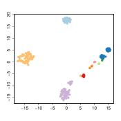
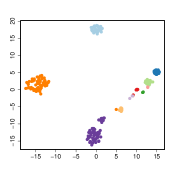
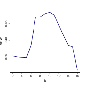
Since a desirable characteristic to species delimitation could be cluster separation, and the ASW linkage is based on the concept of cluster separation and compactness, therefore, it makes sense to apply HOSil to the bees dataset for clustering. According to HOSil the best number of species present in the data is 10. The 4 best ASW values obtained together with adjusted rand index in bold with the number of clusters were 0.48406(0.914795, k = 10), 0.47999(0.91082, k = 9), 0.47673(0.834181, k = 11), 0.47058(0.907194, k = 8). As evident from the Figure 3c as well, the value of the ASW monotonically decreases for the k before and after k=10(see Figure 3c for k = 2 to 16).

The dataset is ploted against the delimitation provided by Franck et al. [2004], and HOSil results in two dimensions with the t-distributed stochastic neighbor embedding (t-SNE) available through an R package ‘Rtsne’ (Krijthe et al. [201]) in Figure 3.

(a) short for lof

(b) short for lof

(c) short for lof

Figure 3: t-SNE visualization of the Tetragonula dataset in two dimensions (a) colours represent the species delimitation provided by Franck et al. [2004] (b) colours represent the HOSil clustering results. (c) ASW value obtained from HOSil for 2 to 16 clusters. The maximum value of ASW is obtained at k=10.

8.2 French rainfall data clustering

Finding spatial or temporal patterns in climate datasets based on statistical techniques is of crucial importance for climatologists. The data used in Bernard et al. [2013], available through the software they wrote, has been considerd for the clustering of french weather into climate regions based on rainfall precipitation maxima observed at the stations. Bernard et al. [2013] proposed a clustering algorithm based on a combination of PAM algorithm and a distance measure for geostatistics data called the F-madogram (Cooley et al. [2006]). The data is for 92 French weather stations for the three months of fall, from September to November for 19 years.The purpose of clustering is to find the pattern among stations i.e., spatial clustering based on the fact that if the local conditions at two weather stations are similar, then the two maxima precipitation series at these stations are not independent and the two weather stations should be in one cluster.

The application of the HOSil algorithm to this data offers certain benifts as compared to the algorithm proposed in Bernard et al. [2013]. All the statistical clustering methods based on averages can not be applied to such datasets due to the fact that the definition of the distances for the maxima of time series dependents on the generalised extreme value (GEV) family of distributions (see Bernard et al. [2013]). HOSil does not make use of any kind of cluster representatives like centroids for clustering. It works with the individual data points. Therefore, it will deal directly with the time series of maxima rather than any kind of averages of these maxima. In addition, it also offers another advantage that it can estimate number of clusters as well unlike the necessary preprocessing step in Bernard et al. [2013]’s method.

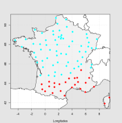
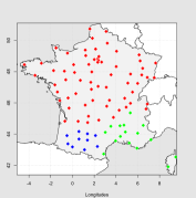
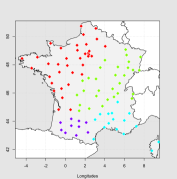
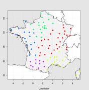
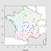
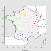
The resulting clusterings from HOSil algorithm are displayed in Figure 4 for 2 to 7 clusters. For numbers of clusters two HOSil has classified french weather stations in (clock-wise) the east, south and south-west regions of France together in a cluster (red cluster in Figure 4a, say cluster 1), and from the south-west, north, and all the way to the east in the other cluster (blue cluster). The two highest mountain peaks —the Alps in the east, and the Pyrenees in the south of France are clustered together (cluster 1). The two weather stations in Corsica, which has the third highest mountain peaks, are also classified in this cluster. Since PAM looks for equally sized clusters, Bernard et al. [2013] got an almost equal number of weather stations in the north and south clusters, dividing France along the Loire valley line. HOSil for three clusters further separates cluster 1 in south-east and south-west fashion i.e., isolating the regions with the Alps and Pyrenees. For four clusters, HOSil has further isolated central France from the northern region. For the five clusters the upper northern region is further divided into west to north-west, and from north-west to the north regions.

In terms of the number of clusters, the highest ASW value was obtained for k=2 (0.1390), indicating the strongest weather pattern, meaning that the climates of these two regions differ most significantly in the country. The second best ASW value was achieved for k=3(0.1251). After that, the strongest climate pattern was observed for k=7(0.1166). The fourth best ASW was obtained for k=6(0.1135).

(a) short for lof

(b) short for lof

(c) short for lof

(d) short for lof

(e) short for lof

(f) short for lof

Figure 4: Clustering results from HOSil algorithm. Panels from (a) - (f) denote clustering against k=2 to k=7.

8.3 Identification of cell population

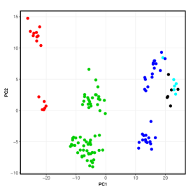
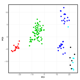
Identification of cell types in several tissues and organs from the mass of heterogeneous cells is an important task in cell biology. This is considered as the first step in the biological analysis of the most recently known technique, single-cell RNA sequencing (scRNA-seq). It is a way to analyse an individual cell and it can inform how each cell is different from the other. The data by Goolam et al. [2016] has been considered for clustering using HOSil. This data is the study of pre-implantation development of 124 cells of mouse embryos. There are 5 distinct cell types. 2-cell(16 samples), 4-cell(64 samples), 8-cell(32 samples), 16-cell(6 samples), and 32-cell(6 samples).

For the low-level analysis of data, i.e, quality control, normalization and dimensionality reduction, the R libraries “scater” McCarthy et al. [2017] and “scran” Lun et al. [2016] were used which are available through Bioconductor for scRNA-seq data. Euclidean distances between cells to perform clustering were used. The first three principled components of the dataset is plotted in Figure 5. The colour represents the true cell classification by the authors.

Table 4 shows the results for this data. It is evident from the table that all the methods have produced much higher values of the ASW as compared to the true values. The spectral clustering method gave very low value of ASW. $k$-means, PAM, and model-based clustering have also produced lower values of ASW as compared to other methods with very low ARI values. These methods were also not able to determine the correct number of clusters. The average linkage, Wards clustering, and HOSil methods have produced the highest ASW values with the best ARI values (see Table 4 for values). The average linkage, Wards clustering, and HOSil methods have also estimated correct numbers of clusters.

(a)

(b)

Figure 5: Data plots of first three principal components. Shown in red are 2-cell, green are 4-cell, blue are 8-cell, black are 16-cell and light blue are 32-cell stages.

Table 4: Goolam et al. [2016] data clustering results.

	True k		Estimated k
Methods	ASW	ARI	ASW	ARI	$\hat{k}$
True label	0.4905
k-means	0.5502	0.5439	0.5995	0.8831	3
PAM	0.5502	0.5439	0.6365	0.8602	4
average	0.6668	0.9097	0.6668	0.9097	5
Ward’s	0.6668	0.9097	0.6668	0.9097	5
model-based	0.5502	0.5439	0.6365	0.8602	4
spectral	0.2617	0.6365	0.3290	0.8602	4
BIC-mb	-	-	0.5925	0.4750	8
HOSil	0.6668	0.9097	0.6668	0.9097	5

9 Final remarks and future work

In this paper, a new AHC methodology was introduced, implemented through the HOSil algorithm. The approach was based on the development of the linkage criterion based on the ASW index. A monte carlo simulation of 11 procedures for determining the number of clusters paired with 7 clustering methods was conducted. For each of these combinations, 10 data structures were used.

HOSil can correctly identify a variety of clustering structures other than those presented here. Several other real and artificial structures were used to experiemnt. For instance, HOSil can return the desired clustering structures for the four shapes and smiley data from the R package “mlbench” (version: 2.1.1, Leisch and Dimitriadou [2010]), 2 diamonds, Hepta, and Tetra data from the fundamental clustering problems suite (FCPS) of Ultsch [2005]. It can also estimate the correct number of clusters for these datasets except for the smiley dataset. The smiley dataset contains two Gaussian eyes, one trapezoid nose and a parabolic mouth. For this data HOSil has divided the mouth into many small compact clusters. The reason for this is that the mouth cluster has bigger within cluster distances as compared to other clusters. In order to get a good ASW value, the within-cluster dissimilarities should be small as compared to between clusters dissimilarities. In case of the wide spread of observations within clusters i.e., large distances between clusters the small within-cluster dissimilarities requirement of ASW index dominates and it splits this bigger cluster into smaller clusters such that rather than having one cluster with bigger within-cluster distances it prefers to split this cluster into nicely compacted smaller clusters.

For this same reason HOSil can not identify clustering structures like Lsun data from FCPS. For the Aggregation (Gionis et al. [2007]) dataset it has identified all the clusters correctly except it has divided the moon-like cluster into two clusters, and has combined the two spherical clusters in one cluster for 7-cluster solution.

HOSil can also identify the correct data structures as well as recover the correct number of clusters for the datasets named “two elongated clusters in three dimensions”, “two close and elongated clusters in three dimensions”, and “three clusters in a microarray-like setting” in Tibshirani and Walther [2005].

Statement like HOSIL “can only produce equally sized spherical clusters” is not correct. HOSil can handle, to some extent, the variations among within cluster separations, and small sized clusters in the presence of bigger sized clusters. This also depends upon the difference between the means of clusters. However, unfortunately I am unable to offer more exact statements in this regards and quantify these factors.

HOSil can not handle overlapping data structures, and if a HOSil clustering is applied to such dataset it will produce well-separated clusters of equal or unequal sizes. A small study to learn the effect of various distance metrics on HOSil has been conducted. In the study, the Manhattan, Euclidean, and Minkowski distances have been included to observe the differences in the clustering results obtained by the proposed algorithm and other existing methods. Overall, from all the methods the optimization performance gained from Minkowski metric is the highest. The ASW values obtained for all the clustering methods showed same trend across DGPs. The values obtained from the Minkowski metric were greater than the Euclidean metric, and the values obtained from the Euclidean metric were greater than the Manhattan metric. A more systematic study—extended to other data spaces, distance metrics and more DGPs—is needed, in order to be able to make some in-depth analyses and generalized conclusions to some extent.

It is worthwhile to look for some fast approximations to implement ASW based linkage criterion or to improve the HOSil’s performance potential computationally for the datasets of bigger sizes. In this regard, I am working to reduce the computational time complexity of the HOSil algorithm. I am also working to extend the dendogram implementation to HOSIL to visualize the full hierarchy produced by the algorithm.

Appendix A Definition of data generating processes

For the data generating processes (DGPs) several probability distributions have been used. I first define the notations for these distributions. Let $N_{p}(\mu_{p},\Sigma_{p\times p})$ represents the $p$-variate Gaussian distribution with mean $\mu_{p}$ and covariance matrix $\Sigma_{p\times p}$. Let $SN(\zeta,\omega,\alpha,\tau)$ represent a skew Gaussian univariate distribution with $\zeta,\omega,\alpha,\tau$ as location, scale, shape and hidden mean parameters of the distribution respectively. Let $\mathds{U}(a,b)$ represent the uniform distribution defined over the continuous interval $a$ and $b$. Let $t_{v}$ represent Student’s $t$ distribution with $v$ degrees of freedom. Let $t_{r}(\nu)$ represent the non-central $t$ distribution with $r$ degrees of freedom and $\nu$ be the non-centrality parameter. Let $\textrm{Gam}(\alpha,\beta)$ represent Gamma distribution where $\alpha$ and $\beta$ are shape and rate parameters, respectively. Let $\textrm{NBeta}(v_{1},v_{2},\lambda)$ represents the non-central Beta distribution of Type-I with $v_{1},v_{2}$ be two shape parameters and $\lambda$ being the non-centrality parameter. Let $\textrm{Exp}(\lambda)$ represent the Exponential distribution with $\lambda$ being the rate parameter. Let $\mathds{F}_{(v_{1},v_{2})}(\lambda)$ represent the non-central $F$ distribution with $v_{1},v_{2}$ degrees of freedom and $\lambda$ be the non-centrality parameter. Let $\mathds{W}(\tau,\zeta)$ represent the Weibull distribution with $\tau,\zeta$ as shape and scale parameter, respectively. Let $I_{p}$ be the identity matrix of order $p$, where $p$ represents the number of dimensions. The DGPs are defined as below.

• Model 1 Two clusters of equal sizes are generated in two dimensions coming from different distributions. 100 observations are generated from the Gaussian distribution with identity covariance matrix centred at (0, 5). 100 observations drawn from $\mathds{U}(-10,1)$ independently along both dimensions. The result is one compact spherical cluster located at the corner of a uniformly distributed cluster.

• Model 2 Three clusters of unequal sizes and variations were generated in two dimensions. Two clusters were generated from independent bi-variate Gaussian distributions with 50 and 100 observations centred at (0, 5) and (0.5, 5.5), respectively, with covariance matrix as $0.1I_{2}$ and $0.2I_{2}$ respectively. The third cluster with 50 observations was generated from a non-central $t$ distribution with $t_{25}(5)$ and $t_{25}(10)$ independently. The clusters are of such nature that the generated non-central $t$ cluster has a wider spread than the two Gaussian clusters which were kept close to each other as compared to the bigger spread cluster.

• Model 3 Three Gaussian clusters in two dimensions of unequal variations. The clusters contains 50, 50, and 100 observations, with covariance matrices as $0.1I_{2}$, $0.1I_{2}$ and $0.5I_{2}$, while the clusters are centred at (-2, 5), (2, 5), (0, 5), respectively. The result is one bigger, spherical widely spread cluster located between two small, spherical and compact clusters.

• Model 4 Three Gaussian clusters in two dimensions of equal sizes, different variations and different shapes. 50 observations were generated from (0, 5) with covariance matrix as $0.5I_{2}$. 50 observations were generated from Gaussian distribution with means (1.5, 5) with covariance matrix as $\Sigma=\begin{bmatrix}0.1&0\\ 0&0.7\end{bmatrix}$. 50 observations were generated from (1.5, 7) with co-variance matrix as $0.1I_{2}$. The clusters look like a wider spread spherical cluster located left to the vertical cluster and a smaller compact cluster located just at the top of the vertical cluster.

• Model 5 Four clusters of equal sizes each having 50 observations were generated in two dimensions. One cluster was generated from independent non-central $t$ distributed variables with parameters $t_{7}(10)$ and $t_{7}(30)$. One cluster was generated from $\mathds{U}(10,15)$ independently along both dimensions. One cluster was generated from bivariate normal distribution parametrized by mean (2, 2), and covariance $I_{2}$ generated independently across both dimensions. The fourth cluster is also from independent bivariate Gaussian distributions parametrized by, mean (20, 80) with covariance matrix $\Sigma=\begin{bmatrix}0.1&0\\ 0&2\end{bmatrix}$.

• Model 6 Five clusters in two dimensions from different distributions. The clusters are parametrized from Chi-squared, $\mathds{F}$, $t$, Gaussian and skewed Gaussian distributions as $\chi^{2}_{7}(50)$ and $\chi^{2}_{10}(80)$, $\mathds{F}_{(2,6)}(4)$ and $\mathds{F}_{(5,5)}(4)$, $t_{40}(100)$ and $t_{35}(150)$, $N((100,0),0.9I_{2})$, $SN(20,0.9,2,4)$ and $SN(200,0.8,3,6)$. The clusters contains 50 observations each and were generated independently along both dimensions.

• Model 7 6 clusters from different distributions in two dimensions. The clusters are parametrized as $\mathds{U}(-6,-2)$, $\textrm{Exp}(10)$, $\textrm{Beta}(2,3,120)$, $\mathds{W}(10,4)$, $\textrm{Gam}(15,2)$ in both dimensions, whereas one cluster from $SN(5,0.6,4,5)$ along first dimension and $SN(0,0.6,4,5)$ across second dimension. The clusters contains 50 observations each and were generated independently along both dimensions.

• Model 8 Fourteen Gaussian clusters in two dimensions. Two clusters were generated with 25 observations each having common co-variance matrix as $0.5I_{2}$ centred at (0, 2) and (0, -2). Six clusters were generated with 25 observations each having common covariance matrices as $\begin{bmatrix}0.1&0\\ 0&0.7\end{bmatrix}$. The clusters are centred at (-4, -2), (-3, -2), (-2, -2), (2, -2), (3, -2), and (4, -2). The remaining six clusters have common covariance matrix as $0.1I_{2}$ and 25 observations each centred at (-4, 2), (-3, 2), (-2, 2), (2, 2), (3, 2), and (4, 2).

• Model 9 8 Gaussian clusters surrounding a cluster formed by uniformly distributed points in a unit circle. The unit circle contains 33 observations and is centred at [0, 0, 0]. The 8 Gaussian clusters contain 25 observations each. Four clusters are centred at (-7, -0.2, -0.2), (0.2, -4, -4), (0.5, 3, 3), and (7, -1, -1) with a common covariance matrix as $0.1I_{3}$. Two clusters are centred at (-5.5, 2.5, 2.5) and (4.5, -3, -3) with a common covariance matrix $\begin{bmatrix}0.6&0&0\\ 0&0.8&0\\ 0&0&0.6\end{bmatrix}$. Two clusters are centred at (-4, -2.5, -2.5) and (5, 1.5, 1.5) with a common covariance matrix $\begin{bmatrix}0.4&0&0\\ 0&0.3&0\\ 0&0&0.4\end{bmatrix}$.

• Model 10 10 clusters in 100 dimensions. The clusters are centred at -21, -18, -15, -9, -6, 6, 9, 15, 18, 21. The clusters are in 100 dimensions such that the 100 dimensional mean vectors of these values were generated for all clusters. The number of observations for these ten clusters are 20, 40, 60, 70, and 50 each for six of the remaining clusters. The number of observations for the means of clusters were not fix. Any cluster can take any number of observations from these such that any six clusters have equal number of observations i.e., 50 and the remaining four has different observations each, which is one out of 20, 40, 60, 70 values. The total size of the data is always 490 observations. The covariance matrix for each of these clusters is one out of 0.05$I_{100}$, 0.1$I_{100}$, 0.15$I_{100}$, 0.175$I_{100}$, 0.2$I_{100}$ matrices. The covariance matrix for each cluster was chosen randomly with replacement out of these, such that as a result, all the clusters can have same covariance matrix, two or more clusters can have same covariance matrix or all of the 10 clusters can have different same covariance matrices.

References

- Arbelaitz et al. [2013] Arbelaitz, O., I. Gurrutxaga, J. Muguerza, J. M. Pérez, and I. Perona (2013). An extensive comparative study of cluster validity indices. Pattern Recognition 46(1), 243–256.
- Bernard et al. [2013] Bernard, E., P. Naveau, M. Vrac, and O. Mestre (2013). Clustering of maxima: Spatial dependencies among heavy rainfall in france. Journal of Climate 26(20), 7929–7937.
- Bowcock et al. [1994] Bowcock, A. M., A. Ruiz-Linares, J. Tomfohrde, E. Minch, J. R. Kidd, and L. L. Cavalli-Sforza (1994). High resolution of human evolutionary trees with polymorphic microsatellites. Nature 368(6470), 455–457.
- Caliński and Harabasz [1974] Caliński, T. and J. Harabasz (1974). A dendrite method for cluster analysis. Communications in Statistics-Theory and Methods 3(1), 1–27.
- Campello and Hruschka [2006] Campello, R. J. and E. R. Hruschka (2006). A fuzzy extension of the silhouette width criterion for cluster analysis. Fuzzy Sets and Systems 157(21), 2858–2875.
- Cooley et al. [2006] Cooley, D., P. Naveau, and P. Poncet (2006). Variograms for spatial max-stable random fields. In Dependence in probability and statistics, pp. 373–390. Springer.
- Eddelbuettel et al. [2011] Eddelbuettel, D., R. François, J. Allaire, J. Chambers, D. Bates, and K. Ushey (2011). Rcpp: Seamless R and C++ integration. Journal of Statistical Software 40(8), 1–18.
- Fang and Wang [2012] Fang, Y. and J. Wang (2012). Selection of the number of clusters via the bootstrap method. Computational Statistics & Data Analysis 56(3), 468–477.
- Forgy [1965] Forgy, E. W. (1965). Cluster analysis of multivariate data: efficiency versus interpretability of classifications. Biometrics 21, 768–769.
- Fraley and Raftery [1998] Fraley, C. and A. E. Raftery (1998). How many clusters? which clustering method? answers via model-based cluster analysis. The Computer Journal 41(8), 578–588.
- Franck et al. [2004] Franck, P., E. Cameron, G. Good, J. Y. Rasplus, and B. Oldroyd (2004). Nest architecture and genetic differentiation in a species complex of australian stingless bees. Molecular Ecology 13(8), 2317–2331.
- Fujita et al. [2014] Fujita, A., D. Y. Takahashi, and A. G. Patriota (2014). A non-parametric method to estimate the number of clusters. Computational Statistics & Data Analysis 73, 27–39.
- Gionis et al. [2007] Gionis, A., H. Mannila, and P. Tsaparas (2007). Clustering aggregation. ACM Transactions on Knowledge Discovery from Data 1(1), 4.
- Goolam et al. [2016] Goolam, M., A. Scialdone, S. J. Graham, I. C. Macaulay, A. Jedrusik, A. Hupalowska, T. Voet, J. C. Marioni, and M. Zernicka-Goetz (2016). Heterogeneity in oct4 and sox2 targets biases cell fate in 4-cell mouse embryos. Cell 165(1), 61–74.
- Hartigan [1975] Hartigan, J. A. (1975). Clustering algorithms. New York, USA: John Wiley and Sons.
- Hennig [2015] Hennig, C. (2015). fpc: Flexible Procedures for Clustering. R package version 2.1-10.
- Hennig and Hausdorf [2015] Hennig, C. and B. Hausdorf (2015). prabclus: Functions for Clustering of Presence-Absence, Abundance and Multilocus Genetic Data. R package version 2.2-6.
- Hruschka and Ebecken [2003] Hruschka, E. R. and N. F. Ebecken (2003). A genetic algorithm for cluster analysis. Intelligent Data Analysis 7(1), 15–25.
- Ignaccolo et al. [2008] Ignaccolo, R., S. Ghigo, and E. Giovenali (2008). Analysis of air quality monitoring networks by functional clustering. Environmetrics 19(7), 672–686.
- Kaufman and Rousseeuw [1987] Kaufman, L. and P. Rousseeuw (1987). Clustering by means of medoids. Amsterdam: North-Holland.
- Kennedy et al. [2003] Kennedy, G. C., H. Matsuzaki, S. Dong, W.-m. Liu, J. Huang, G. Liu, X. Su, M. Cao, W. Chen, J. Zhang, et al. (2003). Large-scale genotyping of complex dna. Nature Biotechnology 21(10), 1233–1237.
- Krijthe et al. [201] Krijthe, J., L. van der Maaten, and M. J. Krijthe (201). Rtsne: T-distributed stochastic neighbor embedding using a barnes-hut implementation.
- Krzanowski and Lai [1988] Krzanowski, W. J. and Y. Lai (1988). A criterion for determining the number of groups in a data set using sum-of-squares clustering. Biometrics, 23–34.
- Leisch and Dimitriadou [2010] Leisch, F. and E. Dimitriadou (2010). mlbench: Machine Learning Benchmark Problems. R package version 2.1-1.
- Liu et al. [2003] Liu, W.-m., X. Di, G. Yang, H. Matsuzaki, J. Huang, R. Mei, T. B. Ryder, T. A. Webster, S. Dong, G. Liu, et al. (2003). Algorithms for large-scale genotyping microarrays. Bioinformatics 19(18), 2397–2403.
- Lovmar et al. [2005] Lovmar, L., A. Ahlford, M. Jonsson, and A.-C. Syvänen (2005). Silhouette scores for assessment of snp genotype clusters. BMC Genomics 6(1), 35.
- Lun et al. [2016] Lun, A. T. L., D. J. McCarthy, and J. C. Marioni (2016). A step-by-step workflow for low-level analysis of single-cell rna-seq data with bioconductor. F1000Research 5, 2122.
- Maechler et al. [2017] Maechler, M., P. Rousseeuw, A. Struyf, M. Hubert, and K. Hornik (2017). cluster: Cluster Analysis Basics and Extensions. R package version 2.0.6.
- McCarthy et al. [2017] McCarthy, D. J., K. R. Campbell, A. T. L. Lun, and Q. F. Wills (2017). Scater: pre-processing, quality control, normalisation and visualisation of single-cell rna-seq data in R. Bioinformatics 14 Jan.
- McQuitty [1966] McQuitty, L. L. (1966). Similarity analysis by reciprocal pairs for discrete and continuous data. Educational and Psychological measurement 26(4), 825–831.
- Menardi [2011] Menardi, G. (2011). Density-based silhouette diagnostics for clustering methods. Statistics and Computing 21(3), 295–308.
- Ng et al. [2002] Ng, A. Y., M. I. Jordan, and Y. Weiss (2002). On spectral clustering: Analysis and an algorithm. In Advances in neural information processing systems, pp. 849–856.
- R Core Team [2019] R Core Team (2019). R: A Language and Environment for Statistical Computing. Vienna, Austria: R Foundation for Statistical Computing.
- Recupero [2007] Recupero, D. R. (2007). A new unsupervised method for document clustering by using wordnet lexical and conceptual relations. Information Retrieval 10(6), 563–579.
- Reynolds et al. [2006] Reynolds, A. P., G. Richards, B. de la Iglesia, and V. J. Rayward-Smith (2006). Clustering rules: a comparison of partitioning and hierarchical clustering algorithms. Journal of Mathematical Modelling and Algorithms 5(4), 475–504.
- Rousseeuw [1987] Rousseeuw, P. J. (1987). Silhouettes: a graphical aid to the interpretation and validation of cluster analysis. Journal of Computational and Applied Mathematics 20, 53–65.
- Schwarz et al. [1978] Schwarz, G. et al. (1978). Estimating the dimension of a model. The Annals of Statistics 6(2), 461–464.
- Scrucca et al. [2017] Scrucca, L., M. Fop, T. B. Murphy, and A. E. Raftery (2017). mclust 5: clustering, classification and density estimation using Gaussian finite mixture models. The R Journal 8(1), 205–233.
- Sneath [1957] Sneath, P. H. (1957). The application of computers to taxonomy. Microbiology 17(1), 201–226.
- Sokal and Michener [1958] Sokal, R. R. and C. D. Michener (1958). A statistical method for evaluating systematic relationships. Univesity Kansas Science Bulletin 38(22), 1409–1438.
- Sorensen [1948] Sorensen, T. (1948). A method of establishing groups of equal amplitude in plant sociology based on similarity of species and its application to analyses of the vegetation on danish commons. Biologiske Skrifter 5(4), 1–34.
- Sugar and James [2003] Sugar, C. and G. M. James (2003). Documentation for the R-code to implement the jump methodology in “finding the number of clusters in a data set: An information theoretic approach”. Marshall School of Business, University of California.
- Tibshirani and Walther [2005] Tibshirani, R. and G. Walther (2005). Cluster validation by prediction strength. Journal of Computational and Graphical Statistics 14(3), 511–528.
- Tibshirani et al. [2001] Tibshirani, R., G. Walther, and T. Hastie (2001). Estimating the number of clusters in a data set via the gap statistic. Journal of the Royal Statistical Society: Series B (Statistical Methodology) 63(2), 411–423.
- Ultsch [2005] Ultsch, A. (2005). Clustering with SOM:U*C. In In Proceeding of Workshop on Self-Organizing Maps, Paris, France, pp. 75–82.
- Van der Laan et al. [2003] Van der Laan, M., K. Pollard, and J. Bryan (2003). A new partitioning around medoids algorithm. Journal of Statistical Computation and Simulation 73(8), 575–584.
- Walesiak and Dudek [2017] Walesiak, M. and A. Dudek (2017). clusterSim: Searching for Optimal Clustering Procedure for a Data Set. R package version 0.47-1.
- Ward Jr [1963] Ward Jr, J. H. (1963). Hierarchical grouping to optimize an objective function. Journal of the American Statistical Association 58(301), 236–244.
- Zeileis et al. [2004] Zeileis, A., K. Hornik, A. Smola, and A. Karatzoglou (2004). kernlab —an s4 package for kernel methods in R. Journal of Statistical Software 11(9), 1–20.