How sound are our ultralight axion approximations?
Abstract
Ultralight axions (ULAs) are a promising dark-matter candidate. ULAs may have implications for small-scale challenges to the CDM model, and arise in string scenarios. ULAs are already constrained by cosmic microwave background (CMB) experiments and large-scale structure surveys, and will be probed with much greater sensitivity by future efforts. It is challenging to compute observables in ULA scenarios with sufficient speed and accuracy for cosmological data analysis because the ULA field oscillates rapidly. In past work, an effective fluid approximation has been used to make these computations feasible. Here this approximation is tested against an exact solution of the ULA equations, comparing the induced error of CMB observables with the sensitivity of current and future experiments. In the most constrained mass range for a ULA dark-matter component (), the induced bias on the allowed ULA fraction of dark matter from Planck data is less than . In the cosmic-variance limit (including temperature and polarization data), the bias is for primary CMB anisotropies, with more severe biases (as high as ) resulting for less reliable versions of the effective fluid approximation. If all of the standard cosmological parameters are fixed by other measurements, the expected bias rises to (well beyond the validity of the Fisher approximation), though the required level of degeneracy breaking will not be achieved by any planned surveys.
pacs:
14.80.Mz,90.70.Vc,95.35.+d,98.80.-k,98.80.CqI Introduction
Measurements of cosmic microwave background (CMB) fluctuations Crites et al. (2015); Louis et al. (2017); Akrami et al. (2018); Aghanim et al. (2018), the clustering/gravitational lensing of galaxies Van Waerbeke et al. (2013); Alam et al. (2017); Abbott et al. (2018a, b), and the kinematics of cosmic acceleration (through Type Ia supernovae) Jones et al. (2018); Abbott et al. (2018c) have ushered in the era of precision cosmology. Current data are consistent with the CDM scenario, with cosmic density parameters of for baryons, for cold dark matter (CDM), and for dark energy.
The “cold” in CDM refers to the fact that observations of cosmological large-scale structure require dark matter (DM) to be nonrelativistic when this structure forms. The standard model (SM) does not contain a DM candidate with this property and sufficiently weak couplings.
Many beyond the standard model candidates for DM have been proposed. The best motivated possibilities are weakly interacting massive particles (WIMPs) and axions Jungman et al. (1996); Feng (2010). WIMPs (e.g. neutralinos, gravitinos) arise in supersymmetric theories Jungman et al. (1996); Feng (2010) as well as some other scenarios, while axions provide a solution to the strong (charge-parity) problem of quantum chromodynamics (QCD) Peccei and Quinn (1977); Wilczek (1978); Weinberg (1978); Kim (1979); Shifman et al. (1980); Zhitnitsky (1980); Dine et al. (1981); Asztalos et al. (2006); Kim and Carosi (2010). For particle masses (in units where ), axions would be produced nonthermally through oscillation of a scalar field, a distinct scenario from standard thermal production.
Direct detection experiments Aprile et al. (2017), indirect detection efforts Albert et al. (2017); Hooper et al. (2017), and Large-Hadron Collider searches for evidence of supersymmetry Aad et al. (2014) have all yielded increasingly stringent upper limits to WIMP properties Daylan et al. (2016). The ample unexplored parameter space of QCD axion masses and couplings thus merits exploration, which is underway thanks to experimental efforts such as ADMX Du et al. (2018), IAXO Vogel et al. (2013), MADMAX Caldwell et al. (2017), CASPer Garcon et al. (2017), and others Asztalos et al. (2006), as well as astrophysical tests using stellar cooling and other effects Raffelt (2008); Cadamuro (2012). Most of these efforts probe values .
Scalar fields of even lower masses are an interesting possibility Matos and Nieto (1993); Frieman et al. (1995); Matos et al. (2000); Amendola and Barbieri (2006). Expectations for their standard-model couplings are model dependent, and so gravitational observables are a useful complement to detection efforts. These fields are referred to fuzzy dark matter (FDM) Hu et al. (2000), axion-like particles (ALPs), wave dark matter, or ultralight axions (ULAs). We use the latter nomenclature. ULAs could be astrophysically relevant on many scales, ranging from stellar-mass black holes to dwarf galaxies Grin et al. (2019).
ULAs would have unusual cosmological properties. ULAs maintain a constant energy density when (where is the cosmic expansion rate) Turner (1983); Frieman et al. (1995), and then redshift with the cosmic scale factor as Turner (1983). If , ULAs would only begin to dilute after matter-radiation equality, making them unsuitable as a dark-matter candidate. In this case, ULAs would contribute to the (early or late-time, depending on the mass) dark-energy (DE) density of the universe until they begin to dilute Coble et al. (1997); Hložek et al. (2015). If , ULAs begin to dilute before equality, allowing them to cluster as dark matter Matos and Nieto (1993); Frieman et al. (1995); Matos et al. (2000); Hu et al. (2000); Amendola and Barbieri (2006); Matos et al. (2010); Hložek et al. (2015); Marsh (2016).
The existence of ULAs is predicted in string scenarios such as the “axiverse” Arvanitaki et al. (2010), where they arise as Kaluza-Klein (KK) zero modes of antisymmetric tensors on compactified extra dimensions Witten (1984); Conlon (2006); Svrcek and Witten (2006). In the axiverse, there is a broad mass spectrum of many axions, which may be important during different epochs (see Ref. Marsh (2016) and references therein). This motivates us to consider the observational consequences of a broad range of values.
The large de Broglie wavelengths of the ULA scalar field cause ULAs to exhibit suppressed gravitational clustering on galactic scales Hu et al. (2000); Hwang and Noh (2009); Hložek et al. (2015); Marsh (2016); Cembranos et al. (2016, 2018); Poulin et al. (2018a). For masses around , a large DM fraction in ULAs could address small-scale challenges to the CDM scenario, such as cores in some galaxy density profiles, the paucity of Milky-way (MW) satellites, and the “too big to fail” problem Marsh (2016). Other MW-scale dynamical probes also constrain ULAs Hui et al. (2017); Amorisco and Loeb (2018); Marsh and Niemeyer (2019).
For masses , ULAs cause a suppression in neutral hydrogen (HI) density fluctuations at high redshift, suppressing the flux power spectrum of the Lyman- (Ly) forest Armengaud et al. (2017); Kobayashi et al. (2017); Iršič et al. (2017); Nori et al. (2018); Leong et al. (2018) in quasars. At lower masses still (, ULAs must be subdominant, but could still have a density that is of the DM density, comparable to the baryon and massive neutrino densities.
The dark sector may consist of numerous particle species (as the SM does) and in the axiverse scenario, the possibility of ULA dark matter that satisfies constraints in the range usually coincides with the existence of ULAs with Stott et al. (2017); Demirtas et al. (2018). In this lower mass range, limits of have been obtained using observations of CMB primary temperature/polarization anisotropies Hložek et al. (2015). Constraints of have been obtained using CMB lensing potential reconstructions Hložek et al. (2018).
ULAs could be a spectator field during inflation and source isocurvature perturbations, which are constrained by the CMB. The existence of ULAs could yield a new probe of the inflationary energy scale Marsh et al. (2013, 2014); Visinelli and Gondolo (2014); Hložek et al. (2018); Visinelli (2017), complementing constraints from B-mode polarization searches. All these probes (and future efforts) depend on reliable linear computations. Reliable simulations of nonlinear structure formation (relevant to MW scale observations) also require reliable linear initial conditions Schive et al. (2014a, b); Zhang et al. (2018); Veltmaat and Niemeyer (2016); Martínez-Carrillo and Arturo Ureña López (2018); Nori and Baldi (2018).
Linear ULA perturbations are usually evolved using the effective fluid approximation (EFA). Stiff ordinary differential equations (ODEs) arise when ULAs are treated (exactly) as a classical scalar field (obeying the Klein-Gordon equation), due to disparate timescales (). The EFA is obtained by cycle-averaging out the fast timescale () to yield fluid equations with a time-dependent equation of state (which interpolates between at early times and when ), and a scale-dependent sound speed Khlopov et al. (1985); Nambu and Sasaki (1990); Hu et al. (2000); Hwang and Noh (2009); Marsh and Ferreira (2010); Suarez and Matos (2011); Park et al. (2012); Hložek et al. (2015); Marsh (2016); Cembranos et al. (2016); Suárez and Chavanis (2015); Fan (2016); Noh et al. (2017); Hložek et al. (2018); Cembranos et al. (2018); Poulin et al. (2018a).
This method is essentially the Wentzel, Kramers, Brillouin (WKB) approximation, and is implemented in the AxionCAMB Hložek et al. (2015, 2018) code used in a number of works. An alternative cycle-averaging formulation is proposed (and implemented) in Ref. Ureña López and Gonzalez-Morales (2016), and further applied in Ref. Cedeño et al. (2017). We find that it is equivalent to the EFA (see Sec. II.3), an important conclusion of our work.
The next generation of CMB experiments, e.g. CMB Stage-4 (CMB-S4) Abazajian et al. (2019) could yield cosmic-variance limited measurements of CMB polarization out to Abazajian et al. (2016), with significant signal to noise coming from lensing in the nonlinear regime Nguyen et al. (2017). Analysis of the Ly- forest and nonlinear observables requires precise computations of the matter power spectrum in ULA models.
It is timely to ask if the EFA is accurate enough: Can we trust observables predicted using the EFA? Is it sound to use a scale-dependent sound speed? How large is the bias induced by the EFA in ULA abundance measurements? In this work, we solve the exact ODEs for ULA DM and compare with results from the EFA in the range .
Mode evolution near the era of recombination is significantly altered for some of the CMB-scale values. At the most constrained ULA masses (, we find that CMB anisotropy power spectra between the two computational approaches vary significantly, for sufficiently high ULA mass fraction , where is the total DM density parameter.
We examined three different EFA implementations, distinguished by the time at which exact equations are matched to EFA equations. For the fiducial switch at , we evaluate the resulting bias in CMB-based determinations of for a cosmic-variance limited experiment (including cosmological parameter degeneracies). We find this bias to be for and for , with intermediate results elsewhere in the mass range . At Planck noise levels, this implementation exhibits bias (if parameter degeneracies are included), validating the CMB-only constraints of Ref. Hložek et al. (2015). The other two EFA implementations have larger biases (with dependence) by a factor of . In the idealized case that external data perfectly break all CMB parameter degeneracies, larger biases of could result for the fiducial switch.
The organization of this paper is as follows. In Sec. II we review the dynamics of cosmological ULAs, introduce the EFA, show the equivalence of an alternate cycle-averaging procedure to the EFA, and summarize the set of EFA implementations to be compared. In Sec. III we explain the details of our Boltzmann code. In Sec. IV we assess the impact of the EFA on perturbation evolution and CMB observables. In Sec. V, we estimate parameter bias induced by the use of the EFA. We conclude in Sec. VI. A short derivation of the EFA is given in Appendix A, while the numerical equivalence between the EFA and the alternate cycle-averaging approach is demonstrated in Appendix B. The Z statistic (used to bound errors in CMB predictions) is discussed in Appendix C. Additional numerical results are shown in Appendix 16.
II ULA physics
We briefly summarize the relevant axion physics. For a more in-depth review, see Refs. Marsh (2016); Hložek et al. (2015). Depending on details of the production mechanism & cosmological bounds, the QCD axion introduced to solve the strong problem must have a mass eV Marsh (2016). ULAs arise as KK zero modes from the compactified extra dimensions predicted by string theory Arvanitaki et al. (2010). The masses of these particles can be extremely small (), motivating the term “ultralight axions”.
II.1 ULA equations of motion
The equations of motion (EOMs) for ULAs are those of a scalar field in a perturbed Friedmann-Robertson-Walker metric, the homogeneous and perturbed Klein-Gordon (KG) equations. Using conformal time and synchronous gauge, these equations take the form Hu (2004) ()
| (1) | ||||
| (2) |
where the full field is expanded in terms of a background field and a perturbation . Here is the usual cosmological scale factor, is the comoving wave number of a mode, and is one of the degrees of freedom of the metric perturbation Hu (2004). The derivatives in these equations are with respect to conformal time, and denoted with the ′ symbol. The axion mass (usually given in eV) is converted to cosmological units of using the conversion , where is given in .
The stress-energy tensor components associated with the homogeneous field are
| (3) | ||||
while those corresponding to perturbations are
| (4) | ||||
The fluid variables are the homogeneous ULA density , pressure , density perturbation , and pressure perturbation . The equation of state parameter is and is the scalar associated with the ULA velocity. Additionally, we have the usual Friedmann equation
| (5) |
where the sum is over all relevant particle species. Computationally, it is often helpful to use the conformal Hubble parameter , defined by , and related to the standard Hubble parameter via .
We have taken the potential to be harmonic , a reasonable approximation near the minimum of the periodic instanton-generated potentials typical of ULAs. As noted in Refs. Hložek et al. (2015, 2018), most of the posterior parameter space consistent with CMB observations has , and so this is a sensible approximation. At higher masses, anharmonic corrections could have important implications for predictions at Lyman- forest scales or nonlinear structure formation Desjacques et al. (2018). We will explore anharmonic potentials in future work.
As Eqs. (1)-(2) are just the homogeneous and perturbed Klein-Gordon equations in an expanding universe, we expect oscillations with frequency . Evolving these equations of motion up until the present day from the early universe to the present day is thus numerically expensive if , due to the stiff differential equations which result. Cosmological parameter constraints and tests of novel models typically require repeated calls to a Boltzmann code, as a likelihood surface is explored using Monte Carlo Markov chain techniques (MCMC) or related methods. For constraints to be obtained, the Boltzmann code should have an execution time of . For ULA models, achieving this has required the use of the EFA, which essentially averages over the fast timescale of the oscillations.
II.2 Effective fluid approximation
In Appendix A, we briefly review a derivation of the cycle-averaged ULA background Turner (1983), which is:
| (6) |
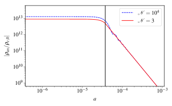
where (see Fig. 1). If , then the field is overdamped and does not oscillate.
To state the EFA for perturbations, it is helpful to rewrite the ULA’s exact equations of motion in terms of synchronous gauge fluid variables to obtain Hložek et al. (2015)
| (7) | ||||
| (8) | ||||
| (9) | ||||
| (10) |
with , , , and . Note that these equations with fluid variables are still exact, and equivalent to Eqs. (1)-(2) with field variables ). This formulation is the generalized dark matter (GDM) formulation of Ref. Hu (1998).
The oscillations at frequency can be removed from Eq. (7) by using the fact that the ULA fluid equations are well described by an effective fluid with cycle-averaged and which are not oscillating with the ULA field. We have already seen that when , implying that the cycle-averaged .
Applying the ansatz , the authors of Ref. Hwang and Noh (2009) find the cycle-averaged sound speed to be
| (11) |
where and are the cycle-averaged ULA pressure and density fluctuations in the ULA’s cycle-averaged rest frame.
Using more general assumptions about equipartition between kinetic and potential terms (and without assumptions about the functional form of scalar-field oscillations), the same expression for the cycle average of is derived in Ref. Poulin et al. (2018a), and generalized to potentials of the form near their minimum, where and the field rapidly oscillates. Scalar fields described by such potentials are one way of resolving the tension between CMB data and more local measurements of , by way of an era of early dark-energy (EDE) dominance Poulin et al. (2018b); Agrawal et al. (2019); Lin et al. (2019); Smith et al. (2019).
For , the hierarchy of timescales between scalar-field oscillation and the Hubble parameter is far less extreme, and the perturbed Klein-Gordon equation may be solved exactly in the course of an MCMC simulation Poulin et al. (2018a); Agrawal et al. (2019). The relative impact of anharmonic terms and a fluid approximation on observables and constraints in EDE models is the subject of ongoing discussion Poulin et al. (2018b); Agrawal et al. (2019); Lin et al. (2019); Smith et al. (2019).
Substituting and into Eqs. (8)-(9), we arrive at a set of effective (cycle averaged) equations of motion for the ULA fluid variables that are valid when . These define the EFA:111The expressions in Refs. Hložek et al. (2015); Poulin et al. (2018a) have additional terms in both perturbed fluid equations due to the transformation from the comoving gauge where is derived to the synchronous gauge usually used in CMB calculations. It was verified there (and confirmed here) that these terms are negligible compared to those shown and do not affect any of the conclusions of this paper.
| (12) | ||||
| (13) | ||||
| (14) |
The term proportional to in Eq. (14) is the linear-theory expansion of the quantum pressure term discussed in the fuzzy dark matter and ULA literature.
The EFA is only valid once the field (or perturbation modes) begins to coherently oscillate, and so the exact field equations must be solved at early times, with a switch implemented from exact to cycle-averaged equations when , where is a constant that defines a specific EFA implementation. The ULA fluid variables , , and are matched to ensure continuity at the switch.
II.3 Alternative cycle-averaging procedure
In Ref. Ureña López and Gonzalez-Morales (2016), a different set of variables is used for mode evolution. Dimensionless angular coordinates , are defined in lieu of and , along with their difference . Coherent oscillation (at times for which ) is explicitly built into the formalism through terms like and . At early times, the resulting equations are equivalent to the exact field equations [Eqs. (1) and (2)], and thus to our early-time GDM equations. At late times, these equations are stiff and an exact integration is still numerically intractable for use in fast cosmological parameter-space exploration. Some cycle-averaging procedure is thus still needed there.
To that end, an alternative cycle-averaging procedure is introduced in Ref. Ureña López and Gonzalez-Morales (2016). Oscillatory functions (, , or , depending on the equation) are replaced with
| (15) |
for (where ). When , is numerically set to zero. For example, the replacement
| (16) |
is made.
Put simply, a smoothed switch is used to separate the fast () and slow () timescales for ULA evolution. The chosen smoothing width is very narrow (), and thus qualitatively is likely to still exhibit whatever undesirable transient behavior occurs in the EFA discussed above.
Since , at times , the equations evolved in Ref. Ureña López and Gonzalez-Morales (2016) are effectively
| (17) | ||||
| (18) | ||||
| (19) |
where [noting that ]
| (20) | ||||
Note the natural appearance of the ULA Jeans wave number .
Differentiating Eq. (20) using Eqs. (18) and (19), we can represent the equations of motion for the variables and in terms of more standard fluid variables, yielding
| (21) | ||||
| (22) | ||||
| (23) |
Equation (21) is just Eq (12) in the limit valid at late times. Equation (22) is Eq. (13) if the term on the right-hand side of Eq. (13) is dropped. Finally, Eq. (23) is Eq. (14) in the nonrelativistic limit of Eq. (11) that . We verify in Appendix B that these differences are numerically irrelevant for CMB observables, and so the method of Ref. Ureña López and Gonzalez-Morales (2016) is equivalent to the EFA.
II.4 EFA implementation summary
The choice was used to obtain constraints on ULAs in Refs. Hložek et al. (2015, 2018). In this work, we investigate the accuracy of the EFA implementation as well as that of two other approaches. In one, the switch is imposed when (as in Ref. Poulin et al. (2018a)), which is also when . In the other EFA implementation (see Sec. II.3 and Ref. Ureña López and Gonzalez-Morales (2016)), the switch is imposed when . This is equivalent (if the transition occurs during radiation domination) to , and so we use that notation for the remainder of this work.
For the “exact” case, we solve the full KG field evolution [Eqs. (1) and (2)] until and then switch to an (extremely) late-time EFA. This is done as the logarithmic conformal time step needed to resolve rapid oscillations becomes prohibitively small for efficient computation at late times. For all but the largest mass considered ( eV), the switch to the EFA occurs after recombination. The predicted CMB anisotropies thus accurately reflect the impact of exact scalar-field dynamics, though we expand on this issue further in Sec. V.
We summarize the various implementations in Table 1. For the range under consideration here, we note that computing a full set of CMB power spectra for the “exact” case is an order of magnitude more computationally expensive than the , or implementations.
III Boltzmann code
In order to investigate the effect of the EFA, we developed a Python Boltzmann code to calculate individual mode growth, CMB anisotropy power spectra, and the matter power spectrum in the presence of ULAs. We use our own Boltzmann code (as opposed to modifying existing codes such as CLASS Blas et al. (2011) or CAMB Lewis (2000)). We do this to clearly isolate the effect of different treatments of ULA perturbations (treated with sufficient time resolution) without requiring extensive modification to these more complete Boltzmann codes to resolve such time cales. Some preliminary comparisons were made in Refs. Hložek et al. (2015); Poulin et al. (2018a), but without assessing implications for parameter inference.
In our code, the other components of the universe (dark matter, baryons, radiation, neutrinos, dark energy) are evolved using the equations from Ref. Ma and Bertschinger (1995), and we compute CMB power spectra using the line-of-sight method Seljak and Zaldarriaga (1996). We keep seven photon modes and neutrino modes, and we truncate the hierarchy of equations as in Ref. Ma and Bertschinger (1995). We use the initial conditions for a universe with ULAs as derived in Refs. Hložek et al. (2015, 2018) (using methods also applied in Ref. Doran et al. (2003); Shaw and Lewis (2010); Chluba and Grin (2013)).
We ported a public C++ implementation of the RECFAST code Seager et al. (2000, 1999); Chluba and Thomas (2011); Seager et al. (2011) into Python, in order to compute cosmic recombination histories with reasonable precision. It is known that a variety of additional physical effects (beyond those included in the multi-evel atom computation underlying RECFAST) affects recombination at the level (e.g. higher- two-photon transitions, resonant scattering in the Lyman-, deviations from statistical equilibrium between angular momentum substates of high- Rydberg states). These and other recombination effects are discussed in Refs. Chluba and Sunyaev (2008, 2007); Hirata (2008); Chluba and Sunyaev (2009a); Grin and Hirata (2010); Chluba and Sunyaev (2009b); Hirata and Forbes (2009); Ali-Haimoud and Hirata (2010); Ali-Haimoud et al. (2010); Ali-Haimoud and Hirata (2011); Kholupenko et al. (2010, 2011) (and references therein).
We implemented the numerical methods used in Ref. Callin (2006), and have neglected neutrino mass. Current CMB data are consistent with this choice Gil-Botella (2013) (though neutrino experiments indicate a nonzero neutrino mass whose absolute scale could be detected by future CMB experiments Abazajian et al. (2016)), allowing us to avoid the complications of following perturbation evolution in a species that transitions from relativistic to nonrelativistic on cosmological timescales Lewis and Challinor (2002); Shaw and Lewis (2010); Blas et al. (2011); Lesgourgues and Tram (2011). We neglect smoothing of primary CMB anisotropies by weak gravitational lensing. We include homogeneous reionization as in Ref. Lewis (2013).
ULAs are added self-consistently as described in Sec. II.1. We use the SciPy Virtanen et al. (2019) ODE solver with vode Brown et al. (1989) integrator using a bdf (stiff) method. Rather than stepping forward using derivatives computed at present-day function values, this implicit technique solves nonlinear equations for future function values, using expressions which approximate the relevant derivatives in terms of future and present function values. Implicit techniques are well suited to stiff differential equations – the system under study here has two vastly disparate timescales [ and ], making it well suited to the chosen numerical method. We set a large () maximum number of steps. The most important parameters are the relative and absolute error tolerance parameters, which are set to values of and , respectively.
When plotting spectra, we set all the parameters except the ULA mass and ULA dark matter fraction to their best fit values from the 2015 Planck data release Ade et al. (2016a).222While this work was nearing completion, the Planck 2018 results were released Aghanim et al. (2018). Because of the very small shifts in central values of parameters between the 2015 and 2018 Aghanim et al. (2018) data releases, and very weak dependence of bias results on fiducial parameter values over the allowed range, our conclusions should be unaffected by the difference between the two iterations of Planck results. In Sec. V, we explore variations in all cosmological parameters when assessing the impact of the EFA on ULA parameter inferences.
Note that cold dark matter makes up a fraction of the energy density . We consider only ULA masses eV. This mass restriction guarantees that ULAs begin to dilute as matter () before matter-radiation equality (“equality” henceforth) Hložek et al. (2015), keeping us in the “DM-like” part of ULA parameter space. We will explore the impact of the EFA in the “DE-like” part of the mass range () in future work. As initial conditions for the homogeneous axion field , we use and Marsh (2016).
We use a root-finding algorithm interfaced with our homogeneous scalar-field evolution module to find the value of which reproduces the desired value of . The initial guess is chosen to be , where is defined as the scale factor when , with computed using CDM to obtain an initial guess but self-consistently including ULAs thenceforth. The algorithm assumes the existence of a root in the range , which we have confirmed is sufficient for all values of the parameters explored in this work. For the perturbations, adiabatic initial conditions give Marsh (2016); Hložek et al. (2015), and, because of large Hubble drag initially, Poulin et al. (2018a).
Our CMB and matter power spectrum in the absence of ULAs were compared against CAMB Lewis (2000) with quantitative agreement at the level, except for , where agreement is at the level for the EE angular power spectrum and for the TT power spectrum . Although there is a difference between the code used in this work and CAMB, it is unimportant because our goal here is a comparison between the “exact” treatment and the EFA with all other assumptions and computational tools held fixed for self-consistency. Our use of a simplified, relatively accurate recombination history (and simplifying approximations for neutrinos, as described above) should be sufficient for this goal.
IV Mode growth and CMB
We now explore the impact of the various EFA implementations on cosmological observables. Naively, one might expect that later switches (by following the exact EOMs for longer) would always perform better, but this is not the case, as we explain below.
IV.1 Mode evolution
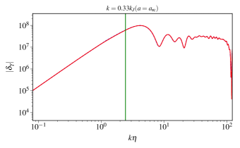
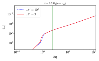
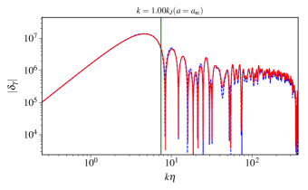
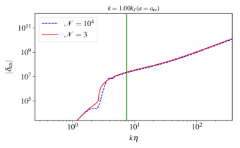
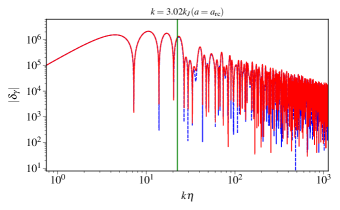
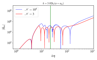
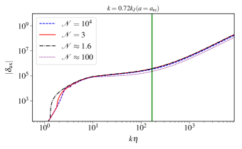
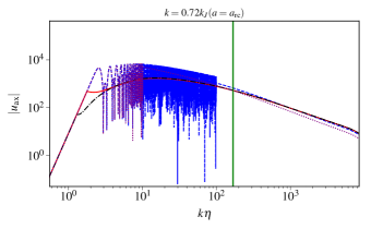
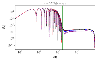
We first study the effect of the EFA on the growth of individual modes. To understand general features, we show individual mode growth for different values of in Fig. 2. We show the evolution of given our obvious interest in its dynamics and of , as it is the fluid variable most important for observed properties of the CMB. A useful reference scale is given by the comoving ULA Jeans wave number
| (24) |
Modes with have suppressed growth relative to CDM, as the perturbation lies within the ULAs wavelength Nambu and Sasaki (1990). We expect that (where is the scale factor at recombination) will be the important scale for computations of CMB anisotropies. We find using the peak of the visibility function with with being the density of electrons and the Thomson cross section.
For , the approximation and the “exact” treatment agree asymptotically, so there is only a small change in the photon overdensity, . Once , there are noticeable differences between the two approaches, as seen both in the ULA overdensity and in , which could have an observable impact on CMB anisotropy measurements. Although we show mode evolution for eV, the qualitative features hold for other values.
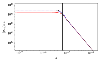
We compare all three EFA implementations with the “exact” calculation in Fig. 3, for the value . We see that the implementation captures early-time homogeneous density evolution more accurately than the implementation, as well as early-time perturbation evolution (at least for the mode shown). This is unsurprising given that this implementation follows the exact scalar-field EOMs for a much larger number of oscillation cycles. The implementation captures the later-time evolution of both ULA and photon variables more accurately, as there is more time for numerical transients (introduced by a discontinuous swap in the second derivatives of various fluid quantities) to dissipate. Given the differences between perturbation evolution in different implementations, a more detailed comparison of CMB power spectra is necessary.
IV.2 CMB anisotropies
We now compute CMB anisotropies for our full grid of models using the standard line-of-sight formalism as implemented in Sec. III. The ordering of the accuracy of different EFA implementations depends on the mass. The WKB approximation underlying the EFA is itself an expansion in the small (time-dependent) parameter , which might be taken to imply that the implementation should always outperform the implementation, but this is not the case. Why?
All of these implementations excite spurious transients near the time of transition from the exact KG to EFA equations. The higher- cases also have later switches, leaving less time for transient behavior to dissipate before recombination. There is thus a delicate balance at play (between suppression of transients and formal convergence of the WKB approximation) in determining which version of the EFA is best. This balance depends on when the switch occurs compared to the evolution of the observed CMB fluctuation modes, and is thus sensitive to both and .
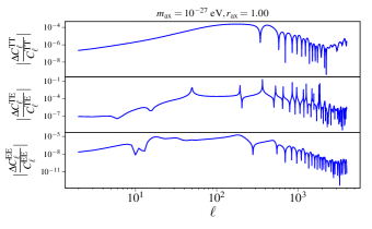
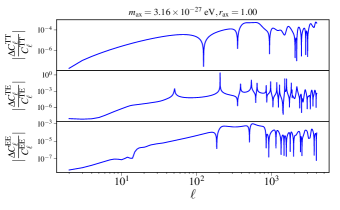
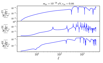
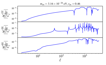
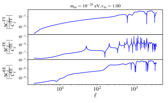
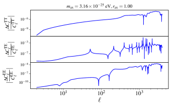
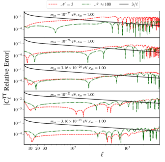
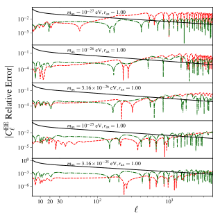
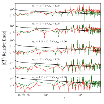
For the and implementations, we show the primary TT, EE, and TE () power spectra for and in Fig. 4. This value of is not allowed by the constraints Hložek et al. (2015, 2017), but is chosen to visually accentuate differences between approaches. We also show relative errors between different EFA implementations. In addition to the individual , we plot fiducial model points with error bars corresponding to cosmic variance. Following Ref. Ade et al. (2016a), the modes are binned into bins of sizes for in the range , respectively. The value plotted is the weighted average of with cosmic variance error at the weighted average with weight proportional to , as in the Planck Collaboration pipeline Aghanim et al. (2016). For a variety of other values, we explore the relative accuracy of different EFA implementations in Appendix 16 using Fig. 16.
For , the implementation is less accurate than the implementation for TT and EE spectra, and comparable for TE. For , the and implementations are of comparable accuracy (compared with the exact KG equation) at most values. For , the implementation is more accurate than the implementation.
Similar comparisons can be made for the implementation, whose performance relative to other choices is a function of . At higher values, the residuals are in between those of the and implementations, while at lower values, the residuals are worse than any of the other implementations. In the interests of simplifying the discussion, we have omitted these results from figures showing power-spectra comparisons but include it in our final computations of bias in ULA density constraints.
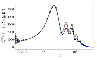
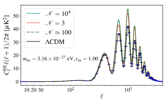
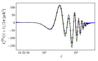
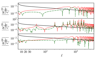
Depending on the implementation and value, the fractional error can be several orders of magnitude in excess of the approximate Planck noise level () when . Forthcoming experiments (e.g. CMB-S4 Abazajian et al. (2019)) will measure nearly perturbation modes. Roughly speaking Shimon et al. (2013), the fractional effect of any systematic error in the computation of CMB anisotropies grows as , where is the total number of multipole values with . Small biases thus require that , with detailed numerical considerations yielding the useful rule of thumb that bias-free parameter inference requires Seljak et al. (2003); Shimon et al. (2013, 2012). We see in Figs. 4 and 16 that this condition is violated by several orders of magnitude at high when .
As and , it stands to reason that the fractional error between all three EFA implementations and the “exact” calculation exceeds the needed accuracy for unbiased parameter inference, depending on the detailed full structure of the likelihood function (e.g. parameter degeneracies). To determine if the errors induced by the EFA significantly affect cosmological constraints to (or measurements of) ULA DM, we must compare the scale-dependent error with the information content of the CMB, as represented by the Fisher matrix Tegmark et al. (1997); Bond et al. (1997); Eisenstein et al. (1999). We now estimate the EFA-induced parameter bias.
V statistic and bias
We wish to estimate the systematic error in CMB measurements of (or limits on) the axion relic density from the CMB that results from the use of the EFA. Although a full analysis would require mock datasets and MCMC analysis, reasonable estimates may be obtained using standard Fisher-analysis techniques Tegmark et al. (1997); Bond et al. (1997); Eisenstein et al. (1999).
The elements of the Fisher matrix for the CMB anisotropy power spectrum are given by Tegmark et al. (1997); Kamionkowski et al. (1997); Shimon et al. (2013):
| (25) |
where is a choice of CDM parameters, along with the ULA density of today, and is the sky fraction covered by the CMB experiment of interest. Here the data covariance matrix is . The brackets denote an ensemble average and is the usual optimal estimator of angular power spectra using the multipole moments as data, where the observable consists of the pair . We neglect -mode (curl) anisotropies here, as our analysis neglects weak gravitational lensing of the CMB and primordial tensor modes.
The ULA mass is varied and the full Fisher matrix with elements is recomputed at each value, to see how biases and parameter errors depend on ULA mass. The derivative quantifies the response of the observables to the CDM and ULA parameters of interest; typically this derivative must be obtained numerically using a Boltzmann code, though for , the derivative may be obtained analytically (). If we compute the Fisher matrix for a theoretical scenario and some experiment, we may forecast the error on the best fit parameters via , assuming that the parameter likelihood (given the data) distribution is Gaussian.
The elements of the data covariance matrix are Kamionkowski et al. (1997); Knox (1995)
| (26) | ||||
where is the noise power spectrum for the observable . The remaining elements follow trivially since . The above covariance matrix takes into account both the cosmic variance, and the noise of the detector Kamionkowski et al. (1997). We use the usual approximations of Ref. Knox (1995), with an overall amplitude noise amplitude in . The instrument beam is assumed to be Gaussian with a full-width half-max angular size of in radians.
The errors in the theoretical calculation of drive the peak of the likelihood to a different set of parameter values than the true model parameters, resulting in parameter biases. Under a Gaussian likelihood approximation, we follow Refs. Knox et al. (1998); Santos et al. (2003); Zahn et al. (2005); Taburet et al. (2008); Shimon et al. (2013, 2012) to compute this bias, which is Taburet et al. (2008)
| (27) |
where
| (28) |
and is the shift in computed theoretical power spectra between the “exact” treatment of ULAs and the EFA.333We follow Refs. Knox et al. (1998); Santos et al. (2003); Zahn et al. (2005); Shimon et al. (2013, 2012) and drop higher-order terms of order in the Fisher matrix itself, as these lead to corrections of the form to the bias. These terms are subdominant unless there is a ULA detection of high significance. This expression takes into full account degeneracies between different cosmological parameters. If the bias in resulting from use of the EFA can be absorbed by adjusting other cosmological parameters, Eq. (28) will indicate a negligible shift.
In the future, if other measurements (e.g. large-scale structure surveys or the CMB weak lensing trispectrum) are combined with CMB power spectrum measurements (dominated by primary anisotropies) to break parameter degeneracies, a larger bias may result. The bias and error in with all other cosmological parameters held fixed are given by
| (29) | ||||
| (30) |
Before computing an extensive set of numerical derivatives, it would be useful to establish the maximum bias on a single parameter, normalized to its Fisher-level error. Using Eq. (29) and the Cauchy-Schwarz inequality (see Appendix C for a derivation), it can be shown that
| (31) |
This statistic Hirata has been used to estimate the impact of improvements to cosmic recombination history computations on CMB parameter estimation Hirata (2008); Hirata and Forbes (2009); Grin and Hirata (2010). If , we can safely conclude that the systematic errors in induced by use of the EFA make a negligible impact on the estimation of both and standard cosmological parameters. Conversely, if , there could be large shifts in central values, and a bias estimate computed using Eq. (28) or (29) is needed.444 is just the square root of the predicted change in the statistic induced by the use of the EFA. The interpretation of as the maximum fractional bias in a single parameter (neglecting degeneracies) requires the added assumption of a Gaussian likelihood for the parameters.
V.1 Z-statistic for current and future CMB experiments
We compute the Z statistic using Eqs. (26) and (31), assuming noise properties for various CMB instruments (past, present, anticipated) given in Table 2. Of course even an ideal zero-noise experiment is affected by cosmic variance and is shown as the cosmic-variance limited (CVL) case. In this case, quantifies the maximum impact of EFA-induced errors on CMB constraints to .
| Experiment | FWHM | Noise | Ref. | ||
|---|---|---|---|---|---|
| WMAP V band | 21 | 434 | 0.65 | 2200 | Ref. wma (2014) |
| WMAP W band | 13 | 409 | 0.65 | 2200 | Ref. wma (2014) |
| Planck 143 GHz | 7.1 | (37, 78) | 0.65 | 2200 | Ref. Ade et al. (2013) |
| Planck 217 GHz | 5.0 | (54, 119) | 0.65 | 2200 | Ref. Ade et al. (2013) |
| ACTPol | 1.4 | 8.9 | 0.097 | 2200 | Ref. Niemack et al. (2010) |
| SPT-3G | 1.1 | 2.5 | 0.06 | 2200 | Ref. Crawford (2014) |
| CMB-S4 | 3.0 | 1.0 | 0.50 | 2200 | Ref. Abazajian et al. (2013) |
| CVL | 0.0 | 0.0 | 1.0 | 2200 |
We create a 7 X 7 logarithmically spaced grid with eV eV and , and evaluate the statistic for the three different versions of the EFA. For temperature, we restrict ourselves to , as secondary temperature anisotropies dominate the primordial CMB at smaller scales (although there are futuristic proposals to go well beyond this limit, e.g. Refs. Nguyen et al. (2017); Sehgal et al. (2019)). Since polarization foregrounds are expected to be less severe (than ones in the temperature) at small angular scales Abazajian et al. (2016), we assume for polarization data and use the similar (polarization-only) expression
| (32) |
with .
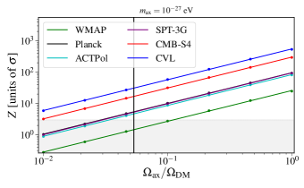
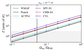
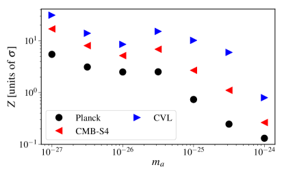
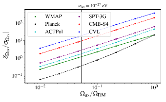
As an example, in Fig. 5, we show the statistic as a function of for , where the constraints of Ref. Hložek et al. (2015) are most stringent, and where the effects of the EFA are most severe. If the true ULA abundance saturates current constraints (from the CMB power spectra without lensing, as in Ref. Hložek et al. (2015)), we see that (depending on the experiment), the bound indicates potential biases as large as . The effect is significantly less pronounced if only temperature data are used, highlighting the importance of CMB polarization. If the actual ULA density is far lower than present-day constraints, could be much smaller, allowing the EFA-induced error to be neglected.
To succinctly capture the potential impact of the EFA (for the implementation) at all masses, we plot for values saturating the constraints of Ref. Hložek et al. (2015) in Fig. 6, including temperature and polarization anisotropies. We see that for , and greater biases could occur for all three experimental scenarios considered there. For CMB-S4 or the CVL case, significant () values occur for values as high as . We also compute for the and implementations. These results are of the same order of magnitude, and are thus omitted for brevity.
To check that the constraints of Ref. Hložek et al. (2015) are robust and to assess the impact of the EFA on future CMB tests of ULA physics, we must thus evaluate the more complete Fisher-matrix based estimates [Eqs. (28) and (29)]. These are needed to properly include the detailed response of to variations in all implementations considered, and to properly assess the impact of parameter degeneracies.
V.2 Bias
Since the statistic was for a significant part of parameter space, we directly compute the bias in the value of induced by the use of the EFA. We compute the parameter bias for our full 7 X 7 grid of models using Eq. (28) and forecast the error on the best fit parameters via . As noted in Sec. V.1, for we expect temperature measurements to be dominated by secondary anisotropies, and restrict all Fisher sums to EE-only portions of the data covariance matrix.
We calculate the relevant numerical derivatives with respect to CDM parameters by modifying the Planck values at the percent level as in Ref. Eisenstein et al. (1999) and using the two-point symmetric finite difference method. We also compute derivatives with respect to . These bias/error estimates are thus a first-order approximation, given the use of for derivatives with respect to CDM parameters.
For the derivative with respect to , we check convergence by comparing the two-point symmetric, left, and right finite-difference methods and verifying that the bias is converged at the level for , where ULA sensitivity is very poor and the overall bias . Below, we discuss how large the bias would be for values saturating current constraints, but note that the bias will be less severe for values well below the current upper limits. We confirm for the null (no ULA) hypothesis that Planck parameter error levels are reproduced. For the implementation, we also confirm that if ULAs are included that the marginalized curve (as a function of ) is consistent (at order-of-magnitude level) with the constraints of Ref. Hložek et al. (2015), which were obtained using the same EFA implementation.
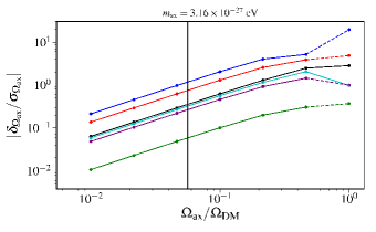
We begin by focusing our attention on the fiducial case. As an example, in Fig. 7, we show the bias for using hypothetical temperature and polarization data, as a function of . We see that for this value, the bias is negligible for values satisfying the constraints of Ref. Hložek et al. (2015). As beam, noise, and are varied, different scales are emphasized in the calculation of bias, and so it is natural that there is some nonmonotonicity with respect to experimental ordering and . Additionally, the bias can be positive or negative depending on the subtle interplay of some of these parameters.
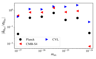
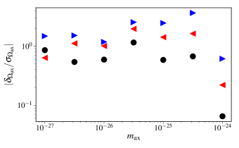
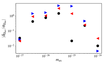
To better capture the information content of all these bias figures, we tabulate the dimensionless bias as a function of , with fixed at the current constraint level (at that value). The results (for Planck, CMB-S4, and the CVL case) are shown in Fig. 8. We see that small biases () in ULA densities occur at Planck noise levels. The CMB-only results of Ref. Hložek et al. (2015) are thus robust to the use of the EFA for . For more futuristic noise levels (e.g., the CMB-S4 and CVL cases), the bias for the primary CMB remains relatively small () in the range shown.
Our reference case for all this analysis is the “exact” case, which in actuality still has a switch to the EFA at very late times (when ), long after recombination at all values where the primary CMB significantly constrains . Qualitatively, then, we expect that any transients in mode evolution introduced by the use of this switch will not alter our results. To test this expectation, we repeated all the bias analysis with the restriction that , where is the angular size of the causal horizon when , and found that the conclusions implied by Fig. 8 are unaffected by the late-time switch.
So far, our estimates of bias have been computed using Eq. (28), and these include parameter degeneracies (between ULAs and standard cosmological parameters). We may alternatively treat standard cosmological parameters as fixed and neglect parameter degeneracies, using Eq. (29) to compute the bias at maximum-likelihood parameter values. These results will be an upper bound to the absolute value of the bias when complementary datasets (e.g galaxy clustering or weak lensing, or CMB lensing) are used to break degeneracies. A complete treatment of this issue requires a combined Fisher analysis for CMB power spectra and other data, but we leave this for future work. To evaluate in Eq. (29), we use the relation , valid for the variance of with a multivariate Gaussian likelihood, if other parameters are held fixed.
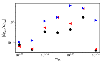
As an example, in Fig. 9, we show the bias for using hypothetical temperature + polarization data, as a function of . We see that or greater biases result at SPT-3G & CMB-S4 noise levels, as well as in the CVL case. Biases are smaller than for the ACTPol, WMAP, and Planck cases.
One important aspect of the bias (see above) is that better experiments do not necessarily have larger magnitude bias, and that the bias can be positive or negative. We have verified that this occurs because and can have different signs, and as a result, the terms in the bias sum can have either sign. In the case of Fig. 9, on the scales that WMAP most accurately probes, the terms almost all have the same sign, but, when adding more accurate high- Planck measurements, added terms with opposite signs reduce the bias amplitude. More precise (current and future) experiments reach even deeper into this high- regime, causing the amplitude of the fractional bias to retain its sign but increase in amplitude.
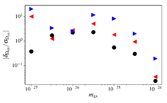
In Fig. 10, we show the dimensionless bias (now neglecting degeneracies), as a function of , with fixed exactly at the current constraint level. As in some of the cases above, the sharp dip in the CVL bias at (from which the bias curve returns to a more standard ordering) is driven by physical sign changes in the summand of Eq. (29). We see that at some of the most constrained masses, (), large biases () in ULA densities occur at Planck noise levels.
For more futuristic noise levels (as shown by the CMB-S4 and CVL cases), similar and even larger biases result if . We note Fisher-matrix calculations that indicate biases greater than several should just be taken as an indication that the actual bias is severe and not a precise result, given the breakdown of the Gaussian likelihood approximation for large deviations from central values.
We see that biases are large when parameters are fixed, but not when they are marginalized over; this implies that the systematic errors in values induced by the EFA are significantly degenerate with shifts in other cosmological parameters. It is natural to wonder then, if future more precise measurements of standard cosmological parameters will push bias toward the larger values shown in Fig. 10.
We explored this issue further using forecasts for matter power spectrum measurements by the Large Synoptic Survey Telescope (LSST) Zhan and Tyson (2018), Dark Energy Spectroscopic Instrument (DESI) Casas et al. (2017), Euclid satellite Casas et al. (2017); Sartoris et al. (2016), and Square Kilometer Area (SKA) Bacon et al. (2018), as well as more direct distance ladder-based/gravitational-wave inferred measurements of the Hubble constant Beaton et al. (2019). We imposed priors to cosmological parameters via a diagonal modification to the Fisher matrix, , where is the forecasted error to a CDM parameter from one of these efforts (priors were applied to , , , and as appropriate given Refs. Zhan and Tyson (2018); Casas et al. (2017); Sartoris et al. (2016); Bacon et al. (2018); Beaton et al. (2019)).
We then used Eq. (27) to compute the bias to resulting from the use of the EFA in the presence of priors, and found in all cases that the results reproduced those of Fig. 8 at the level, and were not comparable to the large bias in Fig. 10. In other words, the primary CMB Fisher matrix exhibits sufficient parameter degeneracy for the impact of the EFA on ULA parameters to be absorbed by variations in other parameters, even in the presence of sensible priors from upcoming experiments. Future work to extend this analysis should include CMB lensing and the full off-diagonal Fisher matrices from galaxy surveys (and other efforts), including the impact of ULAs on galaxy and cosmic shear clustering power spectra.
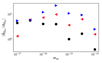
We also evaluated bias with no priors for the and implementations, and show the results in Figs. 11-14. At Planck noise levels for the implementation, for all values if we marginalize over cosmological parameters (see Fig. 11). For the CVL case here, . If cosmological parameters are fixed, the bias in the CVL case is large: (see Fig. 12).
For the implementation at Planck noise levels including cosmological parameter marginalization, , while if cosmological parameters are assumed fixed, at the same noise level (see Fig. 13). For the CVL case with cosmological parameter marginalization if and otherwise. For the implementation with cosmological parameters held fixed in the CVL case, if and otherwise.
We note that the implementation exhibits an unusual property in the nonmarginalized bias computation [see Eq. (29) and Fig. 14]. Unlike the and implementations (see Figs. 10 and 12), the low single-parameter bias computed in the implementation is far smaller than the bound implied by the order of magnitude of (see Fig. 6), i.e. . The dimensionless bias in this case [Eq. (29] is essentially a dot product between the vectors and , under a metric set by the data covariance.
As discussed in Appendix C, the Cauchy-Schwarz inequality thus imposes the bound , but does not require the bias to saturate this bound. Examining the summand of this dot product, we note that the implementation yields values that oscillate about zero with alternating sign, compared with the & implementations, which typically show a negative semidefinite offset () at values that contribute significantly to the sum. This sign structure appears to be responsible for the single-parameter behavior of the implementation. The implementation also exhibits a different ordering of single and multiparameter (degenerate) bias levels at some masses than the other implementations, likely due to the different covariance level of with in the Fisher matrix in the implementation.
VI Conclusions
In this work, we have quantitatively compared predictions for cosmological observables in ultra-light axion (ULA) models obtained from the effective fluid approximation (EFA) with the results of a full Klein-Gordon (KG) treatment of the dynamics. Along the way, we found that an alternative treatment of ULA perturbations Ureña López and Gonzalez-Morales (2016) is, in fact, equivalent to the EFA, when written in terms of appropriate variables; in future work, it would be valuable to undertake a more systematic comparison of our methods.
We forecasted the resulting bias to ULA parameters from primary (unlensed) CMB anisotropy power spectrum measurements, using well-established Fisher-matrix techniques to estimate how the numerical discrepancies between EFA and KG predictions will offset the centroids of the parameter likelihood, assuming that a ULA detection is hiding just underneath the sensitivity level of completed experimental analyses.
For the version of the EFA, we find that if the full field dynamics are neglected, primary CMB anisotropy constraints to ULAs from Planck are robust, while constraints to/measurements of from future CMB experiments (e.g. CMB-S4 Abazajian et al. (2019)) will be moderately biased at the level, if marginalization over the usual cosmological parameters is assumed. If an idealistic external dataset can break all the relevant degeneracies, the bias could be as high as . We find that no immediately planned effort will approach this bias level.
These conclusions could be altered when the full covariance matrix of future large-scale structure efforts (including degeneracies among standard cosmological parameters and their covariance with ULA parameters) is used, and we will address this issue in future work. For the and implementations in the marginalized case, we find comparable (but slightly worse, by a factor of ) bias levels when cosmological parameters are marginalized over.
It is interesting to note that the fractional differences between the different choices of - which generate residuals well in excess of the threshold - lead to relatively small biases at least, in part, because the residuals have support over a large range of . On the other hand, it stands to reason that if the residuals were more localized in we might have found a much larger bias (as recently pointed out in a different context in Ref. Smith et al. (2019)).
Measurements of CMB weak lensing are a key scientific driver for upcoming experiments like CMB-S4 Abazajian et al. (2019) or more futuristic ideas like CMB-HD Nguyen et al. (2017). These efforts have the promise of sensitivity to ULAs in the window , where they might comprise all the DM. In future work, we will thus extend our work to include measurements of the lensing potential power spectrum and higher values. The EFA generally works best at late times (where the lensing kernel peaks Hanson et al. (2010)), but it is also possible that the large information content of the full CMB -point correlation function (which drives constraints to the lensing potential power spectrum Hanson et al. (2010)) induces larger biases.
The tools used in this work to compute observables for the “exact” computational benchmark only solve the Klein-Gordon equation until , which is more than sufficient for the time and length scales probed by primary CMB anisotropies (as discussed in Sec. V.2). Future work will require us to extend the “exact” case to later times, in order to conduct definitive comparisons with the EFA in the case of CMB lensing, and other observables sensitive to the matter power spectrum (e.g. the galaxy correlation and shear power spectra to be probed with exquisite accuracy by LSST Abell et al. (2009) and other comparable efforts).
In this work, we have assumed purely adiabatic initial conditions. If the relevant global symmetry is broken before the end of the inflationary era, the ULA field (as a nearly massless scalar spectator) will carry quantum fluctuations with , where is the Hubble expansion rate during inflation. These fluctuations will in turn source primordial DM isocurvature (entropy) fluctuations (See Refs. Hložek et al. (2018) and references therein). These are observationally known to be subdominant Ade et al. (2016b) (while still allowing large values), but could be detected by ongoing/upcoming CMB experimental efforts Abazajian et al. (2019).
The CMB will thus provide interesting constraints to and , complementing the impact of CMB polarization-based tests of the inflationary tensor-to-scalar ratio . Entropy fluctuations are more directly sensitive to dark-sector fluctuations than the adiabatic CMB power spectrum, and it is thus important to fully evaluate the EFA-induced bias in ULA isocurvature scenarios.
Acknowledgements.
T. L. S. and D. G. acknowledge support in part by NASA grant 80NSSC18K0728. D. G. and T. C. acknowledge support from the Provost’s office at Haverford College. T. C. thanks Haverford College for hospitality during the completion of this work. T. L. S. acknowledges support from the Provost’s office at Swarthmore College. This work was supported in part by the National Science Foundation under Grant No. NSF PHY-1125915 at the Kavli Institute for Theoretical Physics (KITP) at UC Santa Barbara. We thank A. Aoki, R. Hložek, W. Hu, L. Hui, M. Kamionkowski, D. J. E. Marsh, C. Owen, V. Poulin, and M. Raveri for useful conversations. D. G. thanks KITP for its hospitality during the completion of this work.Appendix A WKB
Recall that for the ULA background, we want to solve
| (33) |
Substituting , we find a differential equation solvable with the WKB method (see, for example, Ref. Bender and Orszag (2013)). It has the solution,
| (34) | ||||
with . Self-consistently, if , then we assume which implies , so we can assert . Then, the usual ansatz for the ULA field is recovered for some constant and . It then immediately follows that to leading order in .
Appendix B Alternative cycle averaging procedures
We note that our implementation of the implementation [which applies a switch with equations of motion (EOMs) given by Eqs. (7)-(9), a approximation, and the cycle-averaged sound speed, Eq. (11)] has additional gauge terms coming from the transformation from the fluid rest frame to the synchronous gauge. These terms are not present in Eqs. (21)-(23), which represent the formalism of Ref. Ureña López and Gonzalez-Morales (2016) in terms of fluid variables.
There are also differences between our expression for the cycle-averaged sound speed [Eq. (11)], and the simpler expression obtained in Ref. Ureña López and Gonzalez-Morales (2016).
As a result of the scaling of various terms with , the first set of differences can only be large for (at superhorizon scales), while the difference between the two different cycle-averaged sound speeds only grows large when , deep in the Jeans-suppressed regime of perturbation evolution. To be sure that these implementation differences do not affect our conclusions, we wrote a modified code that exactly implemented Eqs. (21)-(23).
The resulting differences in observables are shown in Fig. 15. Fractional differences in power spectra between the different versions of the implementation are several orders of magnitude smaller than differences between it and other implementations at scales contributing to the sums in expressions for and . Our conclusions about the relative accuracies of different EFA implementations are thus robust.
Appendix C statistic derivation
We define the following inner product (which clearly satisfies the usual axioms),
| (35) |
where the components of are for and in any arbitrary order. The Cauchy-Schwarz inequality holds for , as it is an inner-product. If we consider a one parameter model (so that for the Fisher matrix), we see
| (36) | ||||
where we used Eqs. (28) and (31). Since , we see . If there are multiple parameters being varied for the calculation of , the explicit bound may not hold, but the statistic can still give an estimate of the dimensionless bias.
Appendix D Additional CMB power spectra
References
- Crites et al. (2015) A. T. Crites et al. (SPT), Astrophys. J. 805, 36 (2015), arXiv:1411.1042 [astro-ph.CO] .
- Louis et al. (2017) T. Louis et al. (ACTPol), JCAP 1706, 031 (2017), arXiv:1610.02360 [astro-ph.CO] .
- Akrami et al. (2018) Y. Akrami et al. (Planck), (2018), arXiv:1807.06205 [astro-ph.CO] .
- Aghanim et al. (2018) N. Aghanim et al. (Planck), (2018), arXiv:1807.06209 [astro-ph.CO] .
- Van Waerbeke et al. (2013) L. Van Waerbeke et al., Mon. Not. Roy. Astron. Soc. 433, 3373 (2013), arXiv:1303.1806 [astro-ph.CO] .
- Alam et al. (2017) S. Alam et al. (BOSS), Mon. Not. Roy. Astron. Soc. 470, 2617 (2017), arXiv:1607.03155 [astro-ph.CO] .
- Abbott et al. (2018a) T. M. C. Abbott et al. (DES), (2018a), arXiv:1810.02499 [astro-ph.CO] .
- Abbott et al. (2018b) T. M. C. Abbott et al. (DES), (2018b), arXiv:1811.02375 [astro-ph.CO] .
- Jones et al. (2018) D. O. Jones et al., Astrophys. J. 857, 51 (2018), arXiv:1710.00846 [astro-ph.CO] .
- Abbott et al. (2018c) T. M. C. Abbott et al. (DES), (2018c), arXiv:1811.02374 [astro-ph.CO] .
- Jungman et al. (1996) G. Jungman, M. Kamionkowski, and K. Griest, Phys. Rept. 267, 195 (1996), arXiv:hep-ph/9506380 [hep-ph] .
- Feng (2010) J. L. Feng, Ann. Rev. Astron. Astrophys. 48, 495 (2010), arXiv:1003.0904 [astro-ph.CO] .
- Peccei and Quinn (1977) R. D. Peccei and H. R. Quinn, Phys. Rev. Lett. 38, 1440 (1977), [,328(1977)].
- Wilczek (1978) F. Wilczek, Phys. Rev. Lett. 40, 279 (1978).
- Weinberg (1978) S. Weinberg, Phys. Rev. Lett. 40, 223 (1978).
- Kim (1979) J. E. Kim, Phys. Rev. Lett. 43, 103 (1979).
- Shifman et al. (1980) M. A. Shifman, A. I. Vainshtein, and V. I. Zakharov, Nucl. Phys. B166, 493 (1980).
- Zhitnitsky (1980) A. R. Zhitnitsky, Sov. J. Nucl. Phys. 31, 260 (1980), [Yad. Fiz.31,497(1980)].
- Dine et al. (1981) M. Dine, W. Fischler, and M. Srednicki, Phys. Lett. 104B, 199 (1981).
- Asztalos et al. (2006) S. J. Asztalos, L. J. Rosenberg, K. van Bibber, P. Sikivie, and K. Zioutas, Ann. Rev. Nucl. Part. Sci. 56, 293 (2006).
- Kim and Carosi (2010) J. E. Kim and G. Carosi, Rev. Mod. Phys. 82, 557 (2010), arXiv:0807.3125 [hep-ph] .
- Aprile et al. (2017) E. Aprile et al. (XENON), Phys. Rev. Lett. 119, 181301 (2017), arXiv:1705.06655 [astro-ph.CO] .
- Albert et al. (2017) A. Albert et al. (DES, Fermi-LAT), Astrophys. J. 834, 110 (2017), arXiv:1611.03184 [astro-ph.HE] .
- Hooper et al. (2017) D. Hooper, I. Cholis, T. Linden, and K. Fang, Phys. Rev. D96, 103013 (2017), arXiv:1702.08436 [astro-ph.HE] .
- Aad et al. (2014) G. Aad et al. (ATLAS), JHEP 09, 103 (2014), arXiv:1407.0603 [hep-ex] .
- Daylan et al. (2016) T. Daylan, D. P. Finkbeiner, D. Hooper, T. Linden, S. K. N. Portillo, N. L. Rodd, and T. R. Slatyer, Phys. Dark Univ. 12, 1 (2016), arXiv:1402.6703 [astro-ph.HE] .
- Du et al. (2018) N. Du et al. (ADMX), Phys. Rev. Lett. 120, 151301 (2018), arXiv:1804.05750 [hep-ex] .
- Vogel et al. (2013) J. K. Vogel et al., in 8th Patras Workshop on Axions, WIMPs and WISPs (AXION-WIMP 2012) Chicago, Illinois, July 18-22, 2012 (2013) arXiv:1302.3273 [physics.ins-det] .
- Caldwell et al. (2017) A. Caldwell, G. Dvali, B. Majorovits, A. Millar, G. Raffelt, J. Redondo, O. Reimann, F. Simon, and F. Steffen (MADMAX Working Group), Phys. Rev. Lett. 118, 091801 (2017), arXiv:1611.05865 [physics.ins-det] .
- Garcon et al. (2017) A. Garcon et al., (2017), 10.1088/2058-9565/aa9861, arXiv:1707.05312 [physics.ins-det] .
- Raffelt (2008) G. G. Raffelt, Axions: Theory, cosmology, and experimental searches. Proceedings, 1st Joint ILIAS-CERN-CAST axion training, Geneva, Switzerland, November 30-December 2, 2005, Lect. Notes Phys. 741, 51 (2008), [,51(2006)], arXiv:hep-ph/0611350 [hep-ph] .
- Cadamuro (2012) D. Cadamuro, Cosmological limits on axions and axion-like particles, Ph.D. thesis, Munich U. (2012), arXiv:1210.3196 [hep-ph] .
- Matos and Nieto (1993) T. Matos and J. A. Nieto, Rev. Mex. Fis. 39, S81 (1993).
- Frieman et al. (1995) J. A. Frieman, C. T. Hill, A. Stebbins, and I. Waga, Phys. Rev. Lett. 75, 2077 (1995), arXiv:astro-ph/9505060 [astro-ph] .
- Matos et al. (2000) T. Matos, F. S. Guzman, and L. A. Urena-Lopez, Class. Quant. Grav. 17, 1707 (2000), arXiv:astro-ph/9908152 [astro-ph] .
- Amendola and Barbieri (2006) L. Amendola and R. Barbieri, Phys. Lett. B642, 192 (2006), arXiv:hep-ph/0509257 [hep-ph] .
- Hu et al. (2000) W. Hu, R. Barkana, and A. Gruzinov, Phys. Rev. Lett. 85, 1158 (2000), arXiv:astro-ph/0003365 [astro-ph] .
- Grin et al. (2019) D. Grin, M. A. Amin, V. Gluscevic, R. Hložek, D. J. E. Marsh, V. Poulin, C. Prescod-Weinstein, and T. L. Smith, (2019), arXiv:1904.09003 [astro-ph.CO] .
- Turner (1983) M. S. Turner, Phys. Rev. D 28, 1243 (1983).
- Coble et al. (1997) K. Coble, S. Dodelson, and J. A. Frieman, Phys. Rev. D55, 1851 (1997), arXiv:astro-ph/9608122 [astro-ph] .
- Hložek et al. (2015) R. Hložek, D. Grin, D. J. E. Marsh, and P. G. Ferreira, Phys. Rev. D91, 103512 (2015), arXiv:1410.2896 [astro-ph.CO] .
- Matos et al. (2010) T. Matos, A. Suarez, and A. Magana, Proceedings, 8th Mexican School on Gravitation and Mathematical Physics: Playa del Carmen, Quintana Roo, Mexico, December 6-12, 2009, AIP Conf. Proc. 1256, 283 (2010).
- Marsh (2016) D. J. E. Marsh, Phys. Rept. 643, 1 (2016), arXiv:1510.07633 [astro-ph.CO] .
- Arvanitaki et al. (2010) A. Arvanitaki, S. Dimopoulos, S. Dubovsky, N. Kaloper, and J. March-Russell, Phys. Rev. D81, 123530 (2010), arXiv:0905.4720 [hep-th] .
- Witten (1984) E. Witten, Phys. Lett. 149B, 351 (1984).
- Conlon (2006) J. P. Conlon, JHEP 05, 078 (2006), arXiv:hep-th/0602233 [hep-th] .
- Svrcek and Witten (2006) P. Svrcek and E. Witten, JHEP 06, 051 (2006), arXiv:hep-th/0605206 [hep-th] .
- Hwang and Noh (2009) J.-c. Hwang and H. Noh, Phys. Lett. B680, 1 (2009), arXiv:0902.4738 [astro-ph.CO] .
- Cembranos et al. (2016) J. A. R. Cembranos, A. L. Maroto, and S. J. Núñez Jareño, JHEP 03, 013 (2016), arXiv:1509.08819 [astro-ph.CO] .
- Cembranos et al. (2018) J. A. R. Cembranos, A. L. Maroto, S. J. Núǹez Jareño, and H. Villarrubia-Rojo, JHEP 08, 073 (2018), arXiv:1805.08112 [astro-ph.CO] .
- Poulin et al. (2018a) V. Poulin, T. L. Smith, D. Grin, T. Karwal, and M. Kamionkowski, (2018a), arXiv:1806.10608 [astro-ph.CO] .
- Hui et al. (2017) L. Hui, J. P. Ostriker, S. Tremaine, and E. Witten, Phys. Rev. D95, 043541 (2017), arXiv:1610.08297 [astro-ph.CO] .
- Amorisco and Loeb (2018) N. C. Amorisco and A. Loeb, (2018), arXiv:1808.00464 [astro-ph.GA] .
- Marsh and Niemeyer (2019) D. J. E. Marsh and J. C. Niemeyer, Phys. Rev. Lett. 123, 051103 (2019), arXiv:1810.08543 [astro-ph.CO] .
- Armengaud et al. (2017) E. Armengaud, N. Palanque-Delabrouille, C. Yèche, D. J. E. Marsh, and J. Baur, Mon. Not. Roy. Astron. Soc. 471, 4606 (2017), arXiv:1703.09126 [astro-ph.CO] .
- Kobayashi et al. (2017) T. Kobayashi, R. Murgia, A. De Simone, V. Iršič, and M. Viel, Phys. Rev. D96, 123514 (2017), arXiv:1708.00015 [astro-ph.CO] .
- Iršič et al. (2017) V. Iršič, M. Viel, M. G. Haehnelt, J. S. Bolton, and G. D. Becker, Phys. Rev. Lett. 119, 031302 (2017), arXiv:1703.04683 [astro-ph.CO] .
- Nori et al. (2018) M. Nori, R. Murgia, V. Iršič, M. Baldi, and M. Viel, (2018), arXiv:1809.09619 [astro-ph.CO] .
- Leong et al. (2018) K.-H. Leong, H.-Y. Schive, U.-H. Zhang, and T. Chiueh, (2018), arXiv:1810.05930 [astro-ph.CO] .
- Stott et al. (2017) M. J. Stott, D. J. E. Marsh, C. Pongkitivanichkul, L. C. Price, and B. S. Acharya, Phys. Rev. D96, 083510 (2017), arXiv:1706.03236 [astro-ph.CO] .
- Demirtas et al. (2018) M. Demirtas, C. Long, L. McAllister, and M. Stillman, (2018), arXiv:1808.01282 [hep-th] .
- Hložek et al. (2018) R. Hložek, D. J. E. Marsh, and D. Grin, Mon. Not. Roy. Astron. Soc. 476, 3063 (2018), arXiv:1708.05681 [astro-ph.CO] .
- Marsh et al. (2013) D. J. E. Marsh, D. Grin, R. Hlozek, and P. G. Ferreira, Phys. Rev. D87, 121701 (2013), arXiv:1303.3008 [astro-ph.CO] .
- Marsh et al. (2014) D. J. E. Marsh, D. Grin, R. Hlozek, and P. G. Ferreira, Phys. Rev. Lett. 113, 011801 (2014), arXiv:1403.4216 [astro-ph.CO] .
- Visinelli and Gondolo (2014) L. Visinelli and P. Gondolo, Phys. Rev. Lett. 113, 011802 (2014), arXiv:1403.4594 [hep-ph] .
- Visinelli (2017) L. Visinelli, Phys. Rev. D96, 023013 (2017), arXiv:1703.08798 [astro-ph.CO] .
- Schive et al. (2014a) H.-Y. Schive, T. Chiueh, and T. Broadhurst, Nature Phys. 10, 496 (2014a), arXiv:1406.6586 [astro-ph.GA] .
- Schive et al. (2014b) H.-Y. Schive, M.-H. Liao, T.-P. Woo, S.-K. Wong, T. Chiueh, T. Broadhurst, and W. Y. P. Hwang, Phys. Rev. Lett. 113, 261302 (2014b), arXiv:1407.7762 [astro-ph.GA] .
- Zhang et al. (2018) J. Zhang, Y.-L. S. Tsai, J.-L. Kuo, K. Cheung, and M.-C. Chu, Astrophys. J. 853, 51 (2018), arXiv:1611.00892 [astro-ph.CO] .
- Veltmaat and Niemeyer (2016) J. Veltmaat and J. C. Niemeyer, Phys. Rev. D94, 123523 (2016), arXiv:1608.00802 [astro-ph.CO] .
- Martínez-Carrillo and Arturo Ureña López (2018) R. Martínez-Carrillo and L. Arturo Ureña López, Proceedings, 11th Mexican School on Gravitation and Mathematical Physics: Quantum Gravity: schemes, models and phenomenology: Playa del Carmen, Quintana Roo, México, December 5-9, 2016, J. Phys. Conf. Ser. 1030, 012007 (2018).
- Nori and Baldi (2018) M. Nori and M. Baldi, Mon. Not. Roy. Astron. Soc. 478, 3935 (2018), arXiv:1801.08144 [astro-ph.CO] .
- Khlopov et al. (1985) M. Khlopov, B. A. Malomed, and I. B. Zeldovich, Mon. Not. Roy. Astron. Soc. 215, 575 (1985).
- Nambu and Sasaki (1990) Y. Nambu and M. Sasaki, Phys. Rev. D42, 3918 (1990).
- Marsh and Ferreira (2010) D. J. E. Marsh and P. G. Ferreira, Phys. Rev. D82, 103528 (2010), arXiv:1009.3501 [hep-ph] .
- Suarez and Matos (2011) A. Suarez and T. Matos, Mon. Not. Roy. Astron. Soc. 416, 87 (2011), arXiv:1101.4039 [gr-qc] .
- Park et al. (2012) C.-G. Park, J.-c. Hwang, and H. Noh, Phys. Rev. D86, 083535 (2012), arXiv:1207.3124 [astro-ph.CO] .
- Suárez and Chavanis (2015) A. Suárez and P.-H. Chavanis, Phys. Rev. D92, 023510 (2015), arXiv:1503.07437 [gr-qc] .
- Fan (2016) J. Fan, Phys. Dark Univ. 14, 84 (2016), arXiv:1603.06580 [hep-ph] .
- Noh et al. (2017) H. Noh, J.-c. Hwang, and C.-G. Park, Astrophys. J. 846, 1 (2017), arXiv:1707.08568 [gr-qc] .
- Ureña López and Gonzalez-Morales (2016) L. A. Ureña López and A. X. Gonzalez-Morales, JCAP 1607, 048 (2016), arXiv:1511.08195 [astro-ph.CO] .
- Cedeño et al. (2017) F. X. L. Cedeño, A. X. González-Morales, and L. A. Ureña López, Phys. Rev. D96, 061301 (2017), arXiv:1703.10180 [gr-qc] .
- Abazajian et al. (2019) K. Abazajian et al., (2019), arXiv:1907.04473 [astro-ph.IM] .
- Abazajian et al. (2016) K. N. Abazajian et al. (CMB-S4), (2016), arXiv:1610.02743 [astro-ph.CO] .
- Nguyen et al. (2017) H. N. Nguyen, N. Sehgal, and M. Madhavacheril, (2017), arXiv:1710.03747 [astro-ph.CO] .
- Hu (2004) W. Hu, in Astroparticle physics and cosmology. Proceedings: Summer School, Trieste, Italy, Jun 17-Jul 5 2002 (2004) arXiv:astro-ph/0402060 [astro-ph] .
- Desjacques et al. (2018) V. Desjacques, A. Kehagias, and A. Riotto, Phys. Rev. D97, 023529 (2018), arXiv:1709.07946 [astro-ph.CO] .
- Hu (1998) W. Hu, Astrophys. J. 506, 485 (1998), arXiv:astro-ph/9801234 [astro-ph] .
- Poulin et al. (2018b) V. Poulin, T. L. Smith, T. Karwal, and M. Kamionkowski, (2018b), arXiv:1811.04083 [astro-ph.CO] .
- Agrawal et al. (2019) P. Agrawal, F.-Y. Cyr-Racine, D. Pinner, and L. Randall, (2019), arXiv:1904.01016 [astro-ph.CO] .
- Lin et al. (2019) M.-X. Lin, G. Benevento, W. Hu, and M. Raveri, (2019), arXiv:1905.12618 [astro-ph.CO] .
- Smith et al. (2019) T. L. Smith, V. Poulin, and M. A. Amin, (2019), arXiv:1908.06995 [astro-ph.CO] .
- Blas et al. (2011) D. Blas, J. Lesgourgues, and T. Tram, JCAP 1107, 034 (2011), arXiv:1104.2933 [astro-ph.CO] .
- Lewis (2000) A. Lewis, “http://camb.info/,” (2000).
- Ma and Bertschinger (1995) C.-P. Ma and E. Bertschinger, Astrophys. J. 455, 7 (1995), arXiv:astro-ph/9506072 [astro-ph] .
- Seljak and Zaldarriaga (1996) U. Seljak and M. Zaldarriaga, Astrophys. J. 469, 437 (1996), arXiv:astro-ph/9603033 [astro-ph] .
- Doran et al. (2003) M. Doran, C. M. Muller, G. Schafer, and C. Wetterich, Phys. Rev. D68, 063505 (2003), arXiv:astro-ph/0304212 [astro-ph] .
- Shaw and Lewis (2010) J. R. Shaw and A. Lewis, Phys. Rev. D81, 043517 (2010), arXiv:0911.2714 [astro-ph.CO] .
- Chluba and Grin (2013) J. Chluba and D. Grin, Mon. Not. Roy. Astron. Soc. 434, 1619 (2013), arXiv:1304.4596 [astro-ph.CO] .
- Seager et al. (2000) S. Seager, D. D. Sasselov, and D. Scott, Astrophys. J. Suppl. 128, 407 (2000), arXiv:astro-ph/9912182 [astro-ph] .
- Seager et al. (1999) S. Seager, D. D. Sasselov, and D. Scott, Astrophys. J. 523, L1 (1999), arXiv:astro-ph/9909275 [astro-ph] .
- Chluba and Thomas (2011) J. Chluba and R. M. Thomas, Mon. Not. Roy. Astron. Soc. 412, 748 (2011), arXiv:1010.3631 [astro-ph.CO] .
- Seager et al. (2011) S. Seager, D. D. Sasselov, and D. Scott, “RECFAST: Calculate the Recombination History of the Universe,” Astrophysics Source Code Library (2011), ascl:1106.026 .
- Chluba and Sunyaev (2008) J. Chluba and R. A. Sunyaev, Astron. Astrophys. 480, 629 (2008), arXiv:0705.3033 [astro-ph] .
- Chluba and Sunyaev (2007) J. Chluba and R. A. Sunyaev, Astron. Astrophys. (2007), 10.1051/0004-6361:20077333, [Astron. Astrophys.475,109(2007)], arXiv:astro-ph/0702531 [astro-ph] .
- Hirata (2008) C. M. Hirata, Phys. Rev. D78, 023001 (2008), arXiv:0803.0808 [astro-ph] .
- Chluba and Sunyaev (2009a) J. Chluba and R. A. Sunyaev, Astron. Astrophys. 496, 619 (2009a), arXiv:0810.1045 [astro-ph] .
- Grin and Hirata (2010) D. Grin and C. M. Hirata, Phys. Rev. D81, 083005 (2010), arXiv:0911.1359 [astro-ph.CO] .
- Chluba and Sunyaev (2009b) J. Chluba and R. A. Sunyaev, Astron. Astrophys. 503, 345 (2009b), arXiv:0904.2220 [astro-ph.CO] .
- Hirata and Forbes (2009) C. M. Hirata and J. Forbes, Phys. Rev. D80, 023001 (2009), arXiv:0903.4925 [astro-ph.CO] .
- Ali-Haimoud and Hirata (2010) Y. Ali-Haimoud and C. M. Hirata, Phys. Rev. D82, 063521 (2010), arXiv:1006.1355 [astro-ph.CO] .
- Ali-Haimoud et al. (2010) Y. Ali-Haimoud, D. Grin, and C. M. Hirata, Phys. Rev. D82, 123502 (2010), arXiv:1009.4697 [astro-ph.CO] .
- Ali-Haimoud and Hirata (2011) Y. Ali-Haimoud and C. M. Hirata, Phys. Rev. D83, 043513 (2011), arXiv:1011.3758 [astro-ph.CO] .
- Kholupenko et al. (2010) E. E. Kholupenko, A. V. Ivanchik, and D. A. Varshalovich, Phys. Rev. D 81, 083004 (2010), arXiv:0912.5454 [astro-ph.CO] .
- Kholupenko et al. (2011) E. E. Kholupenko, A. V. Ivanchik, S. A. Balashev, and D. A. Varshalovich, MNRAS 417, 2417 (2011), arXiv:1104.3050 .
- Callin (2006) P. Callin, (2006), arXiv:astro-ph/0606683 [astro-ph] .
- Gil-Botella (2013) I. Gil-Botella, in Proceedings, 6th CERN - Latin-American School of High-Energy Physics (CLASHEP 2011): Natal, Brazil , March 23 - April 5, 2011 (2013) pp. 157–205, arXiv:1504.03551 [hep-ph] .
- Lewis and Challinor (2002) A. Lewis and A. Challinor, Phys. Rev. D66, 023531 (2002), arXiv:astro-ph/0203507 [astro-ph] .
- Lesgourgues and Tram (2011) J. Lesgourgues and T. Tram, JCAP 1109, 032 (2011), arXiv:1104.2935 [astro-ph.CO] .
- Lewis (2013) A. Lewis, Phys. Rev. D87, 103529 (2013), arXiv:1304.4473 [astro-ph.CO] .
- Virtanen et al. (2019) P. Virtanen et al., arXiv e-prints , arXiv:1907.10121 (2019), arXiv:1907.10121 [cs.MS] .
- Brown et al. (1989) P. N. Brown, G. D. Byrne, and A. C. Hindmarsh, SIAM J. Sci. Stat. Comput. 10, 1038 (1989).
- Ade et al. (2016a) P. A. R. Ade et al. (Planck), Astron. Astrophys. 594, A13 (2016a), arXiv:1502.01589 [astro-ph.CO] .
- Hložek et al. (2017) R. Hložek, D. J. E. Marsh, D. Grin, R. Allison, J. Dunkley, and E. Calabrese, Phys. Rev. D95, 123511 (2017), arXiv:1607.08208 [astro-ph.CO] .
- Aghanim et al. (2016) N. Aghanim et al. (Planck), Astron. Astrophys. 594, A11 (2016), arXiv:1507.02704 [astro-ph.CO] .
- Seljak et al. (2003) U. Seljak, N. Sugiyama, M. J. White, and M. Zaldarriaga, Phys. Rev. D68, 083507 (2003), arXiv:astro-ph/0306052 [astro-ph] .
- Shimon et al. (2013) M. Shimon, N. Itzhaki, and Y. Rephaeli, JCAP 1303, 009 (2013), arXiv:1212.0797 [astro-ph.CO] .
- Shimon et al. (2012) M. Shimon, S. Sadeh, and Y. Rephaeli, JCAP 1210, 038 (2012), arXiv:1209.5065 [astro-ph.CO] .
- Tegmark et al. (1997) M. Tegmark, A. Taylor, and A. Heavens, Astrophys. J. 480, 22 (1997), arXiv:astro-ph/9603021 [astro-ph] .
- Bond et al. (1997) J. R. Bond, G. Efstathiou, and M. Tegmark, Mon. Not. Roy. Astron. Soc. 291, L33 (1997), arXiv:astro-ph/9702100 [astro-ph] .
- Eisenstein et al. (1999) D. J. Eisenstein, W. Hu, and M. Tegmark, Astrophys. J. 518, 2 (1999), arXiv:astro-ph/9807130 [astro-ph] .
- Kamionkowski et al. (1997) M. Kamionkowski, A. Kosowsky, and A. Stebbins, Phys. Rev. D55, 7368 (1997), arXiv:astro-ph/9611125 [astro-ph] .
- Knox (1995) L. Knox, Phys. Rev. D52, 4307 (1995), arXiv:astro-ph/9504054 [astro-ph] .
- Knox et al. (1998) L. Knox, R. Scoccimarro, and S. Dodelson, Phys. Rev. Lett. 81, 2004 (1998), arXiv:astro-ph/9805012 [astro-ph] .
- Santos et al. (2003) M. G. Santos, A. Cooray, Z. Haiman, L. Knox, and C.-P. Ma, Astrophys. J. 598, 756 (2003), arXiv:astro-ph/0305471 [astro-ph] .
- Zahn et al. (2005) O. Zahn, M. Zaldarriaga, L. Hernquist, and M. McQuinn, Astrophys. J. 630, 657 (2005), arXiv:astro-ph/0503166 [astro-ph] .
- Taburet et al. (2008) N. Taburet, N. Aghanim, M. Douspis, and M. Langer, Mon. Not. Roy. Astron. Soc. 392, 1153 (2008), arXiv:0809.1364 [astro-ph] .
- (138) C. Hirata, personal communication.
- He et al. (2015) C. He, D. Grin, and W. Hu, Phys. Rev. D92, 063018 (2015), arXiv:1505.00639 [astro-ph.CO] .
- wma (2014) “http://lambda.gsfc.nasa.gov/product/map/current/,” (2014).
- Ade et al. (2013) P. Ade et al. (Planck Collaboration), (2013), arXiv:1303.5067 .
- Niemack et al. (2010) M. D. Niemack et al., in Society of Photo-Optical Instrumentation Engineers (SPIE) Conference Series, Society of Photo-Optical Instrumentation Engineers (SPIE) Conference Series, Vol. 7741 (2010) arXiv:1006.5049 .
- Crawford (2014) T. Crawford, Private communication (2014).
- Abazajian et al. (2013) K. Abazajian, K. Arnold, J. Austermann, B. Benson, C. Bischoff, et al., (2013), arXiv:1309.5383 .
- Sehgal et al. (2019) N. Sehgal et al., (2019), arXiv:1906.10134 [astro-ph.CO] .
- Zhan and Tyson (2018) H. Zhan and J. A. Tyson, Rept. Prog. Phys. 81, 066901 (2018), arXiv:1707.06948 [astro-ph.CO] .
- Casas et al. (2017) S. Casas, M. Kunz, M. Martinelli, and V. Pettorino, Phys. Dark Univ. 18, 73 (2017), arXiv:1703.01271 [astro-ph.CO] .
- Sartoris et al. (2016) B. Sartoris et al., Mon. Not. Roy. Astron. Soc. 459, 1764 (2016), arXiv:1505.02165 [astro-ph.CO] .
- Bacon et al. (2018) D. J. Bacon et al. (SKA), Submitted to: Publ. Astron. Soc. Austral. (2018), arXiv:1811.02743 [astro-ph.CO] .
- Beaton et al. (2019) R. L. Beaton, S. Birrer, I. Dell’Antonio, C. Fassnacht, D. Goldstein, C.-H. Lee, P. Nugent, M. Pierce, A. J. Shajib, and T. Treu (2019) arXiv:1903.05035 [astro-ph.CO] .
- Hanson et al. (2010) D. Hanson, A. Challinor, and A. Lewis, Gen. Rel. Grav. 42, 2197 (2010), arXiv:0911.0612 [astro-ph.CO] .
- Abell et al. (2009) P. A. Abell et al. (LSST Science, LSST Project), (2009), arXiv:0912.0201 [astro-ph.IM] .
- Ade et al. (2016b) P. A. R. Ade et al. (Planck), Astron. Astrophys. 594, A20 (2016b), arXiv:1502.02114 [astro-ph.CO] .
- Bender and Orszag (2013) C. M. Bender and S. A. Orszag, Advanced mathematical methods for scientists and engineers I: Asymptotic methods and perturbation theory (Springer Science & Business Media, 2013).