\WithSuffix

[1]V#1superscriptsubscript𝑉#1V_{#1}^{*} aainstitutetext: Dipartimento di Fisica “E. Fermi”, Università di Pisa and INFN Sezione di Pisa,
Largo Bruno Pontecorvo 3, I-56127 Pisa, Italy
bbinstitutetext: Dipartimento di Fisica, Università di Roma “La Sapienza”, and INFN Sezione di Roma, Piazzale Aldo Moro 2, 00185 Roma, Italy ccinstitutetext: Institute for Particle Physics Phenomenology, Durham University,
DH1 3LE Durham, United Kingdom
ddinstitutetext: Albert Einstein Center for Fundamental Physics, Institute for Theoretical Physics, University of Bern, Sidlerstrasse 5, CH-3012 Bern, Switzerland

ΔMsΔsubscript𝑀𝑠\Delta M_{s} theory precision confronts flavour anomalies

Luca Di Luzio b    Matthew Kirk c    Alexander Lenz d    Thomas Rauh luca.diluzio@pi.infn.it matthew.kirk@roma1.infn.it alexander.lenz@durham.ac.uk rauh@itp.unibe.ch
Abstract

Based on recent HQET sum rule and lattice calculations we present updated Standard Model predictions for the mass differences of neutral B𝐵B mesons: ΔMsSM=(18.41.2+0.7)ps1Δsuperscriptsubscript𝑀𝑠SMsubscriptsuperscript18.40.71.2superscriptps1\Delta M_{s}^{\rm SM}=\left(18.4^{+0.7}_{-1.2}\right)\mbox{ps}^{-1} and ΔMdSM=(0.5330.036+0.022)ps1Δsuperscriptsubscript𝑀𝑑SMsubscriptsuperscript0.5330.0220.036superscriptps1\Delta M_{d}^{\rm SM}=\left(0.533^{+0.022}_{-0.036}\right)\mbox{ps}^{-1} and study their impact on new physics models that address the present hints of anomalous data in bs𝑏𝑠b\to s\ell\ell transitions. We also examine future prospects of further reducing the theory uncertainties and discuss the implications of a 2025 scenario with ΔMsSM 2025=18.4±0.5 \ps1Δsuperscriptsubscript𝑀𝑠SM 2025timesuncertain18.40.5invps\Delta M_{s}^{\text{SM 2025}}=$18.4\pm 0.5\text{\,}\mathrm{\ps^{-1}}$. In particular, the latter yields upper bounds MZ9 \TeVless-than-or-similar-tosubscript𝑀superscript𝑍times9\TeVM_{Z^{\prime}}\lesssim$9\text{\,}\TeV$ and MS330 \TeVless-than-or-similar-tosubscript𝑀subscript𝑆3times30\TeVM_{S_{3}}\lesssim$30\text{\,}\TeV$ for the minimal Zsuperscript𝑍Z^{\prime} and S3subscript𝑆3S_{3} lepto-quark explanations of the bs𝑏𝑠b\to s\ell\ell anomalies, respectively.

preprint: IPPP/19/70arxiv: 1909.11087

1 Introduction

The mixing of neutral B𝐵B mesons provides an important test of our understanding of the Standard Model (SM). It gives direct access to the poorly known CKM elements Vtdsubscript𝑉𝑡𝑑V_{td}, Vtssubscript𝑉𝑡𝑠V_{ts} and Vtbsubscript𝑉𝑡𝑏V_{tb}, and it is an excellent probe for physics beyond the standard model (BSM), see e.g. Artuso:2015swg .
By now the experimental values of the mass differences of the neutral B𝐵B mesons are known very precisely Amhis:2016xyh (based on the measurements in Prentice:1987ap ; Abulencia:2006ze ; Aaij:2011qx ; Aaij:2012mu ; Aaij:2012nt ; Aaij:2013mpa ; Aaij:2013gja ; Aaij:2014zsa )

ΔMdexpΔsuperscriptsubscript𝑀𝑑exp\displaystyle\Delta M_{d}^{\text{exp}} =0.5064±0.0019 \ps1,absenttimesuncertain0.50640.0019invps\displaystyle=$0.5064\pm 0.0019\text{\,}\mathrm{\ps^{-1}}$\,, (1.1)
ΔMsexpΔsuperscriptsubscript𝑀𝑠exp\displaystyle\Delta M_{s}^{\text{exp}} =17.757±0.021 \ps1.absenttimesuncertain17.7570.021invps\displaystyle=$17.757\pm 0.021\text{\,}\mathrm{\ps^{-1}}$\,. (1.2)

The theoretical determination of the mass differences is limited by our understanding of non-perturbative matrix elements of dimension six operators. The matrix elements can be determined with lattice simulations or sum rules. Both approaches utilize a three-point correlator of two interpolating currents for the Bqsubscript𝐵𝑞B_{q} and B¯qsubscript¯𝐵𝑞\bar{B}_{q} mesons and the dimension six operator, which is significantly more complicated than the determination of decay constants where one considers a two-point correlator of two currents. Therefore, for a long time (see e.g. the FLAG 2013 review Aoki:2013ldr ) the precision of the matrix elements was limited to more than 10%. The consequence were SM predictions of ΔMqΔsubscript𝑀𝑞\Delta M_{q} Artuso:2015swg close to the experimental numbers, but with much higher uncertainties:

ΔMdFLAG 2013Δsuperscriptsubscript𝑀𝑑FLAG 2013\displaystyle\Delta M_{d}^{\text{FLAG 2013}} =0.528±0.078 \ps1=(1.04±0.15)ΔMdexp,absenttimesuncertain0.5280.078invpsplus-or-minus1.040.15Δsuperscriptsubscript𝑀𝑑exp\displaystyle=$0.528\pm 0.078\text{\,}\mathrm{\ps^{-1}}$=\left(1.04\pm 0.15\right)\Delta M_{d}^{\text{exp}}\,, (1.3)
ΔMsFLAG 2013Δsuperscriptsubscript𝑀𝑠FLAG 2013\displaystyle\Delta M_{s}^{\text{FLAG 2013}} =18.3±2.7 \ps1=(1.03±0.15)ΔMsexp.absenttimesuncertain18.32.7invpsplus-or-minus1.030.15Δsuperscriptsubscript𝑀𝑠exp\displaystyle=$18.3\pm 2.7\text{\,}\mathrm{\ps^{-1}}$=\left(1.03\pm 0.15\right)\Delta M_{s}^{\text{exp}}\,. (1.4)

In 2016 Bazavov:2016nty the FNAL/MILC collaboration presented a new evaluation of the non-perturbative B𝐵B mixing matrix elements yielding larger values than previously obtained. They achieved relative errors of 8.5% and 6.4% for the matrix elements relevant for Bdsubscript𝐵𝑑B_{d} and Bssubscript𝐵𝑠B_{s} mixing in the SM, respectively, thus pushing the uncertainty of simulations with 2+11+1 dynamical flavours below the 10% benchmark for the first time. The FNAL/MILC results dominate the current FLAG average Aoki:2019cca and we get the following predictions111In Bazavov:2016nty FNAL/MILC quote as predictions ΔMdFNAL/MILC 2016=0.630±0.069 \ps1Δsuperscriptsubscript𝑀𝑑FNAL/MILC 2016timesuncertain0.6300.069invps\Delta M_{d}^{\text{FNAL/MILC 2016}}=$0.630\pm 0.069\text{\,}\mathrm{\ps^{-1}}$ and ΔMsFNAL/MILC 2016=19.6±1.6 \ps1Δsuperscriptsubscript𝑀𝑠FNAL/MILC 2016timesuncertain19.61.6invps\Delta M_{s}^{\text{FNAL/MILC 2016}}=$19.6\pm 1.6\text{\,}\mathrm{\ps^{-1}}$. The small difference with respect to our quoted values stems from a different treatment of CKM inputs.

ΔMdFLAG 2019Δsuperscriptsubscript𝑀𝑑FLAG 2019\displaystyle\Delta M_{d}^{\text{FLAG 2019}} =(0.5820.056+0.049)ps1=(1.150.11+0.10)ΔMdexp,absentsuperscriptsubscript0.5820.0560.049superscriptps1superscriptsubscript1.150.110.10Δsuperscriptsubscript𝑀𝑑exp\displaystyle=\left(0.582_{-0.056}^{+0.049}\right)\text{ps}^{-1}=\left(1.15_{-0.11}^{+0.10}\right)\Delta M_{d}^{\text{exp}}\,, (1.5)
ΔMsFLAG 2019Δsuperscriptsubscript𝑀𝑠FLAG 2019\displaystyle\Delta M_{s}^{\text{FLAG 2019}} =(20.11.6+1.2)ps1=(1.130.09+0.07)ΔMsexp,absentsuperscriptsubscript20.11.61.2superscriptps1superscriptsubscript1.130.090.07Δsuperscriptsubscript𝑀𝑠exp\displaystyle=\left(20.1_{-1.6}^{+1.2}\right)\text{ps}^{-1}=\left(1.13_{-0.09}^{+0.07}\right)\Delta M_{s}^{\text{exp}}\,, (1.6)

which, when combined, are about two standard deviations above the experimental numbers. The values in Eq. (1.5) and Eq. (1.6) for the mass differences could be the starting point of new anomalies arising in the b𝑏b-sector, see e.g. Blanke:2016bhf ; Buras:2016dxz ; Bobeth:2017xry ; Blanke:2018cya ; Hu:2019heu . In addition ΔMsΔsubscript𝑀𝑠\Delta M_{s} poses very severe constraints on certain BSM models – in particular Zsuperscript𝑍Z^{\prime} models – that address the observed anomalies in bs𝑏𝑠b\to s\ell\ell transitions, see e.g. DiLuzio:2017fdq .
Refer to caption
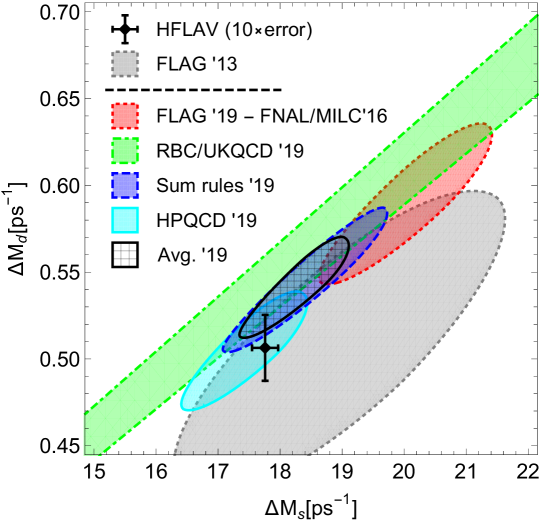
Figure 1: Predictions for ΔMsΔsubscript𝑀𝑠\Delta M_{s} and ΔMdΔsubscript𝑀𝑑\Delta M_{d}. See Section 2 for details.

To date several new determinations of the matrix elements with a precision below 10% have appeared: first from sum rules Grozin:2016uqy ; Grozin:2017uto ; Grozin:2018wtg ; Kirk:2017juj ; King:2019lal and very recently from the HPQCD collaboration Dowdall:2019bea . The SU(3) breaking ratios were also evaluated by the RBC/UKQCD collaboration Boyle:2018knm . We compare the various predictions in Fig. 1 where also the results using a weighted average of the values of Aoki:2019cca ; Kirk:2017juj ; King:2019lal ; Dowdall:2019bea ; Boyle:2018knm for the matrix elements are shown. The weighted average gives an impressive leap of the precision to 3.6% and 3.1% for the matrix elements for Bdsubscript𝐵𝑑B_{d} and Bssubscript𝐵𝑠B_{s} mixing. We observe excellent agreement between the sum rule prediction and the weighted average and given that lattice simulations and sum rules have very different systematic uncertainties this is a strong confirmation of both methods. We discuss the status of the non-perturbative input in more detail in Section 2. With respect to Eq. (1.5) and Eq. (1.6) the weighted averages

ΔMdAverage 2019Δsuperscriptsubscript𝑀𝑑Average 2019\displaystyle\Delta M_{d}^{\text{Average 2019}} =(0.5330.036+0.022)ps1=(1.050.07+0.04)ΔMdexp,absentsuperscriptsubscript0.5330.0360.022superscriptps1superscriptsubscript1.050.070.04Δsuperscriptsubscript𝑀𝑑exp\displaystyle=\left(0.533_{-0.036}^{+0.022}\right)\text{ps}^{-1}=\left(1.05_{-0.07}^{+0.04}\right)\Delta M_{d}^{\text{exp}}\,, (1.7)
ΔMsAverage 2019Δsuperscriptsubscript𝑀𝑠Average 2019\displaystyle\Delta M_{s}^{\text{Average 2019}} =(18.41.2+0.7)ps1=(1.040.07+0.04)ΔMsexp,absentsuperscriptsubscript18.41.20.7superscriptps1superscriptsubscript1.040.070.04Δsuperscriptsubscript𝑀𝑠exp\displaystyle=\left(18.4_{-1.2}^{+0.7}\right)\text{ps}^{-1}=\left(1.04_{-0.07}^{+0.04}\right)\Delta M_{s}^{\text{exp}}\,, (1.8)

show better agreement with experiment and a reduction of the total errors by about 40% to the point where the hadronic and parametric CKM uncertainties are of the same size.

We study the mass difference within the SM in more detail in Section 2 and give our estimate for the accuracy of the matrix elements in about five years time. Together with the extrapolation for the precision of the CKM elements presented in Kou:2018nap we expect

ΔMsFuture 2025Δsuperscriptsubscript𝑀𝑠Future 2025\displaystyle\Delta M_{s}^{\text{Future 2025}} =(18.4±0.5)ps1=(1.04±0.03)ΔMsexp.absentplus-or-minus18.40.5superscriptps1plus-or-minus1.040.03Δsuperscriptsubscript𝑀𝑠exp\displaystyle=\left(18.4\pm 0.5\right)\text{ps}^{-1}=\left(1.04\pm 0.03\right)\Delta M_{s}^{\text{exp}}\,. (1.9)

for a future (similar-to\sim 2025) scenario when the current bs𝑏𝑠b\to s\ell\ell anomalies should be established at the level of about 10 standard deviations if the central values remain the same Bediaga:2018lhg . In Section 3 we investigate the implications of Bssubscript𝐵𝑠B_{s} mixing on the bs𝑏𝑠b\to s\ell\ell anomalies in the FLAG ’19, Average ’19 and Future ’25 scenarios. First, we assume minimal Zsuperscript𝑍Z^{\prime} and lepto-quark (LQ) scenarios with only the couplings required to address the anomalies. Then, we discuss the viability of model-building ideas beyond the minimal Zsuperscript𝑍Z^{\prime} scenario that might reduce the theory value for ΔMsΔsubscript𝑀𝑠\Delta M_{s} and thus improve the agreement with experiment. Finally, we conclude in Section 4.

2 ΔMsΔsubscript𝑀𝑠\Delta M_{s} in the Standard Model

Refer to caption
Figure 2: Box diagrams that generate the Bs\mathit{{\mathit{{B}{}_{\mspace{-3.0mu}\scriptstyle{}}^{\mspace{-1.0mu}\scriptstyle{}}}}{}_{\mspace{-3.0mu}\scriptstyle{\mathit{{s}{}_{\mspace{-3.0mu}\scriptstyle{}}^{\mspace{-1.0mu}\scriptstyle{}}}}}^{\mspace{-1.0mu}\scriptstyle{}}}-B¯s\mathit{{\mkern 4.0mu\overline{\mkern-4.0mu{\mathit{{B}{}_{\mspace{-3.0mu}\scriptstyle{}}^{\mspace{-1.0mu}\scriptstyle{}}}}}}{}_{\mspace{-2.0mu}\scriptstyle{\mathit{{s}{}_{\mspace{-3.0mu}\scriptstyle{}}^{\mspace{-1.0mu}\scriptstyle{}}}}}^{\mspace{0.0mu}\scriptstyle{}}} mixing process in the SM. M12ssuperscriptsubscript𝑀12𝑠M_{12}^{s} is generated when the internal particles are off-shell.

In the SM, Bs\mathit{{\mathit{{B}{}_{\mspace{-3.0mu}\scriptstyle{}}^{\mspace{-1.0mu}\scriptstyle{}}}}{}_{\mspace{-3.0mu}\scriptstyle{\mathit{{s}{}_{\mspace{-3.0mu}\scriptstyle{}}^{\mspace{-1.0mu}\scriptstyle{}}}}}^{\mspace{-1.0mu}\scriptstyle{}}} mixing is generated by the diagrams shown in Fig. 2. The observable of interest in this work is the mass difference of the two mass eigenstates:

ΔMsMHsMLs=2|M12s|.Δsubscript𝑀𝑠subscriptsuperscript𝑀𝑠𝐻subscriptsuperscript𝑀𝑠𝐿2superscriptsubscript𝑀12𝑠\Delta M_{s}\equiv M^{s}_{H}-M^{s}_{L}=2\left|M_{12}^{s}\right|\,. (2.1)

The SM calculation (see e.g. Artuso:2015swg for a review) gives the following result for M12ssuperscriptsubscript𝑀12𝑠M_{12}^{s}

M12s,SM=GF212π2λt2MW2S0(xt)η^BfBs2MBsB1,M_{12}^{s,\,\text{SM}}=\frac{G_{F}^{2}}{12\pi^{2}}\lambda_{t}^{2}M_{W}^{2}S_{0}(x_{t})\hat{\eta}_{B}f_{\mathit{{\mathit{{B}{}_{\mspace{-3.0mu}\scriptstyle{}}^{\mspace{-1.0mu}\scriptstyle{}}}}{}_{\mspace{-3.0mu}\scriptstyle{\mathit{{s}{}_{\mspace{-3.0mu}\scriptstyle{}}^{\mspace{-1.0mu}\scriptstyle{}}}}}^{\mspace{-1.0mu}\scriptstyle{}}}}^{2}M_{\mathit{{\mathit{{B}{}_{\mspace{-3.0mu}\scriptstyle{}}^{\mspace{-1.0mu}\scriptstyle{}}}}{}_{\mspace{-3.0mu}\scriptstyle{\mathit{{s}{}_{\mspace{-3.0mu}\scriptstyle{}}^{\mspace{-1.0mu}\scriptstyle{}}}}}^{\mspace{-1.0mu}\scriptstyle{}}}}B_{1}\,, (2.2)

where λt=VtbVtssubscript𝜆𝑡subscript𝑉𝑡𝑏subscript𝑉𝑡𝑠\lambda_{t}=V_{tb}V_{*}{ts}, S0subscript𝑆0S_{0} is the Inami-Lim function Inami:1980fz , xt=(m¯t(m¯t)/MW)2subscript𝑥𝑡superscriptsubscript¯𝑚𝑡subscript¯𝑚𝑡subscript𝑀𝑊2x_{t}=\left(\bar{m}_{t}(\bar{m}_{t})/M_{W}\right)^{2} and η^B0.84subscript^𝜂𝐵0.84\hat{\eta}_{B}\approx 0.84 encodes the 2-loop perturbative QCD corrections Buras:1990fn . In the SM, only a single four-quark ΔB=2Δ𝐵2\Delta B=2 operator arises,

Q1=s¯γμ(1γ5)bs¯γμ(1γ5)b,Q_{1}=\mathit{{\mkern 4.0mu\overline{\mkern-4.0mu{s}}}{}_{\mspace{-2.0mu}\scriptstyle{}}^{\mspace{0.0mu}\scriptstyle{}}}\gamma^{\mu}(1-\gamma^{5})\mathit{{b}{}_{\mspace{-3.0mu}\scriptstyle{}}^{\mspace{-1.0mu}\scriptstyle{}}}\,\,\mathit{{\mkern 4.0mu\overline{\mkern-4.0mu{s}}}{}_{\mspace{-2.0mu}\scriptstyle{}}^{\mspace{0.0mu}\scriptstyle{}}}\gamma_{\mu}(1-\gamma^{5})\mathit{{b}{}_{\mspace{-3.0mu}\scriptstyle{}}^{\mspace{-1.0mu}\scriptstyle{}}}\,, (2.3)

whose hadronic matrix element is parameterised in terms of the meson decay constant fBsf_{\mathit{{\mathit{{B}{}_{\mspace{-3.0mu}\scriptstyle{}}^{\mspace{-1.0mu}\scriptstyle{}}}}{}_{\mspace{-3.0mu}\scriptstyle{\mathit{{s}{}_{\mspace{-3.0mu}\scriptstyle{}}^{\mspace{-1.0mu}\scriptstyle{}}}}}^{\mspace{-1.0mu}\scriptstyle{}}}} and a bag parameter B1subscript𝐵1B_{1}

Q1=Bs|Q1|B¯s83MBs2fBs2B1(μb).\braket{Q_{1}}=\braket{\mathit{{\mathit{{B}{}_{\mspace{-3.0mu}\scriptstyle{}}^{\mspace{-1.0mu}\scriptstyle{}}}}{}_{\mspace{-3.0mu}\scriptstyle{\mathit{{s}{}_{\mspace{-3.0mu}\scriptstyle{}}^{\mspace{-1.0mu}\scriptstyle{}}}}}^{\mspace{-1.0mu}\scriptstyle{}}}}{Q_{1}}{\mathit{{\mkern 4.0mu\overline{\mkern-4.0mu{\mathit{{B}{}_{\mspace{-3.0mu}\scriptstyle{}}^{\mspace{-1.0mu}\scriptstyle{}}}}}}{}_{\mspace{-2.0mu}\scriptstyle{\mathit{{s}{}_{\mspace{-3.0mu}\scriptstyle{}}^{\mspace{-1.0mu}\scriptstyle{}}}}}^{\mspace{0.0mu}\scriptstyle{}}}}\equiv\frac{8}{3}M_{\mathit{{\mathit{{B}{}_{\mspace{-3.0mu}\scriptstyle{}}^{\mspace{-1.0mu}\scriptstyle{}}}}{}_{\mspace{-3.0mu}\scriptstyle{\mathit{{s}{}_{\mspace{-3.0mu}\scriptstyle{}}^{\mspace{-1.0mu}\scriptstyle{}}}}}^{\mspace{-1.0mu}\scriptstyle{}}}}^{2}f_{\mathit{{\mathit{{B}{}_{\mspace{-3.0mu}\scriptstyle{}}^{\mspace{-1.0mu}\scriptstyle{}}}}{}_{\mspace{-3.0mu}\scriptstyle{\mathit{{s}{}_{\mspace{-3.0mu}\scriptstyle{}}^{\mspace{-1.0mu}\scriptstyle{}}}}}^{\mspace{-1.0mu}\scriptstyle{}}}}^{2}B_{1}(\mu_{b})\,. (2.4)

Note that we have used a form of Eq. 2.2 (matching that in Artuso:2015swg ) where the bag parameter B1subscript𝐵1B_{1} depends on the b\mathit{{b}{}_{\mspace{-3.0mu}\scriptstyle{}}^{\mspace{-1.0mu}\scriptstyle{}}} quark scale μbmbsimilar-tosubscript𝜇𝑏subscript𝑚𝑏\mu_{b}\sim m_{b}. An alternative notation (commonly used by lattice groups, for example see FLAG Aoki:2019cca ) uses the pair (ηB,B^1)subscript𝜂𝐵subscript^𝐵1(\eta_{B},\hat{B}_{1}) instead of (η^B,B1(μb))subscript^𝜂𝐵subscript𝐵1subscript𝜇𝑏(\hat{\eta}_{B},B_{1}(\mu_{b})), with B^1subscript^𝐵1\hat{B}_{1} a renormalization group (RG) invariant quantity. The two are related such that their product is equal, and explicitly we have

B^1=αs(μb)6/23(1+αs(μb)4π51653174)B1(μb)=1.519B1(μb).subscript^𝐵1subscript𝛼𝑠superscriptsubscript𝜇𝑏6231subscript𝛼𝑠subscript𝜇𝑏4𝜋51653174subscript𝐵1subscript𝜇𝑏1.519subscript𝐵1subscript𝜇𝑏\hat{B}_{1}=\alpha_{s}(\mu_{b})^{-6/23}\left(1+\frac{\alpha_{s}(\mu_{b})}{4\pi}\frac{5165}{3174}\right)B_{1}(\mu_{b})=1.519\,B_{1}(\mu_{b})\,. (2.5)

The combination fBs2B1f_{\mathit{{\mathit{{B}{}_{\mspace{-3.0mu}\scriptstyle{}}^{\mspace{-1.0mu}\scriptstyle{}}}}{}_{\mspace{-3.0mu}\scriptstyle{\mathit{{s}{}_{\mspace{-3.0mu}\scriptstyle{}}^{\mspace{-1.0mu}\scriptstyle{}}}}}^{\mspace{-1.0mu}\scriptstyle{}}}}^{2}B_{1} is the least-well known parameter for Bs\mathit{{\mathit{{B}{}_{\mspace{-3.0mu}\scriptstyle{}}^{\mspace{-1.0mu}\scriptstyle{}}}}{}_{\mspace{-3.0mu}\scriptstyle{\mathit{{s}{}_{\mspace{-3.0mu}\scriptstyle{}}^{\mspace{-1.0mu}\scriptstyle{}}}}}^{\mspace{-1.0mu}\scriptstyle{}}} mixing, and the most important as the observable ΔMsΔsubscript𝑀𝑠\Delta M_{s} is directly proportional to it. In the SM determination of the decay rate difference ΔΓqΔsubscriptΓ𝑞\Delta\Gamma_{q} and for BSM contributions to ΔMqΔsubscript𝑀𝑞\Delta M_{q} in addition to Q1subscript𝑄1Q_{1} four more operators arise:

Q2subscript𝑄2\displaystyle Q_{2} =s¯i(1γ5)bis¯j(1γ5)bj,Q3=s¯i(1γ5)bjs¯j(1γ5)bi,formulae-sequenceabsentsubscript¯𝑠𝑖1superscript𝛾5subscript𝑏𝑖subscript¯𝑠𝑗1superscript𝛾5subscript𝑏𝑗subscript𝑄3subscript¯𝑠𝑖1superscript𝛾5subscript𝑏𝑗subscript¯𝑠𝑗1superscript𝛾5subscript𝑏𝑖\displaystyle=\bar{s}_{i}(1-\gamma^{5})b_{i}\,\,\bar{s}_{j}(1-\gamma^{5})b_{j}\,,\hskip 28.45274ptQ_{3}=\bar{s}_{i}(1-\gamma^{5})b_{j}\,\,\bar{s}_{j}(1-\gamma^{5})b_{i}\,,
Q4subscript𝑄4\displaystyle Q_{4} =s¯i(1γ5)bis¯j(1+γ5)bj,Q5=s¯i(1γ5)bjs¯j(1+γ5)bi,formulae-sequenceabsentsubscript¯𝑠𝑖1superscript𝛾5subscript𝑏𝑖subscript¯𝑠𝑗1superscript𝛾5subscript𝑏𝑗subscript𝑄5subscript¯𝑠𝑖1superscript𝛾5subscript𝑏𝑗subscript¯𝑠𝑗1superscript𝛾5subscript𝑏𝑖\displaystyle=\bar{s}_{i}(1-\gamma^{5})b_{i}\,\,\bar{s}_{j}(1+\gamma^{5})b_{j}\,,\hskip 28.45274ptQ_{5}=\bar{s}_{i}(1-\gamma^{5})b_{j}\,\,\bar{s}_{j}(1+\gamma^{5})b_{i}\,, (2.6)

which are typically parameterised as

Q2delimited-⟨⟩subscript𝑄2\displaystyle\langle Q_{2}\rangle =fBs2MBs25MBs23(m¯b(μb)+m¯s(μb))2B2(μb),absentsuperscriptsubscript𝑓subscript𝐵𝑠2superscriptsubscript𝑀subscript𝐵𝑠25superscriptsubscript𝑀subscript𝐵𝑠23superscriptsubscript¯𝑚𝑏subscript𝜇𝑏subscript¯𝑚𝑠subscript𝜇𝑏2subscript𝐵2subscript𝜇𝑏\displaystyle=f_{B_{s}}^{2}M_{B_{s}}^{2}\,\frac{-5M_{B_{s}}^{2}}{3(\bar{m}_{b}(\mu_{b})+\bar{m}_{s}(\mu_{b}))^{2}}\,B_{2}(\mu_{b})\,,
Q3delimited-⟨⟩subscript𝑄3\displaystyle\langle Q_{3}\rangle =fBs2MBs2MBs23(m¯b(μb)+m¯s(μb))2B3(μb),absentsuperscriptsubscript𝑓subscript𝐵𝑠2superscriptsubscript𝑀subscript𝐵𝑠2superscriptsubscript𝑀subscript𝐵𝑠23superscriptsubscript¯𝑚𝑏subscript𝜇𝑏subscript¯𝑚𝑠subscript𝜇𝑏2subscript𝐵3subscript𝜇𝑏\displaystyle=f_{B_{s}}^{2}M_{B_{s}}^{2}\,\frac{M_{B_{s}}^{2}}{3(\bar{m}_{b}(\mu_{b})+\bar{m}_{s}(\mu_{b}))^{2}}\,B_{3}(\mu_{b})\,,
Q4delimited-⟨⟩subscript𝑄4\displaystyle\langle Q_{4}\rangle =fBs2MBs2[2MBs2(m¯b(μb)+m¯s(μb))2+13]B4(μb),absentsuperscriptsubscript𝑓subscript𝐵𝑠2superscriptsubscript𝑀subscript𝐵𝑠2delimited-[]2superscriptsubscript𝑀subscript𝐵𝑠2superscriptsubscript¯𝑚𝑏subscript𝜇𝑏subscript¯𝑚𝑠subscript𝜇𝑏213subscript𝐵4subscript𝜇𝑏\displaystyle=f_{B_{s}}^{2}M_{B_{s}}^{2}\,\left[\frac{2M_{B_{s}}^{2}}{(\bar{m}_{b}(\mu_{b})+\bar{m}_{s}(\mu_{b}))^{2}}+\frac{1}{3}\right]\,B_{4}(\mu_{b})\,,
Q5delimited-⟨⟩subscript𝑄5\displaystyle\langle Q_{5}\rangle =fBs2MBs2[2MBs23(m¯b(μb)+m¯s(μb))2+1]B5(μb).absentsuperscriptsubscript𝑓subscript𝐵𝑠2superscriptsubscript𝑀subscript𝐵𝑠2delimited-[]2superscriptsubscript𝑀subscript𝐵𝑠23superscriptsubscript¯𝑚𝑏subscript𝜇𝑏subscript¯𝑚𝑠subscript𝜇𝑏21subscript𝐵5subscript𝜇𝑏\displaystyle=f_{B_{s}}^{2}M_{B_{s}}^{2}\,\left[\frac{2M_{B_{s}}^{2}}{3(\bar{m}_{b}(\mu_{b})+\bar{m}_{s}(\mu_{b}))^{2}}+1\right]\,B_{5}(\mu_{b})\,. (2.7)

The full basis of matrix elements has been determined with lattice simulations Carrasco:2013zta ; Bazavov:2016nty ; Dowdall:2019bea and sum rules Kirk:2017juj ; King:2019lal . In Bazavov:2016nty the combinations fBs2Bisuperscriptsubscript𝑓subscript𝐵𝑠2subscript𝐵𝑖f_{B_{s}}^{2}B_{i} were determined and combined with the 2016 PDG average for the decay constants to extract the Bag parameters. This implies that the latter suffer from bigger uncertainties because one cannot exploit partial cancellations of uncertainties which occur when fBssubscript𝑓subscript𝐵𝑠f_{B_{s}} is determined in the same simulation. All other works determine the Bag parameters Bi(μb)subscript𝐵𝑖subscript𝜇𝑏B_{i}(\mu_{b}) as their central results. This has the advantage that the values can easily be combined with updated results for the decay constant fBssubscript𝑓subscript𝐵𝑠f_{B_{s}} which has seen significant improvements in the last few years and we use the FLAG 2++1++1 average Aoki:2019cca of the results Bussone:2016iua ; Hughes:2017spc ; Bazavov:2017lyh below.

In fact the sum rule method directly determines the Bag parameters and requires an independent result for the decay constant to obtain the matrix elements. In this approach one has to determine the perturbative 3-loop contribution to a correlator describing B𝐵B mixing. Based on the master integrals presented in Grozin:2008nu this calculation was first performed for Bdsubscript𝐵𝑑B_{d} mixing by Grozin:2016uqy ; Grozin:2017uto ; Grozin:2018wtg and confirmed in Kirk:2017juj , where this method was also extended to different mixing operators and to lifetime operators. In King:2019lal corrections due to a finite value of the strange quark mass were determined, yielding new predictions for the mass differences in better agreement with experiment than the FNAL/MILC values (Eqs. 1.5 and 1.6) with similar precision.
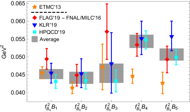
Refer to caption
Figure 3: Comparison of non-perturbative determinations of the matrix elements for Bssubscript𝐵𝑠B_{s} mixing at the scale μb=m¯b(m¯b)subscript𝜇𝑏subscript¯𝑚𝑏subscript¯𝑚𝑏\mu_{b}=\bar{m}_{b}(\bar{m}_{b}). We show the ETMC ’13 values in orange, the FLAG 2+1 average Aoki:2019cca for the operator Q1subscript𝑄1Q_{1} together with the FNAL/MILC ’16 results Bazavov:2016nty for the other operators in red, the sum rule values King:2019lal in blue and the HPQCD ’19 results Dowdall:2019bea in cyan. The gray rectangles indicate the weighted averages of the first three determinations.

Very recently an independent lattice study was performed by HPQCD Dowdall:2019bea which does not confirm the large FNAL/MILC predictions for the mass differences. We present a comparison of the combinations fBs2Bisuperscriptsubscript𝑓subscript𝐵𝑠2subscript𝐵𝑖f_{B_{s}}^{2}B_{i} in Fig. 3. Besides the individual results Carrasco:2013zta ; Aoki:2019cca ; Bazavov:2016nty ; King:2019lal ; Dowdall:2019bea we show the weighted averages thereof where we have excluded Carrasco:2013zta which only uses two dynamical flavours. For fBs2B1superscriptsubscript𝑓subscript𝐵𝑠2subscript𝐵1f_{B_{s}}^{2}B_{1}, which determines the SM value of the mass difference, the FLAG ’19 and HPQCD ’19 values do not overlap. However, the overall average shows perfect agreement with the KLR ’19 and ETMC ’13 results despite the very different systematic uncertainties of lattice simulation and sum rules. This makes us confident that the weighted average represents a reliable assessment of the current uncertainties. The different values of fBs2B2superscriptsubscript𝑓subscript𝐵𝑠2subscript𝐵2f_{B_{s}}^{2}B_{2} agree well. The case of fBs2B3superscriptsubscript𝑓subscript𝐵𝑠2subscript𝐵3f_{B_{s}}^{2}B_{3} is similar to that of the SM matrix element but the uncertainties are considerably larger. Finally for fBs2B4superscriptsubscript𝑓subscript𝐵𝑠2subscript𝐵4f_{B_{s}}^{2}B_{4} and fBs2B5superscriptsubscript𝑓subscript𝐵𝑠2subscript𝐵5f_{B_{s}}^{2}B_{5} we find a discrepancy between the results from ETMC ’13 and the remaining ones. This difference might result from the use of RI-MOM renormalisation scheme in Carrasco:2013zta , see e.g. the discussion in Garron:2016mva for a similar problem in the K𝐾K sector. The other values are in good agreement with each other, with KLR ’19 yielding a somewhat larger result than the lattice simulations for fBs2B5superscriptsubscript𝑓subscript𝐵𝑠2subscript𝐵5f_{B_{s}}^{2}B_{5}. Our weighted averages at the scale μb=m¯b(m¯b)subscript𝜇𝑏subscript¯𝑚𝑏subscript¯𝑚𝑏\mu_{b}=\bar{m}_{b}(\bar{m}_{b}) read

fBs2B1(μb)superscriptsubscript𝑓subscript𝐵𝑠2subscript𝐵1subscript𝜇𝑏\displaystyle f_{B_{s}}^{2}B_{1}(\mu_{b}) =(0.0452±0.0014)GeV2,absentplus-or-minus0.04520.0014superscriptGeV2\displaystyle=(0.0452\pm 0.0014)\,\text{GeV}^{2}\,,
fBs2B2(μb)superscriptsubscript𝑓subscript𝐵𝑠2subscript𝐵2subscript𝜇𝑏\displaystyle f_{B_{s}}^{2}B_{2}(\mu_{b}) =(0.0441±0.0017)GeV2,absentplus-or-minus0.04410.0017superscriptGeV2\displaystyle=(0.0441\pm 0.0017)\,\text{GeV}^{2}\,,
fBs2B3(μb)superscriptsubscript𝑓subscript𝐵𝑠2subscript𝐵3subscript𝜇𝑏\displaystyle f_{B_{s}}^{2}B_{3}(\mu_{b}) =(0.0454±0.0027)GeV2,absentplus-or-minus0.04540.0027superscriptGeV2\displaystyle=(0.0454\pm 0.0027)\,\text{GeV}^{2}\,,
fBs2B4(μb)superscriptsubscript𝑓subscript𝐵𝑠2subscript𝐵4subscript𝜇𝑏\displaystyle f_{B_{s}}^{2}B_{4}(\mu_{b}) =(0.0544±0.0019)GeV2,absentplus-or-minus0.05440.0019superscriptGeV2\displaystyle=(0.0544\pm 0.0019)\,\text{GeV}^{2}\,,
fBs2B5(μb)superscriptsubscript𝑓subscript𝐵𝑠2subscript𝐵5subscript𝜇𝑏\displaystyle f_{B_{s}}^{2}B_{5}(\mu_{b}) =(0.0507±0.0017)GeV2.absentplus-or-minus0.05070.0017superscriptGeV2\displaystyle=(0.0507\pm 0.0017)\,\text{GeV}^{2}\,. (2.8)

For convenience we also provide the weighted averages for Bdsubscript𝐵𝑑B_{d} mixing and the Bag parameters in A.

Refer to caption
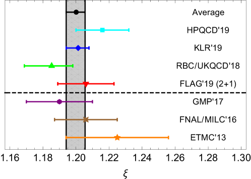
Figure 4: Comparison of determinations of the SU(3)-flavour breaking ratio ξ𝜉\xi. The gray band corresponds to the weighted average of the results Aoki:2019cca ; Boyle:2018knm ; King:2019lal ; Dowdall:2019bea . Below the dashed line we also show the values from Carrasco:2013zta ; Bazavov:2016nty ; Grozin:2017uto which are not included in the average.

The ratio of the mass differences of Bssubscript𝐵𝑠B_{s} and Bdsubscript𝐵𝑑B_{d} mesons benefits from the cancellation of many uncertainties and in the SM we get

ΔMdΔMs=|Vtd2Vts2|MBdMBsfB2B1BdfBs2B1Bs|Vtd2Vts2|MBdMBsξ2.Δsubscript𝑀𝑑Δsubscript𝑀𝑠superscriptsubscript𝑉𝑡𝑑2superscriptsubscript𝑉𝑡𝑠2subscript𝑀subscript𝐵𝑑subscript𝑀subscript𝐵𝑠superscriptsubscript𝑓𝐵2superscriptsubscript𝐵1subscript𝐵𝑑superscriptsubscript𝑓subscript𝐵𝑠2superscriptsubscript𝐵1subscript𝐵𝑠superscriptsubscript𝑉𝑡𝑑2superscriptsubscript𝑉𝑡𝑠2subscript𝑀subscript𝐵𝑑subscript𝑀subscript𝐵𝑠superscript𝜉2\frac{\Delta M_{d}}{\Delta M_{s}}=\left|\frac{V_{td}^{2}}{V_{ts}^{2}}\right|\frac{M_{B_{d}}}{M_{B_{s}}}\frac{f_{B}^{2}B_{1}^{B_{d}}}{f_{B_{s}}^{2}B_{1}^{B_{s}}}\equiv\left|\frac{V_{td}^{2}}{V_{ts}^{2}}\right|\frac{M_{B_{d}}}{M_{B_{s}}}\xi^{-2}\,. (2.9)

Different determinations Carrasco:2013zta ; Bazavov:2016nty ; Grozin:2017uto ; Boyle:2018knm ; Aoki:2019cca ; King:2019lal ; Dowdall:2019bea of the ratio ξ𝜉\xi are compared in Fig. 4 and we observe good agreement. The weighted average

ξ=1.2000.0060+0.0054𝜉superscriptsubscript1.2000.00600.0054\xi=1.200_{-0.0060}^{+0.0054} (2.10)

of the values from Boyle:2018knm ; Aoki:2019cca ; King:2019lal ; Dowdall:2019bea is dominated by the sum rule result King:2019lal which is about a factor of two more precise than the lattice determinations. Using the CKMFitter result

|Vtd/Vts|=0.20880.0030+0.0016,subscript𝑉𝑡𝑑subscript𝑉𝑡𝑠superscriptsubscript0.20880.00300.0016|V_{td}/V_{ts}|=0.2088_{-0.0030}^{+0.0016}\,, (2.11)

the ratio of the mass differences becomes

(ΔMdΔMs)expsubscriptΔsubscript𝑀𝑑Δsubscript𝑀𝑠exp\displaystyle\left(\frac{\Delta M_{d}}{\Delta M_{s}}\right)_{\text{exp}} =0.0285±0.0001,absentplus-or-minus0.02850.0001\displaystyle=0.0285\pm 0.0001\,, (2.12)
(ΔMdΔMs)AveragesubscriptΔsubscript𝑀𝑑Δsubscript𝑀𝑠Average\displaystyle\left(\frac{\Delta M_{d}}{\Delta M_{s}}\right)_{\text{Average}} =0.02980.0009+0.0005=0.02970.0003+0.0003(had.)0.0008+0.0005(CKM),absentsuperscriptsubscript0.02980.00090.0005superscriptsubscript0.02970.00030.0003superscriptsubscripthad.0.00080.0005CKM\displaystyle=0.0298_{-0.0009}^{+0.0005}=0.0297_{-0.0003}^{+0.0003}\,(\text{had.})_{-0.0008}^{+0.0005}\,(\text{CKM})\,, (2.13)

where the parametric CKM uncertainty (2.11) dominates theory error. We note that there is a slightly discrepancy between our average and experiment, at the level of 1.4 σsimilar-toabsenttimes1.4𝜎\sim$1.4\text{\,}\sigma$. This allows a very precise determination of |Vtd/Vts|subscript𝑉𝑡𝑑subscript𝑉𝑡𝑠|V_{td}/V_{ts}| from B𝐵B mixing King:2019lal . We note that the product of (2.13) and (1.8) is about 3% larger than the value for ΔMdΔsubscript𝑀𝑑\Delta M_{d} from a direct determination (1.7). The reason is that we also include the RBC/UKQCD ’18 Boyle:2018knm result in the average (2.10) for ξ𝜉\xi but not in the averages for the individual matrix elements since those were not determined there.222Furthermore the mean of a ratio is not the same as the ratio of the means. The ellipses in Fig. 1 use fBs2B1superscriptsubscript𝑓subscript𝐵𝑠2subscript𝐵1f_{B_{s}}^{2}B_{1} and ξ𝜉\xi as inputs and the ellipse for the weighted average therefore also gives a value of ΔMdΔsubscript𝑀𝑑\Delta M_{d} which is about 3% larger than (1.7). We further note that our ellipses for the FLAG ’19 and HPQCD ’19 results differ from the numerical results given in Bazavov:2016nty and Dowdall:2019bea because we use different values for the CKM parameters as discussed in A.

All in all we observe a consistent picture of different non-perturbative determinations for B𝐵B mixing. The future (similar-to\sim 2025) prospects for lattice simulations of the matrix elements have been assessed in Kou:2018nap ; Cerri:2018ypt . The relative uncertainties for fBs2B1superscriptsubscript𝑓subscript𝐵𝑠2subscript𝐵1f_{B_{s}}^{2}B_{1} are estimated as 3% Kou:2018nap and 1.3% Cerri:2018ypt . Given that the two latest lattice results Bazavov:2016nty ; Dowdall:2019bea do not overlap within their uncertainties and differ by 15% we believe the latter estimate to be overly optimistic and assume the scenario of Kou:2018nap . On the other hand the uncertainties in sum rule analyses are dominated by the one from the matching between QCD and Heavy Quark Effective Theory (HQET) matrix elements which can be reduced significantly by a perturbative two-loop matching calculation Grozin:2017uto ; Grozin:2018wtg or eliminated altogether by using QCD Korner:2003zk ; Mannel:2007am instead of HQET sum rules. We expect that a reduction of the sum rule uncertainty for B1subscript𝐵1B_{1} to 3% is realistic. The effect on the weighted average is a reduction of the error from 3.1% to about 2%.

Simultaneously, new experimental data from Belle II and the LHC will improve our knowledge of the CKM element Vcbsubscript𝑉𝑐𝑏V_{cb} which constrains Vtssubscript𝑉𝑡𝑠V_{ts} in the CKM unitarity fits and is the other critical input to our theory predictions. The Belle II collaboration forecasts Kou:2018nap that by 2025 the uncertainty on Vcbsubscript𝑉𝑐𝑏V_{cb} will be at the level of 1%. Using these future predictions (our explicit future inputs are given in Table 1, with all others staying the same as at present), we expect that ΔMsΔsubscript𝑀𝑠\Delta M_{s} will be predicted with an uncertainty of only ±0.5 \ps1times\pm0.5invps\pm 0.5\text{\,}\mathrm{\ps^{-1}} by 2025, yielding Eq. 1.9.333 It is worth noting that with such a precision, the FLAG 2019 central value given in Eq. 1.6 is almost 5 σtimes5𝜎5\text{\,}\sigma away from the experimental result.

Parameter Future value
Vcbsubscript𝑉𝑐𝑏V_{cb} 0.04240±1%=0.04240±0.00042plus-or-minus0.04240percent1plus-or-minus0.042400.000420.04240\pm 1\%=0.04240\pm 0.00042
fBsB^1f_{\mathit{{\mathit{{B}{}_{\mspace{-3.0mu}\scriptstyle{}}^{\mspace{-1.0mu}\scriptstyle{}}}}{}_{\mspace{-3.0mu}\scriptstyle{\mathit{{s}{}_{\mspace{-3.0mu}\scriptstyle{}}^{\mspace{-1.0mu}\scriptstyle{}}}}}^{\mspace{-1.0mu}\scriptstyle{}}}}\sqrt{\hat{B}_{1}} (262±1%) MeV=262±2.6 MeVtimesplus-or-minus262percent1megaelectronvolttimesuncertain2622.6megaelectronvolt$(262\pm 1\%)\text{\,}\mathrm{MeV}$=$262\pm 2.6\text{\,}\mathrm{MeV}$
Table 1: Future values for the two most important parameters for the error on ΔMsΔsubscript𝑀𝑠\Delta M_{s}.

3 ΔMsΔsubscript𝑀𝑠\Delta M_{s} interplay with flavour anomalies

3.1 Status and future prospects of the bs𝑏𝑠b\to s\ell\ell anomalies

A key application of the refined SM prediction for ΔMsΔsubscript𝑀𝑠\Delta M_{s} is in the context of the recent hints of lepton flavour universality (LFU) violation in semi-leptonic B\mathit{{B}{}_{\mspace{-3.0mu}\scriptstyle{}}^{\mspace{-1.0mu}\scriptstyle{}}} meson decays. Focussing on neutral current anomalies, the main observables are the LFU violating ratios RK()(BK()μ+μ)/(BK()e+e)subscript𝑅superscript𝐾𝐵superscript𝐾superscript𝜇superscript𝜇𝐵superscript𝐾superscript𝑒superscript𝑒R_{K^{(*)}}\equiv\mathcal{B}(B\to K^{(*)}\mu^{+}\mu^{-})/\mathcal{B}(B\to K^{(*)}e^{+}e^{-}) Aaij:2014ora ; Aaij:2017vbb ; Aaij:2019wad , together with the angular distributions of BK()μ+μ𝐵superscript𝐾superscript𝜇superscript𝜇B\to K^{(*)}\mu^{+}\mu^{-} Aaij:2015esa ; Khachatryan:2015isa ; Lees:2015ymt ; Wei:2009zv ; Aaltonen:2011ja ; Aaij:2015oid ; Abdesselam:2016llu ; Wehle:2016yoi ; Sirunyan:2017dhj ; Aaboud:2018krd and the branching ratios of hadronic bsμ+μ𝑏𝑠superscript𝜇superscript𝜇b\to s\mu^{+}\mu^{-} decays Aaij:2014pli ; Aaij:2015esa ; Khachatryan:2015isa . The effective Lagrangian for semi-leptonic bsμ+μ𝑏𝑠superscript𝜇superscript𝜇b\to s\mu^{+}\mu^{-} transitions contains the terms

bsμμNP4GF2VtbVts(δC9μO9μ+δC10μO10μ+δC9μO9μ+δC10μO10μ)+h.c.,4subscript𝐺𝐹2subscript𝑉𝑡𝑏subscript𝑉𝑡𝑠𝛿subscriptsuperscript𝐶𝜇9subscriptsuperscript𝑂𝜇9𝛿subscriptsuperscript𝐶𝜇10subscriptsuperscript𝑂𝜇10𝛿subscriptsuperscript𝐶𝜇9subscriptsuperscript𝑂𝜇9𝛿subscriptsuperscript𝐶𝜇10subscriptsuperscript𝑂𝜇10h.c.subscriptsuperscriptNP𝑏𝑠𝜇𝜇\mathcal{L}^{\text{NP}}_{b\to s\mu\mu}\supset\frac{4G_{F}}{\sqrt{2}}V_{tb}V_{*}{ts}\left(\delta C^{\mu}_{9}O^{\mu}_{9}+\delta C^{\mu}_{10}O^{\mu}_{10}+\delta C^{\prime\mu}_{9}O^{\prime\mu}_{9}+\delta C^{\prime\mu}_{10}O^{\prime\mu}_{10}\right)+\text{h.c.}\,, (3.1)

with

O9μsubscriptsuperscript𝑂𝜇9\displaystyle O^{\mu}_{9} =α4π(s¯LγμbL)(μ¯γμμ),\displaystyle=\frac{\alpha}{4\pi}(\mathit{{\mkern 4.0mu\overline{\mkern-4.0mu{s}}}{}_{\mspace{-2.0mu}\scriptstyle{}}^{\mspace{0.0mu}\scriptstyle{}}}_{L}\gamma_{\mu}\mathit{{b}{}_{\mspace{-3.0mu}\scriptstyle{}}^{\mspace{-1.0mu}\scriptstyle{}}}_{L})(\bar{\mu}\gamma^{\mu}\mu)\,, (3.2)
O10μsubscriptsuperscript𝑂𝜇10\displaystyle O^{\mu}_{10} =α4π(s¯LγμbL)(μ¯γμγ5μ),\displaystyle=\frac{\alpha}{4\pi}(\mathit{{\mkern 4.0mu\overline{\mkern-4.0mu{s}}}{}_{\mspace{-2.0mu}\scriptstyle{}}^{\mspace{0.0mu}\scriptstyle{}}}_{L}\gamma_{\mu}\mathit{{b}{}_{\mspace{-3.0mu}\scriptstyle{}}^{\mspace{-1.0mu}\scriptstyle{}}}_{L})(\bar{\mu}\gamma^{\mu}\gamma_{5}\mu)\,, (3.3)

and the primed operators O9,10μsubscriptsuperscript𝑂𝜇910O^{\prime\mu}_{9,10} having the opposite (LR𝐿𝑅L\to R) quark chiralities. Intriguingly, one obtains a very good description of the bs𝑏𝑠b\to s\ell\ell data by allowing new physics only in a single combination of Wilson coefficients (for recent fits see e.g. Aebischer:2019mlg ; Alguero:2019ptt ; Kowalska:2019ley ; Ciuchini:2019usw ; Arnan:2019uhr ; DAmico:2017mtc ; Alok:2019ufo ). The best-fit scenario δC9μ=δC10μ0.53±0.08𝛿superscriptsubscript𝐶9𝜇𝛿superscriptsubscript𝐶10𝜇plus-or-minus0.530.08\delta C_{9}^{\mu}=-\delta C_{10}^{\mu}\approx-0.53\pm 0.08 of Aebischer:2019mlg corresponds to an effective operator with left-handed (LH) quark and muon currents and we consider its interplay with ΔMsΔsubscript𝑀𝑠\Delta M_{s} in Section 3.4. The data is also well represented by assuming either δC9μ𝛿superscriptsubscript𝐶9𝜇\delta C_{9}^{\mu} or δC10μ𝛿superscriptsubscript𝐶10𝜇\delta C_{10}^{\mu} being different from zero, corresponding to vector or axial-vector muon currents, respectively. However, we find that the mixing constraints on these scenarios are stronger than for case of LH muon currents, since larger values of the Wilson coefficients are required, and do not discuss them further. Following the update of RKsubscript𝑅𝐾R_{K} from LHCb Aaij:2019wad , there has been an increased favourability of right handed (RH) current contributions in the quark sector and we investigate their effect in Section 3.5.2.

By 2025 LHCb expects a serious improvement in the measured precision on RKsubscript𝑅𝐾R_{K} and RKsubscript𝑅superscript𝐾R_{K^{*}} compared to the situation today – they forecast Bediaga:2018lhg the error on RKsubscript𝑅𝐾R_{K} will be reduced to ±0.025plus-or-minus0.025\pm 0.025 (better than a factor of two compared to the error reported at Moriond 2019) and to ±0.031plus-or-minus0.031\pm 0.031 for RKsubscript𝑅superscript𝐾R_{K^{*}} (a factor of four better). If these precisions are indeed realised, and the central values stay close to their currently measured values, LHCb will have made a discovery of LFU violation at the level of 6 σtimes6𝜎6\text{\,}\sigma and 10 σtimes10𝜎10\text{\,}\sigma for RKsubscript𝑅𝐾R_{K} and RK()subscript𝑅superscript𝐾R_{K^{(*)}} respectively.

3.2 New physics contributions to ΔMsΔsubscript𝑀𝑠\Delta M_{s} in the effective theory

The NP contributions to Bssubscript𝐵𝑠B_{s} mixing can be described by the effective Lagrangian

ΔB=2NPsubscriptsuperscriptNPΔ𝐵2\displaystyle\mathcal{L}^{\text{NP}}_{\Delta B=2} 4GF2(VtbVts)2[CbsLL(s¯LγμbL)2+CbsRR(s¯RγμbR)2\displaystyle\supset-\frac{4G_{F}}{\sqrt{2}}\left(V_{tb}V_{*}{ts}\right)^{2}\Big{[}C^{LL}_{bs}\left(\mathit{{\mkern 4.0mu\overline{\mkern-4.0mu{s}}}{}_{\mspace{-2.0mu}\scriptstyle{}}^{\mspace{0.0mu}\scriptstyle{}}}_{L}\gamma_{\mu}\mathit{{b}{}_{\mspace{-3.0mu}\scriptstyle{}}^{\mspace{-1.0mu}\scriptstyle{}}}_{L}\right)^{2}+C^{RR}_{bs}\left(\mathit{{\mkern 4.0mu\overline{\mkern-4.0mu{s}}}{}_{\mspace{-2.0mu}\scriptstyle{}}^{\mspace{0.0mu}\scriptstyle{}}}_{R}\gamma_{\mu}\mathit{{b}{}_{\mspace{-3.0mu}\scriptstyle{}}^{\mspace{-1.0mu}\scriptstyle{}}}_{R}\right)^{2}
+CbsLR(s¯LγμbL)(s¯RγμbR)]+h.c.,\displaystyle+C^{LR}_{bs}\left(\mathit{{\mkern 4.0mu\overline{\mkern-4.0mu{s}}}{}_{\mspace{-2.0mu}\scriptstyle{}}^{\mspace{0.0mu}\scriptstyle{}}}_{L}\gamma_{\mu}\mathit{{b}{}_{\mspace{-3.0mu}\scriptstyle{}}^{\mspace{-1.0mu}\scriptstyle{}}}_{L}\right)\left(\mathit{{\mkern 4.0mu\overline{\mkern-4.0mu{s}}}{}_{\mspace{-2.0mu}\scriptstyle{}}^{\mspace{0.0mu}\scriptstyle{}}}_{R}\gamma^{\mu}\mathit{{b}{}_{\mspace{-3.0mu}\scriptstyle{}}^{\mspace{-1.0mu}\scriptstyle{}}}_{R}\right)\Big{]}+\text{h.c.}\,, (3.4)

where we assume NP only gives rise to vector colour singlet operators. The full basis of ΔB=2Δ𝐵2\Delta B=2 operators (Eqs. 2.3 and 2.6) also contains operators that give tensor or scalar Dirac structures when written in colour singlet form. However, these operator structures are highly disfavoured by the fits to bs𝑏𝑠b\to s\ell\ell data, and so we ignore them here. Assuming the NP coefficients Cbssubscript𝐶𝑏𝑠C_{bs} are generated at some higher scale μNPsubscript𝜇NP\mu_{\text{NP}}, we have to include RG running effects down to the b\mathit{{b}{}_{\mspace{-3.0mu}\scriptstyle{}}^{\mspace{-1.0mu}\scriptstyle{}}} quark scale (see e.g. Bagger:1997gg ), which brings in the LR vector operator with the non colour singlet structure through operator mixing and explains the appearance of both B4subscript𝐵4B_{4} and B5subscript𝐵5B_{5} in the expression below. In this way we can parameterise the SM+NP contribution normalized to the SM one as444This expression neglects the top-quark threshold, which is a sub-percent effect. However, the correct running is taken into account in our numerics and figures.

ΔMsSM+NPΔMsSM=|1\displaystyle\frac{\Delta M_{s}^{\text{SM+NP}}}{\Delta M_{s}^{\text{SM}}}=\Bigg{|}1 +η6/23RloopSM{CbsLL+CbsRRCbsLR2η3/23[B5B1(MBs2(mb+ms)2+32)\displaystyle+\frac{\eta^{6/23}}{R_{\text{loop}}^{\text{SM}}}\Bigg{\{}C^{LL}_{bs}+C^{RR}_{bs}-\frac{C^{LR}_{bs}}{2\eta^{3/23}}\Bigg{[}\frac{B_{5}}{B_{1}}\left(\frac{M_{\mathit{{\mathit{{B}{}_{\mspace{-3.0mu}\scriptstyle{}}^{\mspace{-1.0mu}\scriptstyle{}}}}{}_{\mspace{-3.0mu}\scriptstyle{\mathit{{s}{}_{\mspace{-3.0mu}\scriptstyle{}}^{\mspace{-1.0mu}\scriptstyle{}}}}}^{\mspace{-1.0mu}\scriptstyle{}}}}^{2}}{(m_{b}+m_{s})^{2}}+\frac{3}{2}\right)
+B4B1(MBs2(mb+ms)2+16)(η27/231)]}|,\displaystyle+\frac{B_{4}}{B_{1}}\left(\frac{M_{\mathit{{\mathit{{B}{}_{\mspace{-3.0mu}\scriptstyle{}}^{\mspace{-1.0mu}\scriptstyle{}}}}{}_{\mspace{-3.0mu}\scriptstyle{\mathit{{s}{}_{\mspace{-3.0mu}\scriptstyle{}}^{\mspace{-1.0mu}\scriptstyle{}}}}}^{\mspace{-1.0mu}\scriptstyle{}}}}^{2}}{(m_{b}+m_{s})^{2}}+\frac{1}{6}\right)\left(\eta^{-27/23}-1\right)\Bigg{]}\Bigg{\}}\Bigg{|}\,, (3.5)

with η=αs(μNP)/αs(mb)𝜂subscript𝛼𝑠subscript𝜇NPsubscript𝛼𝑠subscript𝑚𝑏\eta=\alpha_{s}(\mu_{\text{NP}})/\alpha_{s}(m_{b}), the bag parameters Bisubscript𝐵𝑖B_{i} defined as in Eqs. 2.4 and 2.7, and the SM loop function given by

RSMloop=2GFMW2η^BS0(xt)16π2=(1.310±0.010)×103.subscriptsuperscript𝑅loopSM2subscript𝐺𝐹superscriptsubscript𝑀𝑊2subscript^𝜂𝐵subscript𝑆0subscript𝑥𝑡16superscript𝜋2plus-or-minus1.3100.010superscript103R^{\text{loop}}_{\text{SM}}=\frac{\sqrt{2}G_{F}M_{W}^{2}\hat{\eta}_{B}S_{0}(x_{t})}{16\pi^{2}}=(1.310\pm 0.010)\times 10^{-3}\,. (3.6)

In general, one would expect that any NP contributing to bs𝑏𝑠b\to s\ell\ell transitions will eventually feed into Bssubscript𝐵𝑠B_{s} mixing. However, this connection is hidden at the effective operator level where the Wilson coefficients in Eq. (3.1) and Eq. (3.2) are independent.555The double insertion of the effective Lagrangian for bs𝑏𝑠b\to s\ell\ell transitions (3.1) yields a contribution to ΔMsΔsubscript𝑀𝑠\Delta M_{s} at the dimension-eight level. Compared to the contribution from Eq. (3.2) this is suppressed by mb2/ΛNP2superscriptsubscript𝑚𝑏2superscriptsubscriptΛNP2m_{b}^{2}/\Lambda_{\text{NP}}^{2} and cannot be used to obtain meaningful constraints. It is hence crucial to focus on specific UV realizations in order to explore the connection between bs𝑏𝑠b\to s\ell\ell anomalies and ΔMsΔsubscript𝑀𝑠\Delta M_{s} and we will consider two simplified models below.

3.3 Simplified models for the bs𝑏𝑠b\to s\ell\ell anomalies

There are two basic possibilities how the effective operators in Eq. (3.1) can be generated at tree level: by the exchange of a Zsuperscript𝑍Z^{\prime} mediator coupling to the quark and the muon current or by the exchange of a lepto-quark coupling to mixed quark-muon currents. Anticipating our results from Section 3.4 we describe the Zsuperscript𝑍Z^{\prime} scenario in detail below. In addition we consider the case of the scalar lepto-quark S3(3,3,1/3)similar-tosubscript𝑆33313S_{3}\sim(3,3,1/3), whose defining Lagrangian can be found e.g. in DiLuzio:2017fdq ; Dorsner:2016wpm .

We consider a simplified Zsuperscript𝑍Z^{\prime} model with only those couplings required to explain the observed flavour anomalies, with the Lagrangian

Z12MZ2(Zμ)2+Zμ(λijQd¯LiγμdLi+λijdd¯RiγμdRj+λijL¯LiγμLj),\mathcal{L}_{Z^{\prime}}\supset\frac{1}{2}M_{Z^{\prime}}^{2}(Z^{\prime}_{\mu})^{2}+Z^{\prime}_{\mu}\left(\lambda^{Q}_{ij}\mathit{{\mkern 4.0mu\overline{\mkern-4.0mu{d}}}{}_{\mspace{-2.0mu}\scriptstyle{}}^{\mspace{0.0mu}\scriptstyle{}}}_{L}^{i}\gamma^{\mu}\mathit{{d}{}_{\mspace{-3.0mu}\scriptstyle{}}^{\mspace{-1.0mu}\scriptstyle{}}}_{L}^{i}+\lambda^{d}_{ij}\mathit{{\mkern 4.0mu\overline{\mkern-4.0mu{d}}}{}_{\mspace{-2.0mu}\scriptstyle{}}^{\mspace{0.0mu}\scriptstyle{}}}_{R}^{i}\gamma^{\mu}\mathit{{d}{}_{\mspace{-3.0mu}\scriptstyle{}}^{\mspace{-1.0mu}\scriptstyle{}}}_{R}^{j}+\lambda^{L}_{ij}\mathit{{\mkern 4.0mu\overline{\mkern-4.0mu{\ell}}}{}_{\mspace{-2.0mu}\scriptstyle{}}^{\mspace{0.0mu}\scriptstyle{}}}_{L}^{i}\gamma^{\mu}\mathit{{\ell}{}_{\mspace{-3.0mu}\scriptstyle{}}^{\mspace{-1.0mu}\scriptstyle{}}}_{L}^{j}\right)\,, (3.7)

where di\mathit{{d}{}_{\mspace{-3.0mu}\scriptstyle{}}^{\mspace{-1.0mu}\scriptstyle{}}}^{i} and i\mathit{{\ell}{}_{\mspace{-3.0mu}\scriptstyle{}}^{\mspace{-1.0mu}\scriptstyle{}}}^{i} label the different generations of down-type quark and charged lepton mass eigenstates respectively, and λQ,d,Lsuperscript𝜆𝑄𝑑𝐿\lambda^{Q,d,L} are hermitian flavour space matrices. We have neglected RH currents in the lepton sector in the above Eq. (3.7) since the latter actually worsen the compatibility with ΔMsΔsubscript𝑀𝑠\Delta M_{s}, as they require a larger Wilson coefficient.

Integrating out the Zsuperscript𝑍Z^{\prime} at tree level, we get the effective Lagrangian

Zeff12MZ2(\displaystyle\mathcal{L}^{\text{eff}}_{Z^{\prime}}\supset-\frac{1}{2M_{Z^{\prime}}^{2}}\bigg{(} 2λ23Qλ22L(s¯LγμbL)(μ¯LγμμL)+2λ23dλ22L(s¯RγμbR)(μ¯LγμμL)\displaystyle 2\lambda^{Q}_{23}\lambda^{L}_{22}(\mathit{{\mkern 4.0mu\overline{\mkern-4.0mu{s}}}{}_{\mspace{-2.0mu}\scriptstyle{}}^{\mspace{0.0mu}\scriptstyle{}}}_{L}\gamma^{\mu}\mathit{{b}{}_{\mspace{-3.0mu}\scriptstyle{}}^{\mspace{-1.0mu}\scriptstyle{}}}_{L})(\bar{\mu}_{L}\gamma_{\mu}\mu_{L})+2\lambda^{d}_{23}\lambda^{L}_{22}(\mathit{{\mkern 4.0mu\overline{\mkern-4.0mu{s}}}{}_{\mspace{-2.0mu}\scriptstyle{}}^{\mspace{0.0mu}\scriptstyle{}}}_{R}\gamma^{\mu}\mathit{{b}{}_{\mspace{-3.0mu}\scriptstyle{}}^{\mspace{-1.0mu}\scriptstyle{}}}_{R})(\bar{\mu}_{L}\gamma_{\mu}\mu_{L})
+(λ23Q)2(s¯LγμbL)(s¯LγμbL)\displaystyle+\left(\lambda^{Q}_{23}\right)^{2}(\mathit{{\mkern 4.0mu\overline{\mkern-4.0mu{s}}}{}_{\mspace{-2.0mu}\scriptstyle{}}^{\mspace{0.0mu}\scriptstyle{}}}_{L}\gamma^{\mu}\mathit{{b}{}_{\mspace{-3.0mu}\scriptstyle{}}^{\mspace{-1.0mu}\scriptstyle{}}}_{L})(\mathit{{\mkern 4.0mu\overline{\mkern-4.0mu{s}}}{}_{\mspace{-2.0mu}\scriptstyle{}}^{\mspace{0.0mu}\scriptstyle{}}}_{L}\gamma_{\mu}\mathit{{b}{}_{\mspace{-3.0mu}\scriptstyle{}}^{\mspace{-1.0mu}\scriptstyle{}}}_{L}) (3.8)
+(λ23d)2(s¯RγμbR)(s¯RγμbR)+2λ23Qλ23d(s¯LγμbL)(s¯RγμbR)).\displaystyle+\left(\lambda^{d}_{23}\right)^{2}(\mathit{{\mkern 4.0mu\overline{\mkern-4.0mu{s}}}{}_{\mspace{-2.0mu}\scriptstyle{}}^{\mspace{0.0mu}\scriptstyle{}}}_{R}\gamma^{\mu}\mathit{{b}{}_{\mspace{-3.0mu}\scriptstyle{}}^{\mspace{-1.0mu}\scriptstyle{}}}_{R})(\mathit{{\mkern 4.0mu\overline{\mkern-4.0mu{s}}}{}_{\mspace{-2.0mu}\scriptstyle{}}^{\mspace{0.0mu}\scriptstyle{}}}_{R}\gamma_{\mu}\mathit{{b}{}_{\mspace{-3.0mu}\scriptstyle{}}^{\mspace{-1.0mu}\scriptstyle{}}}_{R})+2\lambda^{Q}_{23}\lambda^{d}_{23}(\mathit{{\mkern 4.0mu\overline{\mkern-4.0mu{s}}}{}_{\mspace{-2.0mu}\scriptstyle{}}^{\mspace{0.0mu}\scriptstyle{}}}_{L}\gamma^{\mu}\mathit{{b}{}_{\mspace{-3.0mu}\scriptstyle{}}^{\mspace{-1.0mu}\scriptstyle{}}}_{L})(\mathit{{\mkern 4.0mu\overline{\mkern-4.0mu{s}}}{}_{\mspace{-2.0mu}\scriptstyle{}}^{\mspace{0.0mu}\scriptstyle{}}}_{R}\gamma_{\mu}\mathit{{b}{}_{\mspace{-3.0mu}\scriptstyle{}}^{\mspace{-1.0mu}\scriptstyle{}}}_{R})\bigg{)}\,.

The first line contains the terms that contribute to the rare decay coefficients C9,10()μsuperscriptsubscript𝐶910𝜇C_{9,10}^{(\prime)\mu}, the second a contribution to ΔMsΔsubscript𝑀𝑠\Delta M_{s} through the same operator as in the SM, and the third contributions to ΔMsΔsubscript𝑀𝑠\Delta M_{s} from operators that do not appear in the SM.

Matching onto the effective Lagrangians for the low energy observables in Eqs. 3.1 and 3.2, we find (at the scale μ=MZ𝜇subscript𝑀superscript𝑍\mu=M_{Z^{\prime}})

δC9μ=δC10μ𝛿superscriptsubscript𝐶9𝜇𝛿superscriptsubscript𝐶10𝜇\displaystyle\delta C_{9}^{\mu}=-\delta C_{10}^{\mu} =π2GFMZ2α(λ23Qλ22LVtbVts),absent𝜋2subscript𝐺𝐹subscriptsuperscript𝑀2superscript𝑍𝛼subscriptsuperscript𝜆𝑄23subscriptsuperscript𝜆𝐿22subscript𝑉𝑡𝑏subscript𝑉𝑡𝑠\displaystyle=-\frac{\pi}{\sqrt{2}G_{F}M^{2}_{Z^{\prime}}\alpha}\left(\frac{\lambda^{Q}_{23}\lambda^{L}_{22}}{V_{tb}V_{*}{ts}}\right)\,, (3.9)
δC9μ=δC10μ𝛿superscriptsubscript𝐶9𝜇𝛿superscriptsubscript𝐶10𝜇\displaystyle\delta C_{9}^{\prime\mu}=-\delta C_{10}^{\prime\mu} =π2GFMZ2α(λ23dλ22LVtbVts),absent𝜋2subscript𝐺𝐹subscriptsuperscript𝑀2superscript𝑍𝛼subscriptsuperscript𝜆𝑑23subscriptsuperscript𝜆𝐿22subscript𝑉𝑡𝑏subscript𝑉𝑡𝑠\displaystyle=-\frac{\pi}{\sqrt{2}G_{F}M^{2}_{Z^{\prime}}\alpha}\left(\frac{\lambda^{d}_{23}\lambda^{L}_{22}}{V_{tb}V_{*}{ts}}\right)\,, (3.10)
CbsLLsuperscriptsubscript𝐶𝑏𝑠𝐿𝐿\displaystyle C_{bs}^{LL} =142GFMZ2(λ23QVtbVts)2,absent142subscript𝐺𝐹subscriptsuperscript𝑀2superscript𝑍superscriptsubscriptsuperscript𝜆𝑄23subscript𝑉𝑡𝑏subscript𝑉𝑡𝑠2\displaystyle=\frac{1}{4\sqrt{2}G_{F}M^{2}_{Z^{\prime}}}\left(\frac{\lambda^{Q}_{23}}{V_{tb}V_{*}{ts}}\right)^{2}\,, (3.11)
CbsRRsuperscriptsubscript𝐶𝑏𝑠𝑅𝑅\displaystyle C_{bs}^{RR} =142GFMZ2(λ23dVtbVts)2,absent142subscript𝐺𝐹subscriptsuperscript𝑀2superscript𝑍superscriptsubscriptsuperscript𝜆𝑑23subscript𝑉𝑡𝑏subscript𝑉𝑡𝑠2\displaystyle=\frac{1}{4\sqrt{2}G_{F}M^{2}_{Z^{\prime}}}\left(\frac{\lambda^{d}_{23}}{V_{tb}V_{*}{ts}}\right)^{2}\,, (3.12)
CbsLRsuperscriptsubscript𝐶𝑏𝑠𝐿𝑅\displaystyle C_{bs}^{LR} =24GFMZ2(λ23Qλ23d(VtbVts)2).absent24subscript𝐺𝐹subscriptsuperscript𝑀2superscript𝑍subscriptsuperscript𝜆𝑄23subscriptsuperscript𝜆𝑑23superscriptsubscript𝑉𝑡𝑏subscript𝑉𝑡𝑠2\displaystyle=\frac{\sqrt{2}}{4G_{F}M^{2}_{Z^{\prime}}}\left(\frac{\lambda^{Q}_{23}\lambda^{d}_{23}}{(V_{tb}V_{*}{ts})^{2}}\right)\,. (3.13)

Inserting the above expressions in Section 3.2, using our combined averages for the bag parameters, and taking a typical Zsuperscript𝑍Z^{\prime} scale of 5 TeVtimes5teraelectronvolt5\text{\,}\mathrm{TeV} we find that the contribution to ΔMsΔsubscript𝑀𝑠\Delta M_{s} can be written as666The prefactor and the relative size of the interference term have a sub-leading logarithmic dependence from the Zsuperscript𝑍Z^{\prime} mass (less than 1% for MZsubscript𝑀superscript𝑍M_{Z^{\prime}} in the 110 TeVtimesrange110teraelectronvolt110\text{\,}\mathrm{TeV} range).

ΔMsSM+NPΔMsSM|1+200(5 TeVMZ)2[(λ23Q)2+(λ23d)29λ23Qλ23d]|,Δsuperscriptsubscript𝑀𝑠SM+NPΔsuperscriptsubscript𝑀𝑠SM1200superscripttimes5teraelectronvoltsubscript𝑀superscript𝑍2delimited-[]superscriptsubscriptsuperscript𝜆𝑄232superscriptsubscriptsuperscript𝜆𝑑2329subscriptsuperscript𝜆𝑄23subscriptsuperscript𝜆𝑑23\frac{\Delta M_{s}^{\text{SM+NP}}}{\Delta M_{s}^{\text{SM}}}\approx\left|1+200\left(\frac{$5\text{\,}\mathrm{TeV}$}{M_{Z^{\prime}}}\right)^{2}\left[\left(\lambda^{Q}_{23}\right)^{2}+\left(\lambda^{d}_{23}\right)^{2}-9\lambda^{Q}_{23}\lambda^{d}_{23}\right]\right|\,, (3.14)

which shows a significant RG enhancement for the LR operator.

Besides Bssubscript𝐵𝑠B_{s} mixing, we consider a constraint that is particularly relevant for light Zsuperscript𝑍Z^{\prime} interacting with muons via LH currents. By SU(2)L𝑆𝑈subscript2𝐿SU(2)_{L} invariance the Zsuperscript𝑍Z^{\prime} couples also to LH neutrinos via the λ22Lsubscriptsuperscript𝜆𝐿22\lambda^{L}_{22} coupling which is required by the bsμμ𝑏𝑠𝜇𝜇b\to s\mu\mu anomalies. Hence, one has an extra term in the Zsuperscript𝑍Z^{\prime} effective Lagrangian of the type

Zeff(λ22L)2MZ2(μ¯LγμμL)(ν¯μLγμνμL),superscriptsubscriptsuperscript𝜆𝐿222superscriptsubscript𝑀superscript𝑍2subscript¯𝜇𝐿superscript𝛾𝜇subscript𝜇𝐿subscript¯𝜈𝜇𝐿superscript𝛾𝜇subscript𝜈𝜇𝐿subscriptsuperscripteffsuperscript𝑍\mathcal{L}^{\text{eff}}_{Z^{\prime}}\supset-\frac{(\lambda^{L}_{22})^{2}}{M_{Z^{\prime}}^{2}}(\bar{\mu}_{L}\gamma^{\mu}\mu_{L})(\bar{\nu}_{\mu L}\gamma^{\mu}\nu_{\mu L})\,, (3.15)

which leads to the neutrino trident production, νμNνμμ+μNsubscript𝜈𝜇𝑁subscript𝜈𝜇superscript𝜇superscript𝜇𝑁\nu_{\mu}N\to\nu_{\mu}\mu^{+}\mu^{-}N. Using the most recent calculation for the SM cross-section, one gets Altmannshofer:2019zhy

σCCFRSM+NPσCCFRSM=1.13(1+v2(λ22L)2MZ2)2+(1+4sW2+v2(λ22L)2MZ2)21.13+(1+4sW2)2subscriptsuperscript𝜎SMNPCCFRsubscriptsuperscript𝜎SMCCFR1.13superscript1superscript𝑣2superscriptsubscriptsuperscript𝜆𝐿222subscriptsuperscript𝑀2superscript𝑍2superscript14subscriptsuperscript𝑠2𝑊superscript𝑣2superscriptsubscriptsuperscript𝜆𝐿222subscriptsuperscript𝑀2superscript𝑍21.13superscript14subscriptsuperscript𝑠2𝑊2\frac{\sigma^{\rm SM+NP}_{\rm CCFR}}{\sigma^{\rm SM}_{\rm CCFR}}=\frac{1.13\left(1+\frac{v^{2}(\lambda^{L}_{22})^{2}}{M^{2}_{Z^{\prime}}}\right)^{2}+\left(1+4s^{2}_{W}+\frac{v^{2}(\lambda^{L}_{22})^{2}}{M^{2}_{Z^{\prime}}}\right)^{2}}{1.13+(1+4s^{2}_{W})^{2}} (3.16)

(with v246𝑣246v\approx 246 GeV and sW20.231subscriptsuperscript𝑠2𝑊0.231s^{2}_{W}\approx 0.231), which is constrained by the existing CCFR measurement σCCFR/σCCFRSM=0.82±0.28subscript𝜎CCFRsubscriptsuperscript𝜎SMCCFRplus-or-minus0.820.28\sigma_{\rm CCFR}/\sigma^{\rm SM}_{\rm CCFR}=0.82\pm 0.28 Mishra:1991bv . This result implies MZ/λ22L>0.47 TeVsubscript𝑀superscript𝑍subscriptsuperscript𝜆𝐿22times0.47teraelectronvoltM_{Z^{\prime}}/\lambda^{L}_{22}>$0.47\text{\,}\mathrm{TeV}$ at 2 σtimes2𝜎2\text{\,}\sigma. The upcoming DUNE experiment Abi:2018dnh is expected to also measure this process, however the precision it will achieve (see e.g. Altmannshofer:2019zhy ), suggest its data will not increase much the limits on this parameter combination and so we will use the CCFR bound throughout.

Last but not least, the parameter space is constrained by direct LHC searches Aaboud:2017buh ; Sirunyan:2017yrk and perturbative unitarity DiLuzio:2017chi ; DiLuzio:2016sur . Whether a few TeV Zsuperscript𝑍Z^{\prime} is ruled out by LHC direct searches crucially depends on the details of the Zsuperscript𝑍Z^{\prime} model. The stringent constraints from di-lepton searches Aaboud:2017buh are tamed in models where the Zsuperscript𝑍Z^{\prime} does not couple to valence quarks. For instance, assuming only the two couplings required by the bs𝑏𝑠b\to s\ell\ell anomaly, namely λ23Qsubscriptsuperscript𝜆𝑄23\lambda^{Q}_{23} and λ22Lsubscriptsuperscript𝜆𝐿22\lambda^{L}_{22}, one finds that current Zsuperscript𝑍Z^{\prime} searches are not sensitive yet (see e.g. Allanach:2017bta ; Afik:2018nlr ). Assuming the best-fit scenario δC9μ=δC10μ0.53±0.08𝛿superscriptsubscript𝐶9𝜇𝛿superscriptsubscript𝐶10𝜇plus-or-minus0.530.08\delta C_{9}^{\mu}=-\delta C_{10}^{\mu}\approx-0.53\pm 0.08 Aebischer:2019mlg is generated by the exchange of a Zsuperscript𝑍Z^{\prime} we obtain the perturbative unitarity bound MZ<59 TeVsubscript𝑀superscript𝑍times59teraelectronvoltM_{Z^{\prime}}<$59\text{\,}\mathrm{TeV}$ DiLuzio:2017chi . The same limit for the lepto-quark scenario reads MS3<69 TeVsubscript𝑀subscript𝑆3times69teraelectronvoltM_{S_{3}}<$69\text{\,}\mathrm{TeV}$ DiLuzio:2017chi . The mass of the lepto-quark is also bounded from below up to about 1 TeVtimes1teraelectronvolt1\text{\,}\mathrm{TeV} Sirunyan:2017yrk from direct searches at the LHC.

3.4 ΔMsΔsubscript𝑀𝑠\Delta M_{s} interplay with flavour anomalies in the minimal scenarios

We investigate which new physics contributions ΔMsNPΔsuperscriptsubscript𝑀𝑠NP\Delta M_{s}^{\text{NP}} to the Bssubscript𝐵𝑠B_{s} mass difference are generated by the simplified models of Section 3.3, assuming LH currents in the quark sector and real couplings (these two assumptions will be relaxed in Section 3.5). We obtain the predictions

ΔMsSM+NPΔMsSMΔsuperscriptsubscript𝑀𝑠SM+NPΔsuperscriptsubscript𝑀𝑠SM\displaystyle\frac{\Delta M_{s}^{\text{SM+NP}}}{\Delta M_{s}^{\text{SM}}} =|1+GFαEM2η6/2322π2RloopSM(δC9μ=δC10μ)2(MZλ22L)2|absent1subscript𝐺𝐹superscriptsubscript𝛼EM2superscript𝜂62322superscript𝜋2superscriptsubscript𝑅loopSMsuperscript𝛿superscriptsubscript𝐶9𝜇𝛿superscriptsubscript𝐶10𝜇2superscriptsubscript𝑀superscript𝑍subscriptsuperscript𝜆𝐿222\displaystyle=\left|1+\frac{G_{F}\alpha_{\text{EM}}^{2}\eta^{6/23}}{2\sqrt{2}\pi^{2}R_{\text{loop}}^{\text{SM}}}\left(\delta C_{9}^{\mu}=-\delta C_{10}^{\mu}\right)^{2}\left(\frac{M_{Z^{\prime}}}{\lambda^{L}_{22}}\right)^{2}\right| (3.17)
|1+1360(δC9μ=δC10μ0.53)2(MZ/λ22L1 TeV)2|,absent11360superscript𝛿superscriptsubscript𝐶9𝜇𝛿superscriptsubscript𝐶10𝜇0.532superscriptsubscript𝑀superscript𝑍subscriptsuperscript𝜆𝐿22times1teraelectronvolt2\displaystyle\approx\left|1+\frac{1}{360}\left(\frac{\delta C_{9}^{\mu}=-\delta C_{10}^{\mu}}{-0.53}\right)^{2}\left(\frac{M_{Z^{\prime}}/\lambda^{L}_{22}}{$1\text{\,}\mathrm{TeV}$}\right)^{2}\right|\,,

for the Zsuperscript𝑍Z^{\prime} and

ΔMsSM+NPΔMsSMΔsuperscriptsubscript𝑀𝑠SM+NPΔsuperscriptsubscript𝑀𝑠SM\displaystyle\frac{\Delta M_{s}^{\text{SM+NP}}}{\Delta M_{s}^{\text{SM}}} =|1+GFαEM2η6/2322π2RloopSM564π2(δC9μ=δC10μ)2(MS3)2|absent1subscript𝐺𝐹superscriptsubscript𝛼EM2superscript𝜂62322superscript𝜋2superscriptsubscript𝑅loopSM564superscript𝜋2superscript𝛿superscriptsubscript𝐶9𝜇𝛿superscriptsubscript𝐶10𝜇2superscriptsubscript𝑀subscript𝑆32\displaystyle=\left|1+\frac{G_{F}\alpha_{\text{EM}}^{2}\eta^{6/23}}{2\sqrt{2}\pi^{2}R_{\text{loop}}^{\text{SM}}}\frac{5}{64\pi^{2}}\left(\delta C_{9}^{\mu}=-\delta C_{10}^{\mu}\right)^{2}\left(M_{S_{3}}\right)^{2}\right| (3.18)
|1+129 000(δC9μ=δC10μ0.53)2(MS31 TeV)2|,absent1129000superscript𝛿superscriptsubscript𝐶9𝜇𝛿superscriptsubscript𝐶10𝜇0.532superscriptsubscript𝑀subscript𝑆3times1teraelectronvolt2\displaystyle\approx\left|1+\frac{1}{$29\,000$}\left(\frac{\delta C_{9}^{\mu}=-\delta C_{10}^{\mu}}{-0.53}\right)^{2}\left(\frac{M_{S_{3}}}{$1\text{\,}\mathrm{TeV}$}\right)^{2}\right|\,,

for the lepto-quark.

Refer to caption
Refer to caption
Refer to caption
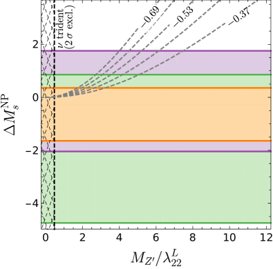
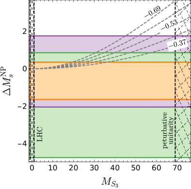
Figure 5: We show the predicted new physics effects ΔMsNPΔsuperscriptsubscript𝑀𝑠NP\Delta M_{s}^{\rm NP} (dashed lines) for various values of δC9μ=δC10μ𝛿superscriptsubscript𝐶9𝜇𝛿superscriptsubscript𝐶10𝜇\delta C_{9}^{\mu}=-\delta C_{10}^{\mu} in comparison with the allowed two-sigma regions (shaded) in the FLAG ’19, Avg. ’19 and Future ’25 scenarios. The left and right panel assume the simplified Zsuperscript𝑍Z^{\prime} model and scalar lepto-quark model, respectively. Hatched regions show limits from neutrino trident production or direct LHC searches and perturbative unitarity.

In Fig. 5 we compare the new physics contributions ΔMsNPΔsuperscriptsubscript𝑀𝑠NP\Delta M_{s}^{\text{NP}} in the two models to the allowed two-sigma regions for the present and future scenarios. The dashed lines show what effect is predicted for a given value of the Wilson coefficient combination δC9μ=δC10μ𝛿superscriptsubscript𝐶9𝜇𝛿superscriptsubscript𝐶10𝜇\delta C_{9}^{\mu}=-\delta C_{10}^{\mu}, whereby the envelope of these lines corresponds to the two-sigma region from the fit δC9μ=δC10μ=0.53±0.08𝛿superscriptsubscript𝐶9𝜇𝛿superscriptsubscript𝐶10𝜇plus-or-minus0.530.08\delta C_{9}^{\mu}=-\delta C_{10}^{\mu}=-0.53\pm 0.08 to the present bs𝑏𝑠b\to s\ell\ell data. In addition we show constraints from neutrino trident production, direct searches by the LHC experiments and perturbative unitarity as hatched regions.

The left plot shows the simplified Zsuperscript𝑍Z^{\prime} model where the relation between ΔMsΔsubscript𝑀𝑠\Delta M_{s} and δC9𝛿subscript𝐶9\delta C_{9} depends on the parameter combination MZ/λ22Lsubscript𝑀superscript𝑍subscriptsuperscript𝜆𝐿22M_{Z^{\prime}}/\lambda^{L}_{22}. We observe that a Zsuperscript𝑍Z^{\prime} explanation of the bs𝑏𝑠b\to s\ell\ell data causes a sizeable positive contribution to ΔMsΔsubscript𝑀𝑠\Delta M_{s} unless the Zsuperscript𝑍Z^{\prime} mass is rather light. Values of ΔMsNPΔsuperscriptsubscript𝑀𝑠NP\Delta M_{s}^{\text{NP}} outside the shaded regions are in tension with the respective predictions for ΔMsΔsubscript𝑀𝑠\Delta M_{s} at the level of two standard deviations. This allows us to place upper bounds on the mass of the Zsuperscript𝑍Z^{\prime}.777A full statistical fit would be in order here to make a definitive statement about some particular model being excluded. For instance, we find that the large central value of the FLAG ’19 prediction in Eq. (1.6) (green region) requires MZ4 TeVless-than-or-similar-tosuperscriptsubscript𝑀𝑍times4teraelectronvoltM_{Z}^{\prime}\lesssim$4\text{\,}\mathrm{TeV}$ for λ22L=1subscriptsuperscript𝜆𝐿221\lambda^{L}_{22}=1 in order to explain bs𝑏𝑠b\to s\ell\ell at 1 σtimes1𝜎1\text{\,}\sigma. The limit is about a factor 3/232\nicefrac{{3}}{{2}} weaker in the case of the Average ’19 value of ΔMsΔsubscript𝑀𝑠\Delta M_{s} (purple region) despite the reduction of the uncertainty by over 30% with respect to FLAG ’19 because the central value is closer to the experimental result. It is straightforward to rescale the bound for different lepton couplings. The combination of ΔMsΔsubscript𝑀𝑠\Delta M_{s} and perturbative unitarity (requiring λ22L<4πsubscriptsuperscript𝜆𝐿224𝜋\lambda^{L}_{22}<\sqrt{4\pi} DiLuzio:2017chi ; DiLuzio:2016sur ) gives an upper bound of MZ20 TeVless-than-or-similar-tosubscript𝑀superscript𝑍times20teraelectronvoltM_{Z^{\prime}}\lesssim$20\text{\,}\mathrm{TeV}$ from the Average ’19 prediction. With the future scenario for ΔMsΔsubscript𝑀𝑠\Delta M_{s} (orange region) this will improve to about 9 TeVtimes9teraelectronvolt9\text{\,}\mathrm{TeV}, being a factor of 6 more constraining than the perturbative unitarity bound DiLuzio:2017chi ; DiLuzio:2016sur .

The lepto-quark model is shown in the right plot and yields smaller new physics contributions to ΔMsΔsubscript𝑀𝑠\Delta M_{s} because the effect is only generated at loop level. Using the Average ’19 value (purple) we find that a lepto-quark explanation is still viable in the entire mass range between the LHC and unitarity constraints. However, the increased precision of the Future ’25 scenario implies an upper limit of about 30 TeVtimes30teraelectronvolt30\text{\,}\mathrm{TeV} on the lepto-quark mass MS3subscript𝑀subscript𝑆3M_{S_{3}}, better than the perturbativity bound by more than a factor of two.

We conclude that both simplified Zsuperscript𝑍Z^{\prime} and lepto-quark models currently provide possible solutions to the bs𝑏𝑠b\to s\ell\ell anomalies, with the previous stringent constraints DiLuzio:2017fdq from the FLAG ’19 values for ΔMsΔsubscript𝑀𝑠\Delta M_{s} being relaxed by the refined SM prediction Average ’19. However, with the future increase in the precision of ΔMsΔsubscript𝑀𝑠\Delta M_{s} lepto-quark explanations will be favoured over a Zsuperscript𝑍Z^{\prime}, assuming that the central values remain similar. In Section 3.5 we therefore discuss ideas how the implied tension might be reduced by generalizations of the minimal Zsuperscript𝑍Z^{\prime} scenario.

3.5 New physics options beyond the minimal Zsuperscript𝑍Z^{\prime} scenario

The constraints on the minimal Zsuperscript𝑍Z^{\prime} scenario considered above are particularly strong because the latter predicts a positive contribution to ΔMsΔsubscript𝑀𝑠\Delta M_{s}, while the central values of the current SM predictions are already larger than the experimental result. Therefore, we will explore two simple options for how a negative contribution to ΔMsΔsubscript𝑀𝑠\Delta M_{s} could be generated, thus relaxing the tension. Examining Eq. 3.14 the two cases present themselves:

  1. 1.

    For only LH quark coupling (i.e. λd=0superscript𝜆𝑑0\lambda^{d}=0), a negative contribution can only be generated if λ23Qsubscriptsuperscript𝜆𝑄23\lambda^{Q}_{23} acquires a complex phase.

  2. 2.

    With both LH and RH quark couplings, real couplings alone can give the required sign if the interference term is large enough.

Although these two possibilities were already identified in DiLuzio:2017fdq , their compatibility with global fits for flavour anomalies was only partially assessed in DiLuzio:2018wch . We start with CP violating couplings in Section 3.5.1, and then study the case for RH quark currents in Section 3.5.2. As a benchmark point, we take a lepton coupling of λ22L=1subscriptsuperscript𝜆𝐿221\lambda^{L}_{22}=1 and a Zsuperscript𝑍Z^{\prime} mass of 5 TeVtimes5teraelectronvolt5\text{\,}\mathrm{TeV} where the best-fit result δC9μ=δC10μ=0.53𝛿superscriptsubscript𝐶9𝜇𝛿superscriptsubscript𝐶10𝜇0.53\delta C_{9}^{\mu}=-\delta C_{10}^{\mu}=-0.53 saturates the two-sigma range of the Average ’19 prediction (see Fig. 5). In the following, we address the question whether either option 1. or 2. allows for this benchmark point to be viable within the FLAG ’19 or Future ’25 scenarios.

3.5.1 CP violating couplings

It is clear from Eq. 3.14 that if λ23Qsubscriptsuperscript𝜆𝑄23\lambda^{Q}_{23} has a large enough imaginary part, then it will be possible to bring down the theory prediction for ΔMsΔsubscript𝑀𝑠\Delta M_{s} below the SM prediction and into better agreement with experiment. However, once we allow for complex Zsuperscript𝑍Z^{\prime} quark couplings, there are extra constraints to be considered, in the form of CP-violating observables that arise from Bs\mathit{{\mathit{{B}{}_{\mspace{-3.0mu}\scriptstyle{}}^{\mspace{-1.0mu}\scriptstyle{}}}}{}_{\mspace{-3.0mu}\scriptstyle{\mathit{{s}{}_{\mspace{-3.0mu}\scriptstyle{}}^{\mspace{-1.0mu}\scriptstyle{}}}}}^{\mspace{-1.0mu}\scriptstyle{}}} mixing. The most relevant here is the mixing-induced CP asymmetry Lenz:2006hd ; Artuso:2015swg , arising from interference between B𝐵B meson mixing and decay. The semi-leptonic CP asymmetries for flavour-specific decays, aslssubscriptsuperscript𝑎𝑠sla^{s}_{\text{sl}}, are not competitive yet since the experimental errors are still too large Artuso:2015swg . Defining

ϕΔ=Arg(1+η6/23CbsLLRSMloop),subscriptitalic-ϕΔArg1superscript𝜂623subscriptsuperscript𝐶𝐿𝐿𝑏𝑠subscriptsuperscript𝑅loopSM\phi_{\Delta}=\text{Arg}\left(1+\frac{\eta^{6/23}C^{LL}_{bs}}{R^{\rm loop}_{\rm SM}}\right)\,, (3.19)

(with η𝜂\eta as in Section 3.2) the mixing-induced CP asymmetry is given by

ACPmix(BsJ/ψϕ)=sin(ϕΔ2βs),A^{\text{mix}}_{\text{CP}}(\mathit{{\mathit{{B}{}_{\mspace{-3.0mu}\scriptstyle{}}^{\mspace{-1.0mu}\scriptstyle{}}}}{}_{\mspace{-3.0mu}\scriptstyle{\mathit{{s}{}_{\mspace{-3.0mu}\scriptstyle{}}^{\mspace{-1.0mu}\scriptstyle{}}}}}^{\mspace{-1.0mu}\scriptstyle{}}}\to\mathit{{J\mspace{-2.0mu}/\mspace{-2.0mu}\psi}{}_{\mspace{-3.0mu}\scriptstyle{}}^{\mspace{-1.0mu}\scriptstyle{}}}\mathit{{\phi}{}_{\mspace{-3.0mu}\scriptstyle{}}^{\mspace{-1.0mu}\scriptstyle{}}})=\sin{\left(\phi_{\Delta}-2\beta_{s}\right)}\,, (3.20)

where ACPmix=0.021±0.031subscriptsuperscript𝐴mixCPplus-or-minus0.0210.031A^{\text{mix}}_{\text{CP}}=-0.021\pm 0.031 Amhis:2016xyh ; HFLAV:PDG2018 , βs=0.018430.00034+0.00048subscript𝛽𝑠subscriptsuperscript0.018430.000480.00034\beta_{s}=0.01843^{+0.00048}_{-0.00034} CKMfitter:Summer18 , and we have neglected penguin contributions Artuso:2015swg .

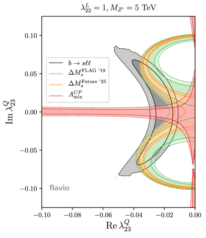
New phases in λ23Qsubscriptsuperscript𝜆𝑄23\lambda^{Q}_{23} also imply a complex value for δC9μ𝛿superscriptsubscript𝐶9𝜇\delta C_{9}^{\mu}, which has not typically been considered in previous global fits (see Alok:2017jgr ; Alda:2018mfy for exceptions). We perform our own fit using the flavio software Straub:2018kue , using the same set of bs𝑏𝑠b\to s\ell\ell observables as Altmannshofer:2017fio .

The result of our fit is shown in Fig. 6, with the higher SM prediction ΔMsFLAG ’19Δsuperscriptsubscript𝑀𝑠FLAG ’19\Delta M_{s}^{\text{FLAG '19}} corresponding to the green bands.

Refer to caption
Figure 6: Allowed regions at 1 σtimes1𝜎1\text{\,}\sigma (solid) and 2 σtimes2𝜎2\text{\,}\sigma (dashed) for bs𝑏𝑠b\to s\ell\ell (grey), ΔMsΔsubscript𝑀𝑠\Delta M_{s} (green (FLAG ’19) and orange (Future ’25)), and AmixCPsubscriptsuperscript𝐴CPmixA^{\text{CP}}_{\text{mix}} (red).

There is no overlap between the 1 σtimes1𝜎1\text{\,}\sigma regions for our three observables, since ACPmixsubscriptsuperscript𝐴mixCPA^{\text{mix}}_{\text{CP}} provides too strong a constraint on the imaginary part of the coupling. So a complex coupling does not provide a way to significantly evade the strong bounds from ΔMsΔsubscript𝑀𝑠\Delta M_{s}. Using instead our prediction ΔMsFuture ’25Δsuperscriptsubscript𝑀𝑠Future ’25\Delta M_{s}^{\text{Future '25}} (orange) there is still no overlap, for the same reason. As such, the addition of complex phases to the Zsuperscript𝑍Z^{\prime} quark coupling does not alleviate tension at the benchmark point in the Future ’25 scenario, which is important given the strength of this future bound, as shown in Fig. 5.

3.5.2 Right-handed couplings

A Zsuperscript𝑍Z^{\prime} coupling to a RH quark current can also allow for a negative BSM contribution to ΔMsΔsubscript𝑀𝑠\Delta M_{s} through the interference term, which has the advantage that it is RG enhanced by roughly an order of magnitude (see Eq. 3.14) relative to the pure LL or RR operators. In our previous work DiLuzio:2017fdq ; DiLuzio:2018wch we stated that RH quark currents break the approximate symmetry RKRKsubscript𝑅𝐾subscript𝑅superscript𝐾R_{K}\approx R_{K^{*}} and hence were disfavoured by the data. On the other hand, the recent update of RKsubscript𝑅𝐾R_{K} at Moriond 2019 Aaij:2019wad favours a non-zero RH quark current contribution, as widely discussed in the literature since then (see e.g. Aebischer:2019mlg ; Alguero:2019ptt ; Kowalska:2019ley ; Ciuchini:2019usw ; Arnan:2019uhr ; DAmico:2017mtc ; Alok:2019ufo ).

There is however a problem with this solution, which is that in our Zsuperscript𝑍Z^{\prime} model, at the leading order in the NP contribution, the behaviour can be written as

RK1RK1λ23Q+λ23dλ23Q(2p1)λ23d,subscript𝑅𝐾1subscript𝑅superscript𝐾1subscriptsuperscript𝜆𝑄23subscriptsuperscript𝜆𝑑23subscriptsuperscript𝜆𝑄232𝑝1subscriptsuperscript𝜆𝑑23\frac{R_{K}-1}{R_{K^{*}}-1}\approx\frac{\lambda^{Q}_{23}+\lambda^{d}_{23}}{\lambda^{Q}_{23}-(2p-1)\lambda^{d}_{23}}\,, (3.21)

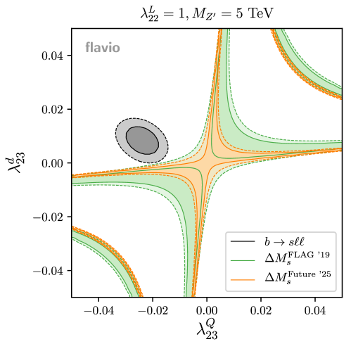
where p0.86𝑝0.86p\approx 0.86 is the polarization fraction Hiller:2014ula . The current experimental measurements suggest (RK1)/(RK1)0.50subscript𝑅𝐾1subscript𝑅superscript𝐾10.50(R_{K}-1)/(R_{K^{*}}-1)\approx 0.50, which requires λ23d/λ23Q0.37subscriptsuperscript𝜆𝑑23subscriptsuperscript𝜆𝑄230.37\lambda^{d}_{23}/\lambda^{Q}_{23}\approx-0.37. On the other hand, Eq. 3.14 shows that the same sign for LH and RH quark couplings are needed to reduce ΔMsΔsubscript𝑀𝑠\Delta M_{s}. This is evident in our fit result shown in Fig. 7, where the allowed region for the bs𝑏𝑠b\to s\ell\ell anomalies is partially driven by the RK()subscript𝑅superscript𝐾R_{K^{(*)}} measurements.

Refer to caption
Figure 7: Allowed regions at 1 σtimes1𝜎1\text{\,}\sigma (solid) and 2 σtimes2𝜎2\text{\,}\sigma (dashed) for bs𝑏𝑠b\to s\ell\ell (grey) and ΔMsΔsubscript𝑀𝑠\Delta M_{s} (green (FLAG ’19) and orange (Future ’25)).

With the high prediction ΔMsFLAG ’19Δsuperscriptsubscript𝑀𝑠FLAG ’19\Delta M_{s}^{\text{FLAG '19}}, there is a clear gap between the 1 σtimes1𝜎1\text{\,}\sigma allowed regions, which does not allow us to solve the tension for the benchmark point (for a similar conclusion see also Arnan:2019uhr ). If we instead examine the orange region, corresponding to the ΔMsFuture ’25Δsuperscriptsubscript𝑀𝑠Future ’25\Delta M_{s}^{\text{Future '25}} prediction,888For the numerics here we assume a similar relative improvement in the precision of the BSM bag parameters B4,5subscript𝐵45B_{4,5} as was described earlier for B1subscript𝐵1B_{1}. the gap has shrunk by only a small amount, and so our benchmark point is only marginally more favoured.

3.5.3 Beyond simplified Zsuperscript𝑍Z^{\prime} models

Within the simplified Zsuperscript𝑍Z^{\prime} model considered so far, neither of the two options above (imaginary couplings and RH quark currents) helps to improve the compatibility between the bs𝑏𝑠b\to s\ell\ell measurements and the expected precision determination value of ΔMsΔsubscript𝑀𝑠\Delta M_{s} in 2025. There are, however, other possibilities in order to achieve that when going beyond our simplified Zsuperscript𝑍Z^{\prime} setup. For instance, sticking only to RKsubscript𝑅𝐾R_{K} and RKsubscript𝑅superscript𝐾R_{K^{*}} (so no angular observables, etc.), these can be accommodated via NP in electrons featuring sizeable contributions both from LH and RH quark currents, so that a negative contribution to ΔMsΔsubscript𝑀𝑠\Delta M_{s} is possible as well. This class of models were suggested in the context of Composite Higgs scenarios Carmona:2017fsn . Alternatively, as pointed out in Bordone:2018nbg , in UV complete models of the vector lepto-quark Uμ(3,1,2/3)similar-tosubscript𝑈𝜇3123U_{\mu}\sim(3,1,2/3) DiLuzio:2017vat ; Calibbi:2017qbu ; Bordone:2017bld ; Barbieri:2017tuq ; Blanke:2018sro ; DiLuzio:2018zxy addressing both RD()subscript𝑅superscript𝐷R_{D^{(*)}} and bs𝑏𝑠b\to s\ell\ell anomalies, the couplings to quarks of extra Zsuperscript𝑍Z^{\prime} and/or coloron states (not directly responsible for the anomalies in semi-leptonic B𝐵B decays) can naturally have a large phase in order to accommodate a negative ΔMsΔsubscript𝑀𝑠\Delta M_{s}, without being in tension with CP violating observables. These two examples show that although it is difficult to obtain ΔMsNP<0Δsuperscriptsubscript𝑀𝑠NP0\Delta M_{s}^{\rm NP}<0 within simplified models for the bs𝑏𝑠b\to s\ell\ell anomalies, that is certainly not impossible in more general constructions.

4 Conclusions

In this paper, we have combined recent results from sum rules Kirk:2017juj ; King:2019lal (by some of the current authors, see also Grozin:2016uqy ; Grozin:2017uto ; Grozin:2018wtg for consistent results for the operator Q1subscript𝑄1Q_{1} by a different group), and the FNAL/MILC Bazavov:2016nty and HPQCD Dowdall:2019bea lattice collaborations into updated predictions for the mass differences

ΔMdAverage 2019Δsuperscriptsubscript𝑀𝑑Average 2019\displaystyle\Delta M_{d}^{\text{Average 2019}} =(0.5330.036+0.022)ps1=(1.050.07+0.04)ΔMdexp,absentsuperscriptsubscript0.5330.0360.022superscriptps1superscriptsubscript1.050.070.04Δsuperscriptsubscript𝑀𝑑exp\displaystyle=\left(0.533_{-0.036}^{+0.022}\right)\text{ps}^{-1}=\left(1.05_{-0.07}^{+0.04}\right)\Delta M_{d}^{\text{exp}}\,, (4.1)
ΔMsAverage 2019Δsuperscriptsubscript𝑀𝑠Average 2019\displaystyle\Delta M_{s}^{\text{Average 2019}} =(18.41.2+0.7)ps1=(1.040.07+0.04)ΔMsexp.absentsuperscriptsubscript18.41.20.7superscriptps1superscriptsubscript1.040.070.04Δsuperscriptsubscript𝑀𝑠exp\displaystyle=\left(18.4_{-1.2}^{+0.7}\right)\text{ps}^{-1}=\left(1.04_{-0.07}^{+0.04}\right)\Delta M_{s}^{\text{exp}}\,. (4.2)

These results are about 40% more precise than the values in Eq. (1.5) and Eq. (1.6) obtained from the current FLAG Aoki:2019cca averages and show better agreement with the experimental results. The average for the SU(3)-breaking ratio ξ𝜉\xi that determines the SM predictions for ΔMd/ΔMsΔsubscript𝑀𝑑Δsubscript𝑀𝑠\Delta M_{d}/\Delta M_{s} is dominated by the SR calculation combined with the most recent lattice results for the decay constants, which provides a precision much better than the lattice-alone value for this quantity. The new averages agree very well with the individual SR results (see Fig. 3 and Fig. 4), further reinforcing the usefulness of this as a totally independent determination of these important non-perturbative parameters. With our new average the hadronic uncertainties in these quantities are now at the same level as the CKM uncertainties. We then argued that with improved determinations of the hadronic matrix elements and the CKM elements the precision in ΔMsΔsubscript𝑀𝑠\Delta M_{s} can be improved to 3% by about 2025.

Refer to caption
Refer to caption
Refer to caption
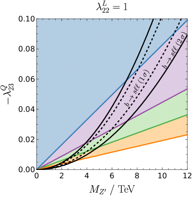
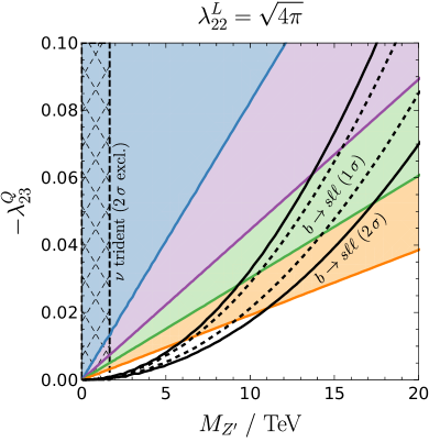
Figure 8: Parameter space of a naive Zsuperscript𝑍Z^{\prime} model explaining bs𝑏𝑠b\to s\ell\ell via real LH currents, for two representative lepton couplings: λ22L=1subscriptsuperscript𝜆𝐿221\lambda^{L}_{22}=1 (left panel) and λ22L=4πsubscriptsuperscript𝜆𝐿224𝜋\lambda^{L}_{22}=\sqrt{4\pi} (right panel). Constraints from various determinations of ΔMsΔsubscript𝑀𝑠\Delta M_{s} and neutrino trident production are shown as well.

We investigated the constraints from ΔMsΔsubscript𝑀𝑠\Delta M_{s} on minimal Zsuperscript𝑍Z^{\prime} and LQ explanations of the bs𝑏𝑠b\to s\ell\ell anomalies. The constraints for LQs are generally weaker because contributions to Bssubscript𝐵𝑠B_{s} mixing are only generated at loop level. Still we find that the assumed Future ’25 scenario leads to an upper bound of 30 TeVtimes30teraelectronvolt30\text{\,}\mathrm{TeV} on the LQ mass, stronger than the unitarity constraint DiLuzio:2017chi ; DiLuzio:2016sur by more than a factor of two. The situation for the Zsuperscript𝑍Z^{\prime} is summarized in Fig. 8. Despite the reduction of the uncertainty the constraints with the updated prediction Average ’19 are weaker by about a factor 3/232\nicefrac{{3}}{{2}} than those obtained with the FLAG ’19 scenario like in our earlier work DiLuzio:2017fdq because of the smaller central value. Nevertheless, Bssubscript𝐵𝑠B_{s} mixing by itself is sufficient to exclude the minimal Zsuperscript𝑍Z^{\prime} scenario with a benchmark value of λ22L=1subscriptsuperscript𝜆𝐿221\lambda^{L}_{22}=1 for the lepton coupling for Zsuperscript𝑍Z^{\prime} masses above 6 TeVtimes6teraelectronvolt6\text{\,}\mathrm{TeV}. Assuming the Future ’25 scenario, we obtain the upper limit MZ9 TeVless-than-or-similar-tosubscript𝑀superscript𝑍times9teraelectronvoltM_{Z^{\prime}}\lesssim$9\text{\,}\mathrm{TeV}$ for lepton couplings saturating the perturbativity bound (see right panel in Fig. 8), which is about six times better than the unitarity bound on the Zsuperscript𝑍Z^{\prime} mass. On the other hand, the left plot in Fig. 8 demonstrates that the parameter space will be very strongly constrained for more perturbative values of λ22Lsubscriptsuperscript𝜆𝐿22\lambda^{L}_{22}. An interesting open question is to what extent this mass window can be covered by direct searches at different future colliders.

Last but not least, we have addressed the question whether an extension of the minimal Zsuperscript𝑍Z^{\prime} scenario might relax the strong constraints. We have discussed two possibilities in which the minimal model might be extended, by adding new CP violating phases to the quark coupling, or including a coupling to both LH and RH quarks. For the case of new CP phases, the Bs\mathit{{\mathit{{B}{}_{\mspace{-3.0mu}\scriptstyle{}}^{\mspace{-1.0mu}\scriptstyle{}}}}{}_{\mspace{-3.0mu}\scriptstyle{\mathit{{s}{}_{\mspace{-3.0mu}\scriptstyle{}}^{\mspace{-1.0mu}\scriptstyle{}}}}}^{\mspace{-1.0mu}\scriptstyle{}}} mixing observable AmixCPsubscriptsuperscript𝐴CPmixA^{\text{CP}}_{\text{mix}} is very strongly constraining unless the real part is sufficiently small, which prevents an explanation of the anomalies. Adding instead a coupling to RH quarks has been recently discussed in the literature following the update, earlier this year at Moriond, of the LHCb measurement of RKsubscript𝑅𝐾R_{K}. We demonstrate that the currently observed pattern, with RK<RK<1subscript𝑅superscript𝐾subscript𝑅𝐾1R_{K^{*}}<R_{K}<1 requires a particular sign combination for the LH and RH quark couplings, which would lead to a positive shift to ΔMsΔsubscript𝑀𝑠\Delta M_{s} rather than a reduction. We conclude that the constraints from Bssubscript𝐵𝑠B_{s} mixing cannot be easily avoided within this class of minimally extended Zsuperscript𝑍Z^{\prime} simplified models, although more general constructions can achieve that.

All in all, we have shown how we are now entering the age of precision determinations of ΔMsΔsubscript𝑀𝑠\Delta M_{s} and that, as we proceed further, the latter will become an increasingly powerful tool in order to constrain new physics explanations of other flavour observables.

Acknowledgements

We thank Matheus Hostert for useful discussions. The work of LDL was supported by the ERC grant NEO-NAT. The work of AL is supported by the STFC grant of the IPPP. The work of MK was supported by MIUR (Italy) under a contract PRIN 2015P5SBHT and by INFN Sezione di Roma La Sapienza and partially supported by the ERC-2010 DaMESyFla Grant Agreement Number: 267985. The authors thank Ben Allanach for noticing some missing text in the first version of this paper.

Appendix A Input parameters and average matrix elements

We list the input parameters required for the evaluation of the mass differences in Table 2. We note that the CKM parameters are taken from the standard fit of the CKMfitter collaboration Charles:2004jd ; CKMfitter:Summer18 which includes ΔMsΔsubscript𝑀𝑠\Delta M_{s} and ΔMdΔsubscript𝑀𝑑\Delta M_{d} as constraints. The FNAL/MILC Bazavov:2016nty and HPQCD Dowdall:2019bea collaborations instead use the result of CKMfitter’s tree fit

tree fit: Vcb=(42.411.51+0.40)×103,tree fit: subscript𝑉𝑐𝑏subscriptsuperscript42.410.401.51103\text{tree fit: }V_{cb}=(42.41^{+0.40}_{-1.51})\,\times 10{-3}\,, (A.1)

which uses only tree-level observables and is therefore independent of the mass differences. However, also a number of other observables are discarded in this approach. Using CKMlive CKMlive we have performed a fit where only ΔMsΔsubscript𝑀𝑠\Delta M_{s} and ΔMdΔsubscript𝑀𝑑\Delta M_{d} were excluded which yields

fit without ΔMs,dVcb=(42.401.17+0.40)×103.fit without Δsubscript𝑀𝑠𝑑subscript𝑉𝑐𝑏subscriptsuperscript42.400.401.17103\text{fit without }\Delta M_{s,d}\text{: }V_{cb}=(42.40^{+0.40}_{-1.17})\,\times 10{-3}\,. (A.2)

We observe that this result is very close to that from the standard fit shown in Table 2 and therefore use the standard fit for simplicity.

Parameter Value Source
MZsubscript𝑀𝑍M_{Z} 91.1876±0.0021 GeVtimesuncertain91.18760.0021gigaelectronvolt91.1876\pm 0.0021\text{\,}\mathrm{GeV} PDG 2019 Tanabashi:2018oca ; PDG:online
αs(MZ)subscript𝛼𝑠subscript𝑀𝑍\alpha_{s}(M_{Z}) 0.1181±0.0011uncertain0.11810.00110.1181\pm 0.0011 PDG 2019 Tanabashi:2018oca ; PDG:online
mt,polesubscript𝑚𝑡polem_{t,\text{pole}} 173.1±0.9 GeVtimesuncertain173.10.9gigaelectronvolt173.1\pm 0.9\text{\,}\mathrm{GeV} PDG 2019 Tanabashi:2018oca ; PDG:online
m¯b(m¯b)subscript¯𝑚𝑏subscript¯𝑚𝑏\overline{m}_{b}(\overline{m}_{b}) (4.180.02+0.03) GeVtimessubscriptsuperscript4.180.030.02gigaelectronvolt(4.18^{+0.03}_{-0.02})\text{\,}\mathrm{GeV} PDG 2019 Tanabashi:2018oca ; PDG:online
Vussubscript𝑉𝑢𝑠V_{us} 0.2247450.000059+0.000254subscriptsuperscript0.2247450.0002540.0000590.224745^{+0.000254}_{-0.000059} CKMfitter Summer 2018 Charles:2004jd ; CKMfitter:Summer18
Vubsubscript𝑉𝑢𝑏V_{ub} 0.0037460.000062+0.000090subscriptsuperscript0.0037460.0000900.0000620.003746^{+0.000090}_{-0.000062} CKMfitter Summer 2018 Charles:2004jd ; CKMfitter:Summer18
Vcbsubscript𝑉𝑐𝑏V_{cb} 0.042400.00115+0.00030subscriptsuperscript0.042400.000300.001150.04240^{+0.00030}_{-0.00115} CKMfitter Summer 2018 Charles:2004jd ; CKMfitter:Summer18
γCKMsubscript𝛾CKM\gamma_{\text{CKM}} (65.811.61+0.99) °timessubscriptsuperscript65.810.991.61degree(65.81^{+0.99}_{-1.61})\text{\,}\mathrm{\SIUnitSymbolDegree} CKMfitter Summer 2018 Charles:2004jd ; CKMfitter:Summer18
m¯t(m¯t)subscript¯𝑚𝑡subscript¯𝑚𝑡\overline{m}_{t}(\overline{m}_{t}) 163.3±0.9 GeVtimesuncertain163.30.9gigaelectronvolt163.3\pm 0.9\text{\,}\mathrm{GeV} Own evaluation (RunDec Chetyrkin:2000yt ; Herren:2017osy )
fBssubscript𝑓subscript𝐵𝑠f_{B_{s}} 230.3±1.3 MeVtimesuncertain230.31.3megaelectronvolt230.3\pm 1.3\text{\,}\mathrm{MeV} FLAG 2019 Aoki:2019cca
fBsubscript𝑓𝐵f_{B} 190.0±1.3 MeVtimesuncertain190.01.3megaelectronvolt190.0\pm 1.3\text{\,}\mathrm{MeV} FLAG 2019 Aoki:2019cca
Table 2: Input parameters for our calculations of ΔMsΔsubscript𝑀𝑠\Delta M_{s} and ΔMdΔsubscript𝑀𝑑\Delta M_{d}.

In addition to our averages given in Eq. 2.8 we also provide the weighted averages for the matrix elements in the Bdsubscript𝐵𝑑B_{d} system

fB2B1d(μb)superscriptsubscript𝑓𝐵2superscriptsubscript𝐵1𝑑subscript𝜇𝑏\displaystyle f_{B}^{2}B_{1}^{d}(\mu_{b}) =(0.0305±0.0011)GeV2,absentplus-or-minus0.03050.0011superscriptGeV2\displaystyle=(0.0305\pm 0.0011)\,\text{GeV}^{2}\,,
fB2B2d(μb)superscriptsubscript𝑓𝐵2superscriptsubscript𝐵2𝑑subscript𝜇𝑏\displaystyle f_{B}^{2}B_{2}^{d}(\mu_{b}) =(0.0288±0.0013)GeV2,absentplus-or-minus0.02880.0013superscriptGeV2\displaystyle=(0.0288\pm 0.0013)\,\text{GeV}^{2}\,,
fB2B3d(μb)superscriptsubscript𝑓𝐵2superscriptsubscript𝐵3𝑑subscript𝜇𝑏\displaystyle f_{B}^{2}B_{3}^{d}(\mu_{b}) =(0.0281±0.0020)GeV2,absentplus-or-minus0.02810.0020superscriptGeV2\displaystyle=(0.0281\pm 0.0020)\,\text{GeV}^{2}\,,
fB2B4d(μb)superscriptsubscript𝑓𝐵2superscriptsubscript𝐵4𝑑subscript𝜇𝑏\displaystyle f_{B}^{2}B_{4}^{d}(\mu_{b}) =(0.0387±0.0015)GeV2,absentplus-or-minus0.03870.0015superscriptGeV2\displaystyle=(0.0387\pm 0.0015)\,\text{GeV}^{2}\,,
fB2B5d(μb)superscriptsubscript𝑓𝐵2superscriptsubscript𝐵5𝑑subscript𝜇𝑏\displaystyle f_{B}^{2}B_{5}^{d}(\mu_{b}) =(0.0361±0.0014)GeV2.absentplus-or-minus0.03610.0014superscriptGeV2\displaystyle=(0.0361\pm 0.0014)\,\text{GeV}^{2}\,. (A.3)

and the weighted averages for the bag parameters

B1s(μb)=0.849±0.023,B1d(μb)=0.835±0.028,B2s(μb)=0.835±0.032,B2d(μb)=0.791±0.034,B3s(μb)=0.854±0.051,B3d(μb)=0.775±0.054,B4s(μb)=1.031±0.035,B4d(μb)=1.063±0.041,B5s(μb)=0.959±0.031,B5d(μb)=0.994±0.037,superscriptsubscript𝐵1𝑠subscript𝜇𝑏plus-or-minus0.8490.023superscriptsubscript𝐵1𝑑subscript𝜇𝑏plus-or-minus0.8350.028superscriptsubscript𝐵2𝑠subscript𝜇𝑏plus-or-minus0.8350.032superscriptsubscript𝐵2𝑑subscript𝜇𝑏plus-or-minus0.7910.034superscriptsubscript𝐵3𝑠subscript𝜇𝑏plus-or-minus0.8540.051superscriptsubscript𝐵3𝑑subscript𝜇𝑏plus-or-minus0.7750.054superscriptsubscript𝐵4𝑠subscript𝜇𝑏plus-or-minus1.0310.035superscriptsubscript𝐵4𝑑subscript𝜇𝑏plus-or-minus1.0630.041superscriptsubscript𝐵5𝑠subscript𝜇𝑏plus-or-minus0.9590.031superscriptsubscript𝐵5𝑑subscript𝜇𝑏plus-or-minus0.9940.037\begin{array}[]{ll}B_{1}^{s}(\mu_{b})=0.849\pm 0.023\,,&\hskip 28.45274ptB_{1}^{d}(\mu_{b})=0.835\pm 0.028\,,\\ B_{2}^{s}(\mu_{b})=0.835\pm 0.032\,,&\hskip 28.45274ptB_{2}^{d}(\mu_{b})=0.791\pm 0.034\,,\\ B_{3}^{s}(\mu_{b})=0.854\pm 0.051\,,&\hskip 28.45274ptB_{3}^{d}(\mu_{b})=0.775\pm 0.054\,,\\ B_{4}^{s}(\mu_{b})=1.031\pm 0.035\,,&\hskip 28.45274ptB_{4}^{d}(\mu_{b})=1.063\pm 0.041\,,\\ B_{5}^{s}(\mu_{b})=0.959\pm 0.031\,,&\hskip 28.45274ptB_{5}^{d}(\mu_{b})=0.994\pm 0.037\,,\end{array}

at the scale μb=m¯b(m¯b)subscript𝜇𝑏subscript¯𝑚𝑏subscript¯𝑚𝑏\mu_{b}=\bar{m}_{b}(\bar{m}_{b}).

References

  • (1) M. Artuso, G. Borissov and A. Lenz, CP violation in the Bs0superscriptsubscript𝐵𝑠0B_{s}^{0} system, Rev. Mod. Phys. 88 (2016) 045002 [1511.09466].
  • (2) HFLAV collaboration, Averages of b𝑏b-hadron, c𝑐c-hadron, and τ𝜏\tau-lepton properties as of summer 2016, Eur. Phys. J. C77 (2017) 895 [1612.07233].
  • (3) ARGUS collaboration, Observation of B0 - anti-B0 Mixing, Phys. Lett. B192 (1987) 245.
  • (4) CDF collaboration, Observation of Bs0B¯s0subscriptsuperscript𝐵0𝑠subscriptsuperscript¯𝐵0𝑠B^{0}_{s}-\bar{B}^{0}_{s} Oscillations, Phys. Rev. Lett. 97 (2006) 242003 [hep-ex/0609040].
  • (5) LHCb collaboration, Measurement of the Bs0B¯s0subscriptsuperscript𝐵0𝑠subscriptsuperscript¯𝐵0𝑠B^{0}_{s}-\bar{B}^{0}_{s} oscillation frequency ΔmsΔsubscript𝑚𝑠\Delta m_{s} in Bs0Ds(3)πsubscriptsuperscript𝐵0𝑠superscriptsubscript𝐷𝑠3𝜋B^{0}_{s}\to D_{s}^{-}(3)\pi decays, Phys. Lett. B709 (2012) 177 [1112.4311].
  • (6) LHCb collaboration, Opposite-side flavour tagging of B mesons at the LHCb experiment, Eur. Phys. J. C72 (2012) 2022 [1202.4979].
  • (7) LHCb collaboration, Measurement of the B0superscript𝐵0B^{0}B¯0superscript¯𝐵0\bar{B}^{0} oscillation frequency ΔmdΔsubscript𝑚𝑑\Delta m_{d} with the decays B0Dπ+superscript𝐵0superscript𝐷superscript𝜋B^{0}\to D^{-}\pi^{+} and B0JψK0superscript𝐵0𝐽𝜓superscript𝐾absent0B^{0}\to J\ \psi K^{*0}, Phys. Lett. B719 (2013) 318 [1210.6750].
  • (8) LHCb collaboration, Precision measurement of the Bs0subscriptsuperscript𝐵0𝑠B^{0}_{s}-B¯s0subscriptsuperscript¯𝐵0𝑠\bar{B}^{0}_{s} oscillation frequency with the decay Bs0Dsπ+subscriptsuperscript𝐵0𝑠subscriptsuperscript𝐷𝑠superscript𝜋B^{0}_{s}\rightarrow D^{-}_{s}\pi^{+}, New J. Phys. 15 (2013) 053021 [1304.4741].
  • (9) LHCb collaboration, Observation of Bs0subscriptsuperscript𝐵0𝑠B^{0}_{s}-B¯s0subscriptsuperscript¯𝐵0𝑠\bar{B}^{0}_{s} mixing and measurement of mixing frequencies using semileptonic B decays, Eur. Phys. J. C73 (2013) 2655 [1308.1302].
  • (10) LHCb collaboration, Precision measurement of CP𝐶𝑃CP violation in Bs0J/ψK+Ksuperscriptsubscript𝐵𝑠0𝐽𝜓superscript𝐾superscript𝐾B_{s}^{0}\to J/\psi K^{+}K^{-} decays, Phys. Rev. Lett. 114 (2015) 041801 [1411.3104].
  • (11) S. Aoki et al., Review of lattice results concerning low-energy particle physics, Eur. Phys. J. C74 (2014) 2890 [1310.8555].
  • (12) Fermilab Lattice, MILC collaboration, B(s)0subscriptsuperscript𝐵0𝑠B^{0}_{(s)}-mixing matrix elements from lattice QCD for the Standard Model and beyond, Phys. Rev. D93 (2016) 113016 [1602.03560].
  • (13) Flavour Lattice Averaging Group collaboration, FLAG Review 2019, 1902.08191.
  • (14) M. Blanke and A. J. Buras, Universal Unitarity Triangle 2016 and the tension between ΔMs,dΔsubscript𝑀𝑠𝑑\Delta M_{s,d} and εKsubscript𝜀𝐾\varepsilon_{K} in CMFV models, Eur. Phys. J. C76 (2016) 197 [1602.04020].
  • (15) A. J. Buras and F. De Fazio, 331 Models Facing the Tensions in ΔF=2Δ𝐹2\Delta F=2 Processes with the Impact on ε/εsuperscript𝜀𝜀\varepsilon^{\prime}/\varepsilon, Bsμ+μsubscript𝐵𝑠superscript𝜇superscript𝜇B_{s}\to\mu^{+}\mu^{-} and BKμ+μ𝐵superscript𝐾superscript𝜇superscript𝜇B\to K^{*}\mu^{+}\mu^{-}, JHEP 08 (2016) 115 [1604.02344].
  • (16) C. Bobeth, A. J. Buras, A. Celis and M. Jung, Yukawa enhancement of Z𝑍Z-mediated new physics in ΔS=2Δ𝑆2\Delta S=2 and ΔB=2Δ𝐵2\Delta B=2 processes, JHEP 07 (2017) 124 [1703.04753].
  • (17) M. Blanke and A. J. Buras, Emerging ΔMdΔsubscript𝑀𝑑\Delta M_{d} -anomaly from tree-level determinations of |Vcb|subscript𝑉𝑐𝑏|V_{cb}| and the angle γ𝛾\gamma, Eur. Phys. J. C79 (2019) 159 [1812.06963].
  • (18) Q.-Y. Hu, X.-Q. Li, Y.-D. Yang and M.-D. Zheng, Bs(d)B¯s(d)subscript𝐵𝑠𝑑subscript¯𝐵𝑠𝑑B_{s(d)}-\bar{B}_{s(d)} Mixing and Bsμ+μsubscript𝐵𝑠superscript𝜇superscript𝜇B_{s}\to\mu^{+}\mu^{-} Decay in the NMSSM with the Flavour Expansion Theorem, JHEP 06 (2019) 133 [1903.06927].
  • (19) L. Di Luzio, M. Kirk and A. Lenz, Updated Bssubscript𝐵𝑠B_{s}-mixing constraints on new physics models for bs+𝑏𝑠superscriptsuperscriptb\to s\ell^{+}\ell^{-} anomalies, Phys. Rev. D97 (2018) 095035 [1712.06572].
  • (20) A. G. Grozin, R. Klein, T. Mannel and A. A. Pivovarov, B0B¯0superscript𝐵0superscript¯𝐵0B^{0}-\bar{B}^{0} mixing at next-to-leading order, Phys. Rev. D94 (2016) 034024 [1606.06054].
  • (21) A. G. Grozin, T. Mannel and A. A. Pivovarov, Towards a Next-to-Next-to-Leading Order analysis of matching in B0superscript𝐵0B^{0}-B¯0superscript¯𝐵0\bar{B}^{0} mixing, Phys. Rev. D96 (2017) 074032 [1706.05910].
  • (22) A. G. Grozin, T. Mannel and A. A. Pivovarov, B0superscript𝐵0B^{0}-B¯0superscript¯𝐵0\bar{B}^{0} mixing: Matching to HQET at NNLO, Phys. Rev. D98 (2018) 054020 [1806.00253].
  • (23) M. Kirk, A. Lenz and T. Rauh, Dimension-six matrix elements for meson mixing and lifetimes from sum rules, JHEP 12 (2017) 068 [1711.02100].
  • (24) D. King, A. Lenz and T. Rauh, Bs mixing observables and |Vtd/Vts| from sum rules, JHEP 05 (2019) 034 [1904.00940].
  • (25) R. J. Dowdall, C. T. H. Davies, R. R. Horgan, G. P. Lepage, C. J. Monahan, J. Shigemitsu et al., Neutral B-meson mixing from full lattice QCD at the physical point, 1907.01025.
  • (26) RBC/UKQCD collaboration, SU(3)-breaking ratios for D(s)subscript𝐷𝑠D_{(s)} and B(s)subscript𝐵𝑠B_{(s)} mesons, 1812.08791.
  • (27) Belle-II collaboration, The Belle II Physics Book, 1808.10567.
  • (28) LHCb collaboration, Physics case for an LHCb Upgrade II - Opportunities in flavour physics, and beyond, in the HL-LHC era, 1808.08865.
  • (29) T. Inami and C. S. Lim, Effects of Superheavy Quarks and Leptons in Low-Energy Weak Processes KLμμ¯subscript𝐾𝐿𝜇¯𝜇K_{L}\to\mu\bar{\mu}, K+π+νν¯superscript𝐾superscript𝜋𝜈¯𝜈K^{+}\to\pi^{+}\nu\bar{\nu} and K0K¯0superscript𝐾0superscript¯𝐾0K^{0}\longleftrightarrow\bar{K}^{0}, Prog. Theor. Phys. 65 (1981) 297.
  • (30) A. J. Buras, M. Jamin and P. H. Weisz, Leading and Next-to-leading QCD Corrections to ϵitalic-ϵ\epsilon Parameter and B0B¯0superscript𝐵0superscript¯𝐵0B^{0}-\bar{B}^{0} Mixing in the Presence of a Heavy Top Quark, Nucl. Phys. B347 (1990) 491.
  • (31) ETM collaboration, B-physics from Nfsubscript𝑁𝑓N_{f} = 2 tmQCD: the Standard Model and beyond, JHEP 03 (2014) 016 [1308.1851].
  • (32) ETM collaboration, Mass of the b quark and B -meson decay constants from Nf=2+1+1 twisted-mass lattice QCD, Phys. Rev. D93 (2016) 114505 [1603.04306].
  • (33) C. Hughes, C. T. H. Davies and C. J. Monahan, New methods for B meson decay constants and form factors from lattice NRQCD, Phys. Rev. D97 (2018) 054509 [1711.09981].
  • (34) A. Bazavov et al., B𝐵B- and D𝐷D-meson leptonic decay constants from four-flavor lattice QCD, Phys. Rev. D98 (2018) 074512 [1712.09262].
  • (35) A. G. Grozin and R. N. Lee, Three-loop HQET vertex diagrams for B0 - anti-B0 mixing, JHEP 02 (2009) 047 [0812.4522].
  • (36) RBC/UKQCD collaboration, Neutral Kaon Mixing Beyond the Standard Model with nf=2+1subscript𝑛𝑓21n_{f}=2+1 Chiral Fermions Part 1: Bare Matrix Elements and Physical Results, JHEP 11 (2016) 001 [1609.03334].
  • (37) A. Cerri et al., Opportunities in Flavour Physics at the HL-LHC and HE-LHC, 1812.07638.
  • (38) J. G. Korner, A. I. Onishchenko, A. A. Petrov and A. A. Pivovarov, B0 anti-B0 mixing beyond factorization, Phys. Rev. Lett. 91 (2003) 192002 [hep-ph/0306032].
  • (39) T. Mannel, B. D. Pecjak and A. A. Pivovarov, Sum rule estimate of the subleading non-perturbative contributions to BsB¯ssubscript𝐵𝑠subscript¯𝐵𝑠B_{s}-\bar{B}_{s} mixing, Eur. Phys. J. C71 (2011) 1607 [hep-ph/0703244].
  • (40) LHCb collaboration, Test of lepton universality using B+K++superscript𝐵superscript𝐾superscriptsuperscriptB^{+}\rightarrow K^{+}\ell^{+}\ell^{-} decays, Phys. Rev. Lett. 113 (2014) 151601 [1406.6482].
  • (41) LHCb collaboration, Test of lepton universality with B0K0+superscript𝐵0superscript𝐾absent0superscriptsuperscriptB^{0}\rightarrow K^{*0}\ell^{+}\ell^{-} decays, JHEP 08 (2017) 055 [1705.05802].
  • (42) LHCb collaboration, Search for lepton-universality violation in B+K++superscript𝐵superscript𝐾superscriptsuperscriptB^{+}\to K^{+}\ell^{+}\ell^{-} decays, Phys. Rev. Lett. 122 (2019) 191801 [1903.09252].
  • (43) LHCb collaboration, Angular analysis and differential branching fraction of the decay Bs0ϕμ+μsubscriptsuperscript𝐵0𝑠italic-ϕsuperscript𝜇superscript𝜇B^{0}_{s}\to\phi\mu^{+}\mu^{-}, JHEP 09 (2015) 179 [1506.08777].
  • (44) CMS collaboration, Angular analysis of the decay B0K0μ+μsuperscript𝐵0superscript𝐾absent0superscript𝜇superscript𝜇B^{0}\to K^{*0}\mu^{+}\mu^{-} from pp collisions at s=8𝑠8\sqrt{s}=8 TeV, Phys. Lett. B753 (2016) 424 [1507.08126].
  • (45) BaBar collaboration, Measurement of angular asymmetries in the decays BK+𝐵superscript𝐾superscriptsuperscriptB\to K^{*}\ell^{+}\ell^{-}, Phys. Rev. D93 (2016) 052015 [1508.07960].
  • (46) Belle collaboration, Measurement of the Differential Branching Fraction and Forward-Backword Asymmetry for BK()+𝐵superscript𝐾superscriptsuperscriptB\to K^{(*)}\ell^{+}\ell^{-}, Phys. Rev. Lett. 103 (2009) 171801 [0904.0770].
  • (47) CDF collaboration, Measurements of the Angular Distributions in the Decays BK()μ+μ𝐵superscript𝐾superscript𝜇superscript𝜇B\to K^{(*)}\mu^{+}\mu^{-} at CDF, Phys. Rev. Lett. 108 (2012) 081807 [1108.0695].
  • (48) LHCb collaboration, Angular analysis of the B0K0μ+μsuperscript𝐵0superscript𝐾absent0superscript𝜇superscript𝜇B^{0}\to K^{*0}\mu^{+}\mu^{-} decay using 3 fb-1 of integrated luminosity, JHEP 02 (2016) 104 [1512.04442].
  • (49) Belle collaboration, Angular analysis of B0K(892)0+superscript𝐵0superscript𝐾superscript8920superscriptsuperscriptB^{0}\to K^{\ast}(892)^{0}\ell^{+}\ell^{-}, in Proceedings, LHCSki 2016 - A First Discussion of 13 TeV Results: Obergurgl, Austria, April 10-15, 2016, 2016, 1604.04042.
  • (50) Belle collaboration, Lepton-Flavor-Dependent Angular Analysis of BK+𝐵superscript𝐾superscriptsuperscriptB\to K^{*}\ell^{+}\ell^{-}, Phys. Rev. Lett. 118 (2017) 111801 [1612.05014].
  • (51) CMS collaboration, Measurement of angular parameters from the decay B0K0μ+μsuperscriptB0superscriptKabsent0superscript𝜇superscript𝜇\mathrm{B}^{0}\to\mathrm{K}^{*0}\mu^{+}\mu^{-} in proton-proton collisions at s=𝑠absent\sqrt{s}= 8 TeV, Phys. Lett. B781 (2018) 517 [1710.02846].
  • (52) ATLAS collaboration, Angular analysis of Bd0Kμ+μsubscriptsuperscript𝐵0𝑑superscript𝐾superscript𝜇superscript𝜇B^{0}_{d}\rightarrow K^{*}\mu^{+}\mu^{-} decays in pp𝑝𝑝pp collisions at s=8𝑠8\sqrt{s}=8 TeV with the ATLAS detector, JHEP 10 (2018) 047 [1805.04000].
  • (53) LHCb collaboration, Differential branching fractions and isospin asymmetries of BK()μ+μ𝐵superscript𝐾superscript𝜇superscript𝜇B\to K^{(*)}\mu^{+}\mu^{-} decays, JHEP 06 (2014) 133 [1403.8044].
  • (54) J. Aebischer, W. Altmannshofer, D. Guadagnoli, M. Reboud, P. Stangl and D. M. Straub, B-decay discrepancies after Moriond 2019, 1903.10434.
  • (55) M. Algueró, B. Capdevila, A. Crivellin, S. Descotes-Genon, P. Masjuan, J. Matias et al., Emerging patterns of New Physics with and without Lepton Flavour Universal contributions, Eur. Phys. J. C79 (2019) 714 [1903.09578].
  • (56) K. Kowalska, D. Kumar and E. M. Sessolo, Implications for New Physics in bsμμ𝑏𝑠𝜇𝜇b\to s\mu\mu transitions after recent measurements by Belle and LHCb, 1903.10932.
  • (57) M. Ciuchini, A. M. Coutinho, M. Fedele, E. Franco, A. Paul, L. Silvestrini et al., New Physics in bs+𝑏𝑠superscriptsuperscriptb\to s\ell^{+}\ell^{-} confronts new data on Lepton Universality, Eur. Phys. J. C79 (2019) 719 [1903.09632].
  • (58) P. Arnan, A. Crivellin, M. Fedele and F. Mescia, Generic loop effects of new scalars and fermions in bs+𝑏𝑠superscriptsuperscriptb\to s\ell^{+}\ell^{-} and a vector-like 4thsuperscript4th4^{\rm th} generation, JHEP 06 (2019) 118 [1904.05890].
  • (59) G. D’Amico, M. Nardecchia, P. Panci, F. Sannino, A. Strumia, R. Torre et al., Flavour anomalies after the RKsubscript𝑅superscript𝐾R_{K^{*}} measurement, JHEP 09 (2017) 010 [1704.05438].
  • (60) A. K. Alok, A. Dighe, S. Gangal and D. Kumar, Continuing search for new physics in bsμμ𝑏𝑠𝜇𝜇b\to s\mu\mu decays: two operators at a time, JHEP 06 (2019) 089 [1903.09617].
  • (61) J. A. Bagger, K. T. Matchev and R.-J. Zhang, QCD corrections to flavor changing neutral currents in the supersymmetric standard model, Phys. Lett. B412 (1997) 77 [hep-ph/9707225].
  • (62) I. Dorsner, S. Fajfer, A. Greljo, J. F. Kamenik and N. Kosnik, Physics of leptoquarks in precision experiments and at particle colliders, Phys. Rept. 641 (2016) 1 [1603.04993].
  • (63) W. Altmannshofer, S. Gori, J. Martín-Albo, A. Sousa and M. Wallbank, Neutrino Tridents at DUNE, 1902.06765.
  • (64) CCFR collaboration, Neutrino tridents and W Z interference, Phys. Rev. Lett. 66 (1991) 3117.
  • (65) DUNE collaboration, The DUNE Far Detector Interim Design Report Volume 1: Physics, Technology and Strategies, 1807.10334.
  • (66) ATLAS collaboration, Search for new high-mass phenomena in the dilepton final state using 36 fb-1 of proton-proton collision data at s=13𝑠13\sqrt{s}=13 TeV with the ATLAS detector, JHEP 10 (2017) 182 [1707.02424].
  • (67) CMS collaboration, Search for third-generation scalar leptoquarks and heavy right-handed neutrinos in final states with two tau leptons and two jets in proton-proton collisions at s=13𝑠13\sqrt{s}=13 TeV, JHEP 07 (2017) 121 [1703.03995].
  • (68) L. Di Luzio and M. Nardecchia, What is the scale of new physics behind the B𝐵B-flavour anomalies?, Eur. Phys. J. C77 (2017) 536 [1706.01868].
  • (69) L. Di Luzio, J. F. Kamenik and M. Nardecchia, Implications of perturbative unitarity for scalar di-boson resonance searches at LHC, Eur. Phys. J. C77 (2017) 30 [1604.05746].
  • (70) B. C. Allanach, B. Gripaios and T. You, The case for future hadron colliders from BK()μ+μ𝐵superscript𝐾superscript𝜇superscript𝜇B\to K^{(*)}\mu^{+}\mu^{-} decays, JHEP 03 (2018) 021 [1710.06363].
  • (71) Y. Afik, J. Cohen, E. Gozani, E. Kajomovitz and Y. Rozen, Establishing a Search for bs+𝑏𝑠superscriptsuperscriptb\rightarrow s\ell^{+}\ell^{-} Anomalies at the LHC, JHEP 08 (2018) 056 [1805.11402].
  • (72) L. Di Luzio, M. Kirk and A. Lenz, Bssubscript𝐵𝑠B_{s}-B¯ssubscript¯𝐵𝑠\bar{B}_{s} mixing interplay with B𝐵B anomalies, in 10th International Workshop on the CKM Unitarity Triangle (CKM 2018) Heidelberg, Germany, September 17-21, 2018, 2018, 1811.12884.
  • (73) A. Lenz and U. Nierste, Theoretical update of BsB¯ssubscript𝐵𝑠subscript¯𝐵𝑠B_{s}-\bar{B}_{s} mixing, JHEP 06 (2007) 072 [hep-ph/0612167].
  • (74) HFLAV collaboration, “HFLAV PDG 2018 results.”
  • (75) CKMfitter collaboration, “CKMfitter Summer 2018 results.”
  • (76) A. K. Alok, B. Bhattacharya, D. Kumar, J. Kumar, D. London and S. U. Sankar, New physics in bsμ+μ𝑏𝑠superscript𝜇superscript𝜇b\rightarrow s\mu^{+}\mu^{-}: Distinguishing models through CP-violating effects, Phys. Rev. D96 (2017) 015034 [1703.09247].
  • (77) J. Alda, J. Guasch and S. Penaranda, Some results on Lepton Flavour Universality Violation, Eur. Phys. J. C79 (2019) 588 [1805.03636].
  • (78) D. M. Straub, flavio: a Python package for flavour and precision phenomenology in the Standard Model and beyond, 1810.08132.
  • (79) W. Altmannshofer, C. Niehoff, P. Stangl and D. M. Straub, Status of the BKμ+μ𝐵superscript𝐾superscript𝜇superscript𝜇B\rightarrow K^{*}\mu^{+}\mu^{-} anomaly after Moriond 2017, Eur. Phys. J. C77 (2017) 377 [1703.09189].
  • (80) G. Hiller and M. Schmaltz, Diagnosing lepton-nonuniversality in bs𝑏𝑠b\to s\ell\ell, JHEP 02 (2015) 055 [1411.4773].
  • (81) A. Carmona and F. Goertz, Recent B𝐵B physics anomalies: a first hint for compositeness?, Eur. Phys. J. C78 (2018) 979 [1712.02536].
  • (82) M. Bordone, C. Cornella, J. Fuentes-Martin and G. Isidori, Low-energy signatures of the PS3superscriptPS3\mathrm{PS}^{3} model: from B𝐵B-physics anomalies to LFV, JHEP 10 (2018) 148 [1805.09328].
  • (83) L. Di Luzio, A. Greljo and M. Nardecchia, Gauge leptoquark as the origin of B-physics anomalies, Phys. Rev. D96 (2017) 115011 [1708.08450].
  • (84) L. Calibbi, A. Crivellin and T. Li, Model of vector leptoquarks in view of the B𝐵B-physics anomalies, Phys. Rev. D98 (2018) 115002 [1709.00692].
  • (85) M. Bordone, C. Cornella, J. Fuentes-Martin and G. Isidori, A three-site gauge model for flavor hierarchies and flavor anomalies, Phys. Lett. B779 (2018) 317 [1712.01368].
  • (86) R. Barbieri and A. Tesi, B𝐵B-decay anomalies in Pati-Salam SU(4), Eur. Phys. J. C78 (2018) 193 [1712.06844].
  • (87) M. Blanke and A. Crivellin, B𝐵B Meson Anomalies in a Pati-Salam Model within the Randall-Sundrum Background, Phys. Rev. Lett. 121 (2018) 011801 [1801.07256].
  • (88) L. Di Luzio, J. Fuentes-Martin, A. Greljo, M. Nardecchia and S. Renner, Maximal Flavour Violation: a Cabibbo mechanism for leptoquarks, JHEP 11 (2018) 081 [1808.00942].
  • (89) CKMfitter collaboration, CP violation and the CKM matrix: Assessing the impact of the asymmetric B𝐵B factories, Eur. Phys. J. C41 (2005) 1 [hep-ph/0406184].
  • (90) CKMfitter collaboration, “CKMlive.”
  • (91) Particle Data Group collaboration, Review of Particle Physics, Phys. Rev. D98 (2018) 030001.
  • (92) Particle Data Group collaboration, “PDG 2019 update.”
  • (93) K. G. Chetyrkin, J. H. Kuhn and M. Steinhauser, RunDec: A Mathematica package for running and decoupling of the strong coupling and quark masses, Comput. Phys. Commun. 133 (2000) 43 [hep-ph/0004189].
  • (94) F. Herren and M. Steinhauser, Version 3 of RunDec and CRunDec, Comput. Phys. Commun. 224 (2018) 333 [1703.03751].