Compiler-Level Matrix Multiplication Optimization for Deep Learning

Abstract

An important linear algebra routine, GEneral Matrix Multiplication (GEMM), is a fundamental operator in deep learning. Compilers need to translate these routines into low-level code optimized for specific hardware. Compiler-level optimization of GEMM has significant performance impact on training and executing deep learning models. However, most deep learning frameworks rely on hardware-specific operator libraries in which GEMM optimization has been mostly achieved by manual tuning, which restricts the performance on different target hardware. In this paper, we propose two novel algorithms for GEMM optimization based on the TVM framework, a lightweight Greedy Best First Search (G-BFS) method based on heuristic search, and a Neighborhood Actor Advantage Critic (N-A2C) method based on reinforcement learning. Experimental results show significant performance improvement of the proposed methods, in both the optimality of the solution and the cost of search in terms of time and fraction of the search space explored. Specifically, the proposed methods achieve 24% and 40% savings in GEMM computation time over state-of-the-art XGBoost and RNN methods, respectively, while exploring only 0.1% of the search space. The proposed approaches have potential to be applied to other operator-level optimizations.

Petuum, Inc, Sunnyvale, CA, USA
Huawei Research, Santa Clara, CA, USA
Amazon, Seattle, WA, USA

1 Introduction

In recent years, deep learning has been attracting increasing attention from both academia and industry (LeCun et al., 2015). With its own advances in algorithmic and architectural design, significant improvement in computational hardware (e.g. GPU and TPU), and availability of enormous amount of labeled data, deep learning has shown success in many domains, such as computer vision, natural language processing, speech recognition, health care, finance, etc. There is no doubt that deep learning solutions will be increasingly popular in the upcoming years.

However, computing deep learning models (both training and inference) efficiently on various hardware is a difficult task, which involves end-to-end compiler optimization at several levels from computational graphs to operators, and down to executable code on target hardware (Chen et al., 2018a). A computational graph is a global view of operators and data flow among them. Within a graph, operators specify various computation that is required for individual operations on tensors. Current optimization techniques at the computational graph level are hardware agnostic and independent from the implementation of operators within a graph. For example, a standard procedure, operator fusion, combines multiple operators into a single kernel, avoiding latency introduced by write-back and loading of intermediate results into memory. At the operator level, existing optimization is mostly limited to specific implementation for a framework (e.g. TensorFlow XLA) or proprietary library for a particular target device (e.g. Nvidia cuDNN). Such libraries have been built mostly based on expert knowledge and manual tuning to perform effectively and efficiently.

Deep learning models are expected to run on diverse hardware platforms (CPU, GPU, FPGA, ASIC, SoC, etc.) with very different characteristics that can be leveraged to optimize various deep learning operations. To efficiently map deep learning operation/workload to broader range of hardware, TVM has been proposed (Chen et al., 2018a) as a general compiler framework for automated tensor operator optimization. In this framework, a configuration space can be defined for each operator. Optimization of an operator is to find a configuration that can optimize a performance metric (e.g., the lowest running time). Configuration is the detailed specification of how an operator is computed and executed on target hardware. For example, in matrix multiplication, tiling is required to make computation more efficient, but various tiling strategies may generate configurations that have significantly different performance. Configuration space for individual operators may have different structures and properties.

In this paper, we aim at more efficient operator optimization. We focus on the GEneral Matrix Multiplication (GEMM) operator which is the fundamental operator in deep learning. GEMM computes the product (multiplication) of two matrices and the operator can be translated into nested loops controlled by a fixed set of parameters. Its optimization can be reduced to finding the optimal combination of parameter values in this set. We analyze structure of its configuration space and design improved tuning approaches for GEMM optimization. The contributions of the paper are three-fold:

• We consider the relation between different configurations and define the neighbor states of each configuration. We employ a Markov Decision Process (MDP) for exploration over the configuration space.

• Based on the neighboring relations within the configuration space, we propose a Greedy Best-First-Search (G-BFS) guided method and a Neighborhood Actor Advantage Critic (N-A2C) method to search for an optimal configuration given two matrices to be multiplied.

• We evaluate the performance of our proposed methods in TVM framework for Nvidia Titan XP GPU. We compare them with state-of-the-art GEMM tuners using XGboost (Chen & Guestrin, 2016) and RNN controller (Chen et al., 2018a). We demonstrate that both our methods can discover high-performance configurations efficiently with smaller fraction of explored configuration space and less time to search. By exploring only 0.1% of the configuration space, our methods discover configurations of 24% less cost than what the XGBoost method can find and configurations of 40% less cost than what the RNN method can find, for multiplying two $1024\times 1024$ matrices.

The rest of this paper is organized as follows. We show related work in Section 2 and describe the GEMM problem in Section 3. In Section 4, we propose G-BFS and N-A2C methods and demonstrate experiment results in Section 5. Section 6 concludes the work.

2 Related Work

With multiple AI frameworks and a wide range of hardware involved in deep learning applications nowadays, it is important yet challenging for compiler-level optimization to efficiently and flexibly harmonize AI algorithms with the underlying hardware and optimize the performance of various deep learning applications. A large body of work has explored this space and achieved good performance. CuDNN (Chetlur et al., 2014) provides highly efficient implementations of various deep neural network layers and is considered the standard for accelerating deep learning on Nvidia GPUs. NNPACK (Dukhan, 2016) and PCL-DNN (Das et al., 2016) similarly provide accelerations in x86 processors. Latte (Truong et al., 2016) provides a natural abstraction for specifying new layers and applies domain-specific and general computation graph optimization. XLA (Accelerated Linear Algebra) (Leary & Wang, 2017) optimizes TensorFlow computations in terms of speed, memory usage, and portability via just-in-time (JIT) compilation or ahead-of-time (AOT) compilation.

However, the aforementioned approaches perform either graph-level or operator-level optimization during compilation and they are not generic enough to accommodate all AI frameworks and hardware. Based on the structure of Halide (Ragan-Kelley et al., 2013), (Chen et al., 2018a) proposes a general end-to-end compilation optimization framework combining Neural Network Virtual Machine (NNVM) (NNVM, 2017) for computation graph optimization and Tensor Virtual Machine (TVM) (Chen et al., 2018a) for tensor operator optimization. Currently in TVM, a tuning method based on XGBoost (Chen & Guestrin, 2016) is considered state-of-the-art method for GEMM configuration optimization and has shown superior performance over other methods (Chen et al., 2018a), (Chen et al., 2018b).

For configuration optimization, the intuitive method is grid search, where all possible configuration candidates are tested sequentially to find the configuration with best performance. It guarantees to find the global optimal configurations, but the number of tested configuration candidates grows exponentially with the dimension of configuration space (Bellman, 1961). Therefore, its usage is limited in problems with small search space or in combination with manual search (Hinton, 2012; LeCun et al., 2012; Larochelle et al., 2007). Random search is proposed where the configurations are randomly selected to be tested, and is shown empirically and theoretically to be more efficient than grid search for configuration tuning (Bergstra & Bengio, 2012).

As an instance of Bayesian optimization, sequential model-based optimization (SMBO) shows its strength in configuration tuning by iteratively updating the underlying expected improvement, exploring new data through an acquisition function, and training a regression model (Hutter et al., 2011; Bergstra et al., 2011; Hoffman & Shahriari, 2014). The general method has been widely adopted and implemented (Kandasamy et al., 2018; Snoek et al., 2012).

From another perspective, a series of evolutionary approaches have been explored, including the broad class of genetic algorithms (GA) (Holland, 1975; Goldberg, 1989), differential evolution (Storn & Price, 1997), estimation of distribution algorithms (Larrañaga & Lozano, 2001; Bosman et al., 2007), and particle swarm optimization (Kennedy et al., 2001). Evolutionary strategies (ES) (Rechenberg & Eigen, 1973; Schwefel, 1977) have shown to perform efficiently in configuration tuning. Based on the concept, Covariance Matrix Adaptation Evolution Strategy (CMA-ES), first proposed by (Hansen & Ostermeier, 2001), has shown excellent performance by smartly update the mean, step size and covariance matrix for each evolution (Loshchilov & Hutter, 2016) . Natural Evolution Strategies (Wierstra et al., 2014) applies natural gradients to update configuration search policy so as to achieve high expected fitness and discover the high-performance configuration.

Recently, researchers at Google apply deep reinforcement learning with a RNN controller to optimize the configurations of neural network architectures and its components (Bello et al., 2017; Mirhoseini et al., 2017; Ramachandran et al., 2018; Zoph & Le, 2016; Pham et al., 2018). The excellent tuning performance in wide range of applications shows the potential of deep reinforcement learning in the configuration tuning area.

3 Problem Description

In this section, we describe the concepts of matrix multiplication, GEMM, and matrix tiling. We formulate the GEMM tiling optimization problem at the end of the section.

3.1 Matrix Multiplication

(a) Fully-Connected Layer

(b) Convolutional Layer

Figure 1: Illustration of deep neural network layers

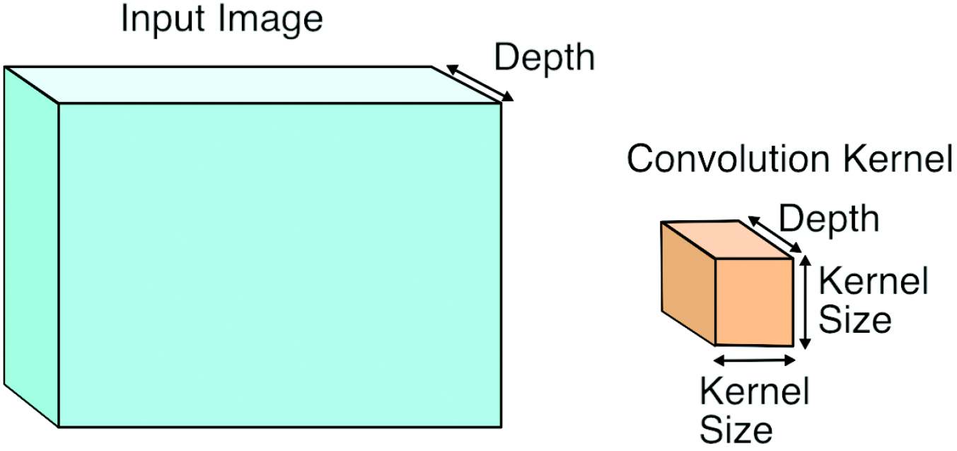
Matrix multiplication is a critical operation in many machine learning algorithms, particularly in the domain of deep learning. Training parameters (weights) of a deep neural network in a vectorized fashion essentially involves multiplication of matrices with various sizes.

Fully-Connected (FC) layers (Fig. 1(a)) and convolutional (Conv) layers (Fig. 1(b)) are building blocks of feed-forward and convolutional neural networks (Warden, 2015). It is straightforward to identify matrix multiplication in computing output value of a FC layer: each input has $k$ elements, and FC layer has $n$ neurons each with $k$ weights. An FC layer is the multiplication of a $m\times k$ matrix ($m$ is sample size) and a $k\times n$ matrix. A Conv layer appears to be a specialized operation, but it can be computed with matrix multiplication after rearranging data in a matrix format: each depth-wise (channel) slice of input can be added into an input matrix as a row; similarly each kernel can be added into a kernel matrix as a column. Convolution operation becomes multiplication of those two matrices. When using AlexNet on image classification with ImageNet dataset, vast majority of computation time on forward pass (94.7% on GPU, and 88.7% on CPU) is consumed by Conv and FC layers (Jia, 2014).

3.2 GEMM and Matrix Tiling

GEMM is a general procedure ubiquitously used in linear algebra, machine learning, statistics, and many other areas and is implemented in the BLAS (Basic Linear Algebra Subprograms) library (BLA, 2002). It multiplies two input matrices to produce an output matrix. The key difference between GEMM in deep learning and regular matrix multiplication is that the input matrices handled in deep learning are normally much larger. For example, a single layer in a typical convolution neural network may require multiplication of a $256\times 1024$ matrix by a $1024\times 128$ matrix to produce a $256\times 128$ matrix. Regular three-for-loop (Fig. 2) computation requires 34 million ($256\times 1024\times 128$) floating point operations (FLOPs). Modern deep neural networks may have hundreds of convolutional layers (e.g. ResNet152 (He et al., 2015)), and such networks may need several billions of FLOPs to finish operations in all layers for an input image.

Figure 2: Computing matrix multiplication

The time it takes to complete a GEMM computation largely depends on the cache hit rate of memory access. The large sizes of matrices usually forbid the entire matrices being loaded into memory or cache, however, GEMM can optimize memory access by iteratively splitting computation into smaller tiles, often referred to as the tiling process. A resulted matrix is initialized with zeros. GEMM uses outer products to compute part of a tile of the result and accumulates it on top of what has been stored in that tile. A tile is loaded from memory into cache and accumulates a new result on top of that. Fig. 3 (Matthes et al., 2017) illustrates a tiling strategy of GEMM.

Figure 3: An Example of Tiling Strategy

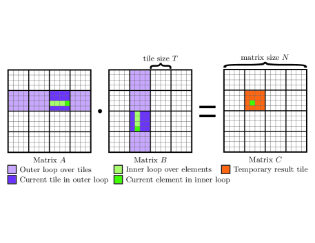
Original memory access patterns need to be transformed to adapt to the cache policy of a particular hardware. It is not straightforward to decide an optimal tiling strategy because it requires accurate estimate of accessed array regions in loops to match with cache size of target hardware and meet other constraints. An optimal tiling configuration chooses a tile size for each loop to collectively achieve the lowest running time on target hardware.

3.3 Problem Formulation

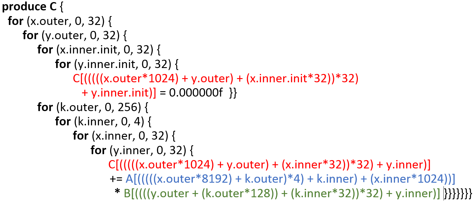
We use TVM (Chen et al., 2018a) to investigate the performance of matrix tiling for GEMM. TVM facilitates tiling optimization by generating Intermediate Representation (IR) of a particular configuration. Fig. 4 is a simple example IR of GEMM tiling configuration with a blocking factor of 32 on x86 CPU for GEMM with $(m=1024,k=1024,n=1024)$ (short as $(1024,1024,1024)$).

Figure 4: IR of GEMM with a blocking factor of 32

Definition: Generally, a GEMM tiling configuration can be defined as

$$\overrightarrow{\xi}=\overrightarrow{\xi_{m}}\times\overrightarrow{\xi_{k}}\times\overrightarrow{\xi_{n}},$$ (1)

where

$$\overrightarrow{\xi_{m}}=\{\left[m_{0},\ldots,m_{i},\ldots m_{d_{m}-1}\right]|\Pi_{i=0}^{d_{m}-1}m_{i}=m\},$$ (2)

$$\overrightarrow{\xi_{k}}=\{\left[k_{0},\ldots,k_{l},\ldots k_{d_{k}-1}\right]|\Pi_{l=0}^{d_{k}-1}k_{l}=k\},$$ (3)

$$\overrightarrow{\xi_{n}}=\{\left[n_{0},\ldots,n_{j},\ldots n_{d_{n}-1}\right]|\Pi_{j=0}^{d_{n}-1}n_{j}=n\}.$$ (4)

Multiplication of two matrices $A(m\times k)$ and $B(k\times n)$ produces matrix $C(m\times n)$. $d_{m}$, $d_{k}$ and $d_{n}$ are the number of nested loops for each dimension $m$, $k$ and $n$, respectively. $m_{i},k_{l},n_{j}$, $\forall i\in[0,d_{m})$ $\forall l\in[0,d_{k})$ $\forall j\in[0,d_{n})$, are the number of iterations of a respective loop. The configuration in Fig. 4 is $m_{0}=m_{1}=32$, $k_{0}=256,k_{1}=4$, $n_{0}=n_{1}=32$, and $d_{m}=d_{k}=d_{n}=2$.

We can formulate the optimal tiling configuration search problem into the following optimization problem:

$$\begin{array}[]{l}\mathop{\min}\limits_{s}~{}~{}{cost}(s;m,k,n,d_{m},d_{k},d_{n}).\end{array}$$

The objective is to find an optimal tiling configuration that has the minimal running time on target hardware. ${cost}$ denotes the running time for the configuration $s$, given the dimension of matrices ($m,k,n$) and the number of the nested loops on each dimension $d_{m}$, $d_{k}$, and $d_{n}$.

4 Methodology

In solving the formulated GEMM problem, the state-of-the-art XGBoost tuner (Chen et al., 2018b) has been shown to outperform the other classic tuners including random search and genetic algorithm based search. Nevertheless, training the XGBoost model for a large configuration space would incur a high cost. In this section, we propose two new tuning methods and a new configuration search model which allows exploitation of relations between similar configurations.

4.1 Configuration Search Modeling

We model the configuration tuning problem as a Markov Decision Process (MDP), where each configuration is regarded as a unique state. We define a state as follows.

$$s=\left[s_{m},s_{k},s_{n},J\right],$$ (5)

where $s_{m}=\left[m_{0},m_{1},\ldots,m_{d_{m}-1}\right]\in\xi_{m}$, $s_{k}=\left[k_{0},k_{1},\ldots,k_{d_{k}-1}\right]\in\xi_{k}$, $s_{n}=\left[n_{0},n_{1},\ldots,n_{d_{n}-1}\right]\in\xi_{n}$, and $J$ is a binary number indicating whether the state is legitimate.

As in the GEMM application, with similar configuration settings, i.e., the configuration parameters for each dimension of two states are equal or close, the performance of thw two states is more likely to be similar. Taking advantage of the relationship between similar configurations, and considering the constraints of the matrix size in each configuration. We define the action space as follows,

$$\mathcal{A}=\emph{\{}{s_{x}[i]\leftarrow 2s_{x}[i]~{}~{}\text{and}~{}~{}s_{x}[j]\leftarrow s_{x}[j]/2}\emph{\}},$$ (6)

where $\forall x\in\{m,k,n\},\forall i,j\in[0,d_{x}),~{}\text{and}~{}i\neq j$.

Accordingly, we define a step function $step$ as the transition from one state to another,

$$s^{\prime}=step(s,a).$$ (7)

With the input of a particular action $a\in\mathcal{A}$, the current state $s$ transitions to state $s^{\prime}$.

Figure 5: G-BFS Method: (a) Flow chart; (b) Illustration; (c) Sample search trajectory

In addition, if the agent takes action $a$ and transitions from state $s$ to state $s^{\prime}$, we define the reward function as follows,

$$r(s,a)=\frac{1}{{cost}(s^{\prime};m,k,n,d_{m},d_{k},d_{n})}.$$ (8)

Following MDP model, the agent is expected to determine its policy $\boldsymbol{\pi}$ so as to efficiently approach and discover a state $s^{*}$ with the lowest running time in the target hardware system.

In the following subsections, we will propose two different configuration tuning approaches based on the configuration search model, guided by G-BFS and N-A2C reinforcement learning, respectively, followed by a discussion of their strengths in different scenarios.

4.2 G-BFS Method

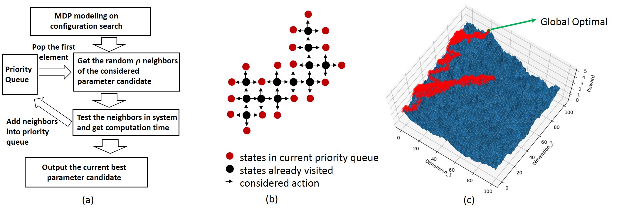
The G-BFS method is guided by Greedy Best-First-Search and follows the flowchart in Fig. 5(a). We initialize an empty priority queue $\mathcal{Q}$ (ordered by increasing cost), an empty list $S_{v}$ to record all visited states, and a random or hand-crafted starting state $s_{0}$. We first test (i.e., run the configuration on target hardware) and enque the starting state $s_{0}$ and record its running time ${cost}(s_{0})$ into the priority queue $\mathcal{Q}$. In each iteration, we deque the top configuration candidate $s$ from $\mathcal{Q}$, iterate through all actions $a\in\mathcal{A}$, and collect all corresponding neighbor states as

$$g(s)=[s^{\prime}=step(s,a)~{}~{}\forall a\in\mathcal{A}].$$ (9)

We randomly select $\rho$ ($\rho\in\{1,2,\ldots,len(g(s))\}$) states from $g(s)$, and test them in hardware. For each state $s^{\prime}$ from $g(s)$, if $s^{\prime}$ is legitimate and has not been visited before, we enque $s^{\prime}$ and its running time ${cost}(s^{\prime})$ into $\mathcal{Q}$ and add state $s^{\prime}$ in the visited list $S_{v}$. If its running time ${cost}(s^{\prime})$ is smaller than the current minimum running time, we set state $s^{\prime}$ as the optimal state visited and record its running time as ${cost}_{min}$. The iteration continues until the priority queue is empty or the search time reaches the maximum time $T_{max}$ specified by the user. The current optimal state $s^{*}$ and its running time ${cost}_{min}$ are returned as tuning results. The summary of the algorithm is shown in Algorithm 1.

Algorithm 1 G-BFS Method

 

1:  Initialization: $\mathcal{Q}$=PriorityQueue(), $S_{v}$, $s_{0}$

2:  $\mathcal{Q}$.push($({cost}(s_{0}),s_{0})$);

3:  Add $s_{0}$ in $S_{v}$;

4:  while $\mathcal{Q}\neq\O$ and $t_{search}<T_{max}$ do

5:     $({cost}(s),s)$ = $\mathcal{Q}$.pop();

6:     $\mathcal{B}$ = Take $\rho$ neighbors randomly from $g(s)$;

7:     for $s^{\prime}$ in $\mathcal{B}$ do

8:        if $s^{\prime}$ is legitimate and $s^{\prime}\not\in S_{v}$ then

9:           $\mathcal{Q}$.push($({cost}(s^{\prime}),s^{\prime})$);

10:           Add $s^{\prime}$ in $S_{v}$;

11:           if ${cost}_{min}>{cost}(s^{\prime})$ then

12:              ${cost}_{min}={cost}(s^{\prime})$;

13:              $s^{*}=s^{\prime}$;

14:           end if

15:        end if

16:     end for

17:  end while

18:  Return: Configuration $s^{*}$ with ${cost}_{min}$.

 

In Fig. 5(b), we illustrate the exploration in the middle of the tuning process, where the red nodes denote the state currently stored in the priority queue and the grey nodes are the visited states. In subsequent iterations, the method will explore from the $\rho$ most promising red nodes. In Fig. 5(c), we depict an example of 2-dimensional configuration search with a randomly generated reward function. The proposed G-BFS method is able to correct itself from exploring wrong directions and efficiently expand its neighborhood to the optimal states. Moreover, when $\rho=len(g(s))$, given unlimited tuning time, the algorithm is guaranteed to visit all configuration states.

4.3 N-A2C Method

As the G-BFS method explores only one step from the considered state for each iteration, its performance may be affected when the cost from similar states exhibits large random noise. In the N-A2C method, as shown in Fig. 6(a), for each episode, we explore in a $\varsigma$-step neighborhood, and the direction of exploration is guided by the A2C method (Bhatnagar et al., 2009). The center of the exploration neighborhood is periodically updated with the optimal states ever visited.

We summarize the N-A2C method in Algorithm 2. We initialize a random or hand-crafted starting state $s_{0}$, a fixed-size memory buffer $\mathcal{M}$ to record the latest search information, and an empty hashtable $H_{v}$ to record all visited states with the associated cost. For the A2C model, both actor and critic initialize their neural networks with random weights. In each episode, from the same starting point, the agent explores $\mathcal{T}$ continuous steps. For each step, the agent follows the $\epsilon$-greedy algorithm, where with probability of $\epsilon$, the agent takes action $a$ guided by the policy $\pi(s)$ generated by the actor’s neural network; and with probability of $1-\epsilon$, the agent chooses a random action $a$ from the current state. Based on the current state $s$ and action $a$, we get the next state $s^{\prime}$ from Eqn. 7. If the next state $s^{\prime}$ has not been visited before, we add $s^{\prime}$ into collected candidate set $\mathcal{B}_{collect}$. The process iterates until the number of collected states reaches the predefined threshold, and the hardware executes the GEMM computation code generated with the collected configuration candidates. The hashmap $H_{v}$ and memory buffer $\mathcal{M}$ are then updated with the configuration candidates and the associated running time. The exploration data stored in $\mathcal{M}$ is used to incrementally-train the neural networks of A2C.

Figure 6: N-A2C Method: (a) Flow chart; (b) Illustration; (c) Sample search trajectory

Algorithm 2 N-A2C Method

 

1:  Initialization: $s_{0}$, $\mathcal{M}$, $H_{v}$, ${cost}_{min}$

2:  for each episode do

3:     while $len(\mathcal{B}_{collect})<len(\mathcal{B}_{test})$  do

4:        $s=s_{0}$;

5:        for each step until $\mathcal{T}$ steps do

6:           if $rand()<\epsilon$ then

7:              $a$ follows $\pi(s)$;

8:           else

9:              $a$ is randomly selected from $\mathcal{A}$;

10:           end if

11:           $s^{\prime}=step(s,a)$;

12:           if $s^{\prime}$ not in $H_{v}$ then

13:              Add $s^{\prime}$ in $\mathcal{B}_{collect}$;

14:           end if

15:           $s=s^{\prime}$;

16:        end for

17:     end while

18:     for $s^{\prime}$ in $\mathcal{B}_{collect}$ do

19:        if ${cost}_{min}>{cost}(s^{\prime})$ then

20:           ${cost}_{min}={cost}(s^{\prime})$;

21:           $s^{*}=s^{\prime}$;

22:           $s_{0}=s^{*}$;

23:        end if

24:        $H_{v}[s^{\prime}]={cost}(s^{\prime})$;

25:        Store $(s,a,r(s,a),s^{\prime})$ to $\mathcal{M}$, where $\forall s$, $\forall a$ satisfying $step(s,a)=s^{\prime}$;

26:        Train actor’s and critic’s neural networks with $\mathcal{M}$;

27:     end for

28:  end for

29:  Return: Configuration $s^{*}$ with ${cost}_{min}$.

 

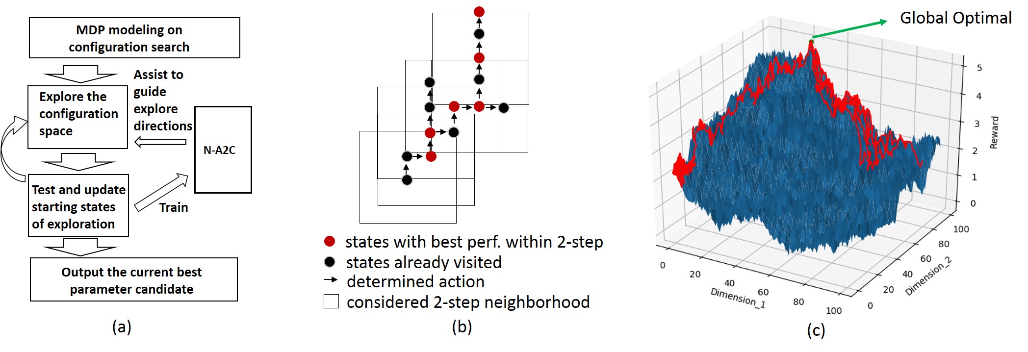
Generally, the proposed N-A2C method is able to efficiently search the optimal GEMM configuration with fixed exploration steps in each episode. Nevertheless, heuristics can be applied. Just like learning-rate decay in training deep neural networks, the exploration step $\mathcal{T}$ can have a decay process, i.e., starting with a large value and gradually reducing to a small number. In addition, the exploration step $\mathcal{T}$ can also increase to explore new configuration neighborhoods.

In Fig. 6(b), we depict a simple exploration map with the proposed N-A2C method and $\mathcal{T}=2$. Unlike Fig. 5(b), the exploration neighborhood is defined as two steps from current states. In Fig. 6(c), we show an example of 2-dimensional configuration with a randomly generated reward function. Due to the large randomness in the example, we set the exploration step $\mathcal{T}$ as 100 and the global optimal state is efficiently discovered with the guidance of the A2C algorithm.

5 Experimental Results

(a) Optimal running time vs. fraction of explored configuration space

(b) Optimal running time vs. searching time

Figure 7: Comparison of GEMM tuning for (1024, 1024, 1024)

We evaluate the performance of the proposed GEMM configuration tuning approaches on Nvidia Titan Xp GPU in the TVM framework. Following similar settings in TVM for GPUs, we set the number of nested loops for each dimension as $d_{m}=4,d_{k}=2,d_{n}=4$. We set the random selection parameter $\rho=5$ for the G-BFS method, and the maximum number of search steps $\mathcal{T}=3$ for the N-A2C method. Without losing generality, we set the initial state for both methods as $s_{0}=[[m,1,1,1],[k,1],[n,1,1,1]]$, which represents the configuration without multi-level matrix tiling. The performance of the proposed methods can be further improved by setting the initial state to a more meaningful configuration. In order to investigate the performance of the proposed methods, we compare them with state-of-the-art algorithms including the XGBoost method (Chen et al., 2018b) in TVM framework and the general configuration optimization method using a RNN controller by Google researchers. Unless otherwise specified, the computation time for each configuration is the arithmetic mean for 10 repeated trials on the tested GPU hardware.

Without losing their applicability to deep learning, we evaluate the four approaches on a perceptron network, which is the fundamental building block for state-of-the-art neural network architectures while mainly including GEMM for computation. We denotes the computation in the perceptron network as $\mathbf{Y}=\mathbf{W^{T}}\mathbf{X}$, where $\mathbf{W}\in\mathbb{R}^{(k,m)},\mathbf{X}\in\mathbb{R}^{(k,n)}$, and $\mathbf{Y}\in\mathbb{R}^{(m,n)}$; $n$ is the batch size, $k$ is the input dimension, and $m$ is the output dimension. Accordingly, we denote the size of perceptron network in the format of $(m,k,n)$, which corresponds to matrices $A(m\times k)$ and $B(k\times n)$ for GEMM.

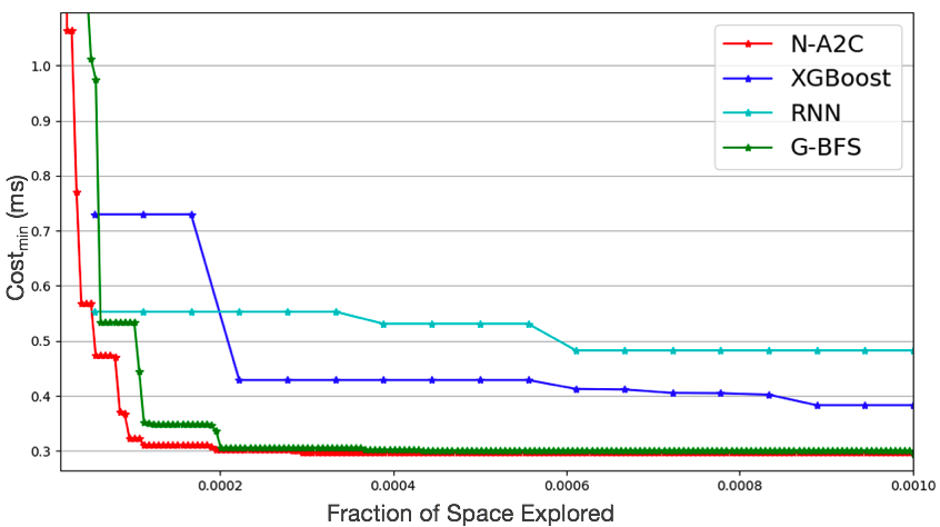
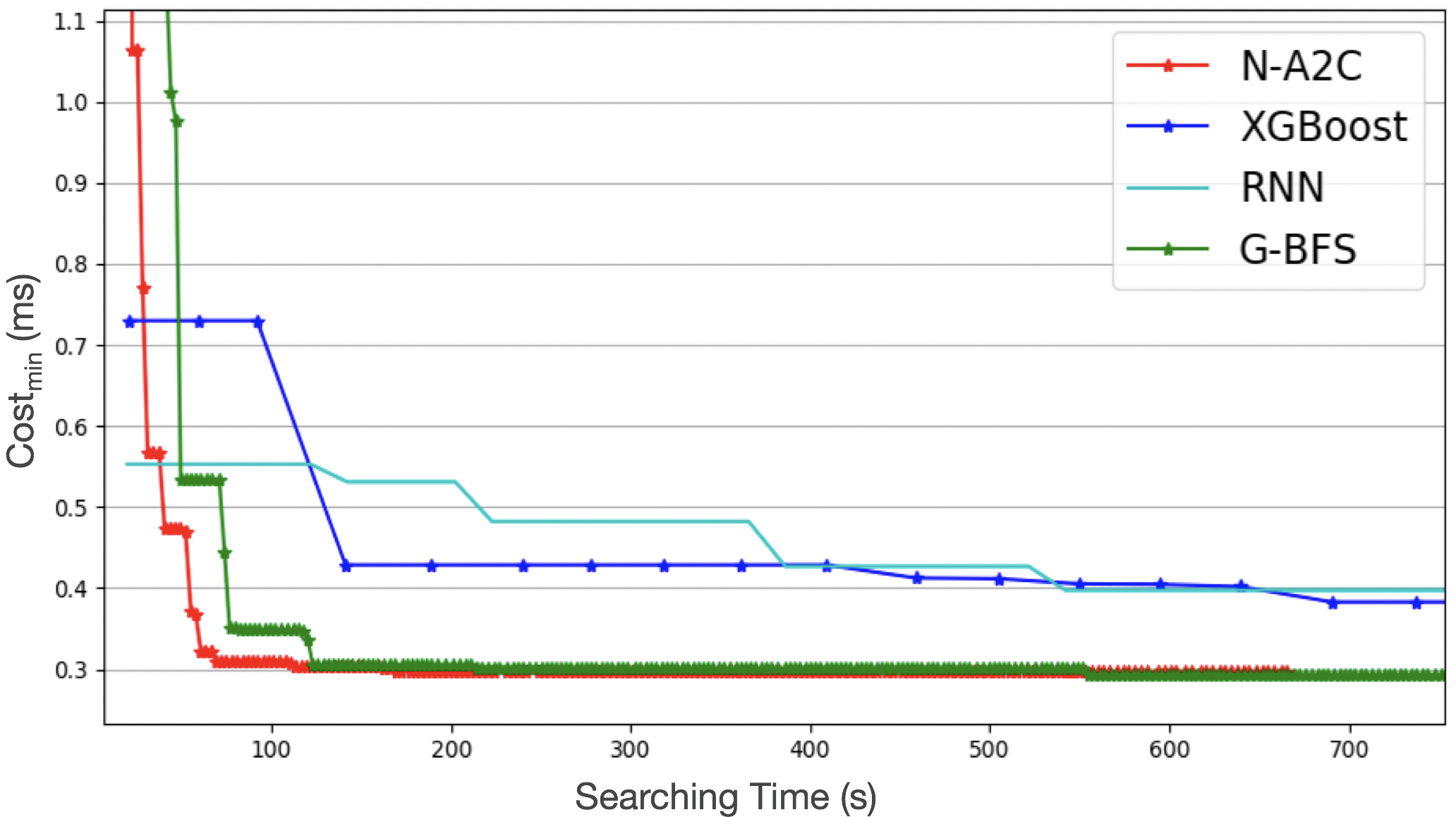
In Fig. 7, we set input dimension as $1024$, batch size as $1024$ and output dimension as $1024$. We first evaluate the optimal computation time discovered with respect to the fraction of visited configurations in Fig. 7(a). Based on the sizes of matrices and the number of nested loops, there are $899756$ configuration candidates. With increasing fraction of visited configurations, the optimal cost in terms of hardware computation time discovered generally decreases. Compared with the XGBoost and RNN methods, the proposed N-A2C and G-BFS methods are able to discover the better configurations with lower fraction of visited configuration candidates. Fig. 7(b) plots the optimal cost discovered by four methods over time. It generally takes the proposed N-A2C and G-BFS methods less time to find the configuration with lower cost, compared with the XGBoost and RNN methods.

(a) Visited configurations = 0.1%

(b) Searching time = 750 seconds

Figure 8: Performance comparison of tuners

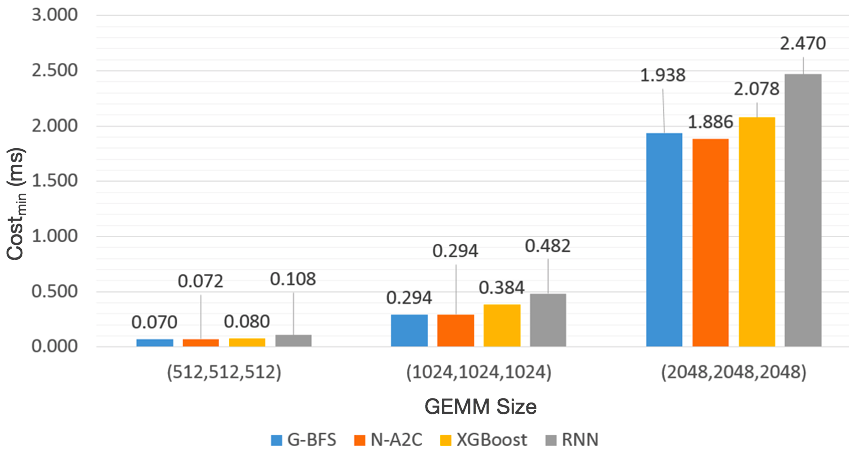
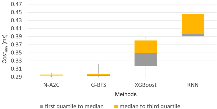
In Fig. 8, we evaluate and compare the configuration tuning efficiency in the perceptron network. In Fig. 8(a), we compare the discovered optimal computation time when the fraction of visited configuration candidates reaches 0.1%. The total numbers of configuration candidates for $(512,512,512)$, $(1024,1024,1024)$, $(2048,2048,2048)$ matrix tiling are $484000$, $899756$, and $1589952$, respectively. As the sizes of matrices increase, longer computation time is required, and G-BFS and N-A2C can search configuration more efficiently than the XGBoost and RNN methods. Specifically, with 0.1% exploration of $(1024,1024,1024)$’s configuration space, the proposed G-BFS and N-A2C methods are able to discover configurations of 24% lower cost (computation time) than what the XGBoost method can find and configurations of 40% lower cost than what the RNN method can find. The N-A2C method outperform the G-BFS method for larger matrix sizes (e.g. $(2048,2048,2048)$), as the N-A2C method is able to go multiple steps from the current state. In Fig. 8(b), we compare the cost of best configuration discovered when the tuning time is limited to 750 seconds. In order to show the variance of performance incurred by random exploration for each method, we use a box plot with the minimum, first quartile, median, mean, third quartile, and maximum values for 10 trials on the $(1024,1024,1024)$ tiling. Our methods not only achieve better mean and median results, but also exhibit more stable behaviors (less variance) than the other two methods.

6 Conclusion

In this paper, we propose a Greedy Best First Search (G-BFS) method and a Neighborhood Actor Advantage Critic (N-A2C) method for compiler-level GEMM optimization, taking advantage of performance of neighborhood configurations. The G-BFS method, though being lightweight, outperforms the XBboost and RNN methods consistently; and the N-A2C method performs even better for large matrices. Empirical results show that both methods achieve significant performance improvement over state-of-the-art tuning methods such as those using XGBoost and RNN controller. Both methods are general in the sense that they are applicable to other compiler-level tuning tasks and can be used for optimization of other tensor operators with large configuration space.

References

- BLA (2002) An updated set of basic linear algebra subprograms (blas). ACM Trans. Math. Softw., 28(2):135–151, June 2002. ISSN 0098-3500. doi: 10.1145/567806.567807. URL http://doi.acm.org/10.1145/567806.567807.
- Bellman (1961) Bellman, R. E. Adaptive control processes: a guided tour. Princeton university press, 1961.
- Bello et al. (2017) Bello, I., Zoph, B., Vasudevan, V., and Le, Q. V. Neural optimizer search with reinforcement learning. arXiv preprint arXiv:1709.07417, 2017.
- Bergstra & Bengio (2012) Bergstra, J. and Bengio, Y. Random search for hyper-parameter optimization. Journal of Machine Learning Research, 13(Feb):281–305, 2012.
- Bergstra et al. (2011) Bergstra, J. S., Bardenet, R., Bengio, Y., and Kégl, B. Algorithms for hyper-parameter optimization. In Advances in neural information processing systems, pp. 2546–2554, 2011.
- Bhatnagar et al. (2009) Bhatnagar, S., Sutton, R. S., Ghavamzadeh, M., and Lee, M. Natural actor–critic algorithms. Automatica, 45(11):2471–2482, 2009.
- Bosman et al. (2007) Bosman, P. A. N., Grahl, J., and Thierens, D. Adapted maximum-likelihood gaussian models for numerical optimization with continuous edas. Software Engineering [SEN], (E0704), 2007.
- Chen & Guestrin (2016) Chen, T. and Guestrin, C. Xgboost: A scalable tree boosting system. In Proceedings of the 22nd acm sigkdd international conference on knowledge discovery and data mining, pp. 785–794. ACM, 2016.
- Chen et al. (2018a) Chen, T., Moreau, T., Jiang, Z., Shen, H., Yan, E. Q., Wang, L., Hu, Y., Ceze, L., Guestrin, C., and Krishnamurthy, A. TVM: end-to-end optimization stack for deep learning. 2018a. URL http://arxiv.org/abs/1802.04799.
- Chen et al. (2018b) Chen, T., Zheng, L., Yan, E. Q., Jiang, Z., Moreau, T., Ceze, L., Guestrin, C., and Krishnamurthy, A. Learning to optimize tensor programs. 2018b. URL http://arxiv.org/abs/1805.08166.
- Chetlur et al. (2014) Chetlur, S., Woolley, C., Vandermersch, P., Cohen, J., Tran, J., Catanzaro, B., and Shelhamer, E. cudnn: Efficient primitives for deep learning. arXiv preprint arXiv:1410.0759, 2014.
- Das et al. (2016) Das, D., Avancha, S., Mudigere, D., Vaidynathan, K., Sridharan, S., Kalamkar, D., Kaul, B., and Dubey, P. Distributed deep learning using synchronous stochastic gradient descent. arXiv preprint arXiv:1602.06709, 2016.
- Dukhan (2016) Dukhan, M. Nnpack, 2016.
- Goldberg (1989) Goldberg, D. E. Genetic Algorithms in Search, Optimization and Machine Learning. Addison-Wesley Longman Publishing Co., 1989.
- Hansen & Ostermeier (2001) Hansen, N. and Ostermeier, A. Completely derandomized self-adaptation in evolution strategies. Evolutionary computation, 9(2):159–195, 2001.
- He et al. (2015) He, K., Zhang, X., Ren, S., and Sun, J. Deep residual learning for image recognition. In arXiv prepring arXiv:1506.01497, 2015.
- Hinton (2012) Hinton, G. E. A practical guide to training restricted boltzmann machines. In Neural networks: Tricks of the trade, pp. 599–619. Springer, 2012.
- Hoffman & Shahriari (2014) Hoffman, M. W. and Shahriari, B. Modular mechanisms for bayesian optimization. In NIPS Workshop on Bayesian Optimization, pp. 1–5. Citeseer, 2014.
- Holland (1975) Holland, J. H. Adaptation in Natural and Artificial Systems. The University of Michigan Press, 1975.
- Hutter et al. (2011) Hutter, F., Hoos, H. H., and Leyton-Brown, K. Sequential model-based optimization for general algorithm configuration. In International Conference on Learning and Intelligent Optimization, pp. 507–523. Springer, 2011.
- Jia (2014) Jia, Y. Learning Semantic Image Representations at a Large Scale. PhD thesis, Univ. of California at Berkeley, Berkely, Calif., 2014.
- Kandasamy et al. (2018) Kandasamy, K., Neiswanger, W., Schneider, J., Poczos, B., and Xing, E. Neural architecture search with bayesian optimisation and optimal transport. arXiv preprint arXiv:1802.07191, 2018.
- Kennedy et al. (2001) Kennedy, J., Eberhart, R. C., and Shi, Y. Swarm intelligence. 2001. Kaufmann, San Francisco, 1:700–720, 2001.
- Larochelle et al. (2007) Larochelle, H., Erhan, D., Courville, A., Bergstra, J., and Bengio, Y. An empirical evaluation of deep architectures on problems with many factors of variation. In Proceedings of the 24th international conference on Machine learning, pp. 473–480. ACM, 2007.
- Larrañaga & Lozano (2001) Larrañaga, P. and Lozano, J. A. Estimation of distribution algorithms: A new tool for evolutionary computation, volume 2. Springer Science & Business Media, 2001.
- Leary & Wang (2017) Leary, C. and Wang, T. Xla: Tensorflow, compiled. TensorFlow Dev Summit, 2017.
- LeCun et al. (2015) LeCun, Y., Bengio, Y., and Hinton, G. Deep learning. nature, 521(7553):436, 2015.
- LeCun et al. (2012) LeCun, Y. A., Bottou, L., Orr, G. B., and Müller, K.-R. Efficient backprop. In Neural networks: Tricks of the trade, pp. 9–48. Springer, 2012.
- Loshchilov & Hutter (2016) Loshchilov, I. and Hutter, F. CMA-ES for hyperparameter optimization of deep neural networks. CoRR, abs/1604.07269, 2016. URL http://arxiv.org/abs/1604.07269.
- Matthes et al. (2017) Matthes, A., Widera, R., Zenker, E., Worpitz, B., Huebl, A., and Bussmann, M. Tuning and optimization for a variety of many-core architectures without changing a single line of implementation code using the alpaka library. Technical report, https://arxiv.org/abs/1706.10086, 2017.
- Mirhoseini et al. (2017) Mirhoseini, A., Pham, H., Le, Q. V., Steiner, B., Larsen, R., Zhou, Y., Kumar, N., Norouzi, M., Bengio, S., and Dean, J. Device placement optimization with reinforcement learning. arXiv preprint arXiv:1706.04972, 2017.
- NNVM (2017) NNVM. Nnvm compiler: Open compiler for ai frameworks. 2017. URL http://tvmlang.org/2017/10/06/nnvm-compiler-announcement.html.
- Pham et al. (2018) Pham, H., Guan, M. Y., Zoph, B., Le, Q. V., and Dean, J. Efficient neural architecture search via parameter sharing. arXiv preprint arXiv:1802.03268, 2018.
- Ragan-Kelley et al. (2013) Ragan-Kelley, J., Barnes, C., Adams, A., Paris, S., Durand, F., and Amarasinghe, S. Halide: a language and compiler for optimizing parallelism, locality, and recomputation in image processing pipelines. ACM SIGPLAN Notices, 48(6):519–530, 2013.
- Ramachandran et al. (2018) Ramachandran, P., Zoph, B., and Le, Q. V. Searching for activation functions. 2018.
- Rechenberg & Eigen (1973) Rechenberg, I. and Eigen, M. Evolutionsstrategie: Optimierung technischer systeme nach prinzipien der biologischen evolution. Frommann-Holzboog Verlag, Stuttgart, 1973.
- Schwefel (1977) Schwefel, H.-P. Numerische Optimierung von Computer-Modellen mittels der Evolutionsstrategie: mit einer vergleichenden Einführung in die Hill-Climbing-und Zufallsstrategie. Birkhäuser, 1977.
- Snoek et al. (2012) Snoek, J., Larochelle, H., and Adams, R. P. Practical bayesian optimization of machine learning algorithms. In Advances in neural information processing systems, pp. 2951–2959, 2012.
- Storn & Price (1997) Storn, R. and Price, K. Differential evolution – a simple and efficient heuristic for global optimization over continuous spaces. Journal of Global Optimization, 11(4):341–359, Dec 1997. ISSN 1573-2916. doi: 10.1023/A:1008202821328. URL https://doi.org/10.1023/A:1008202821328.
- Truong et al. (2016) Truong, L., Barik, R., Totoni, E., Liu, H., Markley, C., Fox, A., and Shpeisman, T. Latte: a language, compiler, and runtime for elegant and efficient deep neural networks. ACM SIGPLAN Notices, 51(6):209–223, 2016.
- Warden (2015) Warden, P. Why gemm is at the heart of deep learning? https://petewarden.com/2015/04/20/why-gemm-is-at-the-heart-of-deep-learning/, 2015.
- Wierstra et al. (2014) Wierstra, D., Schaul, T., Glasmachers, T., Sun, Y., Peters, J., and Schmidhuber, J. Natural evolution strategies. The Journal of Machine Learning Research, 15(1):949–980, 2014.
- Zoph & Le (2016) Zoph, B. and Le, Q. V. Neural architecture search with reinforcement learning. arXiv preprint arXiv:1611.01578, 2016.