Mobility edge of the two dimensional Bose-Hubbard model
Abstract
We analyze the disorder driven localization of the two dimensional Bose-Hubbard model by evaluating the full low energy quasiparticle spectrum via a recently developed fluctuation operator expansion method. For any strength of the local interaction we find a mobility edge that displays an approximately exponential decay with increasing disorder strength. We determine the finite-size scaling collapse and exponents at this critical line finding that the localization of excitations is characterized by weak multi-fractality and a thermal-like critical gap ratio. A direct comparison to a recent experiment yields an excellent match of the predicted finite-size transition point and scaling of single particle correlations.
pacs:
67.85.De, 03.75.Lm, 05.30.Jp, 63.20.PwI Introduction
In the last decade the study of disorder-driven localization of quantum particles has received considerable interest, following the suggestion that Anderson localization for non-interacting models Anderson (1958); Abrahams et al. (1979); Fleishman and Anderson (1980); Roati et al. (2008) can be generalized to interacting ones Altshuler et al. (1997); Basko et al. (2006); Oganesyan and Huse (2007); Pal and Huse (2010) in the framework of the so-called many-body localization (MBL). One of the most prominent features of MBL is its incompatibility with the eigenstate thermalization hypothesis (ETH) resulting from an extensive number of local integrals of motion Serbyn et al. (2013); Huse et al. (2014); Chandran et al. (2015); Ros et al. (2015); Imbrie et al. (2017). A complete demonstration of MBL would in principle require knowledge of the whole spectrum, limiting the use of exact diagonalization techniques to small system sizes, especially when bosonic particles are considered Sierant and Zakrzewski (2018); Wahl et al. (2019). The existence of MBL has been rigorously proven in one-dimensional (1D) spin-chains Imbrie (2016a, b), while various perturbative arguments Fleishman and Anderson (1980); Altshuler et al. (1997); Basko et al. (2006); Nandkishore (2014) and numerical evidence Oganesyan and Huse (2007); Pal and Huse (2010); Kshetrimayum et al. (2019) have also supported its existence in two dimensions - involving a mobility edge (ME) separating mobile from localized states in the spectrum. However, recent theoretical arguments have challenged the existence of MBL both in 1D Šuntajs et al. (2019) and 2D De Roeck et al. (2016); Agarwal et al. (2017); De Roeck and Huveneers (2017) in the thermodynamic limit. Experimental realizations of bosonic systems have already been achieved in cold atom setups where a disorder potential can be imprinted onto a confined optical lattice in 1D Lukin et al. (2019); Rispoli et al. (2019) and 2D Choi et al. (2016); Rubio-Abadal et al. (2019), showing strong signs of high energy localization in confined systems for both cases. Related experiments Fallani et al. (2007); Meldgin et al. (2016) have also observed evidence for a ground state Bose-glass phase compatible with theoretical predictions of a zero-energy superfluid to Bose-glass transition Fisher et al. (1989); Makivić et al. (1993); Zhang et al. (1995); Priyadarshee et al. (2006); Söyler et al. (2011); Álvarez Zúñiga and Laflorencie (2013); Saliba et al. (2014); Álvarez Zúñiga et al. (2015).
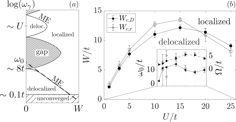
Here, we investigate localization effects in the excitation spectrum of the two-dimensional Bose-Hubbard model (BHM) in the presence of disorder utilizing a recently developed fluctuation operator expansion (FOE) method Bissbort et al. (2014); Geißler et al. (2018), which gives access to the complete spectrum of quasiparticle (QP) excitations for system sizes comparable to experiments. Our results are summarized in Fig. 1. For all interaction strengths disorder induces (at least) one ME. We determine the finite-size scaling at the critical points characterized by weak fractality and a thermal-like critical gap ratio. Importantly, in the limits of our numerical QP method the low energy ME converges onto an exponential decay with disorder. For the case of particles confined by a harmonic potential, we compute correlation functions and extract the inverse decay length, finding excellent agreement with recent experiments Choi et al. (2016) in terms of a finite-size localization transition.
In the following we first introduce the model (Set. II) and the fluctuation operator expansion (Sec. III). In Sec. IV we introduce the observables used to characterize localization and discuss their finite-size collapse determining the ME (Sec. IV.1). We determine the finite-size localization transition of a harmonically trapped system (Sec. V) and directly compare to the experimental results of reference Choi et al. (2016). In Sec. VI finally, we end with some concluding remarks.
II Model
The Hamiltonian of the BHM with on-site disorder and in the grand canonical ensemble reads
| (1) |
where are bosonic creation (annihilation) operators at the site , is the tunneling rate between nearest neighbor sites on a square lattice of spacing and linear size , while is the local on-site Hubbard interaction. The energy reads , with the chemical potential fixing the particle number and a local energy shift due to disorder or an external harmonic potential. With Ref. Choi et al. (2016) in mind we choose a Gaussian probability distribution with the standard deviation 111A crucial difference compared to the commonly considered box disorder is the presence of rare extreme peaks or wells in the potential.. In this work we analyze this model over a range of interactions and disorder strengths at half-filling. We furthermore investigate the effect of an external trapping potential in order to compare with the recent experiment Choi et al. (2016) for and .
III Fluctuation operator expansion
The FOE Bissbort et al. (2014); Geißler et al. (2018) is a QP method based on a Gutzwiller expansion of (1) in terms of eigenstates of the local mean-field Hamiltonians , where the fluctuation operators and the fields are determined self-consistently. For , constitutes an exact quadratic map onto a complete basis set of the local Gutzwiller raising (lowering) operators (). These generate arbitrary local fluctuations of any self-consistent MF state . The quality of the approximation is ascertained for (in this work we always find this criterion to be fulfilled in the quasiparticle ground state (5) 222We refer the interested reader to our follow-up work Geißler (2020) for a detailed discussion of the FOE method in the context of disordered systems.). Here, we consider terms of second order in the Gutzwiller operators, which using yields the following approximate representation of 333We note that the MF self-consistency condition guarantees the absence of first order terms.
| (2) |
The scalar term results from reordering normal ordered terms to anti-normal order, while the matrix entries are given by the local matrix elements ,
| (3) | ||||
| (4) |
Here, is the tunneling matrix with nonzero entries only for neighboring sites, and are the local excitation energies of the th Gutzwiller excitation at site .
The diagonalization of (2) yields in terms of infinitely lived QP modes with corresponding energies and are the generalized Bogoliubov-type operators, with and the corresponding eigenvectors. Analogous to standard Bogoliubov theory, these inherit approximately bosonic commutation relations from the Gutzwiller operators for . and can be interpreted as dual wave-functions analogous to particle and hole fluctuations. Normal ordering of operators results in a scalar correction , irrelevant to the present discussion Geißler et al. (2018). Finally, we implicitly define the QP ground state via
| (5) |
which also best fulfills the approximation of neglected QP interactions Bissbort et al. (2014); Geißler et al. (2018).
Drawing from variational concepts Huber et al. (2007, 2008); Bissbort et al. (2011); Endres et al. (2012) and based on a MF description that becomes exact for weak and strong interactions, the FOE allows for a systematic, non-perturbative improvement over standard Bogoliubov theory Bogolyubov (1947) that also incorporates effects of many-body entanglement 444See Supplemental Material at [] for a discussion of details of the finite-size scaling analysis for the excitations and the ground state, a comparison of scenarios for the decay of correlations in a trapped system and a discussion of the entanglement captured by the FOE method.. It gives access to the otherwise neglected gapped (amplitude) Hubbard subbands in the disorder-free limit of in Eq. (1) Bissbort et al. (2014); Geißler et al. (2018). As we show in the following sections, these modes, absent in standard Bogolioubov theory, play an important role in the localization transition at finite energy. We note that Bogoliubov quasiparticle theory has already been used to successfully investigate 2D localization at low energy (e.g. Álvarez Zúñiga and Laflorencie (2013); Saliba et al. (2014); Gaul et al. (2015)), and in particular the existence of a Bose-Glass phase for hard-core bosons (i.e., ) with binary disorder Álvarez Zúñiga and Laflorencie (2013). Numerous works have unambiguously demonstrated the existence of a direct zero-energy phase transition between a Bose condensed superfluid and a Bose-Glass for the 2D BHM with uniform disorder distribution, similar to Eq. (1) Fisher et al. (1989); Makivić et al. (1993); Zhang et al. (1995); Priyadarshee et al. (2006); Álvarez Zúñiga et al. (2015). Here we focus on the existence of a finite-energy ME.
IV Localization characteristics
To characterize the degree of localization we consider the following two observables: (i) The gap ratio
| (6) |
with the quasiparticle energy gaps and the disorder average. The observable is known from random matrix theory Oganesyan and Huse (2007); Atas et al. (2013) to have the mean value and in the delocalized and localized phases, respectively, resulting from level statistics belonging to the Gaussian orthogonal and Poisson ensembles. The second observable is (ii) the fractal dimension of the QP fluctuation wave-functions . Analogous to the scaling of -moments of many-body eigenstates Hentschel and Procaccia (1983); Macé et al. (2019); Lindinger et al. (2019) we define
| (7) |
for the local amplitudes of the wave-function, which naturally characterize the spatial extension of each QP mode [see examples in Fig. 2(a)]. For our purposes we consider , while one obtains the multifractality spectrum by also taking all other values into account.
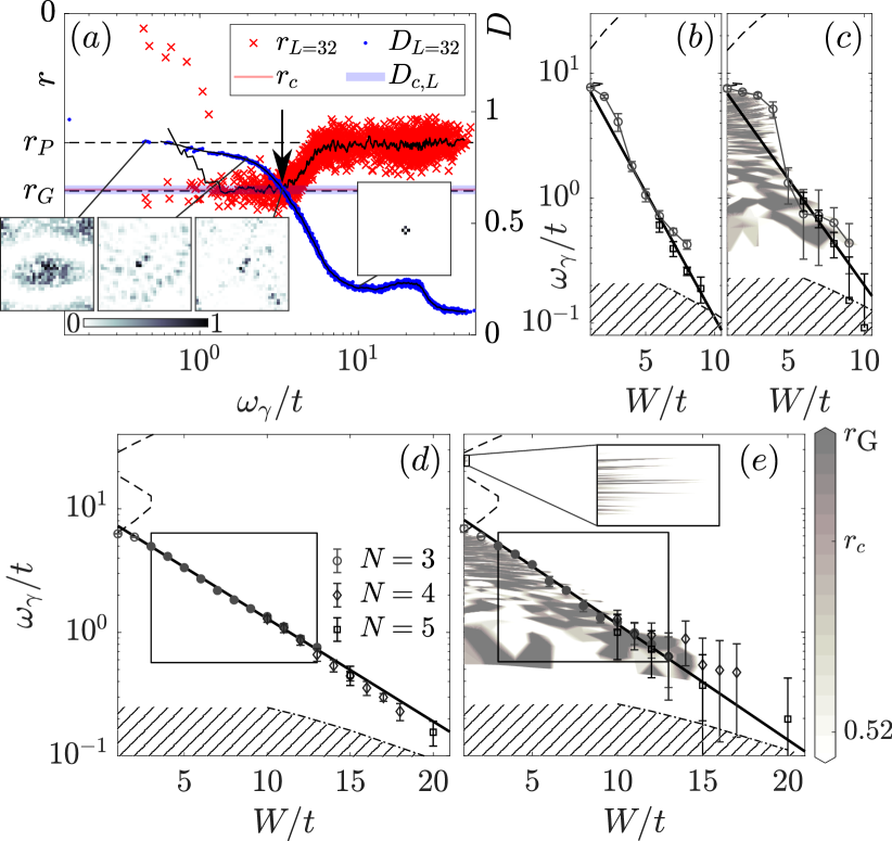
Delocalized states with 555From here on we omit the indices of the observables unless they are necessary. appear primarily at low QP energies and for weak disorder , as shown in the contour plots Fig. 2 for weak () and strong () interactions, respectively. We note that values of for weak disorder and small QP energies [e.g. for in Fig. 2()] result from symmetry related finite-size effects irrelevant to our discussion.
For and we find a band of additional delocalized states for energies reflecting the presence of typical Hubbard subbands which overlap for [dashed lines in Fig. 2]. In all cases, increasing spreads the bands so they overlap and drives a transition to localized states with , implying the existence of (multiple) MEs. For the same cases we find similar behavior for the fractal dimension down to the truncation limit [compare Fig. 2]. Data points in Figs. 2 mark the MEs determined via a finite-size scaling as discussed in the next section.
IV.1 Finite-size scaling analysis
We determine the position of the (lowest energy) ME via finite-size scaling for the case , with linear sizes and corresponding numbers of realizations for which we find to be sufficient here Note (4). We find the data to be consistent with the scaling relations
| (8) | ||||
| (9) |
Here, and are the scaling functions, while the universal scaling exponents and the critical fractal dimension are to be determined self-consistently in combination with the critical energies corresponding to the ME. Figures 3 show exemplary data collapses of [panel ] and [panel ] over the QP energies, and all system sizes , where collapses have been performed for all the data in the region within the large black boxes in Fig. 2 with filled symbols marking the scaling result Note (4). As a result of all collapses we find
| (10) |
implying weak fractal behavior at the critical point. While we get a good collapse for each individual disorder value (Fig. 3 and Supp. Mat.) deviations from a single line imply a weak dependency of and on . Also, the decay of towards is always nearly exponential [black line Fig. 2 , and Supp. Mat.]. From the collapsed data at the critical point we extract a thermal-like consistent with the weak fractality of the critical QP states and . Here, is the average over inside the large boxes in Fig. 2.
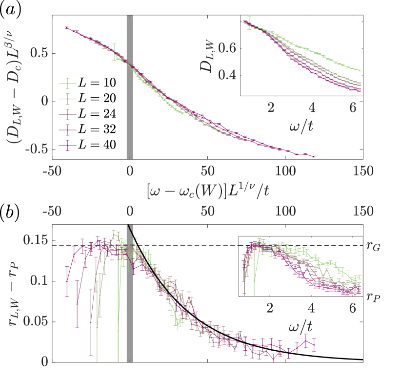
Next, we determine two independent estimates of for other at fixed and up to , which is necessary to determine the low energy ME at strong disorder. We take the crossing points of (i) -data with the finite-size critical dimension [Fig. 2, black arrow], as well as of (ii) exponential fits to -data with the critical gap ratio [see black line in Fig. 3 and Fig. 2, black arrow] 666Most of the time the exponential gap ratio fits slightly overestimate the critical energy, but always well within the errorbars.. For , respectively, Figs. 2 show the MEs [empty symbols, panels ] and binned -data [6 values per bin, panels ] close to the critical . We note that for in panels is neccessary to resolve the low energy ME as we discuss in the Supp. Mat. Excitingly, this procedure leads to consistent values for for all considered values of and . Interestingly, we find that for all data sets and sufficiently small , the dependence of on is consistent with the empirical ansatz
| (11) |
except for small where the gap to the upper band already vanishes at small . Corresponding exponential fits to the data, shown as thick black lines in Figs. 2(-), work well in a large part of the spectrum, while additional data obtained by increasing and matches up perfectly for disorder values beyond the truncation limit Note (4). Panel of Fig. 1 summarizes these findings, showing the extension of delocalized QP states up to the ME as a function of interaction at fixed energy with its greatest extension at , while the parameters of (11) are given in the inset of Fig. 1 depicting amplitudes and decay constants as functions of . We note that the perfect match of (11) for increased truncation and system sizes implies the absence of a thermal to fully QP localized phase, if extended to the thermodynamic limit De Roeck et al. (2016); Agarwal et al. (2017); De Roeck and Huveneers (2017).
V Trapped system
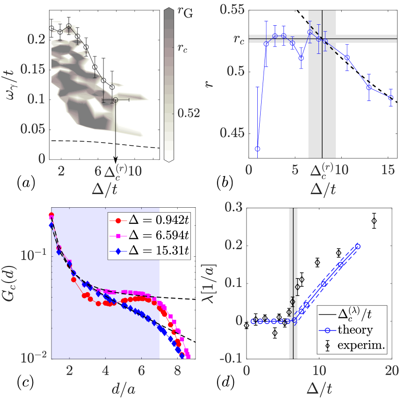
We end our discussion with the analysis of the added effect of a harmonic trap as realized in Choi et al. (2016) approximating the skewed Gaussian disorder used therein by an exact Gaussian with the full width at half maximum . All other parameters of (1) are taken from the reference so , the total particle number is 133 and we set with . In Fig. 4 we show the gap ratio of the QP spectrum related to a mean-field ground state with a central density of one surrounded by a condensate ring, contrary to the experiment which used a purely Mott-type initial state. The considered QP states localize at roughly the same energy scale as in the experiment, which we quantify by an exponential fit of for the least localized states at [see Fig. 4] resulting in a finite-size transition at 777Extremely small values of at small and in Fig. 12 result from nearly degenerate low energy pairs due to an approximate discrete rotational symmetry..
To get further insight we consider the scaling of connected single particle correlations as given by Here is the QP ground state expectation value implicitly defined via for all Bissbort et al. (2014); Geißler et al. (2018), thus best fulfilling the original approximation of neglected QP interactions [now added above]. We then consider the radial correlations of the four central sites averaged for each unique distance from the trap center [see Fig. 4]. Due to the vicinity to a localization transition and the inhomogeneous nature of the system we expect an interplay of algebraic and exponential correlations which we summarize in the fit function Note (4)
| (12) |
In Fig. 4 we show the various obtained inverse localization lengths of these fits together with one standard deviation of the fitting error. Below a certain disorder strength we find no exponential contribution. A linear fit for all nonzero yields the theoretical critical disorder strength comparing well to the experimental value , which, to our knowledge, is the first theoretical prediction. The different slope compared to experiment likely stems from the slightly different nature of the considered observables.
We note that the localization happens at a much smaller disorder strength than predicted for the unconfined system. This is most likely due to the trap enhanced variance of the local potential.
VI Conclusion
In conclusion, we have performed a detailed analysis of the two dimensional BHM with Gaussian disorder at half filling by discussing gap ratios and fractal dimensions of generalized (beyond Bogoliubov) QP eigenstates. We find a strongly localized spectrum with at least one mobility edge separating a small fraction of delocalized non-interacting QP modes at low energies from high lying localized ones. For all converged results this critical line follows an exponential decay with disorder down to quasiparticle energies of order . Finite-size scaling in the vicinity of these critical lines yields relevant critical exponents and parameters for a spectral transition characterized by a thermal-like gap ratio and weak multi-fractality. Furthermore, the MEs are strongly affected by the structure of QP bands in the clean system. Our method predicts a scaling of correlations almost identical to that observed in experiment Choi et al. (2016) and the finite-size transition point without requiring any empirical fit parameter.
As we show in this work, the FOE is a very promising tool for the analysis of extended systems with strong correlations, which can also be used to clarify the interplay between MBL and the BG Geißler (2020). As the FOE can easily be extended to the time domain, it furthermore opens up an exciting direction of future research into disorder-driven dynamical effects.
Acknowledgements.
A.G. would like to thank A. R. Abadal, C. Groß, L. Rademaker and J. Schachenmayer for insightful discussions. Support by the Leopoldina Fellowship Programme of the German National Academy of Sciences Leopoldina grant no. LPDS 2018-14, the ANR ERA-NET QuantERA - Projet RouTe (ANR-18-QUAN-0005-01) and the High Performance Computing center of the University of Strasbourg, providing access to computing resources and scientific support, is gratefully acknowledged. Part of the computing resources were funded by the Equipex Equip@Meso project (Programme Investissements d’Avenir) and the CPER Alsacalcul/Big Data. G.P. is further supported by USIAS in Strasbourg and the Institut Universitaire de France (IUF).References
- Anderson (1958) P. W. Anderson, Physical Review 109, 1492 (1958).
- Abrahams et al. (1979) E. Abrahams, P. W. Anderson, D. C. Licciardello, and T. V. Ramakrishnan, Physical Review Letters 42, 673 (1979).
- Fleishman and Anderson (1980) L. Fleishman and P. W. Anderson, Physical Review B 21, 2366 (1980).
- Roati et al. (2008) G. Roati, C. D’Errico, L. Fallani, M. Fattori, C. Fort, M. Zaccanti, G. Modugno, M. Modugno, and M. Inguscio, Nature 453, 895 (2008).
- Altshuler et al. (1997) B. L. Altshuler, Y. Gefen, A. Kamenev, and L. S. Levitov, Physical Review Letters 78, 2803 (1997).
- Basko et al. (2006) D. Basko, I. Aleiner, and B. Altshuler, Annals of Physics 321, 1126 (2006).
- Oganesyan and Huse (2007) V. Oganesyan and D. A. Huse, Physical Review B 75, 155111 (2007).
- Pal and Huse (2010) A. Pal and D. A. Huse, Physical Review B 82, 174411 (2010).
- Serbyn et al. (2013) M. Serbyn, Z. Papić, and D. A. Abanin, Physical Review Letters 111, 127201 (2013).
- Huse et al. (2014) D. A. Huse, R. Nandkishore, and V. Oganesyan, Physical Review B 90, 174202 (2014).
- Chandran et al. (2015) A. Chandran, I. H. Kim, G. Vidal, and D. A. Abanin, Physical Review B 91, 085425 (2015).
- Ros et al. (2015) V. Ros, M. Müller, and A. Scardicchio, Nuclear Physics B 891, 420 (2015).
- Imbrie et al. (2017) J. Z. Imbrie, V. Ros, and A. Scardicchio, Annalen der Physik 529, 1600278 (2017).
- Sierant and Zakrzewski (2018) P. Sierant and J. Zakrzewski, New Journal of Physics 20, 043032 (2018).
- Wahl et al. (2019) T. B. Wahl, A. Pal, and S. H. Simon, Nature Physics 15, 164 (2019).
- Imbrie (2016a) J. Z. Imbrie, Journal of Statistical Physics 163, 998 (2016a).
- Imbrie (2016b) J. Z. Imbrie, Physical Review Letters 117, 027201 (2016b).
- Nandkishore (2014) R. Nandkishore, Physical Review B 90, 184204 (2014).
- Kshetrimayum et al. (2019) A. Kshetrimayum, M. Goihl, and J. Eisert, (2019), arXiv:1910.11359 .
- Šuntajs et al. (2019) J. Šuntajs, J. Bonča, T. Prosen, and L. Vidmar, (2019), arXiv:1905.06345 .
- De Roeck et al. (2016) W. De Roeck, F. Huveneers, M. Müller, and M. Schiulaz, Physical Review B 93, 014203 (2016).
- Agarwal et al. (2017) K. Agarwal, E. Altman, E. Demler, S. Gopalakrishnan, D. A. Huse, and M. Knap, Annalen der Physik 529, 1600326 (2017).
- De Roeck and Huveneers (2017) W. De Roeck and F. Huveneers, Physical Review B 95, 155129 (2017).
- Lukin et al. (2019) A. Lukin, M. Rispoli, R. Schittko, M. E. Tai, A. M. Kaufman, S. Choi, V. Khemani, J. Léonard, and M. Greiner, Science (New York, N.Y.) 364, 256 (2019).
- Rispoli et al. (2019) M. Rispoli, A. Lukin, R. Schittko, S. Kim, M. E. Tai, J. Léonard, and M. Greiner, Nature 573, 385 (2019).
- Choi et al. (2016) J.-y. Choi, S. Hild, J. Zeiher, P. Schauß, A. Rubio-Abadal, T. Yefsah, V. Khemani, D. A. Huse, I. Bloch, and C. Gross, Science (New York, N.Y.) 352, 1547 (2016).
- Rubio-Abadal et al. (2019) A. Rubio-Abadal, J. Y. Choi, J. Zeiher, S. Hollerith, J. Rui, I. Bloch, and C. Gross, Physical Review X 9, 041014 (2019).
- Fallani et al. (2007) L. Fallani, J. E. Lye, V. Guarrera, C. Fort, and M. Inguscio, Physical Review Letters 98, 130404 (2007).
- Meldgin et al. (2016) C. Meldgin, U. Ray, P. Russ, D. Chen, D. M. Ceperley, and B. DeMarco, Nature Physics 12, 646 (2016).
- Fisher et al. (1989) M. P. A. Fisher, P. B. Weichman, G. Grinstein, and D. S. Fisher, Physical Review B 40, 546 (1989).
- Makivić et al. (1993) M. Makivić, N. Trivedi, and S. Ullah, Physical Review Letters 71, 2307 (1993).
- Zhang et al. (1995) S. Zhang, N. Kawashima, J. Carlson, and J. E. Gubernatis, Physical Review Letters 74, 1500 (1995).
- Priyadarshee et al. (2006) A. Priyadarshee, S. Chandrasekharan, J.-W. Lee, and H. U. Baranger, Physical Review Letters 97, 115703 (2006).
- Söyler et al. (2011) Ş. G. Söyler, M. Kiselev, N. V. Prokof’ev, and B. V. Svistunov, Physical Review Letters 107, 185301 (2011).
- Álvarez Zúñiga and Laflorencie (2013) J. P. Álvarez Zúñiga and N. Laflorencie, Physical Review Letters 111, 160403 (2013).
- Saliba et al. (2014) J. Saliba, P. Lugan, and V. Savona, Physical Review A 90, 031603(R) (2014).
- Álvarez Zúñiga et al. (2015) J. P. Álvarez Zúñiga, D. J. Luitz, G. Lemarié, and N. Laflorencie, Physical Review Letters 114, 155301 (2015).
- Bissbort et al. (2014) U. Bissbort, M. Buchhold, and W. Hofstetter, (2014), arXiv:1401.4466 .
- Geißler et al. (2018) A. Geißler, U. Bissbort, and W. Hofstetter, Physical Review A 98, 063635 (2018).
- Note (1) A crucial difference compared to the commonly considered box disorder is the presence of rare extreme peaks or wells in the potential.
- Note (2) We refer the interested reader to our follow-up work Geißler (2020) for a detailed discussion of the FOE method in the context of disordered systems.
- Note (3) We note that the MF self-consistency condition guarantees the absence of first order terms.
- Huber et al. (2007) S. D. Huber, E. Altman, H. P. Büchler, and G. Blatter, Physical Review B 75, 085106 (2007).
- Huber et al. (2008) S. D. Huber, B. Theiler, E. Altman, and G. Blatter, Physical Review Letters 100, 050404 (2008).
- Bissbort et al. (2011) U. Bissbort, S. Götze, Y. Li, J. Heinze, J. S. Krauser, M. Weinberg, C. Becker, K. Sengstock, and W. Hofstetter, Physical Review Letters 106, 205303 (2011).
- Endres et al. (2012) M. Endres, T. Fukuhara, D. Pekker, M. Cheneau, P. Schau, C. Gross, E. Demler, S. Kuhr, and I. Bloch, Nature 487, 454 (2012).
- Bogolyubov (1947) N. Bogolyubov, J.Phys.(USSR) 11, 23 (1947).
- Note (4) See Supplemental Material at [] for a discussion of details of the finite-size scaling analysis for the excitations and the ground state, a comparison of scenarios for the decay of correlations in a trapped system and a discussion of the entanglement captured by the FOE method.
- Gaul et al. (2015) C. Gaul, P. Lugan, and C. A. Müller, Annalen der Physik 527, 531 (2015).
- Atas et al. (2013) Y. Y. Atas, E. Bogomolny, O. Giraud, and G. Roux, Physical Review Letters 110, 084101 (2013).
- Hentschel and Procaccia (1983) H. Hentschel and I. Procaccia, Physica D: Nonlinear Phenomena 8, 435 (1983).
- Macé et al. (2019) N. Macé, F. Alet, and N. Laflorencie, Physical Review Letters 123, 180601 (2019).
- Lindinger et al. (2019) J. Lindinger, A. Buchleitner, and A. Rodríguez, Physical Review Letters 122, 106603 (2019).
- Note (5) From here on we omit the indices of the observables unless they are necessary.
- Note (6) Most of the time the exponential gap ratio fits slightly overestimate the critical energy, but always well within the errorbars.
- Note (7) Extremely small values of at small and in Fig. 12 result from nearly degenerate low energy pairs due to an approximate discrete rotational symmetry.
- Geißler (2020) A. Geißler, (2020), arXiv:2011.10104 .
- Bissbort (2012) U. Bissbort, Dynamical effects and disorder in ultracold bosonic matter, Ph.D. thesis, Johann Wolfgang Goethe-Universität (2012).
- Geißler (2018) A. Geißler, Lattice-supersolids in bosonic quantum gases with Rydberg excitations, Ph.D. thesis, Johann Wolfgang Goethe-Universität (2018).
- Harris (1974) A. B. Harris, Journal of Physics C: Solid State Physics 7, 1671 (1974).
- Chayes et al. (1986) J. T. Chayes, L. Chayes, D. S. Fisher, and T. Spencer, Physical Review Letters 57, 2999 (1986).
- Vojta and Hoyos (2014) T. Vojta and J. A. Hoyos, Physical Review Letters 112, 075702 (2014).
- Jensen (1999) I. Jensen, Journal of Physics A: Mathematical and General 32, 5233 (1999).
- Wang et al. (2013) J. Wang, Z. Zhou, Q. Liu, T. M. Garoni, and Y. Deng, Physical Review E 88, 042102 (2013).
- Fisher and Fisher (1988) D. S. Fisher and M. P. A. Fisher, Physical Review Letters 61, 1847 (1988).
- Herbut (1997) I. F. Herbut, Physical Review Letters 79, 3502 (1997).
- Tikhonov and Mirlin (2019) K. S. Tikhonov and A. D. Mirlin, Physical Review B 99, 024202 (2019).
- Note (8) While, in principle, this argument can be repeated for any number of non-interacting FOE quasiparticle excitations, previously neglected interaction terms become increasingly relevant.
- Frérot and Roscilde (2015) I. Frérot and T. Roscilde, Physical Review B - Condensed Matter and Materials Physics 92, 115129 (2015).
- Frérot and Roscilde (2016) I. Frérot and T. Roscilde, Physical Review Letters 116, 190401 (2016).
Supplemental Material for
“Mobility edge of the two dimensional Bose-Hubbard model”
The numerical results presented in the main text are the result of an extensive finite-size scaling analysis of the quasiparticle (QP) spectrum for a disordered Bose-Hubbard model obtained using the fluctuation operator expansion method Bissbort (2012); Bissbort et al. (2014); Geißler (2018); Geißler et al. (2018). In the main text we also discuss the scaling of single particle correlations in an experimentally relevant system with harmonic confinement. Here, we provide further details on the finite-size scaling procedure and fitting of the correlations in the trapped system. In Sec. I we give an in-depth discussion of the procedure to obtain the finite-size scaling collapse of the level spacing ratios and the fractal dimensions of the quasiparticle wave functions in terms of the mean relative variances as a measure for the goodness of the collapse. We also comment on the limits of our numerical calculations due to the necessity of a basis truncation. Subsequently, in Sec. II we use a very similar measure to quantify the presence of a structural ground state phase transition in the inhomogeneous mean-field ground state, which the FOE is based upon, consistent with earlier predictions for a zero-energy superfluid to Bose-glass transition Fisher et al. (1989); Makivić et al. (1993); Zhang et al. (1995); Priyadarshee et al. (2006); Álvarez Zúñiga et al. (2015). We furthermore discuss possible scenarios for the decay of correlations of the QP ground state of the disordered Bose-Hubbard model in a harmonic trap in Sec. III, which we relate to experimental results in the main text. Finally, in Sec. IV we point out the occurrence of many-body entanglement in the FOE, as its presence is highly relevant to the physics of many-body localization.
I Finite-size scaling at the Mobility Edge (ME)
First, we give a systematic finite-size scaling analysis of the quasiparticle (QP) spectra revealing the mobility edge in the QP fluctuations at given and . For the two considered observables we obtain mutually consistent scaling exponents, which are also consistent with the Harris criterion Harris (1974); Chayes et al. (1986); Vojta and Hoyos (2014) implying that the critical point is not destabilized by Griffiths singularities. In general, second order phase transitions can be characterized by a generic algebraic scaling, which, for the two considered observables gap ratio and fractal dimension in the vicinity of the mobility edge, takes the form
| (S13) | ||||
| (S14) |
Here, and are the scaling functions, the index signifying a weak dependence on the disorder, while is the rescaled length scale. The universal scaling exponents and are to be determined numerically in combination with the ME critical energies and the critical fractal dimension . In the following we give a detailed discussion of the finite-size scaling collapse, which is performed at , and for with corresponding numbers of realizations . The range of QP energies and disorder strengths is chosen such as to cover as much as possible of the low energy ME between the lowest finite-size resolvable modes and the first band edge. We perform a binning for each and data set given by 30 equally spaced energies in the given interval. Each bin contains disorder averaged data points closest in mean QP energy to each energy , with dependent on system size (chosen such that on average there is a slight overlap between the bins).
I.1 Scaling analysis for the gap ratio
For the gap ratio the scaling ansatz (S13) involves a single scaling exponent in addition to the critical energies . In order to find the latter we note that as a function of the QP energy at given and for any system size always starts to decay from the thermal value at a common QP energy. The tails of this decay almost exactly follow an exponential, as visible in plots of the unscaled data [see main text and insets in Fig. S1()]. Such a behavior is consistent with a phase transition which in this case we expect to be a transition from delocalized to localized states in the QP spectrum. Thus the universality of phase transitions implies that exponential fits to the mentioned tails should cross in a single point at a certain QP energy, the critical energy corresponding to the ME. Thus we can obtain a remarkably good estimate of for all considering the noise of the sampled data. Still, we also use differences in the decay constants of these exponential fits as weights in the averaging over the crossing points so the mean is not affected by large outliers due to nearby system sizes having very similar decay constants in their exponential fits (see for example inset Fig. S1(, right)).
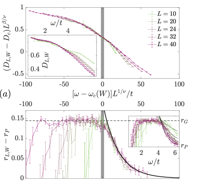
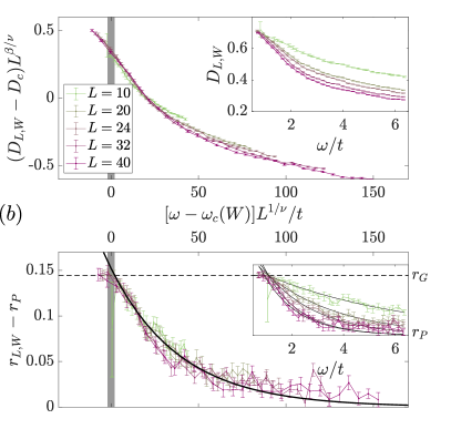
Next we define a model independent measure for the goodness of the remaining single parameter scaling collapse involving only the parameter . For this purpose it is beneficial to define the rescaled energies
| (S15) |
where the indices and are used to identify the individual binned data sets at all corresponding energies . From these we define the interpolated functions . Then, the best choice of the scaling exponent minimizes the following mean relative variances,
| (S16) |
where are the standard errors of the mean determined from the binned data, while the normalization constants are given by the total sum of all inverse relative covariances, used as weights to account for the noise,
| (S17) |
Ideally, if all data points collapse onto the unknown scaling function within their error bars, this measure should be of order 1 or less. Note that we only consider due the systematic finite-size effects resulting from symmetry related level bunching for low energy QP modes which are near plane wave excitations at weak disorder. Otherwise, we find that the finite-size scaling barely affects the delocalized states as implying a near-thermal critical behavior.
Due to the observed weak dependence of the scaling function on , visible in the much slower decay of the collapsed data in Fig. S1 at large disorder, each disorder value is treated independently in the collapse of the binned gap ratio data quantified by (S16). To approximate the error of the scaling collapse we sample over the results for all which we write as . For the mean relative variances and its standard deviation we find . Regarding the universal exponent, the described minimization results in . Sampling all collapsed data sets in the vicinity [marked by the vertical dark gray regions in Figs. S1()], chosen such that the value and its standard deviation are converged, further yields the critical gap ratio with the average over considered disorder values and system sizes .
I.2 Scaling analysis for the fractal dimension (q=2)
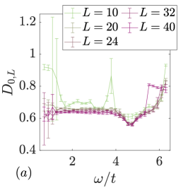
Finding the proper finite-size scaling of the fractal dimension is much harder compared to the gap ratio as Eq. (S14) has twice the number of scaling exponents and parameters at any given disorder . To find a unique prediction we determine the parameters step by step via independent means. Firstly, we note that for fixed QP energies and as a function of disorder the fractal dimension always has a sigmoid shape. At the same time finite-size scaling tells us that the inflection points of such a series of sigmoid functions have to collapse onto a single point of the scaling function. Correspondingly, for any of these fixed QP energies , where is the scaled disorder, in analogy to Eq. (S14) one also gets
| (S18) |
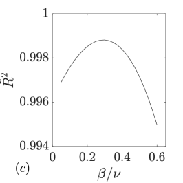
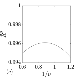
As we know the fractal dimension only for a limited set of disorder values we use a fit to a generic sigmoid function [] to determine the inflection points and thus as a function of . A few examples of such fits are shown in the insets of Figs. S7(). In order to obtain a sufficiently good estimate of an inflection point it cannot be too close to the edges of the data range or even outside. We find the most consistent estimates to be in the range of energies (see Fig. S2()). As all within this range are consistent with each other we can take an average over these QP energies. The resulting values we then fit by Eq. (S18) where we consider as an unknown parameter, such that this fit is slightly over-determined. Thus we take as a fixed parameter of these fits to obtain sets of best and as functions of . We find a wide range of between 0.1 and 0.5 giving very similar quality of fits [compare Fig. S2()], as quantified by the adjusted coefficient of determination shown in Figs. S2().
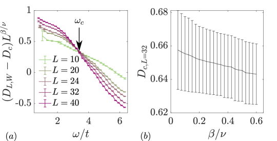
In a next step we determine the critical QP energies from the mutual crossing points of the scaled fractal dimension as a function of QP energies for fixed disorder values, using from the previous step. Figure S3() shows and example using with . The collection of all these crossing points yields the ME as well as the finite-size critical dimension . Prior knowledge of the scaling function could also be used to determine the critical ME for any single finite-size system without having to perform a full finite-size collapse. But as the scaling function has a weak disorder dependence, also varies slightly along the ME. As the scaling function is non-universal, we approximate the error of the disorder averaged finite-size critical dimension , for , by its standard deviation to account for these variations. As shown in Fig. S3() for the finite-size critical dimension and thus also the predicted ME barely depends on the scaling exponent within the optimal region [see Fig. S2()].
Finally, keeping all parameters including the ME at all considered disorder values except fixed, we perform the final collapse by minimizing the following mean relative variances
| (S19) |
where are the standard errors of the mean determined from the binned data, while the normalization constant is given by the total number of terms, . As stated before, for an ideal collapse such a measure should be of order one.
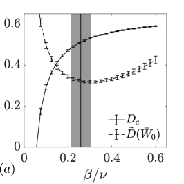
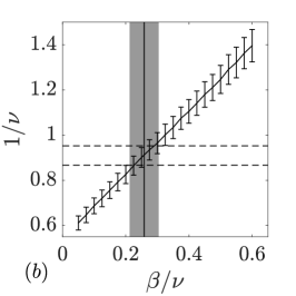
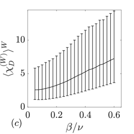
Now, the minimization of Eq. (S19) is performed for each considered disorder value and for various . Each comes with a ME and critical dimension [see Fig. S4()]. Averaging the resulting best over the considered disorder data sets reveals a nearly linear relation between and of the best collapses. Requiring that has to be identical to the value obtained for the collapse of the gap ratio data in the preceding section () yields the prediction for the scaling exponent , as shown in Fig. S4(). We note that these scaling exponents are consistent with those of the one-dimensional directed percolation universality class Jensen (1999); Wang et al. (2013). Due to some rare systematic finite-size effects for small system sizes and weak disorder (compare finite-size prediction of the mobility edge for shown in Fig. S8), we quantify the quality of these best collapses by considering the typical value of Eq. (S19), which we obtain using the definition and its standard deviation, see Fig. S4(). As a result of some finite-size corrections, especially for the smallest system sizes (compare examples in Fig. S1 and finite-size prediction of the ME in Fig. S8), this measure is slightly larger then one due to some large deviations of the full finite-size collapse appearing far from the critical point [note especially the very small errors in the fractal dimension at very low QP energies in Fig. S1()].
I.3 Further scaling observations and remarks
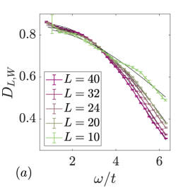
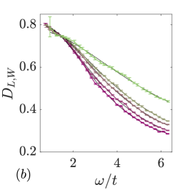
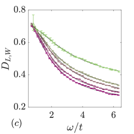
The idea to follow the finite-size scaling of special points of the scaling function can also be applied to the fractal dimension of the QP states as a function of energy for fixed disorder and various system sizes . But in this case the previously used ansatz of using a -shaped function to determine the inflection points does not work due to the strong asymmetry of . Instead, motivated by the empirically obtained shape of the ME , we instead consider the fit function
| (S20) |
Via this fit we find the approximate inflection points . Similar to before, this procedure works best when the QP energy of the inflection point is sufficiently far from the considered energy limits, so for . Furthermore, at weak disorder and low QP energies we find some deviation from the empirical fit function (compare Figs. S5). In Figs. S6 we show the scaling behavior of and . Very clearly these data points imply for , or more precisely for with the error given by the standard deviation. This is consistent with the value of the critical fractal dimension determined in the finite-size scaling above. Only for , where we expect the fit to be less reliable, do we observe apparent finite-size scaling behavior, but with relatively large uncertainties for the inflection points. On the other hand shows very consistent scaling behavior, such that we can attempt a scaling collapse similar to Eq.(S18):
| (S21) |
As is the mobility edge and as such not a constant, we combine the data sets for where we consider the inflection points to be most reliable. Via this sampling we reduce the noise in the combined data so we are best able to determine the optimal scaling exponent by fitting to the average of Eq.(S21) over the disorder for various values of and considering the adjusted coefficient of determination shown in Fig. S6. While we find a wide range of parameters that give very similar values of the optimum is at about consistent with our earlier finding. In Fig. S6 we also show fits of Eq. (S18) with which all fit the inflection point data within the respective errorbars.
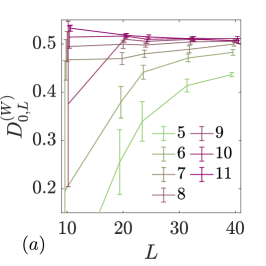
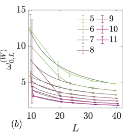
As we have seen, the scaling parameters are consistent both for a finite-size scaling along the QP energies and fixed disorder, as well as for variable disorder and fixed QP energies. Therefore, for the sake of completeness we also show exemplary full collapses at fixed QP energies using with as the binning centers. The resulting scaling collapses are shown in Fig. S7 for the scaling exponents and parameters determined earlier. Indeed, these parameters result in remarkably good collapses for the different parts of the spectrum.

Finally, in the main text we also show the finite-size scaling prediction of the ME in the thermodynamic limit by considering the finite-size critical contour where is the critical fractal dimension and is the value of the scaling function at the critical point. As can be seen in Fig. S8, all finite size predictions of the ME match almost exactly except for some deviations for small system sizes. We note that the reentrant shape of the contour lines at strong disorder and low energies is a truncation artifact as we will discuss now.
We note that, especially at large energies as well as the low excitation energies relevant here, another scaling in addition to becomes important as well. This is related to the Bose statistics, namely its unbounded local Fock-bases of bosonic number states, which in numerical simulations is commonly truncated at some sufficiently large number . Within the FOE method this truncation is realized on the level of considered mean-field Gutzwiller (eigen-)states at each site, . We always use to get a good approximation of the low energy part of the considered local operators in terms of the MF states. Furthermore, in the main part we consider the up to lowest MF states at each site which is sufficient to resolve the ME down to , while for the energy and disorder window considered for the finite-size scaling (see main text and Sec. I.1 and I.2) already is sufficient, as we will see in a moment. Only as the ME approaches the lowest resolved QP energy levels – those following an unphysical reentrant shape (see Fig. S8) – do we observe a pronounced dependence of the numerical results for the (multi-)fractal dimension of the QP states on the truncation , as we show in Figs. S8() for weak and strong interaction , respectively. Comparing with one can see that in terms of the QP states are well converged at all QP energies down to those QP levels for which has its unphysical maximum at . In Fig. S8 the dotted line represents the energy of this maximum as an approximate bound below which the QP states can not be considered converged in terms of the considered local basis truncation .
II Characterization of the mean-field ground state phase transition
It has long been established that the ground state of a disordered two-dimensional Bose-Hubbard model, as used in the main part, can exhibit the formation of a so-called Bose-glass phase Fisher and Fisher (1988); Fisher et al. (1989); Herbut (1997); Söyler et al. (2011); Álvarez Zúñiga et al. (2015). In this section we briefly comment on the relation of our results to these earlier predictions on the level of the fragmentation of the mean-field ground state. As we will show, such a transition for finite values of can be also determined by an in-homogeneous mean-field description which at the same time forms the basis of the FOE method used in the main text and above. Our results are consistent with a direct phase transition from a condensed superfluid to a Bose-glass in the ground state. For example, earlier works using a uniform disorder distribution (best compared to the full width at half maximum of a Gaussian distribution with standard deviation ) have predicted this transition to be at Fisher et al. (1989); Makivić et al. (1993); Zhang et al. (1995); Priyadarshee et al. (2006); Álvarez Zúñiga et al. (2015) at half-filling and in the limit of infinite interaction , the so-called hard-core boson case.
To characterize the phase transition in the ground state of the disordered Bose-Hubbard model in two dimensions we consider the limit of the multi-fractal dimensions as an order parameter. Applied to the distribution of the inhomogeneous mean-field condensate order parameter and sampled over the disorder realizations we define
| (S22) |
As in the main part we evaluate this observable over a range of disorder strengths , fixed interaction and for the same linear system sizes while averaging over disorder realizations each time.

In Fig. S9() we show and its difference quotient revealing an inflection point in the function , which experiences a finite-size scaling shift. We obtain via parabola-fits to the minima in the difference quotient. Analogous to the mobility edge we consider a scaling ansatz of the form
| (S23) |
For the scaling collapse of the inflection points onto the inflection point of the scaling function , where is the rescaled disorder, we thus expect
| (S24) |
As this expression has three unknown parameters compared to the 5 considered system sizes we first determine the best fit parameters and for various values of . An exemplary fit for is shown in Fig. S9(). As the finite-size scaling at the critical point is independent of the scaling exponent , we can further determine from the crossing points of the data sets for various system sizes if we only apply the scaling to the fractal dimension as shown in the inset of Fig. S9(). This way we get the best candidates for the critical point as a function of depicted in Fig. S9(). To quantify the goodness of these fits we consider the adjusted coefficient of determination given in the inset of Fig. S9(). For the considered range of is almost constantly at its optimum but as the fractal dimension by definition is limited to we find a fixed lower bound for [see Fig. S9()].
For the final collapse we only have to consider and in order to minimize the mean relative variance as a measure for the goodness of the collapse:
| (S25) |
Analogous to the finite-size scaling at the mobility edge, are the standard errors of the mean determined from the disorder sampling while the normalization constant is given by the total number of terms, . In order to estimate the error of the obtained scaling exponents, this finite-size scaling procedure is repeated for 6 independent subsets of 10 disorder realizations each. For the best collapses we find corresponding to the mean-field scaling exponents and while the critical point has at a disorder of . We thus find a ground state transition point at that is consistent with previous predictions of a superfluid to Bose-glass transition also at half-filling but in the limit and for equal distributed box-disorder of the local potential Makivić et al. (1993); Zhang et al. (1995); Priyadarshee et al. (2006); Álvarez Zúñiga et al. (2015).
III Single particle correlations in a trap
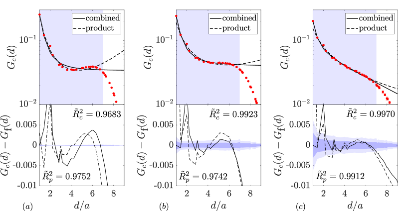
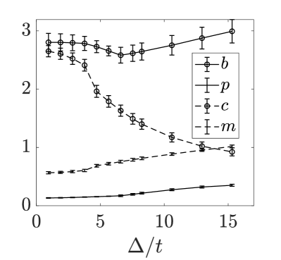
As in the experiment we consider a finite-size system in a harmonic trap Choi et al. (2016), thus particles with a phase coherence over only a finite length scale, driven by the competition of repulsive Hubbard interactions and local disorder, may still span the whole system, forming a local BEC in the ground state. Only for vanishing disorder and interaction do all particles participate in the condensate mode, while a finite condensate order parameter is observed in the ground state even as both interaction and disorder are increased (with the typical wedding cake structure in the homogeneous case). For finite-size systems at the superfluid to Bose-glass transition the condensate order parameter also does not vanish at the critical point and beyond Meldgin et al. (2016). In this confined system, it is thus reasonable to assume a crossover in the ground state where a fraction of the particles always exhibits long-range correlations with a short-distance algebraic decay, as in a condensate, and only the remaining fraction can be localized more strongly. So, as a first scenario for , where the distance is in units of the lattice spacing , we assume the empirical linear combination form
| (S26) |
We fix the amplitude of this ansatz by the value for nearest neighbors. Then corresponds to the relative contribution of the exponential decay with the decay constant and the algebraic decay with the exponent . We consider the latter three as fit parameters.
On the other hand, related work on Anderson localization on random regular graphs, where every site has nearest neighbors, suggests a product of exponential and algebraic decays instead Tikhonov and Mirlin (2019),
| (S27) |
Due to the similarity of the effective quasiparticle Hamiltonian to such systems it might be considered a possible model theory for the non-interacting quasiparticles, with the effective number of nearest neighbors and the algebraic decay constant. Together with the amplitude we thus have three fit parameters, as well.
In Fig. S10 we show exemplary best fits of these two scenarios to our numerical data for various values of the disorder . In most cases the adjusted coefficient of determination for the product scenario is slightly worse compared to the linear combination form. Furthermore, only for strong disorder does the product form not diverge as . Except for the decay constant of the exponential term in the linear combination form discussed in the main part, we show all the relevant parameters in Fig.S11. Here we can see that the apparent unphysical behavior of the product form Eq. (S27) stems from . For the linear combination form Eq. (S26), on the other hand, the exponent of the algebraic term remains constant within its errorbars, as one would expect for the assumed two components. Finally, the relative contribution of the localized component starts to increase precisely at the transition.
IV Entanglement
In the following we show that the Fluctuation operator expansion (FOE), while based on a mean-field representation, is able to capture effects of many-body entanglement in strongly correlated systems. To do so we first present a qualitative argument for the occurrence of non-trivial entanglement in this method and then discuss some numerical examples for the disordered Bose-Hubbard model central to this work.
A typical measure of entanglement is the von Neumann entanglement entropy evaluated for the density operator of any subsystem . For a closed system (with ) one has . In order for to be non-zero, which signifies entanglement, the Schmidt rank counting the non-zero eigenvalues of has to be greater than one. We will now show this property for typical FOE states. To perform the partial trace using the FOE method we consider and an analogous form for any QP added state . At first glance this ansatz seems to necessitate explicit knowledge of the state. In contrast, it is straightforward to consider the Gutzwiller bases to gain some insight into the structure of . Each of its matrix elements
| (S28) |
is given by the correlations of local QP ground state excitations. The properties of and guarantee that only correlations of even order in the Gutzwiller operators are non-vanishing. Thus, is separable into two sectors, one consisting of even numbers and one consisting of odd numbers of local excitations as correlations coupling these sectors are of odd order in the Gutzwiller operators and thus vanish.
As represents a correction of the MF ground state, the relevant sector of has to contain the MF state and is the even sector. Now we consider an arbitrary bipartition ( and ) of a system consisting of at least two sites. Except for the trivial case , coefficients then fall into two mutually distinct groups. Either, the corresponding basis vectors in the subspaces of and are both in the odd sector, or, they are both in the even sector. Thus there are always non-trivial submatrices of where all involved eigenvector pairs of both subspaces and are mutually orthogonal. This implies that a Schmidt decomposition then yields a nontrivial Schmidt rank greater than one. Finally, as a single QP added state resides in the odd subspace of Gutzwiller excitations, one can apply the same argument with the only difference being that the paired subspaces of and are then always of opposite order. Therefore, we conclude that the FOE predicts nontrivial entanglement properties of a strongly correlated system for the ground state as well as its many-body excitations 888While, in principle, this argument can be repeated for any number of non-interacting FOE quasiparticle excitations, previously neglected interaction terms become increasingly relevant..

Let us now quantify the amount of entanglement beyond this qualitative argument. The quadratic form of the approximate FOE Hamiltonian implies the applicability of Wick’s theorem, as has been discussed for a closely related method Frérot and Roscilde (2015, 2016). Thus, assuming the Gutzwiller operators to be exactly bosonic (see main text), the reduced density matrix can be reconstructed from the two-point correlations only. The relevant correlations are and for which one can show the relation
| (S29) |
where is a Bogoliubov transformation and is the occupation of the th mode of a quadratic Hamiltonian fulfilling the identity . Thus the von Neumann entanglement entropy of can be obtained via
| (S30) |
This representation applies to any eigenstate of a quadratic Hamiltonian with anomalous hopping. Therefore, we can determine for the ground state as well as the excitations. For the ground state we consider the case and for a system with . We define the region as all sites within a radius of a given site where we have defined . We average of 60 positions for for each of the realizations we consider. Fig. S12 shows as a function of the disorder strength for the truncations and , as well as . One can see that is independent of the truncation up to indicating converged results for any disorder below this value. Furhtermore, the linear dependence of on ends with a kink at about . The position of this kink is close to the ground state phase transition discussed for the mean-field state in Sec. II. In addition, Fig. S12 shows that as a function of is mostly constant for various values of the disorder strength. This is consistent with the expectation of an area law for the entanglement growth typical for the ground state. Deviations from a constant at large and small can be attributed to finite size effects within our periodic system.
Next we consider a system of sites with periodic boundaries to analyze the entanglement in the QP excitations at and . To do so we define as strips of varying width wrapped along the short direction. is then sampled for realizations and over the 24 possible positions of the strip for each disorder realization, each time taking the excitation closest in energy to . As shown in Fig. S12 for a width of sites, is approximately constant up to a critical excitation energy beyond which it decreases continuously. The position of this kink is consistent with the near-thermal ME derived above (see Sec. I). Finally, by also considering as a function of the width we observe very different behavior in the ground state compared to the QP excitations (see Fig. S12). On the one hand the ground state entanglement can be fit nearly exactly by the ansatz
| (S31) |
suggesting a logarithmic correction to the area law in the ground state. Such a correction is expected in a superfluid ground state Frérot and Roscilde (2016) as the considered disorder strength is below the critical value. But, on the other hand panel shows that the best fits of the logarithmic ansatz for the excitations at (cross symbols) and (circular symbols) have substantial systematic deviations and a much lower compared to the ground state. The (finite-size) entanglement growth of the excitations is thus inconsistent with a logarithmic growth suggesting a faster growth of with the volume for fixed boundary area of the region . The observed relation is approximately consistent with a square-root behavior, although an accurate prediction would require a greater range of system sizes beyond the scope of this discussion.
In conclusion, as discussed qualitatively and quantitatively in this section, the FOE method is able to capture non-trivial entanglement both in the ground state and in its QP excitations. In the ground state it predicts the commonly expected area law behavior, while it even predicts faster then area law (possibly even volume law) entanglement growth for the (near-)thermal QP excitations in the vicinity of the ME.