Border effect corrections for diagonal line based recurrence quantification analysis measures

Abstract

Recurrence Quantification Analysis (RQA) defines a number of quantifiers, which base upon diagonal line structures in the recurrence plot (RP). Due to the finite size of an RP, these lines can be cut by the borders of the RP and, thus, bias the length distribution of diagonal lines and, consequently, the line based RQA measures. In this letter we investigate the impact of the mentioned border effects and of the thickening of diagonal lines in an RP (caused by tangential motion) on the estimation of the diagonal line length distribution, quantified by its entropy. Although a relation to the Lyapunov spectrum is theoretically expected, the mentioned entropy yields contradictory results in many studies. Here we summarize correction schemes for both, the border effects and the tangential motion and systematically compare them to methods from the literature. We show that these corrections lead to the expected behavior of the diagonal line length entropy, in particular meaning zero values in case of a regular motion and positive values for chaotic motion. Moreover, we test these methods under noisy conditions, in order to supply practical tools for applied statistical research.

In recurrence quantification analysis, border effects and tangential motion can heavily bias diagonal line based characteristics.

Border effect bias can be minimized by a simple alteration of the diagonal line length histogram.

A parameter free, skeletonization method reduces artifacts due to tangential motion and leaves a RP of thin diagonal lines.

The proposed correction schemes lead to diagonal line entropy values that fall within analytically derived expectation ranges, even in the presence of noise.

1 Introduction

Recurrence quantification analysis (RQA) is a powerful tool for the identification of characteristic dynamics and regime changes [1, 2]. This approach is successfully applied in many scientific disciplines [3, 4, 5, 6, 7, 8, 9, 10, 11, 12, 13]. Several measures of complexity are defined on geometric features (such as diagonal and vertical lines) in the recurrence plot (RP), which represents time points $j$ when a state $\vec{x}_{i}$ at time $i$ recurs [14, 3, 1, 2]. These line structures represent typical dynamical behavior and are related to certain properties of the dynamical system, e.g., chaotic or periodic dynamics. Therefore, their quantitative study by the RQA measures within sliding windows is a frequently used task for the detection of regime changes [15, 16, 17, 2]. However, as some RQA measures rely on the probability distribution of the lengths of the diagonal lines in an RP, the artificial alteration of these lines due to border effects [18, 17], insufficient embedding [1, 19], or a certain sampling setting [20, 21] can have significant impact on these measures. A few ideas have been suggested to overcome such problems [18, 22, 23]. Here we review these ideas, propose novel correction schemes, and systematically compare them.

2 Recurrence quantification analysis and border effects

A recurrence plot (RP) is a binary, square matrix $\mathbf{R}$ representing the recurrences of states $\vec{x}_{i}$ ($i=1,...,N$, with $N$ the number of measurement points) in the $d$-dimensional phase space [24, 1]

$${R}_{i,j}(\varepsilon)=\Theta\left(\varepsilon-\|\vec{x}_{i}-\vec{x}_{j}\|\right),\qquad\vec{x}\in\mathbb{R}^{d},$$ (1)

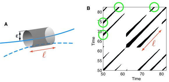
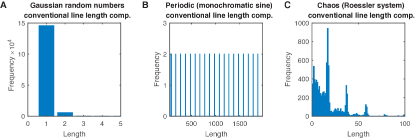
with $\|\cdot\|$ a norm, $\varepsilon$ a recurrence threshold, and $\Theta$ the Heaviside function. The RP consists of small-scale structures, such as single points and diagonal and vertical lines, which characterize important dynamical properties of the system. A diagonal line is a sequence of pairs of time points $\mathcal{L}\colonequals\{(i,j),(i+1,j+1),\ldots,(i+\ell-1,j+\ell-1)\}$ where ${R}_{i,j}\equiv 1$ for all index pairs in $\mathcal{L}$. Diagonal lines in the RP represent the temporal duration that two distinct parts of the phase space trajectory run parallel (Figs. 1 and 2). The histogram $P(\ell)$ of the lengths of diagonal lines (Fig. 3) characterizes the dynamics [25, 26, 27] and can be and has been used to quantitatively distinguish between RPs, the underlying dynamics, or to identify regime transitions [15, 3, 11, 12, 13].

For uncorrelated noise, the probability to find a line $\mathcal{L}$ of exact length $\ell$ decays exponentially [28] (Fig. 3A), i.e., the RP consists only of very short diagonal lines, if there are any lines at all (Fig. 2A). In contrast, for chaotic dynamics, the RP contains diagonal lines of different lengths (Fig. 2C), resulting in a broad distribution $P(\ell)$ (Fig. 3C). The RP for a periodic system contains continuous, non-interrupted diagonal lines, virtually of infinite length (Fig. 2B). In principal, we would expect a discrete line length distribution with a peak at line length infinity. However, the lines are cut at the begin and end of the RP, such that an uncorrected conventional line length measurement results in a discrete distribution $P(\ell)$ with uniform characteristics (Fig. 3B).

Figure 1: Parallel and close parts of a phase space trajectory (A) correspond to diagonal lines of length $\ell$ in an RP (B). Diagonal lines can be cut by the border of the RP (green circles).

The RP is a discrete matrix. Therefore, the creation of the histogram $P(\ell)$ appears to be trivial. But it is not as simple as it looks at the first glance. Diagonal lines can be quite long and – as already mentioned – can exceed the finite size of the RP. In practice, this is a very common problem, particularly when a sliding window method is applied. How to count such diagonal lines? As we will see later, for some measures, it can be important to have the correct length of the lines, for other measures it does not play any role. In the original definition, the lines are also counted even if they were cut by the RP border [14, 29, 1].

Several measures for RP analysis have been introduced which use $P(\ell)$. The firstly introduced measure was the determinism [29]. This measure is the fraction of recurrence points that form diagonal lines

$$D=\frac{\sum_{\ell=\ell_{\min}}^{N}P(\ell)}{\sum_{\ell=1}^{N}\ell P(\ell)}$$ (2)

and considers lines which have at least length $\ell_{\min}$, which in principle is a free parameter, but often set to 2. Nevertheless the choice of the minimal line length can be crucial for the correct estimation of some RQA measures and we come back to that in Sect. 6.1. More details about this can be found in [1]. Since RPs of uncorrelated noise have mainly single points and only few and short diagonal lines, for such dynamics $D$ has rather low values (although embedding can result in artificially high $D$ values, see discussion in [19, 30]). In contrast, RPs for deterministic dynamics contain of many diagonal lines, resulting in elevated values of $D$, with the special case of $D=1$ for periodic and quasi-periodic dynamics. As this measure only quantifies whether a recurrence point is on a diagonal line or not, the actual length of a diagonal line is not important (i.e., whether the line crosses the RP border or not).

Another idea is to look at the average and maximal length of the detected diagonal lines (related to prediction time and Lyapunov exponent, resp.[1]). The average, of course, depends on the actual line lengths and will be biased when diagonal lines cross the RP borders.

Because the shape of $P(\ell)$ differs for different dynamics, the Shannon entropy of the probability distribution $p(\ell)=\frac{P(\ell)}{\sum_{\ell}P(\ell)}$ to find a diagonal line of exact length $\ell$ was suggested [29]

$$S=-\sum_{\ell=\ell_{\min}}^{N}p(\ell)\ln p(\ell).$$ (3)

This measure was introduced in a pragmatic way to quantify the visual line structures in the RP and has been interpreted as the “information content of the trajectories” [31]. Here, the choice of the minimal line length $\ell_{\min}$ has a significant effect, since it discards parts of the line length histogram and therefore alters its shape. For uncorrelated noise, $S$ has low values, because $p(\ell)$ is exponentially decaying. For chaotic dynamics, $p(\ell)$ is a broad distribution, resulting in quite large $S$ values. However, for periodic signals $p(\ell)$ has more similarity with a uniform distribution if the mentioned border effects are not accounted for. Therefore, $S$ is not low for periodic signals, although we would expect it, but rather large, even larger than for chaotic dynamics. Here, the effect of the sliced lines at the RP border has the strongest and remarkable effect, which is why we focus on this measure only in this letter. Maximal and mean diagonal line length and specifically determinism and their behavior with respect to border effects, the choice of further RP related parameters and its interpretation will be examined carefully in a forthcoming paper.

Figure 2: RPs of (A) standard normal Gaussian numbers, (B) time-delay embedded sinusoidal with an oscillation period $T=100$ time units ($m=2$, $\tau=T/4$), and (C) the Rössler system ($a=0.15$, $b=0.2$, $c=10$) (only subsets shown). RPs were constructed from time series of 2,000 samples (in case of the Rössler system we removed transients) using a constant global recurrence rate of 4% with a fixed threshold and Euclidean norm.

Figure 3: Diagonal line length distributions of the different systems types described in Fig. 2, gained from the conventional line counting.

3 Correction schemes for counting diagonal lines

In this section we show two ways of overcoming the problem of biased diagonal line based measures due to the border effect. Either we manipulate the histogram of the diagonal lines (Sect. 3.1) or we change the shape of the RP in order to avoid a bias in the first place (Sect. 3.2).

3.1 Alternative ways of counting line lengths

Let R be a $N\times N$ recurrence matrix, Eq. (1), and $P(\ell)$ the histogram of the diagonal lines contained in R. We now substantiate the definition of a diagonal line in an RP from Sect. 2. A diagonal line $\mathcal{L}$ of length $\ell$ is a set of $\ell$ index tupels $(\cdot,\cdot)_{k=1,..,\ell}$:

$$\mathcal{L}_{\ell}\colonequals\{(i+k,j+k)\ |\forall k=0,...,\ell-1\ :\ \left(1-{R}_{i-1,j-1}\right)\left(1-{R}_{i+\ell,j+\ell}\right){R}_{i+k,j+k}\equiv 1\}.$$ (4)

The length of a line $\ell,$ is usually the cardinality of this set $|\mathcal{L}|$.

We denote any diagonal line which starts and ends at the border of R as a border diagonal, e.g., in case of the lower triangle of the RP, when starting at $(i,1)$ in the first column and ending at $(N,N-i+1)$ in the last row:

$$\mathcal{L}_{\text{border}}\colonequals \{(i+k,1+k)\ |\ \forall\,k=0,\ldots,N-i\ :\ {R}_{i+k,1+k}\equiv 1\quad\vee$$

$$(1+k,j+k)\ |\ \forall\,k=0,\ldots,N-j\ :\ {R}_{1+k,j+k}\equiv 1\}.$$ (5)

Any diagonal of length $\ell$, which starts or ends at the border of R and has an end or start point within the recurrence matrix, we call semi border diagonal:

$$\mathcal{L}_{\text{semi border}}\colonequals\{ (i+k,j+k)\ |\ \forall k=0,\ldots,\ell-1\wedge(j=1\vee i+\ell-1=N)\ :\ {R}_{i+k,j+k}\equiv 1\quad\vee$$

$$(i+k,j+k)\ |\ \forall k=0,\ldots,\ell-1\wedge(i=1\vee j+\ell-1=N)\ :\ {R}_{i+k,j+k}\equiv 1\}.$$ (6)

3.1.1 Discard border diagonals from histogram (dibo correction)

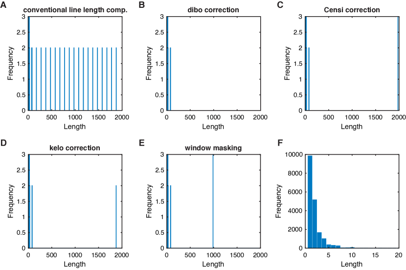
The real length of the border diagonals is unknown. Therefore, we are not able to assign their true length to them and, hence, one option to deal with the missing length regarding the line length histogram is setting their length to zero. That is, we simply discard all (semi-)border diagonals from $P(\ell)$ and, thus, avoid the broad line length distribution as exemplary shown in Fig. 3B. As desired, this results in a lowered entropy value, but also has some drawbacks. In case of a perfectly sampled stationary periodic signal (without any noise contamination and without effects due to tangential motion, cf. Sect.4) this method would empty the histogram $P(\ell)$ completely, leaving an undefined entropy (Figs. 8, 12, 13) and a mean and maximum line length of zero (cf. Fig. 4B for a result not corrected for tangential motion). In the following, we refer to this approach as dibo correction (DIscard BOrder diagonals).

3.1.2 Assign maximum line length to all border diagonals (Censi correction)

To avoid an empty diagonal line histogram, Censi et al.[18] suggested to assign all border diagonals the length of the main diagonal of the RP (line of identity). Sticking to the aforementioned example of a perfectly sampled and uncontaminated stationary periodic signal, this modification would result in a delta peak in $P(\ell)$ (cf. Fig. 4C for a result not corrected for tangential motion), and therefore a sound defined entropy value of zero as well as meaningful mean and maximal line length estimate (Figs. 8, 12, 13). For deterministic chaotic processes this correction scheme could underestimate the entropy, if the RP is smaller than the average length scale of the diagonal lines. Especially in a running window approach, this effect is assumed to be significant. We refer to this approach as Censi correction.

Figure 4: Diagonal line length histograms of the conventional line length computation (A) and of the presented correction schemes (B-E) for a monochromatic time-delay embedded sinusoidal with an oscillation period $T=100$ time units ($m=2$, $\tau=T/4$, same as in Figs. 2B and 3B). An enlargement of the histograms from panels A to D, focusing on the shorter line lengths, is presented in panel F. A corresponding enlargement of panel E does qualitatively look the same, but with reduced frequencies, due to the smaller effective window size (see text for details). For a better visibility we enlarged single bars in panels B to E and limited the view to a frequency range $[0~{}3]$ in panels A to E (in F the full range is used).

3.1.3 Keeping just the longest border diagonal (kelo correction)

In alternative to the correction in Sect. 3.1.1, all (semi-)border diagonals from $P(\ell)$ are discarded, but the longest one (cf. Fig. 4D). This approach would also avoid the broad line length distribution shown in Figs. 3B and  4A, but would leave a valid definition of the entropy, since $P(\ell)$ is not an empty set (cf. Figs. 8, 12, 13). The resulting entropy for the aforementioned example would be low. In contrast to the Censi correction, this approach would avoid the bias for deterministic chaotic processes when a windowing approach is applied. In the following, we refer to this approach as kelo correction (KEeping the LOngest border diagonal).

3.2 Alternative RP window shapes (window masking)

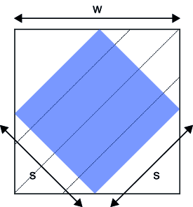
The origin of the border diagonals is related to a geometric difference between the RP and the diagonals. Therefore, a further approach to avoid the length bias of border diagonals is to apply a specific window to the RP which has the same geometric orientation as the diagonals. One realization of such a window is a 45° rotated cutout from the original RP (Fig. 5). Conventionally counting the lines of this rotated RP cutout preserves a delta peak distribution in $P(\ell)$ in case of a periodic signal (cf. Fig. 4E for a result not corrected for tangential motion). However, with this shape we loose $w^{2}-2s^{2}=w^{2}-\frac{1}{2}w^{2}=\frac{1}{2}w^{2}$ data points with respect to the original RP. Note that $s$ and $w$ in Fig. 5 imply a number of data points, meaning hypotenuse and catheti of an isosceles triangle have the same length ($w=\frac{s}{2}$). We argue that this approach could be rather useful in a running window approach over a global RP, where the size of the alternative shape could be chosen such that it contains as many data points as the classic, non-rotated, window. We refer to this approach as window masking. An alternative window shape would be a parallelogram with the top and bottom sides having the 45° direction [32].

Figure 5: Blue shaded alternative window shape with edge length $s$ of a $w\times w$ recurrence plot. $s$ and $w$ imply the number of RP matrix elements covered by the window shapes.

4 Tangential motion in Recurrence Quantification Analysis

Even though the considerations made in the preceding sections are valid and useful, the correction schemes presented in Sect. 3 most likely do not give the expected correction for the entropy of diagonal line lengths for experimental data, unless the data has been properly preprocessed. There are three reasons why the correction of the border diagonals in the diagonal line histogram $P(\ell)$ is not sufficient enough: (i) temporal correlations in the data, especially when highly sampled flow data is used, (ii) noise, and (iii) insufficient embedding of the time series at hand (if needed) combined with the effect of discretization and an inadequate choice of parameters needed to construct the RP (recurrence threshold method, recurrence threshold size, norm).

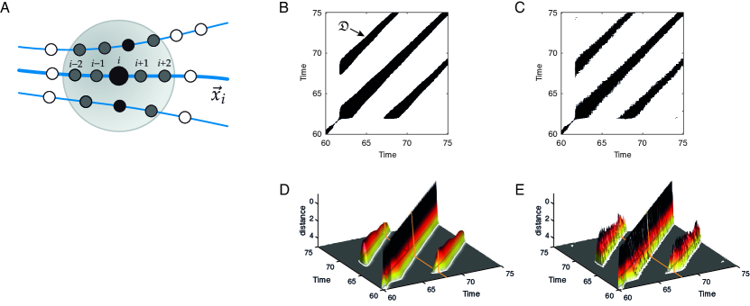
Temporal correlation means that states $\vec{x}_{j}$ preceding or succeeding a state $\vec{x}_{i}$ (or a recurring state $\vec{x}_{k}$ of $\vec{x}_{i}$), are very similar to this one and, hence, falling into the neighbourhood of $\vec{x}_{i}$ (or $\vec{x}_{k}$) and to be considered as recurrences, i.e., $R_{i,j}\colonequals 1$ for $j=[i-m,\ldots,i+n]$ or for $j=[k-m,\ldots,k+n]$ when $R_{i,k}\colonequals 1$ (Fig. 6A). This results in vertically extended sequences in the RP, i.e., thickening its diagonal lines. The thickening leads to an artificially enlarged number of diagonal lines, thus effecting the distribution $P(\ell)$, and is often referred to as tangential motion [33, 1]. Moreover, the thickening is not evenly distributed along a diagonal line (Fig. 6B). For border diagonals, this means that there are not only additional border diagonals (which could be handled by applying correction schemes as described in Sect. 3), but additional shorter diagonal lines, again leading to a broadening of the line length distribution $P(\ell)$ (Fig. 4, in particular panel F) and an elevated entropy $S$.

Additive noise causes the already thickened lines in the RP to appear more diffus (Fig. 6C,E). Technically speaking, the noise alters the phase space trajectory, causing the pairwise distances to randomly scatter about their true/noise free values and, thus, the histogram $P(\ell)$ gets enriched with small line lengths [34]. This eventually biases the RQA measures discussed in Sect. 2.

Figure 6: (A) Tangential motion, i.e., points of a trajectory preceding and succeeding a (recurring) state (gray), cause thickening of diagonal lines in the RP (B), (C). The thickening of diagonal lines can vary, e.g., as in this example of the Rössler system (noise free case in B and additive noise in C). The diagonal lines are more thick at the beginning and become less thick with time. A diagonal line in an RP (B), (C) denotes a range of distances in the distance matrix falling under a the recurrence threshold $\varepsilon$. Panels (D) and (E) show three “distance ranges” (we call such a range $\mathfrak{D}$ in the text) corresponding to the three lines in (B), (C) respectively. Shown is a colorcoded, thresholded distance matrix with reversed $z$-axis for a better visibility (increasing distances from top to bottom). The colormap encodes zero distance as black and the distance corresponding to the recurrence threshold as grey.

5 Correction schemes for reducing the effects of tangential motion

5.1 Perpendicular RP

A straightforward way to reduce the thickening of the diagonal lines from a theoretical perspective is the perpendicular RP, suggested by Choi et al. [35]

$$\textbf{R}_{i,j}^{\perp}(\varepsilon)=\Theta\left(\varepsilon-\|\vec{x}_{i}-\vec{x}_{j}\|\right)\cdot\delta\left(\dot{\vec{x}}_{i}\cdot(\vec{x}_{i}-\vec{x}_{j})\right),\qquad\vec{x}\in\mathbb{R}^{d}.$$ (7)

This RP contains only those points $\vec{x}_{j}$ that fall into the neighbourhood of $\vec{x}_{i}$ and lie in the ($d-1$)-dimensional subspace of $\mathbb{R}^{d}$ that is perpendicular to the phase space trajectory at $\vec{x}_{i}$. Although theoretically there is no need for an additional parameter in order to construct a perpendicular RP, in practical situations almost no points in $\mathbb{R}^{d}$ phase space end up on the mentioned ($d-1$)-dimensional subspace of $\vec{x}_{i}$ (Poincaré section), due to limited resolution (discretization) of the data. Hence, it is reasonable to introduce an additional threshold parameter $\varphi$, which allows points $\vec{x}_{j}$ to be considered as perpendicular to $\vec{x}_{i}$, if

$$\arccos{\frac{\dot{\vec{x}}_{i}\cdot(\vec{x}_{i}-\vec{x}_{j})}{|\dot{\vec{x}}_{i}|\cdot|(\vec{x}_{i}-\vec{x}_{j})|}}\in\Bigl{[}\left(\frac{\pi}{2}-\varphi\right),\left(\frac{\pi}{2}+\varphi\right)\Bigr{]}.$$ (8)

Thus, Eq. (7) transforms to

$${R}_{i,j}^{\perp}(\varepsilon,\varphi)=\Theta\left(\varepsilon-\|\vec{x}_{i}-\vec{x}_{j}\|\right)\cdot\Theta\left(\varphi-\biggl{|}\arccos{\frac{\dot{\vec{x}}_{i}\cdot(\vec{x}_{i}-\vec{x}_{j})}{|\dot{\vec{x}}_{i}|\cdot|(\vec{x}_{i}-\vec{x}_{j})|}}\biggl{|}-\frac{\pi}{2}\right),\qquad\vec{x}\in\mathbb{R}^{d}.$$ (9)

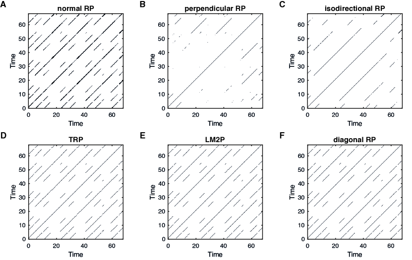
Figure 7B shows a perpendicular RP for a Rössler system (with parameters $a=0.15$, $b=0.2$, $c=10$, transients removed). For the estimation of the tangential at each point in phase space we used the reference point, its predecessor and its successor. We set the angle threshold to $\varphi=\frac{\pi}{12}$ ($=15$°).

5.2 Isodirectional RP

Requiring less computational effort, the iso-directional RP suggested by Horai et al. [36] also promises to cope with the tangential motion, but also inherits two additional parameters $T$ and $\varepsilon_{2}$ (Fig. 7C). In this approach two points in phase space are denoted recurrent, if their mutual distance falls within the recurrence threshold $\varepsilon$ and the distance of their trajectories throughout $T$ consecutive time steps falls within a recurrence threshold $\varepsilon_{2}$

$${R}_{i,j}^{\Nearrow}(\varepsilon,\varepsilon_{2},T)=\Theta(\varepsilon-\|\vec{x}_{i}-\vec{x}_{j}\|)\cdot\Theta(\varepsilon_{2}-\|(\vec{x}_{i+T}-\vec{x}_{i})-(\vec{x}_{j+T}-\vec{x}_{j})\|),\qquad\vec{x}\in\mathbb{R}^{d}.$$ (10)

We achieved decent results when choosing $T$ in the size of the decorrelation time (e.g., first minimum of the mutual information) and the second recurrence threshold as half of the size of the recurrence threshold $\varepsilon$, which determines the parent RP.

Figure 7: Different approaches for avoiding the effect of tangential motion in a recurrence plot (RP), exemplary shown for the Rössler system (with parameters $a=0.15$, $b=0.2$, $c=10$, sampling time $\Delta t=0.2$). (A) Normal RP with fixed recurrence threshold ensuring 4% global recurrence rate as a basis to all other RPs shown in this figure. (B) Perpendicular RP with angle threshold $\varphi=15$°, (C) isodirectional RP with $T=5$ [sampling units] and $\varepsilon_{2}=\varepsilon/2$, (D) true recurrence point RP (TRP) with $T_{\text{min}}=5$ [sampling units], which coincides with the first minimum of the mutual information, (E) thresholded local minima approach with two parameters (LM2P) and $\tau_{\text{m}}=5$, and (F) diagonal RP.

5.3 True recurrence point RP (TRP)

Inspired by the work of Gao [37], Ahlstrom et al. [38] compute a normal RP, Eq. (1), but only accept those points to be recurrent, which “first” enter the $\varepsilon$ neighbourhood shown in Fig. 6A. To ensure this, they first identify all points which fall into an $\varepsilon$-neighbourhood of a certain point $\vec{x}_{i}$

$$\zeta_{i}\equiv\{\vec{x}_{j_{1}},\vec{x}_{j_{2}},...~{}|{R}_{i,j_{k}}\colonequals 1\},$$ (11)

i.e., all points $j_{k}$ in column $i$ of the RP. The time difference of two consecutive recurrence points $\vec{x}_{j_{k}},\vec{x}_{j_{k+1}}$ is $\{T_{k}^{(1)}=j_{k+1}-j_{k}\}_{k\in\mathbb{N}}$ in units of the sampling time (recurrence times of first type [37]) and these correspond to the vertical distances between these points in column $i$ of the RP. They now discard all points from the RP, which vertical distance to its neighbouring point in a column is 1 and leaving all points with recurrence time larger than 1,

$$\zeta_{i}^{*}\equiv\{\vec{x}_{j_{1}},\vec{x}_{j_{2}},\ldots~{}|{R}_{i,j_{k}}\colonequals 1,~{}T_{k}^{(1)}>T_{\text{min}}\},\qquad T_{\text{min}}=1.$$ (12)

The authors call this modified RP a true recurrence point recurrence plot (TRP). This is different than simply discarding all points from the computations of Eq. (1) which fall within a certain time range $w_{\text{Theiler}}$ of the reference point (Theiler window [20])

$${R}_{i,j}(\varepsilon)=\Theta\left(\varepsilon-\|\vec{x}_{i}-\vec{x}_{j}\|\right),\qquad|i-j|>w_{\text{Theiler}},~{}\vec{x}\in\mathbb{R}^{d}.$$ (13)

To obtain a TRP, we suggest to discard all recurrence points with recurrence times greater than $w_{\text{Theiler}}$, i.e., $T_{\text{min}}=w_{\text{Theiler}}$ in Eq. (12). The Theiler window should be set in the order of the decorrelation time or the delay, if time delay embedding is used for reconstructing the phase space vectors from time series.

However, the TRP most often leads to disjoint, deviated diagonal line structures (Fig. 7D), which correspond to the white embraced lines in Fig. 6D, E.

An alternative would be to use the mid-points of the recurrence sequences. This would also correspond to recurrence times as discussed in [39]. In Subsec. 5.5, we will develop another correction scheme which is motivated by these mid-point based “true recurrences”.

5.4 RP by means of local minima

Another approach for reducing the effect of tangential motion and which shares the basic idea from the TRP approach, was introduced by Schultz et al. [22], who track the local minima of the distance matrix (corresponding to the maxima in Fig. 6D, E). Wendi & Marwan [23] then extended this idea in order to make the method more robust against noise. However, such local-minima based RP can contain bended or disrupted diagonal line structures. The key idea is to look for local minima in each column of the distance matrix, illustrated as an orange cross section in Fig. 6D, E. If such a local minimum is smaller than the recurrence threshold, then it is a recurrence (LocalMinimaThresholded, LMT). In the two-parameter approach (LM2P) [23] shown in Fig. 7E, there is an additional constraint for two consecutive local minima to be displaced by at least $\tau_{\text{m}}$ time steps.

5.5 Diagonal RP

We now propose an additional approach to cope with the tangential motion, which does not need any additional parameters and leads to an RP of straight, unbended diagonal line structures (Fig. 7F). We call this approach the diagonal RP, since it generates an RP with only diagonal line structures that are just one point thick.

A diagonal line in a RP corresponds to a connected region in the distance matrix with distances smaller than the recurrence threshold $\varepsilon$ (Fig. 6D, E, white embraced region). We call such region a “distance range” $\mathfrak{D}$. Typically, the larger $\varepsilon$ the larger the $\mathfrak{D}_{i}$’s in the RP. Moreover, tangential motion, noise and insufficient embedding affect the shape and width of the $\mathfrak{D}_{i}$’s. For the diagonal line based RQA measures we are interested in these ranges to be represented by single, connected diagonal lines in the corresponding RP. We choose the longest line of each $\mathfrak{D}_{i}$ to be its adequate representative in the RP. We define the “distance ranges” $\mathfrak{D}_{i}$ of an RP recursively as a set of adjacent diagonal lines $\mathcal{L}^{(m)}_{\ell_{m}}$ of length $\ell_{m}$ (cf. Eq. (4)), initializing with the longest line $\mathcal{L}^{(k)}_{\ell_{k}}$, for which $\ell_{k}={\max}(\ell\ :\ P(\ell)>0)$.

$$\mathfrak{D}_{i}\colonequals\{\mathcal{L}^{(k)}_{\ell_{k}},\mathcal{L}_{\ell_{m}}^{(m)}~{}|~{} \mathcal{L}_{\ell_{m}}^{(m)}~{}\curvearrowleft~{}\mathcal{L}_{\ell_{m-1}}^{(m-1)}~{}\curvearrowleft~{}\mathcal{L}_{\ell_{m-2}}^{(m-2)}~{}\curvearrowleft~{}...~{}\curvearrowleft~{}\mathcal{L}^{(k)}_{\ell_{k}}~{}\vee~{}$$

$$\mathcal{L}_{\ell_{m}}^{(m)}~{}\curvearrowright~{}\mathcal{L}_{\ell_{m-1}}^{(m-1)}~{}\curvearrowright~{}\mathcal{L}_{\ell_{m-2}}^{(m-2)}~{}\curvearrowright~{}...~{}\curvearrowright~{}\mathcal{L}^{(k)}_{\ell_{k}}\}$$ (14)

with the line-neighbour-relations $\curvearrowleft$ and $\curvearrowright$ defined by

$$\exists p\in[1,...,\ell_{m}]~{}\exists q\in[1,...,\ell_{k}]:\qquad\qquad\qquad\qquad\qquad\qquad\qquad\qquad$$

$$(i_{m},j_{m})_{p}\colonequals\begin{cases}(i_{k}+1,j_{k})_{q}\vee(i_{k},j_{k}+1)_{q},&\text{if}~{}\mathcal{L}_{\ell_{m}}^{(m)}\curvearrowleft\mathcal{L}_{\ell_{k}}^{(k)}\\ (i_{k}-1,j_{k})_{q}\vee(i_{k},j_{k}-1)_{q},&\text{if}~{}\mathcal{L}_{\ell_{m}}^{(m)}\curvearrowright\mathcal{L}_{\ell_{k}}^{(k)}\end{cases}$$ (15)

where $(i_{m},j_{m})_{p=[1,...,\ell_{m}]}$ denote the index tuples corresponding to lines $\mathcal{L}_{\ell_{m}}^{(m)}$ and $(i_{k},j_{k})_{q=[1,...,\ell_{k}]}$ denote the index tuples corresponding to the longest line $\mathcal{L}_{\ell_{k}}^{(k)}$. We then delete all lines contained in $\mathfrak{D}_{i}$ from the histogram $P(\ell)$ and define the next distance range $\mathfrak{D}_{i+1}$ with a new $\mathcal{L}_{\ell_{k^{\prime}}}^{(k^{\prime})}$ from the histogram and so on until $P(\ell)$ is an empty set.

We construct the new RP by keeping the longest line of each $\mathfrak{D}_{i}$ (all the $\mathcal{L}_{\ell_{k}}^{(k)}$’s). Denote the set of index tuples $(i,j)$ corresponding to the set of longest lines gained from the $\mathfrak{D}_{i}$’s as $\mathfrak{S}$, then

$${R}^{\nearrow}_{i,j}=\begin{cases}1,~{}\text{if}~{}(i,j)\in\mathfrak{S}\\ 0,~{}\text{otherwise}\end{cases}$$ (16)

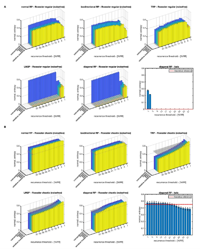
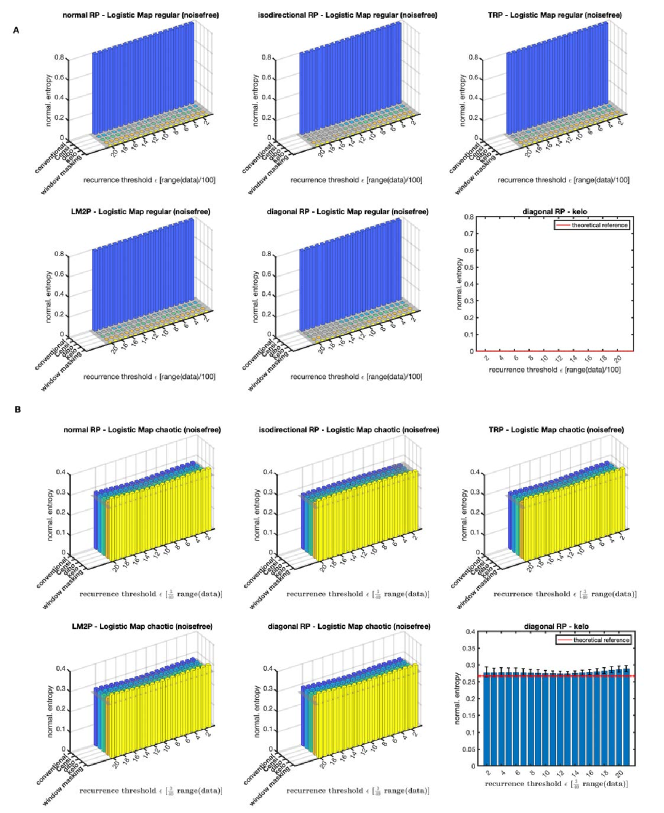
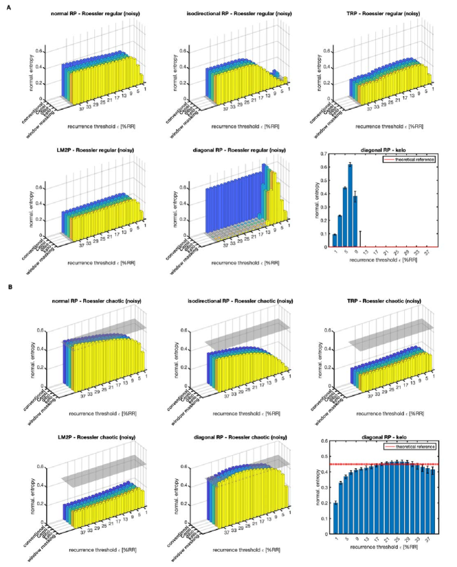
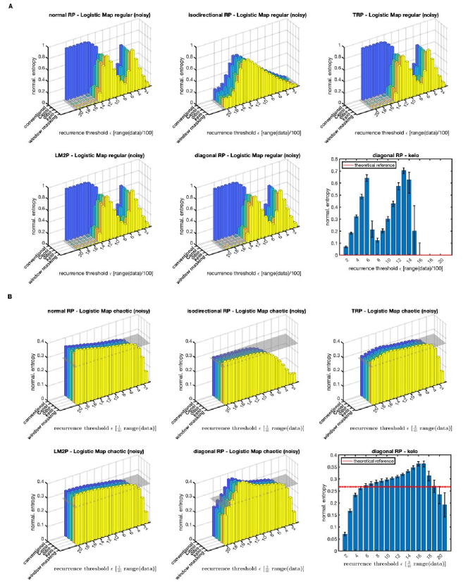
Note that this algorithm constricts clusters of adjacent recurrence points to a single diagonal line, representing this “distance range” $\mathfrak{D}$ (skeletonization). Although this method impresses with the absence of additional parameters, caution in its use is advised concerning the choice of the embedding parameters and the recurrence threshold. A wrong setup, specifically a too high recurrence threshold and/or a “wrong” time delay, could lead to an overall connected RP, which in turn would cause a diagonal RP consisting of just one single line in each triangle (if the main diagonal is discarded). However, concerning the sensitivity to the choice of the recurrence threshold, our numerical investigations suggest a rather low risk of this special case and a broad range of threshold values, which do work well (cf. Sect. 6, Sect. A and figures therein).

6 Results: Efficience of correction schemes

We now apply the correction schemes for counting diagonal lines (Sect. 3) and suppressing tangential motion (Sect. 5) on a time discrete as well as time continuous example, in order to test their ability to give valid estimates for the entropy of diagonal line lengths, Eq. (3). In case of the former we choose the Logistic map $x_{n+1}=rx_{n}(1-x_{n})$ with control parameter $r=3.5$, leading to regular limit cycle behavior, and control parameter $r=3.8$, where a chaotic regime is obtained. For the latter we show diagonal line length entropies of RPs of the Rössler system [40]

$$\dot{x} =-y-z$$

$$\dot{y} =x+ay$$ (17)

$$\dot{z} =b+z(x-c)$$

in two parameter configurations, also leading to regular limit cycle behavior ($a=0.15,b=c=10$) and chaotic motion ($a=0.15,b=0.2,c=10$) [41]. The results shown in this section are based on ensembles of 100 realizations of each parameter setting for the Rössler system and on ensembles of 1,000 realizations of each parameter setting for the Logistic map, gained from randomly chosen initial conditions out of a uniformly distributed interval $x_{0}\in[0,0.5]$ (Logistic map), $x(0),y(0),z(0)\in[0,2]$ (Rössler system). We numerically integrate the Rössler equations using the explicit Runge-Kutta (4,5) formalism (Dormand-Prince pair) as provided by the ode45-solver in MATLAB [42] with a fixed sampling time of $\Delta t=0.2$. For both systems we discard the first 2,500 data points as transients, keeping 1,000 (Logistic map) and 2,000 (Rössler) data points as the time series we base our further computations on. For estimating the entropy, we use the Maximum-Likelihood-estimator $p(\ell)~{}\widehat{=}~{}\hat{p}(\ell)=\frac{\#\text{number of lines of length}~{}\ell}{\#\text{number of all lines in the RP}}$ for the probabilities.

Generally, we expect (near-)zero entropy values for the regular regime setups and high(er) values for the chaotic regime setups for both considered examples in the noise free case (cf. Sect. 2). Moreover, we expect the correction schemes for counting diagonal lines (Sect. 3) to perform well in case of the Logistic map examples, due to the absence of tangential motion. For the flow data in the Rössler examples, we expect a combination of these correction schemes with the correction schemes for tangential motion described in Sect.  5 to give reasonable results. In order to validate our results we compute the diagonal line length entropy analytically for the mentioned cases. March et al. [27] gave an expression for this:

$$S_{\text{theoretical}}=K_{2}\left(\frac{1}{\gamma}-1\right)-\ln{\gamma}\quad,$$ (18)

with $\gamma=(1-e^{-K_{2}})$ and $K_{2}$ the correlation entropy. Practically we compute the largest Lyapunov exponent for our experimental settings [43] and use Pesin’s identity to get the Kolmogorov entropy $K_{1}$. Because the correlation entropy is a lower bound for the Kolmogorov entropy [44], we expect the reference values computed from Eq. (18) to give underestimated expectation values for the diagonal line length entropy.

Figure 8: Diagonal line length entropy (left panel) of the proposed diagonal recurrence plot ${R}^{\nearrow}$ (cf. Sect. 5.5) of the Rössler system (reddish) and the Logistic map (bluish) in a regular limit cycle regime (bright) as well as in a chaotic regime (dark). Shown are medians of the diagonal line length entropies gained from 1,000 realizations of the Logistic map and 100 realizations of the Rössler example, respectively, for the different line counting correction schemes described in Sect. 3. Errorbars indicate two standard deviations of these distributions. Black stars show medians of ensembles of 1,000 analytically computed values derived from Eq. (18) (its errorbars, as two standard deviations of the ensemble distribution, are barely visible and smaller than markers used). In the right panel the residuals to these underestimated expectation values are shown. Firstly, RPs were obtained with a fixed recurrence threshold corresponding to 19% recurrence rate in case of the Rössler examples and a fixed recurrence threshold corresponding to $1/10$ of the range of the underlying time series in case of the Logistic map examples (for noise free map data the $\varepsilon$-adjustment with respect to the global recurrence rate does not work properly). Then our proposed, parameter free correction scheme leading to the diagonal recurrence plot ${R}^{\nearrow}$ was applied. Results for a range of recurrence thresholds and for all tangential motion RP-correction schemes are shown in Fig. 12 and Fig. 13 in the Appendix A.

Figure 9: Diagonal line length entropy (left panel) based on the proposed line counting correction scheme $kelo$ (cf. Sect. 3.1.3) for the Rössler system (reddish) and the Logistic map (bluish) in a regular limit cycle regime (bright) as well as in a choatic regime (dark). Shown are medians of the diagonal line length entropies gained from 1,000 realizations of the Logistic map and 100 realizations of the Rössler example, respectively, for all the different tangential motion correction schemes described in Sect. 4, but the perpendicular recurrence plot ${R}^{\perp}$. Errorbars indicate two standard deviations of these distributions. Black stars show medians of ensembles of 1,000 analytically computed values derived from Eq. (18) (its errorbars, as two standard deviations of the ensemble distribution, are barely visible and smaller than markers used). In the right panel the residuals to these underestimated expectation values are shown. The normal RP with a fixed recurrence threshold corresponding to 19% recurrence rate in case of the Rössler examples and a fixed recurrence threshold corresponding to $1/10$ of the range of the underlying time series in case of the Logistic map examples (for noise free map data the $\varepsilon$-adjustment with respect to the global recurrence rate does not work properly) serves as a basis for the RP correction schemes shown here. Results for a range of recurrence thresholds and for all tangential motion RP-correction schemes are shown in Fig. 12 and Fig. 13 in the Appendix A.

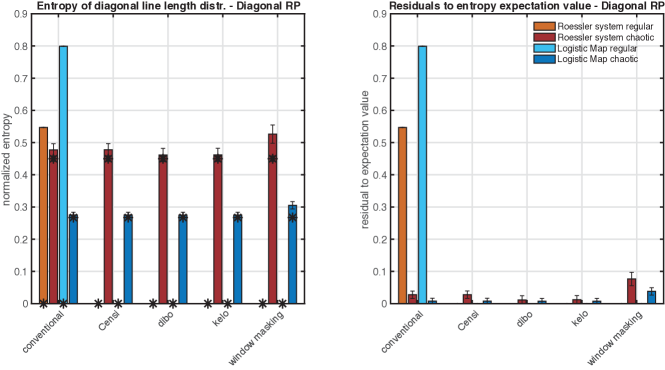
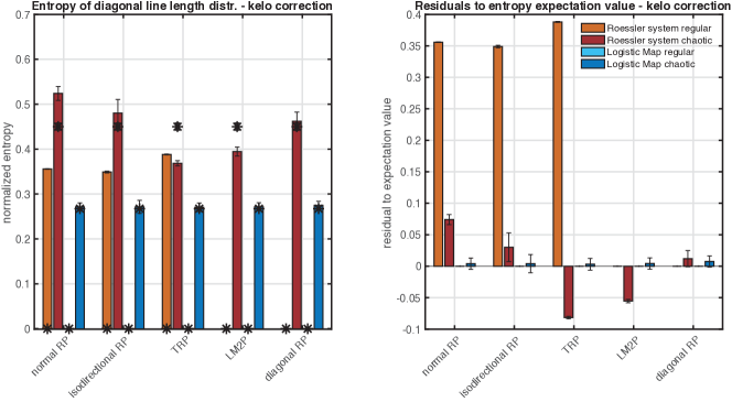
The results confirm our expectations (Fig. 8). While the conventional way of counting diagonal lines, where border effects are not taken into consideration, lead to counterintuitive behavior, all the described correction schemes are able to distinguish chaotic from regular regimes in both exemplary systems. In this laboratory, noise free conditions, the entropy estimates in case of the regular limit cycle regimes are zero (or in case of the $dibo$-correction scheme not defined, due to the absence of any diagonal line). For $dibo$ and $kelo$ the estimated values for the chaotic Rössler regime fall within the two standard deviation margin of the theoretical values, whereas Censi’s correction scheme comes very close and the windowshape correction scheme misses it by approx. 5%. Again, we have to stress that we expect the expectation values to be underestimated, i.e. we assume Censi’s method and the window masking do also perform well. Let us stick to the $kelo$ correction scheme for now and look how the different correction schemes for tangential motion perform (Fig. 9). First of all we have to mention that we were not able to produce any kind of reasonable estimates while using the perpendicular recurrence plot ${R}^{\perp}$, regardless of the angle threshold parameter. This straightforward approach is extremely sensitive to any kind of noise and to the sampling time of the system under observation. It needs a fairly high density of state space points, in order to yield a non empty RP and, thus, any meaningful diagonal line length entropy estimate. Hence, we skip this approach in our further analysis, especially the dependence of the shown results to the choice of the recurrence threshold and additive noise, but will discuss the performance of the perpendicular RP for a high sampled Rössler setup in the next subsection. For a general use, we cannot recommend the application of perpendicular RPs. Coming back to the results (Fig. 9), solely the LM2P approach and the diagonal RP perform as expected (zero-values in case of the regular regime setups and higher values for the chaotic regimes, clearly distinguishable). Only the proposed diagonal RP is able to give estimates within the errorbars of the theoretical values (which is why only this approach was selected for Fig. 8). Note that the reference values slightly underestimate the “true” value and we cannot quantitatively correct for this bias. As in Fig. 7, we set the parameters $T$, $T_{\text{min}}$ and $\tau_{\text{m}}$ to the corresponding first minimum of the auto mutual information and the second recurrence threshold for the isodirectional RP was again set to $\varepsilon_{2}=\varepsilon/2$, but we tried many parameter configurations.

6.1 Results for high sampled data and the effect of noise

For the sake of completeness and in order to investigate the behavior of our proposed methods under more realistic conditions, we now look at the noise corrupted Rössler system in the two dynamical regimes (Sect. 6), but with an increased sampling frequency (sampling time $\Delta t=0.08$) and with total lengths of the three numerically integrated time series of 10,000 (transients already removed). In this setup the perpendicular recurrence plot ${R}^{\perp}$ (Sect. 5.1) yields meaningful results (Fig. 10), and we compare its utility with respect to the estimation of the diagonal line length entropy to the normal RP and the novel diagonal recurrence plot ${R}^{\nearrow}$ (Sect. 5.5).

Figure 10: Cut outs of (A, D) the perpendicular recurrence plot ${R}^{\perp}$, (B, E) normal RP, and (C, F) the diagonal recurrence plot ${R}^{\nearrow}$ of the highly sampled Rössler system in chaotic regime (here with a sampling time of $\Delta t=0.02$). Top panels (A-C) show noise free cases, bottom panels (D-F) show their noise contaminated counterparts. Shown are results of additive white noise as 10% of the mean standard deviation of the multivariate signal gained from the numerical integration. Computations have been carried out by using a fixed recurrence threshold corresponding to 35% recurrence rate and an angle threshold $\varphi=15^{\circ}$ for ${R}^{\perp}$.

Figure 11: Normalized diagonal line length entropy estimates for all described correction schemes for counting diagonal lines (Sect. 3) based on the diagonal recurrence plot ${R}^{\nearrow}$ (Sect. 5.5) of the high sampled Rössler system as a function of the chosen minimal line length $\ell_{\text{min}}$. The top panels (A - chaotic motion , B - regular motion) show the noisefree case and in the bottom panels (C - chaotic motion, D - regular motion) the results for noise corrupted data are shown. We added noise from an auto-regressive (AR) process of second order as 20% of the mean standard deviation of the multivariate signal gained from the numerical integration (cf. Eq. (19)). The underlying RPs for obtaining ${R}^{\nearrow}$ were computed using a fixed recurrence threshold corresponding to 35% recurrence rate. The grey shaded areas show medians of ensembles of 1,000 analytically computed reference values for $K_{1}$ $\pm$ two standard deviations of these distributions transformed by using Eq. (18).

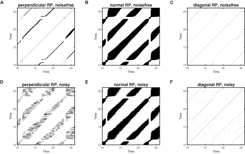
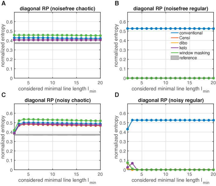
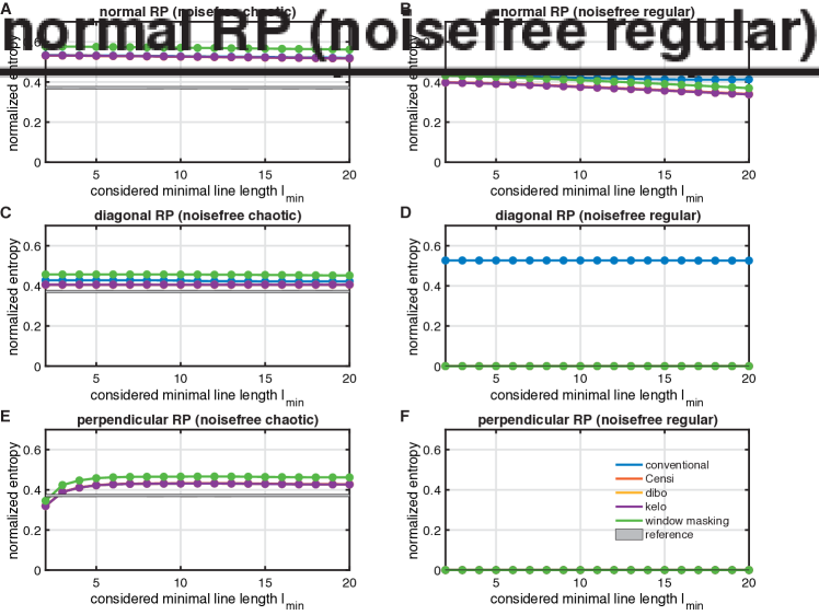
Figure 11 illustrates the capability of ${R}^{\nearrow}$ to cope with tangential motion, especially under noise. Due to a too high computational effort we did not compute an ensemble in this case as we did in the lower sampled cases, so the errorbars are missing. Here we added an auto regressive (AR) process of second order with an amplitude corresponding to 20% of the mean standard deviation of the multivariate signal.

$$x_{t}=a_{1}x_{t-1}+a_{2}x_{t-2}+\varepsilon_{t}\quad,$$ (19)

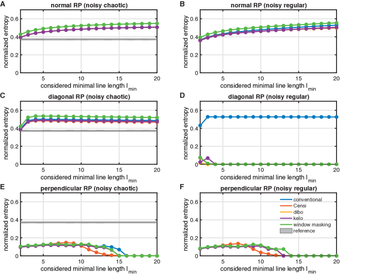
with parameters $a_{1}=0.7$, $a_{2}=0.15$ and $\varepsilon_{t}$ denotes a white noise process with zero mean and constant variance of unity. Outcomes for the normal RP and the perpendicular recurrence plot ${R}^{\perp}$ can be found in the Appendix (Figs. 16, 17). Additive white noise of the same magnitude gave similar results to the ones discussed here.

As expected from the examples in the last section, the diagonal RP approach performs well under noise free conditions and all, but the conventional line counting algorithms yield zero-value entropy estimates for the regular regime (panel B) and clearly non-zero entropies in case of the chaotic regime (panel A) close to the underestimated reference values. The perpendicular RP also performs well in noise free conditions (Fig. 16). Even the conventional line length counting leads to the desired zero entropy estimates in case of regular motion. In the presence of noise, however, ${R}^{\perp}$ is not able to distinguish regular from chaotic behavior (Fig. 17), whereas ${R}^{\nearrow}$ still performs well, giving almost the same results as in the noise free setup. The explanation can be found in considering the RPs (Fig. 10). For this noiselevel our proposed skeletonization approach (Fig. 10F) leaves small lines of maximum length 4 after its application to the noisy normal recurrence plot (Fig. 10E) as noise-leftovers. The appearance of these lines is not a result of the dynamics itself. Noise enriches the RP and its corresponding diagonal line histogram with small line lengths depending on the noiselevel ([34], Fig. 10, Fig. 2A, Fig. 3A). By increasing the minimum line length one gradually discards the majority of the lines contained in the histogram and, thus, increases the prominence of larger line lengths for the computation of the entropy. For a regular regime, the distribution of lines of intermediate length is broader for all the correction schemes, but the diagonal RP. Therefore an increasing minimal line length increases the entropy in the presence of noise for all the correction schemes, but the diagonal RP (cf. Fig. 17). In case of a chaotic regime the distribution of diagonals due to the dynamics is broader anyway (Fig. 2C, Fig. 3C) leading to the same effect.

When increasing the minimal line length for the diagonal RP, the entropy estimates stay more or less constant after a certain, sufficiently high, minimum line length, which depends on the noiselevel (Fig. 11C, D). The offset to the underestimated reference value for the chaotic case grows for increasing noiselevels. Note that the effect of additive noise is harder to tackle for the tangential motion correction schemes for high sampled data like in this case, than it is for lower sampled examples as discussed in Sect. 6. The higher the sampling, the finer the ramification of distance ranges $\mathfrak{D}_{i}$ (thickened diagonal lines). Results for all correction schemes for a wide range of the recurrence thresholds and under the influence of white noise for the lower sampled situation can be found in the Appendix (Figs. 14 and 15).

7 Discussion

In this letter we investigated the effect of the finite size of a recurrence plot on its diagonal line length based quantification. Specifically, we showed how these border effects influence the diagonal line length entropy and proposed three new line length counting correction schemes, which take these effects into account (cf. Subsects. 3.1.1, 3.1.3, 3.2) and systematically compared them to an already proposed correction by Censi et al. [18] (Subsect. 3.1.2). It turned out that for noise free or slightly noise corrupted map data all these correction methods solve the problem of the biased diagonal line length entropy due to lines cut by the borders of the RP. However, for flow data the effect of tangential motion has a much bigger influence on the entropy bias than the border effects. Therefore, we systematically compared already proposed ideas to handle tangential motion and proposed a new, parameter free method, the diagonal RP (cf. Sect. 5.5). It can properly tackle the tangential motion effects and yield, in combination with the border effect correction schemes, meaningful estimates for the diagonal line length entropy. We have to emphasize that this method, in contrast to other suggested ideas, also works for noise contaminated data, is not sensitive to the particular choice of the recurrence threshold, does not introduce any additional parameter, and is, therefore, easy to use. In case of a noise corrupted flow-like signal the diagonal line length entropy approaches its constant expectation value for sufficiently high choices of the minimal line length, when the diagonal RP together with Censi’s or our propsed border effect correction schemes is used. Fairly high recurrence thresholds (>10% recurrence rate) favour the diagonal RP method for intermediate or high noise levels.

Appendix A Sensitivity of the results to the recurrence threshold

Figure 12: Diagonal line length entropy estimates as a function of the recurrence threshold $\varepsilon$. Shown are results for all described correction schemes for counting diagonal lines (Sect. 3) and suppressing tangential motion (Sect. 4), except the perpendicular recurrence plot ${R}^{\perp}$. In the top panel (A) median diagonal line length entropy values gained from 100 realizations of the noise free regular limit cycle regime of the Rössler system are shown, whereas the bottom panel (B) shows its chaotic regime counterpart, see text in Sect. 6 for details. The grey-shaded surface denotes the theoretical expectation value (median) computed from Eq. (18). Results for the diagonal RP and the kelo correction scheme are shown in the bottom right subplot, which is a cutout of the orange bars in the bottom center subplot, here including errorbars as two standard deviations from the computed ensemble.

Figure 13: Diagonal line length entropy estimates as a function of the recurrence threshold $\varepsilon$. Shown are results for all described correction schemes for counting diagonal lines (Sect. 3) and suppressing tangential motion (Sect. 4), except the perpendicular recurrence plot ${R}^{\perp}$. In the top panel (A) median diagonal line length entropy values gained from 1,000 realizations of the noise free regular limit cycle regime of the Logistic map are shown, whereas the bottom panel (B) shows its chaotic regime counterpart, see text in Sect. 6 for details. The grey-shaded surface denotes the theoretical expectation value (median) computed from Eq. (18). Results for the diagonal RP and the kelo correction scheme are shown in the bottom right subplot, which is a cutout of the orange bars in the bottom center subplot, here including errorbars as two standard deviations from the computed ensemble.

Figure 14: Diagonal line length entropy estimates as a function of the recurrence threshold $\varepsilon$. Shown are results for all described correction schemes for counting diagonal lines (Sect. 3) and suppressing tangential motion (Sect. 4), except the perpendicular recurrence plot ${R}^{\perp}$. In the top panel (A) median diagonal line length entropy values gained from 100 realizations of the additive noise contaminated regular limit cycle regime of the Rössler system are shown, whereas the bottom panel (B) shows its chaotic regime counterpart, see text in Sect. 6.1 for details. Here, we added white noise as 10% of the mean standard deviation of the multivariate signal gained from the numerical integration. The grey-shaded surface denotes the theoretical expectation value (median) computed from Eq. (18). Results for the diagonal RP and the kelo correction scheme are shown in the bottom right subplot, which is a cutout of the orange bars in the bottom center subplot, here including errorbars as two standard deviations from the computed ensemble.

Figure 15: Diagonal line length entropy estimates as a function of the recurrence threshold $\varepsilon$. Shown are results for all described correction schemes for counting diagonal lines (Sect. 3) and suppressing tangential motion (Sect. 4), except the perpendicular recurrence plot ${R}^{\perp}$. In the top panel (A) median diagonal line length entropy values gained from 1,000 realizations of the additive noise contaminated regular limit cycle regime of the Logistic map are shown, whereas the bottom panel (B) shows its chaotic regime counterpart, see text in Sect. 6.1 for details. Here, we added white noise as 10% of the standard deviation of the time series. The grey-shaded surface denotes the theoretical expectation value (median) computed from Eq. (18). Results for the diagonal RP and the kelo correction scheme are shown in the bottom right subplot, which is a cutout of the orange bars in the bottom center subplot, here including errorbars as two standard deviations from the computed ensemble.

Appendix B Sensitivity of the results to noise

Figure 16: Normalized diagonal line length entropy estimates as a function of the minimum line length $\ell_{min}$ for noisefree data from the high sampled Rössler system (cf. Sect. 6.1). In the left panels (A, C, E) the underlying system exhibits chaotic dynamics, whereas the right panels (B, D, F) show their regular counterparts. The normal RPs (A, B) and the perpendicular RPs (E, F) were constructed using a fixed recurrence threshold corresponding to 35% recurrence rate. The normal RPs served as input for obtaining the diagonal RPs ${R}^{\nearrow}$ (C, D) and for the computation of the perpendicular RPs ${R}^{\perp}$ we used an angle threshold $\varphi=15$°. The grey shaded areas show medians of ensembles of 1,000 analytically computed reference values for $K_{1}$ $\pm$ two standard deviations of these distributions transformed by using Eq. (18).

Figure 17: Normalized diagonal line length entropy estimates as a function of the minimum line length $\ell_{min}$ for noise corrupted data from the high sampled Rössler system (cf. Sect. 6.1). We added noise from an auto-regressive (AR) process of second order as 20% of the mean standard deviation of the multivariate signal gained from the numerical integration (cf. Eq. (19)). In the left panels (A, C, E) the underlying system exhibits chaotic dynamics, whereas the right panels (B, D, F) show their regular counterparts. The normal RPs (A, B) and the perpendicular RPs (E, F) were constructed using a fixed recurrence threshold corresponding to 35% recurrence rate. The normal RPs served as input for obtaining the diagonal RPs ${R}^{\nearrow}$ (C, D) and for the computation of the perpendicular RPs ${R}^{\perp}$ we used an angle threshold $\varphi=15$°. The grey shaded areas show medians of ensembles of 1,000 analytically computed reference values for $K_{1}$ $\pm$ two standard deviations of these distributions transformed by using Eq. (18).

References

- [1] N. Marwan, M. C. Romano, M. Thiel, J. Kurths, Recurrence Plots for the Analysis of Complex Systems, Physics Reports 438 (5–6) (2007) 237–329. doi:10.1016/j.physrep.2006.11.001.
- [2] C. L. Webber, Jr., N. Marwan, Recurrence Quantification Analysis – Theory and Best Practices, Springer, Cham, 2015. doi:10.1007/978-3-319-07155-8.
- [3] N. Marwan, N. Wessel, U. Meyerfeldt, A. Schirdewan, J. Kurths, Recurrence Plot Based Measures of Complexity and its Application to Heart Rate Variability Data, Physical Review E 66 (2) (2002) 026702. doi:10.1103/PhysRevE.66.026702.
- [4] Z. O. Guimarães-Filho, I. L. Caldas, R. L. Viana, J. Kurths, I. C. Nascimento, Y. K. Kuznetsov, Recurrence quantification analysis of electrostatic fluctuations in fusion plasmas, Physics Letters A 372 (7) (2008) 1088–1095. doi:10.1016/j.physleta.2007.07.088.
- [5] A. Facchini, F. Rossi, C. Mocenni, Spatial recurrence strategies reveal different routes to Turing pattern formation in chemical systems, Physics Letters A 373 (46) (2009) 4266–4272. doi:10.1016/j.physleta.2009.09.049.
- [6] C. L. Webber, Jr., N. Marwan, A. Facchini, A. Giuliani, Simpler methods do it better: Success of Recurrence Quantification Analysis as a general purpose data analysis tool, Physics Letters A 373 (2009) 3753–3756. doi:10.1016/j.physleta.2009.08.052.
- [7] K. Guhathakurta, B. Bhattacharya, A. R. Chowdhury, Using recurrence plot analysis to distinguish between endogenous and exogenous stock market crashes, Physica A 389 (9) (2010) 1874–1882. doi:10.1016/j.physa.2009.12.061.
- [8] Y. Hirata, Y. Shimo, H. L. Tanaka, K. Aihara, Chaotic Properties of the Arctic Oscillation Index, SOLA 7 (2011) 33–36. doi:10.2151/sola.2011-009.
- [9] N. P. Subramaniyam, J. Hyttinen, Characterization of dynamical systems under noise using recurrence networks: Application to simulated and EEG data, Physics Letters A 378 (46) (2014) 3464–3474. doi:10.1016/j.physleta.2014.10.005.
- [10] M. S. Santos, J. D. Szezech, A. M. Batista, I. L. Caldas, R. L. Viana, S. R. Lopes, Recurrence quantification analysis of chimera states, Physics Letters A 379 (37) (2015) 2188–2192. doi:10.1016/j.physleta.2015.07.029.
- [11] O. Kopáček, V. Karas, J. Kovář, Z. Stuchlík, Transition from regular to chaotic circulation in magnetized coronae near compact objects, The Astrophysical Journal 722 (2) (2010) 1240. doi:10.1088/0004-637X/722/2/1240.
- [12] V. Mitra, A. Sarma, M. S. Janaki, A. N. Sekar Iyengar, B. Sarma, N. Marwan, J. Kurths, P. K. Shaw, D. Saha, S. Ghosh, Order to chaos transition studies in a DC glow discharge plasma by using recurrence quantification analysis, Chaos, Solitons & Fractals 69 (2014) 285–293. doi:10.1016/j.chaos.2014.10.005.
- [13] V. Nair, G. Thampi, R. I. Sujith, Intermittency route to thermoacoustic instability in turbulent combustors, Journal of Fluid Mechanics 756 (2014) 470–487. doi:10.1017/jfm.2014.468.
- [14] J. P. Zbilut, C. L. Webber, Jr., Embeddings and delays as derived from quantification of recurrence plots, Physics Letters A 171 (3–4) (1992) 199–203. doi:10.1016/0375-9601(92)90426-M.
- [15] L. L. Trulla, A. Giuliani, J. P. Zbilut, C. L. Webber, Jr., Recurrence quantification analysis of the logistic equation with transients, Physics Letters A 223 (4) (1996) 255–260. doi:10.1016/S0375-9601(96)00741-4.
- [16] J. F. Donges, R. V. Donner, K. Rehfeld, N. Marwan, M. H. Trauth, J. Kurths, Identification of dynamical transitions in marine palaeoclimate records by recurrence network analysis, Nonlinear Processes in Geophysics 18 (2011) 545–562. doi:10.5194/npg-18-545-2011.
- [17] D. Eroglu, T. K. D. Peron, N. Marwan, F. A. Rodrigues, L. d. F. Costa, M. Sebek, I. Z. Kiss, J. Kurths, Entropy of weighted recurrence plots, Physical Review E 90 (2014) 042919. doi:10.1103/PhysRevE.90.042919.
- [18] F. Censi, G. Calcagnini, S. Cerutti, Proposed corrections for the quantification of coupling patterns by recurrence plots, IEEE Transactions on Biomedical Engineering 51 (5) (2004) 856–859.
- [19] N. Marwan, How to avoid potential pitfalls in recurrence plot based data analysis, International Journal of Bifurcation and Chaos 21 (4) (2011) 1003–1017. doi:10.1142/S0218127411029008.
-
[20]
J. Theiler, Spurious
dimension from correlation algorithms applied to limited time-series data,
Phys. Rev. A 34 (1986) 2427–2432.
doi:10.1103/PhysRevA.34.2427.
URL https://link.aps.org/doi/10.1103/PhysRevA.34.2427 - [21] A. Facchini, H. Kantz, Curved structures in recurrence plots: The role of the sampling time, Physical Review E 75 (2007) 036215. doi:10.1103/PhysRevE.75.036215.
- [22] A. Schultz, Y. Zou, N. Marwan, M. T. Turvey, Local Minima-based Recurrence Plots for Continuous Dynamical Systems, International Journal of Bifurcation and Chaos 21 (4) (2011) 1065–1075. doi:10.1142/S0218127411029045.
[23]
D. Wendi, N. Marwan, Extended
recurrence plot and quantification for noisy continuous dynamical systems,
Chaos: An Interdisciplinary Journal of Nonlinear Science 28 (8) (2018)
085722.
arXiv:https://doi.org/10.1063/1.5025485, doi:10.1063/1.5025485.
URL https://doi.org/10.1063/1.5025485 - [24] J.-P. Eckmann, S. Oliffson Kamphorst, D. Ruelle, Recurrence Plots of Dynamical Systems, Europhysics Letters 4 (9) (1987) 973–977. doi:10.1209/0295-5075/4/9/004.
- [25] P. Faure, H. Korn, A new method to estimate the Kolmogorov entropy from recurrence plots: its application to neuronal signals, Physica D 122 (1–4) (1998) 265–279. doi:10.1016/S0167-2789(98)00177-8.
- [26] M. Thiel, M. C. Romano, P. L. Read, J. Kurths, Estimation of dynamical invariants without embedding by recurrence plots, Chaos 14 (2) (2004) 234–243. doi:10.1063/1.1667633.
- [27] T. K. March, S. C. Chapman, R. O. Dendy, Recurrence plot statistics and the effect of embedding, Physica D 200 (1–2) (2005) 171–184. doi:10.1016/j.physd.2004.11.002.
- [28] M. Thiel, M. C. Romano, J. Kurths, Analytical Description of Recurrence Plots of white noise and chaotic processes, Izvestija vyssich ucebnych zavedenij/ Prikladnaja nelinejnaja dinamika – Applied Nonlinear Dynamics 11 (3) (2003) 20–30.
- [29] C. L. Webber, Jr., J. P. Zbilut, Dynamical assessment of physiological systems and states using recurrence plot strategies, Journal of Applied Physiology 76 (2) (1994) 965–973.
- [30] D. Wendi, N. Marwan, B. Merz, In search of determinism-sensitive region to avoid artefacts in recurrence plots, International Journal of Bifurcation and Chaos 28 (1) (2018) 1850007. doi:10.1142/S0218127418500074.
- [31] J. P. Zbilut, A. Giuliani, C. L. Webber, Jr., Recurrence quantification analysis and principal components in the detection of short complex signals, Physics Letters A 237 (3) (1998) 131–135. doi:10.1016/S0375-9601(97)00843-8.
- [32] J. Donath, Untersuchung alternativer Zeitfensterformen für die quantitative Rekurrenzanalyse anhand von Modellsystemen und Klimadaten, Bachelor thesis, Humboldt Universität zu Berlin (May 2016).
- [33] J. B. Gao, H. Q. Cai, On the structures and quantification of recurrence plots, Physics Letters A 270 (1–2) (2000) 75–87. doi:10.1016/S0375-9601(00)00304-2.
- [34] M. Thiel, M. C. Romano, J. Kurths, R. Meucci, E. Allaria, F. T. Arecchi, Influence of observational noise on the recurrence quantification analysis, Physica D 171 (3) (2002) 138–152. doi:10.1016/S0167-2789(02)00586-9.
- [35] J. M. Choi, B. H. Bae, S. Y. Kim, Divergence in perpendicular recurrence plot; quantification of dynamical divergence from short chaotic time series, Physics Letters A 263 (4–6) (1999) 299–306. doi:10.1016/S0375-9601(99)00751-3.
- [36] S. Horai, T. Yamada, K. Aihara, Determinism Analysis with Iso-Directional Recurrence Plots, IEEE Transactions - Institute of Electrical Engineers of Japan C 122 (1) (2002) 141–147.
- [37] J. B. Gao, Recurrence Time Statistics for Chaotic Systems and Their Applications, Physical Review Letters 83 (16) (1999) 3178–3181. doi:10.1103/PhysRevLett.83.3178.
- [38] C. Ahlstrom, P. Hult, P. Ask, Thresholding distance plots using true recurrence points, Proceedings of the IEEE Conference on Acoustics, Speech and Signal Processing (ICASSP 2006) 3 (1660747) (2006) III688–III691. doi:10.1109/ICASSP.2006.1660747.
- [39] E. J. Ngamga, D. V. Senthilkumar, A. Prasad, P. Parmananda, N. Marwan, J. Kurths, Distinguishing dynamics using recurrence-time statistics, Physical Review E 85 (2) (2012) 026217. doi:10.1103/PhysRevE.85.026217.
[40]
O. Roessler,
An
equation for continuous chaos, Physics Letters A 57 (5) (1976) 397 – 398.
doi:https://doi.org/10.1016/0375-9601(76)90101-8.
URL http://www.sciencedirect.com/science/article/pii/0375960176901018 -
[41]
R. Barrio, F. Blesa, S. Serrano,
Qualitative
analysis of the rössler equations: Bifurcations of limit cycles and chaotic
attractors, Physica D: Nonlinear Phenomena 238 (13) (2009) 1087 – 1100.
doi:https://doi.org/10.1016/j.physd.2009.03.010.
URL http://www.sciencedirect.com/science/article/pii/S0167278909000864 - [42] L. F. Shampine, M. W. Reichelt, The matlab ode suite, SIAM Journal on Scientific Computing 18 (1997) 1–22.
- [43] G. Datseries, Dynamicalsystems.jl: A julia software library for chaos and nonlinear dynamics., Journal of Open Source Software 3(23) (2018) 598. doi:10.21105/joss.00598.
- [44] P. Grassberger, I. Procaccia, Estimation of the Kolmogorov entropy from a chaotic signal, Physical Review A 9 (1–2) (1983) 2591–2593. doi:10.1103/PhysRevA.28.2591.
[45]
K. H. Kraemer,
hkraemer/Border-effect-corrections-for-diagonal-line-based-recurrence-quantification-analysis-measures:
MATLAB routines for RQA border effect and tangential motion correction
(Jun. 2019).
doi:10.5281/zenodo.3384892.
URL https://doi.org/10.5281/zenodo.3384892