Analysis of Regression Tree Fitting Algorithms
in Learning to Rank

Abstract

In learning to rank area, industry-level applications have been dominated by gradient boosting framework, which fits a tree using least square error principle. While in classification area, another tree fitting principle, weighted least square error, has been widely used, such as LogitBoost and its variants. However, there is a lack of analysis on the relationship between the two principles in the scenario of learning to rank. We propose a new principle named least objective loss based error that enables us to analyze the issue above as well as several important learning to rank models. We also implement two typical and strong systems and conduct our experiments in two real-world datasets. Experimental results show that our proposed method brings moderate improvements over least square error principle.

1 Introduction

Top practical learning to ranking systems are adopting gradient boosting framework and using regression trees as weak learners. These systems performed much better than linear systems on real-world datasets, such as Yahoo challenge 2010 ([4]), and Microsoft 30K ([21]). Among these systems, LambdaMART ([24, 3]), a pair-wise based model, gained an excellent reputation in Yahoo challenge; MART ([9]), a point-wise based, is a regression model which utilizes least square loss as objective loss function, and McRank ([15]), a point-wise based, uses multi-class classification technique and converts predictions into ranking. For industry application, gradient boosting combined with regression trees appears to be a standard practice.

An important finding was made in the work of ([6, 15]) that has created a bridge between learning to rank and classification. They proved that an important measure NDCG in learning to rank could be bounded by multi-class classification error. This insight opens a door for learning to rank, as we could borrow state-of-the-art classification techniques.

Least square error (SE) principle in fitting a regression tree only utilizes the first-order information of objective loss function, while in multi-class classification area, there is a work that fits a regression tree by use of second-order information besides that. Their tree fitting principle is called weighted least square error (WSE). LogitBoost ([8]) and its robust versions ([13, 14]) are examples. A comparison between gradient boosting using SE and LogitBoost using WSE for classification task ([9]) shows that the latter is slightly better. As WSE is empirically considered as unstable in practice ([8, 14, 9]), [14] obtained a stable form of WSE, called RWSE.

Figure 1: Dark shadow marked ellipses denote tree fitting principles, and rectangles denote ranking models. SE: least square error; RWSE: robust weighted square error; OLE: objective loss based error in this paper. All real-line arrows denote known relations, and dotted-line arrows denote our contribution.

However, both WSE and RWSE have no clear theoretical explanation, and somewhat hard to understand. As a result, Li thus proposed an interesting question in Section 2.3 of ([14]): in determining the output of a leaf of a regression tree, the one-step Newton formula from gradient boosting coincides with the weighted averaging from WSE. Moreover, RWSE looks concise, which might be mistaken to apply to any ranking model besides LogitBoost and its variants. These issues drive us to consider from another point of view.

We propose a general regression tree fitting principle for ranking models, called least objective loss based error (OLE). It only requires simple computation to derive exact formula and is easy to understand. Under this principle, we first clearly answer the aforementioned question, and then analyze a variety of ranking systems to build a relationship between SE, (R)WSE and OLE (Figure 1). Experiments in real-world datasets also show moderate improvements.

2 Background

Given a set of queries $\mathbf{Q}=\{q_{1},\ldots,q_{|\mathbf{Q}|}\}$, each query $q_{i}$ is associated with a set of candidate relevant documents $\mathbf{D}_{i}=\{d_{1}^{i},\ldots,d_{|\mathbf{D}_{i}|}^{i}\}$ and a corresponding vector of relevance scores $\mathbf{Y}_{i}=\{y_{i}(d_{1}^{i}),\ldots,y_{i}(d_{|\mathbf{D}_{i}|}^{i})\}$ for each $\mathbf{D}_{i}$. The relevance score is usually an integer, assuming $0\leq y\leq K$. Greater value means more related for the document to the query. An $M$-dimensional feature vector $\mathbf{h}(d)=[h_{1}(d|q),\ldots,h_{M}(d|q)]^{T}$ is created for each query-document pair, where $h_{t}(\cdot)$s are predefined feature functions, which usually return real values.

A ranking function $f$ is designed to score each query-document pair, and the documents associated with the same query are ranked by their scores and returned to users. Since these documents have a fixed ground truth rank with its corresponding query, our goal is to find an optimal ranking function which returns such a rank of related documents that is as close to the ground truth rank as possible. Industry-level applications often adopt regression trees to construct the ranking function, and use Newton Formula to calculate the output values of leaves of trees.

Since fitting a regression tree is conducted node by node, in this paper we only discuss the differences of algorithms running on each node. We call them node-splitting algorithms. To distinguish them from the objective loss functions of ranking models, we refer to the loss of each node-splitting algorithm as the "error". For example, square error (Section 2.1), (robust) weighted square error (Section 2.2.1, 2.2.2), and the objective loss based error (Section 3.1) proposed in this work. Obviously, if there is a minor difference in the split of a tree node for two node-splitting algorithms, they would lead to two totally different regression trees.

Several measures have been used to quantify the quality of the rank with respect to a ground-truth rank such as NDCG, ERR, MAP etc. In this paper, we use the most popular NDCG and ERR ([4]) as the performance measures.

2.1 Square Error (SE) in Gradient Boosting

We regard gradient boosting ([9]) as a general framework for function approximation, and it is applicable for any differentiable loss function. Combining with regression trees as weak learners has been the most successful application in learning to rank area.

Gradient boosting iteratively finds an additive predictor $f(\cdot)\in\mathcal{H}$, which minimizes the loss function $\mathcal{L}$. At the $t$th iteration, a new weak learner $g_{t}(\cdot)$ is selected to add to current predictor $f_{t}(\cdot)$. Then

$$f_{t+1}(\cdot)=f_{t}(\cdot)+\alpha g_{t}(\cdot)$$ (1)

where $\alpha$ is the learning rate.

In gradient boosting, $g_{t}(\cdot)$ is chosen as the one most parallel to pseudo-response $r(\cdot)$, which is defined as the negative derivative of the loss function in functional space $\mathcal{H}$.

$$r(\cdot)=-\mathcal{L}^{\prime}(f_{t}(\cdot))$$ (2)

In practice, the globally optimal $g_{t}(\cdot)$ usually can not be obtained, then we turn to operations on each tree node to fit a sub-optimal tree. In one node, we enumerate all possible feature-threshold pairs, and then the best one is selected to conduct binary splitting. This procedure recursively iterates on its child nodes until reaching a predefined condition.

Regarding a feature, suppose a threshold $v$ to split samples on the current node into two parts. The samples, whose feature values are less than $v$, are denoted as $\mathbf{D}_{l}$, and others are denoted as $\mathbf{D}_{r}$. The squared error is defined as

$$SE(v)=\sum_{d\in\mathbf{D}_{l}}(r(d)-\overline{r_{1}})^{2}+\sum_{d\in\mathbf{D}_{r}}(r(d)-\overline{r_{2}})^{2}$$ (3)

where $\overline{r_{1}}$, $\overline{r_{2}}$ are average pseudo-response of samples on the left and right respectively.

The complexity of a regression tree could be controlled by limiting the tree height or leaf number. In learning to rank, the latter is more flexible, and adopted in this work by default.

2.2 Weighted Square Error in Classification

[6] proved that the negative unnormalized NDCG value is upper-bounded by multi-class classification error, where NDCG is an important measure in learning to rank. Thus [15] proposed a multi-class classification based ranking systems called McRank in gradient boosting framework.

McRank utilizes classic logistic regression, which models class probability $p_{k}(d)$ as

$$p_{k}(d)=p(y(d)=k)=\frac{\exp f^{k}(d)}{\sum_{c=0}^{K}\exp f^{c}(d)}$$ (4)

where $f^{c}(\cdot)$ is an additive predictor function for the $c$th class.

The objective loss function is the negative log-likelihood, defined as

$$\mathcal{L}=-{\sum_{d}}{\sum_{k=0}^{K}\,}\textrm{I}(y(d)=c)\log p_{k}(d)$$ (5)

where $\textrm{I}(\cdot)$ is an indicator function.

2.2.1 Weighted Square Error (WSE)

In classification, this loss function (Eqn. 5) resulted in the well-known system LogitBoost, which first used WSE to fit a regression tree. WSE utilizes both first- and second- order derivative information.

WSE uses a different definition of the response value $r(\cdot)$ from that in SE (Eqn. 2), and defines an extra weight $w(\cdot)$ for each sample.

$$\begin{array}[]{clc}r(\cdot)&=&-\mathcal{L}^{\prime}(f_{t}(\cdot))/\mathcal{L}^{\prime\prime}(f_{t}(\cdot))\\ w(\cdot)&=&\mathcal{L}^{\prime\prime}(f_{t}(\cdot))\end{array}$$ (6)

The splitting principle is minimizing the following weighted error

$$WSE(v)=\left[\sum_{d\in\mathbf{D}_{l}}w(d)(r(d)-\overline{r_{1}})^{2}+\sum_{d\in\mathbf{D}_{r}}w(d)(r(d)-\overline{r_{2}})^{2}\right]-\sum_{d\in\mathbf{D}}w(d)(r(d)-\bar{r})^{2}$$ (7)

where

$$\overline{r_{1}}=\frac{\sum_{d\in\mathbf{D}_{l}}w(d)\cdot r(d)}{\sum_{d\in\mathbf{D}_{l}}w(d)}~{}~{}\overline{r_{2}}=\frac{\sum_{d\in\mathbf{D}_{r}}w(d)\cdot r(d)}{\sum_{d\in\mathbf{D}_{r}}w(d)}~{}~{}\overline{r}=\frac{\sum_{d\in\mathbf{D}}w(d)\cdot r(d)}{\sum_{d\in\mathbf{D}}w(d)}$$ (8)

However, Logitboost is usually thought as instable. Combining its loss function, the response and weight values, by Eqn. 6, are set as $w(d)=p_{k}(d)(1-p_{k}(d))$, $r(d)=\frac{\textrm{I}(y(d)=k)-p_{k}(d)}{p_{k}(d)(1-p_{k}(d))}$, in fitting a tree for the $k$th classification. The response $r(d)$ might become huge and lead to unsteadiness when $p_{k}(d)$ in the denominator is close to $0$ or $1$. Though [8] described some heuristics to smooth the response values, LogitBoost was still believed numerically unstable ([8, 9, 14]). As a result, McRank actually adopts SE and gradient boosting to fit regression trees (Section 2.1), rather than LogitBoost.

2.2.2 Robust Weighted Square Error (RWSE)

[14] derived Eqn. 7 and proposed a stable version of WSE for LogitBoost, which is shown below

$$RWSE(v)=-\left[\frac{[\sum_{d\in\mathbf{D}_{l}}w(d)r(d)]^{2}}{\sum_{d\in\mathbf{D}_{l}}w(d)}+\frac{[\sum_{d\in\mathbf{D}_{r}}w(d)r(d)]^{2}}{\sum_{d\in\mathbf{D}_{r}}w(d)}\right]+\frac{[\sum_{d\in\mathbf{D}}w(d)r(d)]^{2}}{\sum_{d\in\mathbf{D}}w(d)}$$ (9)

Since all denominators in Eqn. 9 are summation of a set of weights $w(\cdot)$, which are less likely to be close to zero in practical applications, and RWSE is hence more stable than WSE.

After fitting a regression tree by either SE or (R)WSE, the data aggregated in the same leaf is assigned with a value by weighted averaging responses (Eqn. 8).

Li proposed an interesting question regarding Eqn. 8. Li mentioned, Eqn. 8 could be interpreted as a weighted average in (R)WSE; while in gradient boosting, it is interpreted as a one-step Newton update. It looks like a coincidence. In next section, we propose a unified splitting principle, which not only clearly explains the relationship of these principles, but also could be extended to more complex loss functions. Also, our method generates Li’s robust version directly.

3 Greedy Tree Fitting Algorithm in Learning to Rank

3.1 Objective Loss Based Error (OLE)

We were motivated by the success of AdaBoost ([20]). In each iteration, AdaBoost selects the weak learner that has a minimal weighted error, and this can be proved that the weak learner selected ensures a maximum improvement of its objective loss, so we are borrowing a similar strategy in learning to rank. Note that, we would use totally different formulas.

Exactly finding an optimal regression tree is computationally infeasible, as the number of possible trees is combinatorially huge. We thus turn to focus on the most basic unit in fitting a regression tree, that is how to conduct a good binary partition to improve the objective loss most. This is a more acceptable approach.

Given a set of samples $\mathbf{D}=\{d_{1},\ldots,d_{|\mathbf{D}|}\}$, and a selected feature, we first assume there are at most $|\mathbf{D}|-1$ potential positions to define a threshold $v$ for the selected feature. Based on a threshold $v$, the samples are split into two parts, $\mathbf{D}_{l}$ and $\mathbf{D}_{r}$. Second, we assume once a partition is conducted, the samples on the two sides would receive their updated score. In other words, we fit a temporary two-leaf tree in the current samples and update the outputs of two leaves separately (diagonal approximation). We update samples and calculate the objective loss, and allow the maximum improvement quantity as a measure for the current partition. The best partition and its respective threshold are selected after enumerating at most $|\mathbf{D}|-1$ possibilities. We ignore the fact that either side may not be a real leaf in the final fitted regression tree, so that we have a feasible method.

Regarding a threshold $v$, let the outputs of the temporary two-leaf tree be $o_{1}$ and $o_{2}$, then the objective loss $\mathcal{L}$ has become a function of $o_{1}$ and $o_{2}$. Once the values of $o_{1}$ and $o_{2}$ are determined, samples on two sides would be updated, and then the objective loss can be straightforwardly computed. However, even in a moderate size dataset, this computation is still prohibitive. So we approximate the objective loss with the Taylor formula in the second order at the point of 0.

$$\mathcal{L}(o)=\mathcal{L}(o=0)+o\cdot\mathcal{L}^{\prime}(o=0)+\frac{o^{2}}{2}\mathcal{L}^{\prime\prime}(o=0)$$ (10)

where $o\in\{o_{1},o_{2}\}$.

The local optimum $o$ can be obtained as $-\frac{\mathcal{L}^{\prime}(o=0)}{\mathcal{L}^{\prime\prime}(o=0)}$ by letting the first-order derivative $\mathcal{L}^{\prime}(o)$ be zero. More specifically, $o_{1}$ and $o_{2}$ are optimized independently as following

$$\begin{cases}o_{1}=-\frac{\mathcal{L}^{\prime}(o_{1}=0)}{\mathcal{L}^{\prime\prime}(o_{1}=0)}&\textrm{if}\,d\in\textrm{D}_{l}\\ o_{2}=-\frac{\mathcal{L}^{\prime}(o_{2}=0)}{\mathcal{L}^{\prime\prime}(o_{2}=0)}&\textrm{if}\,d\in\textrm{D}_{r}\end{cases}$$ (11)

Insert Eqn. 11 into Eqn. 10, and simplify to obtain our objective loss based error

$$OLE(v)= \mathcal{L}(o_{1}=0,o_{2}=0)-\frac{1}{2}\left[\frac{\mathcal{L}^{\prime}(o_{1}=0)^{2}}{\mathcal{L}^{\prime\prime}(o_{1}=0)}+\frac{\mathcal{L}^{\prime}(o_{2}=0)^{2}}{\mathcal{L}^{\prime\prime}(o_{2}=0)}\right]$$ (12)

$$\propto -\left[\frac{\mathcal{L}^{\prime}(o_{1}=0)^{2}}{\mathcal{L}^{\prime\prime}(o_{1}=0)}+\frac{\mathcal{L}^{\prime}(o_{2}=0)^{2}}{\mathcal{L}^{\prime\prime}(o_{2}=0)}\right]$$ (13)

This resultant formula is not equivalent to SE or (R)WSE in a general case, and would lead to a totally different regression tree from that using other node-splitting algorithms.

In the case of learning to rank, we analyze their equivalence for point-, pair- and list- wised based models.

3.2 Derivative Additive Loss Functions

In order to calculate all the gradients in Eqn. 13 in an efficient left-to-right incremental updating way, we explore the cases the gradient $\mathcal{L}^{\prime}(o=0)$, $\mathcal{L}^{\prime\prime}(o=0)$ can be decomposed into operations on each sample.

Definition 1.

A loss function $\mathcal{L}$ is defined as derivative additive if $\mathcal{L}^{\prime}(o=0|\mathbf{D})=\sum_{d\in\mathbf{D}}\mathcal{L}^{\prime}(o=0|d)$ and $\mathcal{L}^{\prime\prime}(o=0|\mathbf{D})=\sum_{d\in\mathbf{D}}\mathcal{L}^{\prime\prime}(o=0|d)$.

Example 1.

The loss function of MART system is derivative additive, since

$$\begin{array}[]{ll}\mathcal{L}&=\sum_{d}(f_{t}(d)-y(d))^{2}\\ \\ \mathcal{L}^{\prime}(o=0)&=\frac{\partial\sum_{d}(f_{t}(d)+o-y(d))^{2}}{\partial o}=\sum_{d}2(f_{t}(d)-y(d))\\ &=\sum_{d}\mathcal{L}^{\prime}(o=0|d)\\ \mathcal{L}^{\prime\prime}(o=0)&=\frac{\partial\sum_{d}(f_{t}(d+o-y(d))^{2}}{\partial^{2}o}=\sum_{d}2\\ &=\sum_{d}\mathcal{L}^{\prime\prime}(o=0|d)\end{array}$$

Example 2.

The loss function of McRank system is derivative additive, since

$$\begin{array}[]{ll}\mathcal{L}&={\displaystyle\sum_{d}}{\displaystyle\sum_{c=0}^{K-1}}\textrm{I}(c=y(d))\log p_{c}(d)\\ \\ \mathcal{L}^{\prime}(o=0)&=\sum_{d}\sum_{c=0}^{K-1}\{p_{c}(d)-I(c=y(d))\}\\ &=\sum_{d}\mathcal{L}^{\prime}(o=0|d)\\ \mathcal{L}^{\prime\prime}(o=0)&=\sum_{d}\sum_{c=0}^{K-1}p_{c}(d)(1-p_{c}(d))\\ &=\sum_{d}\mathcal{L}^{\prime\prime}(o=0|d)\end{array}$$

Example 3.

The loss function of RankBoost system is not derivative additive, since

$$\mathcal{L}=\sum_{\mathbf{D}_{i}}\sum_{d_{1},d_{2}\in\mathbf{D}_{i},y(d_{1})>y(d_{2})}\exp\{f_{t}(d_{2})-f_{t}(d_{1})\}$$

To clearly explain, we use a toy example with $d_{1},d_{2},d_{3}\in\mathbf{D}_{1}$, sorted by their relevances $y(d_{1})>y(d_{2})>y(d_{3})$. Assuming in current $t$th iteration, their score is $f_{t}(\cdot)$. The exponential loss is

$$\begin{array}[]{ll}\mathcal{L}&=\exp\{f_{t}(d_{2})-f_{t}(d_{1})\}+\exp\{f_{t}(d_{3})-f_{t}(d_{1})\}+\exp\{f_{t}(d_{3})-f_{t}(d_{2})\}\}\\ &=s_{1}+s_{2}+s_{3}\end{array}$$

where, to simplify, $s_{1}=\exp\{f_{t}(d_{2})-f_{t}(d_{1})\}$, $s_{2}=\exp\{f_{t}(d_{3})-f_{t}(d_{1})\}$, $s_{3}=\exp\{f_{t}(d_{3})-f_{t}(d_{2})\}$.

$$\begin{array}[]{ll}\textrm{as }\mathcal{L}(o|d_{1})=s_{1}\exp\{-o\}&+s_{2}\exp\{-o\}+s_{3}\\ \textrm{so }\mathcal{L}^{\prime}(o=0|d_{1})=-s_{1}-s_{2}&\mathcal{L}^{\prime\prime}(o=0|d_{1})=s_{1}+s_{2}\\ \textrm{likewise }\mathcal{L}^{\prime}(o=0|d_{2})=s_{1}-s_{3}&\mathcal{L}^{\prime\prime}(o=0|d_{2})=s_{1}+s_{3}\\ \textrm{likewise }\mathcal{L}^{\prime}(o=0|d_{3})=s_{2}+s_{3}&\mathcal{L}^{\prime\prime}(o=0|d_{3})=s_{2}+s_{3}\end{array}$$

Suppose one partition is $\{d_{1},d_{2}\}$ and $\{d_{3}\}$, with the output value $o_{1}$, $o_{2}$ respectively, then the current loss is

$$\begin{array}[]{ll}\mathcal{L}(o_{1},o_{2})&=\exp\{(f_{t}(d_{2})+o_{1})-(f_{t}(d_{1})+o_{1})\}\\ &+\exp\{(f_{t}(d_{3})+o_{2})-(f_{t}(d_{1})+o_{1})\}\\ &+\exp\{(f_{t}(d_{3})+o_{2})-(f_{t}(d_{2})+o_{1})\}\}\\ &+const\\ \mathcal{L}^{\prime}(o_{1}=0)&=-s_{2}-s_{3}\\ \mathcal{L}^{\prime\prime}(o_{1}=0)&=s_{2}+s_{3}\\ &\neq\mathcal{L}^{\prime\prime}(o_{1}=0|d_{1})+\mathcal{L}^{\prime\prime}(o_{2}=0|d_{2})\\ &=s_{1}+s_{1}+s_{2}+s_{3}\end{array}$$

The key reason is that if two samples appearing in the same $\exp$ term of the objective loss also are classified into the same leaf, then they would receive the same output from current leaf, which does not contribute to the objective loss. In this example, the two $s_{1}$, coming from $d_{1}$ and $d_{2}$, should be counteracted. As a result, the exponential loss is not derivative additive.

Example 4.

The loss function of LambdaMART system is not derivative additive.

This famous system has no explicit objective loss function, but has exact first- and second-order derivatives. Its first derivative has a similar unit with the RankBoost model, both having such terms of $\exp(f_{t}(d_{i})-f_{t}(d_{j}))$, since LambdaMART is pair-wise based system. Based on the detailed analysis in RankBoost, we could easily know the loss function of LambdaMART, potentially existing, is not derivative additive.

Example 5.

The loss function of ListMLE is not derivative additive.

As the term $\exp(f_{t}(d_{i})-f_{t}(d_{j}))$ is frequently appearing in its loss function, the loss function of ListMLE is also not derivative additive.

Example 6.

Some special list-wise models have derivative additive loss functions.

In the work of ([19]), several point-wise based systems are modified by using list-wise information, so they are considered to be list-wise based systems, such as consistent-MART, consistent KL divergence based, consistent cosine distance based. As the extra list-wise information is actually utilized in a preprocessing step, and then they are running in a point-wise style, so these so-called list-wise based systems also own derivative additive loss functions.

3.3 (R)WSE $\subset$ OLE

(R)WSE was proposed for LogitBoost, which is a classification system. However, from the angle of learning to rank, LogitBoost could be classified into point-wise based. We prove (R)WSE is actually a special case of OLE.

Theorem 1.

Regarding derivative additive loss function, OLE is simplified into (R)WSE.

Proof.

$$\begin{array}[]{ll}OLE(v)&(\textrm{Eqn. \ref{eq_OL}})\\ =&-\left[\frac{\left[\sum_{d\in\mathbf{D}_{l}}\mathcal{L}^{\prime}(o_{1}=0|d)\right]^{2}}{\sum_{d\in\mathbf{D}_{l}}\mathcal{L}^{\prime\prime}(o_{1}=0|d)}+\frac{\left[\sum_{d\in\mathbf{D}_{r}}\mathcal{L}^{\prime}(o_{2}=0|d)\right]^{2}}{\sum_{d\in\mathbf{D}_{r}}\mathcal{L}^{\prime\prime}(o_{2}=0|d)}\right]\\ &\textrm{by Eqn.\ref{eq_r_w_def_in_wsqrt}}\\ \propto&-\left[\frac{\left[\sum_{d\in\mathbf{D}_{l}}w(d)\cdot r(d)\right]^{2}}{\sum_{d\in\mathbf{D}_{l}}w(d)}+\frac{\left[\sum_{d\in\mathbf{D}_{r}}w(d)\cdot r(d)\right]^{2}}{\sum_{d\in\mathbf{D}_{r}}w(d)}\right]+\textrm{const}\\ &\textrm{where const}=\frac{\left[\sum_{d\in\mathbf{D}}w(d)\cdot r(d)\right]^{2}}{\sum_{d\in\mathbf{D}}w(d)}\\ =&RWSE(v)\textrm{ (Eqn. \ref{eq_rwsqrt_loss})}\end{array}$$

We simply obtain the robust weighted least square error from ([14]). As Li proved the robust version is equivalent to original WSE, thus our method is equivalent to WSE for all derivative additive loss functions. ∎

By the explanation of robustness of Li, our OLE method (Eqn. 13) is intrinsically robust, as all denominators are less likely to be zero in summing a set of samples.

Recall that a model is classified into the point-wise category if the model does not use the relationship between samples, but only individual samples. See the typical point-wise based models, Example 1 and 2. So, point-wise based systems have derivative additive loss functions, and in this case, (R)WSE is always equivalent to OLE.

A pair-wise based system considers the relationship only between two samples. If a pair of associated samples are classified into two different tree nodes, the objective loss function is derivative additive; otherwise, it is not. In practical applications, it is not difficult to overcome this inconvenience by using an incremental updating.

A list-wise based system would render more samples interact to each other, and it is relatively more difficult to tackle. But in splitting a tree node, the incremental updating is still working.

We are now able to answer the question from ([14]), the Eqn. 8 appears to have two explanations, one from weighted average, and the other from one-step Newton. As we proved that (R)WSE is a special case derived from optimizing only derivative additive objectives, and LogitBoost uses derivative additive objective, so (R)WSE and SE are equivalent. Moreover, for other complex objective losses, (R)WSE may have no theoretical support, but it may serve as an approximation of our method.

3.4 SE = (R)WSE = OLE for MART

SE is generally not equivalent to (R)WSE or OLE, even the objective loss functions used satisfy the condition of Theorem 1. However, we find that MART is an ideal intersection of OLE, (R)WSE and SE.

MART system adopts least square loss as objective loss, and classic gradient boosting framework to fit regression trees. Many commercial search engines are using this model to construct their ranking systems.

Theorem 2.

Regarding MART system, whose objective loss is the least-square $\sum_{d}|f(d)-y(d)|^{2}$, then $\arg\underset{v}{\min}SE(v)=\arg\underset{v}{\min}(R)WSE(v)=\arg\underset{v}{\min}OLE(v)$.

Proof.

Given some chosen feature function $f(\cdot)$ and pseudo-response $r(\cdot)$ of each document $d\in\mathbf{D}$, there are $|\mathbf{D}|-1$ positions to define a threshold which is the middle value of two adjacent feature values.

We derive from the definition to prove that minimizing objective loss is the same with minimizing the least square error splitting principle (Eqn. 3).

$$\begin{array}[]{rl}&\mathcal{L}(v)\\ =&\sum_{d\in\mathbf{D}_{l}}(f_{t+1}(d)-y(d)){}^{2}+\sum_{d\in\mathbf{D}_{r}}(f_{t+1}(d)-y(d)){}^{2}\\ \\ =&\sum_{d\in\mathbf{D}_{l}}((f_{t}(d_{i})+o_{1})-y(d))^{2}+\sum_{d\in\mathbf{D}_{r}}((f_{t}(d)+o_{2})-y(d))^{2}\\ \\ &\textrm{ By the Newton formula}\\ &o_{1}=-\frac{\mathcal{L}^{\prime}(o_{1}=0)}{\mathcal{L}^{\prime\prime}(o1=0)}=-\frac{\sum_{d\in\mathbf{D}_{l}}\mathcal{L}^{\prime}(f_{t}(d))}{2\cdot|\mathbf{D}_{l}|}=\frac{\sum_{d\in\mathbf{D}_{l}}r(d)}{2\cdot|\mathbf{D}_{l}|}=\frac{\bar{r_{1}}}{2}\\ &o_{2}=-\frac{\mathcal{L}^{\prime}(o_{2}=0)}{\mathcal{L}^{\prime\prime}(o_{2}=0)}=-\frac{\sum_{d\in\mathbf{D}_{r}}\mathcal{L}^{\prime}(f_{t}(d))}{2\cdot|\mathbf{D}_{r}|}=\frac{\sum_{d\in\mathbf{D}_{r}}r(d)}{2\cdot|\mathbf{D}_{r}|}=\frac{\bar{r_{2}}}{2}\\ \\ &\mathcal{L}(v)\\ =&\sum_{d\in\mathbf{D}_{l}}(f_{t}(d)+\frac{\bar{r_{1}}}{2}-y(d))^{2}+\sum_{d\in\mathbf{D}_{r}}(f_{t}(d)+\frac{\bar{r_{2}}}{2}-y(d))^{2}\\ \propto&\sum_{d\in\mathbf{D}_{l}}((2f_{t}(d)-2y(d))+\bar{r_{1}})^{2}+\sum_{d\in\mathbf{D}_{r}}((2f_{t}(d)-2y(d))+\bar{r_{2}})^{2}\\ \\ &\textrm{As }2f_{t}(d)-2y(d)=\mathcal{L}^{\prime}(f_{t}(d))=-r(d)\\ &\mathcal{L}(v)\\ =&\sum_{d\in\mathbf{D}_{l}}(r(d)-\bar{r_{1}})^{2}+\sum_{d\in\mathbf{D}_{r}}(r(d)-\bar{r_{2}})^{2}\\ =&\textrm{Eqn. \ref{eq_sqrt_loss}}\end{array}$$

So, optimizing objective loss is equivalent to optimizing SE, and as mentioned before MART is a point-wise bases system, which suggests $(R)WSE=OLE$. ∎

This theorem means, regarding MART system, the three node-splitting principles lead to the same binary partition in any selected tree node, and then lead to the same regression tree in current iteration of boosting.

The key step here is the average pseudo-response for $\bar{r_{1}}$ and $\bar{r_{2}}$, whose definition is same with that in Eqn. 3, is exactly double of the negative optimum computed by Newton equation using the extra second derivative. Regarding other loss functions, this relationship does not necessarily hold.

This theorem shows the classic tree fitting algorithm in gradient boosting is very suitable for the least-square loss function, on which MART system is based, and this could explain why MART system actually performs excellently in many practical applications.

Besides, there is a by product formula for MART system. By plugging its first-order derivative $\mathcal{L}^{\prime}(o_{1}=0)=\sum_{d\in\mathbf{D_{l}}}-r(d)$, $\mathcal{L}^{\prime}(o_{2}=0)=\sum_{d\in\mathbf{D_{r}}}-r(d)$, and second-order derivative $\mathcal{L}^{\prime\prime}(o_{1})=2|\mathbf{D}_{l}|$ , $\mathcal{L}^{\prime\prime}(o_{2})=2|\mathbf{D}_{l}|$ into Eqn. 13, we obtain a simpler splitting principle than Eqn. 3.

$$MART(v)=-\left[\sum_{d\in\mathbf{D}_{l}}\frac{r(d)^{2}}{|\mathbf{D}_{l}|}+\sum_{d\in\mathbf{D}_{r}}\frac{r(d)^{2}}{|\mathbf{D}_{r}|}\right]$$ (14)

This form is more intuitive for incremental computation of the optimal threshold $v$ from left to right.

4 Experiments

4.1 Datasets and Systems

As suggested by [18], we use two real-world datasets to make our results more stable, Yahoo challenge 2010 and Microsoft 10K. The statistics of these data sets are reported in Table 1.

1. Yahoo Challenge 2010. After Yahoo corporation hosted this far-reaching influence contest of learning to rank in 2010, this dataset has been important for a comparison. It contains two sets, and here we use the bigger one (set 1). Yahoo dataset was released with only one split of training, validating, and testing set, and we add an extra two splits and also report average results.

2. Microsoft 10K. Another publicly released datasets, and even larger than the Yahoo data in terms of the number of documents. As a 5-fold splitting is provided by official release, we report average results.

	#Query	#Doc.	#D. / #Q.	#Feat.
Yahoo	20K	473K	23	519
Micro-10K	6K	723K	120	136
McRank (([15]))	10-26K	474-1741K	18-88	367-619
$\lambda$-MART (([24]))	31K	4154K	134	416
Ohsumed	106	16K	150	45
letor 4.0	2.4K	85K	34	46

Table 1: The top two datasets are used in this work and others are just as reference. $\lambda$-MART is LambdaMART. Ohsumed belongs to letor 3.0. #D./#Q. means average document number per query.

The two datasets above were empirically found to be different. The Microsoft dataset seems more difficult than Yahoo as some models are reportedly running badly on it ([21]). It has comparatively less features, 136, and larger average number of documents per query 120, compared to 519 and 23 of Yahoo. The two real-world datasets should be capable of providing convincing results.

			Yahoo challenge 2010
	#leaf	$\alpha$	NDCG@1	NDCG@3	NDCG@10	ERR
		0.06	71.32/71.76	71.47/72.22	77.97/78.52	45.44/45.71
	10	0.10	71.38/71.73	71.82/72.37	78.25/78.67	45.52/45.77
McRank		0.12	71.67/71.87	71.96/72.52	78.33/78.77	45.59/45.79
		0.06	71.52/71.90	71.80/72.60	78.26/78.84	45.54/45.83
	20	0.10	71.65/72.03	72.14/72.77	78.50/79.00	45.64/45.88
		0.12	71.80/72.10	72.23/72.79	78.58/78.99	45.66/45.89
		0.06	71.15/71.62	71.60/71.94	77.82/78.15	45.66/45.80
	10	0.10	71.29/71.81	71.76/72.11	77.96/78.29	45.72/45.90
LambdaMART		0.12	71.30/71.76	71.76/72.19	77.93/78.34	45.67/45.87
		0.06	71.51/71.75	72.02/72.25	78.13/78.40	45.77/45.92
	20	0.10	71.37/72.10	71.92/72.56	78.04/78.58	45.72/46.02
		0.12	71.44/71.76	71.91/72.39	78.06/78.57	45.71/45.96

Table 2: Performances (%) of SE / OLE in the Yahoo Data. All results reported are averaged over self-defined three-fold. All results with over 0.1 point improvement are marked.

			Microsoft 10K
	#leaf	$\alpha$	NDCG@1	NDCG@3	NDCG@10	ERR
		0.06	47.43/47.14	46.14/46.46	48.60/49.17	35.90/36.13
	10	0.10	47.49/47.69	46.41/46.79	49.00/49.47	36.13/36.32
McRank		0.12	47.42/47.67	46.50/46.78	49.02/49.51	36.13/36.30
		0.06	47.69/47.94	46.44/47.06	49.07/49.67	36.09/36.45
	20	0.10	47.52/48.04	46.76/47.24	49.36/49.80	36.26/36.54
		0.12	47.87/47.89	46.86/47.12	49.51/49.68	36.34/36.45
		0.06	47.42/47.98	46.21/46.54	48.22/48.70	36.44/36.68
	10	0.10	47.79/47.64	46.55/46.57	48.57/48.85	36.54/36.71
LambdaMART		0.12	47.45/47.79	46.32/46.62	48.54/48.94	36.42/36.67
		0.06	48.01/48.19	46.52/46.87	48.78/49.13	36.74/36.88
	20	0.10	47.99/48.07	46.66/46.79	48.95/49.10	36.72/36.81
		0.12	47.63/47.67	46.69/46.51	49.02/49.03	36.70/36.61

Table 3: Performances (%) of SE / OLE in the Microsoft 10K. All results reported are averaged over standard five-fold cross-validation respectively. All results with over 0.1 point improvement are marked.

As (R)WSE has been shown to be a special case of OLE, we only compare SE and OLE in the scenario of learning to rank. We adopt two famous ranking systems with regression trees as weak learners. To be consistent in implementation details, we used the same code template. Their differences are only from objective loss functions and regression tree fitting principles.

1. point-wise based McRank ([15]). The multi-class classification based system was reported to be strong in real-world datasets ([24]), and is natural to be one of our baseline systems.

2. pair-wise based LambdaMART ([24]). This famous pair-wised system gained its reputation in Yahoo Challenge 2010, as a combined system, mainly constructed on LambdaMART, winning the championship. In our work, we only compare with single LambdaMART systems, which are trained using NDCG loss. Maybe LambdaMART systems could be improved further using different configurations, but here it is not our concern.

As shown by the proof, MART is an ideal intersection of these ideas, we do not use this system. For each system and algorithm, we set configurations as follows: the number of leaves is set as 10, 20; the learning rate $\alpha$ in Eqn. 1 is set as 0.06, 0.1, 0.12. So there are six configurations for each system. After examining the testing performance in the real-world datasets, we observed several hundreds of iterations (or regression trees) could almost lead to convergence, so we just set maximum number of iterations to 1000 for LambdaMART, and 2500 for McRank, as the latter converges more slowly. We report popular measures, NDCG@(1, 3, 10) and ERR.

4.2 Experimental Comparison on Two Systems

Instead of providing limited testing results using the best parameter from a validating data, we provide two kinds of testing results, one from converged training, anther from the whole training procedure.

First, in Table 2 and 3, we compare exact performances of SE and OLE for six configurations at predefined iteration. Empirically, training in large datasets, systems are easy to converge after sufficient iterations. Second, in Figure 2, we further provide a complete comparison in a whole training with difference configurations.

Figure 2: Improvements (absolute %) of OLE over SE when the learning rate is set as 0.06, 0.1, 0.12. The X-axis denotes the iteration number, or the number of regression tree fitted. The Y-axis denotes the difference that measure score from OLE minus that from SE for NDCG@(1, 3, 10) and ERR respectively. Each point in the figures has been averaged over a five-fold or three-fold cross-validation.

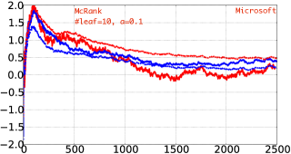
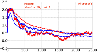
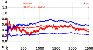
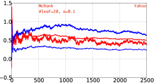
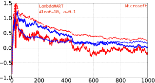
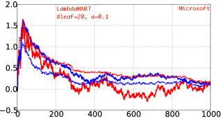
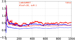
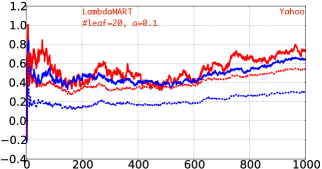
In table 2 and 3, for McRank and LambdaMART respectively, among 72 comparisons, OLE gains 68 and 56 improvements for at least over 0.1 point, and most of them are 0.3 to 0.4. These improvements are reasonable, as our baselines are strong, and in such large datasets. These statistics are based on six typical configurations, and demonstrate OLE is workable for the McRank and LambdaMART models in a general case.

We further analyze four measures separately, NDCG@(1, 3, 10) and ERR. Though both McRank (Figure 2, shown in the complementary material due to the space limit) and LambdaMART have been improved consistently with OLE, the NDCG@1 (real read line) and ERR (dotted blue line) have relatively smaller improvements. ERR is more difficult to improve than NDCG.

Improvements of NDCG@3 and NDCG@10 on McRank and LambdaMART are more robust in a variety of configurations. As NDCG@1 is computed on the first document predicted by models, and ERR is computed on the whole of ranking documents whose numbers are usually several dozens, in practice, the first page with 10 links returned by a search engine are more desired by users. So we think it may be more useful to improve NDCG@3 and NDCG@10 measures.

As OLE is supposed to have a faster convergence than SE, we also have a statistics of objective losses in the final iteration. OLE indeed leads to smaller objective losses, but not by that much, about 0.32% - 1%. As this work only focuses on the splitting rule in a single node, we also tried different strategies to generate node. Width-first search and depth-first search. Interestingly, depth-first search runs poorly for both baselines and our method. This is an open question and left to future exploration. We thus adopted the width-first search and limits the number of leaves.

Regarding the running time, there is no loss for the systems with derivative additive objective losses compared to SE in gradient boosting. Typical such systems are point-wise based. But for pair-wise and list-wise based, OLE suffers from extra overheads of maintaining exact second derivatives of objective loss function. In an incremental updating style, this overhead is about 30% of SE for pair-wise based, and regarding list-wise, there may be more.

5 Conclusion

In this paper, we propose a minimum objective loss based tree construction algorithm in the boosting framework, and analyze two existent tree construction principles, least square error and (robust) weighted square error. The former is widely used in the gradient boosting and practical learning to rank systems, while the latter is famous in LogitBoost and classification area. We successful build a relationship between our method and WSE in LogitBoost. We prove that WSE is just a special case of our method. This provides a theoretical support for (robust) LogitBoost and point-wise based ranking systems. Based on our analysis, we show MART is an ideal connection to SE, WSE, and OLE, and obtain a more concise formula for MART. Finally, for a full empirical comparison of the three principles, we implement two strong ranking systems, and examine them with a variety of configurations of regression trees in two largest public datasets. Our results indicate that our proposed method is better used for McRank, LambdaMART and MART systems.

References

- [1] Mokhtar S Bazaraa, Hanif D Sherali, and CM Shetty. Nonlinear Programming: Theory and Algorithms, 3rd Edition. John Wiley & Sons, 2006.
- [2] Chris Burges, Tal Shaked, Erin Renshaw, Ari Lazier, Matt Deeds, Nicole Hamilton, and Greg Hullender. Learning to rank using gradient descent. In ICML, pages 89–96, 2005.
- [3] Christopher JC Burges, Krysta Marie Svore, Paul N Bennett, Andrzej Pastusiak, and Qiang Wu. Learning to rank using an ensemble of lambda-gradient models. JMLR-Proceedings Track, pages 25–35, 2011.
- [4] Olivier Chapelle and Yi Chang. Yahoo! learning to rank challenge overview. JMLR-Proceedings Track, pages 1–24, 2011.
- [5] Olivier Chapelle and Mingrui Wu. Gradient descent optimization of smoothed information retrieval metrics. Information Retrieval, (3):216–235, 2010.
- [6] David Cossock and Tong Zhang. Subset ranking using regression. In COLT, pages 605–619. Springer, 2006.
- [7] Yoav Freund, Raj Iyer, Robert E Schapire, and Yoram Singer. An efficient boosting algorithm for combining preferences. JMLR, pages 933–969, 2003.
- [8] Jerome Friedman, Trevor Hastie, and Robert Tibshirani. additive logistic regression: A statistical view of boosting. Annals of statistics, 2000.
- [9] Jerome H Friedman. Greedy function approximation: a gradient boosting machine. Annals of Statistics, pages 1189–1232, 2001.
- [10] Tamir Hazan, Joseph Keshet, and David A Mcallester. Direct loss minimization for structured prediction. In NIPS, pages 1594–1602, 2010.
- [11] Quoc Le and Alexander Smola. Direct optimization of ranking measures. CoRR abs/0704.3359. Informal publication, 2007.
- [12] Ping Li. Abc-boost: adaptive base class boost for multi-class classification. In ICML, pages 625–632, 2009.
- [13] Ping Li. Fast abc-boost for multi-class classification. arXiv preprint arXiv:1006.5051, 2010.
- [14] Ping Li. Robust logitboost and adaptive base class (abc) logitboost. UAI, 2010.
- [15] Ping Li, Qiang Wu, and Christopher J Burges. Mcrank: Learning to rank using multiple classification and gradient boosting. In NIPS, pages 897–904, 2007.
- [16] Tie Yan Liu. Learning to rank for information retrieval. Foundations and Trends in IR, (3):225–331, 2009.
- [17] Robin L Plackett. The analysis of permutations. Applied Statistics, 1975.
- [18] Tao Qin, Tie Yan Liu, Jun Xu, and Hang Li. Letor: A benchmark collection for research on learning to rank for information retrieval. Information Retrieval, (4):346–374, 2010.
- [19] Pradeep D Ravikumar, Ambuj Tewari, and Eunho Yang. On ndcg consistency of listwise ranking methods. In AISTATS, pages 618–626, 2011.
- [20] Robert E Schapire and Yoav Freund. Boosting: Foundations and Algorithms. MIT Press, 2012.
- [21] Ming Tan, Tian Xia, Lily Guo, and Shao Jun Wang. Direct optimization of ranking measures for learning to rank models. In SIGKDD, pages 856–864, 2013.
- [22] Stephen Tyree, Kilian Q Weinberger, Kunal Agrawal, and Jennifer Paykin. Parallel boosted regression trees for web search ranking. In WWW, pages 387–396, 2011.
- [23] Hamed Valizadegan, Rong Jin, Ruofei Zhang, and Jianchang Mao. Learning to rank by optimizing ndcg measure. In NIPS, pages 1883–1891, 2009.
- [24] Qiang Wu, Christopher JC Burges, Krysta M Svore, and Jianfeng Gao. Adapting boosting for information retrieval measures. Information Retrieval, (3):254–270, 2010.
- [25] Fen Xia, Tie Yan Liu, and Hang Li. Statistical consistency of top-k ranking. In NIPS, pages 2098–2106, 2009.
- [26] Fen Xia, Tie Yan Liu, Jue Wang, Wensheng Zhang, and Hang Li. Listwise approach to learning to rank: theory and algorithm. In ICML, pages 1192–1199, 2008.