Estimator-Based Output-Feedback Stabilization of Linear Multi-Delay Systems using SOS

Abstract

In this paper, we investigate the estimator-based output feedback control problem of multi-delay systems. This work is an extension of recently developed operator-value LMI framework for infinite-dimensional time-delay systems. Based on the optimal convex state feedback controller and generalized Luenberger observer synthesis conditions we already have, the estimator-based output feedback controller is designed to contain the estimates of both the present state and history of the state. An output feedback controller synthesis condition is proposed using SOS method, which is expressed in a set of LMI/SDP constraints. The simulation examples are displayed to demonstrate the effectiveness and advantages of the proposed results.

I Introduction

Time delay widely exists in natural and engineered systems, often as a source of instability. Many works have been done on the study and control of time-delay systems during the last decades [1, 2], mainly focusing on stability analysis, such as [3] and [4]. Despite the considerable advances that have been made in the area of stability analysis, the problem of stabilization of time-delay systems has been relatively neglected [2, 5]. The primary problem in feedback stabilization of time-delay systems is the bilinearity between the controller and the Lyapunov certificate of stability. This bilinearity implies that combining parameterized controllers with standard approaches to Lyapunov-Krasovskii functional construction will result in Bilinear Matrix Inequalities – a problem for which no efficient optimization algorithms exist. Faced with this bilinearity, some papers use iterative methods to alternately optimize the Lyapunov functional and then the controller as in [6, 7]. However, this iterative approach is not guaranteed to converge. Recently, however, duality-based methods have been proposed within the SOS-based operator-theoretic framework – resulting in an LMI-based solution to the problem of $H_{\infty}$-optimal full-state-feedback control of multi-delay systems [8]. The primary disadvantage of the full-state feedback controllers proposed in [8] is that they assume accurate knowledge of all states of the system and moreover knowledge of the history of these states. Specifically, the controllers have the form

$$u(t)=K_{0}x(t)+\sum_{i}^{K}K_{1i}x(t-\tau_{i})+\sum_{i}^{K}\int_{-\tau_{i}}^{0}K_{2i}(s)x(t+s)ds$$ (1)

where the $H_{\infty}$-optimal controller gains $K_{0},K_{1i},K_{2i}$ are polynomials chosen to minimize the closed-loop $L_{2}$-gain bound $\gamma_{1}:=\text{sup}_{\omega\in L_{2}}\frac{\parallel z\parallel_{L_{2}}}{\parallel\omega\parallel_{L_{2}}}$. This formulation specifically precludes output-feedback controllers of the form $u(t)=Ky(t)$ or even $u(t)=Kx(t)$. In most practical cases such detailed measurements are not available.

The question of how to use measured outputs to reconstruct the full state is that of estimator design and is itself an area of active study (e.g. the Smith predictor can be thought of as an estimator using delayed output signals [10]). The $H_{\infty}$-optimal estimator design problem for multi-delay systems was itself directly addressed in the SOS-operator framework in [9], wherein the observer is a simulated PDE running parallel to the real system which corrects both the present states and the history of the states. This observer minimizes an $L_{2}$-gain bound on the effect of disturbances on a regulated error signal.

In this paper, we propose a framework for using controllers of the form in Eqn. (1) where the controller acts not on the full state, but the state estimate derived from a dynamic estimator constructed using the algorithm proposed in [9]. Specifically, the closed-loop dynamics have the form

$$\dot{x}(t)=A_{0}x(t)+\sum_{i}A_{i}x_{i}(t-\tau_{i})+B_{1}w(t)+B_{2}u(t)$$

$$\dot{\hat{x}}(t)=A_{0}\hat{x}(t)+\sum_{i}A_{i}\hat{\phi}_{i}(t,-\tau_{i})+L_{1}b_{0}(t)$$

$$\quad+\sum_{i}L_{2i}b_{i}(t,-\tau_{i})+\sum_{i}\int_{-\tau_{i}}^{0}L_{3i}(s)b_{i}(t,s)ds$$

$$\partial_{t}\hat{\phi}(t,s)=\partial_{s}\hat{\phi}(t,s)+L_{4}(s)b_{0}(t)+\sum_{j}L_{5ij}b_{j}(t,-\tau_{j})$$

$$\quad+L_{6i}(s)b_{i}(t,s)+\sum_{j}\int_{-\tau_{i}}^{0}L_{7ij}(s,\theta)b_{j}(t,\theta)d\theta$$

$$\hat{\phi}_{i}(t,0)=\hat{x}(t)\quad b_{i}(t,s)=C_{2}\hat{\phi}_{i}(t,s)-y(t+s)$$

$$b_{0}(t)=C_{2}\hat{x}(t)-y(t)$$

$$u(t)=K_{0}\hat{x}(t)+\sum_{i}K_{1i}\hat{x}(t-\tau_{i})+\sum_{i}\int_{-\tau_{i}}^{0}K_{2i}(s)\hat{x}(t+s)ds$$

$$y(t)=C_{2}x(t)+D_{2}w(t)$$

$$z(t)=C_{10}x(t)+\sum_{i}C_{1i}x_{i}(t-\tau_{i})+D_{1}w(t)$$

$$z_{e}(t)=C_{30}e(t)+\sum_{i}C_{3i}e_{i}(t,-\tau_{i})+D_{3}w(t)$$ (2)

where $x(t)\in\mathbb{R}^{n}$ is the state, $\hat{x}(t)\in\mathbb{R}^{n}$ is the estimate of state, $\hat{\phi}(t,s)\in\mathbb{R}^{n}$ is the estimate of history of state, $w\in L_{2}^{r}$ is an external disturbance input, $u(t)\in\mathbb{R}^{m}$ is the actuated input, $y(t)\in\mathbb{R}^{q}$ is the measured output, $z(t)\in\mathbb{R}^{p}$ is the regulated output, $z_{e}(t)\in\mathbb{R}^{p_{1}}$ is the estimated error of regulated output (not need to be $z(t)$ defined above). The delays $\tau_{i}>0$ for $i\in[1,\ldots,K]$ are ordered by increasing magnitude and $A_{0},A_{i},B_{1},B_{2},C_{10},C_{1i},C_{2},C_{30},C_{3i},D_{1},D_{2},D_{3}$ are constant matrices with appropriate dimensions. We assume $x(0)=\hat{x}(t)=0$ for all $s\in[-\tau_{K},0]$. The gains $K_{0},K_{1i},K_{2i}$ come from [8] and the gains $L_{0}$, $L_{1i}$, $L_{2i}$, $L_{3i}$, $L_{4i}$, $L_{5ij}$ come from [9]. By exploiting the properties of the gains and examining the dynamics of the closed-loop system, we show that the resulting dynamics are stable and establish a bound on the $H_{\infty}$-gain of the resulting closed-loop system. We furthermore propose a scheme for real-time numerical implementation of the observer-based controller and use numerical simulation to show that the resulting closed-loop system achieves internal stabilization.

I-A Notation

Shorthand notation used throughout this paper includes the Hilbert spaces $L_{2}^{m}[X]:=L_{2}(X;\mathbb{R}^{m})$ of square integrable functions from $X$ to $\mathbb{R}^{m}$ and $W_{2}^{m}[X]:=W^{1,2}(X;\mathbb{R}^{m})=H^{1}(X;\mathbb{R}^{m})=\{x:x,\dot{x}\in L_{2}^{m}[X]\}$. We use $L_{2}^{m},W_{2}^{m}$ when domains are clear from context. We also use the extensions $L_{2}^{n\times m}[X]:=L_{2}(X;\mathbb{R}^{n\times m})$ and $W_{2}^{n\times m}[X]:=W^{1,2}(X;\mathbb{R}^{n\times m})$ for matrix-valued functions. $S^{n}\subset\mathbb{R}^{n}\times n$ denotes the symmetric matrices. An operator $\mathcal{P}:Z\rightarrow Z$ is positive on a subset $X$ of Hilbert space $Z$ if $\left<x,\mathcal{P}x\right>\geq 0$ for all $x\in X$. $\mathcal{P}$ is coercive on $X$ if $\left<x,\mathcal{P}x\right>\geq\epsilon\lVert x\rVert^{2}_{Z}$ for some $\epsilon>0$ for all $x\in X$. Given an operator $\mathcal{P}:Z\rightarrow Z$ and a set $X\rightarrow Z$, we use the shorthand $\mathcal{P}(X)$ to denote the image of $\mathcal{P}$ on subset $X$. $I_{n}\in S^{n}$ denotes the identity matrix. $0_{n\times m}\in\mathbb{R}^{n\times m}$ is the matrix of zeros matrix with shorthand $0_{n}:=0_{n\times n}$. We will occasionally denote the intervals $T_{i}:=[-\tau_{i},0]$. For a natural number, $K\in N$, we adopt the index shorthand notation which denotes $[K]={1,\cdots,K}$. The symmetric completion of a matrix is denoted $*^{T}$.

II Previous Work on State Estimation and State-Feedback Control of DPS

In this section, we consider the a general class of distributed-parameter system (DPS) given as

$$\dot{\mathbf{x}}(t) =\mathcal{A}\mathbf{x}(t)+\mathcal{B}_{1}\omega(t)+\mathcal{B}_{2}u(t)\quad\mathbf{x}(0)=0$$

$$z(t) =\mathcal{C}_{1}\mathbf{x}(t)+\mathcal{D}_{1}\omega(t)$$

$$\mathbf{y}(t) =\mathcal{C}_{2}\mathbf{x}(t)+\mathcal{D}_{2}\omega(t)$$ (3)

where $\mathcal{A}:X\rightarrow Z$, $\mathcal{B}_{1}:\mathbb{R}\rightarrow Z$, $\mathcal{B}_{2}:U\rightarrow Z$, $\mathcal{C}_{1}:X\rightarrow\mathbb{R}$, $\mathcal{C}_{2}:X\rightarrow Y$, $\mathcal{D}_{1}:\mathbb{R}\rightarrow\mathbb{R}$ and $\mathcal{D}_{2}:\mathbb{R}\rightarrow Y$.

II-A Full State feedback controller design

Theorem 1

[8] Suppose $\mathcal{P}_{1}$ is a bounded, coercive linear operator $\mathcal{P}_{1}:X\rightarrow X$ with $\mathcal{P}_{1}(X)=X$ and which is self-adjoint with respect to the $Z$ inner product. Then $\mathcal{P}_{1}^{-1}$ exists; is bounded; is self-adjoint; $\mathcal{P}_{1}^{-1}:X\rightarrow X$; and $\mathcal{P}_{1}^{-1}$ is coercive.

Theorem 2

[8] Suppose there exists a scalar $\epsilon_{1}>0$, an operator $\mathcal{P}_{1}:Z\rightarrow Z$ which satisfies the conditions of Theorem 1, and an operator $\mathcal{H}:X\rightarrow U$ such that

$$\left<\mathcal{AP}_{1}\mathbf{h},\mathbf{h}\right>_{Z}+\left<\mathbf{h},\mathcal{AP}_{1}\mathbf{h}\right>_{Z}+\left<\mathcal{B}_{2}\mathcal{H}\mathbf{h},\mathbf{h}\right>_{Z}+\left<\mathbf{h},\mathcal{B}_{2}\mathcal{H}\mathbf{h}\right>_{Z}$$

$$+\left<\mathcal{B}_{1}\omega,\mathbf{h}\right>_{Z}+\left<\mathbf{h},\mathcal{B}_{1}\omega\right>_{Z}-\gamma_{1}\lVert\omega\rVert^{2}-\gamma_{1}\lVert\upsilon\rVert^{2}+\upsilon^{T}(\mathcal{C}_{1}\mathcal{P}\mathbf{h})$$

$$+(\mathcal{C}_{1}\mathcal{P}\mathbf{h})^{T}\upsilon+\upsilon^{T}(\mathcal{D}_{2}\mathcal{H}\mathbf{h})+(\mathcal{D}_{2}\mathcal{H}\mathbf{h})^{T}\upsilon+\upsilon^{T}(\mathcal{D}_{1}\omega)$$

$$+(D_{1}\omega)^{T}\upsilon\leq-\epsilon_{1}\lVert\mathbf{h}\rVert^{2}$$ (4)

for all $\mathbf{h}\in X$, $\omega\in\mathbb{R}^{r}$ and $\upsilon\in\mathbb{R}^{p}$. Then if $\omega$ and $z$ satisfy Eqn. (3) and $u(t)=\mathcal{K}\mathbf{x}(t)$ where $\mathcal{K}=\mathcal{HP}_{1}^{-1}$ we have $\lVert z\rVert_{L_{2}}\leq\gamma_{1}\lVert\omega\rVert_{L_{2}}$.

II-B Estimator design

In [9], a $H_{\infty}$ optimal estimator based on the traditional Luenberger structure is given for Eqn. (3), which can correct both the present states and history of the states and give a real-time estimate of the history of states. This estimator has the following dynamics

$$\dot{\hat{\mathbf{x}}}(t)=\mathcal{A}\hat{\mathbf{x}}(t)+\mathcal{L}(\mathcal{C}_{2}\hat{\mathbf{x}}(t)-\mathbf{\mathrm{y}}(t))$$ (5)

for a given operator $\mathcal{L}:Y\rightarrow Z$. By defining $\mathbf{e}(t)=\hat{\mathbf{x}}(t)-\mathbf{x}(t)$, one obtains the error dynamics as

$$\mathbf{\dot{e}}(t) =(\mathcal{A}+\mathcal{L}\mathcal{C}_{2})\mathbf{e}(t)-(\mathcal{B}_{1}+\mathcal{L}\mathcal{D}_{2})\omega(t)$$

$$z_{e}(t) =\mathcal{C}_{3}\mathbf{e}(t)+\mathcal{D}_{3}\omega(t)\quad\mathbf{e}(0)=0$$ (6)

where $\mathcal{C}_{3}:X\rightarrow\mathbb{R}$ and $\mathcal{D}_{3}:\mathbb{R}\rightarrow\mathbb{R}$.

Theorem 3

[9] Suppose there exist a scalar $\epsilon_{2}>0$ and bounded linear operators $\mathcal{P}_{2}:Z\rightarrow Z$ and $\mathcal{Z}:Y\rightarrow Z$ such that $\mathcal{P}_{2}$ is coercive and

$$\left<(\mathcal{P}_{2}\mathcal{A}+\mathcal{ZC}_{2})\mathbf{e},\mathbf{e}\right>_{Z}+\left<\mathbf{e},(\mathcal{P}_{2}\mathcal{A}+\mathcal{ZC}_{2})\mathbf{e}\right>_{Z}$$

$$-\left<\mathbf{e},(\mathcal{P}_{2}\mathcal{B}_{1}+\mathcal{ZD}_{2})\omega\right>_{Z}-\left<(\mathcal{P}_{2}\mathcal{B}_{1}+\mathcal{ZD}_{2})\omega,\mathbf{e}\right>_{Z}$$

$$-\gamma_{2}\lVert\omega\rVert^{2}-\gamma_{2}\lVert\upsilon_{e}\rVert^{2}+\left<\upsilon_{e},\mathcal{C}_{3}\mathbf{e}\right>+\left<\mathcal{C}_{3}\mathbf{e},\upsilon_{e}\right>$$

$$+\left<\upsilon_{e},\mathcal{D}_{3}\omega\right>+\left<\mathcal{D}_{3}\omega,\upsilon_{e}\right>\leq-\epsilon_{2}\lVert\mathbf{e}\rVert^{2}\quad$$ (7)

for all $\mathbf{e}\in X$, $\omega\in\mathbb{R}^{r}$ and $\upsilon_{e}\in\mathbb{R}^{p_{1}}$. Then $\mathcal{P}_{2}^{-1}$ is a bounded linear operator and for $\mathcal{L}=\mathcal{P}_{2}^{-1}\mathcal{Z}$, the solution of Eqn. (6) satisfies $\lVert z_{e}\rVert_{L_{2}}\leq\gamma_{2}\lVert\omega\rVert_{L_{2}}$.

III Main results

In this section, we give conditions under which the dynamics of the estimator-based controller is stable and give an expression for the $L_{2}$-gain of the closed-loop system. The conditions are given in abstract form. Later, in Theorem 6, we will given LMI-based sufficient conditions under which the conditions of Theorem 4 is satisfied.

III-A Estimator-Based Control for DPS

Combining Eqn. (3), Eqn. (5), and Eqn. (6) with $u(t)=\mathcal{K}\hat{\mathbf{x}}$, the closed-loop DPS dynamics are given as follows

$$\dot{\mathbf{x}}(t) =(\mathcal{A}+\mathcal{B}_{2}\mathcal{K})\mathbf{x}(t)+\mathcal{B}_{1}\omega(t)+\mathcal{B}_{2}\mathcal{K}\mathbf{e}(t)\quad$$

$$\mathbf{\dot{e}}(t) =(\mathcal{A}+\mathcal{L}\mathcal{C}_{2})\mathbf{e}(t)-(\mathcal{B}_{1}+\mathcal{L}\mathcal{D}_{2})\omega(t)$$

$$z(t) =\mathcal{C}_{1}\mathbf{x}(t)+\mathcal{D}_{1}\omega(t)$$

$$\mathbf{y}(t) =\mathcal{C}_{2}\mathbf{x}(t)+\mathcal{D}_{2}\omega(t)$$ (8)

$$z_{e}(t) =\mathcal{C}_{3}\mathbf{e}(t)+\mathcal{D}_{3}\omega(t)$$

where $\mathcal{K}:Z\rightarrow U$ and $\mathcal{L}:Y\rightarrow Z$. We assume $\mathbf{x}(0)=\mathbf{e}(0)=0$.

Theorem 4

Suppose there exist positive scalars $\epsilon_{1},\epsilon_{2}$, operators $\mathcal{H}:Z\rightarrow U$ and $\mathcal{P}_{1}:Z\rightarrow Z$ which satisfy the conditions of Theorem 1 with $\gamma_{1}$, and operators $\mathcal{P}_{2}:Z\rightarrow Z$, and $\mathcal{Z}:Y\rightarrow Z$ which satisfy Theorems 2 and 3 with $\gamma_{2}$. Then if there exists positive scalar $r$ such that

$$\left\langle\begin{bmatrix}\mathbf{h}\\ \mathbf{e}\end{bmatrix},\mathcal{M}\begin{bmatrix}\mathbf{h}\\ \mathbf{e}\end{bmatrix}\right\rangle\leq 0$$ (9)

for all $\mathbf{h},\mathbf{e}\in X$, where

$$\mathcal{M}=\left[\begin{array}[]{ccc}-\epsilon_{1}I&\mathcal{B}_{2}\mathcal{H}\mathcal{P}_{1}^{-1}\\ (\mathcal{B}_{2}\mathcal{H}\mathcal{P}_{1}^{-1})^{T}&-r\epsilon_{2}I\\ \end{array}\right].$$

Then for any $z(t)$, $z_{e}(t)$ and $w(t)$ which satisfy Eqn. (8) with $\mathcal{K}=\mathcal{HP}^{-1}$ and $\mathcal{L}=\mathcal{P}^{-1}\mathcal{Z}$, we have $\lVert z\rVert_{L_{2}}\leq\sqrt{\gamma_{1}(\gamma_{1}+r\gamma_{2})}\lVert\omega\rVert_{L_{2}}$ and $\lVert z_{e}\rVert_{L_{2}}\leq\gamma_{2}\lVert\omega\rVert_{L_{2}}$.

Proof:

Suppose $z(t)$, $z_{e}(t)$, $\mathbf{y}(t)$ $w(t)$, $\mathbf{e}(t)$, $\mathbf{x}(t)$ satisfy Eqn. (8). Since $z_{e}(t)$ is only affected by $\omega(t)$, we have by Theorem 3 that $\lVert z_{e}\rVert_{L_{2}}\leq\gamma_{2}\lVert\omega\rVert_{L_{2}}$. Define

$$V(t)=V_{1}(t)+rV_{2}(t)$$ (10)

where $V_{1}(t)=\left\langle\mathbf{x}(t),\mathcal{P}^{-1}\mathbf{x}(t)\right\rangle_{Z}$ and $V_{2}(t)=\left\langle\mathbf{e}(t),\mathcal{P}_{2}\mathbf{e}(t)\right\rangle_{Z}$. If we define expand $V_{2}(t)$ and apply Theorem 3, we have

$$\dot{V}_{2}(t) -\gamma_{2}\lVert\omega(t)\rVert^{2}\leq-\epsilon_{2}\lVert\mathbf{e}(t)\rVert^{2}.$$

If we define $\mathbf{h}(t)=\mathcal{P}_{1}^{-1}\mathbf{x}(t)\in X$ and differentiate $V_{1}(t)$, we have

$$\dot{V}_{1}(t)=\left<\mathcal{AP}_{1}\mathbf{h}(t),\mathbf{h}(t)\right>_{Z}+\left<\mathbf{h}(t),\mathcal{AP}_{1}\mathbf{h}(t)\right>_{Z}$$

$$+\left<\mathcal{B}_{2}\mathcal{H}\mathbf{h}(t),\mathbf{h}(t)\right>_{Z}+\left<\mathbf{h}(t),\mathcal{B}_{2}\mathcal{H}\mathbf{h}(t)\right>_{Z}$$

$$+\left<\mathcal{B}_{2}\mathcal{H}\mathcal{P}^{-1}_{1}\mathbf{e}(t),\mathbf{h}(t)\right>_{Z}+\left<\mathbf{h}(t),\mathcal{B}_{2}\mathcal{H}\mathcal{P}^{-1}_{1}\mathbf{e}(t)\right>_{Z}$$

$$\quad+\left<\mathcal{B}_{1}\omega(t),\mathbf{h}(t)\right>_{Z}+\left<\mathbf{h}(t),\mathcal{B}_{1}\omega(t)\right>_{Z}.$$

Applying Theorem 2, if we define $\upsilon(t)=\frac{1}{\gamma_{2}}z(t)$, one gets

$$\dot{V}_{1}(t)-\gamma_{1}\lVert\omega(t)\rVert^{2}+\gamma_{1}\lVert\upsilon(t)\rVert^{2}$$

$$\leq-\epsilon_{1}\lVert\mathbf{h}(t)\rVert^{2}+\left<\mathcal{B}_{2}\mathcal{H}\mathcal{P}^{-1}_{1}\mathbf{e}(t),\mathbf{h}(t)\right>_{Z}$$

$$+\left<\mathbf{h}(t),\mathcal{B}_{2}\mathcal{H}\mathcal{P}^{-1}_{1}\mathbf{e}(t)\right>_{Z}.$$

Combining the results above, we have

$$\dot{V}(t) -(\gamma_{1}+r\gamma_{2})\lVert\omega(t)\rVert^{2}+\gamma_{1}\lVert\upsilon(t)\rVert^{2}$$

$$\leq-\epsilon_{1}\lVert\mathbf{h}(t)\rVert^{2}-r\epsilon_{2}\lVert\mathbf{e}(t)\rVert^{2}$$

$$+\left<\mathcal{B}_{2}\mathcal{H}\mathcal{P}^{-1}_{1}\mathbf{e}(t),\mathbf{h}(t)\right>_{Z}+\left<\mathbf{h}(t),\mathcal{B}_{2}\mathcal{H}\mathcal{P}^{-1}_{1}\mathbf{e}(t)\right>_{Z}$$

$$=\left\langle\begin{bmatrix}\mathbf{h}(t)\\ \mathbf{e}(t)\end{bmatrix},\mathcal{M}\begin{bmatrix}\mathbf{h}(t)\\ \mathbf{e}(t)\end{bmatrix}\right\rangle.$$

Then if there exist a positive scalar $r$ such that Eqn. (9) is satisfied, it follows

$$\dot{V}(t)-(\gamma_{1}+r\gamma_{2})\lVert\omega(t)\rVert^{2}+\gamma_{1}\lVert\upsilon(t)\rVert^{2} \leq 0.$$

Integrating in time and using $V(0)=0$, we have

$$\lVert z\rVert_{L_{2}} \leq\sqrt{\gamma_{1}(\gamma_{1}+r\gamma_{2})}\lVert\omega\rVert_{L_{2}}.$$

The proof is completed. ∎

III-B Expressing Multi-delay system into DPS

In this section, we apply Theorem 4 to the case of multi-delay systems. Specifically, we consider solutions to the system of equations given by Eqn. (2).

Firstly, considering $e(t)=\hat{x}(t)-x(t)$, we write Eqn. (2) into the form in Eqn. (3). Following the mathematical formalism developed in [2], define the inner-product space $Z_{m,n,K}$:=$\{\mathbb{R}^{m}\times$ $L_{2}^{n}[-\tau_{1},0]\times\cdots\times L_{2}^{n}[-\tau_{K},0]\}$ and for $\{x,\phi_{1},\cdots,\phi_{K}\}\in Z_{m,n,K}$, we use the following notation

$$\begin{bmatrix}x\\ \phi_{i}\end{bmatrix}:=\{x,\phi_{1},\cdots,\phi_{K}\}$$

and we define the inner product on $Z_{m,n,K}$ as

$$\left<\begin{bmatrix}y\\ \psi_{i}\end{bmatrix},\begin{bmatrix}x\\ \phi_{i}\end{bmatrix}\right>_{Z_{m,n,K}}=\tau_{K}y^{T}x+\sum_{i=1}^{K}\int_{-\tau_{i}}^{0}\psi_{i}(s)^{T}\phi_{i}(s)ds.$$

We simplify the notation $Z_{m,n,k}$ when $m=n$ as $Z_{n,k}$.
Then the state-space for system (8) is defined as

$$X:=\left\{\begin{bmatrix}x\\ \phi_{i}\end{bmatrix}\in\mathcal{Z}_{n,K}:\begin{array}[]{c}\phi_{i}\in W_{2}^{n}[-\tau_{i},0]\text{ and }\phi_{i}(0)=x\\ \text{ for all }i\in[K]\end{array}\right\}.$$

We now represent the infinitesimal generator, $\mathcal{A}:X\rightarrow Z_{n,K}$ of Eqn. (8) as

$$\mathcal{A}\begin{bmatrix}x\\ \phi_{i}\end{bmatrix}(s) =\begin{bmatrix}A_{0}x(t)+\sum A_{i}\phi_{i}(-\tau_{i})\\ \dot{\phi_{i}}(s)\end{bmatrix}.$$

Furthermore, $\mathcal{B}_{1}:\mathbb{R}^{r}\rightarrow Z_{n,K}$, $\mathcal{B}_{2}:\mathbb{R}^{m}\rightarrow Z_{n,K}$, $\mathcal{C}_{1}:Z_{n,K}\rightarrow\mathbb{R}^{p}$, $\mathcal{C}_{2}:X\rightarrow Z_{q,K}$, $\mathcal{C}_{3}:Z_{n,K}\rightarrow\mathbb{R}^{p_{1}}$, $\mathcal{D}_{1}:\mathbb{R}^{r}\rightarrow\mathbb{R}^{p}$, $\mathcal{D}_{3}:\mathbb{R}^{r}\rightarrow Z^{p_{1}}$ are defined as

$$\mathcal{B}_{1}\omega(t) :=\begin{bmatrix}B_{1}\omega(t)\\ 0\end{bmatrix}\quad\mathcal{B}_{2}u(t):=\begin{bmatrix}B_{2}u(t)\\ \ 0\end{bmatrix}$$

$$\mathcal{C}_{j}\begin{bmatrix}x\\ \phi_{i}\end{bmatrix}(s) :=C_{j0}x(t)+\sum_{i}C_{ji}\phi_{i}(-\tau_{i})\quad j=1,3$$

$$\mathcal{C}_{2}\begin{bmatrix}x\\ \phi_{i}\end{bmatrix}(s) :=\begin{bmatrix}C_{2}x(t)\\ C_{2}\phi_{i}(s)\end{bmatrix}$$ (11)

$$\mathcal{D}_{j}\omega(t) :=D_{j}\omega(t)\quad j=1,3.$$

Here we assume $\mathcal{D}_{2}=0$. Note for any solution $x(t)$ of Eqn. (2), using the above notation

$$(\mathbf{x}(t))(s)=\left[\begin{array}[]{c}x(t)\\ x(t+s)\end{array}\right],$$

then $\mathbf{x}(t)$ satisfies Eqn. (8). The converse statement is also true. The same is true for $\mathbf{e}(t)$, $\mathbf{y}(t)$.

III-C The operators framework

A class of operators $\mathcal{P}_{\{P,Q_{i},S_{i},R_{ij}\}}:Z_{m,n,K}\rightarrow Z_{m,n,K}$ is introduced which is parameterized by matrix $P$ and matrix-valued functions $Q_{i}\in W_{2}^{m\times n}[-\tau_{i},0]$, $S_{i}\in W_{2}^{n\times n}[-\tau_{i},0]$, $R_{ij}\in W_{2}^{n\times n}[-\tau_{i},0]\times[-\tau_{j},0]$ as

$$\left(\mathcal{P}_{\{P,Q_{i},S_{i},R_{ij}\}}\begin{bmatrix}x\\ \phi_{i}\end{bmatrix}\right)(s):=$$ (12)

$$\begin{bmatrix}Px+\sum_{i}^{K}\int_{-\tau_{i}}^{0}Q_{i}(s)\phi_{i}(s)ds\\ \tau_{K}Q^{T}_{i}(s)+\tau_{K}S_{i}(s)\phi_{i}(s)+\sum_{i}^{K}\int_{-\tau_{j}}^{0}R_{ij}(s,\theta)\phi_{j}(\theta)d\theta\end{bmatrix}.$$

Lemma 5

[8] Suppose that $P\in\mathbb{R}^{n\times n}$, $S_{i}\in W_{2}^{n\times n}[T_{i}]$, $R_{ij}\in W_{2}^{n\times n}[T_{i}\times T_{j}]$ satisfying $S_{i}(s)=S_{i}^{T}(s)$, $R_{ij}(s,\theta)=R_{ji}^{T}(\theta,s)$, $P=\tau_{K}Q_{i}^{T}(0)$ and $Q_{j}(s)=R_{ij}(0,s)$ for all $i,j\in[K]$. Moreover suppose $\mathcal{P}_{\{P,Q_{i},S_{i},R_{ij}\}}$ is coercive on $Z_{n,K}$. Then $\mathcal{P}_{\{P,Q_{i},S_{i},R_{ij}\}}$ is a self-adjoint bounded linear operator with respect to the inner product defined on $Z_{n,K}$; $\mathcal{P}:X\rightarrow X$; and $\mathcal{P}_{\{P,Q_{i},S_{i},R_{ij}\}}(X)=X$.

Now let us turn to the operators used in Theorem 4. We define $\mathcal{P}_{1}:=\mathcal{P}_{\{P_{1},Q_{1i},S_{1i},R_{1ij}\}}$ and $\mathcal{P}_{2}:=\mathcal{P}_{\{P_{2},Q_{2i},S_{2i},R_{2ij}\}}$ and we parameterize the decision variable $\mathcal{H}:Z_{n,k}\rightarrow\mathbb{R}^{m}$ using matrices $H_{0},H_{1i}$ and functions $H_{2i}$ as

$$\mathcal{H}\begin{bmatrix}y\\ y_{i}\end{bmatrix}(s)=\left[H_{0}y+\sum_{i}H_{1i}y_{i}(-\tau_{i})+\sum_{i}\int_{-\tau_{i}}^{0}H_{2i}(s)y_{i}(s)ds\right].$$ (13)

Similarly, the decision variable $\mathcal{Z}$ is parameterized as

$$\mathcal{Z}\begin{bmatrix}y\\ y_{i}\end{bmatrix}(s) =\begin{bmatrix}Z_{1}y_{0}+\sum_{i}Z_{2i}y_{i}(-\tau_{i})+\sum_{i}\int_{-\tau_{i}}^{0}Z_{3i}(s)y_{i}(s)ds\\ \tau_{K}z_{i}(s)\end{bmatrix}$$

$$z_{i}(s) =Z_{4i}(s)y_{0}+\sum_{j}Z_{5ij}(s)y_{j}(-\tau_{j})+Z_{6i}(s)y_{i}(s)$$

$$+\sum_{j}\int_{-\tau_{j}}^{0}Z_{7ij}(s,\theta)y_{j}(\theta)d\theta.$$ (14)

In [9], it was shown that for $\mathcal{Z}$ as parameterized above, if $\mathcal{L}=\mathcal{P}^{-1}_{1}\mathcal{Z}$, then the error injection operator $\mathcal{L}:Z_{q,k}\rightarrow Z_{n,k}$ corresponds to the estimator structure defined in Eqn. (2). The same is true for $\mathcal{K}=\mathcal{H}\mathcal{P}_{2}^{-1}$.

To simplify presentation, we do not present the LMI constraints on the coefficients of $\{P,Q_{i},S_{i},R_{ij}\}$ which ensure $\mathcal{P}_{\{P,Q_{i},S_{i},R_{ij}\}}\geq 0$. Rather, we simply represent these constraints using the following notation.

$$\Xi_{d,m,n,K}:=$$

$$\left\{\{P,Q_{i},R_{ij},S_{i}\}:\begin{subarray}{c}\{P,Q_{i},R_{ij},S_{i}\}\text{ satisfy the conditions of Corollary 4}\\ \text{in~{}\cite[cite]{[\@@bibref{}{b12}{}{}]}}\end{subarray}\right\}.$$

By Theorem 8 in [8], if $\{P-\epsilon I,Q_{i},R_{ij},S_{i}-\epsilon I\}\in\Xi_{d,m,n,K}$, then $\mathcal{P}_{\{P,Q_{i},S_{i},R_{ij}\}}$ is coercive and has an inverse of the form $\hat{\mathcal{P}}:=\hat{\mathcal{P}}_{\{\hat{P},\frac{1}{\tau_{K}}\hat{Q}_{i},\frac{1}{\tau_{K}^{2}}\hat{S}_{i},\frac{1}{\tau_{K}}\hat{R}_{ij}\}}$. In this paper, we do not explicitly represent the map to $\{\hat{P},\hat{Q}_{i},\hat{S}_{i},\hat{R}_{ij}\}$, but rather combine it into a single map from $\{P,Q_{i},S_{i},R_{ij}\}$ and $\{Z_{1},Z_{2i},Z_{3i},Z_{4i},Z_{5ij},Z_{6i},Z_{7ij}\}$ (resp. $\{H_{1},H_{2i},H_{3i}\}$) to $\{L_{1},L_{2i},L_{3i},L_{4i},L_{5ij},L_{6i},L_{7ij}\}$ (resp. $\{K_{0},K_{1i},K_{2i}\}$) which we then denote using the following.

Definition of $\mathcal{L}_{o}$:

$$\{L_{1},L_{2i},\cdots,L_{7ij}\}=\mathcal{L}_{o}(\{P,Q_{i},S_{i},R_{ij}\},\{Z_{1},Z_{2},\cdots,Z_{7ij}\})$$

to indicate that if $\{\hat{P},\hat{Q}_{i},\hat{S}_{i},\hat{R}_{ij}\}$ are as defined in Theorem 8 in [8], then $\{L_{1},L_{2i},\cdots,L_{7ij}\}$, $\{\hat{P},\hat{Q}_{i},\hat{S}_{i},\hat{R}_{ij}\}$, and $\{Z_{1},Z_{2},\cdots,Z_{7ij}\}$ satisfy Lemma 7 in [9].

Definition of $\mathcal{L}_{c}$: Likewise, we say

$$\{K_{0},K_{1i},K_{2i}\}=\mathcal{L}_{c}(\{P,Q_{i},S_{i},R_{ij}\},\{H_{0},H_{1i},H_{2i}\})$$

to indicate that if $\{\hat{P},\hat{Q}_{i},\hat{S}_{i},\hat{R}_{ij}\}$ are as defined in Theorem 8 in [8], then $\{K_{0},K_{1i},K_{2i}\}$, $\{\hat{P},\hat{Q}_{i},\hat{S}_{i},\hat{R}_{ij}\}$, and $\{H_{0},H_{1i},H_{2i}\}$ satisfy Lemma 9 in [8].

III-D Theorem 4 applied to Multi-delay systems

In this section, we formulate the conditions of Theorem 4 into multi-delay systems as a linear operator inequality where all operators are the form of Eqn. (12).

Theorem 6

Suppose there exist $d\in\mathbb{N}$, positive scalars $\epsilon,\epsilon_{1},\epsilon_{2}$, $\gamma_{1},\gamma_{2}$, $\{P_{1},Q_{1i},S_{1i},R_{1ij}\}$ satisfying Lemma 5, matrices $P_{2}\in\mathbb{R}^{n\times n}$, polynomials $S_{2i},Q_{2i}\in W_{2}^{n\times n}[T_{i}]$, $R_{2ij}\in W_{2}^{n\times n}[T_{i}\times T_{j}]$, matrices $H_{0},H_{1i}\in\mathbb{R}^{p\times n}$, polynomial $H_{2i}\in W_{2}^{p\times n}[T_{i}]$, matrices $Z_{1},Z_{2i}\in\mathbb{R}^{n\times q}$, polynomials $Z_{3i}$, $Z_{4i}$, $Z_{5ij}$, $Z_{6i}\in W_{2}^{n\times q}[T_{i}]$ and $Z_{7ij}\in W_{2}^{n\times q}[T_{i}\times T_{j}]$ for all $i$, $j\in[K]$ such that

$$\{P_{1}-\epsilon I,Q_{1i},S_{1i},R_{1ij}\} \in\Xi_{d,n,n,K}$$

$$-\{E_{1}+\epsilon_{1}\hat{I}_{1},F_{1i},N_{1i}+\epsilon_{1}I,G_{1ij}\} \in\Xi_{d,m_{0},n,K}$$

$$\{P_{2}-\epsilon I,Q_{2i},S_{2i},R_{2ij}\} \in\Xi_{d,n,n,K}$$

$$-\{E_{2}+\epsilon_{2}\hat{I}_{2},F_{2i},N_{2i}+\epsilon_{2}I,G_{2ij}\} \in\Xi_{d,m_{1},n,K}$$

where

$$\{E_{1},F_{1i},{H}_{1i},G_{1ij}\}$$

$$\qquad=\mathcal{L}_{1}(\{P_{1},Q_{1i},S_{1i},R_{1ij}\},\{H_{0},H_{1i},H_{2i}\})$$

$$\{E_{2},F_{2i},{H}_{2i},G_{2ij}\}$$

$$\qquad=\mathcal{L}_{2}(\{P_{1},Q_{2i},S_{2i},R_{2ij}\},\{Z_{0},Z_{1i},Z_{2i},\cdots,\})$$

and $m_{0}=p+r+n(K+1)$, $m_{1}=p+r+n(K+1)$, $\mathcal{L}_{1}$ and $\mathcal{L}_{2}$ are as defined in Appendix, $\hat{I}_{1}=\text{diag}(0_{r+p},I_{n},0_{nK})$ and $\hat{I}_{2}=\text{diag}(0_{r+p_{1}},I_{n},0_{nK})$.

Let

$$\{L_{1},L_{2i},\cdots,L_{7ij}\}=\mathcal{L}_{o}(\{P,Q_{i},S_{i},R_{ij}\},\{Z_{1},Z_{2},\cdots,Z_{7ij}\})$$

and

$$\{K_{0},K_{1i},K_{2i}\}=\mathcal{L}_{c}(\{P,Q_{i},S_{i},R_{ij}\},\{H_{0},H_{1i},H_{2i}\}).$$

Now further suppose that $r>0$ and

$$-\{E_{3}+\epsilon_{3}\hat{I}_{3},F_{3i},N_{3i},0\} \in\Xi_{d,n(K+2),2n,K}$$ (15)

where

$$E_{3}=\begin{bmatrix}-\frac{\epsilon_{1}}{\tau_{K}}I&B_{2}K_{0}&B_{2}K_{11}&\ldots&B_{2}K_{1k}\\ *^{T}&-r\frac{\epsilon_{2}}{\tau_{K}}I&0&\ldots&0\\ *^{T}&*^{T}&0&\ldots&0\\ \vdots&\vdots&\vdots&\ddots&\vdots\\ *^{T}&*^{T}&*^{T}&*^{T}&0\end{bmatrix}$$

$$F_{3i}=\begin{bmatrix}K^{T}_{2i}(s)B^{T}_{2}&0&0&\cdots&0\\ 0&0&0&\cdots&0\end{bmatrix}^{T}\quad$$

$$N_{3i}=\begin{bmatrix}-r\frac{\epsilon_{2}}{\tau_{K}}I&0\\ 0&-\epsilon_{1}I\end{bmatrix}.$$

and $\hat{I}_{3}=\text{diag}(I_{n},0_{n},0_{nK})$. Then if $w$, $z$ and $z_{e}$ satisfy Eqn. (2) for some $\mathbf{x}$ and $\hat{\mathbf{x}}$, we have $\lVert z\rVert_{L_{2}}\leq\sqrt{\gamma_{1}(\gamma_{1}+r\gamma_{2})}\lVert\omega\rVert_{L_{2}}$ and $\lVert z_{e}\rVert_{L_{2}}\leq\gamma_{2}\lVert\omega\rVert_{L_{2}}$.

Proof:

Let $\mathcal{A},\mathcal{B}_{1},\mathcal{B}_{2},\mathcal{C}_{1},\mathcal{D}_{1},\mathcal{C}_{2},\mathcal{D}_{2}$ be as defined in Eqn. (11). Now define $\mathcal{L}$ as

$$\mathcal{L}\begin{bmatrix}y_{0}\\ y_{i}\end{bmatrix}(s)=\begin{bmatrix}L_{1}y_{0}+\sum_{i}L_{2i}y_{i}(-\tau_{i})+\sum_{i}\int_{-\tau_{i}}^{0}L_{3i}(s)y_{i}(s)ds\\ l_{i}(s)\end{bmatrix}$$

$$l_{i}(s)=L_{4i}(s)y_{0}+\sum_{j}L_{5ij}(s)y_{j}(-\tau_{j})+L_{6i}(s)y_{i}(s)$$

$$\qquad+\sum_{j}\int_{-\tau_{j}}^{0}L_{7ij}(s,\theta)y_{j}(\theta)d\theta.$$ (16)

and $\mathcal{K}$ as

$$u(t) =\mathcal{K}\mathbf{x}(t)$$ (17)

$$=K_{0}x(t)+\sum_{i}K_{1i}x(t-\tau_{i})+\sum_{i}\int_{-\tau_{i}}^{0}K_{2i}(s)x(t+s)ds.$$

Since $\{P_{1}-\epsilon I,Q_{1i},S_{1i}-\epsilon I,R_{1ij}\}\in\Xi_{d,n,n,K}$ and $\{P_{2}-\epsilon I,Q_{2i}-\epsilon I,S_{2i},R_{2ij}\}\in\Xi_{d,n,n,K}$, $\mathcal{P}_{1}:=\mathcal{P}_{\{P_{1},Q_{1i},S_{1i},R_{1ij}\}}$ and $\mathcal{P}_{2}:=\mathcal{P}_{\{P_{2},Q_{2i},S_{2i},R_{2ij}\}}$ are coercive. Let $\mathcal{Z}$ be as defined in (14) and $\mathcal{H}$ be as defined in (13). Now by Theorem 5 and Lemma 10 in [8], $\mathcal{K}=\mathcal{H}\mathcal{P}_{1}^{-1}$ and by Theorem 5 and Lemma 9 in [9], $\mathcal{L}=\mathcal{P}_{1}^{-1}\mathcal{Z}$.

Next, if we define

$$\mathcal{M}=\left[\begin{array}[]{ccc}-\epsilon_{1}I&\mathcal{B}_{2}\mathcal{H}\mathcal{P}_{1}^{-1}\\ (\mathcal{B}_{2}\mathcal{H}\mathcal{P}_{1}^{-1})^{*}&-r\epsilon_{2}I\\ \end{array}\right]=\begin{bmatrix}-\epsilon_{1}I&\mathcal{B}_{2}\mathcal{K}\\ (\mathcal{B}_{2}\mathcal{K})^{*}&-r\epsilon_{2}I\end{bmatrix}$$

and for $\mathbf{h},\mathbf{e}\in X$, we expand the expression

$$\left\langle\begin{bmatrix}\mathbf{h}\\ \mathbf{e}\end{bmatrix},\mathcal{M}\begin{bmatrix}\mathbf{h}\\ \mathbf{e}\end{bmatrix}\right\rangle$$

$$=\left\langle\mathcal{B}_{2}\mathcal{K}\mathbf{e},\mathbf{h}\right\rangle+\left\langle\mathbf{h},\mathcal{B}_{2}\mathcal{K}\mathbf{e}\right\rangle_{Z}-\epsilon_{1}\left\lVert{\mathbf{h}}\right\rVert^{2}-r\epsilon_{2}\left\lVert{\mathbf{e}}\right\rVert^{2}$$

Now let

$$\mathbf{h}(s)=\begin{bmatrix}h_{1}\\ h_{2i}(s)\end{bmatrix},\mathbf{e}(s)=\begin{bmatrix}e_{1}\\ e_{2i}(s)\end{bmatrix}$$

We have

$$\left\langle\begin{bmatrix}\mathbf{h}\\ \mathbf{e}\end{bmatrix},\mathcal{M}\begin{bmatrix}\mathbf{h}\\ \mathbf{e}\end{bmatrix}\right\rangle$$

$$=2\tau_{K}h_{1}^{T}(B_{2}K_{0}e_{1}+\sum_{i}B_{2}K_{1i}e_{2i}(-\tau_{i})$$

$$+\sum_{i}\int_{-\tau_{K}}^{0}B_{2}K_{2i}e_{2i}(s)ds)-\epsilon_{1}h_{1}^{T}h_{1}-r\epsilon_{2}e_{1}^{T}e_{1}$$

$$-\epsilon_{1}\sum_{i}\int_{-\tau_{K}}^{0}h_{2i}^{T}(s)h_{2i}(s)ds-r\epsilon_{2}\sum_{i}\int_{-\tau_{K}}^{0}e_{2i}^{T}(s)e_{2i}(s)ds.$$

If we define $f_{1}=[h_{1}^{T},e^{T}_{1},e^{T}_{2i}(-\tau_{1}),\cdots,e^{T}_{2}(-\tau_{K})^{T}]^{T}$ and $f_{2i}(s)=[e_{2i}^{T}(s),h_{2i}^{T}(s)]^{T}$, then we obtain

$$\left\langle\begin{bmatrix}\mathbf{h}\\ \mathbf{e}\end{bmatrix},\mathcal{M}\begin{bmatrix}\mathbf{h}\\ \mathbf{e}\end{bmatrix}\right\rangle$$

$$=\left\langle\begin{bmatrix}f_{1}\\ f_{2}i(s)\end{bmatrix},\mathcal{P}_{\{E_{3},F_{3i},N_{3i},0\}}\begin{bmatrix}f_{1}\\ f_{2i}(s)\end{bmatrix}\right\rangle_{Z_{n(K+2),2n,K}}.$$

Since $-\{E_{3}+\epsilon_{3}\hat{I}_{3},F_{3i},N_{3i},0\}\in\Xi_{d,n(K+2),2n,K}$, we conclude that $\mathcal{M}\leq 0$ and hence all the conditions of Theorem 4 are satisfied. Finally, suppose that $y(t)$, $z(t)$, $z_{e}(t)$, and $x(t)$ satisfy Eqn. (2). If we define $\mathbf{y}=y$, and

$$(\mathbf{x}(t))(s)=\left[\begin{array}[]{c}x(t)\\ x(t+s)\end{array}\right],\;(\mathbf{e}(t))(s)=\begin{bmatrix}\hat{x}(t)-x(t)\\ \hat{x}(t+s)-x(t+s)\end{bmatrix},$$

then $\omega(t)$ $y(t)$, $z(t)$, $z_{e}(t)$, $\mathbf{e}(t)$ and $\mathbf{x}(t)$ satisfy (8) and hence by Theorem 4, we have that $\left\lVert{z}\right\rVert\leq\sqrt{\gamma_{1}(\gamma_{1}+r\gamma_{2})}\left\lVert{\omega}\right\rVert$ and $\left\lVert{z_{e}}\right\rVert_{L_{2}}\leq\gamma_{2}\left\lVert{\omega}\right\rVert_{L_{2}}$. ∎

Theorem 7 provides a method for using LMIs to construct estimator-based output feedback controllers for systems with multiple delays, including a bound on the closed loop $L_{2}$-gain.

IV Numerical implementation, testing, validation

The algorithms described in this paper have been implemented in Matlab within the DelayTOOLs framework, which is based on SOSTOOLS and the pvar framework. All the tools needed are available online for validation or download on Code Ocean [3].

For simulation, a fixed-step forward-difference-based discretization method is used, with a different set of states representing each delay channel. In the simulation results given below, 20 spatial discretization points are used for each delay channel.

IV-A Example 1

In this example, we consider the unstable system modified from the result in [12] which is in the form of Eqn. (2) with

$$A_{0}=\left[\begin{matrix}0&0\\ 0&1\end{matrix}\right]\quad A_{1}=\left[\begin{matrix}-1&-1\\ 0&-0.9\end{matrix}\right]\quad B_{1}=\left[\begin{matrix}1&0\\ 0&1\end{matrix}\right]$$

$$B_{2}=\left[\begin{matrix}0\\ 1\end{matrix}\right]\quad C_{10}=\left[\begin{matrix}1&0\end{matrix}\right]\quad D_{1}=\left[\begin{matrix}1&0\end{matrix}\right]$$

$$C_{30}=\left[\begin{matrix}1.5&0.5\end{matrix}\right]\quad D_{3}=\left[\begin{matrix}1&0\end{matrix}\right]\quad C_{2}=\left[\begin{matrix}1&0\end{matrix}\right]$$

and $\tau=0.99$.

IV-B Example 2

This example is given by modifying the result from [10] which is in the form of Eqn. (2) with

$$A_{0}=\left[\begin{matrix}-10&10\\ 0&1\end{matrix}\right]\quad A_{1}=\left[\begin{matrix}1&1\\ 1&1\end{matrix}\right]\quad B_{1}=\left[\begin{matrix}1&0\\ 0&1\end{matrix}\right]$$

$$B_{2}=\left[\begin{matrix}1\\ 1\end{matrix}\right]u(t)\quad C_{10}=\left[\begin{matrix}1&0\\ 0&1\end{matrix}\right]\quad C_{30}=\left[\begin{matrix}1.2&0\\ 0&1.2\end{matrix}\right]$$

$$C_{2}=\left[\begin{matrix}0&10\end{matrix}\right]\quad\text{and}\quad\tau=0.3.$$

IV-C Example 3

This example considers the 2-delay case as a modified version of Example 1, which is in the form of Eqn. (2) with

$$A_{0}=\left[\begin{matrix}0&0\\ 0&1\end{matrix}\right]\quad A_{i}=\left[\begin{matrix}-0.5&-0.5\\ 0&-0.45\end{matrix}\right]\quad i=1,2$$

$$B_{1}=\left[\begin{matrix}1&0&0\\ 0&1&0\end{matrix}\right]\quad B_{2}=\left[\begin{matrix}1\\ 1\end{matrix}\right]\quad C_{10}=\left[\begin{matrix}1&0\end{matrix}\right]$$

$$C_{30}=\left[\begin{matrix}1.1&0.2\end{matrix}\right]\quad C_{2}=\left[\begin{matrix}0&1\end{matrix}\right]$$

and $\tau_{1}=0.5,\tau_{2}=1$.

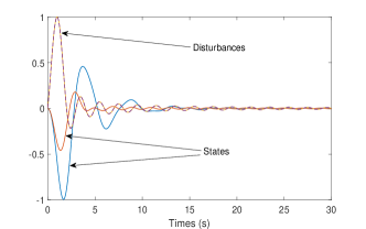
Figure 1: Errors in the estimated state $e(t)$ in closed-loop response for a sinc disturbance for Example 1

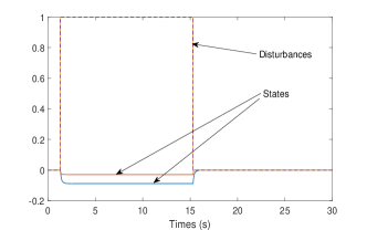
Figure 2: Errors in the estimated state $e(t)$ in closed-loop response for a step-like disturbance for Example 2

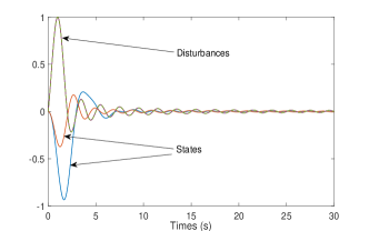
Figure 3: Errors in the estimated state $e(t)$ in closed-loop response for a sinc disturbance for Example 3

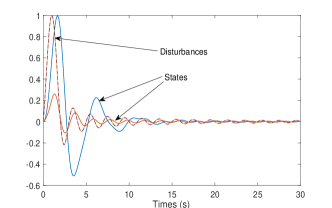
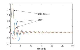
Figure 4: State trajectory $x(t)$ in closed-loop response for a sinc disturbance for Example 1

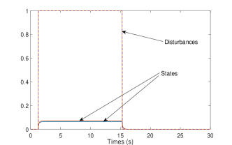
Figure 5: State trajectory $x(t)$ in closed-loop response for a step-like disturbance for Example 2

Figure 6: State trajectory $x(t)$ in closed-loop response for a sinc disturbance for Example 3

These three numerical examples are used to validate and test the accuracy of the algorithm defined in Theorem 6. In each instance, we find a state feedback controller, an observer, and construct observer-based controller. In Table I, we find the $\gamma_{1},\gamma_{2}$ obtained from Theorem 7 as compared to an H_∞ optimal output feedback controller obtained by using a 10th order Pad$\acute{\text{e}}$ approximation of the delay terms in Table 1. We also give a lower bound on the real $L_{2}$ gain $\gamma_{\text{real}}$ by numerically simulating the effect of a disturbance $\omega(t)$ on the $L_{2}$-norm of the regulated output $z(t)$ and comparing to the $L_{2}$-norm of the input. The closed-loop dynamics are validated in Figs. 1-6 where we see the estimator-based controller is effective in stabilization of systems that are open-loop unstable.

V Conclusion

In this paper, we have proposed a method for designing estimator-based output feedback controllers for systems with multiple delays. This approach combines an $H_{\infty}$-optimal estimator with an $H_{\infty}$-optimal full-state feedback controller and proves a bound on the $L_{2}$-norm of the resulting dynamics. These controllers are applicable to systems with multiple known delays and consider process noise, but not sensor noise. Furthermore, we have developed an efficient numerical implementation of the observer-based controller and have posted this implementation online. Numerical examples indicate that the $L_{2}$-gain of the resulting estimator-based controllers is relatively close to, but does not exactly achieve the minimum possible closed-loop $L_{2}$-gain as estimated using a Padé approximation.

	Example 1			Example 2			Example 3
	d=1	d=2	d=4	d=1	d=2	d=4	d=1	d=2	d=4
$\gamma_{1\text{min}}$	1.9082	1.6829	1.6359	0.1067	0.1060	0.1059	1.049	0.9892	0.9596
$\gamma_{2\text{min}}$	4.1485	4.1425	4.1425	0.1325	0.1325	0.1325	1.4862	1.4851	1.4851
$\gamma_{\text{min}}$	3.0450			0.1104			1.3499
$\gamma_{\text{real}}$	0.7893			0.0738			0.6080

TABLE I: In this table, $\gamma_{1\text{min}}$ and $\gamma_{2\text{min}}$ are the values $\gamma_{1},\gamma_{2}$ in Theorem 6. $\gamma_{\text{min}}$ is the calculated minimized $L_{2}$ gain bound on the effect of the disturbance $\omega(t)$ on the regulated output $z(t)$ of the closed-loop system (2) under $H_{\infty}$ output feedback control using a 10th order Pad$\acute{\text{e}}$ approximation of the delay terms. $\gamma_{\text{real}}$ is the real $L_{2}$ gain on the effect of the disturbance $\omega(t)$ on the regulated output $z(t)$ of the numerical examples under the estimator-based controller we construct.

Appendix

In this appendix, we define the mappings $\mathcal{L}_{1}$ and $\mathcal{L}_{2}$ as used in Theorem 6.

Operator $\mathcal{L}_{1}$: We say

$$\{E_{1},F_{1i},{N}_{1i},G_{1ij}\}$$

$$\qquad=\mathcal{L}_{1}(\{P_{1},Q_{1i},S_{1i},R_{1ij}\},\{H_{0},H_{1i},H_{2i}\})$$

if

$$E_{1}=$$

$$\begin{bmatrix}-\frac{\gamma_{1}}{\tau_{K}}I&\frac{1}{\tau_{K}}D_{1}&E_{11}&E_{121}&\ldots&E_{12K}\\ *^{T}&-\frac{\gamma_{1}}{\tau_{K}}I&B_{1}^{T}&0&\ldots&0\\ *^{T}&*^{T}&E_{10}+E_{10}^{T}&E_{131}&\ldots&E_{13K}\\ *^{T}&*^{T}&*^{T}&-S_{11}(-\tau_{1})&\ldots&0\\ \vdots&\vdots&\vdots&\vdots&\ddots&\vdots\\ *^{T}&*^{T}&*^{T}&*^{T}&\ldots&-S_{1k}(-\tau_{K})\end{bmatrix}$$

$$F_{1i}(s)$$

$$=\frac{1}{\tau_{K}}\cdot$$

$$\begin{bmatrix}C_{10}Q_{1i}(s)+\sum_{j}C_{1j}R_{1ji}(-\tau_{j},s)\\ 0\\ \tau_{K}\left(A_{0}Q_{1i}(s)+\dot{Q}_{1i}(s)+\sum_{j=1}^{K}A_{j}R_{1ji}(-\tau_{j},s)+B_{2}H_{2i}(s)\right)\\ 0\\ \vdots\\ 0\end{bmatrix}$$

$$N_{1i}(s)=\dot{S}_{1i}(s)$$

$$G_{1ij}(s,\theta)$$

$$=\frac{\partial}{\partial s}R_{1ij}(s,\theta)+\frac{\partial}{\partial\theta}R_{1ji}(s,\theta)^{T},\quad i,j\in[K]$$

where

$$E_{10}=A_{0}P_{1}+\sum_{i=1}^{K}\left(\tau_{K}A_{i}Q_{1i}(-\tau_{i})^{T}+\frac{1}{2}S_{1i}(0)\right)+B_{2}H_{0}$$

$$E_{11}=\frac{1}{\tau_{K}}C_{10}P_{1}+\sum_{i}C_{1i}Q_{1i}(-\tau_{i})^{T}$$

$$E_{12i}=C_{1i}S_{1i}(-\tau_{i})$$

$$E_{13i}=\tau_{K}A_{i}S_{1i}(-\tau_{i})+B_{2}H_{1i}$$

Operator $\mathcal{L}_{2}$: We say

$$\{E_{2},F_{2i},{H}_{2i},G_{2ij}\}$$

$$\qquad=\mathcal{L}_{2}(\{P_{1},Q_{2i},S_{2i},R_{2ij}\},\{Z_{0},Z_{1i},Z_{2i},\cdots,\})$$

if

$$E_{2}:=\mathcal{L}_{5}(P_{2},Q_{2i},S_{2i},Z_{1},Z_{2i})$$

$$=\begin{bmatrix}-\frac{\gamma_{2}}{\tau_{K}}I&D_{3}^{T}&-E_{20}^{T}&0&\ldots&0\\ *^{T}&-\frac{\gamma_{2}}{\tau_{K}}I&\frac{C_{10}}{\tau_{K}}&\frac{C_{11}}{\tau_{K}}&\ldots&\frac{C_{1K}}{\tau_{K}}\\ *^{T}&*^{T}&E_{210}&E_{211}&\ldots&E_{21K}\\ *^{T}&*^{T}&*^{T}&-S_{21}(-\tau_{1})&\ldots&0\\ \vdots&\vdots&\vdots&\vdots&\ddots&\vdots\\ *^{T}&*^{T}&*^{T}&*^{T}&\ldots&-S_{2k}(-\tau_{K})\end{bmatrix}$$

$$F_{2i}(s):=\mathcal{L}_{6}(Q_{2i},R_{2ij},Z_{3i},Z_{4i},Z_{5ij})$$

$$=\begin{bmatrix}-Q_{2i}^{T}(s)B_{1}&0&F_{20i}(s)&F_{21i}(s)&\ldots&F_{2Ki}(s)\end{bmatrix}^{T}$$

$$N_{2i}(s):=\mathcal{L}_{7}(S_{2i},Z_{6i})=\dot{S}_{2i}(s)+Z_{6i}(s)C_{2}+C_{2}^{T}Z^{T}_{6i}(s)$$

$$G_{2ij}(s,\theta):=\mathcal{L}_{8}(R_{2ij})=-\frac{\partial}{\partial s}R_{2ij}(s,\theta)-\frac{\partial}{\partial\theta}R_{2ij}(s,\theta)$$

$$\quad+\tau_{K}(Z_{7ij}(s,\theta)C_{2}+C_{2}^{T}Z_{7ji}^{T}(\theta,s))$$

where

$$E_{20}:=P_{2}B_{1}$$

$$E_{210}:=P_{2}A_{0}+A_{0}^{T}P_{2}+\sum_{k}Q_{2k}(0)+Q_{2k}^{T}(0)+S_{2k}(0)$$

$$\quad+Z_{1}C_{2}+C_{2}^{T}Z_{1}^{T}$$

$$E_{21i}=P_{2}A_{i}-Q_{2i}(-\tau_{i})+Z_{2i}C_{2}$$

$$F_{20i}(s)=A_{0}^{T}Q_{2i}(s)+\frac{1}{\tau_{K}}\sum_{k}R_{2ik}^{T}(s,0)-\dot{Q}_{2i}(s)$$

$$\quad+Z_{4i}(s)C_{2}+C_{2}^{T}Z^{T}_{3,i}(s)$$

$$F_{2ji}(s)=A_{j}^{T}Q_{2i}(s)+\frac{1}{\tau_{K}}R_{2ij}^{T}(s,-\tau_{j})+Z_{5ij}(s)C_{2}.$$

References

• [1] H. Zeng, Y. He, M. Wu, and J. She, “Free-matrix-based integral inequality for stability analysis of systems with time-varying delay,” IEEE Transactions on Automatic Control, vol. 60, no. 10, pp. 2768–2772, Feb. 2015.
• [2] M. M. Peet, “A Dual to Lyapanov’s Second Method for Linear Systems with Multiple Delays and Implementation using SOS,” IEEE Transactions on Automatic Control, vol. 64, no. 3, pp. 944–955, Mar. 2019.
• [3] K. Gu, V. L. Kharitonov, and J. Chen, “Stability of time-delay systems,” Boston, MA, USA: Birkhauser 2003.
• [4] A. Seuret and F. Gouaisbaut, “Stability of Linear Systems With Time- Varying Delays Using Bessel legendre Inequalities,” IIEEE Transactions on Automatic Control, vol. 63, no. 1, pp. 225–232, Jul. 2017.
• [5] X. Li and S.Song, “Stabilization of delay systems: delay-dependent impulsive control,” IEEE Transactions on Automatic Control, vol. 62, no. 1, pp.406–411, Jan. 2017.
• [6] Y. S. Moon, P. Park, W. H. Kwon, and Y. S. Lee, “Delay-dependent robust stabilization of uncertain state-delayed systems,” International Journal of Control, vol. 74, no. 14, pp. 1447–1455, 2001.
• [7] E. Fridman and U. Shaked, “An improved stabilization method for linear time-delay systems,” IEEE Transactions on Automatic Control, vol. 47, no. 11, pp. 253–270, 2002.
• [8] M. M. Peet, “Hsubscript𝐻H_{\infty}-Optimal Control of Systems with Multiple State Delays: Part 1,” American Control Conference, in press, 2019.
• [9] M. M. Peet, “Hsubscript𝐻H_{\infty}-Optimal Estimation of Systems with Multiple State Delays: Part 2,” American Control Conference, in press, 2019.
• [10] A. Germani, C. Manes, and P. Pepe, “A new approach to state observation of nonlinear systems with delayed output,” IEEE Transactions on Automatic Control, vol. 47, no. 1, pp. 96–101, 2002.
• [11] M. Peet, “SOS methods for multi-delay systems: A dual form of Lyapunov-Krasovskii functional,” IEEE Transactions on Automatic Control, May 2019.
• [12] E. Fridman and U. Shaked, “A new Hsubscript𝐻H_{\infty} filter design for linear time delay systems,” IEEE Transactions on Signal Processing, vol. 49, no. 11, pp. 2839–2843, 2001.
• [13] A. Fattouh, O. Sename, and J-M. Dion. “Hsubscript𝐻H_{\infty} in observer design for time-delay systems,” In Proceedings of the 37th IEEE Conference on Decision and Control (Cat. No. 98CH36171), vol. 4, pp. 4545–4546, 1998.
Appendix
In this appendix, we define the mappings 1subscript1\mathcal{L}_{1} and 2subscript2\mathcal{L}_{2} as used in Theorem 6.
Operator 1subscript1\mathcal{L}_{1}: We say
{E1,F1i,N1i,G1ij}subscript𝐸1subscript𝐹1𝑖subscript𝑁1𝑖subscript𝐺1𝑖𝑗\displaystyle\{E_{1},F_{1i},{N}_{1i},G_{1ij}\}
=1({P1,Q1i,S1i,R1ij},{H0,H1i,H2i})absentsubscript1subscript𝑃1subscript𝑄1𝑖subscript𝑆1𝑖subscript𝑅1𝑖𝑗subscript𝐻0subscript𝐻1𝑖subscript𝐻2𝑖\displaystyle\qquad=\mathcal{L}_{1}(\{P_{1},Q_{1i},S_{1i},R_{1ij}\},\{H_{0},H_{1i},H_{2i}\})
if
E1=subscript𝐸1absent\displaystyle E_{1}=
[γ1τKI1τKD1E11E121E12KTγ1τKIB1T00TTE10+E10TE131E13KTTTS11(τ1)0TTTTS1k(τK)]matrixsubscript𝛾1subscript𝜏𝐾𝐼1subscript𝜏𝐾subscript𝐷1subscript𝐸11subscript𝐸121subscript𝐸12𝐾superscript𝑇subscript𝛾1subscript𝜏𝐾𝐼superscriptsubscript𝐵1𝑇00superscript𝑇superscript𝑇subscript𝐸10superscriptsubscript𝐸10𝑇subscript𝐸131subscript𝐸13𝐾superscript𝑇superscript𝑇superscript𝑇subscript𝑆11subscript𝜏10superscript𝑇superscript𝑇superscript𝑇superscript𝑇subscript𝑆1𝑘subscript𝜏𝐾\displaystyle\begin{bmatrix}-\frac{\gamma_{1}}{\tau_{K}}I&\frac{1}{\tau_{K}}D_{1}&E_{11}&E_{121}&\ldots&E_{12K}\\ *^{T}&-\frac{\gamma_{1}}{\tau_{K}}I&B_{1}^{T}&0&\ldots&0\\ *^{T}&*^{T}&E_{10}+E_{10}^{T}&E_{131}&\ldots&E_{13K}\\ *^{T}&*^{T}&*^{T}&-S_{11}(-\tau_{1})&\ldots&0\\ \vdots&\vdots&\vdots&\vdots&\ddots&\vdots\\ *^{T}&*^{T}&*^{T}&*^{T}&\ldots&-S_{1k}(-\tau_{K})\end{bmatrix}
F1i(s)subscript𝐹1𝑖𝑠\displaystyle F_{1i}(s)
=1τK\displaystyle=\frac{1}{\tau_{K}}\cdot
[C10Q1i(s)+jC1jR1ji(τj,s)0τK(A0Q1i(s)+Q˙1i(s)+j=1KAjR1ji(τj,s)+B2H2i(s))00]matrixsubscript𝐶10subscript𝑄1𝑖𝑠subscript𝑗subscript𝐶1𝑗subscript𝑅1𝑗𝑖subscript𝜏𝑗𝑠0subscript𝜏𝐾subscript𝐴0subscript𝑄1𝑖𝑠subscript˙𝑄1𝑖𝑠superscriptsubscript𝑗1𝐾subscript𝐴𝑗subscript𝑅1𝑗𝑖subscript𝜏𝑗𝑠subscript𝐵2subscript𝐻2𝑖𝑠00\displaystyle\begin{bmatrix}C_{10}Q_{1i}(s)+\sum_{j}C_{1j}R_{1ji}(-\tau_{j},s)\\ 0\\ \tau_{K}\left(A_{0}Q_{1i}(s)+\dot{Q}_{1i}(s)+\sum_{j=1}^{K}A_{j}R_{1ji}(-\tau_{j},s)+B_{2}H_{2i}(s)\right)\\ 0\\ \vdots\\ 0\end{bmatrix}
N1i(s)=S˙1i(s)subscript𝑁1𝑖𝑠subscript˙𝑆1𝑖𝑠\displaystyle N_{1i}(s)=\dot{S}_{1i}(s)
G1ij(s,θ)subscript𝐺1𝑖𝑗𝑠𝜃\displaystyle G_{1ij}(s,\theta)
=sR1ij(s,θ)+θR1ji(s,θ)T,i,j[K]formulae-sequenceabsent𝑠subscript𝑅1𝑖𝑗𝑠𝜃𝜃subscript𝑅1𝑗𝑖superscript𝑠𝜃𝑇𝑖𝑗delimited-[]𝐾\displaystyle=\frac{\partial}{\partial s}R_{1ij}(s,\theta)+\frac{\partial}{\partial\theta}R_{1ji}(s,\theta)^{T},\quad i,j\in[K]
where
E10=A0P1+i=1K(τKAiQ1i(τi)T+12S1i(0))+B2H0subscript𝐸10subscript𝐴0subscript𝑃1superscriptsubscript𝑖1𝐾subscript𝜏𝐾subscript𝐴𝑖subscript𝑄1𝑖superscriptsubscript𝜏𝑖𝑇12subscript𝑆1𝑖0subscript𝐵2subscript𝐻0\displaystyle E_{10}=A_{0}P_{1}+\sum_{i=1}^{K}\left(\tau_{K}A_{i}Q_{1i}(-\tau_{i})^{T}+\frac{1}{2}S_{1i}(0)\right)+B_{2}H_{0}
E11=1τKC10P1+iC1iQ1i(τi)Tsubscript𝐸111subscript𝜏𝐾subscript𝐶10subscript𝑃1subscript𝑖subscript𝐶1𝑖subscript𝑄1𝑖superscriptsubscript𝜏𝑖𝑇\displaystyle E_{11}=\frac{1}{\tau_{K}}C_{10}P_{1}+\sum_{i}C_{1i}Q_{1i}(-\tau_{i})^{T}
E12i=C1iS1i(τi)subscript𝐸12𝑖subscript𝐶1𝑖subscript𝑆1𝑖subscript𝜏𝑖\displaystyle E_{12i}=C_{1i}S_{1i}(-\tau_{i})
E13i=τKAiS1i(τi)+B2H1isubscript𝐸13𝑖subscript𝜏𝐾subscript𝐴𝑖subscript𝑆1𝑖subscript𝜏𝑖subscript𝐵2subscript𝐻1𝑖\displaystyle E_{13i}=\tau_{K}A_{i}S_{1i}(-\tau_{i})+B_{2}H_{1i}
Operator 2subscript2\mathcal{L}_{2}: We say
{E2,F2i,H2i,G2ij}subscript𝐸2subscript𝐹2𝑖subscript𝐻2𝑖subscript𝐺2𝑖𝑗\displaystyle\{E_{2},F_{2i},{H}_{2i},G_{2ij}\}
=2({P1,Q2i,S2i,R2ij},{Z0,Z1i,Z2i,,})\displaystyle\qquad=\mathcal{L}_{2}(\{P_{1},Q_{2i},S_{2i},R_{2ij}\},\{Z_{0},Z_{1i},Z_{2i},\cdots,\})
E2:=5(P2,Q2i,S2i,Z1,Z2i)assignsubscript𝐸2subscript5subscript𝑃2subscript𝑄2𝑖subscript𝑆2𝑖subscript𝑍1subscript𝑍2𝑖\displaystyle E_{2}:=\mathcal{L}_{5}(P_{2},Q_{2i},S_{2i},Z_{1},Z_{2i})
=[γ2τKID3TE20T00Tγ2τKIC10τKC11τKC1KτKTTE210E211E21KTTTS21(τ1)0TTTTS2k(τK)]absentmatrixsubscript𝛾2subscript𝜏𝐾𝐼superscriptsubscript𝐷3𝑇superscriptsubscript𝐸20𝑇00superscript𝑇subscript𝛾2subscript𝜏𝐾𝐼subscript𝐶10subscript𝜏𝐾subscript𝐶11subscript𝜏𝐾subscript𝐶1𝐾subscript𝜏𝐾superscript𝑇superscript𝑇subscript𝐸210subscript𝐸211subscript𝐸21𝐾superscript𝑇superscript𝑇superscript𝑇subscript𝑆21subscript𝜏10superscript𝑇superscript𝑇superscript𝑇superscript𝑇subscript𝑆2𝑘subscript𝜏𝐾\displaystyle=\begin{bmatrix}-\frac{\gamma_{2}}{\tau_{K}}I&D_{3}^{T}&-E_{20}^{T}&0&\ldots&0\\ *^{T}&-\frac{\gamma_{2}}{\tau_{K}}I&\frac{C_{10}}{\tau_{K}}&\frac{C_{11}}{\tau_{K}}&\ldots&\frac{C_{1K}}{\tau_{K}}\\ *^{T}&*^{T}&E_{210}&E_{211}&\ldots&E_{21K}\\ *^{T}&*^{T}&*^{T}&-S_{21}(-\tau_{1})&\ldots&0\\ \vdots&\vdots&\vdots&\vdots&\ddots&\vdots\\ *^{T}&*^{T}&*^{T}&*^{T}&\ldots&-S_{2k}(-\tau_{K})\end{bmatrix}
F2i(s):=6(Q2i,R2ij,Z3i,Z4i,Z5ij)assignsubscript𝐹2𝑖𝑠subscript6subscript𝑄2𝑖subscript𝑅2𝑖𝑗subscript𝑍3𝑖subscript𝑍4𝑖subscript𝑍5𝑖𝑗\displaystyle F_{2i}(s):=\mathcal{L}_{6}(Q_{2i},R_{2ij},Z_{3i},Z_{4i},Z_{5ij})
=[Q2iT(s)B10F20i(s)F21i(s)F2Ki(s)]Tabsentsuperscriptmatrixsuperscriptsubscript𝑄2𝑖𝑇𝑠subscript𝐵10subscript𝐹20𝑖𝑠subscript𝐹21𝑖𝑠subscript𝐹2𝐾𝑖𝑠𝑇\displaystyle=\begin{bmatrix}-Q_{2i}^{T}(s)B_{1}&0&F_{20i}(s)&F_{21i}(s)&\ldots&F_{2Ki}(s)\end{bmatrix}^{T}
N2i(s):=7(S2i,Z6i)=S˙2i(s)+Z6i(s)C2+C2TZ6iT(s)assignsubscript𝑁2𝑖𝑠subscript7subscript𝑆2𝑖subscript𝑍6𝑖subscript˙𝑆2𝑖𝑠subscript𝑍6𝑖𝑠subscript𝐶2superscriptsubscript𝐶2𝑇subscriptsuperscript𝑍𝑇6𝑖𝑠\displaystyle N_{2i}(s):=\mathcal{L}_{7}(S_{2i},Z_{6i})=\dot{S}_{2i}(s)+Z_{6i}(s)C_{2}+C_{2}^{T}Z^{T}_{6i}(s)
G2ij(s,θ):=8(R2ij)=sR2ij(s,θ)θR2ij(s,θ)assignsubscript𝐺2𝑖𝑗𝑠𝜃subscript8subscript𝑅2𝑖𝑗𝑠subscript𝑅2𝑖𝑗𝑠𝜃𝜃subscript𝑅2𝑖𝑗𝑠𝜃\displaystyle G_{2ij}(s,\theta):=\mathcal{L}_{8}(R_{2ij})=-\frac{\partial}{\partial s}R_{2ij}(s,\theta)-\frac{\partial}{\partial\theta}R_{2ij}(s,\theta)
+τK(Z7ij(s,θ)C2+C2TZ7jiT(θ,s))subscript𝜏𝐾subscript𝑍7𝑖𝑗𝑠𝜃subscript𝐶2superscriptsubscript𝐶2𝑇superscriptsubscript𝑍7𝑗𝑖𝑇𝜃𝑠\displaystyle\quad+\tau_{K}(Z_{7ij}(s,\theta)C_{2}+C_{2}^{T}Z_{7ji}^{T}(\theta,s))
E20:=P2B1assignsubscript𝐸20subscript𝑃2subscript𝐵1\displaystyle E_{20}:=P_{2}B_{1}
E210:=P2A0+A0TP2+kQ2k(0)+Q2kT(0)+S2k(0)assignsubscript𝐸210subscript𝑃2subscript𝐴0superscriptsubscript𝐴0𝑇subscript𝑃2subscript𝑘subscript𝑄2𝑘0superscriptsubscript𝑄2𝑘𝑇0subscript𝑆2𝑘0\displaystyle E_{210}:=P_{2}A_{0}+A_{0}^{T}P_{2}+\sum_{k}Q_{2k}(0)+Q_{2k}^{T}(0)+S_{2k}(0)
+Z1C2+C2TZ1Tsubscript𝑍1subscript𝐶2superscriptsubscript𝐶2𝑇superscriptsubscript𝑍1𝑇\displaystyle\quad+Z_{1}C_{2}+C_{2}^{T}Z_{1}^{T}
E21i=P2AiQ2i(τi)+Z2iC2subscript𝐸21𝑖subscript𝑃2subscript𝐴𝑖subscript𝑄2𝑖subscript𝜏𝑖subscript𝑍2𝑖subscript𝐶2\displaystyle E_{21i}=P_{2}A_{i}-Q_{2i}(-\tau_{i})+Z_{2i}C_{2}
F20i(s)=A0TQ2i(s)+1τKkR2ikT(s,0)Q˙2i(s)subscript𝐹20𝑖𝑠superscriptsubscript𝐴0𝑇subscript𝑄2𝑖𝑠1subscript𝜏𝐾subscript𝑘superscriptsubscript𝑅2𝑖𝑘𝑇𝑠0subscript˙𝑄2𝑖𝑠\displaystyle F_{20i}(s)=A_{0}^{T}Q_{2i}(s)+\frac{1}{\tau_{K}}\sum_{k}R_{2ik}^{T}(s,0)-\dot{Q}_{2i}(s)
+Z4i(s)C2+C2TZ3,iT(s)subscript𝑍4𝑖𝑠subscript𝐶2superscriptsubscript𝐶2𝑇subscriptsuperscript𝑍𝑇3𝑖𝑠\displaystyle\quad+Z_{4i}(s)C_{2}+C_{2}^{T}Z^{T}_{3,i}(s)
F2ji(s)=AjTQ2i(s)+1τKR2ijT(s,τj)+Z5ij(s)C2.subscript𝐹2𝑗𝑖𝑠superscriptsubscript𝐴𝑗𝑇subscript𝑄2𝑖𝑠1subscript𝜏𝐾superscriptsubscript𝑅2𝑖𝑗𝑇𝑠subscript𝜏𝑗subscript𝑍5𝑖𝑗𝑠subscript𝐶2\displaystyle F_{2ji}(s)=A_{j}^{T}Q_{2i}(s)+\frac{1}{\tau_{K}}R_{2ij}^{T}(s,-\tau_{j})+Z_{5ij}(s)C_{2}.