Studies of gluon TMDs and their evolution using quarkonium-pair production at the LHC

Abstract

$J/\psi$- or $\Upsilon$-pair production at the LHC are promising processes to study the gluon transverse momentum distributions (TMDs) which remain very poorly known. In this article, we improve on previous results by including the TMD evolution in the computation of the observables such as the pair-transverse-momentum spectrum and asymmetries arising from the linear polarization of gluons inside unpolarized protons. We show that the azimuthal asymmetries generated by the gluon polarization are reduced compared to the tree level case but are still of measurable size (in the 5%-10% range). Such asymmetries should be measurable in the available data sets of $J/\psi$ pairs and in the future data sets of the high-luminosity LHC for $\Upsilon$ pairs.

1 Introduction

The three-dimensional structure of the composite hadrons has widely been analyzed through the study of Transverse-Momentum Dependent parton distribution functions (TMDs) in the framework of TMD factorization. The various TMDs can be accessed in hadronic processes with a small transverse momentum (TM), denoted by $q_{T}$, of the detected final state Ralston:1979ys ; Sivers:1989cc ; Tangerman:1994eh . TMDs need to be extracted from experimental data for such processes as they are intrinsically nonperturbative objects and therefore cannot be computed using perturbative QCD. So far, the majority of data allowing for the extraction of TMDs have been acquired from SIDIS and Drell-Yan measurements, two experimentally accessible processes and for which TMD factorization was proved to hold Collins:2011zzd ; GarciaEchevarria:2011rb ; Echevarria:2012js . However, since such processes are primarily induced by quarks/antiquarks, they mostly provide information about the quark TMDs. Currently our knowledge of gluon TMDs is still very limited, due to the lack of data on processes that could potentially be used for extractions. More specifically, gluons inside unpolarized protons can be described at leading twist using two TMDs Mulders:2000sh . The first one describes unpolarized gluons, while the second one describes linearly polarized gluons. The latter correlates the spin of the gluons with their TM, and thus requires non-zero gluon TM. The presence of polarized gluons inside the unpolarized proton has effects on the cross-sections, such as modifications of the TM-spectrum and azimuthal asymmetries.

Several processes have been proposed to extract gluon TMDs, see e.g. Boer:2011kf ; Sun:2011iw ; Qiu:2011ai ; Godbole:2012bx ; Boer:2012bt ; Godbole:2013bca ; Godbole:2014tha ; Zhang:2014vmh ; Boer:2014lka ; Dunnen:2014eta ; Boer:2014tka ; Zhang:2015yba ; Mukherjee:2015smo ; Echevarria:2015uaa ; Mukherjee:2016qxa ; Mukherjee:2016cjw ; Boer:2016bfj ; Lansberg:2017tlc ; Godbole:2017syo ; DAlesio:2017rzj ; Rajesh:2018qks ; Bacchetta:2018ivt ; Lansberg:2017dzg ; Kishore:2018ugo ; Sun:2012vc ; Ma:2012hh ; Ma:2014oha ; Ma:2015vpt . Associated quarkonium production (see Lansberg:2019adr for a recent review) has in particular a great potential to probe the gluon TMDs at the LHC, e.g. quarkonium plus photon ($\mathcal{Q}+\gamma$) or quarkonium-pair production. They mainly originate from gluon fusion, and can be produced via a color-singlet transition, avoiding then possible TMD-factorization-breaking effects Collins:2007nk ; Collins:2007jp ; Rogers:2010dm .

Some quarkonium states, like the $J/\psi$ meson, are easily detected and a large number of events can be recorded. Processes with two particles in the final state offer some interesting advantages compared to those with a single detected particle. Since the TM of the final state needs to be small for the cross-section to be sensitive to TMD effects, one-particle final states are bound to stay close to the beam axis and therefore difficult to detect, as the background level is high and triggering is complicated. However, two particles that are nearly back-to-back can each have large individual transverse momenta that add up to a small one. Indeed, in general a pair of particles can have a large invariant mass and a small TM. Whereas the hard scale in a one-particle final state is only its mass, and is thus constant, the invariant mass of a two-particle final state can be tuned with their individual momenta. This allows one to study the scale evolution of the TMDs. Finally, a two-particle final state allows one to define the azimuthal angle between these two particles, hence to look for various azimuthal asymmetries. These are in fact associated to specific convolutions of gluon TMDs.

It was thus recently proposed Lansberg:2017dzg to probe the gluon TMDs using quarkonium-pair production at the LHC, and more specifically $J/\psi+J/\psi$ production. Such a process has already been measured by LHCb, CMS and ATLAS at the LHC, as well as by D0 at the Tevatron Abazov:2014qba ; Khachatryan:2014iia ; Aaij:2011yc ; Aaij:2016bqq ; Aaboud:2016fzt . The size of some azimuthal asymmetries associated with the linearly polarized gluon distribution are nearly maximum in this process. In Lansberg:2017dzg , the unpolarized-gluon distribution was modelled by a simple Gaussian as a function of the gluon TM. In order to see the maximal effect of the linearly-polarized gluons on the yields, their distribution was taken to saturate its positivity bound Mulders:2000sh . The size of the resulting maximum asymmetries was found to be very large, especially at large pair invariant mass, $M_{{\cal Q}{\cal Q}}$. Yet, more realistic estimates of the asymmetries require the inclusion of higher-order corrections in $\alpha_{s}$ through TMD QCD evolution Collins:2011ca ; Echevarria:2012pw ; Echevarria:2014rua ; Echevarria:2015uaa .

Very recently, a TMD-factorization proof has been established for pseudoscalar $\eta_{c,b}$ hadro-production at low TM Echevarria:2019ynx . To date, this is the only one for quarkonium hadroproduction. It was pointed out that new hadronic matrix elements are involved for quarkonium production at low TM, in addition to the TMDs. These encode the soft physics of the process. It is not known how much these new hadronic matrix elements impact the phenomenology. In this context, we build on the previous work Lansberg:2017dzg by adding TMD evolution effects to the gluon TMDs. Such evolution effects are expected to play a significant role (see e.g. Echevarria:2015uaa ) and should in any case be specifically analyzed. We will proceed like in previous studies for $H^{0}$ production Sun:2011iw ; Boer:2014tka ; Echevarria:2015uaa .

In this article, we first discuss the characteristics of quarkonium-pair production at the LHC within the TMD framework, as well as the associated cross-section and observables sensitive to the gluon TMDs. We then detail the evolution formalism used in our computations and the resulting expressions for the TMD convolutions. Finally, we present our results for the $\boldsymbol{P}_{{\cal Q}{\cal Q}{\scriptscriptstyle T}}$-spectrum and the azimuthal asymmetries for $J/\psi$-pair production at the LHC as well as azimuthal asymmetries for $\Upsilon$-pair production.

2 ${\cal Q}$-pair production within TMD factorization

2.1 TMD factorization description of the process

Figure 1: Representative Feynman graph for $p(P_{1}){+}p(P_{2})\to{{\cal Q}}(P_{{\cal Q},1}){+}{{\cal Q}}(P_{{\cal Q},2}){+}X$ via gluon fusion at LO in TMD factorisation.

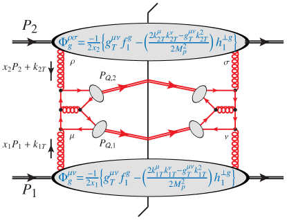
TMD factorization extends collinear factorization by taking into account the intrinsic TM of the partons, usually denoted by $\mbox{\boldmath$k$}_{{\scriptscriptstyle T}}$. As in collinear factorization, the hard-scattering amplitude, which can be perturbatively computed, is multiplied by parton correlators that can be parametrized in terms of parton distribution functions, but in this case $\mbox{\boldmath$k$}_{{\scriptscriptstyle T}}$ dependent. The parametrization of parton correlators is an extension from that used in collinear factorization, not only because of the $\mbox{\boldmath$k$}_{{\scriptscriptstyle T}}$ dependence of the distribution functions, but also because there are more distributions. The gluon correlator inside an unpolarized proton with momentum $P$ and mass $M_{p}$, denoted by $\Phi_{g}^{\mu\nu}(x,\mbox{\boldmath$k$}_{{\scriptscriptstyle T}})$ Mulders:2000sh ; Meissner:2007rx ; Boer:2016xqr , can be parametrized in terms of two independent TMDs. The first one is the distribution of unpolarized gluons $f_{1}^{\,g}(x,\mbox{\boldmath$k$}_{{\scriptscriptstyle T}}^{2})$, the second one is the distribution of linearly polarized gluons $h_{1}^{\perp\,g}(x,\mbox{\boldmath$k$}_{{\scriptscriptstyle T}}^{2})$. Here the gluon 4-momentum is written using a Sudakov decomposition: $k=xP+k_{{\scriptscriptstyle T}}+k^{-}n$ (where $n$ is any light-like vector ($n^{2}=0$) such that $n\cdot P\neq 0$), where $\mbox{\boldmath$k$}_{\scriptscriptstyle T}^{2}=-k_{\scriptscriptstyle T}^{2}$ and the transverse metric is $g^{\mu\nu}_{{\scriptscriptstyle T}}=g^{\mu\nu}-(P^{\mu}n^{\nu}+P^{\nu}n^{\mu})/P{\cdot}n$. For TMD factorization to hold, the hard scale of the process should be much larger than the pair TM, $q_{T}$.

The process we are interested in is the fusion of two gluons coming from two colliding unpolarized protons, leading to the production of a pair of vector $S$-wave quarkonia: $g(k_{1}){+}g(k_{2})\to{\cal Q}(P_{{\cal Q},1}){+}{\cal Q}(P_{{\cal Q},2})\,$. The cross-section for this reaction involves the contraction of two gluon correlators Lansberg:2017dzg , $\Phi_{g}^{\mu\nu}(x_{1},\mbox{\boldmath$k$}_{1{\scriptscriptstyle T}})$ and $\Phi_{g}^{\rho\sigma}(x_{2},\mbox{\boldmath$k$}_{2{\scriptscriptstyle T}})$, with the squared amplitude $\mathcal{M}^{\mu\rho}(\mathcal{M}^{\nu\sigma})^{*}$ of the partonic scattering, integrated over the gluon momenta. The expression of the tree-level partonic amplitude $\mathcal{M}$ is available in Qiao:2009kg , although the earliest computations date back to 1983 Kartvelishvili:1984ur ; Humpert:1983yj . The hadronization process, i.e. the transition from a heavy-quark pair to a quarkonium bound state, is described in our study using the color singlet model (CSM) Chang:1979nn ; Baier:1981uk ; Baier:1983va or in this case equivalently non-relativistic QCD (NRQCD) Bodwin:1994jh at LO in the velocity $v$ of the heavy quarks in the bound-state rest frame. Fig. 1 represents the complete reaction with a typical Feynman diagram depicting the partonic subprocess.

2.2 Other contributions to quarkonium-pair production

The leading contribution to the hadronization of a $Q\overline{Q}$ pair into a bound state in NRQCD is the Color-Singlet (CS) transition, for which the perturbatively-produced heavy-quark pair has the same quantum numbers as the quarkonium and directly binds without any extra soft interaction. Corrections to this leading contribution involving higher Color-Octet (CO) Fock states are suppressed by powers of $v$, which is meant to be much smaller than unity for heavy quarkonia.

The CS over CO dominance normally follows from this power suppression in $v$ encoded in the so-called NRQCD long distance matrix elements (LDMEs). More precisely one expects a relative suppression on the order of $v^{4}$ Bodwin:1994jh ; Cho:1995ce ; Cho:1995vh (see Lansberg:2019adr ; Andronic:2015wma ; Brambilla:2010cs ; Lansberg:2006dh for reviews) per quarkonium. For di-$J/\psi$ production with $v^{2}_{c}\simeq 0.25$ and for which both the CO and the CS yields are produced at $\alpha_{s}^{4}$, the CO/CS yield ratio, which thus scales as $v_{c}^{8}$, likely lies below the percent level. Explicit computations Ko:2010xy ; Li:2013csa ; Lansberg:2014swa ; He:2015qya ; Lansberg:2019fgm indeed show corrections from the CO states below the percent level except in some corners of the phase space (e.g. large rapidity separation $\Delta y$) where some CO contributions can be kinematically enhanced, but these can safely be avoided with appropriate kinematical cuts. More details can be found in Lansberg:2019fgm .

It is important for the applicability of TMD factorization that the CS contributions dominate. Soft gluon interactions between the hadrons and a colored initial or final state of the hard scattering can be encapsulated within the definition of the TMD through the use of Wilson lines. However, if both initial and final states are subject to soft gluon interactions, the resulting color entanglement may break TMD factorization Collins:2007nk ; Collins:2007jp ; Rogers:2010dm . The dominance of the CS contributions should therefore be ensured.

It is also important to take into account $\alpha_{s}$ corrections. In the TMD region, $\boldsymbol{P}_{{\cal Q}{\cal Q}{\scriptscriptstyle T}}\ll M_{{\cal Q}{\cal Q}}$, these introduce a renormalization scale ($\mu$) dependence in the TMD correlators and a rapidity scale $\zeta$ dependence Collins:2011zzd ; GarciaEchevarria:2011rb ; Echevarria:2012js . At larger $\boldsymbol{P}_{{\cal Q}{\cal Q}{\scriptscriptstyle T}}$ one has to match onto the collinear factorization expression (see e.g. Echevarria:2018qyi ), which is calculated by taking real-gluon emissions into account Lansberg:2013qka ; Lansberg:2014swa ; Sun:2014gca ; Likhoded:2016zmk . At finite $\boldsymbol{P}_{{\cal Q}{\cal Q}{\scriptscriptstyle T}}$, such single real-gluon emissions occur at $\alpha_{s}^{5}$ and the quarkonium pair effectively recoils against this hard gluon, increasing the pair TM. In this paper we will restrict to $\boldsymbol{P}_{{\cal Q}{\cal Q}{\scriptscriptstyle T}}<M_{{\cal Q}{\cal Q}}/2$ in order to stay away from the matching region.

Thus far, we have focused our discussion on the single parton scattering (SPS) case. However, since we look at a two-particle final state, we should also consider the case where the quarkonia are created in two separate hard scatterings, i.e. double parton scattering (DPS). At LHC energies, the gluon densities are typically high and the likelihood for two hard gluon fusions to take place during the same proton-proton scattering cannot be neglected.

In the case of di-$J/\psi$, it has been already anticipated in 2011 Kom:2011bd that DPS contributions may be dominant at large rapidity difference $\Delta y$ (thus large invariant masses with same individual TM). This was corroborated Lansberg:2014swa by the CMS data Khachatryan:2014iia with an excess above the SPS predictions at large $\Delta y$. ATLAS further Aaboud:2016fzt confirmed the DPS relevance in di-$J/\psi$ production with a dedicated DPS study. One expects Lansberg:2014swa ; Aaboud:2016fzt that DPS contributions lie below 10% for $\Delta y\sim 0$ in the CMS and ATLAS samples (characterized by a $P_{{\cal Q}T}$ cut away from the threshold $M_{\psi\psi}\simeq 2M_{\psi}$) and that they only matter at large $\Delta y$. However, in the LHCb acceptance (where $M_{\psi\psi}\simeq 2M_{\psi}$), DPS contributions cannot a priori be neglected, but can be subtracted Aaij:2016bqq if one assumes that, for the DPS sample, the kinematics of both $J/\psi$’s is uncorrelated. This yield a precise (yet, unnormalized) prediction of the kinematical distributions.

Another source of quarkonium pairs is the feed-down from excited states. For $J/\psi$-pair production, the main feed-down sources are the $\chi_{c}$ and $\psi^{\prime}$. The feed-down from $\chi_{c}$ is expected to be small, as $gg\rightarrow J/\psi+\chi_{c}$ and $gg\rightarrow\psi^{\prime}+\chi_{c}$ are suppressed Lansberg:2014swa at LO by $C$-parity and the vanishing of the $\chi_{c}$ wave function at the origin, and $gg\rightarrow\chi_{c}+\chi_{c}$ is suppressed by the squared $\chi_{c}\rightarrow J/\psi$ branching ratio. The production of a $\psi^{\prime}$ with a $J/\psi$ likely contributes Lansberg:2019adr 50% of the $J/\psi$-pair samples, owing to the large branching ratio for $\psi^{\prime}\to J/\psi$ (${\cal O}(60)\%$) and symmetry factors. Yet, $\psi^{\prime}+J/\psi$ pairs are produced exactly like $J/\psi+J/\psi$ pairs and thus generate the same TMD observables .

In the case of $\Upsilon$-pair production, the main feed-down is from $\Upsilon(2,\!3S)$. According to Berezhnoy:2012tu , less than 30% of the produced pairs would originate from feed-down at $\sqrt{s}$ = 8 TeV. As in the $J/\psi$ case, $C$-parity suppresses the $\Upsilon+\chi_{b}$ reaction at leading order, and $\chi_{b}+\chi_{b}$ is suppressed by the squared branching ratio. Regarding the CO contributions, the relative velocity of the quarks inside the $\Upsilon$ is smaller than for the $J/\psi$, meaning the NRQCD expansion used to describe the hadronization has a better convergence. Therefore it is highly unlikely that the CO channels overcome the CS ones in the reachable phase space. The fraction of DPS events is also expected to be less than 5% at low $\boldsymbol{P}_{{\cal Q}{\cal Q}{\scriptscriptstyle T}}$ and central rapidity Lansberg:2019adr , making it an overall cleaner process.

2.3 The TMD differential cross-section

The general structure of the TMD-based differential cross-section describing quarkonium-pair production from gluon fusion reads Lansberg:2017dzg :

$$\frac{\mathrm{d}\sigma}{\mathrm{d}M_{{\cal Q}{\cal Q}}\mathrm{d}Y_{{\cal Q}{\cal Q}}\mathrm{d}^{2}\boldsymbol{P}_{{\cal Q}{\cal Q}{\scriptscriptstyle T}}\mathrm{d}\Omega}=\frac{\sqrt{M_{{\cal Q}{\cal Q}}^{2}-4M_{\mathcal{Q}}^{2}}}{(2\pi)^{2}8s\,M_{{\cal Q}{\cal Q}}^{2}}$$ (1)

$$\Bigg{\{} F_{1}(M_{{\cal Q}{\cal Q}},\theta_{{\rm CS}})\ \mathcal{C}\Big{[}f_{1}^{g}f_{1}^{g}\Big{]}(x_{1,2},\boldsymbol{P}_{{\cal Q}{\cal Q}{\scriptscriptstyle T}})$$

$$+ F_{2}(M_{{\cal Q}{\cal Q}},\theta_{{\rm CS}})\ \mathcal{C}\Big{[}w_{2}h_{1}^{\perp g}h_{1}^{\perp g}\Big{]}(x_{1,2},\boldsymbol{P}_{{\cal Q}{\cal Q}{\scriptscriptstyle T}})$$

$$+ \Bigg{(}F_{3}(M_{{\cal Q}{\cal Q}},\theta_{{\rm CS}})\ \mathcal{C}\Big{[}w_{3}f_{1}^{g}h_{1}^{\perp g}\Big{]}(x_{1,2},\boldsymbol{P}_{{\cal Q}{\cal Q}{\scriptscriptstyle T}})+$$

$$F^{\prime}_{3}(M_{{\cal Q}{\cal Q}},\theta_{{\rm CS}})\ \mathcal{C}\Big{[}w^{\prime}_{3}h_{1}^{\perp g}f_{1}^{g}\Big{]}(x_{1,2},\boldsymbol{P}_{{\cal Q}{\cal Q}{\scriptscriptstyle T}})\Bigg{)}\cos 2\phi_{{\rm CS}}\$$

$$+ F_{4}(M_{{\cal Q}{\cal Q}},\theta_{{\rm CS}})\ \mathcal{C}\!\left[w_{4}h_{1}^{\perp g}h_{1}^{\perp g}\right](x_{1,2},\boldsymbol{P}_{{\cal Q}{\cal Q}{\scriptscriptstyle T}})\cos 4\phi_{{\rm CS}}\!\Bigg{\}}\,,$$

with $\mathrm{d}\Omega=\mathrm{d}\!\cos\theta_{{\rm CS}}\mathrm{d}\phi_{{\rm CS}}$, $\{\theta_{{\rm CS}},\phi_{{\rm CS}}\}$ being the Collins-Soper (CS) angles Collins:1977iv , and $Y_{{\cal Q}{\cal Q}}$ is the rapidity of the pair. $x_{1,2}=M_{{\cal Q}{\cal Q}}\,e^{\pm Y_{{\cal Q}{\cal Q}}}/\sqrt{s}$, with $s=(P_{1}+P_{2})^{2}$. Here $\boldsymbol{P}_{{\cal Q}{\cal Q}{\scriptscriptstyle T}}$ ($\equiv q_{T}$) and $Y_{{\cal Q}{\cal Q}}$ are defined in the hadron c.m.s. The quarkonia move along (in the opposite direction) $\vec{e}=(\sin\theta_{{\rm CS}}\cos\phi_{{\rm CS}},\sin\theta_{{\rm CS}}\sin\phi_{{\rm CS}},\cos\theta_{{\rm CS}})$ in the CS frame. The kinematical pre-factor is specific to the mass of the quarkonia and the considered differential cross-sections, while the hard-scattering coefficients $F_{i}$ only depend on $\theta_{{\rm CS}}$ and the invariant mass of the system, here $M_{{\cal Q}{\cal Q}}$. Their expression for quarkonium-pair production can be found at tree level in Lansberg:2017dzg . When $P_{{\cal Q}T}\gg M_{\cal Q}$, small values of $\cos\theta_{{\rm CS}}$ correspond to small values of $\Delta y$ in the hadron c.m.s.

The TMD convolutions appearing in Eq. (1) are defined as follows:

$$\mathcal{C}[w\,f\,g](x_{1,2},\boldsymbol{P}_{{\cal Q}{\cal Q}{\scriptscriptstyle T}})\equiv$$

$$\int\!\!\mathrm{d}^{2}\mbox{\boldmath$k$}_{1{\scriptscriptstyle T}}\!\!\int\!\!\mathrm{d}^{2}\mbox{\boldmath$k$}_{2{\scriptscriptstyle T}}\,\delta^{2}(\mbox{\boldmath$k$}_{1{\scriptscriptstyle T}}+\mbox{\boldmath$k$}_{2{\scriptscriptstyle T}}-{\boldsymbol{P}_{{\cal Q}{\cal Q}{\scriptscriptstyle T}}})\times$$

$$w(\mbox{\boldmath$k$}_{1{\scriptscriptstyle T}},\mbox{\boldmath$k$}_{2{\scriptscriptstyle T}})\,f(x_{1},\mbox{\boldmath$k$}_{1{\scriptscriptstyle T}}^{2})\,g(x_{2},\mbox{\boldmath$k$}_{2{\scriptscriptstyle T}}^{2})\,,$$ (2)

where $w(\mbox{\boldmath$k$}_{1{\scriptscriptstyle T}},\mbox{\boldmath$k$}_{2{\scriptscriptstyle T}})$ denotes a TMD weight. The weights in Eq. (1) are common to all gluon-fusion processes originating from unpolarized proton collisions. They can be found in Lansberg:2017tlc . Our aim in the present study is to study the impact of QCD evolution effects in the above TMD convolutions. Having at our disposal the computation of the hard-scattering coefficients, the measurements of differential yields in principle allow one to extract these TMD convolutions evolved up to the natural scale of the process, on the order of $M_{{\cal Q}{\cal Q}}$ here.

In practice, one looks at specific observables sensitive to these convolutions. First we note that when the cross-section is integrated over the azimuthal angle $\phi_{{\rm CS}}$ , the terms with a $\cos(2,\!4\phi_{{\rm CS}})$-dependence drop out from Eq. (1) such that

$$\frac{1}{2\pi} \int\!\!d\phi_{{\rm CS}}\frac{d\sigma}{dM_{{\cal Q}{\cal Q}}dY_{{\cal Q}{\cal Q}}d^{2}\boldsymbol{P}_{{\cal Q}{\cal Q}{\scriptscriptstyle T}}d\Omega}=$$

$$F_{1}\,\mathcal{C}\Big{[}f_{1}^{\,g}f_{1}^{\,g}\Big{]}+F_{2}\,\mathcal{C}\Big{[}w_{2}h_{1}^{\perp\,g}h_{1}^{\perp\,g}\Big{]}\,,$$ (3)

giving direct access to $\mathcal{C}\Big{[}f_{1}^{\,g}f_{1}^{\,g}\Big{]}$ and $\mathcal{C}\Big{[}w_{2}h_{1}^{\perp\,g}h_{1}^{\perp\,g}\Big{]}$.

Furthermore, one can define, at fixed $\{Y,\boldsymbol{P}_{{\cal Q}{\cal Q}{\scriptscriptstyle T}},\theta_{{\rm CS}},M_{{\cal Q}{\cal Q}}\}$, $\cos(n\phi_{{\rm CS}})$-weighted differential cross-sections, integrated over $\phi_{{\rm CS}}$ and normalized by their azimuthally-independent component:

$$\langle\cos(n\phi_{{\rm CS}})\rangle=$$

$$\frac{\displaystyle\int\!\!d\phi_{{\rm CS}}\cos(n\phi_{{\rm CS}})\,\frac{\displaystyle\mathrm{d}\sigma}{dM_{{\cal Q}{\cal Q}}dY_{{\cal Q}{\cal Q}}d^{2}\boldsymbol{P}_{{\cal Q}{\cal Q}{\scriptscriptstyle T}}d\Omega}}{\displaystyle\!\!\int\!\!d\phi_{{\rm CS}}\frac{d\sigma}{dM_{{\cal Q}{\cal Q}}dY_{{\cal Q}{\cal Q}}d^{2}\boldsymbol{P}_{{\cal Q}{\cal Q}{\scriptscriptstyle T}}d\Omega}}\,.$$ (4)

Such a variable, computed for $n$ = 2 or 4 in our case, corresponds to (half of) the relative size of the $\cos(2,\!4\phi_{{\rm CS}})$-modulations present in the TMD cross-section in comparison to its $\phi_{{\rm CS}}$-independent component:

$$\langle\cos 2\phi_{{\rm CS}}\rangle = \frac{1}{2}\;\frac{F_{3}\mathcal{C}\Big{[}w_{3}f_{1}^{\,g}h_{1}^{\perp\,g}\Big{]}+F^{\prime}_{3}\mathcal{C}\Big{[}w^{\prime}_{3}h_{1}^{\perp\,g}f_{1}^{\,g}\Big{]}}{F_{1}\,\mathcal{C}\Big{[}f_{1}^{\,g}f_{1}^{\,g}\Big{]}+F_{2}\,\mathcal{C}\Big{[}w_{2}h_{1}^{\perp\,g}h_{1}^{\perp\,g}\Big{]}}\,,$$

$$\langle\cos 4\phi_{{\rm CS}}\rangle = \frac{1}{2}\;\frac{F_{4}\mathcal{C}\!\left[w_{4}h_{1}^{\perp\,g}h_{1}^{\perp\,g}\right]}{F_{1}\,\mathcal{C}\Big{[}f_{1}^{\,g}f_{1}^{\,g}\Big{]}+F_{2}\,\mathcal{C}\Big{[}w_{2}h_{1}^{\perp\,g}h_{1}^{\perp\,g}\Big{]}}\,.$$ (5)

When $\langle\cos n\phi_{{\rm CS}}\rangle$ is computed within a range of $M_{{\cal Q}{\cal Q}}$, $Y_{{\cal Q}{\cal Q}}$, $\boldsymbol{P}_{{\cal Q}{\cal Q}{\scriptscriptstyle T}}$ or $\cos(\theta_{{\rm CS}})$, we define it as the ratio of corresponding integrals. Of course, the range in $\boldsymbol{P}_{{\cal Q}{\cal Q}{\scriptscriptstyle T}}$ should be such that one remains in the TMD region, i.e. $\boldsymbol{P}_{{\cal Q}{\cal Q}{\scriptscriptstyle T}}\ll M_{{\cal Q}{\cal Q}}$.

For positive Gaussian $h_{1}^{\perp\,g}$ the $\langle\cos(2\phi_{CS})\rangle$ asymmetry will be positive (note that in Lansberg:2017dzg the $\langle\cos(2\phi_{CS})\rangle$ plots miss an overall minus sign).

3 TMD evolution formalism

TMD evolution has been considered in an increasing number of TMD observables. It is usually implemented by Fourier transforming to $b_{T}$-space, with $b_{T}$ being the conjugate variable to $\boldsymbol{P}_{{\cal Q}{\cal Q}{\scriptscriptstyle T}}$. When evolution effects are considered, the TMDs acquire a dependence on two scales: a renormalization scale $\mu$ and a rapidity scale $\zeta$ (whose evolution is governed by the Collins-Soper equation). Below we present in a simple way the results needed to perform the TMD evolution. For more details, we refer to e.g. Collins:2011ca ; Echevarria:2012pw ; Echevarria:2014rua ; Echevarria:2015uaa .

When TMD evolution is incorporated to the gluon TMDs in the tree-level result in Eq. (1), the convolutions take the form

$$\mathcal{C} [w\,f\,g](x_{1,2},\boldsymbol{P}_{{\cal Q}{\cal Q}{\scriptscriptstyle T}};\mu)\equiv$$

$$\int\!\!\mathrm{d}^{2}\mbox{\boldmath$k$}_{1{\scriptscriptstyle T}}\!\!\int\!\!\mathrm{d}^{2}\mbox{\boldmath$k$}_{2{\scriptscriptstyle T}}\,\delta^{2}(\mbox{\boldmath$k$}_{1{\scriptscriptstyle T}}+\mbox{\boldmath$k$}_{2{\scriptscriptstyle T}}-{\boldsymbol{P}_{{\cal Q}{\cal Q}{\scriptscriptstyle T}}})\times$$

$$w(\mbox{\boldmath$k$}_{1{\scriptscriptstyle T}},\mbox{\boldmath$k$}_{2{\scriptscriptstyle T}})\,f(x_{1},\mbox{\boldmath$k$}_{1{\scriptscriptstyle T}}^{2};\zeta_{1},\mu)\,g(x_{2},\mbox{\boldmath$k$}_{2{\scriptscriptstyle T}}^{2};\zeta_{2},\mu)\,,$$ (6)

where the two rapidity scales should fulfill the constraint $\zeta_{1}\zeta_{2}=M_{{\cal Q}{\cal Q}}^{4}$. While the renormalization scale $\mu$ in the hard-scattering coefficients $F_{i}$ should be set here to $\mu\sim M_{{\cal Q}{\cal Q}}$ in order to avoid large logarithms, the TMDs should be evaluated at their natural scale $\mu\sim\sqrt{\zeta}\sim\mu_{b}=b_{0}/b_{T}$ (with $b_{0}=2e^{-\gamma_{E}}$), in order to minimize both logarithms of $\mu b_{T}$ and $\zeta b_{T}^{2}$, and then evolved up to $\mu\sim\sqrt{\zeta}\sim M_{{\cal Q}{\cal Q}}$. The solution of the evolution equations results in the introduction of the following Sudakov factor $S_{A}$:

$$\tilde{f}_{1}^{\,g}(x_{1},b_{T}^{2};\zeta,\mu) = e^{-\frac{1}{2}S_{A}(b_{T};\zeta,\mu)}\tilde{f}_{1}^{\,g}(x,b_{T}^{2};\mu_{b}^{2},\mu_{b})\,,$$

$$\tilde{h}_{1}^{\perp\,g}(x_{1},b_{T}^{2};\zeta,\mu) = e^{-\frac{1}{2}S_{A}(b_{T};\zeta,\mu)}\tilde{h}_{1}^{\perp\,g}(x,b_{T}^{2};\mu_{b}^{2},\mu_{b})$$ (7)

where the Fourier-transformed TMDs are

$$\tilde{f}_{1}^{\,g}(x,\mbox{\boldmath$b$}_{T}^{2};\zeta,\mu) = \int\!d^{2}\mbox{\boldmath$k$}_{T}\,e^{-i\mbox{\boldmath${\scriptstyle b}$}_{T}\cdot\,\mbox{\boldmath${\scriptstyle k}$}_{T}}f_{1}^{\,g}(x,\mbox{\boldmath$k$}_{T}^{2};\zeta,\mu)\,,$$

$$\tilde{h}_{1}^{\perp\,g}(x,\mbox{\boldmath$b$}_{T}^{2};\zeta,\mu) = \int\!d^{2}\mbox{\boldmath$k$}_{T}\,\frac{(\mbox{\boldmath$b$}_{T}\cdot\,\mbox{\boldmath$k$}_{T})^{2}-\frac{1}{2}\mbox{\boldmath$b$}_{T}^{2}\mbox{\boldmath$k$}_{T}^{2}}{\mbox{\boldmath$b$}_{T}^{2}M_{p}^{2}}$$ (8)

$$\times e^{-i\mbox{\boldmath${\scriptstyle b}$}_{T}\cdot\,\mbox{\boldmath${\scriptstyle k}$}_{T}}h_{1}^{\perp\,g}(x,\mbox{\boldmath$k$}_{T}^{2};\zeta,\mu)\,,$$

and the perturbative Sudakov factor (applicable for sufficiently small $b_{T}$) is given by

$$S_{A}(b_{T};\zeta,\mu) =2D(\mu_{b}^{2})\,\ln\frac{\zeta}{\mu_{b}^{2}}+$$ (9)

$$2\int_{\mu_{b}}^{\mu}\!\!\frac{d\bar{\mu}}{\bar{\mu}}\Bigg{[}\Gamma(\alpha_{s}(\bar{\mu}^{2}))\ln\frac{\zeta}{\bar{\mu}^{2}}+\gamma(\alpha_{s}(\bar{\mu}^{2}))\Bigg{]}\,.$$

We consider here the resummation at next-to-leading-logarithmic accuracy, for which the Collins-Soper kernel $D$ and the non-cusp anomalous dimension $\gamma$ need to be taken at leading-order, while the cusp anomalous dimension $\Gamma$ at next-to-leading-order. The perturbative Sudakov factor then takes the form

$$S_{A}(b_{T};\zeta,\mu)=2\frac{C_{A}}{\pi}\int_{\mu_{b}}^{\mu}\!\!\frac{d\bar{\mu}}{\bar{\mu}}\ln\left(\frac{\zeta}{\bar{\mu}^{2}}\right)$$ (10)

$$\times\Bigg{[}\alpha_{s}(\bar{\mu}^{2})+\bigg{(}\big{(}\frac{67}{9}-\frac{\pi^{2}}{3}\big{)}-\frac{20T_{f}n_{f}}{9}\bigg{)}\frac{\alpha_{s}^{2}(\bar{\mu}^{2})}{4\pi}\Bigg{]}$$

$$\quad+2\frac{C_{A}}{\pi}\int_{\mu_{b}}^{\mu}\!\!\frac{d\bar{\mu}}{\bar{\mu}}\alpha_{s}(\bar{\mu}^{2})\left[-\frac{11-2n_{f}/C_{A}}{6}\right]\,,$$ (11)

with $C_{A}=3$, $T_{f}=1/2$ and $n_{f}$ the number of flavors (we will use $n_{f}=4$ for di-$J/\psi$ and $n_{f}=5$ for di-$\Upsilon$ production). The running of $\alpha_{s}$ is implemented at one loop. We note that the Sudakov factor $S_{A}$ is spin independent, and thus the same for all (un)polarized TMDs Echevarria:2014rua ; Echevarria:2015uaa .

The perturbative component of the TMDs for small $b_{T}$ can be computed at a given order in $\alpha_{s}$. At leading order, $\tilde{f}_{1}^{\,g}$ is given by the integrated PDF:

$$\tilde{f}_{1}^{\,g}(x,b_{T}^{2};\zeta,\mu)=f_{g/P}(x;\mu)+\mathcal{O}(\alpha_{s})+\mathcal{O}(b_{T}\Lambda_{\rm QCD})\,.$$ (12)

As said above, $h_{1}^{\perp\,g}$ describes the correlation between the gluon polarization and its TM ($k_{T}$) inside the unpolarized proton. It requires a helicity flip and therefore an additional gluon exchange. Consequently, its perturbative expansion starts at $\mathcal{O}(\alpha_{s})$ Sun:2011iw :

$$\tilde{h}_{1}^{\,\perp g}(x,b_{T}^{2};\zeta,\mu)=-\!\left(\frac{\alpha_{s}(\mu)C_{A}}{\pi}\!\!\int_{x}^{1}\!\!\frac{d\hat{x}}{\hat{x}}\!\!\left(\frac{\hat{x}}{x}-1\right)\!\!f_{g/P}(\hat{x};\mu)\right.$$

$$+\frac{\alpha_{s}(\mu)C_{F}}{\pi}\sum_{i=q,\bar{q}}\int_{x}^{1}\!\!\left.\frac{d\hat{x}}{\hat{x}}\left(\frac{\hat{x}}{x}-1\right)f_{i/P}(\hat{x};\mu)\right)$$

$$+\mathcal{O}(\alpha_{s}^{2})+\mathcal{O}(b_{T}\Lambda_{\rm QCD})\,,$$ (13)

The above equations in principle allow one to derive a perturbative expression of these TMDs. However, they are strictly applicable only in a restricted $b_{T}$ range, whereas we need an expression for them from small to large $b_{T}$ in order to perform the corresponding Fourier transform.

For large $b_{T}$, one indeed leaves the domain of perturbation theory. On the contrary, when $b_{T}$ gets too small, $\mu_{b}$ becomes larger than $M_{{\cal Q}{\cal Q}}$ and the evolution should stop. The above perturbative expression for the Sudakov factor should thus not be used as it is.

One of the common solutions to continue to use the above expressions consists in replacing $b_{T}$ by a function of $b_{T}$ which freezes in both these limits such that one is not sensitive to the physics there. For our numerical studies we use the following $b_{T}$ prescription Collins:2016hqq :

$$b_{T}^{*}\big{(}b_{c}(b_{T})\big{)} =\frac{b_{c}(b_{T})}{\sqrt{1+\Big{(}\frac{b_{c}(b_{T})}{b_{T_{\max}}}\Big{)}^{2}}}$$ (14)

where

$$b_{c}(b_{T})=\sqrt{b_{T}^{2}+\Big{(}\frac{b_{0}}{M_{{\cal Q}{\cal Q}}}\Big{)}^{2}}\,,$$ (15)

such that $\mu_{b}=\frac{b_{0}}{b_{T}^{*}(b_{c})}$ always lies between $b_{0}/b_{T_{\max}}$ (reached when $b_{T}\rightarrow\infty$) and $M_{{\cal Q}{\cal Q}}$ (reached when $b_{T}\rightarrow 0$). This prescription is of course not unique, as it entails e.g. some particular assumptions on the transition from the hard to the soft regime. The ambiguity in the choice of this prescription can however be absorbed in the nonperturbative modelling of the TMDs, anyhow needed in the large $b_{T}$ region, which we discuss next.

Schematically each TMD convolution can be written in $b_{T}$-space as

$$\mathcal{C}[w\,f\,g]=\int_{0}^{\infty}\!\!\frac{db_{T}}{2\pi}\,b_{T}^{n}J_{m}(b_{T}q_{T})\,\tilde{W}(b_{T},Q)\,,$$ (16)

for some integers $n$ and $m$. Here $\tilde{W}$ is a simple product of Fourier-transformed TMDs. The nonperturbative Sudakov factor $S_{{\rm NP}}$ is now defined through $\tilde{W}(b_{T},Q)=\tilde{W}(b_{T}^{*},Q)\,e^{-S_{{\rm NP}}(b_{T},Q)}$, where by construction $\tilde{W}(b_{T}^{*},Q)$ is perturbatively calculable for all $b_{T}$ values. The value of $b_{T\max}$ in Eq. (14) (roughly) sets the separation between the perturbative and nonperturbative domains. Its optimal value depends on many factors, such as the functional form chosen for $b_{T}^{*}$ and the parametrization of the nonperturbative Sudakov factor $S_{{\rm NP}}$. For our numerical studies we take $b_{T\max}=1.5$ GeV^-1, inspired by previous fits from Drell-Yan and $W,Z$ production Landry:2002ix ; Konychev:2005iy ; Aybat:2011zv ; Collins:2014jpa ; DAlesio:2014mrz .

The functional form of $S_{{\rm NP}}$ has been subject of debate, but is usually chosen to be proportional to $b_{T}^{2}$ for all $b_{T}$. By definition $e^{-S_{{\rm NP}}(b_{T},Q)}$ has to be equal to 1 for $b_{T}=0$ and for large $b_{T}$ it has to vanish, at the very least to ensure convergence of the results. It is usually assumed to be a monotonically decreasing function of $b_{T}$ and its change from 1 to 0 is assumed to happen within the confinement distance. Lacking experimental constraints, here we will assume a simple Gaussian form (of varying widths). In order to assess the importance of the nonperturbative Sudakov factor for the size of the asymmetries and to perform a first error estimate, we consider several functions. For this purpose, we take a simple formula for the nonperturbative Sudakov factor that encapsulates the expected $M_{{\cal Q}{\cal Q}}$-dependence Collins:1981va and the assumed $b_{T}$-Gaussian behavior:

$$S_{{\rm NP}}\big{(}b_{c}(b_{T})\big{)}=A\ln\Big{(}\frac{M_{{\cal Q}{\cal Q}}}{Q_{\rm NP}}\Big{)}\,b_{c}^{2}(b_{T})\,,\qquad Q_{\rm NP}=1~{}{\rm GeV}\,.$$ (17)

From this nonperturbative Sudakov factors a value $b_{T\lim}$ is defined at which $e^{-S_{{\rm NP}}}$ becomes negligible, to be specific, where it becomes $\sim$ 10^-3. From this we furthermore define a corresponding characteristic radius $r=\tfrac{1}{2}b_{T\lim}$ (considering $b_{T\lim}$ the diameter, since it is conjugate to $\boldsymbol{P}_{{\cal Q}{\cal Q}{\scriptscriptstyle T}}=\mbox{\boldmath$k$}_{1T}+\mbox{\boldmath$k$}_{2T}$), which delimits the range over which the interactions occur from the center of the proton. To estimate the uncertainty associated with the largely unknown nonperturbative Sudakov factor, we will consider three cases: $b_{T\lim}$ $=$ 2, 4 and 8 GeV^-1. This spans roughly from $b_{T\max}=1.5$ GeV^-1 to the charge radius of the proton. The corresponding values of the parameter $A$ and $r$ for $M_{{\cal Q}{\cal Q}}=12$ GeV are given in Table 1.

$A$ (GeV2)	$b_{T\lim}$ (GeV-1)	$r$ (fm $\sim 1/(0.2~{}{\rm GeV}$)
0.64	2	0.2
0.16	4	0.4
0.04	8	0.8

Table 1: Values of the parameter $A$ used in Eq. (17) for $e^{-S_{{\rm NP}}}$, along with the corresponding $b_{T\lim}$ and $r$ at $M_{{\cal Q}{\cal Q}}=12$ GeV

The value $M_{{\cal Q}{\cal Q}}=12$ GeV is considered because the ratio $F_{3}/F_{1}$ peaks there (for $J/\psi$ pair production), but we will also consider larger values later on. When $M_{{\cal Q}{\cal Q}}$ increases, the interaction radius $r$ decreases. Fig. 2 depicts $e^{-S_{{\rm NP}}}$ as a function of $b_{T}$ for the three values of $A$ previously mentioned and for $M_{{\cal Q}{\cal Q}}$ ranging from 12 to 30 GeV.

Figure 2: $e^{-S_{{\rm NP}}}$ from Eq. (17) vs $b_{T}$ for $A$ $=$ 0.04 (purple), 0.16 (orange) and 0.64 (magenta) GeV², for values of $M_{{\cal Q}{\cal Q}}$ ranging from 12 to 30 GeV. The boundaries around the bands depict the exponential at $M_{{\cal Q}{\cal Q}}$=12 GeV (solid line) and at $M_{{\cal Q}{\cal Q}}$=30 GeV (dotted line).

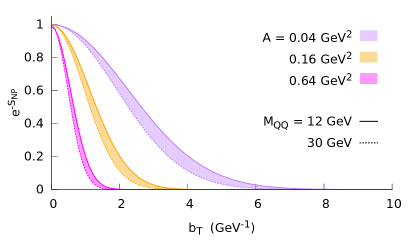
We point out that the nonperturbative Sudakov factor as fitted by Aybat and Rogers Aybat:2011zv to low-energy SIDIS as well as high-energy Drell-Yan and $Z^{0}$ production data, rescaled by a color factor $C_{A}/C_{F}$ to account for the different color representation between quarks and gluons, is very close to the case $b_{T\lim}$ $=$ 2 GeV^-1. It is also very close to the Fourier transform of the Gaussian model for $f_{1}^{g}(x,k_{T}^{2})$ with $\langle k_{T}^{\,2}\rangle=3.3\pm 0.8$ GeV² as extracted in Lansberg:2017dzg from a LO fit to $J/\psi$-pair-production data from LHCb Aaij:2016bqq from which the DPS contributions was however approximately subtracted.

We end this section by providing the expressions for the TMD convolutions in $b_{T}$-space, which we actually use in the numerical predictions in the next section:

$$\mathcal{C}\Big{[}f_{1}^{\,g}f_{1}^{\,g}\Big{]}\!=\!\int_{0}^{\infty}\!\!\frac{db_{T}}{2\pi}\,b_{T}J_{0}(b_{T}q_{T})\,e^{-S_{A}(b_{T}^{*};M_{{\cal Q}{\cal Q}}^{2},M_{{\cal Q}{\cal Q}})}\,$$

$$\times e^{-S_{{\rm NP}}(b_{c})}\tilde{f}_{1}^{\,g}(x_{1},b_{T}^{*\,2};\mu_{b}^{2},\mu_{b})\,\tilde{f}_{1}^{\,g}(x_{2},b_{T}^{*\,2};\mu_{b}^{2},\mu_{b})\,,$$

$$\mathcal{C}\Big{[}w_{2}\,h_{1}^{\perp\,g}h_{1}^{\perp\,g}\Big{]}\!=\!\int_{0}^{\infty}\!\!\frac{db_{T}}{2\pi}\,b_{T}J_{0}(b_{T}q_{T})\,e^{-S_{A}(b_{T}^{*};M_{{\cal Q}{\cal Q}}^{2},M_{{\cal Q}{\cal Q}})}\,$$

$$\times e^{-S_{{\rm NP}}(b_{c})}\tilde{h}_{1}^{\perp\,g}(x_{1},b_{T}^{*\,2};\mu_{b}^{2},\mu_{b})\,\tilde{h}_{1}^{\perp\,g}(x_{2},b_{T}^{*\,2};\mu_{b}^{2},\mu_{b})\,,$$

$$\mathcal{C}\Big{[}w_{3}\,f_{1}^{\,g}h_{1}^{\perp\,g}\Big{]}\!=\!\int_{0}^{\infty}\!\!\frac{db_{T}}{2\pi}\,b_{T}J_{2}(b_{T}q_{T})\,e^{-S_{A}(b_{T}^{*};M_{{\cal Q}{\cal Q}}^{2},M_{{\cal Q}{\cal Q}})}\,$$

$$\times e^{-S_{{\rm NP}}(b_{c})}\tilde{f}_{1}^{\,g}(x_{1},b_{T}^{*\,2};\mu_{b}^{2},\mu_{b})\,\tilde{h}_{1}^{\perp\,g}(x_{2},b_{T}^{*\,2};\mu_{b}^{2},\mu_{b})\,,$$

$$\mathcal{C}\Big{[}w_{4}\,h_{1}^{\perp\,g}h_{1}^{\perp\,g}\Big{]}\!=\!\int_{0}^{\infty}\!\!\frac{db_{T}}{2\pi}\,b_{T}J_{4}(b_{T}q_{T})\,e^{-S_{A}(b_{T}^{*};M_{{\cal Q}{\cal Q}}^{2},M_{{\cal Q}{\cal Q}})}\,$$

$$\times e^{-S_{{\rm NP}}(b_{c})}\tilde{h}_{1}^{\perp\,g}(x_{1},b_{T}^{*\,2};\mu_{b}^{2},\mu_{b})\,\tilde{h}_{1}^{\perp\,g}(x_{2},b_{T}^{*\,2};\mu_{b}^{2},\mu_{b})\,.$$ (18)

4 The TM spectrum and the azimuthal asymmetries

4.1 $J/\psi$-pair production

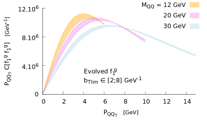
As said, after integration over the azimuthal angle $\phi_{CS}$, one gets to a good approximation $d\sigma/dq_{T}\propto q_{T}\,\mathcal{C}[f_{1}^{\,g}f_{1}^{\,g}]$. In Fig. 3 (a) we compare $q_{T}\,\mathcal{C}[f_{1}^{\,g}f_{1}^{\,g}]$ evaluated using the non-evolved Gaussian TMD model of Lansberg:2017dzg with the evolved TMD computed along the lines described in the previous section for $M_{{\cal Q}{\cal Q}}$ = 8 GeV using the range of $b_{T\lim}$ between 2 and 8 GeV^-1. The main difference one can observe is the broadening of the $\boldsymbol{P}_{{\cal Q}{\cal Q}{\scriptscriptstyle T}}$-spectrum when including evolution effects. The curves are given as functions of $\boldsymbol{P}_{{\cal Q}{\cal Q}{\scriptscriptstyle T}}$ in the range from 0 up to $M_{{\cal Q}{\cal Q}}$/2, to be in the validity range of TMD factorization.

(a)

(b)

Figure 3: (a) The normalised $\boldsymbol{P}_{{\cal Q}{\cal Q}{\scriptscriptstyle T}}$-spectrum for $J/\psi$-pair production at $M_{\psi\psi}$ = 8 GeV using two gluon TMDs. The first is a Gaussian Ansatz with $\langle k_{T}^{\,2}\rangle=3.3\pm 0.8$ GeV² obtained from the LHCb data Lansberg:2017dzg (the red curve shows the central value and the gray band the associated uncertainty). The second is the result of our present study with TMD evolution. The green band results from the uncertainty on the $b_{T}$-width of the nonperturbative Sudakov factor $S_{{\rm NP}}$. The estimated DPS contribution has been subtracted from the LHCb data (black crosses) which were also normalized over the interval. (b) The $\boldsymbol{P}_{{\cal Q}{\cal Q}{\scriptscriptstyle T}}$-spectrum using our evolved gluon TMDs at $M_{{\cal Q}{\cal Q}}$ = 12, 20 and 30 GeV for the same uncertainty on the $b_{T}$-width.

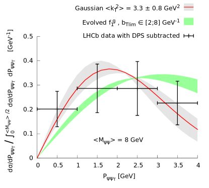
The momentum fractions of the initial gluons, $x_{1}$ and $x_{2}$, are both fixed to 10^-3. Varying the momentum fractions does not have any significant impact on the shape of the $\boldsymbol{P}_{{\cal Q}{\cal Q}{\scriptscriptstyle T}}$-spectrum or the azimuthal asymmetries. The size of the asymmetries varies by a few percent with $x$. As such variations do not change the conclusions of our analysis, we will keep the values $x_{1}=x_{2}=10^{-3}$ throughout this paper. This is also convenient for an experimental study, as a binning of the data in $Y_{{\cal Q}{\cal Q}}$ is not necessary to be able to compare them with predictions.

In Fig. 3 (b), we show evolved results for $M_{{\cal Q}{\cal Q}}$ = 12, 20 and 30 GeV within the same $b_{T\lim}$ range as Fig. 3 (b). The broadening of the $\boldsymbol{P}_{{\cal Q}{\cal Q}{\scriptscriptstyle T}}$-spectrum for increasing $M_{{\cal Q}{\cal Q}}$ is then explicit.

The azimuthal asymmetries presented in Eq. (2.3) depend on a rather complex ratio of TMD convolutions and hard-scattering coefficients. In the case of $J/\psi$-pair production, these expressions simplify for several reasons. The first one, already mentioned previously, is that because $F_{2}$ is small, the denominator can be approximated to be $F_{1}\mathcal{C}\Big{[}f_{1}^{\,g}f_{1}^{\,g}\Big{]}$. Moreover, because of the symmetry of the final state, one finds the coefficients $F_{3}$ and $F_{3}^{\prime}$ to be equal, simplifying the numerator of $\langle\cos(2\phi_{CS})\rangle$ to be $F_{3}\Big{(}\mathcal{C}\Big{[}w_{3}\,f_{1}^{\,g}h_{1}^{\perp\,g}\Big{]}+\mathcal{C}\Big{[}w_{3}^{\prime}\,h_{1}^{\perp\,g}f_{1}^{\,g}\Big{]}\Big{)}$. Finally, when one takes the initial-parton-momentum fractions to be equal, i.e. $x_{1}=x_{2}$, these two convolutions become equal as well. Since the $\boldsymbol{P}_{{\cal Q}{\cal Q}{\scriptscriptstyle T}}$-dependence of the cross-section is contained inside the convolutions, the $\boldsymbol{P}_{{\cal Q}{\cal Q}{\scriptscriptstyle T}}$-dependence of the asymmetries can be studied via the convolution ratios $\mathcal{C}\Big{[}w_{3}\,f_{1}^{\,g}h_{1}^{\perp\,g}\Big{]}/\mathcal{C}\Big{[}f_{1}^{\,g}f_{1}^{\,g}\Big{]}$ and $\mathcal{C}\Big{[}w_{4}\,h_{1}^{\perp\,g}h_{1}^{\perp\,g}\Big{]}/\mathcal{C}\Big{[}f_{1}^{\,g}f_{1}^{\,g}\Big{]}$ for $\langle\cos(2\phi_{CS})\rangle$ and $\langle\cos(4\phi_{CS})\rangle$, respectively.

The difference between both convolutions depends on the kind of TMDs they contain, but also the type of Bessel function generated by the angular integral and the weights. Because $\tilde{h}_{1}^{\perp\,g}$ is of order $\alpha_{s}$, it is naturally suppressed in comparison to $f_{1}^{\,g}$. Moreover, $\alpha_{s}(\mu_{b})$ is growing with $b_{T}$ (up to its bound $\alpha_{s}(b_{0}/b_{T\max})$) and $\tilde{h}_{1}^{\perp\,g}$ is also broader in $b_{T}$ than $f_{1}^{\,g}$. The presence of $\tilde{h}_{1}^{\perp\,g}$ in a given convolution therefore contributes to reduce the magnitude of the integrand, and to its $b_{T}$-broadening. These effects contribute to strongly suppress $\mathcal{C}\Big{[}w_{2}\,h_{1}^{\perp\,g}h_{1}^{\perp\,g}\Big{]}$with respect to $\mathcal{C}\Big{[}f_{1}^{\,g}f_{1}^{\,g}\Big{]}$. $\mathcal{C}\Big{[}w_{2}\,h_{1}^{\perp\,g}h_{1}^{\perp\,g}\Big{]}$ is of order $\alpha_{s}^{2}$ and its integrand is significantly broadened in $b_{T}$, meaning it falls faster than $\mathcal{C}\Big{[}f_{1}^{\,g}f_{1}^{\,g}\Big{]}$with increasing $\boldsymbol{P}_{{\cal Q}{\cal Q}{\scriptscriptstyle T}}$. Indeed, as a consequence of the $b_{T}$-broadening, more oscillations of the $J_{0}$ Bessel function occur in the integrand of $\mathcal{C}\Big{[}w_{2}\,h_{1}^{\perp\,g}h_{1}^{\perp\,g}\Big{]}$ than of $\mathcal{C}\Big{[}f_{1}^{\,g}f_{1}^{\,g}\Big{]}$, before being dampened by the Sudakov factors at large $b_{T}$. Each additional oscillation in the integrand brings the convolution value closer to zero. More oscillations are packed in a given $b_{T}$-range when $\boldsymbol{P}_{{\cal Q}{\cal Q}{\scriptscriptstyle T}}$ increases, widening the gap between the two convolutions, and effectively making the ratio fall with $\boldsymbol{P}_{{\cal Q}{\cal Q}{\scriptscriptstyle T}}$. This additional effect renders the $F_{2}\,\mathcal{C}\Big{[}w_{2}\,h_{1}^{\perp\,g}h_{1}^{\perp\,g}\Big{]}$ term truly negligible in the cross-section for $J/\psi$-pair production. It also means that in other processes where the hard-scattering coefficient $F_{2}$ may be large, the convolution itself would remain relatively small at scales larger than a few GeV. Besides, its influence on the cross-section will be strongest at the smallest TM.

The situation is different for the azimuthal asymmetries, which involve convolutions in the numerator that contain either the $J_{2}$ or $J_{4}$ Bessel functions. Such functions are 0 at $b_{T}$=0 and then grow in magnitude. The consequence is that the $b_{T}$-integrals containing such functions benefit from unsuppressed intermediate $b_{T}$ values. At some point, undampened large-$b_{T}$ oscillations will bring the integral value down toward 0 in a similar way as for $\mathcal{C}\Big{[}f_{1}^{\,g}f_{1}^{\,g}\Big{]}$ and $\mathcal{C}\Big{[}w_{2}\,h_{1}^{\perp\,g}h_{1}^{\perp\,g}\Big{]}$. Therefore, the $\mathcal{C}\Big{[}w_{3}\,f_{1}^{\,g}h_{1}^{\perp\,g}\Big{]}$ and $\mathcal{C}\Big{[}w_{4}\,h_{1}^{\perp\,g}h_{1}^{\perp\,g}\Big{]}$ convolutions first grow with $\boldsymbol{P}_{{\cal Q}{\cal Q}{\scriptscriptstyle T}}$ up to a peak maximum, and then decrease in value like $\mathcal{C}\Big{[}f_{1}^{\,g}f_{1}^{\,g}\Big{]}$ does. Another crucial difference is that the envelopes of $J_{2}$ and $J_{4}$ tend slower toward 0 than the $J_{0}$ one with increasing $b_{T}$. The consequence is that $\mathcal{C}\Big{[}w_{3}\,f_{1}^{\,g}h_{1}^{\perp\,g}\Big{]}$ and $\mathcal{C}\Big{[}w_{4}\,h_{1}^{\perp\,g}h_{1}^{\perp\,g}\Big{]}$ fall slower than $\mathcal{C}\Big{[}f_{1}^{\,g}f_{1}^{\,g}\Big{]}$ with $\boldsymbol{P}_{{\cal Q}{\cal Q}{\scriptscriptstyle T}}$. Hence the convolution ratios, and the azimuthal asymmetries, always grow with $\boldsymbol{P}_{{\cal Q}{\cal Q}{\scriptscriptstyle T}}$, as can be seen in Fig. 4. In addition, as the large $b_{T}$ values are less suppressed than in $\mathcal{C}\Big{[}f_{1}^{\,g}f_{1}^{\,g}\Big{]}$, the azimuthal asymmetries are also more sensitive to the variations of the nonperturbative Sudakov $S_{{\rm NP}}$. The effect is more pronounced for $\mathcal{C}\Big{[}w_{4}\,h_{1}^{\perp\,g}h_{1}^{\perp\,g}\Big{]}$ since it contains $\tilde{h}_{1}^{\perp\,g}$ twice and a broader Bessel function.

(a)

(b)

(c)

(d)

Figure 4: The azimuthal asymmetries for di-$J/\psi$ production as functions of $\boldsymbol{P}_{{\cal Q}{\cal Q}{\scriptscriptstyle T}}$. The different plots show $2\langle\cos(2\phi_{CS})\rangle$ (a,b) and $2\langle\cos(4\phi_{CS})\rangle$ (c,d), at $|\cos(\theta_{CS})|<0.25$ (a,c) and at $0.25<|\cos(\theta_{CS})|<0.5$ (b,d). Results are presented for $M_{\psi\psi}$ = 12, 21 and 30 GeV, and for $b_{T\lim}$ = 2, 4 and 8 GeV^-1.

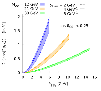
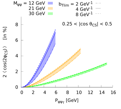
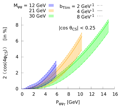
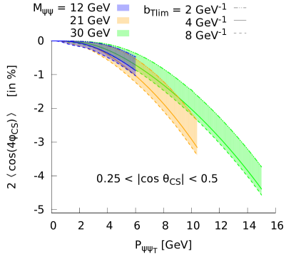
Fig. 4b displays the $\cos(2\phi_{CS})$ asymmetry as a function of $\boldsymbol{P}_{{\cal Q}{\cal Q}{\scriptscriptstyle T}}$ in the forward single $J/\psi$ rapidity region (larger $\cos(\theta_{CS})$) while 4c displays the $\cos(4\phi_{CS})$ asymmetry in the central rapidity region (small $\cos(\theta_{CS})$ with $x_{1}\simeq x_{2}$). Such choices maximize the size of the asymmetries as the associated hard-scattering coefficients are larger in these regions, without modifying the shapes of the asymmetries in $\boldsymbol{P}_{{\cal Q}{\cal Q}{\scriptscriptstyle T}}$ (see Lansberg:2017dzg for a comparison between the two rapidity regions for each asymmetry). The uncertainty band associated with the width of $S_{{\rm NP}}$ narrows with increasing $M_{{\cal Q}{\cal Q}}$ as in Fig. 3; the uncertainty remains larger for $\langle\cos(4\phi_{CS})\rangle$ as $\mathcal{C}\Big{[}w_{4}\,h_{1}^{\perp\,g}h_{1}^{\perp\,g}\Big{]}$ is more affected by $S_{{\rm NP}}$. The curves for $b_{T\lim}$ = 8 GeV^-1 (large dashes) are quite close to the ones using $b_{T\lim}$ = 4 GeV^-1 (solid line). Indeed, when $S_{{\rm NP}}$ is already significantly wider than $S_{A}$, an additional increase in its width will not affect the asymmetries anymore. Both convolutions in the ratios are larger with a wide nonperturbative Sudakov factor, yet this benefits the numerator $\Big{(}\mathcal{C}\Big{[}w_{3}\,f_{1}^{\,g}h_{1}^{\perp\,g}\Big{]}$ or $\mathcal{C}\Big{[}w_{4}\,h_{1}^{\perp\,g}h_{1}^{\perp\,g}\Big{]}\Big{)}$ more than the denominator $\Big{(}\mathcal{C}\Big{[}f_{1}^{\,g}f_{1}^{\,g}\Big{]}\Big{)}$, and the asymmetries are of a greater size for a wider $S_{{\rm NP}}$.

(a)

(b)

(c)

(d)

Figure 5: The azimuthal asymmetries for di-$J/\psi$ production as functions of $M_{\psi\psi}$. The different plots show $2\langle\cos(2\phi_{CS})\rangle$ (a,b) and $2\langle\cos(4\phi_{CS})\rangle$ (c,d), at $|\cos(\theta_{CS})|<0.25$ (a,c) and at $0.25<|\cos(\theta_{CS})|<0.5$ (b,d). Results are presented for $\boldsymbol{P}_{{\cal Q}{\cal Q}{\scriptscriptstyle T}}$ = 4, 7 and 10 GeV, and for $b_{T\lim}$ = 2, 4 and 8 GeV^-1.

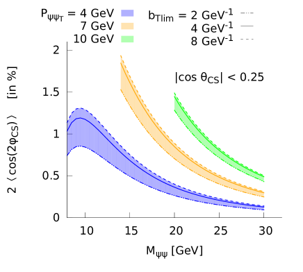
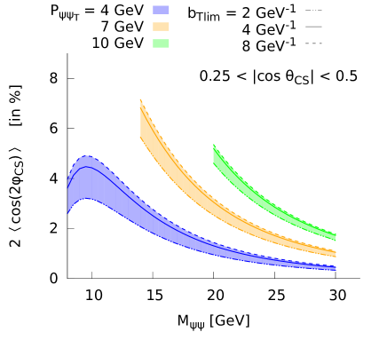
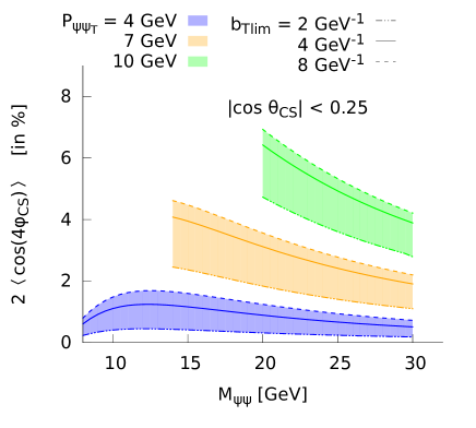
We recall that the size of the asymmetries is also influenced by the ratio of the hard-scattering coefficients which are $M_{{\cal Q}{\cal Q}}$-dependent. $F_{3}/F_{1}$ peaks around $M_{{\cal Q}{\cal Q}}$ = 12 GeV which explains why the $\cos(2\phi_{CS})$ asymmetry is largest near this value. As discussed in Lansberg:2017dzg , the ratio $F_{4}/F_{1}$ keeps growing with $M_{{\cal Q}{\cal Q}}$, approaching 1 at sufficiently large values. Yet the $\cos(4\phi_{CS})$ asymmetry gets smaller with larger $M_{{\cal Q}{\cal Q}}$. This can be better seen in Fig. 5 which depicts the same asymmetries as functions of $M_{{\cal Q}{\cal Q}}=M_{\psi\psi}$.

One first observes that, at large $M_{{\cal Q}{\cal Q}}$, the growth of the asymmetries with $\boldsymbol{P}_{{\cal Q}{\cal Q}{\scriptscriptstyle T}}$ is slower. Indeed, in such a situation, the Sudakov factors broaden the $\boldsymbol{P}_{{\cal Q}{\cal Q}{\scriptscriptstyle T}}$-shapes of the convolutions, hence the ratio varies slower. This slower increase is compensated by the fact that larger values of $M_{{\cal Q}{\cal Q}}$ allow for an extended growth of the asymmetry over a greater $\boldsymbol{P}_{{\cal Q}{\cal Q}{\scriptscriptstyle T}}$-range of validity for the TMD formalism. Secondly, the convolution ratios at a fixed value of $\boldsymbol{P}_{{\cal Q}{\cal Q}{\scriptscriptstyle T}}$ also evolve with $M_{{\cal Q}{\cal Q}}$. The computable $M_{{\cal Q}{\cal Q}}$-dependence is encoded in the perturbative Sudakov factor $S_{A}$, while $S_{{\rm NP}}$ is also logarithmically varying with $M_{{\cal Q}{\cal Q}}$ Collins:1981va . Both $S_{A}$ and $S_{{\rm NP}}$ get narrower in $b_{T}$ with increasing $M_{{\cal Q}{\cal Q}}$, leading to a decrease of the value of the convolutions. $\mathcal{C}\Big{[}w_{3}\,f_{1}^{\,g}h_{1}^{\perp\,g}\Big{]}$ and $\mathcal{C}\Big{[}w_{4}\,h_{1}^{\perp\,g}h_{1}^{\perp\,g}\Big{]}$ are more sensitive to the large $b_{T}$-value dampening and therefore fall faster with $M_{{\cal Q}{\cal Q}}$ than $\mathcal{C}\Big{[}f_{1}^{\,g}f_{1}^{\,g}\Big{]}$. This results in decreasing convolution ratios, with a steeper fall for $\mathcal{C}\Big{[}w_{4}\,h_{1}^{\perp\,g}h_{1}^{\perp\,g}\Big{]}$. However the azimuthal asymmetries also depend on the evolution with $M_{{\cal Q}{\cal Q}}$ of the hard-scattering coefficients ratios. Since $F_{4}/F_{1}$ keeps growing while $F_{3}/F_{1}$ falls after peaking at $M_{{\cal Q}{\cal Q}}\simeq$ 12 GeV, $\langle\cos(4\phi_{CS})\rangle$ will actually decrease slower than $\langle\cos(2\phi_{CS})\rangle$.

The large variations of the width of $S_{{\rm NP}}$ generate moderate uncertainties on the size of the asymmetries. The latter, although consequently smaller than when computed in a bound-saturating model Lansberg:2017dzg , still reach reasonable sizes, up to 5%-10%. We used the same nonperturbative Sudakov factor for all TMD convolutions in these computations, but the $M_{{\cal Q}{\cal Q}}$-independent part is actually expected to be non-universal. We checked that individually changing the width of $S_{{\rm NP}}$ within the $b_{T\lim}$-ranges used in this study inside the different types of convolutions, does not bring any significant modification on the observables.

So far, there are still no experimental data allowing for an extraction of the gluon TMDs inside unpolarized protons. We believe that the numerous $J/\psi$-pair-production events recorded at the LHC can give us access to information about the nonperturbative components of $f_{1}^{\,g}$ and $h_{1}^{\perp\,g}$, provided the events are selected with kinematics within the validity range of TMD factorization, $\boldsymbol{P}_{{\cal Q}{\cal Q}{\scriptscriptstyle T}}<M_{{\cal Q}{\cal Q}}/2$.

4.2 $\Upsilon$-pair production

It is also of interest to look at $\Upsilon$-pair production. The partonic subprocess is identical to that of di-$J/\psi$ production. In the non-relativistic limit, where $M_{\Upsilon}=2m_{b}$, the main difference comes from the mass of the heavy quark. We note that the value of the non-relativistic wave function at the origin (or equivalently the NRQCD LDME for the CS transition) also differs but cancels in the ratios which we consider. The feed-down pattern is also clearly different. However, as announced, we will neglect the resulting (small) feed-down effects.

Owing to this larger mass, such a process probes the evolution at generally higher scales. The coupling constant $\alpha_{s}$ is also smaller which increases the precision of the perturbative expansion. Higher scales also mean that the process is less sensitive to the (large $b_{T}$) nonperturbative behavior of the gluon TMDs. Hence, it is also less affected by the uncertainties associated with this unconstrained component.

On the experimental side, $\Upsilon$-pair production is admittedly a rare process. Yet, it starts to be accessible at the LHC. The first analysis by the CMS collaboration at $\sqrt{s}$ = 8 TeV only comprised a 40-event sample Khachatryan:2016ydm but a second one is forthcoming. During the future high luminosity LHC runs, it will definitely be possible to record a sufficient number of events for a TMD analysis of both the $\boldsymbol{P}_{{\cal Q}{\cal Q}{\scriptscriptstyle T}}$ and azimuthal dependences of the yield. Fig. 6 depicts the azimuthal modulations for $\Upsilon$-pair production as functions of $\boldsymbol{P}_{{\cal Q}{\cal Q}{\scriptscriptstyle T}}$ up to $M_{{\cal Q}{\cal Q}}/2$, for values of $M_{{\cal Q}{\cal Q}}$ of 30, 40 and 50 GeV.

(a)

(b)

(c)

(d)

Figure 6: The azimuthal asymmetries for di-$\Upsilon$ production as functions of $\boldsymbol{P}_{{\cal Q}{\cal Q}{\scriptscriptstyle T}}$. The different plots show $2\langle\cos(2\phi_{CS})\rangle$ (top) and $2\langle\cos(4\phi_{CS})\rangle$ (bottom), at $|\cos(\theta_{CS})|<0.25$ (left) and at $0.25<|\cos(\theta_{CS})|<0.5$ (right). Results are presented for $M_{\Upsilon\Upsilon}$ = 30, 40 and 50 GeV, and for $b_{T\lim}$ = 2, 4 and 8 GeV^-1. Results for $M_{\Upsilon\Upsilon}$ = 30 GeV are not included in (d) as they are below percent level.

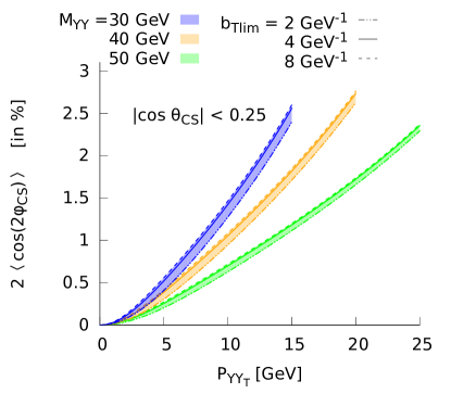
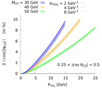
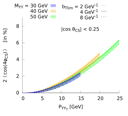
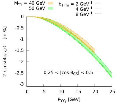
The uncertainty bands associated with the width of $S_{{\rm NP}}$ are clearly narrower than in the $J/\psi$ case. The $\cos(2\phi_{CS})$ asymmetry in Fig. 6b reaches 10% at $M_{{\cal Q}{\cal Q}}$ = 40 GeV, which is the value for which the corresponding hard-scattering coefficient ratio $F_{3}/F_{1}$ peaks for $\Upsilon$-pair production. Moreover, the decrease of the hard-scattering coefficient past the peak is slower, allowing the asymmetry to remain of similar size at $M_{{\cal Q}{\cal Q}}$ = 40 and 50 GeV.

5 Conclusions

In this paper we discussed the potential of double $J/\psi$ and $\Upsilon$ production for the study of the gluon TMDs inside unpolarized protons at the LHC. We presented the advantages of quarkonia as probes of these TMDs. We improved on previous results Lansberg:2017dzg by including TMD evolution effects, rendering the results more realistic and effectively taking into account QCD corrections that describe the evolution with the invariant mass $M_{{\cal Q}{\cal Q}}$ of the quarkonium pair. We used a simple $b_{T}$-Gaussian of variable width to parametrize the nonperturbative Sudakov factor $S_{{\rm NP}}$ in order to estimate how important its impact is on the predicted yield and asymmetries, as it currently remains unconstrained in the gluon case.

We discussed the broadening of the $\boldsymbol{P}_{{\cal Q}{\cal Q}{\scriptscriptstyle T}}$-spectrum due to the evolution in the case of double-$J/\psi$ production, as well as the uncertainty associated with a variation of the width of $S_{{\rm NP}}$ between 2 and 8 GeV^-1. As expected, we found that its influence decreases at large $M_{{\cal Q}{\cal Q}}$ as the perturbative component of the TMDs becomes dominant. We also computed the $\langle\cos(2,\!4\phi_{CS})\rangle$ asymmetries as functions of $\boldsymbol{P}_{{\cal Q}{\cal Q}{\scriptscriptstyle T}}$ and $M_{{\cal Q}{\cal Q}}$. We found a notable suppression of the asymmetries in comparison to Lansberg:2017dzg , caused by the fact that $h_{1}^{\perp\,g}$ appears at order $\alpha_{s}$ in the evolution formalism. We nevertheless found that such asymmetries still reach reasonable sizes for larger $\boldsymbol{P}_{{\cal Q}{\cal Q}{\scriptscriptstyle T}}$ values and could be observed in the events already collected and to be recorded in the future. We found that the size of the asymmetries increases with $\boldsymbol{P}_{{\cal Q}{\cal Q}{\scriptscriptstyle T}}$. Such a behavior is explained by the relative slower fall in $\boldsymbol{P}_{{\cal Q}{\cal Q}{\scriptscriptstyle T}}$ of the TMD convolutions containing $h_{1}^{\perp\,g}$.

TMD factorization needs to be matched onto its collinear counterpart when $\boldsymbol{P}_{{\cal Q}{\cal Q}{\scriptscriptstyle T}}$ approaches $M_{{\cal Q}{\cal Q}}$. Since the latter generates no asymmetries at leading twist, a $Y$-term becomes necessary at some point in order to neutralize the growth of the asymmetries and force them toward zero. We also observed that, in spite of the hard-scattering coefficient ratio $F_{4}/F_{1}$ approaching 1 at large energy, the $\cos(4\phi)$ asymmetry actually falls with $M_{{\cal Q}{\cal Q}}$.

Overall we conclude that $J/\psi$-pair production is a promising process to measure azimuthal asymmetries related to gluon TMDs as well as the effect of the evolution on the $\boldsymbol{P}_{{\cal Q}{\cal Q}{\scriptscriptstyle T}}$-spectrum. The energy threshold for this process is relatively low, making it sensitive to the nonperturbative component of the TMDs. The large event sample to be collected by the different collaborations at the LHC should give enough statistics to constrain them. $\Upsilon$-pair production presents the interesting opportunity to measure sizeable asymmetries at scales where perturbative contributions dominate, with a reduced necessity to include higher-order corrections. We also presented predictions for the asymmetries as functions of $\boldsymbol{P}_{{\cal Q}{\cal Q}{\scriptscriptstyle T}}$ for $\Upsilon$-pair production. With sufficient data to come, it would allow for a complementary extraction of the gluon TMDs, while the expected size of asymmetries remain similar. Although $\Upsilon$ pairs remain extremely rare at the LHC, the future high-luminosity runs will make it possible to acquire enough statistics.

Accessing information about the gluon TMDs can thus already be done at the LHC using quarkonium production, although more efforts in the direction of Echevarria:2019ynx are needed in order to obtain rigorous factorization theorems and expressions beyond tree level. It would give us a preview of what we can expect to find at a future Electron-Ion Collider Accardi:2012qut or fixed-target experiments at the LHC Hadjidakis:2018ifr ; Lansberg:2015lva ; Massacrier:2015qba ; Lansberg:2012kf ; Brodsky:2012vg , where these distributions should be accessible through different reactions. Because of the fundamental differences in these experimental setups, it is of great interest to measure the same TMDs using both of them, in order to be able to check fundamental predictions of the formalism such as the evolution and the universality.

References

- (1) J. P. Ralston and D. E. Soper, “Production of Dimuons from High-Energy Polarized Proton Proton Collisions,” Nucl. Phys. B152 (1979) 109.
- (2) D. W. Sivers, “Single Spin Production Asymmetries from the Hard Scattering of Point-Like Constituents,” Phys. Rev. D41 (1990) 83.
- (3) R. D. Tangerman and P. J. Mulders, “Intrinsic transverse momentum and the polarized Drell-Yan process,” Phys. Rev. D51 (1995) 3357–3372, arXiv:hep-ph/9403227 [hep-ph].
- (4) J. Collins, “Foundations of perturbative QCD,” Camb. Monogr. Part. Phys. Nucl. Phys. Cosmol. 32 (2011) 1–624.
- (5) M. G. Echevarria, A. Idilbi, and I. Scimemi, “Factorization Theorem For Drell-Yan At Low And Transverse Momentum Distributions On-The-Light-Cone,” JHEP 07 (2012) 002, arXiv:1111.4996 [hep-ph].
- (6) M. G. Echevarria, A. Idilbi, and I. Scimemi, “Soft and Collinear Factorization and Transverse Momentum Dependent Parton Distribution Functions,” Phys. Lett. B726 (2013) 795–801, arXiv:1211.1947 [hep-ph].
- (7) P. J. Mulders and J. Rodrigues, “Transverse momentum dependence in gluon distribution and fragmentation functions,” Phys. Rev. D63 (2001) 094021, arXiv:hep-ph/0009343 [hep-ph].
- (8) D. Boer, W. J. den Dunnen, C. Pisano, M. Schlegel, and W. Vogelsang, “Linearly Polarized Gluons and the Higgs Transverse Momentum Distribution,” Phys. Rev. Lett. 108 (2012) 032002, arXiv:1109.1444 [hep-ph].
- (9) P. Sun, B.-W. Xiao, and F. Yuan, “Gluon Distribution Functions and Higgs Boson Production at Moderate Transverse Momentum,” Phys. Rev. D84 (2011) 094005, arXiv:1109.1354 [hep-ph].
- (10) J.-W. Qiu, M. Schlegel, and W. Vogelsang, “Probing Gluonic Spin-Orbit Correlations in Photon Pair Production,” Phys. Rev. Lett. 107 (2011) 062001, arXiv:1103.3861 [hep-ph].
- (11) R. M. Godbole, A. Misra, A. Mukherjee, and V. S. Rawoot, “Sivers Effect and Transverse Single Spin Asymmetry in ,” Phys. Rev. D85 (2012) 094013, arXiv:1201.1066 [hep-ph].
- (12) D. Boer and C. Pisano, “Polarized gluon studies with charmonium and bottomonium at LHCb and AFTER,” Phys. Rev. D86 (2012) 094007, arXiv:1208.3642 [hep-ph].
- (13) R. M. Godbole, A. Misra, A. Mukherjee, and V. S. Rawoot, “Transverse Single Spin Asymmetry in and Transverse Momentum Dependent Evolution of the Sivers Function,” Phys. Rev. D88 no. 1, (2013) 014029, arXiv:1304.2584 [hep-ph].
- (14) R. M. Godbole, A. Kaushik, A. Misra, and V. S. Rawoot, “Transverse single spin asymmetry in and evolution of Sivers function-II,” Phys. Rev. D91 no. 1, (2015) 014005, arXiv:1405.3560 [hep-ph].
- (15) G.-P. Zhang, “Probing transverse momentum dependent gluon distribution functions from hadronic quarkonium pair production,” Phys. Rev. D90 no. 9, (2014) 094011, arXiv:1406.5476 [hep-ph].
- (16) D. Boer and C. Pisano, “Impact of gluon polarization on Higgs boson plus jet production at the LHC,” Phys. Rev. D91 no. 7, (2015) 074024, arXiv:1412.5556 [hep-ph].
- (17) W. J. den Dunnen, J. P. Lansberg, C. Pisano, and M. Schlegel, “Accessing the Transverse Dynamics and Polarization of Gluons inside the Proton at the LHC,” Phys. Rev. Lett. 112 (2014) 212001, arXiv:1401.7611 [hep-ph].
- (18) D. Boer and W. J. den Dunnen, “TMD evolution and the Higgs transverse momentum distribution,” Nucl. Phys. B886 (2014) 421–435, arXiv:1404.6753 [hep-ph].
- (19) G.-P. Zhang, “Transverse momentum dependent gluon fragmentation functions from production at colliders,” Eur. Phys. J. C75 no. 10, (2015) 503, arXiv:1504.06699 [hep-ph].
- (20) A. Mukherjee and S. Rajesh, “Probing Transverse Momentum Dependent Parton Distributions in Charmonium and Bottomonium Production,” Phys. Rev. D93 no. 5, (2016) 054018, arXiv:1511.04319 [hep-ph].
- (21) M. G. Echevarria, T. Kasemets, P. J. Mulders, and C. Pisano, “QCD evolution of (un)polarized gluon TMDPDFs and the Higgs -distribution,” JHEP 07 (2015) 158, arXiv:1502.05354 [hep-ph]. [Erratum: JHEP05,073(2017)].
- (22) A. Mukherjee and S. Rajesh, “ production in polarized and unpolarized ep collision and Sivers and asymmetries,” Eur. Phys. J. C77 no. 12, (2017) 854, arXiv:1609.05596 [hep-ph].
- (23) A. Mukherjee and S. Rajesh, “Linearly polarized gluons in charmonium and bottomonium production in color octet model,” Phys. Rev. D95 no. 3, (2017) 034039, arXiv:1611.05974 [hep-ph].
- (24) D. Boer, “Gluon TMDs in quarkonium production,” Few Body Syst. 58 no. 2, (2017) 32, arXiv:1611.06089 [hep-ph].
- (25) J.-P. Lansberg, C. Pisano, and M. Schlegel, “Associated production of a dilepton and a at the LHC as a probe of gluon transverse momentum dependent distributions,” Nucl. Phys. B920 (2017) 192–210, arXiv:1702.00305 [hep-ph].
- (26) R. M. Godbole, A. Kaushik, A. Misra, V. Rawoot, and B. Sonawane, “Transverse single spin asymmetry in ,” Phys. Rev. D96 no. 9, (2017) 096025, arXiv:1703.01991 [hep-ph].
- (27) U. D’Alesio, F. Murgia, C. Pisano, and P. Taels, “Probing the gluon Sivers function in and ,” Phys. Rev. D96 no. 3, (2017) 036011, arXiv:1705.04169 [hep-ph].
- (28) S. Rajesh, R. Kishore, and A. Mukherjee, “Sivers effect in Inelastic Photoproduction in Collision in Color Octet Model,” Phys. Rev. D98 no. 1, (2018) 014007, arXiv:1802.10359 [hep-ph].
- (29) A. Bacchetta, D. Boer, C. Pisano, and P. Taels, “Gluon TMDs and NRQCD matrix elements in production at an EIC,” arXiv:1809.02056 [hep-ph].
- (30) J.-P. Lansberg, C. Pisano, F. Scarpa, and M. Schlegel, “Pinning down the linearly-polarised gluons inside unpolarised protons using quarkonium-pair production at the LHC,” Phys. Lett. B784 (2018) 217–222, arXiv:1710.01684 [hep-ph]. [Erratum: Phys. Lett.B791,420(2019)].
- (31) R. Kishore and A. Mukherjee, “Accessing linearly polarized gluon distribution in production at the electron-ion collider,” Phys. Rev. D99 no. 5, (2019) 054012, arXiv:1811.07495 [hep-ph].
- (32) P. Sun, C. P. Yuan, and F. Yuan, “Heavy Quarkonium Production at Low Pt in NRQCD with Soft Gluon Resummation,” Phys. Rev. D88 (2013) 054008, arXiv:1210.3432 [hep-ph].
- (33) J. P. Ma, J. X. Wang, and S. Zhao, “Transverse momentum dependent factorization for quarkonium production at low transverse momentum,” Phys. Rev. D88 no. 1, (2013) 014027, arXiv:1211.7144 [hep-ph].
- (34) J. P. Ma, J. X. Wang, and S. Zhao, “Breakdown of QCD Factorization for P-Wave Quarkonium Production at Low Transverse Momentum,” Phys. Lett. B737 (2014) 103–108, arXiv:1405.3373 [hep-ph].
- (35) J. P. Ma and C. Wang, “QCD factorization for quarkonium production in hadron collisions at low transverse momentum,” Phys. Rev. D93 no. 1, (2016) 014025, arXiv:1509.04421 [hep-ph].
- (36) J.-P. Lansberg, “New Observables in Inclusive Production of Quarkonia,” arXiv:1903.09185 [hep-ph].
- (37) J. Collins and J.-W. Qiu, “ factorization is violated in production of high-transverse-momentum particles in hadron-hadron collisions,” Phys. Rev. D75 (2007) 114014, arXiv:0705.2141 [hep-ph].
- (38) J. Collins, “2-soft-gluon exchange and factorization breaking,” arXiv:0708.4410 [hep-ph].
- (39) T. C. Rogers and P. J. Mulders, “No Generalized TMD-Factorization in Hadro-Production of High Transverse Momentum Hadrons,” Phys. Rev. D81 (2010) 094006, arXiv:1001.2977 [hep-ph].
- (40) D0 Collaboration, V. M. Abazov et al., “Observation and Studies of Double Production at the Tevatron,” Phys. Rev. D90 no. 11, (2014) 111101, arXiv:1406.2380 [hep-ex].
- (41) CMS Collaboration, V. Khachatryan et al., “Measurement of prompt pair production in pp collisions at = 7 Tev,” JHEP 09 (2014) 094, arXiv:1406.0484 [hep-ex].
- (42) LHCb Collaboration, R. Aaij et al., “Observation of pair production in collisions at ,” Phys. Lett. B707 (2012) 52–59, arXiv:1109.0963 [hep-ex].
- (43) LHCb Collaboration, R. Aaij et al., “Measurement of the J/ pair production cross-section in pp collisions at TeV,” JHEP 06 (2017) 047, arXiv:1612.07451 [hep-ex]. [Erratum: JHEP10,068(2017)].
- (44) ATLAS Collaboration, M. Aaboud et al., “Measurement of the prompt J/ pair production cross-section in pp collisions at TeV with the ATLAS detector,” Eur. Phys. J. C77 no. 2, (2017) 76, arXiv:1612.02950 [hep-ex].
- (45) J. Collins, “New definition of TMD parton densities,” Int. J. Mod. Phys. Conf. Ser. 4 (2011) 85–96, arXiv:1107.4123 [hep-ph].
- (46) M. G. Echevarria, A. Idilbi, A. Schaefer, and I. Scimemi, “Model-Independent Evolution of Transverse Momentum Dependent Distribution Functions (TMDs) at NNLL,” Eur. Phys. J. C73 no. 12, (2013) 2636, arXiv:1208.1281 [hep-ph].
- (47) M. G. Echevarria, A. Idilbi, and I. Scimemi, “Unified treatment of the QCD evolution of all (un-)polarized transverse momentum dependent functions: Collins function as a study case,” Phys. Rev. D90 no. 1, (2014) 014003, arXiv:1402.0869 [hep-ph].
- (48) M. G. Echevarria, “Proper TMD factorization for quarkonia production: as a study case,” arXiv:1907.06494 [hep-ph].
- (49) S. Meissner, A. Metz, and K. Goeke, “Relations between generalized and transverse momentum dependent parton distributions,” Phys. Rev. D76 (2007) 034002, arXiv:hep-ph/0703176 [HEP-PH].
- (50) D. Boer, S. Cotogno, T. van Daal, P. J. Mulders, A. Signori, and Y.-J. Zhou, “Gluon and Wilson loop TMDs for hadrons of spin 1,” JHEP 10 (2016) 013, arXiv:1607.01654 [hep-ph].
- (51) C.-F. Qiao, L.-P. Sun, and P. Sun, “Testing Charmonium Production Mechamism via Polarized J/psi Pair Production at the LHC,” J. Phys. G37 (2010) 075019, arXiv:0903.0954 [hep-ph].
- (52) V. G. Kartvelishvili and S. M. Esakiya, “On hadronic production of pairs of J/psi mesons.,” Soviet Journal of Nuclear Physics 38(3) (1983) 430–432.
- (53) B. Humpert and P. Mery, “Psi psi production at collider energies,” Z. Phys. C20 (1983) 83.
- (54) C.-H. Chang, “Hadronic Production of Associated With a Gluon,” Nucl. Phys. B172 (1980) 425–434.
- (55) R. Baier and R. Ruckl, “Hadronic Production of J/psi and Upsilon: Transverse Momentum Distributions,” Phys. Lett. 102B (1981) 364–370.
- (56) R. Baier and R. Ruckl, “Hadronic Collisions: A Quarkonium Factory,” Z. Phys. C19 (1983) 251.
- (57) G. T. Bodwin, E. Braaten, and G. P. Lepage, “Rigorous QCD analysis of inclusive annihilation and production of heavy quarkonium,” Phys. Rev. D51 (1995) 1125–1171, arXiv:hep-ph/9407339 [hep-ph]. [Erratum: Phys. Rev.D55,5853(1997)].
- (58) P. L. Cho and A. K. Leibovich, “Color octet quarkonia production. 2.,” Phys. Rev. D53 (1996) 6203–6217, arXiv:hep-ph/9511315 [hep-ph].
- (59) P. L. Cho and A. K. Leibovich, “Color octet quarkonia production,” Phys. Rev. D53 (1996) 150–162, arXiv:hep-ph/9505329 [hep-ph].
- (60) A. Andronic et al., “Heavy-flavour and quarkonium production in the LHC era: from proton–proton to heavy-ion collisions,” Eur. Phys. J. C76 no. 3, (2016) 107, arXiv:1506.03981 [nucl-ex].
- (61) N. Brambilla et al., “Heavy Quarkonium: Progress, Puzzles, and Opportunities,” Eur. Phys. J. C71 (2011) 1534, arXiv:1010.5827 [hep-ph].
- (62) J. P. Lansberg, “, ’ and production at hadron colliders: A Review,” Int. J. Mod. Phys. A21 (2006) 3857–3916, arXiv:hep-ph/0602091 [hep-ph].
- (63) P. Ko, C. Yu, and J. Lee, “Inclusive double-quarkonium production at the Large Hadron Collider,” JHEP 01 (2011) 070, arXiv:1007.3095 [hep-ph].
- (64) Y.-J. Li, G.-Z. Xu, K.-Y. Liu, and Y.-J. Zhang, “Relativistic Correction to J/psi and Upsilon Pair Production,” JHEP 07 (2013) 051, arXiv:1303.1383 [hep-ph].
- (65) J.-P. Lansberg and H.-S. Shao, “-pair production at large momenta: Indications for double parton scatterings and large contributions,” Phys. Lett. B751 (2015) 479–486, arXiv:1410.8822 [hep-ph].
- (66) Z.-G. He and B. A. Kniehl, “Complete Nonrelativistic-QCD Prediction for Prompt Double J/psi Hadroproduction,” Phys. Rev. Lett. 115 no. 2, (2015) 022002, arXiv:1609.02786 [hep-ph].
- (67) J.-P. Lansberg, H.-S. Shao, N. Yamanaka, and Y.-J. Zhang, “Prompt -pair production at the LHC: impact of loop-induced contributions and of the colour-octet mechanism,” arXiv:1906.10049 [hep-ph].
- (68) M. G. Echevarria, T. Kasemets, J.-P. Lansberg, C. Pisano, and A. Signori, “Matching factorization theorems with an inverse-error weighting,” Phys. Lett. B781 (2018) 161–168, arXiv:1801.01480 [hep-ph].
- (69) J.-P. Lansberg and H.-S. Shao, “Production of versus at the LHC: Importance of Real Corrections,” Phys. Rev. Lett. 111 (2013) 122001, arXiv:1308.0474 [hep-ph].
- (70) L.-P. Sun, H. Han, and K.-T. Chao, “Impact of pair production at the LHC and predictions in nonrelativistic QCD,” Phys. Rev. D94 no. 7, (2016) 074033, arXiv:1404.4042 [hep-ph].
- (71) A. K. Likhoded, A. V. Luchinsky, and S. V. Poslavsky, “Production of and with real gluon emission at LHC,” Phys. Rev. D94 no. 5, (2016) 054017, arXiv:1606.06767 [hep-ph].
- (72) C. H. Kom, A. Kulesza, and W. J. Stirling, “Pair Production of J/psi as a Probe of Double Parton Scattering at LHCb,” Phys. Rev. Lett. 107 (2011) 082002, arXiv:1105.4186 [hep-ph].
- (73) M. Diehl, P. Plossl, and A. Schafer, “Proof of sum rules for double parton distributions in QCD,” Eur. Phys. J. C79 no. 3, (2019) 253, arXiv:1811.00289 [hep-ph].
- (74) M. G. A. Buffing, M. Diehl, and T. Kasemets, “Transverse momentum in double parton scattering: factorisation, evolution and matching,” JHEP 01 (2018) 044, arXiv:1708.03528 [hep-ph].
- (75) M. Diehl, J. R. Gaunt, and K. Schonwald, “Double hard scattering without double counting,” JHEP 06 (2017) 083, arXiv:1702.06486 [hep-ph].
- (76) M. Diehl and J. R. Gaunt, “Double parton scattering theory overview,” Adv. Ser. Direct. High Energy Phys. 29 (2018) 7–28, arXiv:1710.04408 [hep-ph].
- (77) Axial Field Spectrometer Collaboration, T. Åkesson et al., “Double Parton Scattering in Collisions at -GeV,” Z. Phys. C34 (1987) 163.
- (78) UA2 Collaboration, J. Alitti et al., “A Study of multi - jet events at the CERN anti-p p collider and a search for double parton scattering,” Phys. Lett. B268 (1991) 145–154.
- (79) CDF Collaboration, F. Abe et al., “Study of four jet events and evidence for double parton interactions in collisions at TeV,” Phys. Rev. D47 (1993) 4857–4871.
- (80) CDF Collaboration, F. Abe et al., “Double parton scattering in collisions at TeV,” Phys. Rev. D56 (1997) 3811–3832.
- (81) D0 Collaboration, V. M. Abazov et al., “Double parton interactions in +3 jet events in bar collisions TeV.,” Phys. Rev. D81 (2010) 052012, arXiv:0912.5104 [hep-ex].
- (82) ATLAS Collaboration, G. Aad et al., “Measurement of hard double-parton interactions in + 2 jet events at =7 TeV with the ATLAS detector,” New J. Phys. 15 (2013) 033038, arXiv:1301.6872 [hep-ex].
- (83) CMS Collaboration, S. Chatrchyan et al., “Study of double parton scattering using W + 2-jet events in proton-proton collisions at = 7 TeV,” JHEP 03 (2014) 032, arXiv:1312.5729 [hep-ex].
- (84) J.-P. Lansberg, H.-S. Shao, and N. Yamanaka, “Indication for double parton scatterings in prompt production at the LHC,” Phys. Lett. B781 (2018) 485–491, arXiv:1707.04350 [hep-ph].
- (85) A. V. Berezhnoy, A. K. Likhoded, and A. A. Novoselov, “-meson pair production at LHC,” Phys. Rev. D87 no. 5, (2013) 054023, arXiv:1210.5754 [hep-ph].
- (86) J. C. Collins and D. E. Soper, “Angular Distribution of Dileptons in High-Energy Hadron Collisions,” Phys. Rev. D16 (1977) 2219.
- (87) J. Collins, L. Gamberg, A. Prokudin, T. C. Rogers, N. Sato, and B. Wang, “Relating Transverse Momentum Dependent and Collinear Factorization Theorems in a Generalized Formalism,” Phys. Rev. D94 no. 3, (2016) 034014, arXiv:1605.00671 [hep-ph].
- (88) F. Landry, R. Brock, P. M. Nadolsky, and C. P. Yuan, “Tevatron Run-1 boson data and Collins-Soper-Sterman resummation formalism,” Phys. Rev. D67 (2003) 073016, arXiv:hep-ph/0212159 [hep-ph].
- (89) A. V. Konychev and P. M. Nadolsky, “Universality of the Collins-Soper-Sterman nonperturbative function in gauge boson production,” Phys. Lett. B633 (2006) 710–714, arXiv:hep-ph/0506225 [hep-ph].
- (90) S. M. Aybat and T. C. Rogers, “TMD Parton Distribution and Fragmentation Functions with QCD Evolution,” Phys. Rev. D83 (2011) 114042, arXiv:1101.5057 [hep-ph].
- (91) J. Collins and T. Rogers, “Understanding the large-distance behavior of transverse-momentum-dependent parton densities and the Collins-Soper evolution kernel,” Phys. Rev. D91 no. 7, (2015) 074020, arXiv:1412.3820 [hep-ph].
- (92) U. D’Alesio, M. G. Echevarria, S. Melis, and I. Scimemi, “Non-perturbative QCD effects in spectra of Drell-Yan and Z-boson production,” JHEP 11 (2014) 098, arXiv:1407.3311 [hep-ph].
- (93) J. C. Collins and D. E. Soper, “Back-To-Back Jets: Fourier Transform from B to K-Transverse,” Nucl. Phys. B197 (1982) 446–476.
- (94) CMS Collaboration, V. Khachatryan et al., “Observation of (1S) pair production in proton-proton collisions at TeV,” JHEP 05 (2017) 013, arXiv:1610.07095 [hep-ex].
- (95) A. Accardi et al., “Electron Ion Collider: The Next QCD Frontier,” Eur. Phys. J. A52 no. 9, (2016) 268, arXiv:1212.1701 [nucl-ex].
- (96) C. Hadjidakis et al., “A Fixed-Target Programme at the LHC: Physics Case and Projected Performances for Heavy-Ion, Hadron, Spin and Astroparticle Studies,” arXiv:1807.00603 [hep-ex].
- (97) J.-P. Lansberg and H.-S. Shao, “Double-quarkonium production at a fixed-target experiment at the LHC (AFTER@LHC),” Nucl. Phys. B900 (2015) 273–294, arXiv:1504.06531 [hep-ph].
- (98) L. Massacrier, B. Trzeciak, F. Fleuret, C. Hadjidakis, D. Kikola, J. P. Lansberg, and H. S. Shao, “Feasibility studies for quarkonium production at a fixed-target experiment using the LHC proton and lead beams (AFTER@LHC),” Adv. High Energy Phys. 2015 (2015) 986348, arXiv:1504.05145 [hep-ex].
- (99) J. P. Lansberg, S. J. Brodsky, F. Fleuret, and C. Hadjidakis, “Quarkonium Physics at a Fixed-Target Experiment using the LHC Beams,” Few Body Syst. 53 (2012) 11–25, arXiv:1204.5793 [hep-ph].
- (100) S. J. Brodsky, F. Fleuret, C. Hadjidakis, and J. P. Lansberg, “Physics Opportunities of a Fixed-Target Experiment using the LHC Beams,” Phys. Rept. 522 (2013) 239–255, arXiv:1202.6585 [hep-ph].