Minimizing Margin of Victory for Fair Political and Educational Districting

Abstract

In many practical scenarios, a population is divided into disjoint groups for better administration, e.g., electorates into political districts, employees into departments, students into school districts, and so on. However, grouping people arbitrarily may lead to biased partitions, raising concerns of gerrymandering in political districting, racial segregation in schools, etc. To counter such issues, in this paper, we conceptualize such problems in a voting scenario, and propose Fair Districting problem to divide a given set of people having preference over candidates into $k$ groups such that the maximum margin of victory of any group is minimized. We also propose the Fair Connected Districting problem which additionally requires each group to be connected. We show that the Fair Districting problem is $\mathsf{NP}$-complete for plurality voting even if we have only $3$ candidates but admits polynomial time algorithms if we assume $k$ to be some constant or everyone can be moved to any group. In contrast, we show that the Fair Connected Districting problem is $\mathsf{NP}$-complete for plurality voting even if we have only $2$ candidates and $k=2$. Finally, we propose heuristic algorithms for both the problems and show their effectiveness in UK political districting and in lowering racial segregation in public schools in the US.

Introduction

Dividing a population into smaller groups is often a practical necessity for better administration. For example, in many democratic countries (most notably, the countries who follow the Westminster System e.g., UK, Canada, India, Australia, or the Presidential System e.g., US, Brazil, Mexico, Indonesia), electorates are divided into electoral districts; in many organizations, employees are divided into administrative units like departments; students enrolled in public schools in the US are divided into school districts; and so on. However, the population is not homogeneous, it consists of people with different attributes – gender, race, religion, ideology, etc. Dividing people arbitrarily may lead to biased grouping, manifested differently in different contexts.

In electoral districting, given the voting pattern of the electorate, political parties in power may draw the district boundaries that favor them – a practice termed as gerrymandering (?). For example, majority of the opposition supporters may be assigned to a few districts, such that the opponents become minority in other districts. Alternatively, the ruling party may want to ensure that it enjoys a healthy lead over its opponents in many districts, so that if a handful of its supporters change sides, it does not hamper the winnability. There have been several instances of such manipulations in electoral (re)districting in the US, starting as early as in 1812, by then Massachusetts governor Elbridge Gerry (the term gerrymandering originated after him) (?).

Public schools in the US are governed by school boards representing local communities, and are largely funded from local property taxes (?; ?). Most of the students go to a school in the district they live, proximity playing an important role in the school choice (?). Thus, the way schools are distributed determines racial composition of their students and the revenue they earn. Several reports claim that wealthier, whiter communities have pushed policies so that white families can live in white-majority areas and attend white-majority schools (?; ?). Despite the desegregating efforts following the landmark Supreme Court verdict in Brown v. Board of Education case in 1954 (which ruled racial segregation of children in public schools to be unconstitutional), $63\%$ of classmates of a white student are whites, compared to $48\%$ of all students being whites; similarly, $40\%$ of black and Hispanic students attend schools where over $90\%$ students are people of color (?). As a consequence, a recent report by an educational non-profit EdBuild claimed that “Non-white school districts get $23 Billion less than white districts, despite serving the same number of students” (?).

To counter such unfairness issues while dividing people into groups, in this paper, we conceptualize such problems in a voting scenario: the goal is to divide a set of $n$ people, each having a preference over a set of candidates, into $k$ groups. While the mapping of electoral districting into voting is direct and utilizes people’s ideological preferences, we can think of context-specific mapping in other scenarios. For example, in school districting, we can think of students having preference according to their sensitive attributes (e.g., gender, race, etc.). Once the mapping is done, we propose the Fair Districting problem to create $k$ groups such that the maximum margin of victory of any group is minimized, where margin of victory is defined as the number of people who need to change their preference to change the winner. We also propose the Fair Connected Districting problem which additionally requires each group to be connected. Reducing margin of victory would lead to everyone’s opinion within a group to be valuable, since the consensus of the group can be changed even if a small number of people change their preferences. In practical applications, it would lead to higher accountability from the elected candidate in political districting, lower racial segregation in schools, increase inter-discipline exchange in academic departments, and so on.

Contribution

We make the following contributions in this paper.

• We show that the Fair Districting problem is $\mathsf{NP}$-complete for the plurality voting rule even when we have only $3$ alternatives and there is no constraint on the size of individual groups [Theorem 1]. We complement this intractability result by proving existence of polynomial time algorithms, when (i) every voter can be moved to any group (which we term as the Fair Partitioning problem) [Theorem 3], and (ii) we have a constant number of groups [Theorem 4] for the plurality voting rule.

• We show that the Fair Connected Districting problem is $\mathsf{NP}$-complete for the plurality voting rule even when there is only $2$ alternatives, $2$ districts, the maximum degree of any vertex in the underlying graph is $5$, and no constraint on the size of districts [Theorem 2]. This shows that, although both Fair Districting and Fair Connected Districting problems are $\mathsf{NP}$-complete, Fair Connected Districting problem is computationally harder than the Fair Districting problem.

• We propose heuristic algorithms for both Fair Districting and Fair Connected Districting problems and show their effectiveness in reducing margin of victory in electoral districts in the UK, as well as in lowering racial segregation in public schools in the US.

Related Work

Voting mechanisms have been at the center of historical, political, and sociological studies (?; ?; ?; ?), due to their impact on local communities and society at large. The problem of unfair distribution of voters into districts, otherwise known as gerrymandering, has received significant attention from academic researchers (?; ?; ?; ?), and in particular from the computational social choice theorists, setting geographical (?) and social constraints (?; ?; ?) to population mobility.

Central to the problem of gerrymandering is the concept of representation: does a collective represent the choices or attributes of those comprising it? In other words, does a district represent its voters? While recent papers conceptualize different measures of representation in voting scenarios (?; ?; ?; ?; ?), to our knowledge, we are the first to use the concept of margin of victory for re-districting voters to achieve better representation. While minimizing margin of victory does not ensure proportional representation of all voter choices in each district, it at least ensures that the voices present are not lost in the crowd. Intuitively, lowering margin of victory across districts would ensure a strong opposition to each majority winner, safeguarding against district monopolies, as well as against diluting voter power across many districts.

Computing the margin of victory for different voting rules has been studied in (?), while (?) and (?) estimate it in real elections. However, to our knowledge, the problem of minimizing margin of victory has not attracted much attention. In this paper, we characterize the complexity of this problem for plurality voting, one of the most common voting rules, and give practical algorithms to solve it in real and synthetic datasets.

Preliminaries

Voting Setting

For a positive integer $k$, we denote the set $\{1,2,\ldots,k\}$ by $[k]$. Let $\mathcal{A}=\{a_{i}:i\in[m]\}$ be a set of $m$ alternatives. A complete order over the set $\mathcal{A}$ of alternatives is called a preference. We denote the set of all possible preferences over $\mathcal{A}$ by $\mathcal{L}(\mathcal{A})$. A tuple $(\succ_{i})_{i\in[n]}\in\mathcal{L}(\mathcal{A})^{n}$ of $n$ preferences is called a profile. An election $\mathcal{E}$ is a tuple $(\succ,\mathcal{A})$ where $\succ$ is a profile over a set $\mathcal{A}$ of alternatives. If not mentioned otherwise, we denote the number of alternatives and the number of preferences by $m$ and $n$ respectively. A map $r:\uplus_{n,|\mathcal{A}|\in\mathbb{N}^{+}}\mathcal{L}(\mathcal{A})^{n}\longrightarrow 2^{\mathcal{A}}\setminus\{\emptyset\}$ is called a voting rule. In this paper we consider the plurality voting rule where the set of winners is the set of alternatives who appear at the first position of a highest number of alternatives. We say that a voter votes for an alternative if the voter prefers that alternative most. The number of preferences where an alternative appears at the first place is called her plurality score.

Margin of Victory

Let $r$ be any voting rule. The margin of victory of an election $((\succ_{i})_{i\in[n]},\mathcal{A})$ is the minimum number of votes that needs to be changed to change the election outcome. It easily follows that the margin of victory of a plurality election is the ceiling of half the difference between the plurality score of the two highest plurality scores of the alternatives. For ease of notation, we assume that the margin of victory of an empty election (no voters) is $\infty$.

Problem Definition

We now define our basic problem which we call Fair Districting.

Definition 1 (Fair Districting).

Given a set $\mathcal{A}$ of $m$ alternatives, a set $\mathcal{V}$ of $n$ voters along with their corresponding preferences, a set of $k$ groups $\mathcal{H}=\{H_{i},i\in[k]\}$ along with the set $\mathcal{V}_{i}$ of voters corresponding to each group $H_{i}$ for $i\in[k]$ such that $(\mathcal{V}_{i})_{i\in[k]}$ forms a partition of $\mathcal{V}$, a function $\pi:\mathcal{V}\longrightarrow 2^{\mathcal{H}}\setminus\{\emptyset\}$ denoting the set of groups where each voter can be part of, minimum size $s_{min}$ and maximum size $s_{max}$ of every group, and a target $t$ of maximum margin of victory of any group, compute if there exists a partition $(\mathcal{V}_{i}^{\prime})_{i\in[k]}$ of $\mathcal{V}$ into these $k$ groups such that the following holds.

1. For every $i\in[k]$ and $v\in\mathcal{V}_{i}^{\prime}$, we have $H_{i}\in\pi(v)$

2. For every $i\in[k]$, we have $s_{min}\leqslant|\mathcal{V}_{i}^{\prime}|\leqslant s_{max}$

3. The margin of victory in the group $H_{i}$ is at most $t$ for every $i\in[k]$

We denote an arbitrary instance of this problem by $(\mathcal{A},\mathcal{V},k,\mathcal{H}=(H_{i})_{i\in[k]},(\mathcal{V}_{i})_{i\in[k]},\pi,s_{min},s_{max},t)$.

An important special case of Fair Districting is when every voter can be moved to every district; that is $\pi(v)=\mathcal{H}$ for every voter $v\in\mathcal{V}$. We call this problem Fair Partitioning. We denote an arbitrary instance of Fair Partitioning by $(\mathcal{A},\mathcal{V},k,\mathcal{H}=(H_{i})_{i\in[k]},(\mathcal{V}_{i})_{i\in[k]},s_{min},s_{max},t)$.

The Fair Districting problem is generalized to define the Fair Connected Districting problem where the input also have a graph defined on the set of voters, the given districts are all connected, and we require the new districts to be connected as well. We denote an arbitrary instance of Fair Connected Districting by $(\mathcal{A},\mathcal{V},\mathcal{G},k,\mathcal{H}=\left(H_{i}\right)_{i\in[k]},\left(\mathcal{V}_{i}\right)_{i\in[k]},\pi,s_{min},s_{max},t)$. In this paper, we study the above problems only for the plurality voting rule and thus omit specifying it every time.

The following observation is immediate from problem definitions itself.

Observation 1.

Fair Partitioning many to one reduces to Fair Districting which many to one reduces to Fair Connected Districting.

Results: Intractability

In this section, we present our hardness results. Our first result shows that Fair Districting is $\mathsf{NP}$-complete even with $3$ alternatives. For that we reduce from the well known SAT problem which is known to be $\mathsf{NP}$-complete.

Theorem 1.

The Fair Districting problem is $\mathsf{NP}$-complete even if we have only $3$ alternatives and there is no constraint on the size of any district.

Proof.

Fair Districting clearly belongs to $\mathsf{NP}$. To prove $\mathsf{NP}$-hardness, we reduce from the SAT problem. Let $\left(\mathcal{X}=\left\{x_{i}:i\in[n]\right\},\mathcal{C}=\left\{C_{j}:j\in[m]\right\}\right)$ be an arbitrary instance of SAT. Let us consider the following instance $(\mathcal{A},\mathcal{V},k,\mathcal{H}=,(\mathcal{V}_{i})_{i\in[k]},\pi,s_{min}=0,s_{max}=\infty,t=2)$ of Fair Districting.

$$\mathcal{A} =\{a,b,c\}$$

$$\mathcal{H} =\{\mathcal{X}_{i},\bar{\mathcal{X}_{i}},\mathcal{Z}_{i}:i\in[n]\}\cup\{\mathcal{Y}_{j}:j\in[m]\}$$

$$\forall i\in[n], \text{ Votes in }\mathcal{X}_{i}:m+2\text{ votes for }a$$

$$m\text{ votes for }b,m-1\text{ votes for }c$$

$$\forall i\in[n], \text{ Votes in }\bar{\mathcal{X}_{i}}:m+2\text{ votes for }a$$

$$m\text{ votes for }b,m-1\text{ votes for }c$$

$$\forall i\in[n], \text{ Votes in }\mathcal{Z}_{i}:m+2\text{ votes for }a$$

$$m+1\text{ votes for }c$$

$$\forall j\in[m], \text{ Votes in }\mathcal{Y}_{j}:m+3\text{ votes for }a$$

$$m\text{ votes for }b$$

$$t =2$$

Let $f$ be a function defined on the set of literals as $f(x_{i})=\mathcal{X}_{i}$ and $f(\bar{x}_{i})=\bar{\mathcal{X}_{i}}$ for every $i\in[n]$. We now describe the $\pi$ function. For $i\in[n]$, no voter in $\mathcal{Z}_{i}$ can move to any other district except one voter who votes for the alternative $c$ and she can move to $\mathcal{X}_{i}$ and $\bar{\mathcal{X}_{i}}$. For $i\in[n]$, no voter voting for the alternatives $a$ or $c$ in both $\mathcal{X}_{i}$ and $\bar{\mathcal{X}_{i}}$ leave their current districts; a voter in $\mathcal{X}_{i}$ ($\bar{\mathcal{X}_{i}}$ respectively) who votes for the alternative $b$ can move to the district $\mathcal{Y}_{j}$ for some $j\in[m]$ if the variable $x_{i}$ ($\bar{x_{i}}$ respectively) appears in the clause $C_{j}$. Finally no voter in the district $\mathcal{Y}_{j},j\in[m]$ leave their current district. This finishes the description of $\pi$ and the description of the instance of Fair Districting. We claim that the two instances are equivalent.

In one direction, let us assume that the SAT instance is a yes instance. Let $g:\mathcal{X}\longrightarrow\{0,1\}$ be a satisfying assignment for the SAT instance. Let us consider the following movement of the voters – for $i\in[n],$ if $g(x_{i})=1$, then one voter in the district $\mathcal{Z}_{i}$ which votes for the alternative $c$ moves to the district $\mathcal{X}_{i}$; otherwise one voter in the district $\mathcal{Z}_{i}$ which votes for the alternative $c$ moves to the district $\bar{\mathcal{X}_{i}}$. For $j\in[m]$, let the clause $C_{j}$ be $\ell_{1}\vee\ell_{2}\vee\ell_{3}$ and $g$ sets the literal $\ell_{1}$ to be $1$ (we can assume this without loss of generality). Then one voter from the district $f(\ell_{1})$ who votes for $b$ moves to the district $\mathcal{Y}_{j}$. Since the assignment $g$ satisfies all the clauses, the margin of victory in the district $\mathcal{Y}_{j}$ is $2$ for every $j\in[m]$. For $i\in[n]$, if $g(x_{i})=0$ ($g(x_{i})=1$ respectively), then the margin of victory in the district $\bar{\mathcal{X}_{i}}$ ($\mathcal{X}_{i}$ respectively) is $2$ since it receives a voter voting for the alternative $c$. The rest of the districts (for $i\in[n],\mathcal{X}_{i}$ if $g(x_{i})=0$ and $\bar{\mathcal{X}_{i}}$ if $g(x_{1})=1$) remain same and their margin of victory remains to be $2$. Hence the Fair Partitioning instance is also a yes instance.

In the other direction, let us assume that the Fair Partitioning instance is a yes instance. We define an assignment $g:\mathcal{X}\longrightarrow\{0,1\}$ to the variables in the SAT instance as follows. For $i\in[n]$, if a voter in the district $\mathcal{Z}_{i}$ who votes for $c$ moves to $\mathcal{X}_{i}$, then we define $g(x_{i})=1$; otherwise we define $g(x_{i})=0$. We claim that $g$ is a satisfying assignment for the SAT instance. Suppose not, then there exists a clause $C_{j}=\ell_{1}\vee\ell_{2}\vee\ell_{3}$ for some $j\in[m]$ which $g$ does not satisfy. To make the margin of victory of the district $\mathcal{Y}_{j}$ at most $2$, one voter who votes for $b$ must move into $\mathcal{Y}_{j}$ either from the district $f(\ell_{1})$ or from the district $f(\ell_{2})$ or from the district $f(\ell_{3})$. However, since $g$ does not set any of $\ell_{1},\ell_{2},$ or $\ell_{3}$ to $1$, none of these districts receive any voter who votes for the alternative $c$. Consequently, none of the district can send a voter who votes for the alternative $b$ to the district $\mathcal{Y}_{j}$ since otherwise the margin of victory of district which sends a voter who votes for the alternative $b$ becomes at least $3$ contradicting our assumption that the Fair Partitioning instance is a yes instance. Hence the SAT instance is a yes instance. ∎

Due to Observation 1, it follows immediately from Theorem 1 that the Fair Connected Districting problem for plurality voting rule is also $\mathsf{NP}$-complete. We next show that Fair Connected Districting is $\mathsf{NP}$-complete even if we simultaneously have $2$ alternatives and $2$ districts. For that, we reduce from $2$-Disjoint Connected Partitioning which is defined as follows.

Definition 2 ($2$-Disjoint Connected Partitioning).

Given a connected graph $\mathcal{G}=(\mathcal{V},\mathcal{E})$ and two disjoint nonempty sets $\mathcal{Z}_{1},\mathcal{Z}_{2}\subset\mathcal{V}$, compute if there exists a partition $(\mathcal{V}_{1},\mathcal{V}_{2})$ of $\mathcal{V}$ such that $\mathcal{Z}_{1}\subseteq\mathcal{V}_{1},\mathcal{Z}_{2}\subseteq\mathcal{V}_{2},\mathcal{G}[\mathcal{V}_{1}]$ and $\mathcal{G}[\mathcal{V}_{2}]$ are both connected. We denote an arbitrary instance of $2$-Disjoint Connected Partitioning by $(\mathcal{G},\mathcal{Z}_{1},\mathcal{Z}_{2})$.

It is already known that the $2$-Disjoint Connected Partitioning problem is $\mathsf{NP}$-complete (?, Theorem 1). However the proof of Theorem 1 in (?) can be imitated as a reduction from the version of SAT where every literal appears in exactly two clauses; this version is also known to be $\mathsf{NP}$-complete (?). This proves the following.

Proposition 1.

The $2$-Disjoint Connected Partitioning problem is $\mathsf{NP}$-complete even if the maximum degree of the input graph is $5$.

Theorem 2.

The Fair Connected Districting problem is $\mathsf{NP}$-complete even if we have only $2$ alternatives, $2$ districts, the maximum degree of any vertex in the underlying graph is $5$, and we do not have any constraint on the size of districts.

Proof.

The Fair Connected Districting problem is clearly in $\mathsf{NP}$. To prove $\mathsf{NP}$-hardness, we reduce from $2$-Disjoint Connected Partitioning to Fair Connected Districting. Let $(\mathcal{G}^{\prime}=(\mathcal{U},\mathcal{E}^{\prime}),\mathcal{Z}_{1},\mathcal{Z}_{2})$ be an arbitrary instance of Fair Connected Districting. Without loss of generality, let us assume that the degree of every vertex in $\mathcal{Z}_{2}$ is $2$; $z_{2}$ be any arbitrary (fixed) vertex of $\mathcal{Z}_{2}$. Let us consider the following instance $(\mathcal{A},\mathcal{V},\mathcal{G}=(\mathcal{V},\mathcal{E}),k=2,\mathcal{H}=(H_{i})_{i\in[2]},(\mathcal{V}_{i})_{i\in[2]},\pi,s_{min}=0,s_{max}=\infty,t=1)$ of Fair Connected Districting.

$$\mathcal{A} =\{x,y\}$$

$$\mathcal{V} =\{v_{z}:z\in\mathcal{Z}_{2}\}$$

$$\cup\{v_{u},w_{u}:u\in\mathcal{V}\setminus\mathcal{Z}_{2}\}$$

$$\cup\mathcal{D},\mathcal{D}=\left\{d_{i}:i\in\left[\left|\mathcal{Z}_{2}\right|+1\right]\right\}$$

$$\mathcal{E} =\{\{v_{a},v_{b}\}:\{a,b\}\in\mathcal{E}^{\prime}\}$$

$$\cup\{\{v_{u},w_{u}\}:u\in\mathcal{V}[\mathcal{G}^{\prime}]\setminus\mathcal{Z}_{2}\}$$

$$\cup\{\{d_{i},d_{j}\}:i,j\in\left[\left|\mathcal{Z}_{2}\right|+1\right],j=i+1\}$$

$$\cup\{\{z_{2},d_{1}\}\}$$

$$\mathcal{H}_{2} =\left\{d_{i}:i\in\left[\left|\mathcal{Z}_{2}\right|+1\right]\right\}$$

$$\mathcal{H}_{1} =\mathcal{V}\setminus\mathcal{H}_{2}$$

$$\text{Vote of }v_{u},u\in\mathcal{V}:x\succ y$$

$$\text{Vote of }w_{u},u\in\mathcal{V}\setminus\mathcal{Z}_{2}:y\succ x$$

$$\text{Vote of }d_{i},i\in\left[\left|\mathcal{Z}_{2}\right|+1\right]:y\succ x$$

$$\pi(v_{z})=\{\mathcal{H}_{1}\},z\in\mathcal{Z}_{1}$$

$$\pi(d_{i})=\{\mathcal{H}_{2}\},i\in\left[\left|\mathcal{Z}_{2}\right|+1\right]$$

$$\pi(v)=\{\mathcal{H}_{1},\mathcal{H}_{2}\}\text{ for every other vertex }v$$

This finishes the description of the instance of Fair Connected Districting. We now claim that the Fair Connected Districting instance is equivalent to the $2$-Disjoint Connected Partitioning instance.

In one direction, let us assume that the $2$-Disjoint Connected Partitioning instance is a yes instance. Let $(\mathcal{V}_{1},\mathcal{V}_{2})$ be a partition of $\mathcal{U}$ such that $\mathcal{Z}_{1}\subseteq\mathcal{V}_{1},\mathcal{Z}_{2}\subseteq\mathcal{V}_{2},\mathcal{G}^{\prime}[\mathcal{V}_{1}]$ and $\mathcal{G}^{\prime}[\mathcal{V}_{2}]$ are both connected. We consider the following new partition of the voters.

$$\text{Voters of }\mathcal{H}_{1}:\{v_{u},w_{u}:u\in\mathcal{V}_{1}\};\text{ voters of }\mathcal{H}_{2}:\text{ others}$$

Since $\mathcal{G}^{\prime}[\mathcal{V}_{1}]$ is connected, it follows that $\mathcal{G}[\mathcal{H}_{1}]$ is also connected. Similarly, since $\mathcal{G}^{\prime}[\mathcal{V}_{2}]$ is connected, $\mathcal{G}[\mathcal{D}]$ is connected, and $\{z_{2},d_{1}\}\in\mathcal{E}[\mathcal{G}]$, it follows that $\mathcal{G}[\mathcal{H}_{2}]$ is also connected. In $\mathcal{H}_{1}$, both the alternatives $x$ and $y$ receive the same number of votes and thus the margin of victory of $\mathcal{H}_{1}$ is $1$. In $\mathcal{H}_{2}$, the alternatives $x$ receives $1$ less vote than the alternatives $y$ and thus the margin of victory of $\mathcal{H}_{2}$ is $1$. Thus the Fair Connected Districting instance is also a yes instance.

In the other direction, let us assume that there exists a valid partition $(\mathcal{H}_{1}^{\prime},\mathcal{H}_{2}^{\prime})$ of the voters such that both $\mathcal{G}[\mathcal{H}_{1}^{\prime}]$ and $\mathcal{G}[\mathcal{H}_{2}^{\prime}]$ are connected and the margin of victory of both $\mathcal{H}_{1}^{\prime}$ and $\mathcal{H}_{2}^{\prime}$ are $1$. Let us define $\mathcal{V}_{1}=\{u\in\mathcal{V}[\mathcal{G}^{\prime}]:v_{u}\in\mathcal{H}_{1}^{\prime}\}$ and $\mathcal{V}_{2}=\mathcal{V}[\mathcal{G}^{\prime}]\setminus\mathcal{V}_{1}$. It follows from the function $\pi$ that we have $\mathcal{Z}_{1}\subseteq\mathcal{V}_{1}^{\prime},\mathcal{Z}_{2}\subseteq\mathcal{V}_{2}^{\prime}$. Also $\mathcal{G}^{\prime}[\mathcal{V}_{1}^{\prime}]$ is connected since the voters in $\mathcal{H}_{1}^{\prime}$ are connected. We also have $\mathcal{G}^{\prime}[\mathcal{V}_{2}^{\prime}]$ is connected since the voters in $\mathcal{H}_{2}^{\prime}$ are connected, the vertices in $\mathcal{D}$ forms a path, and there exists a pendant vertex in $\mathcal{D}$. We also have $\mathcal{Z}_{2}\in\mathcal{V}_{2}^{\prime\prime}$ since the voters in $\{v_{u}:\in\mathcal{Z}_{2}\}$ belongs to $\mathcal{H}_{2}$; otherwise the margin of victory of $\mathcal{H}_{2}$ would be strictly more than $1$. Hence $(\mathcal{V}_{1}^{\prime},\mathcal{V}_{2}^{\prime})$ is a solution of the $2$-Disjoint Connected Partitioning instance and thus the instance is a yes instance. ∎

Results: Polynomial Time Algorithms

We now present out polynomial time algorithms. We first show that Fair Partitioning is polynomial time solvable.

Theorem 3.

The Fair Partitioning problem is polynomial time solvable if the number of alternatives is a constant.

Proof.

An arbitrary instance of Fair Partitioning be $(\mathcal{A},\mathcal{V},k,\mathcal{H}=\left(H_{i}\right)_{i\in[k]},\left(\mathcal{V}_{i}\right)_{i\in[k]},s_{min},s_{max},t)$. For an alternative $a\in\mathcal{A}$, let $n_{a}$ be the number of vote that $a$ receives. We present a dynamic programming based algorithm for the Fair Partitioning problem. The dynamic programming table $\mathcal{T}\left(\left(i_{a}\in\{0,1,\ldots,n_{a}\}\right)_{a\in\mathcal{A}},\ell\in[k]\right)$ is defined as follows – $\mathcal{T}\left(\left(i_{a}\right)_{a\in\mathcal{A}},\ell\right)$ is the minimum integer $\lambda$ such that the voting profile consisting $i_{a}$ number of voters voting for the alternative $a$ can be partitioned into $\ell$ districts such that the margin of victory of any district is at most $\lambda$. For every $i_{a}\in\{0,1,\ldots,n_{a}\},a\in\mathcal{A}$, we initialize $\mathcal{T}\left(\left(i_{a}\right)_{a\in\mathcal{A}},1\right)$ to be the margin of victory of the voting profile which consists of $i_{a}$ number of voters voting for the alternative $a$ for $a\in\mathcal{A}$. We update the entries in the table $\mathcal{T}$ as follows for every $\ell\in\{2,3,\ldots,k\}$.

$$\mathcal{T}\left(\left(i_{a}\right)_{a\in\mathcal{A}},\ell\right)$$

$$=\min_{\begin{subarray}{c}(i_{a}^{\prime})_{a\in\mathcal{A}},i_{a}^{\prime}\geqslant 0\;\forall a\in\mathcal{A}\\ s_{min}\leqslant\sum_{a\in\mathcal{A}}i_{a}^{\prime}\leqslant s_{max}\end{subarray}}\max\left\{\!\begin{aligned} &mv\left(\left(i_{a}^{\prime}\right)_{a\in\mathcal{A}}\right),\\ &\mathcal{T}\left(\left(i_{a}-i_{a}^{\prime}\right)_{a\in\mathcal{A}},\ell-1\right)\end{aligned}\right\}$$

In the above expression $mv\left(\left(i_{a}^{\prime}\right)_{a\in\mathcal{A}}\right)$ denotes the plurality margin of victory of the profile which consists of $i_{a}^{\prime}$ number of voters voting for the alternative $a$ for $a\in\mathcal{A}$. Updating each entry of the table takes $\mathcal{O}\left(\prod_{a\in\mathcal{A}}n_{a}\right)\text{poly}(m,n)$ time. The table has $k\prod_{a\in\mathcal{A}}n_{a}$ entries. Hence the running time of our algorithm is $\mathcal{O}\left(\prod_{a\in\mathcal{A}}n_{a}^{2}\right)\text{poly}(m,n)=\mathcal{O}\left(n^{2m}\text{poly}(m,n)\right)$ which is $n^{\mathcal{O}(1)}$ when we have $m=\mathcal{O}(1)$. ∎

We next present a polynomial time algorithm for Fair Districting if we have a constant number of districts.

Theorem 4.

The Fair Districting problem is polynomial time solvable if the number of districts is a constant.

Proof.

An arbitrary instance of Fair Districting be $(\mathcal{A},\mathcal{V},k,\mathcal{H}=\left(H_{i}\right)_{i\in[k]},\left(\mathcal{V}_{i}\right)_{i\in[k]},\pi,s_{min},s_{max},t)$. We guess a winner and a runner up of every district – there are ${m\choose 2}^{k}=\mathcal{O}(m^{2k})$ possibilities. We also guess the plurality score of a winner of every district – there are $\mathcal{O}(n^{k})$ possibilities. Given a guess of a winner, its plurality score, and a runner up alternative of every district, we reduce the problem of computing if there exists a partition of $\mathcal{V}$ (respecting the given guesses) which achieves the maximum margin of victory of at most $t$ to a $s^{\prime}$ to $t^{\prime}$ flow problem (with demand on edges) instance $\left(\mathcal{G}=\left(\mathcal{U},\mathcal{E}\right),c:\mathcal{E}\longrightarrow\mathbb{R}^{+},d:\mathcal{E}\longrightarrow\mathbb{R}^{+}\right)$ as follows.

$$\mathcal{U} =\mathcal{U}_{L}\cup\mathcal{U}_{M}\cup\mathcal{U}_{R}\cup\{s^{\prime},t^{\prime}\}\text{ where }$$

$$\mathcal{U}_{L} =\{u_{v}:v\in\mathcal{V}\}$$

$$\mathcal{U}_{M} =\{u_{a,i}:a\in\mathcal{A},i\in[k]\}$$

$$\mathcal{U}_{R} =\{u_{i}:i\in[k]\}$$

$$\mathcal{E} =\left\{(s^{\prime},u_{v}):v\in\mathcal{V}\right\}$$

$$\cup\left\{(u_{v},u_{a,i}):v\in\mathcal{V},i\in[k],\right.$$

$$\left.v\text{'s vote is }a\succ\cdots,\mathcal{H}_{i}\in\pi(v)\right\}$$

$$\cup\left\{(u_{a,i},u_{i}):a\in\mathcal{A},i\in[k]\right\}$$

$$\cup\left\{(u_{i},t^{\prime}):i\in[k]\right\}$$

The capacity $c$ of every edge from $s^{\prime}$ to $\mathcal{U}_{L}$ and from $\mathcal{U}_{L}$ to $\mathcal{U}_{M}$ is $1$. For every $i\in[k]$, if $x$ and $y$ are respectively the (guessed) winner and runner up of $\mathcal{H}_{i}$ and $n_{i}$ is the (guessed) plurality score of a winner in $\mathcal{H}_{i}$, then we define the capacity and demand of the edge $(u_{x,i},u_{i})$ to be $n_{i}$ and the capacity and demand of the edge $(u_{y,i},u_{i})$ to be $(n_{i}-t)$; if $(n_{i}-t)$ is not positive, then we discard the current guess. We define the capacity of the edge $(u_{z,i},u_{i})$ to be $n_{i}$ for every alternative $z$ who is not the guessed winner in $\mathcal{H}_{i}$ for $i\in[k]$. Finally we define the capacity and demand of every edge from $U_{R}$ to $t^{\prime}$ to be $s_{max}$ and $s_{min}$ respectively. We claim that the given Fair Districting instance is a yes instance if and only if there exists a guess of a winner, its plurality score, and a runner up alternative of every district whose corresponding flow instance has an $s^{\prime}$ to $t^{\prime}$ flow of value $n$.

In one direction, suppose the Fair Districting instance is a yes instance. Let $x_{i}$ and $y_{i}$ be a winner and a runner up respectively in $\mathcal{H}_{i}$ and $n_{i}$ be the plurality score of a winner in $\mathcal{H}_{i}$ for $i\in[k]$. For the guess corresponding to the solution of Fair Districting, we send $1$ unit of flow from $s^{\prime}$ to $u_{v},v\in\mathcal{V}$, from $u_{v}$ to $u_{a,i}$ if the voter $v$ belongs to $\mathcal{H}_{i}$ in the solution and $v$ votes for $a$. Since every vertex in $\mathcal{U}_{M}$ has exactly one outgoing neighbor, all the incoming flow at every vertex in $\mathcal{U}_{M}$ move to their corresponding neighbor in $\mathcal{U}_{R}$. Similarly, the outgoing neighbor of every vertex in $\mathcal{U}_{R}$ is $t^{\prime}$, all the incoming flow at every vertex in $\mathcal{U}_{R}$ move to $t^{\prime}$. Obviously the flow conservation property is satisfied at every vertex. Also capacity and demand constraints are also satisfied at every edge since the guess corresponds to a solution of the Fair Districting instance. Finally since the total outgoing flow at $s^{\prime}$ is $n$, the total flow value is also $n$.

In the other direction, assuming $x_{i}$ and $y_{i}$ being a guessed winner and a runner up respectively in $\mathcal{H}_{i}$ and $n_{i}$ being the plurality score of a winner in $\mathcal{H}_{i}$ for $i\in[k]$, the corresponding flow network has a flow value of $n$, we claim that the Fair Districting instance is a yes instance. We can assume without loss of generality that the flow value on every edge in a maximum flow is an integer since the demand and capacity of every edge are integers. We define a voter $v\in\mathcal{V}$ to be in the district $\mathcal{H}_{i},i\in[k]$ if there exists an alternative $a$ such that there is one unit of flow in the edge $(u_{v},u_{a,i})$. It follows from the construction of the maximum flow instance that the above partitioning the voters into the districts $\mathcal{H}_{i}$ is valid (that is, it respects $\pi,s_{min},$ and $s_{max}$) and the maximum margin of victory of any district is at most $t$. Hence the Fair Districting instance is also a yes instance. ∎

Experimental Evaluation

Greedy Algorithms

Given the high complexities of Fair Partitioning, Fair Districting, and Fair Connected Districting problems, we propose a set of fast greedy heuristics to minimize the margin of victory by moving voters between districts, while respecting the constraints on mobility of the users, and connectedness. We describe the algorithms below, given an initial partition as input.

• Greedy Partitioning minimizes the maximum margin of victory of all districts by greedily moving voters between districts (starting from voters in the district having highest margin of victory in the initial partition), allowing voters to move to any district.

• Greedy Districting minimizes the maximum margin of victory of all districts by greedily moving voters between districts, where every voter has a constraint on where they can move.

• Greedy Connected Districting minimizes the maximum margin of victory of all districts by greedily moving voters between districts such that no district becomes a disconnected subgraph.

Data

We collected three main datasets, two real datasets and one synthetic dataset using graph models. The real datasets consist of the general parliament elections in the U.K. from $2017$ and demographic information of students in public schools of Detroit, MI. We evaluate all three greedy algorithms on the synthetic dataset, but only evaluate Greedy Partitioning and Greedy Districting on the real dataset as we lack the (social) network information in them.

(a) Real Data

(b) Synthetic Data

(c) Real Data

(d) Synthetic Data

Figure 1: Maximum margin of victory for all algorithms in (a) real data and (b) synthetic data. Total (sum) of margin of victory in (c) real data and (d) synthetic data.

UK General Elections:

We collected data regarding UK Parliament elections in 2017 from The Electoral Commission (electoralcommission.org.uk), using constituencies as $districts$ and parties as $alternatives$. Though the votes are cast for individuals, yet in the Parliament number of seats for each party is the number that counts, we are interested in the effect of districting on the distribution of votes over parties rather than over individuals. Knowing the number of votes each party got in each constituency, we simulated the preferences of the voters.

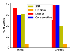
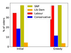
We tested our algorithm on $10$ neighboring constituencies out of the $650$ in the region of Scotland bordering Edinburgh, which represents a very diverse area in terms of voting preferences. Indeed, these neighboring constituencies voted very differently, each having a clear majority. For example, the distribution of votes in East Lothian was $36.3\%$ Labour, $29.8\%$ Conservative, $30.7$ Scottish National Party (SNP), and $3.1\%$ Liberal Democrats, while in Edinburgh East it was $34.6\%$ Labour, $18.5\%$ Conservative, $42.5\%$ SNP, and $4.2\%$ Liberal Democrats. We subsampled this dataset, working with a randomized sample of approximately $50,000$ people and we recorded the location of each constituencies (represented by its center), enforcing in Greedy Districting that voters can be incentivized to move or to vote only in their closest two constituencies.

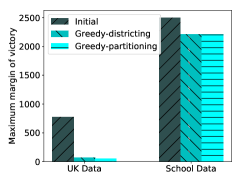
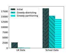
Figure 1(a) shows that both Greedy Districting and Greedy Partitioning are able to reduce the maximum margin of victory of this dataset by approximately $91-92\%$ percent, from $776$ to $67$ and $55$, respectively. Figure 1(c) shows the effect greedy had on minimizing the overall margin of victory, showing an even larger decrease by almost $95\%$, from $2652$ to $148$ and $135$, respectively. Since Greedy Districting represents the more realistic application, we show in Figure 2 its effect on the voters’ distribution in East Lothian and Edinburgh East, showing that it created a stronger opposition for the leading parties (for Labour in East Lothian and for SNP in Edinburgh East).

(a) East Lothian

(b) Edinburgh East

Figure 2: Voters’ distribution in UK constituencies before and after applying Greedy Districting.

(a) Dove Academy

(b) Universal Academy

(c) Cesar Chavez Academy

Figure 3: Racial distribution of students in selected schools before and after applying Greedy Districting.

US Public School Districting:

Neighborhood racial segregation is still widespread in many places in US, trickling down to segregation in schools (?; ?). One of the main consequences of that is white-majority schools receiving substantially more funding than schools with mostly students of color (?). In this paper, we attempt to show that our algorithms can be used to increase racial diversity (and lower segregation) in schools, if accompanied by government policies that facilitate movement of students between schools (?).

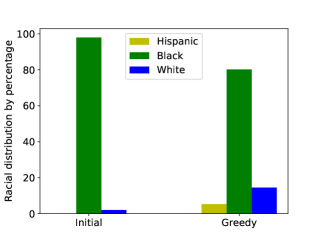
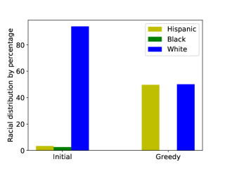
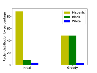
We collected school data from the National Center for Education Statistics (NCES: nces.ed.gov/ccd) about public schools in Detroit, MI, which is still one of the cities with highest rates of segregation and most economic and social struggles encountered by minorities (?; ?). We gathered data from $61$ schools in Detroit, each containing between $40$ and $5000$ students, summing up to $41,834$ students and their reported race. We modeled this data in the form of an election, where the $voters$ are the students and the $alternatives$ are their reported race (NCES data has $7$ reported races: Asian, Native American, Hispanic, Black, White, Hawaiian, and Mixed-race). Given each student’s race, we modeled this ‘election’ as a plurality voting scenario, where each student only ‘votes’ for their reported race. Furthermore, we recorded the location of each school, enforcing in Greedy Districting that students can only go to their closest $5$ schools.

Figure 1(a) shows that both Greedy Districting and Greedy Partitioning decrease the total margin of victory by $11-12\%$ on average, from $2,501$ to $2,213$ and $2,311$, respectively. Again, Figure 1(c) shows the overall decrease in margin of victory by the greedy algorithms, showing a larger decrease of $18-24\%$, from $18,870$ to $15,360$ and $14,376$, respectively. As Greedy Districting represents the more realistic scenario, we present in Figure 3 its effect on the racial distribution of students in a selection of three schools. we observe that schools containing students from one predominant racial group become more equilibrated: Dove Academy goes from having $98\%$ Black students and $2\%$ White to having $80\%$ Black, $14.5\%$ White, and $5.5\%$ Hispanic students, Universal Academy goes from having $95\%$ White students, $3.5\%$ Hispanic, and $2.5\%$ Black to having $50.15\%$ White and $49.7\%$ Hispanic, while Cesar Chavez Academy goes from having $88\%$ Hispanic students, $8\%$ Black, and $3\%$ White to having $48\%$ Hispanic, $48\%$ Black, and $3\%$ White students. Given the discrepancy between White-majority schools with other schools, we hope that such demographic changes can help in equalizing funding for all students.

Of course, since minimizing margin of victory only considers the most predominant two races, we may need to enforce an additional diversity constraint to preserve a minimum fraction of students from other races in a school (e.g., the $2.5\%$ Black students in Universal Academy may need to stay). We leave exploring this direction for future work.

Graph Simulations:

To further understand the relationship between margin of victory and population structure, we simulated a set of graphs based on the Erdos-Renyi (ER) graph model, varying the level of connectivity between people with similar political leanings. Unable to vary such a parameter in the real data, we turn to classical graph models to do so. Following the methodology in (?), we used the line model to simulate $voters$, $alternatives$, and $voters^{\prime}$ political affiliation. We then created $50$ instances of the ER graph model, where each node represents a $voter$ and the edges are formed according to the model with an added homophily factor based on the distance between nodes (as simulated by the line model). For every node, we generated the list of preferences over the candidates according to the distance between the voter and the candidates. The inputs to each such graph are the number of voters N (100), the number of candidates C (5), the number of districts K (5), and a homophily parameter.

Such models capture the network and clustering effects exhibited by voter districts in real world (?; ?; ?). We then test all three greedy algorithms in minimizing the maximum margin of victory by re-districting the population in these graphs. We further add a baseline algorithm that computes the optimal partition of voters into districts given a network, the districts’ size constraints, and mobility of voters. While Greedy Partitioning and Greedy Districting come as natural formulations, we argue the need for Greedy Connected Districting as well, since re-districting cannot be done arbitrarily and will be more effective if the population remain connected. Thus, in our simulations, the graph models aim to mimic the natural connections individuals make.

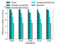
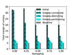
We simulated the greedy algorithm for each graph instance, averaging over $10$ iterations the minimal maximum margin of victory that it can reach and compared that to the baseline value. Figure 1(b) shows the effect of these algorithms in improving the maximum margin of victory aggregated for all graph instances, varying the homophily factor and allowing districts to change up to $20\%$ in size. We observe that no matter how homophilic the initial graph is, greedy is able to successfully reduce the margin of victory for all three algorithms: Greedy Partitioning performs the best as it contains no constraints on mobility of voters, being evaluated close to the baseline value and reducing maximum margin of victory from $10$ to $6-7$ on average, Greedy Districting performs second-best, reducing it from $10$ to $8$ on average, while Greedy Connected Districting reduces it from $10$ to $9$ on average, performing worse than the other two due to a tighter connectivity constraint. Figure 1(d) shows the overall decrease in margin of victory, where the effect is more significant: Greedy Partitioning and Greedy Districting achieve a result close to the baseline, while Greedy Connected Districting performs slightly worse, reducing the total margin of victory of $46\%$ on average. The results are qualitatively similar for varying the district size constraints, which we omit due to lack of space.

Conclusion and Future Directions

In this paper, we tackled the problem of fairly dividing people into groups by conceptualizing the problem in a voting scenario. By modeling the preferences of people over different candidates, we set the goal to minimize the maximum margin of victory in any group. In doing so, we provide a rigorous framework to reason about the complexity of the problem, showing that dividing people with constraints on their neighborhood or their connections is NP-complete in the most general case, and admit polynomial time algorithms for particular cases.

Furthermore, we develop and evaluate fast greedy heuristics to minimize the maximum margin of victory in practical scenarios. Indeed, our results show significant improvement of the margin of victory in the case of elections and school choice, as well as in synthetic experiments. In the case of elections, minimizing margin of victory leads to better representation of opposing parties in electoral districts, where we notice that the opposing parties in the UK can gain more power through re-districting. In the case of school choice, we model students demographic information as an election, where each student ’votes’ (or prefers) their own demographic attribute, and show that our greedy algorithms are able to provide more diversity in highly segregated schools. While government policies are ultimately crucial in reducing segregation, we hope that this quantitative analysis can motivate them and show their potential efficacy.

Multiple directions remain open for future work. We plan to (i) include an analysis of the social connections in real datasets that may further constrain people’s mobility, and (ii) extend synthetic experiments to other graph models as well. Finally, it would be interesting to (iii) measure the effect of minimizing the margin of victory on different gerrymandering metrics, and (iv) investigate whether lowering racial segregation would lead more equitable distribution of revenues to public schools.

References

- [Adamic and Glance 2005] Adamic, L. A., and Glance, N. 2005. The political blogosphere and the 2004 us election: divided they blog. In Proceedings of the 3rd international workshop on Link discovery, 36–43. ACM.
- [Bachrach et al. 2016] Bachrach, Y.; Lev, O.; Lewenberg, Y.; and Zick, Y. 2016. Misrepresentation in district voting. In IJCAI, 81–87.
- [Barbara and Garcia-Molina 1987] Barbara, D., and Garcia-Molina, H. 1987. The reliability of voting mechanisms. IEEE Transactions on Computers (10):1197–1208.
- [Barberà et al. 1991] Barberà, S.; Sonnenschein, H.; Zhou, L.; et al. 1991. Voting by committees. Econometrica 59(3):595–609.
- [Berman, Karpinski, and Scott 2003] Berman, P.; Karpinski, M.; and Scott, A. D. 2003. Approximation hardness and satisfiability of bounded occurrence instances of SAT. Electronic Colloquium on Computational Complexity (ECCC) 10(022).
- [Blom, Stuckey, and Teague 2018] Blom, M.; Stuckey, P. J.; and Teague, V. J. 2018. Computing the margin of victory in preferential parliamentary elections. In International Joint Conference on Electronic Voting, 1–16. Springer.
- [Borodin et al. 2018] Borodin, A.; Lev, O.; Shah, N.; and Strangway, T. 2018. Big city vs. the great outdoors: Voter distribution and how it affects gerrymandering. In IJCAI, 98–104.
- [Butler 1992] Butler, D. 1992. The redrawing of parliamentary boundaries in britain. British Elections and Parties Yearbook 2(1):5–12.
- [Chakraborty et al. 2019] Chakraborty, A.; Mota, N.; Biega, A. J.; Mohammadi, N.; Gummadi, K. P.; and Heidari, H. 2019. Nudging toward equitable online donations: A case study of educational charity.
- [Chang 2018] Chang, A. 2018. We can draw school zones to make classrooms less segregated. this is how well your district does.
- [Cohen-Zemach, Lewenberg, and Rosenschein 2018] Cohen-Zemach, A.; Lewenberg, Y.; and Rosenschein, J. S. 2018. Gerrymandering over graphs. In Proceedings of the 17th International Conference on Autonomous Agents and MultiAgent Systems, 274–282. International Foundation for Autonomous Agents and Multiagent Systems.
- [Conover et al. 2011] Conover, M. D.; Ratkiewicz, J.; Francisco, M.; Gonçalves, B.; Menczer, F.; and Flammini, A. 2011. Political polarization on twitter. In Fifth international AAAI conference on weblogs and social media.
- [Corsi-Bunker 2015] Corsi-Bunker, A. 2015. Guide to the education system in the united states. University of Minnesota 23.
- [Dey and Narahari 2015] Dey, P., and Narahari, Y. 2015. Estimating the margin of victory of an election using sampling. In Twenty-Fourth International Joint Conference on Artificial Intelligence.
- [Douglas N. Harris 2015] Douglas N. Harris, M. F. L. 2015. The identification of schooling preferences: methods and evidence from post-katrina new orleans.
- [EdBuild 2019] EdBuild. 2019. Non-white school districts get $23 billion less than white districts, despite serving the same number of students.
- [Erdélyi, Hemaspaandra, and Hemaspaandra 2015] Erdélyi, G.; Hemaspaandra, E.; and Hemaspaandra, L. A. 2015. More natural models of electoral control by partition. In International Conference on Algorithmic DecisionTheory, 396–413. Springer.
- [Feix et al. 2008] Feix, M. R.; Lepelley, D.; Merlin, V.; Rouet, J.-L.; and Vidu, L. 2008. Majority efficient representation of the citizens in a federal union. Manuscript, Université de la Réunion, Université de Caen, and Université d’Orléans.
- [Felsenthal and Miller 2015] Felsenthal, D. S., and Miller, N. R. 2015. What to do about election inversions under proportional representation? Representation 51(2):173–186.
- [Frankenberg 2019] Frankenberg, E. 2019. What school segregation looks like in the us today, in 4 charts.
- [Gelman, Katz, and Tuerlinckx 2002] Gelman, A.; Katz, J. N.; and Tuerlinckx, F. 2002. The mathematics and statistics of voting power. Statistical Science 420–435.
- [Institute 2018] Institute, U. 2018. Segregated neighborhoods, segregated schools?
- [Issacharoff 2002] Issacharoff, S. 2002. Gerrymandering and political cartels. Harvard Law Review 116.
- [Ito et al. 2019] Ito, T.; Kamiyama, N.; Kobayashi, Y.; and Okamoto, Y. 2019. Algorithms for gerrymandering over graphs. In Proceedings of the 18th International Conference on Autonomous Agents and MultiAgent Systems, 1413–1421. International Foundation for Autonomous Agents and Multiagent Systems.
- [Johnston, Rossiter, and Pattie 2006] Johnston, R.; Rossiter, D.; and Pattie, C. 2006. Disproportionality and bias in the results of the 2005 general election in great britain: evaluating the electoral system’s impact. Journal of Elections, Public Opinion and Parties 16(1):37–54.
- [Keegan 2016] Keegan, J. 2016. Blue feed, red feed. The Wall Street Journal 18.
- [Kent and Thomas C. Frohlich 2015] Kent, A., and Thomas C. Frohlich, H. P. 2015. The 9 most segregated cities in america.
- [Lewenberg, Lev, and Rosenschein 2017] Lewenberg, Y.; Lev, O.; and Rosenschein, J. S. 2017. Divide and conquer: Using geographic manipulation to win district-based elections. In AAMAS, 624–632.
- [Lublin 1999] Lublin, D. 1999. The paradox of representation: Racial gerrymandering and minority interests in Congress. Princeton University Press.
- [Montgomery III 1970] Montgomery III, J. 1970. Swann v. charlotte-mecklenburg board of education: Roadblocks to the implementation of brown. Wm. & Mary L. Rev. 12:838.
- [Richards 2014] Richards, M. P. 2014. The gerrymandering of school attendance zones and the segregation of public schools: A geospatial analysis. American Educational Research Journal 51(6):1119–1157.
- [van ’t Hof, Paulusma, and Woeginger 2009] van ’t Hof, P.; Paulusma, D.; and Woeginger, G. J. 2009. Partitioning graphs into connected parts. Theor. Comput. Sci. 410(47-49):4834–4843.
- [Xia 2012] Xia, L. 2012. Computing the margin of victory for various voting rules. In Proceedings of the 13th ACM Conference on Electronic Commerce, 982–999. ACM.