Modular Meta-Learning with Shrinkage

Abstract

Many real-world problems, including multi-speaker text-to-speech synthesis, can greatly benefit from the ability to meta-learn large models with only a few task-specific components. Updating only these task-specific modules then allows the model to be adapted to low-data tasks for as many steps as necessary without risking overfitting. Unfortunately, existing meta-learning methods either do not scale to long adaptation or else rely on handcrafted task-specific architectures. Here, we propose a meta-learning approach that obviates the need for this often sub-optimal hand-selection. In particular, we develop general techniques based on Bayesian shrinkage to automatically discover and learn both task-specific and general reusable modules. Empirically, we demonstrate that our method discovers a small set of meaningful task-specific modules and outperforms existing meta-learning approaches in domains like few-shot text-to-speech that have little task data and long adaptation horizons. We also show that existing meta-learning methods including MAML, iMAML, and Reptile emerge as special cases of our method.

1 Introduction

The goal of meta-learning is to extract shared knowledge from a large set of training tasks to solve held-out tasks more efficiently. One avenue for achieving this is to learn task-agnostic modules and reuse or repurpose these for new tasks. Reusing or repurposing modules can reduce overfitting in low-data regimes, improve interpretability, and facilitate the deployment of large multi-task models on limited-resource devices as parameter sharing allows for significant savings in memory. It can also enable batch evaluation of reused modules across tasks, which can speed up inference time on GPUs.

These considerations are important in domains like few-shot text-to-speech synthesis (TTS), characterized by large speaker-adaptable models, limited training data for speaker adaptation, and long adaptation horizons [1]. Adapting the model to a new task for more optimization steps generally improves the model capacity without increasing the number of parameters. However, many meta-learning methods are designed for quick adaptation, and hence are inapplicable in this few data and long adaptation regime. For those that are applicable [2, 3, 4, 5], adapting the full model to few data can then fail because of overfitting. To overcome this, modern TTS models combine shared core modules with handcrafted, adaptable, speaker-specific modules [6, 1, 7, 8]. This hard coding strategy is often suboptimal. As data increases, these hard-coded modules quickly become a bottleneck for further improvement, even in a few-shot regime. For this reason, we would like to automatically learn the smallest set of modules needed to adapt to a new speaker and then adapt these for as long as needed.

Automatically learning reusable and broadly applicable modular mechanisms is an open challenge in causality, transfer learning, and domain adaptation [9, 10, 11, 12]. In meta-learning, most existing gradient-based algorithms, such as MAML [13], do not encourage meta-training to develop reusable and general modules, and either ignore reusability or manually choose the modules to fix [14, 15, 5, 16, 17, 18]. Some methods implicitly learn a simple form of modularity for some datasets  [17, 19] but it is limited.

In this paper, we introduce a novel approach for automatically finding reusable modules. Our approach employs a principled hierarchical Bayesian model that exploits a statistical property known as shrinkage, meaning that low-evidence estimates tend towards their prior mean; e.g., see Gelman et al. [20]. This is accomplished by first partitioning any neural network into arbitrary groups of parameters, which we refer to as modules. We assign a Gaussian prior to each module with a scalar variance. When the variance parameter shrinks to zero for a specific module, as it does if the data does not require the module parameters to deviate from the prior mean, then all of the module’s parameters become tied to the prior mean during task adaptation. This results in a set of automatically learned modules that can be reused at deployment time and a sparse set of remaining modules that are adapted subject to the estimated prior.

Estimating the prior parameters in our model corresponds to meta-learning, and we present two principled methods for this based on maximizing the predictive log-likelihood. Importantly, both methods allow many adaptation steps. By considering non-modular variants of our model, we show that MAML [13], Reptile [2], and iMAML [3] emerge as special cases. We compare our proposed shrinkage-based methods with their non-modular baselines on multiple low-data, long-adaptation domains, including a challenging variant of Omniglot and TTS. Our modular, shrinkage-based methods exhibit higher predictive power in low-data regimes without sacrificing performance when more data is available. Further, the discovered modular structures corroborate common knowledge about network structure in computer vision and provide new insights about WaveNet [21] layers in TTS.

In summary, we introduce a hierarchical Bayesian model for modular meta-learning along with two parameter-estimation methods, which we show generalize existing meta-learning algorithms. We then demonstrate that our approach enables identification of a small set of meaningful task-specific modules. Finally, we show that our method prevents overfitting and improves predictive performance on problems that require many adaptation steps given only small amounts of data.

1.1 Related Work

Multiple Bayesian meta-learning approaches have been proposed to either provide model uncertainty in few-shot learning [22, 23, 24, 25] or to provide a probabilistic interpretation and extend existing non-Bayesian works [26, 27, 28]. However, to the best of our knowledge, none of these account for modular structure in their formulation. While we use point estimates of variables for computational reasons, more sophisticated inference methods from these works can also be used within our framework.

Modular meta-learning approaches based on MAML-style backpropagation through short task adaptation horizons have also been proposed. The most relevant of these, Alet et al. [29], proposes to learn a modular network architecture, whereas our work identifies the adaptability of each module. In other work, Zintgraf et al. [16] hand-designs the task-specific and shared parameters, and the M-Net in Lee and Choi [14] provides an alternative method for learning adaptable modules by sampling binary mask variables. In all of the above, however, backpropagating through task adaptation is computationally prohibitive when applied to problems that require longer adaptation horizons. While it is worth investigating how to extend these works to this setting, we leave this for future work.

Many other meta-learning works [14, 15, 5, 30, 31, 32] learn the learning rate (or a preconditioning matrix) which can have a similar modular regularization effect as our approach if applied modularly with fixed adaptation steps. However, these approaches and ours pursue fundamentally different and orthogonal goals. Learning the learning rate aims at fast optimization by fitting to local curvature, without changing the task loss or associated stationary point. In contrast, our method learns to control how far each module will move from its initialization by changing that stationary point. In problems requiring long task adaptation, these two approaches lead to different behaviors, as we demonstrate in Appendix C. Further, most of these works also rely on backpropagating through gradients, which does not scale well to the long adaptation horizons considered in this work. Overall, generalizing beyond the training horizon is challenging for “learning-to-optimize” approaches  [33, 34]. While WarpGrad [5] does allow long adaptation horizons, it is not straightforward to apply its use of a functional mapping from inputs to a preconditioning matrix for module discovery and we leave this for future work.

Finally, L2 regularization is also used for task adaptation in continual learning [35, 36] and meta-learning [37, 38, 39, 3]. However, in these works, the regularization scale(s) are either treated as hyper-parameters or adapted per dimension with a different criterion from our approach. It is not clear how to learn the regularization scale at a module level in these works.

2 Gradient-based Meta-Learning

We begin with a general overview of gradient-based meta-learning, as this is one of the most common approaches to meta-learning. In this regime, we assume that there are many tasks, indexed by $t$, and that each of these tasks has few data. That is, each task is associated with a finite dataset $\mathcal{D}_{t}=\{\mathbf{x}_{t,n}\}$ of size $N_{t}$, which can be partitioned into training and validation sets, $\mathcal{D}_{t}^{\text{train}}$ and $\mathcal{D}_{t}^{\text{val}}$ respectively.  To solve a task, gradient-based meta-learning adapts task-specific parameters $\boldsymbol{\theta}_{t}\in{}^{D}$ by minimizing a loss function $\ell(\mathcal{D}_{t};\boldsymbol{\theta}_{t})$ using a local optimizer. Adaptation is made more efficient by sharing a set of meta parameters $\boldsymbol{\phi}\in{}^{D}$ between tasks, which are typically used to initialize the task parameters.

Algorithm 1 summarizes a typical stochastic meta-training procedure, which includes MAML [13], implicit MAML (iMAML) [3], and Reptile [2]. Here, TaskAdapt executes one step of optimization of the task parameters. The meta-update $\Delta_{t}$ specifies the contribution of task $t$ to the meta parameters. At test time, multiple steps of TaskAdapt are run on each new test task.

Input: Batch size $B$, steps $L$, and learning rate $\alpha$

Initialize $\boldsymbol{\phi}$

while not done do

       $\{t_{1},\dots,t_{B}\}\leftarrow$ sample mini-batch of tasks

       for each task $t$ in $\{t_{1},\dots,t_{B}\}$ do

             Initialize $\boldsymbol{\theta}_{t}\leftarrow\boldsymbol{\phi}$

             for step $l=1\dots L$ do

                   $\boldsymbol{\theta}_{t}\leftarrow\textsc{TaskAdapt}(\mathcal{D}_{t},\boldsymbol{\phi},\boldsymbol{\theta}_{t})$

             end for

            

       end for

      

       // Meta update

       $\boldsymbol{\phi}\leftarrow\boldsymbol{\phi}-\alpha\cdot\frac{1}{B}\sum_{t}\Delta_{t}(\mathcal{D}_{t},\boldsymbol{\phi},\boldsymbol{\theta}_{t})$

      

end while

Algorithm 1 Meta-learning pseudocode.

Figure 1: (Left) Structure of a typical meta-learning algorithm. (Right) Bayesian shrinkage graphical model. The shared meta parameters $\boldsymbol{\phi}$ serve as the initialization of the neural network parameters for each task $\boldsymbol{\theta}_{t}$. The $\boldsymbol{\sigma}$ are shrinkage parameters. By learning these, the model automatically decides which subsets of parameters (i.e., modules) to fix for all tasks and which to adapt at test time.

MAML implements task adaptation by applying gradient descent to minimize the training loss $\ell_{t}^{\text{train}}(\boldsymbol{\theta}_{t})=\ell(\mathcal{D}^{\text{train}}_{t};\boldsymbol{\theta}_{t})$ with respect to the task parameters. It then updates the meta parameters by gradient descent on the validation loss $\ell_{t}^{\text{val}}(\boldsymbol{\theta}_{t})=\ell(\mathcal{D}^{\text{val}}_{t};\boldsymbol{\theta}_{t})$, resulting in the meta update $\Delta_{t}^{\text{MAML}}=\nabla_{\boldsymbol{\phi}}\,\ell_{t}^{\text{val}}(\boldsymbol{\theta}_{t}(\boldsymbol{\phi})).$ This approach treats the task parameters as a function of the meta parameters, and hence requires backpropagating through the entire $L$-step task adaptation process. When $L$ is large, as in TTS systems [1], this becomes computationally prohibitive.

Reptile and iMAML avoid this computational burden of MAML. Reptile instead optimizes $\boldsymbol{\theta}_{t}$ on the entire dataset $\mathcal{D}_{t}$, and moves $\boldsymbol{\phi}$ towards the adapted task parameters, yielding $\Delta_{t}^{\text{Reptile}}=\boldsymbol{\phi}-\boldsymbol{\theta}_{t}.$ Conversely, iMAML introduces an L2 regularizer $\frac{\lambda}{2}||\boldsymbol{\theta}_{t}-\boldsymbol{\phi}||^{2}$ and optimizes the task parameters on the regularized training loss. Provided that this task adaptation process converges to a stationary point, implicit differentiation enables the computation of the meta gradient based only on the final solution of the adaptation process, $\Delta_{t}^{\text{iMAML}}=\big{(}\mathbf{I}+\tfrac{1}{\lambda}\nabla^{2}_{\boldsymbol{\theta}_{t}}\ell_{t}^{\text{train}}(\boldsymbol{\theta}_{t})\big{)}^{-1}\nabla_{\boldsymbol{\theta}_{t}}\ell_{t}^{\text{val}}(\boldsymbol{\theta}_{t}).$ See Rajeswaran et al. [3] for details.

3 Modular Bayesian Meta-Learning

In standard meta-learning, the meta parameters $\boldsymbol{\phi}$ provide an initialization for the task parameters $\boldsymbol{\theta}$ at test time. That is, all the neural network parameters are treated equally, and hence they must all be updated at test time. This strategy is inefficient and prone to overfitting. To overcome it, researchers often split the network parameters into two groups, a group that varies across tasks and a group that is shared; see for example [1, 16]. This division is heuristic, so in this work we explore ways of automating it to achieve better results and to enable automatic discovery of task independent modules. More precisely, we assume that the network parameters can be partitioned into $M$ disjoint modules $\boldsymbol{\theta}_{t}=(\boldsymbol{\theta}_{t,1},\ldots,\boldsymbol{\theta}_{t,m},\ldots,\boldsymbol{\theta}_{t,M})$ where $\boldsymbol{\theta}_{t,m}$ are the parameters in module $m$ for task $t$. This view of modules is very general. Modules can correspond to layers, receptive fields, the encoder and decoder in an auto-encoder, the heads in a multi-task learning model, or any other grouping of interest.

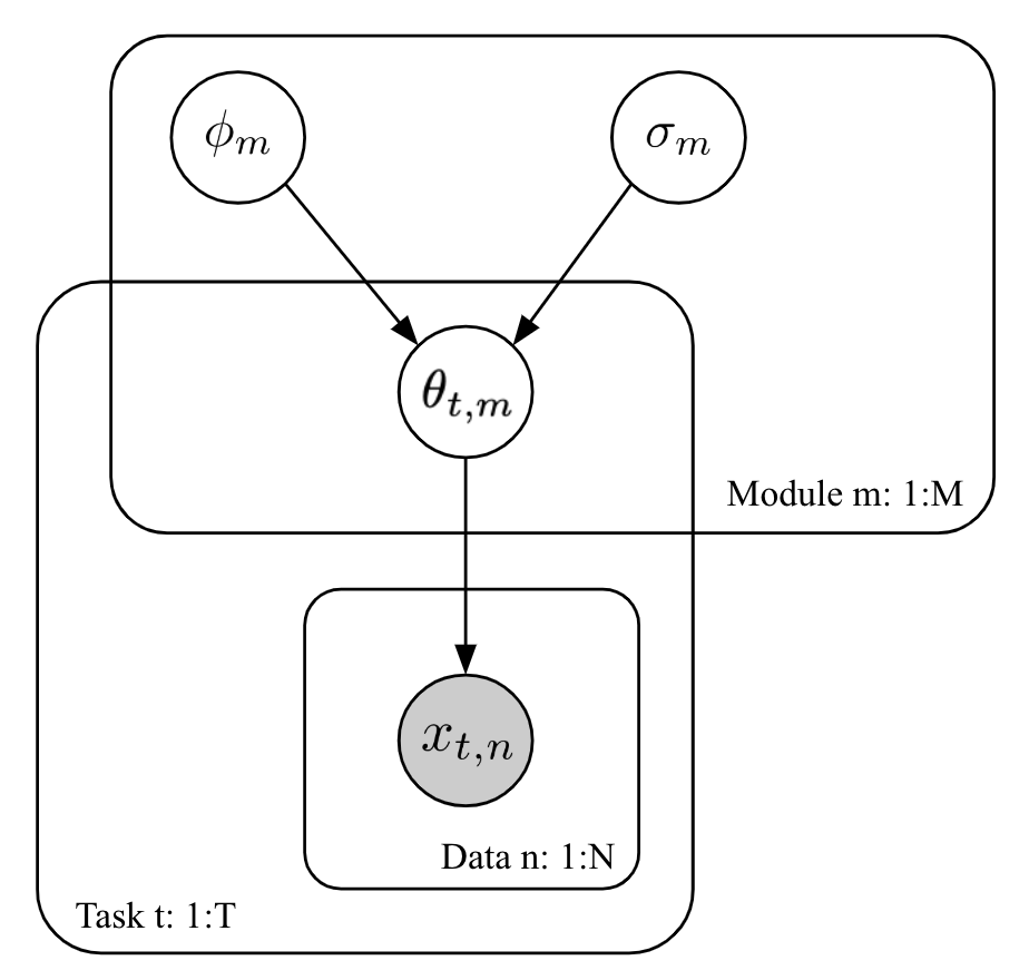
We adopt a hierarchical Bayesian model, shown in Figure 1, with a factored probability density:

$$p(\boldsymbol{\theta}_{1:T},\mathcal{D}|\boldsymbol{\sigma}^{2},\boldsymbol{\phi})=\prod_{t=1}^{T}\prod_{m=1}^{M}{\cal N}(\boldsymbol{\theta}_{t,m}|\boldsymbol{\phi}_{m},\sigma_{m}^{2}\mathbf{I})\prod_{t=1}^{T}p(\mathcal{D}_{t}|\boldsymbol{\theta}_{t}).$$ (1)

The $\boldsymbol{\theta}_{t,m}$ are conditionally independent and normally distributed $\boldsymbol{\theta}_{t,m}\sim{\cal N}(\boldsymbol{\theta}_{t,m}|\boldsymbol{\phi}_{m},\sigma_{m}^{2}\mathbf{I})$ with mean $\boldsymbol{\phi}_{m}$ and variance $\sigma_{m}^{2}$, where $\mathbf{I}$ is the identity matrix.

The $m$-th module scalar shrinkage parameter $\sigma_{m}^{2}$ measures the degree to which $\boldsymbol{\theta}_{t,m}$ can deviate from $\boldsymbol{\phi}_{m}$. More precisely, for values of $\sigma_{m}^{2}$ near zero, the difference between parameters $\boldsymbol{\theta}_{t,m}$ and mean $\boldsymbol{\phi}_{m}$ will be shrunk to zero and thus module $m$ will become task independent. Thus by learning the parameters $\boldsymbol{\sigma}^{2}$, we discover which modules are task independent. These independent modules can be reused at test time, reducing the computational burden of adaptation and likely improving generalization. Shrinkage is often used in automatic relevance determination for sparse feature selection [40].

We place uninformative priors on $\boldsymbol{\phi}_{m}$ and $\sigma_{m}$, and follow an empirical Bayes approach to learn their values from data. This formulation allows the model to automatically learn which modules to reuse—i.e. those modules for which $\sigma_{m}^{2}$ is near zero—and which to adapt at test time.

4 Meta-Learning as Parameter Estimation

By adopting the hierarchical Bayesian model from the previous section, the problem of meta-learning becomes one of estimating the parameters $\boldsymbol{\phi}$ and $\boldsymbol{\sigma}^{2}$. A standard solution to this problem is to maximize the marginal likelihood $p(\mathcal{D}|\boldsymbol{\phi},\boldsymbol{\sigma}^{2})=\int p(\mathcal{D}|\boldsymbol{\theta})p(\boldsymbol{\theta}|\boldsymbol{\phi},\boldsymbol{\sigma}^{2})\,\textrm{d}\boldsymbol{\theta}$. We can also assign a prior over $\boldsymbol{\phi}$. In both cases, the marginalizations are intractable, so we must seek scalable approximations.

It may be tempting to estimate the parameters by maximizing $p(\boldsymbol{\theta}_{1:T},\mathcal{D}|\boldsymbol{\sigma}^{2},\boldsymbol{\phi})$ w.r.t. $(\boldsymbol{\sigma}^{2},\boldsymbol{\phi},\boldsymbol{\theta}_{1:T})$, but the following lemma suggests that this naive approach leads to all task parameters being tied to the prior mean, i.e. no adaptation will occur (see Appendix A for a proof):

Lemma 1.

The function $f:(\boldsymbol{\sigma}^{2},\boldsymbol{\phi},\boldsymbol{\theta}_{1:T})\mapsto\log p(\boldsymbol{\theta}_{1:T},\mathcal{D}|\boldsymbol{\sigma}^{2},\boldsymbol{\phi})$ diverges to $+\infty$ as $\boldsymbol{\sigma}^{2}\rightarrow 0^{+}$ when $\boldsymbol{\theta}_{t,m}=\boldsymbol{\phi}_{m}$ for all $t\in\{1,...,T\},m\in\{1,...,M\}$.

The undesirable result of Lemma 1 is caused by the use of point estimate of $\boldsymbol{\theta}_{1:T}$ in maximum likelihood estimation of $\boldsymbol{\sigma}^{2}$ and $\boldsymbol{\phi}$. In the following two subsections, we propose two principled alternative approaches for parameter estimation based on maximizing the predictive likelihood over validation subsets.

4.1 Parameter estimation via the predictive likelihood

Our goal is to minimize the average negative predictive log-likelihood over $T$ validation tasks,

$$\ell_{\mathrm{PLL}}(\boldsymbol{\sigma}^{2},\boldsymbol{\phi}) =-\frac{1}{T}\sum_{t=1}^{T}\log p\left(\mathcal{D}_{t}^{\text{val}}|\mathcal{D}_{t}^{\text{train}},\boldsymbol{\sigma}^{2},\boldsymbol{\phi}\right)=\frac{1}{T}\sum_{t=1}^{T}\log\int p(\mathcal{D}_{t}^{\text{val}}|\boldsymbol{\theta}_{t})\,p(\boldsymbol{\theta}_{t}|\mathcal{D}_{t}^{\text{train}},\boldsymbol{\sigma}^{2},\boldsymbol{\phi})\,\textrm{d}\boldsymbol{\theta}_{t}.$$ (2)

To justify this goal, assume that the training and validation data is distributed i.i.d according to some distribution $\nu(\mathcal{D}_{t}^{\text{train}},\mathcal{D}_{t}^{\text{val}})$. Then, the law of large numbers implies that as $T\rightarrow\infty$,

$$\ell_{\mathrm{PLL}}(\boldsymbol{\sigma}^{2},\boldsymbol{\phi})\rightarrow\mathbb{E}_{\nu(\mathcal{D}_{t}^{\text{train}})}[\textrm{KL}(\nu(\mathcal{D}_{t}^{\text{val}}|\mathcal{D}_{t}^{\text{train}})||p\left(\mathcal{D}_{t}^{\text{val}}|\mathcal{D}_{t}^{\text{train}},\boldsymbol{\sigma}^{2},\boldsymbol{\phi}\right))]+\textrm{H}(\nu(\mathcal{D}_{t}^{\text{val}}|\mathcal{D}_{t}^{\text{train}})),$$ (3)

where KL denotes the Kullback-Leibler divergence and H the entropy. Thus minimizing $\ell_{\mathrm{PLL}}$ with respect to the meta parameters corresponds to selecting the predictive distribution $p\left(\mathcal{D}_{t}^{\text{val}}|\mathcal{D}_{t}^{\text{train}},\boldsymbol{\sigma}^{2},\boldsymbol{\phi}\right)$ that is closest (approximately) to the true predictive distribution $\nu(\mathcal{D}_{t}^{\text{val}}|\mathcal{D}_{t}^{\text{train}})$ on average. This criterion can be thought of as an approximation to a Bayesian cross-validation criterion [41].

Computing $\ell_{\mathrm{PLL}}$ is not feasible due to the intractable integral in equation (2). Instead we make use of a simple maximum a posteriori (MAP) approximation of the task parameters:

$$\hat{\boldsymbol{\theta}}_{t}(\boldsymbol{\sigma}^{2},\boldsymbol{\phi})=\operatorname*{argmin}\limits_{\boldsymbol{\theta}_{t}}\ell_{t}^{\text{train}}(\boldsymbol{\theta}_{t},\boldsymbol{\sigma}^{2},\boldsymbol{\phi}),~{}\text{where }\ell_{t}^{\text{train}}\coloneqq-\log p\left(\mathcal{D}_{t}^{\text{train}}|\boldsymbol{\theta}_{t}\right)-\log p\left(\boldsymbol{\theta}_{t}|\boldsymbol{\sigma}^{2},\boldsymbol{\phi}\right).$$ (4)

We note for clarity that $\ell_{t}^{\text{train}}$ corresponds to the negative log of equation (1) for a single task. Using these MAP estimates, we can approximate $\ell_{\mathrm{PLL}}(\boldsymbol{\sigma}^{2},\boldsymbol{\phi})$ as follows:

$$\hat{\ell}_{\mathrm{PLL}}(\boldsymbol{\sigma}^{2},\boldsymbol{\phi})=\frac{1}{T}\sum_{t=1}^{T}\ell_{t}^{\text{val}}(\hat{\boldsymbol{\theta}}_{t}(\boldsymbol{\sigma}^{2},\boldsymbol{\phi})),\;\;~{}\text{ where }\ell_{t}^{\text{val}}\coloneqq-\log p\big{(}\mathcal{D}_{t}^{\text{val}}|\hat{\boldsymbol{\theta}}_{t}\big{)}.$$ (5)

We use this loss to construct a meta-learning algorithm with the same structure as Algorithm 1. Individual task adaptation follows from equation (4) and meta updating from minimizing $\hat{\ell}_{\mathrm{PLL}}(\boldsymbol{\sigma}^{2},\boldsymbol{\phi})$ in equation (5) with an unbiased gradient estimator and a mini-batch of sampled tasks.

Minimizing equation (5) is a bi-level optimization problem that requires solving equation (4) implicitly. If optimizing $\ell_{t}^{\text{train}}$ requires only a small number of local optimization steps, we can compute the update for $\boldsymbol{\phi}$ and $\boldsymbol{\sigma}^{2}$ with back-propagation through $\hat{\boldsymbol{\theta}}_{t}$, yielding

$$\Delta_{t}^{\text{$\boldsymbol{\sigma}${}-MAML{}}}=\nabla_{\boldsymbol{\sigma}^{2},\boldsymbol{\phi}}\,\ell_{t}^{\text{val}}(\hat{\boldsymbol{\theta}}_{t}(\boldsymbol{\sigma}^{2},\boldsymbol{\phi})).$$ (6)

This update reduces to that of MAML if $\sigma_{m}^{2}\rightarrow\infty$ for all modules and is thus denoted as $\boldsymbol{\sigma}$-MAML.

We are however more interested in long adaptation horizons for which back-propagation through the adaptation becomes computationally expensive and numerically unstable. Instead, we apply the implicit function theorem on equation (4) to compute the gradient of $\hat{\boldsymbol{\theta}}_{t}$ with respect to $\boldsymbol{\sigma}^{2}$ and $\boldsymbol{\phi}$, giving

$$\Delta_{t}^{\text{$\boldsymbol{\sigma}${}-iMAML{}}}=-\nabla_{\boldsymbol{\theta}_{t}}\ell_{t}^{\text{val}}(\boldsymbol{\theta}_{t})\mathbf{H}_{\boldsymbol{\theta}_{t}\boldsymbol{\theta}_{t}}^{-1}\mathbf{H}_{\boldsymbol{\theta}_{t}\boldsymbol{\Phi}},$$ (7)

where $\boldsymbol{\Phi}=(\boldsymbol{\sigma}^{2},\boldsymbol{\phi})$ is the full vector of meta-parameters, $\mathbf{H}_{ab}=\nabla_{a,b}^{2}\ell_{t}^{\text{train}}$, and derivatives are evaluated at the stationary point $\boldsymbol{\theta}_{t}=\hat{\boldsymbol{\theta}}_{t}(\boldsymbol{\sigma}^{2},\boldsymbol{\phi})$. A detailed derivation is provided in Section B.1. Various approaches have been proposed to approximate the inverse Hessian [3, 42, 43, 44]. We use the conjugate gradient algorithm. We show in Section B.2 that the meta update for $\boldsymbol{\phi}$ is equivalent to that of iMAML when $\sigma_{m}^{2}$ is constant for all $m$, and thus refer to this more general method as $\boldsymbol{\sigma}$-iMAML.

In summary, our goal of maximizing the predictive likelihood of validation data conditioned on training data for our hierarchical Bayesian model results in modular generalizations of the MAML and iMAML approaches. In the following subsection, we will see that the same is also true for Reptile.

4.2 Estimating $\boldsymbol{\phi}$ via MAP approximation

If we instead let $\boldsymbol{\phi}$ be a random variable with prior distribution $p(\boldsymbol{\phi})$, then we can derive a different variant of the above algorithm. We return to the predictive log-likelihood introduced in the previous section but now integrate out the central parameter $\boldsymbol{\phi}$. Since $\boldsymbol{\phi}$ depends on all training data we will rewrite the average predictive likelihood in terms of the joint posterior over $(\boldsymbol{\theta}_{1:T},\boldsymbol{\phi})$, i.e.

$$\ell_{\mathrm{PLL}}(\boldsymbol{\sigma}^{2}) =-\frac{1}{T}\log p(\mathcal{D}_{1:T}^{\text{val}}|\mathcal{D}_{1:T}^{\text{train}},\boldsymbol{\sigma}^{2})=-\frac{1}{T}\log\int\Big{(}\prod_{t=1}^{T}p(\mathcal{D}_{t}^{\text{val}}|\boldsymbol{\theta}_{t})\Big{)}p(\boldsymbol{\theta}_{1:T},\boldsymbol{\phi}|\mathcal{D}_{1:T}^{\text{train}},\boldsymbol{\sigma}^{2})\textrm{d}\boldsymbol{\theta}_{1:T}\textrm{d}\boldsymbol{\phi}.$$ (8)

Again, to address the intractable integral we make use of a MAP approximation, except in this case we approximate both the task parameters and the central meta parameter as

$$(\hat{\boldsymbol{\theta}}_{1:T}(\boldsymbol{\sigma}^{2}),\hat{\boldsymbol{\phi}}(\boldsymbol{\sigma}^{2}))=\operatorname*{argmin}\limits_{\boldsymbol{\theta}_{1:T},\boldsymbol{\phi}}\,-\log p(\boldsymbol{\theta}_{1:T},\boldsymbol{\phi}|\mathcal{D}_{1:T}^{\text{train}},\boldsymbol{\sigma}^{2})=\operatorname*{argmin}\limits_{\boldsymbol{\theta}_{1:T},\boldsymbol{\phi}}\sum_{t=1}^{T}\ell_{t}^{\text{train}}(\boldsymbol{\theta}_{t},\boldsymbol{\sigma}^{2},\boldsymbol{\phi})-\log p(\boldsymbol{\phi}).$$ (9)

We assume a flat prior for $\boldsymbol{\phi}$ in this paper and thus drop the second term above. Note that when the number of training tasks $T$ is small, an informative prior would be preferred. We can then estimate the shrinkage parameter $\boldsymbol{\sigma}^{2}$ by plugging this approximation into Eq. 8. This method gives the same task adaptation update as the previous section but a meta update of the form

$$\Delta_{t,\boldsymbol{\phi}_{m}}^{\text{$\boldsymbol{\sigma}${}-Reptile{}}}=\frac{1}{\sigma_{m}^{2}}(\boldsymbol{\phi}_{m}-\hat{\boldsymbol{\theta}}_{m,t}),~{}~{}\Delta_{t,\boldsymbol{\sigma}^{2}}^{\text{$\boldsymbol{\sigma}${}-Reptile{}}}=-\nabla_{\boldsymbol{\theta}_{t}}\ell_{t}^{\text{val}}(\boldsymbol{\theta}_{t})\mathbf{H}_{\boldsymbol{\theta}_{t}\boldsymbol{\theta}_{t}}^{-1}\mathbf{H}_{\boldsymbol{\theta}_{t}\boldsymbol{\sigma}^{2}}\,,$$ (10)

where derivatives are evaluated at $\boldsymbol{\theta}_{t}=\hat{\boldsymbol{\theta}}_{t}(\boldsymbol{\sigma}^{2})$, and the gradient of $\hat{\boldsymbol{\phi}}$ w.r.t. $\boldsymbol{\sigma}^{2}$ is ignored. Due to lack of space, further justification and derivation of this approach is provided in Sections B.3 and B.4.

We can see that Reptile is a special case of this method when $\sigma_{m}^{2}\rightarrow\infty$ and we choose a learning rate proportional to $\sigma_{m}^{2}$ for $\boldsymbol{\phi}_{m}$. We thus refer to it as $\boldsymbol{\sigma}$-Reptile.

Table 1 compares our proposed algorithms with existing algorithms in the literature. Our three algorithms reduce to the algorithms on the left when $\sigma_{m}^{2}\rightarrow\infty$ or a constant scalar for all modules. Another variant of MAML for long adaptation, first-order MAML, can be recovered as a special case of iMAML when using one step of conjugate gradient descent to compute the inverse Hessian [3].

		Fixed $\boldsymbol{\sigma}^{2}$	Learned $\boldsymbol{\sigma}^{2}$	Allows long adaptation?
$\hat{\boldsymbol{\phi}}_{\mathrm{joint}}$		Reptile	$\boldsymbol{\sigma}$-Reptile	✓
$\hat{\boldsymbol{\phi}}_{\mathrm{PLL}}$	Back-prop.	MAML	$\boldsymbol{\sigma}$-MAML	$\times$
	Implicit grad.	iMAML	$\boldsymbol{\sigma}$-iMAML	✓

Table 1: The above algorithms result from different approximations to the predictive likelihood.

4.3 Task-Specific Module Selection

When the parameters $\boldsymbol{\phi}$ and $\boldsymbol{\sigma}^{2}$ are estimated accurately, the values of $\sigma_{m}^{2}$ for task-independent modules shrink towards zero. The remaining modules with non-zero $\sigma_{m}^{2}$ are considered task-specific [40]. In practice, however, the estimated value of $\sigma_{m}^{2}$ will never be exactly zero due to the use of stochastic optimization and the approximation in estimating the meta gradients. We therefore apply a weak regularization on $\boldsymbol{\sigma}^{2}$ to encourage its components to be small unless nonzero values are supported by evidence from the task data (see Appendix D for details).

While the learned $\sigma_{m}^{2}$ values are still non-zero, in most of our experiments below, the estimated value $\sigma_{m}^{2}$ for task-independent modules is either numerically indistinguishable from $0$ or at least two orders of magnitude smaller than the value for the task-specific modules. This reduces the gap between meta-training, where all modules have non-zero $\sigma_{m}^{2}$, and meta-testing, where a sparse set of modules are selected for adaptation. The exception to this is the text-to-speech experiment where we find the gap of $\sigma_{m}^{2}$ between modules to not be as large as in the image experiments. Thus, we instead rank the modules by the value of $\sigma_{m}^{2}$ and select the top-ranked modules as task-specific.

Ranking and selecting task-specific modules using the estimated value of $\sigma_{m}^{2}$ allows us to trade off between module sparsity and model capacity in practice, and achieves robustness against overfitting. It remains unclear in theory, however, if the task sensitivity of a module is always positively correlated with $\sigma_{m}^{2}$ especially when the size of modules varies widely. This is an interesting question that we leave for future investigation.

5 Experimental Evaluation

We evaluate our shrinkage-based methods on challenging meta-learning domains that have small amounts of data and require long adaptation horizons, such as few-shot text-to-speech voice synthesis. The aim of our evaluation is to answer the following three questions: (1) Does shrinkage enable automatic discovery of a small set of task-specific modules? (2) Can we adapt only the task-specific modules without sacrificing performance? (3) Does incorporating a shrinkage prior improve performance and robustness to overfitting in problems with little data and long adaptation horizons?

5.1 Experiment setup

Our focus is on long adaptation, low data regimes. To this end, we compare iMAML and Reptile to their corresponding shrinkage variants, $\boldsymbol{\sigma}$-iMAML and $\boldsymbol{\sigma}$-Reptile. For task adaptation with the shrinkage variants, we use proximal gradient descent [45] for the image experiments, and introduce a proximal variant of Adam [46] (pseudocode in Algorithm 3) for the text-to-speech (TTS) experiments. The proximal methods provide robustness to changes in the prior strength $\boldsymbol{\sigma}^{2}$ over time. We provide further algorithmic details in Appendix D. We evaluate on the following domains.

Few-shot image classification. We use the augmented Omniglot protocol of Flennerhag et al. [4], which necessitates long-horizon adaptation. For each alphabet, $20$ characters are sampled to define a $20$-class classification problem. The domain is challenging because both train and test images are randomly augmented. Following Flennerhag et al. [4], we use a 4-layer convnet and perform $100$ steps of task adaptation. We consider two regimes: (Large-data regime) We use $30$ training alphabets ($T=30$), $15$ training images ($K=15$), and $5$ validation images per class. Each image is randomly re-scaled, translated, and rotated. (Small-data regime) To study the effect of overfitting, we vary $T\in\{5,10,15,20\}$ and $K\in\{1,3,5,10,15\}$, and augment only by scaling and translating.

Text-to-speech voice synthesis. Training a neural TTS model from scratch typically requires tens of hours of speech data. In the few-shot learning setting [6, 1, 7, 8], the goal is to adapt a trained model to a new speaker based on only a few minutes of data. Earlier work unsuccessfully applied fast-adaptation methods such as MAML to synthesizing utterances [1]. Instead, their state-of-the-art method first pretrains a multi-speaker model comprised of a shared core network and a speaker embedding module and then finetunes either the entire model or the embedding only. We remove the manually-designed speaker embedding layers and perform task adaptation and meta-updates on only the core network.

The core network is a WaveNet vocoder model [21] with $30$ residual causal dilated convolutional blocks as the backbone, consisting of roughly 3M parameters. For computational reasons, we use only one quarter of the channels of the standard network. As a result, sample quality does not reach production level but we expect the comparative results to apply to the full network. We meta-train with tasks of $100$ training utterances (about $8$ minutes) using 100 task adaptation steps, then evaluate on held-out speakers with either $100$ or $50$ (about $4$ minutes) utterances and up to $10,000$ adaptation steps. For more details see Section E.2.

Short adaptation. While our focus is on long adaptation, we conduct experiments on short-adaptation datasets (sinusoid regression, standard Omniglot, and miniImageNet) for completeness in Appendix E.

5.2 Module discovery

To determine whether shrinkage discovers task-specific modules, we examine the learned prior strengths of each module and then adapt individual (or a subset of the) modules to assess the effect on performance due to adapting the chosen modules. In these experiments, we treat each layer as a module but other choices of modules are straightforward.

(a) $\boldsymbol{\sigma}^{2}$ for $\boldsymbol{\sigma}$-iMAML.

(b) $\boldsymbol{\sigma}^{2}$ for $\boldsymbol{\sigma}$-Reptile.

(c) $\boldsymbol{\sigma}$-iMAML accuracy.

(d) $\boldsymbol{\sigma}$-Reptile accuracy.

Figure 2: Module discovery with $\boldsymbol{\sigma}$-iMAML and $\boldsymbol{\sigma}$-Reptile for large-data augmented Omniglot. (a,b) The learned $\boldsymbol{\sigma}^{2}$ for each module (y-axis is log scale). (c,d) Test accuracy when only that layer is adapted versus when all layers are adapted using the learned $\boldsymbol{\sigma}^{2}$.

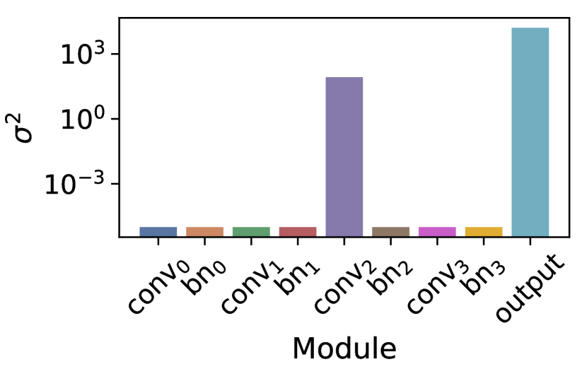
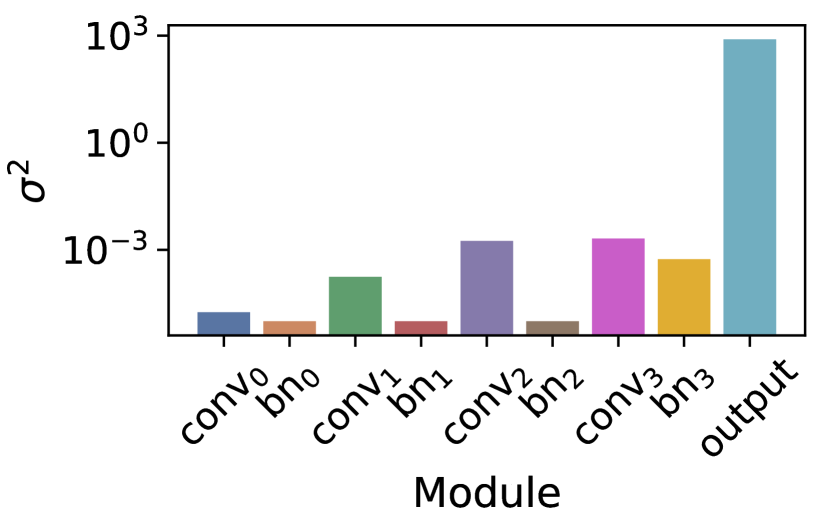
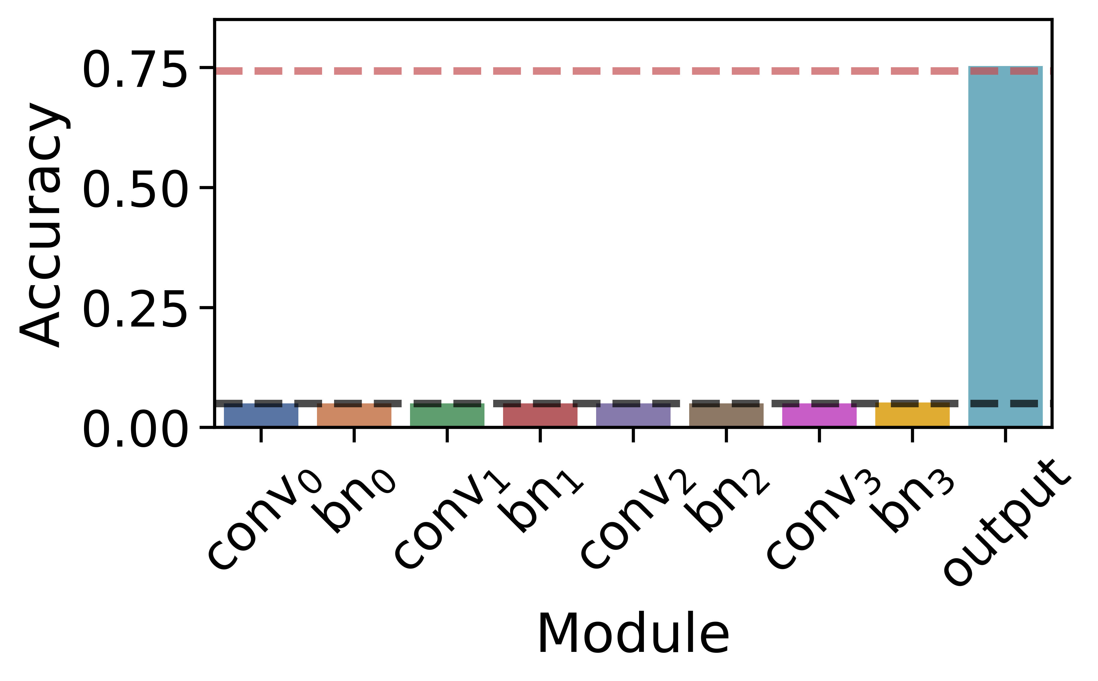
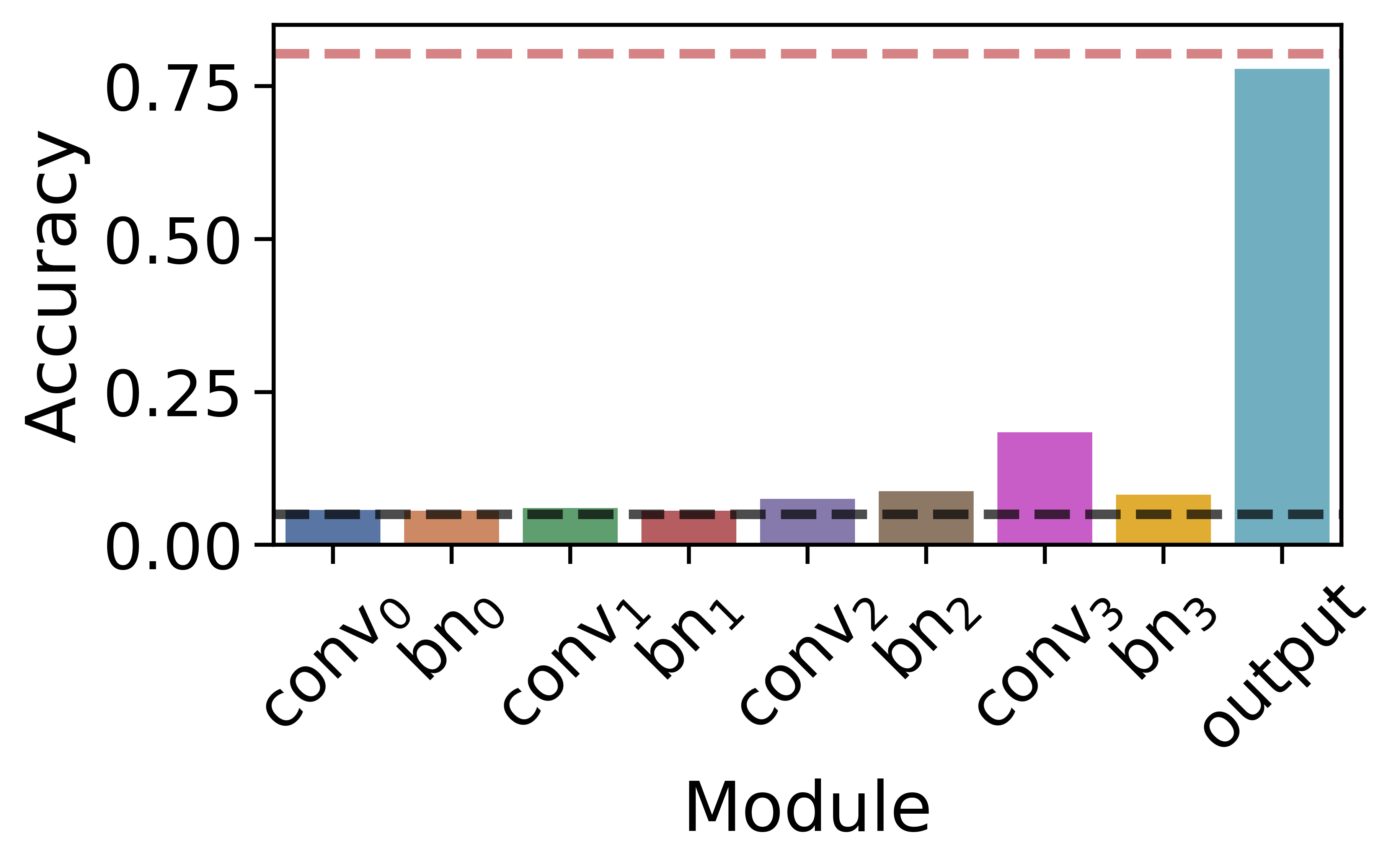
Image classification. Fig. 2 shows our module discovery results on large-data augmented Omniglot for $\boldsymbol{\sigma}$-iMAML and $\boldsymbol{\sigma}$-Reptile using the standard network (4 conv layers, 4 batch-norm layers, and a linear output layer). In each case, the learned $\boldsymbol{\sigma}^{2}$ (Fig. 2(a,b)) of the output layer is considerably larger than the others. Fig. 2(c,d) show that the model achieves high accuracy when adapting only this shrinkage-identified module, giving comparable performance to that achieved by adapting all layers according to $\boldsymbol{\sigma}^{2}$. This corroborates the conventional belief that the output layers of image classification networks are more task-specific while the input layers are more general, and bolsters other meta-learning studies [17, 25] that propose to adapt only the output layer.

However, the full story is not so clear cut. Our module discovery results (Appendix E) on standard few-shot short-adaptation image classification show that in those domains adapting the penultimate layer is best, which matches an observation in Arnold et al. [19]. Further, on sinusoid regression, adapting the first layer performed best. Thus, there is no single best modular structure across domains.

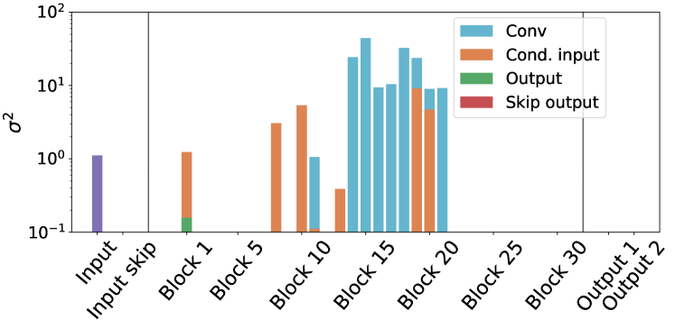
Text-to-speech. Fig. 3 shows the learned $\sigma^{2}$ for each layer of our TTS WaveNet model, which consists of 4 layers per residual block and 123 layers in total (Section E.2 shows the full architecture). Most $\sigma^{2}$ values are too small to be visible. The dilated conv layers between blocks 10 and 21 have the largest $\sigma^{2}$ values and thus require the most adaptability, suggesting that these blocks model the most speaker-specific features. These layers have a receptive field of $43$–$85$ ms, which matches our intuition about the domain because earlier blocks learn to model high-frequency sinusoid-like waveforms and later blocks model slow-changing prosody. WaveNet inputs include the fundamental frequency (f0), which controls the change of pitch, and a sequence of linguistic features that provides the prosody. Both the earlier and later residual blocks can learn to be speaker-invariant given these inputs. Therefore, it is this middle range of temporal variability that contains the information about speaker identity. We select the $12$ layers with $\sigma^{2}$ values above $3.0$ for adaptation below. This requires adding only 16% of the network parameters for each new voice. Note that this domain exhibits yet another type of modular structure from those above.

5.3 Predictive Performance

Image classification accuracy. For each algorithm, we perform extensive hyperparameter tuning on validation data. Details are provided in Appendix E. Table 2 shows the test accuracy for augmented Omniglot in the large-data regime. Both shrinkage variants obtain modest accuracy improvements over their non-modular counterparts. We expect only this small improvement over the non-shrinkage variants, however, as the heavy data augmentation in this domain reduces overfitting.

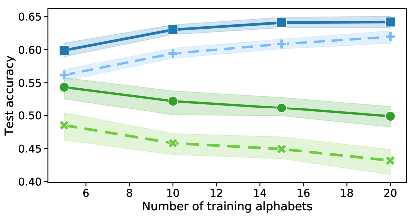
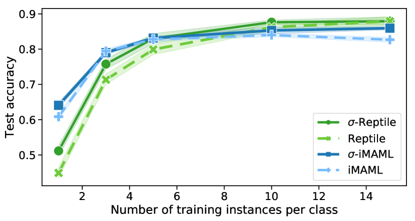
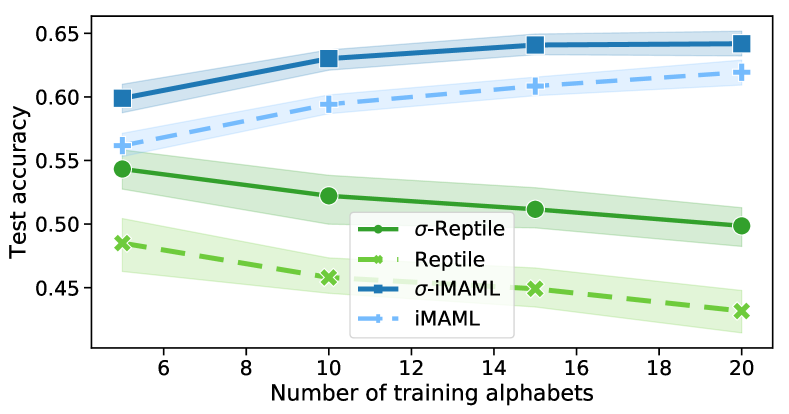
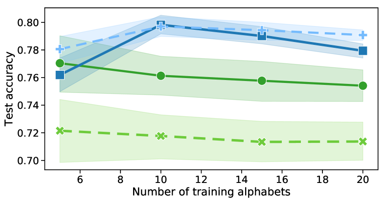
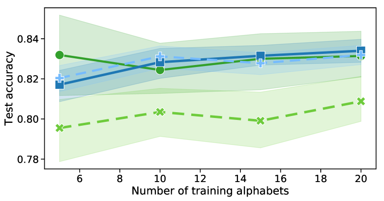
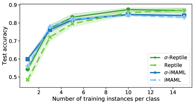
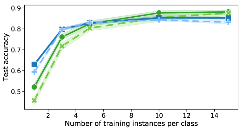
We now reduce the amount of augmentation and data to make the domain more challenging. Fig. 4 shows our results in this small-data regime. Both shrinkage variants significantly improve over their non-shrinkage counterparts when there are few training instances per alphabet. This gap grows as the number of training instances decreases, demonstrating that shrinkage helps prevent overfitting. Interestingly, the Reptile variants begin to outperform the iMAML variants as the number of training instances increases, despite the extra validation data used by the iMAML variants. Results for all combinations of alphabets and instances are shown in the appendix.

Figure 3: Learned $\boldsymbol{\sigma}^{2}$ of WaveNet modules. Every block contains four layers (See Appendix E.2 for details).

$\boldsymbol{\sigma}$-iMAML	$73.6\pm 1.3\%$
iMAML	$72.8\pm 1.2\%$
$\boldsymbol{\sigma}$-Reptile	$78.9\pm 1.2\%$
Reptile	$77.8\pm 1.1\%$

Table 2: Average test accuracy and $95\%$ confidence intervals for $10$ runs on large-data augmented Omniglot.

Figure 4: Mean test accuracy and $95\%$ confidence intervals for $10$ runs on small-data aug. Omniglot as a function of the number of alphabets (left, $1$ image per character) and instances (right, $15$ alphabets).

Text-to-speech sample quality. The state-of-the art approaches for this domain [1] are to finetune either the entire model (aka. SEA-All) or just the speaker embedding (SEA-Emb). We compare these two methods to meta-training with Reptile and $\boldsymbol{\sigma}$-Reptile. We also tried to run $\boldsymbol{\sigma}$-MAML and $\boldsymbol{\sigma}$-iMAML but $\boldsymbol{\sigma}$-MAML ran out of memory with one adaptation step and $\boldsymbol{\sigma}$-iMAML trained too slowly.

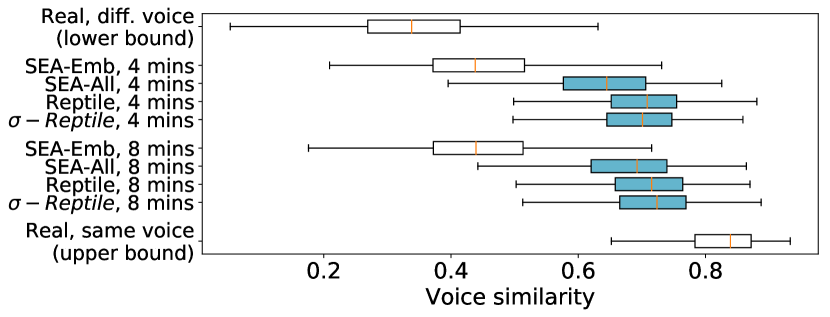
We evaluate the generated sample quality using two voice synthesis metrics: (1) the voice similarity between a sample and real speaker utterances using a speaker verification model [47, 1], and (2) the sample naturalness measured by the mean opinion score (MOS) from human raters. Fig. 5 shows the distribution of sample similarities for each method, along with an upper (lower) bound computed from real utterances between the same (different) speakers. Sample naturalness for each method is shown in Table 3, along with an upper bound created by training the same model on $40$ hours of data.

$\boldsymbol{\sigma}$-Reptile and Reptile clearly outperform SEA-All and SEA-Emb. $\boldsymbol{\sigma}$-Reptile has comparable median similarity with Reptile, and its sample naturalness surpasses Reptile with both 8 minutes of speech data, and 4 minutes, which is less than used in meta-training. Overall, the $\boldsymbol{\sigma}$-Reptile samples have the highest quality despite adapting only $12$ of the $123$ modules. SEA-All and Reptile, which adapt all modules, overfit quickly and underperform, despite adaptation being early-stopped. Conversely, SEA-Emb underfits and does not improve with more data because it only tunes the speaker embedding.

Figure 5: Box-plot of voice similarity measurements from utterances (higher is better).

	4 mins	8 mins
SEA-Emb	$1.51\pm 0.05$	$1.57\pm 0.05$
SEA-All	$1.41\pm 0.04$	$1.73\pm 0.06$
Reptile	$\textbf{1.93}\pm 0.05$	$2.09\pm 0.06$
$\boldsymbol{\sigma}$-Reptile	$\textbf{1.98}\pm 0.06$	$\textbf{2.28}\pm 0.06$
Trained with 40 hours of data (upper bound)	$2.59\pm 0.07$

Table 3: Mean opinion score of sample naturalness. Scores range from 1–5 (higher is better).

5.4 Discussion

We thus answer all three experimental questions in the affirmative. In both image classification and text-to-speech, the learned shrinkage priors correspond to meaningful and interesting task-specific modules. These modules differ between domains, however, indicating that they should be learned from data. Studying these learned modules allows us to discover new or existing knowledge about the behavior of different parts of the network, while adapting only the task-specific modules provides the same performance as adapting all layers. Finally, learning and using our shrinkage prior helps prevent overfitting and improves performance in low-data, long-adaptation regimes.

6 Conclusions

This work proposes a hierarchical Bayesian model for meta-learning that places a shrinkage prior on each module to allow learning the extent to which each module should adapt, without a limit on the adaptation horizon. Our formulation includes MAML, Reptile, and iMAML as special cases, empirically discovers a small set of task-specific modules in various domains, and shows promising improvement in a practical TTS application with low data and long task adaptation. As a general modular meta-learning framework, it allows many interesting extensions, including incorporating alternative Bayesian inference algorithms, modular structure learning, and learn-to-optimize methods.

Broader Impact

This paper presents a general meta-learning technique to automatically identify task-specific modules in a model for few-shot machine learning problems. It reduces the need for domain experts to hand-design task-specific architectures, and thus further democratizes machine learning, which we hope will have a positive societal impact. In particular, general practitioners who can not afford to collect a large amount of labeled data will be able to take advantage of a pre-trained generic meta-model and adapt its task-specific components to a new task based on limited data. One example application might be to adapt a multilingual text-to-speech model to a low-resource language or the dialect of a minority ethnic group.

As a data-driven method, like other machine learning techniques, the task-independent and task-specific modules discovered by our method are based on the distribution of tasks in the meta-training phase. Adaptation may not generalize to a task with characteristics that fundamentally differ from those of the training distribution. Applying our method to a new task without examining the task similarity runs the risk of transferring induced bias from meta-training to the out-of-distribution task. For example, a meta image classification model trained only on vehicles is unlikely to be able to be finetuned to accurately identify a pedestrian based on the adaptable modules discovered during meta-training. To mitigate this problem, we suggest ML practitioners first understand whether the characteristics of the new task match those of the training task distribution before applying our method.

Appendix

This appendix contains the supplementary material for the main text. In Appendix A, we first prove Lemma 1 and then provide a detailed analysis of the introduced estimation approaches on a simple example. In Appendix B, we provide details of the derivation of the implicit gradients in Eqs. 7 and 10, show the equivalence of $\boldsymbol{\sigma}$-iMAML and iMAML when $\sigma_{m}^{2}$ is shared across all modules and fixed, and provide more discussion on the objective introduced in Section 4.2. In Appendix C, we demonstrate the different behavior of approaches that meta-learn the learning rate per module versus our approach that meta-learns the shrinkage prior per module, on two synthetic problems. In Appendix D, we provide additional details about our implementation of the iMAML baseline and our shrinkage algorithms. Finally, in Appendix E, we explain the experiments in more detail, provide information about the setup and hyperparameters, and present additional results.

Appendix A Analysis

In this section, we first prove Lemma 1, which shows in general that it is not feasible to estimate all the parameters $(\boldsymbol{\sigma}^{2},\boldsymbol{\phi},\boldsymbol{\theta}_{1:T})$ jointly by optimizing the joint log-density. We then provide detailed analysis of the properties of the two estimation approaches introduced in Section 4 for a simple hierarchical normal distribution example. Finally, we discuss the pathological behavior when estimating $\boldsymbol{\sigma}^{2}$ from the joint log-density in the same example.

A.1 Maximization of $\log p(\boldsymbol{\theta}_{1:T},\mathcal{D}|\boldsymbol{\sigma}^{2},\boldsymbol{\phi})$

Lemma 1 states that the function $f:(\boldsymbol{\sigma}^{2},\boldsymbol{\phi},\boldsymbol{\theta}_{1:T})\mapsto\log p(\boldsymbol{\theta}_{1:T},\mathcal{D}|\boldsymbol{\sigma}^{2},\boldsymbol{\phi})$ diverges to $+\infty$ as $\boldsymbol{\sigma}\rightarrow 0^{+}$ when $\theta_{t,m}=\boldsymbol{\phi}_{m}$ for all $t\in\{1,...,T\},m\in\{1,...,M\}$. We first establish here this result.

Proof of Lemma 1.

For simplicity, we prove the result for $M=1$ and $N_{t}=N$. The extension to the general case is straightforward. We have

$$\log p(\theta_{1:T},\mathbf{x}_{1:T}|\phi,\sigma^{2})=-\frac{T}{2}\log\sigma^{2}-\frac{1}{2}\sum_{t=1}^{T}\frac{(\theta_{t}-\phi)^{2}}{\sigma^{2}}+\sum_{t=1}^{T}\sum_{i=1}^{N}\log p(x_{t,n}|\theta_{t})\,.$$

From this expression, it is clear that when $\theta_{t}=\phi$ for all $t$, then $\log p(\theta_{1:T},\mathbf{x}_{1:T}|\phi,\sigma^{2})\rightarrow+\infty$ as $\sigma^{2}\rightarrow 0^{+}$. ∎

This shows that the global maximum of $\log p(\theta_{1:T},\mathbf{x}_{1:T}|\phi,\sigma^{2})$ does not exist in general, and thus we should not use this method for estimating $\sigma^{2}$.

This negative result illustrates the need for alternative estimators. In the following sections, we analyze the asymptotic behavior of the estimates of $\boldsymbol{\phi}$ and $\boldsymbol{\sigma}^{2}$ proposed in Section 4 as the number of training tasks $T\rightarrow\infty$ in a simple example. In Section A.2.3, we analyze the behavior of Lemma 1 when optimizing $\log p(\theta_{1:T},\mathbf{x}_{1:T}|\phi,\sigma^{2})$ w.r.t. $\boldsymbol{\sigma}^{2}$ with a local optimizer.

A.2 Analysis of estimates in a simple example

To illustrate the asymptotic behavior of different learning strategies as $T\rightarrow\infty$, we consider a simple model with $M=1$ module, $D_{t}=D=1$ for all tasks and normally distributed observations. We use non-bolded symbols to denote that all variables are scalar in this section.

Example 1 (Univariate normal).

$$M=1,D_{t}=1,N_{t}=N,\forall t=1,\dots,T,$$

$$x_{t,n}\sim{\cal N}(x_{t,n}|\theta_{t},1),\forall t=1,\dots,T,n=1,\dots,N.$$

It follows that

$$p(\theta_{1:T},\mathbf{x}_{1:T}|\phi,\sigma^{2})=\prod_{t=1}^{T}\left({\cal N}(\theta_{t}|\phi,\sigma^{2})\prod_{n=1}^{N}{\cal N}(x_{t,n}|\theta_{t},1)\right)\,,$$ (11)

and we use the notation for the negative joint log-density up to a constant

$$\ell_{\mathrm{joint}}(\theta_{1:T},\phi,\sigma^{2}) =-\log p(\theta_{1:T},\mathbf{x}_{1:T}|\phi,\sigma^{2})$$

$$=\frac{T}{2}\log\sigma^{2}+\frac{1}{2}\sum_{t=1}^{T}\frac{(\theta_{t}-\phi)^{2}}{\sigma^{2}}+\frac{1}{2}\sum_{t=1}^{T}\sum_{n=1}^{N}(x_{t,n}-\theta_{t})^{2}$$

$$=\sum_{t=1}^{T}\ell_{t}^{\text{train}}(\theta_{t},\phi,\sigma^{2})\,.$$ (12)

We also assume there exists a set of independently sampled validation data $\mathbf{y}_{1:T}$ where $y_{t,n}\sim{\cal N}(y|\theta_{t},1)$ for $t\in\{1,\dots,T\},n\in\{1,\dots,K\}$. The corresponding negative log-likelihood given point estimates $\hat{\theta}_{1:T}$ is given up to a constant by

$$\hat{\ell}_{\mathrm{PLL}}=\sum_{t=1}^{T}\ell_{t}^{\text{val}}(\hat{\theta}_{t})=\frac{1}{2}\sum_{t=1}^{T}\sum_{k=1}^{K}(y_{t,k}-\hat{\theta}_{t})^{2}.$$ (13)

We denote by $\phi_{\mathrm{True}}$ and $\sigma_{\mathrm{True}}$ the true value of $\phi$ and $\sigma$ for the data generating process described above.

A.2.1 Estimating $\boldsymbol{\phi}$ and $\boldsymbol{\phi}$ with predictive log-likelihood

We first show that when we estimate $\theta_{t}$ with MAP on $\ell_{t}^{\text{train}}$ and estimate $\phi$ and $\sigma^{2}$ with the predictive log-likelihood as described in Section 4.1, the estimates $\hat{\phi}$ and $\hat{\sigma}^{2}$ are consistent.

Proposition 1.

Let $\hat{\theta}_{t}(\phi,\sigma^{2})=\arg\min_{\theta_{t}}\ell_{t}^{\text{train}}(\theta_{t},\phi,\sigma^{2})$ and define $(\hat{\phi},\hat{\sigma}^{2})=\arg_{\phi,\sigma^{2}}\{\nabla_{(\phi,\sigma^{2})}\hat{\ell}_{\mathrm{PLL}}(\hat{\theta}_{1:T})=0\}$ then, as $T\rightarrow\infty$, we have

$$\hat{\phi}(\hat{\sigma}^{2})\rightarrow\phi_{\mathrm{True}},\quad\hat{\sigma}^{2}\rightarrow\sigma_{\mathrm{True}}^{2},$$

in probability.

Proof.

We denote the sample average

$$\bar{x}_{t}:=\frac{1}{N}\sum_{n,t}x_{n,t},\quad\bar{y}_{t}:=\frac{1}{K}\sum_{k,t}y_{k,t}\,,$$ (14)

and the average over all tasks $\bar{x}=\frac{1}{T}\sum_{t=1}^{T}\bar{x}_{t}$, $\bar{y}=\frac{1}{T}\sum_{t=1}^{T}\bar{y}_{t}$.

The equation $\nabla_{\theta_{t}}\ell_{t}^{\text{train}}=0$ gives

$$\hat{\theta}_{t}(\phi,\sigma^{2})=\frac{\sum_{n=1}^{N}x_{t,n}+\phi/\sigma^{2}}{N+1/\sigma^{2}}=\frac{\bar{x}_{t}+\phi/N\sigma^{2}}{1+1/N\sigma^{2}}.$$ (15)

By plugging Eq. 15 in Eq. 7, it follows that

$$\nabla_{\sigma^{2}}\hat{\ell}_{\mathrm{PLL}} =-\sum_{t}\nabla_{\theta_{t}}\ell_{t}^{\text{val}}(\theta_{t})\mathbf{H}^{-1}_{\theta_{t}\theta_{t}}\mathbf{H}_{\theta_{t}\sigma^{2}}$$

$$=\frac{K}{N\sigma^{4}\left(1+\frac{1}{N\sigma^{2}}\right)}\sum_{t}(\theta_{t}-\bar{y}_{t})(\theta_{t}-\phi)$$

$$=\frac{K}{N\sigma^{4}(1+\frac{1}{N\sigma^{2}})^{3}}\cdot$$

$$\quad\quad\sum_{t}\left(\bar{x}_{t}-\bar{y}_{t}+\frac{1}{N\sigma^{2}}(\phi-\bar{y}_{t})\right)(\bar{x}_{t}-\phi)\,.$$ (16)

We then solve $\nabla_{\sigma^{2}}\hat{\ell}_{\mathrm{PLL}}=0$ as a function of $\phi$,

$$\hat{\sigma}^{2}(\phi)=\frac{\frac{1}{T}\sum_{t}(\bar{x}_{t}-\phi)(\bar{y}_{t}-\phi)}{\frac{N}{T}\sum_{t}(\bar{x}_{t}-\bar{y}_{t})(\bar{x}_{t}-\phi)}.$$ (17)

Similarly, we solve $\nabla_{\phi}\hat{\ell}_{\mathrm{PLL}}(\hat{\theta}_{1:T}(\phi,\sigma^{2})=0$ as

$$\nabla_{\phi}\hat{\ell}_{\mathrm{PLL}} =-\sum_{t}\nabla_{\theta_{t}}\ell_{t}^{\text{val}}(\theta_{t})\mathbf{H}^{-1}_{\theta_{t}\theta_{t}}\mathbf{H}_{\theta_{t}\phi}$$

$$=-\frac{K}{1+N\sigma^{2}}\sum_{t=1}^{T}\left(\bar{y}_{t}-\frac{\bar{x}_{t}+\phi/N\sigma^{2}}{1+1/N\sigma^{2}}\right)=0,$$

this yields

$$\hat{\phi}(\sigma^{2})=\bar{y}+N\sigma^{2}(\bar{y}-\bar{x}).$$ (19)

By combining Eq. 17 to Eq. 19, we obtain

$$\hat{\phi}=\frac{\overline{x(x-y)}\bar{y}+\overline{xy}(\bar{y}-\bar{x})}{\bar{x}(\bar{y}-\bar{x})+\overline{x(x-y)}}$$ (20)

where, for a function $f$ of variable $x,y$, we define $\overline{f(x,y)}:=\frac{1}{T}\sum_{t}f(\bar{x}_{t},\bar{y}_{t})$.

Following the data generating process, the joint distribution of $\bar{x}_{t}$ and $\bar{y}_{t}$ with $\theta_{t}$ integrated out is jointly normal and satisfies

$$[\bar{x}_{t},\bar{y}_{t}]^{T}\sim{\cal N}\left(\phi_{\mathrm{True}}\boldsymbol{1}_{2},\begin{bmatrix}\sigma_{\mathrm{True}}^{2}+\frac{1}{N}&\sigma_{\mathrm{True}}^{2}\\ \sigma_{\mathrm{True}}^{2}&\sigma_{\mathrm{True}}^{2}+\frac{1}{K}\end{bmatrix}\right).$$ (21)

As $T\rightarrow\infty$, it follows from the law of large numbers and Slutsky’s lemma that $\hat{\phi}\rightarrow\phi_{\mathrm{True}}$ in probability. Consequently, it also follows from (17) that $\hat{\sigma}^{2}\rightarrow\sigma^{2}_{\mathrm{True}}$ in probability. ∎

A.2.2 Estimating $\phi$ with MAP and $\sigma^{2}$ with predictive log-likelihood

Alternatively, we can follow the approach described in Section 4.2 to estimate both $\theta_{1:T}$ and $\phi$ with MAP on $\ell_{\mathrm{joint}}$ (Eq. 12), i.e.,

$$(\hat{\phi}(\sigma^{2}),\hat{\theta}_{1:T}(\sigma^{2}))=\arg\max_{(\phi,\theta_{1:t})}\ell_{\mathrm{joint}}(\theta_{1:T},\phi,\sigma^{2})\,,$$ (22)

and estimate $\sigma^{2}$ with the predictive log-likelihood by finding the root of the approximate implicit gradient in Eq. 10.

We first show that given any fixed value of $\sigma^{2}$, the MAP estimate of $\phi$ is consistent.

Proposition 2 (Consistency of MAP estimate of $\phi$).

For any fixed $\sigma>0$, $\hat{\phi}(\sigma^{2})=\bar{x}$, so $\hat{\phi}(\sigma^{2})\rightarrow\phi_{\mathrm{True}}$ in probability as $T\rightarrow\infty$.

Proof of Proposition 2.

The equation $\nabla_{\phi}\ell_{\mathrm{joint}}=0$ for $\ell_{\mathrm{joint}}$ defined in Eq. 12 gives

$$\hat{\phi}(\sigma^{2})=\frac{1}{T}\sum_{t=1}^{T}\hat{\theta}_{t}(\sigma^{2}).$$ (23)

By summing Eq. 15 over $t=1,...,T$ and using Eq. 23, we obtain

$$\hat{\phi}(\sigma^{2}) =\bar{x},\quad\hat{\theta}_{t}(\sigma^{2})=\frac{\bar{x}_{t}+\frac{\bar{x}}{N\sigma^{2}}}{1+\frac{1}{N\sigma^{2}}}.$$ (24)

The distribution of $\bar{x}$ follows directly from Eq. 21. Therefore, $\hat{\phi}(\sigma^{2})$ is unbiased for any $T$ and it is additionally consistent by Chebyshev’s inequality as $T\rightarrow\infty$. ∎

Now we show that estimating $\sigma^{2}$ by finding the roots of the implicit gradient in Eq. 10 is also consistent.

Proposition 3.

Let $(\hat{\phi}(\sigma^{2}),\hat{\theta}_{1:T}(\sigma^{2}))=\arg\max_{(\phi,\theta_{1:T})}\ell_{\mathrm{joint}}(\theta_{1:T},\phi,\sigma^{2})$ and define $\hat{\sigma}^{2}=\arg_{\sigma^{2}}\{\nabla_{\sigma^{2}}\hat{\ell}_{\mathrm{PLL}}(\hat{\theta}_{1:T})=0\}$ where the gradient is defined as in Eq. 10, then, as $T\rightarrow\infty$, we have

$$\hat{\phi}(\hat{\sigma}^{2})\rightarrow\phi_{\mathrm{True}},\quad\hat{\sigma}^{2}\rightarrow\sigma_{\mathrm{True}}^{2},$$

in probability.

Proof.

From Eq. 10, we follow the same derivation as Eq. 17 and get the root of the gradient for $\sigma^{2}$ as a function of $\hat{\phi}$:

$$\hat{\sigma}^{2}(\hat{\phi})=\frac{\frac{1}{T}\sum_{t}(\bar{x}_{t}-\hat{\phi})(\bar{y}_{t}-\hat{\phi})}{\frac{N}{T}\sum_{t}(\bar{x}_{t}-\bar{y}_{t})(\bar{x}_{t}-\hat{\phi})}.$$ (25)

By plugging Eq. 24, it follows from the joint distribution of $(\bar{x}_{t},\bar{y}_{t})$ (Eq. 21), the law of large numbers and Slutsky’s lemma that $\hat{\sigma}^{2}\rightarrow\sigma^{2}_{\mathrm{True}}$ in probability as $T\rightarrow\infty$. ∎

A.2.3 MAP estimate of $\sigma^{2}$

From Lemma 1, we know that maximizing $\ell_{\mathrm{joint}}$ (Eq. 12) w.r.t. $(\theta_{t},\phi,\sigma^{2})$ is bound to fail. Here we show the specific $\sigma^{2}$ estimate one would obtain by following gradient descent on $\ell_{\mathrm{joint}}$ in the running example.

Let $S$ denote the sample variance of $\bar{x}_{t}$ across tasks, that is

$$S=\frac{\sum_{t=1}^{T}(\bar{x}_{t}-\bar{x})^{2}}{T}\,.$$ (26)

We can easily establish from Eq. 21 that

$$S\sim\frac{\sigma_{\mathrm{True}}^{2}+\frac{1}{N}}{T}\chi_{T-1}^{2}\,,$$ (27)

where $\chi_{T-1}^{2}$ is the standard Chi-squared random variable with $T-1$ degrees of freedom. Although $\hat{\phi}(\sigma^{2})$ is consistent whenever $\sigma^{2}>0$, the following proposition shows that maximizing $\ell_{\mathrm{joint}}(\hat{\theta}_{1:T}(\sigma^{2}),\hat{\phi}(\sigma^{2}),\sigma^{2})$ w.r.t. $\sigma^{2}$ remains problematic.

Proposition 4 (Estimation of $\sigma$ by gradient descent).

Minimizing the function $\sigma^{2}\mapsto\ell_{\mathrm{joint}}(\hat{\theta}_{1:T}(\sigma^{2}),\hat{\phi}(\sigma^{2}),\sigma^{2})$ by gradient descent will diverge at $\sigma\rightarrow 0^{+}$ if either of the following two conditions is satisfied

1. $S<\frac{4}{N}$,

2. $\sigma^{2}$ is initialized in $\left(0,\frac{1}{2}\left(S-\frac{2}{N}-\sqrt{S(S-\frac{4}{N})}\right)\right)$.

Otherwise, it converges to a local minimum $\hat{\sigma}^{2}=\frac{1}{2}\left(S-\frac{2}{N}+\sqrt{S(S-\frac{4}{N})}\right)$.

Corollary 1.

As the number of training tasks $T\rightarrow\infty$, condition 1 is equivalent to

$$\sigma_{\mathrm{True}}^{2}<\frac{3}{N}$$

while the upper endpoint of the interval in condition 2 becomes

$$\frac{1}{2}\left(\sigma_{\mathrm{True}}^{2}-\frac{1}{N}-\sqrt{(\sigma_{\mathrm{True}}^{2}+\frac{1}{N})(\sigma_{\mathrm{True}}^{2}-\frac{3}{N})}\right)\,,$$

beyond which the $\sigma^{2}$ estimate converges to

$$\hat{\sigma}^{2}=\frac{1}{2}\left(\sigma_{\mathrm{True}}^{2}-\frac{1}{N}+\sqrt{(\sigma_{\mathrm{True}}^{2}+\frac{1}{N})(\sigma_{\mathrm{True}}^{2}-\frac{3}{N})}\right)\,.$$ (28)

Proofs of Proposition 4 and Corollary 1.

It follows from Eq. 24 that

$$\hat{\theta}_{t}(\sigma)-\hat{\phi}(\sigma) =\frac{\bar{x}_{t}-\bar{x}}{1+\frac{1}{N\sigma^{2}}}.$$ (29)

By solving $\nabla_{\sigma^{2}}\ell_{\mathrm{joint}}=0$, we obtain

$$\hat{\sigma}^{2}=\frac{\sum_{t=1}^{T}(\theta_{t}-\phi)^{2}}{T}.$$ (30)

Plugging Eq. 29 into this expression yields

$$\hat{\sigma}^{2}=\frac{\sum_{t=1}^{T}(\bar{x}_{t}-\bar{x})^{2}}{T(1+\frac{1}{N\hat{\sigma}^{2}})^{2}}=\frac{S}{(1+\frac{1}{N\hat{\sigma}^{2}})^{2}}.$$ (31)

Hence, by rearranging this expression, we obtain the following quadratic equation for $\hat{\sigma}^{2}$

$$\hat{\sigma}^{4}+(2/N-S)\hat{\sigma}^{2}+1/N^{2}=0.$$ (32)

Positive roots of Eq. 32 exist if and only if

$$S\geq\frac{4}{N}.$$ (33)

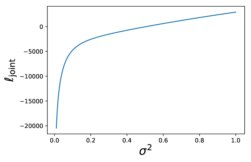
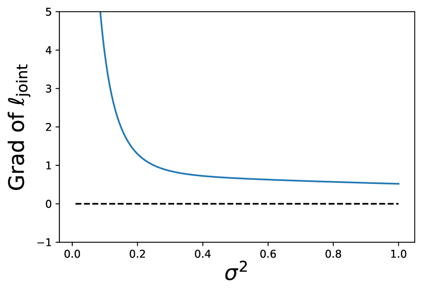
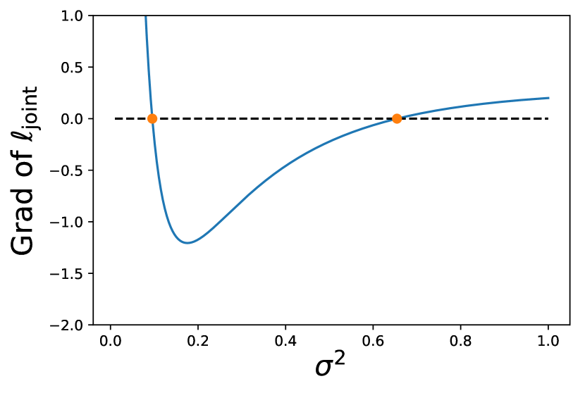
When condition (33) does not hold, no stationary point exists and gradient descent from any initialization will diverge toward $\hat{\sigma}^{2}\rightarrow 0^{+}$ as it can be checked that $\nabla_{\sigma^{2}}\ell_{\mathrm{joint}}<0$. Figs. 6(a) and 6(c) illustrate $\ell_{\mathrm{joint}}$ and $\nabla_{\sigma^{2}}\ell_{\mathrm{joint}}$ as a function of $\sigma^{2}$ in this case.

When the condition above is satisfied, there exist two (or one when $S=4/N$, an event of zero probability) roots at:

$$\sigma_{\mathrm{root}}^{2} =\frac{1}{2}\left(S-\frac{2}{N}\pm\sqrt{S(S-\frac{4}{N})}\right).$$ (34)

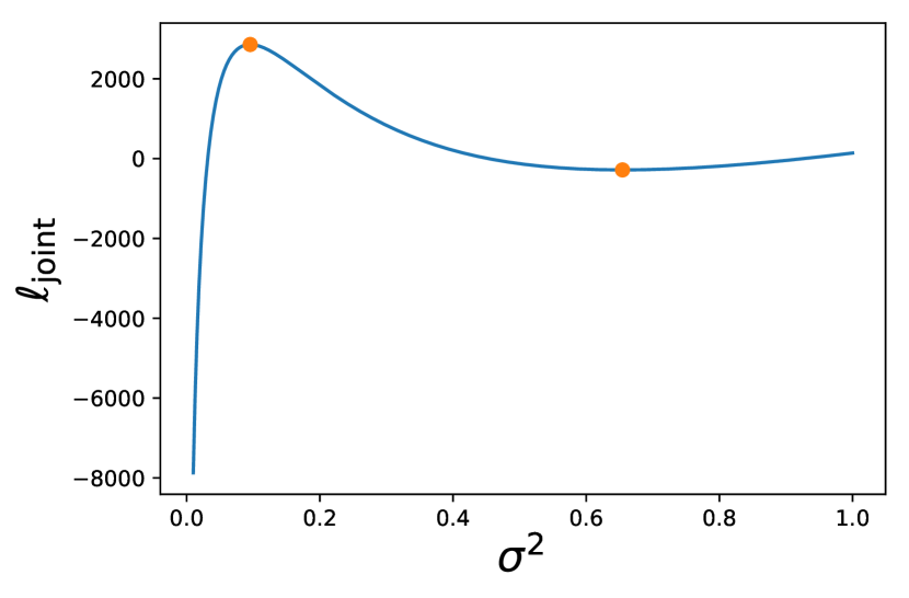
By checking the sign of the gradient $\nabla_{\sigma^{2}}\ell_{\mathrm{joint}}$ and plugging it in to Eq. 29, we find that the left root is a local maximum and the right root is a local minimum. So if one follows gradient descent to estimate $\sigma^{2}$, it will converge towards $0^{+}$ when $\sigma^{2}$ is initialized below the left root and to the second root otherwise. Figs. 6(b) and 6(d) illustrate the function of $\ell_{\mathrm{joint}}$ and its gradient as a function of $\sigma^{2}$ when $\phi$ and $\theta_{t}$ are at their stationary point and condition 1 is satisfied.

To prove the corollary, we note that it follows from Eq. 21 that $S\rightarrow\sigma_{\mathrm{True}}^{2}+\frac{1}{N}$ as $T\rightarrow\infty$. Hence the condition Eq. 33 approaches

$$\sigma_{\mathrm{True}}^{2}\geq\frac{3}{N}.$$ (35)

Similarly, when $T\rightarrow\infty$, Eq. 35 becomes

$$\sigma_{\mathrm{root}}^{2} =\frac{1}{2}\left(\sigma_{\mathrm{True}}^{2}-\frac{1}{N}\pm\sqrt{(\sigma_{\mathrm{True}}^{2}+\frac{1}{N})(\sigma_{\mathrm{True}}^{2}-\frac{3}{N})}\right).$$ (36)

∎

(a) $\ell_{\mathrm{joint}}(\sigma^{2})$ when stationary points do not exist.

(b) $\ell_{\mathrm{joint}}(\sigma^{2})$ when stationary points exist.

(c) $\nabla_{\sigma^{2}}\ell_{\mathrm{joint}}$ when stationary points do not exist.

(d) $\nabla_{\sigma^{2}}\ell_{\mathrm{joint}}$ when stationary points exist.

Figure 6: Example of $\ell_{\mathrm{joint}}(\sigma^{2})$ up to a constant, and its gradient w.r.t. $\sigma^{2}$. Orange dots denote stationary points.

Appendix B Derivation of the approximate gradient of predictive log-likelihood in Section 4

B.1 Implicit gradient of $\boldsymbol{\sigma}$-iMAML in Eq. 7

Lemma 2.

(Implicit differentiation) Let $\hat{\mathbf{y}}(\mathbf{x})$ be the stationary point of function $f(\mathbf{x},\mathbf{y})$, i.e. $\nabla_{\mathbf{y}}f(\mathbf{x},\mathbf{y})|_{\mathbf{y}=\hat{\mathbf{y}}(\mathbf{x})}=0~{}\forall\mathbf{x}$, then the gradient of $\hat{\mathbf{y}}$ w.r.t. $\mathbf{x}$ can be computed as

$$\nabla_{\mathbf{x}}\hat{\mathbf{y}}(\mathbf{x})=-(\nabla_{\mathbf{y}\mathbf{y}}^{2}f)^{-1}\nabla_{\mathbf{y}\mathbf{x}}^{2}f.$$ (37)

By applying the chain rule, the gradient of the approximate predictive log-likelihood $\ell_{t}^{\text{val}}(\hat{\boldsymbol{\theta}}_{t})$ (from Eq. 5) w.r.t. the meta variables $\boldsymbol{\Phi}=(\boldsymbol{\sigma}^{2},\boldsymbol{\phi})$ is given by

$$\nabla_{\boldsymbol{\Phi}}\ell_{t}^{\text{val}}(\hat{\boldsymbol{\theta}}_{t}(\boldsymbol{\Phi}))=\nabla_{\hat{\boldsymbol{\theta}}_{t}}\ell_{t}^{\text{val}}(\hat{\boldsymbol{\theta}}_{t})\nabla_{\boldsymbol{\Phi}}\hat{\boldsymbol{\theta}}_{t}(\boldsymbol{\Phi})\,.$$ (38)

Applying Lemma 2 to the joint log-density on the training subset in Eq. 4, $\ell_{t}^{\text{train}}(\boldsymbol{\theta}_{t},\boldsymbol{\Phi})$. We have

$$\nabla_{\boldsymbol{\Phi}}\hat{\boldsymbol{\theta}}_{t}(\boldsymbol{\Phi})=-\left(\nabla^{2}_{\boldsymbol{\theta}_{t}\boldsymbol{\theta}_{t}}\ell_{t}^{\text{train}}\right)^{-1}\nabla^{2}_{\boldsymbol{\theta}_{t}\boldsymbol{\Phi}}\ell_{t}^{\text{train}}.$$ (39)

Plug the equation above to Eq. 38 and we obtain the implicit gradient of $\ell_{t}^{\text{val}}$ in Eq. 7.

B.2 Equivalence between $\boldsymbol{\sigma}$-iMAML and iMAML when $\boldsymbol{\sigma}_{m}^{2}$ is constant

When all modules share a constant variance, $\sigma_{m}^{2}\equiv\sigma^{2}$, we expand the log-prior term for task parameters $\boldsymbol{\theta}_{t}$ in $\ell_{t}^{\text{train}}$ (4) and plug in the normal prior assumption as follows,

$$\log p(\boldsymbol{\theta}_{t}|\boldsymbol{\sigma}^{2},\boldsymbol{\phi}) =\sum_{m=1}^{M}\bigg{(}-\frac{D_{m}}{2}\log(2\pi\sigma_{m}^{2})-\frac{\|\boldsymbol{\theta}_{mt}-\boldsymbol{\phi}_{m}\|^{2}}{2\sigma_{m}^{2}}\bigg{)}$$

$$=-\frac{D}{2}\log(2\pi\sigma^{2})-\frac{\|\boldsymbol{\theta}_{t}-\boldsymbol{\phi}\|^{2}}{2\sigma^{2}}.$$ (40)

By plugging the equation above to Eq. 7, we obtain the update for $\boldsymbol{\phi}$ as

$$\Delta_{t}^{\text{$\boldsymbol{\sigma}${}-iMAML{}}} =\nabla_{\boldsymbol{\theta}_{t}}\ell_{t}^{\text{val}}(\boldsymbol{\theta}_{t})\left(\frac{1}{\sigma^{2}}\mathbf{I}-\nabla^{2}_{\boldsymbol{\theta}_{t}\boldsymbol{\theta}_{t}}\log p(\mathcal{D}_{t}^{\text{train}}|\boldsymbol{\theta}_{t})\right)^{-1}\frac{1}{\sigma^{2}}\mathbf{I}$$

$$=\nabla_{\boldsymbol{\theta}_{t}}\ell_{t}^{\text{val}}(\boldsymbol{\theta}_{t})\left(\mathbf{I}-\sigma^{2}\nabla^{2}_{\boldsymbol{\theta}_{t}\boldsymbol{\theta}_{t}}\log p(\mathcal{D}_{t}^{\text{train}}|\boldsymbol{\theta}_{t})\right)^{-1}.$$ (41)

This is equivalent to the update of iMAML by defining the regularization scale $\lambda=1/\sigma^{2}$ and plugging in the definition of $\ell_{t}^{\text{train}}:=-\log p(\mathcal{D}_{t}^{\text{train}}|\boldsymbol{\theta}_{t})$ in Section 2.

B.3 Discussion on the alternative procedure for Bayesian parameter learning (Section 4.2)

By plugging the MAP of $\boldsymbol{\phi}$ (Eq. 9) into Eq. 8 and scaling by $1/T$, we derive the approximate predictive log-likelihood as

$$\hat{\ell}_{\mathrm{PLL}}(\boldsymbol{\sigma}^{2})=\frac{1}{T}\sum_{t=1}^{T}\ell_{t}^{\text{val}}(\hat{\boldsymbol{\theta}}_{t}(\boldsymbol{\sigma}^{2})).$$ (42)

It is a sensible strategy to estimate both the task parameters $\boldsymbol{\theta}_{1:T}$ and the prior center $\boldsymbol{\phi}$ with MAP on the training joint log-density and estimate the prior variance $\boldsymbol{\sigma}^{2}$ on the predictive log-likelihood. If $\hat{\boldsymbol{\phi}}(\boldsymbol{\sigma}^{2})\rightarrow\bar{\boldsymbol{\phi}}(\boldsymbol{\sigma}^{2})$ as $T\rightarrow\infty$ we can think of both $\ell_{\mathrm{PLL}}(\boldsymbol{\sigma}^{2})$ and $\hat{\ell}_{\mathrm{PLL}}(\boldsymbol{\sigma}^{2})$ as approximations to

$$\tilde{\ell}_{\mathrm{PLL}}(\boldsymbol{\sigma}^{2})=-\frac{1}{T}\sum_{t=1}^{T}\log p(\mathcal{D}_{t}^{\text{val}}|\mathcal{D}_{t}^{\text{train}},\bar{\boldsymbol{\phi}}(\boldsymbol{\sigma}^{2}),\boldsymbol{\sigma}^{2}),$$ (43)

which, for $(\mathcal{D}_{t}^{\text{train}},\mathcal{D}_{t}^{\text{val}})\overset{\textrm{i.i.d.}}{\sim}\nu$, converges by the law of large numbers as $T\rightarrow\infty$ towards

$$\tilde{\ell}_{\mathrm{PLL}}(\boldsymbol{\sigma}^{2})\rightarrow-\mathbb{E}_{\nu(\mathcal{D}_{t}^{\text{train}},\mathcal{D}_{t}^{\text{val}})}[\log p(\mathcal{D}_{t}^{\text{val}}|\mathcal{D}_{t}^{\text{train}},\bar{\boldsymbol{\phi}}(\boldsymbol{\sigma}^{2}),\boldsymbol{\sigma}^{2})].$$ (44)

Similarly to Eq. 3, it can be shown that minimizing the r.h.s. of Eq. 42 is equivalent to minimizing the average KL

$$\mathbb{E}_{\nu(\mathcal{D}_{t}^{\text{train}})}[\textrm{KL}(\nu(\mathcal{D}_{t}^{\text{val}}|\mathcal{D}_{t}^{\text{train}})||p\left(\mathcal{D}_{t}^{\text{val}}|\mathcal{D}_{t}^{\text{train}},\bar{\boldsymbol{\phi}}(\boldsymbol{\sigma}^{2}),\boldsymbol{\sigma}^{2}\right))].$$ (45)

B.4 Meta update of $\boldsymbol{\sigma}$-Reptile in Eq. 10

The meta update for $\boldsymbol{\phi}$ can then be obtained by differentiating (9) with respect to $\boldsymbol{\phi}$.

To derive the gradient of Eq. 42 with respect to $\boldsymbol{\sigma}$, notice that when $\boldsymbol{\phi}$ is estimated as the MAP on the training subsets of all tasks, it becomes a function of $\boldsymbol{\sigma}^{2}$. Denote by $\ell^{\mathrm{joint}}(\boldsymbol{\Theta},\boldsymbol{\sigma}^{2})$ the objective in Eq. 9 where $\boldsymbol{\Theta}=(\boldsymbol{\theta}_{1:T},\boldsymbol{\phi})$ is the union of all task parameters $\boldsymbol{\theta}_{t}$ and the prior central $\boldsymbol{\phi}$. It requires us to apply the implicit function theorem to $\ell^{\mathrm{joint}}(\boldsymbol{\Theta},\boldsymbol{\sigma}^{2})$ in order to compute the gradient of the approximate predictive log-likelihood w.r.t. $\boldsymbol{\sigma}^{2}$. However, the Hessian matrix $\nabla^{2}_{\boldsymbol{\Theta},\boldsymbol{\Theta}}\ell^{\mathrm{joint}}$ has a size of $D(T+1)\times D(T+1)$ where $D$ is the size of a model parameter $\boldsymbol{\theta}_{t}$, which becomes too expensive to compute when $T$ is large.

Instead, we take an approximation and ignore the dependence of $\hat{\boldsymbol{\phi}}$ on $\boldsymbol{\sigma}^{2}$. Then $\boldsymbol{\phi}$ becomes a constant when computing $\nabla_{\boldsymbol{\sigma}^{2}}\hat{\boldsymbol{\theta}}_{t}(\boldsymbol{\sigma}^{2})$, and the derivation in Section B.1 applies by replacing $\boldsymbol{\Phi}$ with $\boldsymbol{\sigma}^{2}$, giving the implicit gradient in Eq. 10.

Appendix C Synthetic Experiments to Compare MAML, Meta-SGD and Shrinkage

In this section, we demonstrate the difference in behavior between learning the learning rate per module and learning the shrinkage prior per module on two synthetic few-shot learning problems.

In the first experiment we show that when the number of task adaptation steps in meta-training is sufficiently large for task parameters to reach convergence, meta-learning the learning rate per module has a similar effect as shrinkage regularization when evaluated at the same adaptation step in meta-testing; however, this does not generalize to other adaptation horizons. In the second experiment, when the required number of adaptation steps is longer than meta-training allows, the learned learning rate is determined by the local curvature of the task likelihood function whereas the learned shrinkage variance is determined by task similarity from the data generation prior. Grouping parameters with similar learned learning rates or variances then induces different “modules,” which correspond to different aspects of the meta-learning problem (namely, adaptation curvature vs. task similarity).

We compare the following three algorithms:

1. vanilla MAML[13]: does not have modular modeling; learns the initialization and uses a single learning rate determined via hyper-parameter search.

2. Meta-SGD[30]: learns the initialization as well as a separate learning rate for each parameter.

3. $\boldsymbol{\sigma}$-Reptile: learns the initialization and prior variance $\sigma_{m}^{2}$ for each module.

We run each algorithm on two few-shot learning problems, both of which have the same hierarchical normal data generation process:

$$\boldsymbol{\theta}_{m,t} \sim{\cal N}(\boldsymbol{\theta}_{m,t}|\boldsymbol{\phi}_{m},\sigma_{m}^{2}),$$

$$\mathbf{x}_{t,n} \sim{\cal N}(\mathbf{x}_{t,n}|\boldsymbol{\mu}(\boldsymbol{\theta}_{t}),\Xi)\,,$$

for each latent variable dimension $m$, task $t$, and data point $n$. The hyper-parameters $\boldsymbol{\phi}$ and $\boldsymbol{\sigma}^{2}$ are shared across all tasks but unknown, and each parameter dimension $\theta_{m}$ has different prior variance, $\sigma_{m}^{2}$. For simplicity, we let every parameter dimension $m$ correspond to one module for Meta-SGD and $\boldsymbol{\sigma}$-Reptile. The $n$-th observation $\mathbf{x}_{t,n}$ for task $t$ is sampled from a Gaussian distribution. The mean is a known function of task parameter $\boldsymbol{\theta}$. The observation noise variance $\Xi=\text{diag}(\boldsymbol{\xi}^{2})=\text{diag}(\xi_{1}^{2},\dots,\xi_{D}^{2})$ is a fixed and known diagonal matrix. The difference between the two problems is that $\boldsymbol{\mu}$ is a linear function of $\boldsymbol{\theta}_{t}$ in the first problem and non-linear in the second.

The task is few-shot density estimation, that is, to estimate the parameters $\boldsymbol{\theta}_{\tilde{t}}$ of a new task $\mathcal{T}_{\tilde{t}}$ given a few observations $\{\mathbf{x}_{\tilde{t},n}\}$, where $N_{t}^{\text{train}}=N_{t}^{\text{val}}$ for all tasks. To understand the behavior of different algorithms under different task loss landscapes we examine different transformation functions $\boldsymbol{\mu}$.

Note that the data generation process matches the Bayesian hierarchical model of shrinkage and thus $\boldsymbol{\sigma}$-Reptile may have an advantage in terms of predictive performance. However, the main purpose of this section is to demonstrate the behavior of these approaches and not to focus on which performs better in this simple task.

For each method, we use gradient descent for task adaptation to optimize the training loss (negative log-likelihood), and then evaluate the generalization loss on holdout tasks. MAML meta-learns the initialization of TaskAdapt, $\boldsymbol{\phi}$, while Meta-SGD meta-learns both $\boldsymbol{\phi}$ and a per-parameter learning rate $\alpha_{m}$, and $\boldsymbol{\sigma}$-Reptile meta-learns the shrinkage prior mean $\boldsymbol{\phi}$ and per-parameter variance $\boldsymbol{\sigma}_{m}^{2}$. Hyperparameters for each algorithm (i.e., learning rates, number of adaptation steps, and initial values of $\boldsymbol{\sigma}$) were chosen by extensive random search. We chose the values that minimized the generalization loss in meta-test. Because the model is small, we are able to run MAML and Meta-SGD for up to 200 task adaptation steps.

C.1 Experiment 1: Linear transformation

(a) Illustration of the hierarchical normal distribution with linear $\mu$.

(b) Generalization loss in meta-testing.

Figure 7: Experiment 1: Linear transform.

Figure 8: Mean absolute error of the estimate of each parameter as a function of task adaptation step.

We begin with a simple model – a joint normal posterior distribution over $\boldsymbol{\theta}_{t}$ with parameters

$$M= 8,$$

$$D= 9,$$

$$\boldsymbol{\phi}= \boldsymbol{1}_{M},$$

$$\boldsymbol{\sigma}= [8,8,8,8,2,2,2,2],$$

$$\boldsymbol{\xi}= [8,8,8,8,5,5,5,5,1],$$

and transformation

$$\boldsymbol{\mu}(\boldsymbol{\theta}_{t})=[\mathbf{I}_{M},\nicefrac{{\boldsymbol{1}_{M}}}{{\sqrt{M}}}]^{\top}\boldsymbol{\theta}_{t}.$$

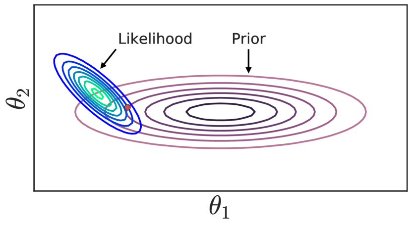
The mean of the observations is thus $\boldsymbol{\theta}$ in the first $M$ dimensions and $\tfrac{1}{\sqrt{M}}\sum_{m}\theta_{m}$ in the final dimension. To make each task nontrivial, we let $\boldsymbol{\xi}$ be small in the final dimension (i.e., $\xi_{M}$ is small) so that the posterior of $\boldsymbol{\theta}$ is restricted to a small subspace near the $\sum_{m}\theta_{m}=\frac{\sqrt{M}}{N_{t}^{\text{train}}}\sum_{n}x_{t,n}$ hyperplane. Gradient descent thus converges slowly regardless of the number of observations. Fig. 7(a) shows an example of this model for the first two dimensions.

Clearly, there are two distinct modules, $\boldsymbol{\theta}_{1:4}$ and $\boldsymbol{\theta}_{5:8}$ but, in this experiment, we do not give the module structure to the algorithms and instead treat each dimension as a separate module. This allows us to evaluate how well the algorithms can identify the module structure from data.

Note that for every task the loss function is quadratic and its Hessian matrix is constant in the parameter space. It is therefore an ideal situation for Meta-SGD to learn an optimal preconditioning matrix (or learning rate per dimension).

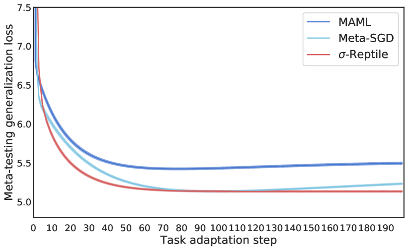
Fig. 7(b) shows the generalization loss on meta-testing tasks. With the small number of observations for each task, the main challenge in this task is overfitting. Meta-SGD and $\boldsymbol{\sigma}$-Reptile obtain the same minimum generalization loss, and both are better than the non-modular MAML algorithm. Importantly, Meta-SGD reaches the minimum loss at step 95, which is the number of steps in meta-training, and then begins to overfit. In contrast, $\boldsymbol{\sigma}$-Reptile does not overfit due to its learned regularization.

Fig. 8 further explains the different behavior of the three algorithms. The mean absolute error (MAE) for each of the 8 parameter dimensions is shown as a function of task adaptation step. MAML shares a single learning rate for all parameters, and thus begins to overfit in different dimensions at different steps, resulting in worse performance. Meta-SGD is able to learn two groups of learning rates, one per each ground-truth module. It learns to coordinate the two learning rates so that they reach the lowest error at the same step, after which it starts to overfit. The learning rate is limited by the curvature enforced by the last observation dimension. $\boldsymbol{\sigma}$-Reptile shares a single learning rate so the error of every dimension drops at about the same speed initially and each dimension reaches its minimum at different steps. It learns two groups of variances so that all parameters are properly regularized and maintain their error once converged, instead of overfitting.

C.2 Experiment 2: Nonlinear transform.

(a) Illustration of the hierarchical normal distribution with non-linear $\mu$.

(b) Generalization loss in meta-testing.

Figure 9: Experiment 2: Nonlinear spiral transform.

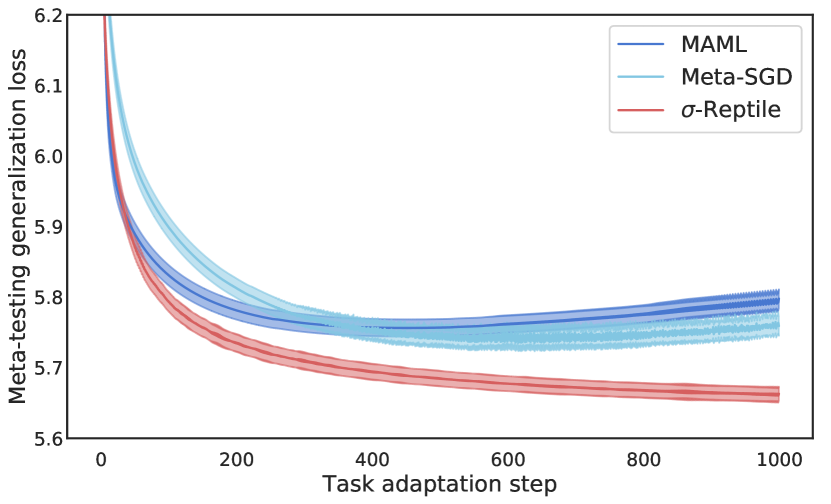
In the second experiment, we explore a more challenging optimization scenario where the mean is a nonlinear transformation of the task parameters. Specifically,

$$M= 10,$$

$$D= 10,$$

$$\boldsymbol{\sigma}= [4,4,4,4,4,4,4,4,8,8],$$

$$\boldsymbol{\phi}= 2\cdot\boldsymbol{1}_{M},$$

$$\boldsymbol{\xi}= 10\cdot\boldsymbol{1}_{D}.$$

The true modules are $\boldsymbol{\theta}_{1:8}$ and $\boldsymbol{\theta}_{9:10}$. The transformation $\boldsymbol{\mu}_{t}(\boldsymbol{\theta}_{t})$ is a “swirl” effect that rotates non-overlapping pairs of consecutive parameters with an angle proportional to their $L_{2}$ distance from the origin. Specifically, each consecutive non-overlapping pair $(\mu_{t,d},\mu_{t,d+1})$ is defined as

$$\begin{bmatrix}\mu_{t,d}\\ \mu_{t,d+1}\end{bmatrix} =\mathrm{Rot}\left(\omega\sqrt{\theta_{t,d}^{2}+\theta_{t,d+1}^{2}}\right)\cdot\begin{bmatrix}\theta_{t,d}\\ \theta_{t,d+1}\end{bmatrix},\quad\text{for~{}~{}}d=1,3,...,M-1,$$

where

$$\mathrm{Rot}(\varphi)=\begin{bmatrix}\cos\varphi&-\sin\varphi\\ \sin\varphi&\cos\varphi\\ \end{bmatrix},$$ (46)

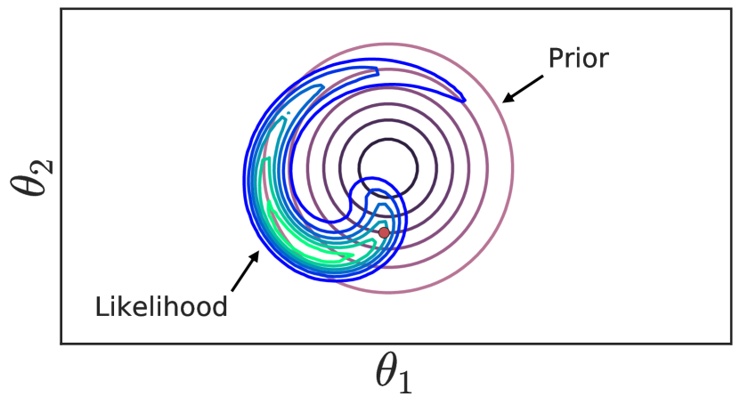
and $\omega=\nicefrac{{\pi}}{{5}}$ is the angular velocity of the rotation. This is a nonlinear volume-preserving mapping that forms a spiral in the observation space. Fig. 9(a) shows an example of the prior and likelihood function in $2$-dimensions of the parameter space.

Compared to the previous example, this highly nonlinear loss surface with changing curvature is more realistic. First-order optimizers are constrained by the narrow valley formed by the “swirly” likelihood function, and thus all algorithms require hundreds of adaptation steps to minimize the loss.

In this case, the best per-parameter learning rate learned by Meta-SGD is restricted by the highest curvature in the likelihood function along the optimization trajectory. In contrast, the optimal per-parameter variance estimated by $\boldsymbol{\sigma}$-Reptile depends on the prior variance $\sigma_{m}^{2}$ in the data generating process, regardless of the value of $\omega$, given that optimization eventually converges.

As a consequence, Meta-SGD and $\boldsymbol{\sigma}$-Reptile exhibit very different behaviors in their predictive performance in Fig. 9(b). Meta-SGD overfits after about 700 steps, while $\boldsymbol{\sigma}$-Reptile keeps improving after 1000 steps.

Also, because MAML and Meta-SGD require backpropagation through the adaptation process, when the number of adaptations steps is higher than 100, we notice that meta-training becomes unstable. As a result, the best MAML and Meta-SGD hyperparameter choice has fewer than 100 adaptation steps in meta-training. These methods then fail to generalize to the longer optimization horizon required in this problem.

We do not show the per-parameter MAE trajectory as in the previous section because this optimization moves through a spiraling, highly coupled trajectory in the parameter space, and thus per-parameter MAE is not a good metric to measure the progress of optimization.

Appendix D Algorithm Implementation Details

D.1 Implementation details for iMAML

In this work, we implement and compare our algorithm to iMAML-GD — the version of iMAML that uses gradient descent within task adaptation [3, Sec. 4] — as this better matches the proximal gradient descent optimizer used in our shrinkage algorithms.

In our implementation of conjugate gradient descent, to approximate the inverse Hessian we apply a damping term following Rajeswaran et al. [3] and restrict the number of conjugate gradient steps to 5 for numerical stability. The meta update is then

$$\Delta_{t}^{\text{iMAML}}=\Big{(}(1+d)\mathbf{I}+\tfrac{1}{\lambda}\nabla^{2}_{\boldsymbol{\theta}_{t}}\ell_{t}^{\text{train}}(\boldsymbol{\theta}_{t})\Big{)}^{-1}\nabla_{\boldsymbol{\theta}_{t}}\ell_{t}^{\text{val}}(\boldsymbol{\theta}_{t}),$$ (47)

where $d$ is the damping coefficient. We treat $d$ and the number of conjugate gradient steps as hyperparameters and choose values using hyperparameter search.

D.2 Implementation details for shrinkage prior algorithms

As in iMAML, we apply damping to the Hessian matrix when running conjugate gradient descent to approximate the product $\nabla_{\boldsymbol{\theta}_{t}}\ell_{t}^{\text{val}}(\hat{\boldsymbol{\theta}}_{t})\mathbf{H}_{\hat{\boldsymbol{\theta}}_{t}\hat{\boldsymbol{\theta}}_{t}}^{-1}$ in $\boldsymbol{\sigma}$-iMAML (Eq. 7) and $\boldsymbol{\sigma}$-Reptile (Eq. 10),

$$\mathbf{H}_{\hat{\boldsymbol{\theta}}_{t}\hat{\boldsymbol{\theta}}_{t}}=-\tilde{d}\mathbf{I}-\boldsymbol{\Sigma}^{-1}-\nabla_{\hat{\boldsymbol{\theta}}_{t}\hat{\boldsymbol{\theta}}_{t}}\log p\left(\mathcal{D}_{t}^{\text{train}}|\boldsymbol{\theta}_{t}\right),$$ (48)

where $\boldsymbol{\Sigma}=\mathrm{Diag}(\sigma_{1}^{2}\mathbf{I}_{D_{1}},\sigma_{2}^{2}\mathbf{I}_{D_{2}},\dots,\sigma_{M}^{2}\mathbf{I}_{D_{M}})$, and $\mathrm{Diag}(\dots,\mathbf{B}_{m},\dots)$ denotes a block diagonal matrix with $m$-th block $\mathbf{B}_{m}$. Note that the damped update rule reduces to that of iMAML when $\sigma_{m}^{2}=1/\lambda,\forall m$ and $\tilde{d}=d\lambda$.

Additionally, we apply a diagonal pre-conditioning matrix in the same structure as $\boldsymbol{\Sigma}$, $\mathbf{P}=\mathrm{Diag}(p_{1}\mathbf{I}_{D_{1}},p_{2}\mathbf{I}_{D_{2}},\dots,p_{M}\mathbf{I}_{D_{M}})$ with $p_{m}=\max\{\sigma_{m}^{-2}/10^{3},1\}$ to prevent an ill-conditioned Hessian matrix when the prior variance becomes small (strong prior).

We also clip the value of $\sigma_{m}^{2}$ to be in $[10^{-5},10^{5}]$. This clipping improves the stability of meta learning, and the range is large enough to not affect the MAP estimate of $\hat{\boldsymbol{\theta}}_{t}$.

Finally, we incorporate a weak regularizer on the shrinkage variance to encourage sparsity in the discovered adaptable modules. The regularized objective for learning $\boldsymbol{\sigma}^{2}$ becomes

$$\frac{1}{T}\ell_{\mathrm{PLL}}+\beta\log\mathrm{IG}(\boldsymbol{\sigma}^{2})\,,$$ (49)

where $\mathrm{IG}$ is the inverse Gamma distribution with shape $\alpha=1$ and scale $\beta$. Unless otherwise stated, we use $\beta=10^{-5}$ for sinusoid and image experiments, and $\beta=10^{-7}$ for text-to-speech experiments. We find that this regularization simply reduces the learned $\sigma_{m}^{2}$ of irrelevant modules without affecting generalization performance.

D.3 Proximal Gradient Descent and Proximal Adam with L2 regularization

The pseudo-code of Proximal Gradient Descent [45] with an L2 regularization is presented in Algorithm 2. We also modify the Adam optimizer [46] to be a proximal method and present the pseudo-code in Algorithm 3.

Input: Parameter $\boldsymbol{\theta}_{t}$, gradient $\mathbf{g}_{t}$, step size $\alpha_{t}$, regularization center $\boldsymbol{\phi}$, L2 regularization scale $\lambda$.

$\boldsymbol{\theta}_{t+\frac{1}{2}}=\boldsymbol{\theta}_{t}-\alpha_{t}\mathbf{g}_{t}$

$\boldsymbol{\theta}_{t+1}=(\boldsymbol{\theta}_{t+\frac{1}{2}}-\boldsymbol{\phi})/(1+\lambda\alpha_{t})+\boldsymbol{\phi}$

return $\boldsymbol{\theta}_{t+1}$

Algorithm 2 Proximal Gradient Descent with L2 Regularization.

Input: Parameter $\boldsymbol{\theta}_{t}$, gradient $\mathbf{g}_{t}$, step size $\alpha_{t}$, regularization center $\boldsymbol{\phi}$, L2 regularization scale $\lambda$, $\epsilon$ for Adam.

$\boldsymbol{\theta}_{t+\frac{1}{2}},\hat{\mathbf{v}}_{t+1}=\mathrm{Adam}(\boldsymbol{\theta}_{t},\mathbf{g}_{t},\alpha_{t})$

$\boldsymbol{\theta}_{t+1}=(\boldsymbol{\theta}_{t+\frac{1}{2}}-\boldsymbol{\phi})/(1+\lambda\alpha_{t}/\sqrt{\hat{\mathbf{v}}_{t+1}+\epsilon})+\boldsymbol{\phi}$

return $\boldsymbol{\theta}_{t+1}$

Algorithm 3 Proximal Adam with L2 Regularization.

Appendix E Experiment Details and Additional Short Adaptation Experiments

In our experiments, we treat each layer (e.g., the weights and bias for a convolutional layer are a single layer) as a module, including batch-normalization layers which we adapt as in previous work [13]. Other choices of modules are straightforward but we leave exploring these for future work. For the chosen hyperparameters, we perform a random search for each experiment and choose the setting that performs best on validation data.

E.1 Augmented Omniglot experiment details

We follow the many-shot Omniglot protocol of Flennerhag et al. [4], which takes the $46$ Omniglot alphabets that have $20$ or more character classes and creates one $20$-way classification task for each alphabet by sampling $20$ character classes from that alphabet. These classes are then kept fixed for the duration of the experiment. Of the $46$ alphabets, $10$ are set aside as a held-out test set, and the remainder are split between train and validation. The assignments of alphabets to splits and of classes to tasks is determined by a random seed at the beginning of each experiment. For each character class, there are $20$ images in total, $15$ of which are set aside for training (i.e., task adaptation) and $5$ for validation. This split is kept consistent across all experiments. All Omniglot images are downsampled to $28\times 28$. Note that this protocol differs significantly from the standard few-shot Omniglot protocol (discussed below), where each task is created by selecting $N$ different characters (from any alphabet), randomly rotating each character by $\{0,90,180,270\}$ degrees, and then randomly selecting $K$ image instances of that (rotated) character.

At each step of task adaptation and when computing the validation loss, a batch of images is sampled from the task. Each of these images is randomly augmented by re-scaling it by a factor sampled from $[0.8,1.2]$, and translating it by a factor sampled from $[-0.2,0.2]$. In the large-data regime, images are also randomly rotated by an angle sampled from $\{0,\dots,359\}$ degrees. In the small-data regime, no rotation is applied.

We use the same convolutional network architecture as Flennerhag et al. [4], which differs slightly from the network used for few-shot Omniglot (detailed below). Specifically, the few-shot Omniglot architecture employs convolutions with a stride of 2 with no max pooling, whereas the architecture for many-shot Omniglot uses a stride of 1 with $2\times 2$ max pooling. In detail, the architecture for many-shot Omniglot consists of $4$ convolutional blocks, each made up of a $3\times 3$ convolutional layer with $64$ filters, a batch-normalization layer, a ReLU activation, and a $2\times 2$ max-pooling layer, in that order. The output of the final convolutional block is fed into an output linear layer and then a cross-entropy loss.

Table 4: Hyperparameters for the large-data augmented Omniglot classification experiment. Chosen with random search on validation task set.

	Reptile	iMAML	$\boldsymbol{\sigma}$-Reptile	$\boldsymbol{\sigma}$-iMAML
Meta-training
Meta optimizer	SGD	Adam	Adam	Adam
Meta learning rate ($\boldsymbol{\phi}$)	1.2	1.8e-3	6.2e-3	5.4e-3
Meta learning rate ($\log\boldsymbol{\sigma}^{2}$)	-	-	1.6e-2	0.5
Meta training steps	5k	5k	5k	5k
Meta batch size (# tasks)	20	20	20	20
Damping coefficient	-	0.1	0.16	9e-2
Conjugate gradient steps	-	1	4	5
Task adaptation (adaptation step for meta-test is in parentheses)
Task optimizer	Adam	ProximalGD	ProximalGD	ProximalGD
Task learning rate	9.4e-3	0.5	0.52	0.37
Task adaptation steps	100 (100)	100 (100)	100 (100)	100 (100)
Task batch size (# images)	20	20	20	20

E.1.1 Large-data regime

In the large-data regime, we use $30$ alphabets for training, each with $15$ image instances per character class. Hyperparameters for each algorithm in this domain are shown in Table 4. For iMAML, we use $\lambda=1.3$e$-4$.

Fig. 2 shows the learned variances and resulting test accuracies when adapting different modules. We find in this dataset all the shrinkage algorithms choose the last linear layer for adaptation, and the performance matches that of adapting all layers with learned variance within a $95\%$ confidence interval of 0.08.

Table 5: Hyperparameters for the small-data augmented Omniglot experiment. Chosen with random search on validation task set.

	Reptile	iMAML	$\boldsymbol{\sigma}$-Reptile	$\boldsymbol{\sigma}$-iMAML
Meta-training
Meta optimizer	SGD	Adam	Adam	Adam
Meta learning rate ($\boldsymbol{\phi}$)	0.1	1e-3	1.4e-4	2e-4
Meta learning rate ($\log\boldsymbol{\sigma}^{2}$)	-	-	5e-3	1.3
Meta training steps	1000	1000	1000	1000
Meta batch size (# tasks)	20	20	20	20
Damping coefficient	-	0.5	1e-3	2e-3
Conjugate gradient steps	-	2	5	3
Regularization scale ($\beta$)	-	-	1e-6	1e-7
Task adaptation
Task optimizer	Adam	ProximalGD	ProximalGD	ProximalGD
Task learning rate	4e-3	0.4	(see Table 6)	(see Table 6)
Task adaptation steps	100	100	100	100
Task batch size (# images)	20	20	20	20

Table 6: Task optimizer learning rate for different numbers of training instances per character class in small-data augmented Omniglot.

# train instances	1	3	5	10	15
$\boldsymbol{\sigma}$-Reptile task LR	0.4	0.31	0.22	0.12	0.03
$\boldsymbol{\sigma}$-iMAML task LR	0.25	0.17	0.14	0.1	0.05

(a) $1$ image instance per character.

(b) $3$ image instance per character.

(c) $5$ image instance per character.

(d) $10$ image instance per character.

(e) $15$ image instance per character.

Figure 10: Test accuracy on augmented Omniglot in the small-data regime as a function of the number of training alphabets. In each plot, the number of instances per class is fixed. Each data point is the average of $10$ runs and $95\%$ confidence intervals are shown.

(a) $5$ training alphabets.

(b) $10$ training alphabets.

(c) $15$ training alphabets.

(d) $20$ training alphabets.

Figure 11: Test accuracy on augmented Omniglot in the small-data regime as a function of the number of training instances. In each plot, the number of training alphabets is fixed. Each data point is the average of $10$ runs and $95\%$ confidence intervals are shown.

E.1.2 Small-data regime

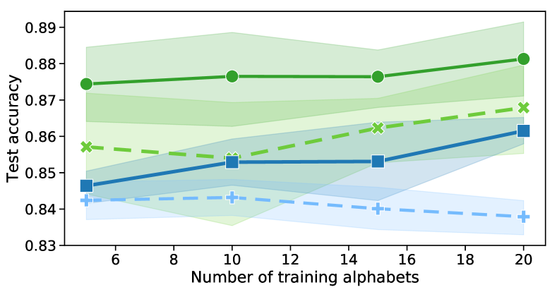
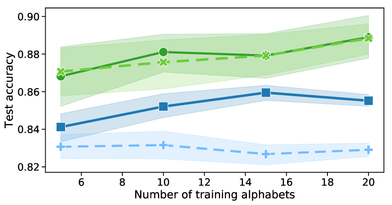
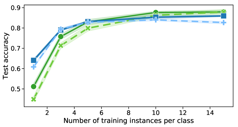
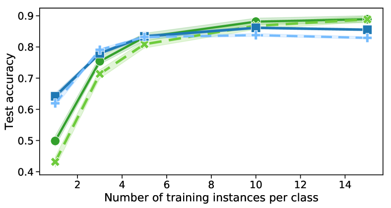
In the small-data regime, we evaluate the performance of Reptile, iMAML, $\boldsymbol{\sigma}$-Reptile, and $\boldsymbol{\sigma}$-iMAML across variants of the many-shot augmented Omniglot task with different numbers of training alphabets and training image instances per character class, without rotation augmentation. We train each algorithm $10$ times with each of $5,10,15,$ and $20$ training alphabets and $1,3,5,10,$ and $15$ training instances per character class.

We meta-train all algorithms for $1000$ steps using $100$ steps of adaptation per task. We use a meta-batch size of $20$, meaning that the same task can appear multiple times within a batch, although the images will be different in each task instance due to data augmentation. At meta-evaluation time, we again perform $100$ steps of task adaptation on the task-train instances of each test alphabet, and report the accuracy on the task-validation instances.

Hyperparameters for each of the $4$ algorithms that we evaluate on small-data augmented Omniglot are listed in Table 5. These were chosen based on a comprehensive hyperparameter search on separate validation data. For Reptile, we use a linear learning rate decay that reaches $0$ at the end of meta-training, as in Nichol et al. [2]. For iMAML, we use an L2 regularization scale of $\lambda=1/\sigma^{2}=1$e$-3$. For $\boldsymbol{\sigma}$-iMAML and $\boldsymbol{\sigma}$-Reptile, we use a different task optimizer learning rate for different numbers of instances. These learning rates are presented in Table 6.

Due to the space limit, we show results with 1 training instance per character class and results with 15 training alphabets in Fig. 4 of the main text. The full results of the $20$ experimental conditions are presented in Figs. 10 and 11, which respectively show the performance of each method as the number of training instances and alphabets vary. As discussed in the main text, each shrinkage variant outperforms or matches its corresponding non-shrinkage variant in nearly every condition. Improvements by the shrinkage variants are more consistent and pronounced when the amount of training data is limited.

E.2 Few-shot Text-to-Speech experiment details

Figure 12: Architecture of the multi-speaker WaveNet model. The single-speaker WaveNet model used by Reptile and $\boldsymbol{\sigma}$-Reptile, does not include the speaker embedding lookup table and the corresponding conditional input layer.

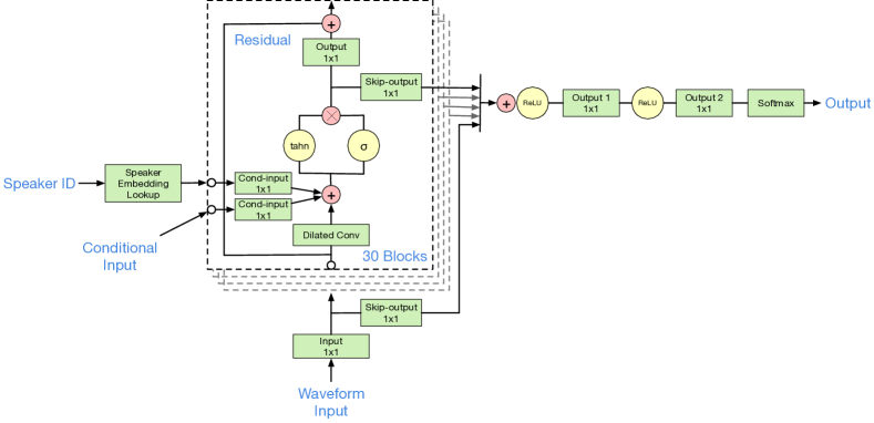
For few-shot text-to-speech synthesis, various works [6, 1, 7, 8] have made use of speaker-encoding networks or trainable speaker embedding vectors to adapt to a new voice based on a small amount of speech data. These works achieved success to some extent when there were a few training utterances, but the performance saturated quickly beyond 10 utterances [7] due to the bottleneck in the speaker specific components. Arik et al. [6] and Chen et al. [1] found that the performance kept improving with more utterances by fine-tuning the entire TTS model, but the adaptation process had to be terminated early to prevent overfitting. As such, some modules may still be underfit while others have begun to overfit, similar to the behavior seen for MAML in Fig. 8.

In this paper, we examine the advantages of shrinkage for a WaveNet model [21]. The same method applies to other TTS architectures as well. In preliminary experiments, we found iMAML and $\boldsymbol{\sigma}$-iMAML meta-learn much more slowly than Reptile and $\boldsymbol{\sigma}$-Reptile. We conjecture that this is because iMAML and $\boldsymbol{\sigma}$-iMAML compute meta-gradients based only on the validation data from the last mini-batch of task adaptation. In contrast, the meta update for $\boldsymbol{\phi}$ from Reptile and $\boldsymbol{\sigma}$-Reptile accumulates the task parameter updates computed from training mini-batches through the adaptation process. With a task adaptation horizon of 100 steps, this leads to significantly different data efficiencies. As a result, we only evaluate Reptile and $\boldsymbol{\sigma}$-Reptile for this experiment.

The WaveNet model is an augoregressive generative model. At every step, it takes the sequence of waveform samples generated up to that step, and the concatenated fundamental frequency (f0) and linguistic feature sequences as inputs, and predicts the sample at the next step. The sequence of fundamental frequency controls the dynamics of the pitch in an utterance. The short-time frequency is important for WaveNet to predict low level sinusoid-like waveform features. The linguistic features encode the sequence of phonemes from text. They are used by WaveNet to generate speech with corresponding content. The dynamics of the fundamental frequency in f0 together with the phoneme duration contained in the linguistic feature sequence contains important information about the prosody of an utterance (word speed, pauses, emphasis, emotion, etc), which change at a much slower time-scale. While the fundamental frequency and prosody in the inputs contain some information about the speaker identity, the vocal tract characteristics of a voice that is unique to each speaker cannot be inferred from the inputs, and has to be learned by the WaveNet model from waveform samples through task adaptation.

The full architecture of a multi-speaker WaveNet model used by SEA-Emb and SEA-All in Chen et al. [1] is shown in Fig. 12. For Reptile and $\boldsymbol{\sigma}$-Reptile, we use a single-speaker model architecture that excludes the speaker embedding lookup table and associated conditional input layers in the residual blocks. The single-speaker model is comprised of one input convolutional layer with $1\times 1$ kernel, one input skip-output $1\times 1$ layer, 30 residual of dilated causal-convolutional blocks (each including 4 layers), and 2 $1\times 1$ output layers before feeding into a 256-way softmax layer. We treat every layer as a module, for a total of 123 modules (the output layer of the last block is not used for prediction).

To speed up meta-learning, we first pretrain a single-speaker model with all training speaker data mixed, and initialize $\boldsymbol{\sigma}$-Reptile and Reptile with that pretrained model. This is reminiscent of other meta-learning works for few-shot image classification that use a pretrained multi-head model to warm-start when the backbone model (e.g. ResNet) is large. This pretrained TTS model learns to generate speech-like samples but does not maintain a consistent voice through a single sentence In contrast to other meta-learning works that fix the feature extracting layers, we then meta-learn all WaveNet layers to identify most task-specific modules.

We run the multispeaker training and pre-training for meta-learning methods for 1M steps on a proprietary dataset of 61 speakers each with 2 hours of speech data with 8-bit encoding sampled at 24K frequency. For $\boldsymbol{\sigma}$-Reptile and Reptile, we further run meta-learning for 8K meta-steps with 100 task adaptation steps in the inner loop for the same set of speakers. Each task consists of 100 utterances (roughly 8 minutes of speech). We evaluate the model on 10 holdout speakers, in two data settings, with 100 utterances or 50 utterances (roughly 4 minutes of speech) per task. We run up to 10,000 task adaptation steps in meta-test. SEA-All and Reptile both finetune all parameters. They overfit quickly in meta-testing after about 1,500 and 3,000 adaptation steps with 4-min and 8-min of data, respectively. We therefore early terminate task adaptation for these algorithms to prevent overfitting.

To measure the sample quality of naturalness, we have human evaluators rate each sample on a five-point Likert Scale (1: Bad, 2: Poor, 3: Fair, 4: Good, 5: Excellent) and then we compute the mean opinion score (MOS). This is the standard approach to evaluate the quality of TTS models.

Voice similarity is computed as follows. We use a pretrained speaker verification model [47] that outputs an embedding vector, $d(x)$, known as a $d$-vector, for each utterance $x$. We first compute the mean of $d$-vectors from real utterances of each test speaker, $t$. $\bar{d}_{t}:=\sum_{n}d(x_{t,n})/N_{t}$. Given a model adapted to speaker $t$, we compute the sample similarity for every sample utterance $x_{i}$ as

$$\mathrm{sim}(x_{i},t)=\mathrm{cos}(d(x_{i}),\bar{d}_{t})\,.$$

E.3 Additional short adaptation experiment: sinusoid regression

We follow the standard sinusoid regression protocol of Finn et al. [13] in which each task consists of regressing input to output of a sinusoid $y=a\sin(x-b)$ uniformly sampled with amplitude $a\in[0.1,5]$ and phase $b\in[0,\pi]$. Each task is constructed by sampling $10$ labelled data points from input range $x\in[-5,5]$. We learn a regression function with a 2-layer neural network with 40 hidden units and ReLU nonlinearities and optimise the mean-squared error (MSE) between predictions and true output values.

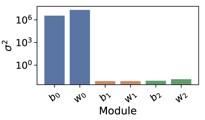
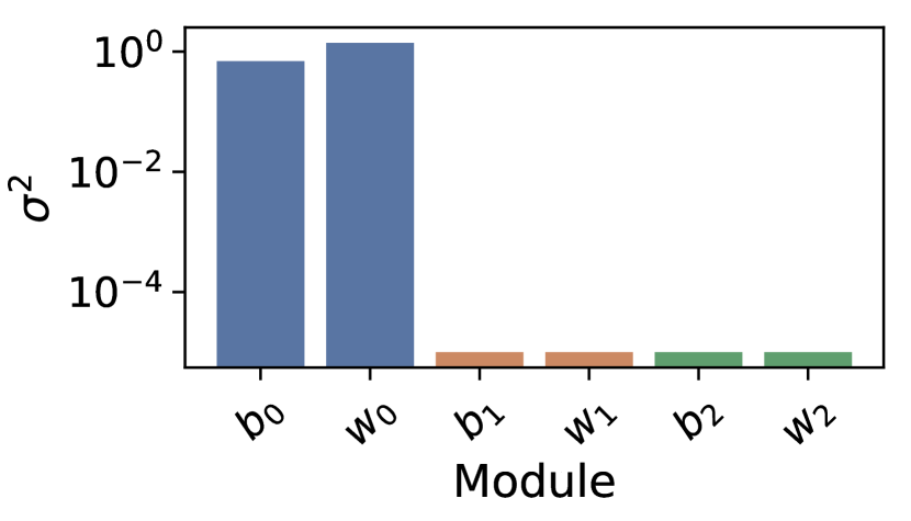
Our method is agnostic to the choice of modules. For this small model, consider each set of network parameters as a separate module. In total, we define 6 modules: $\{b_{i},w_{i}\}$, for $i=0,1,2$, where $b_{i}$ and $w_{i}$ denote the bias and weights of each layer. We run each shrinkage variant for 100K meta-training steps, and evaluate the generalization error on 100 holdout tasks. The hyperparameters of all three shrinkage algorithm variants are given in Table 7.

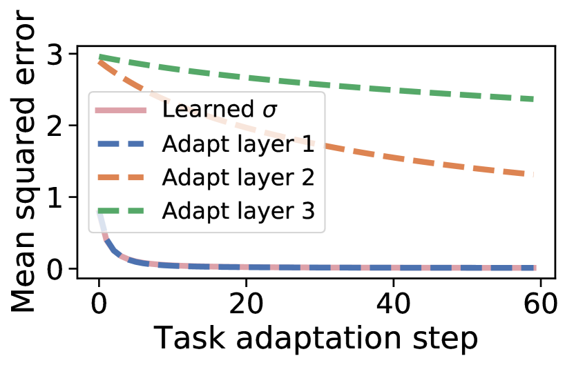
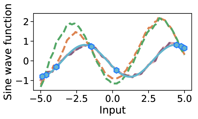
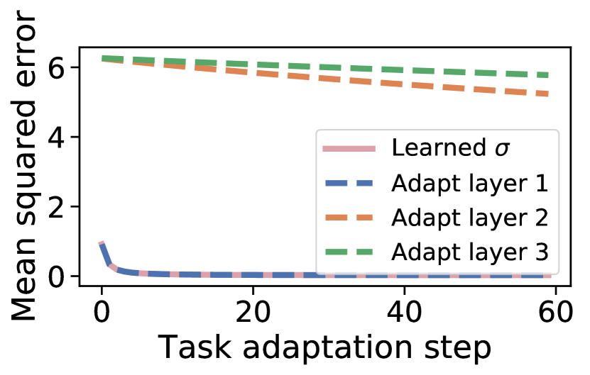
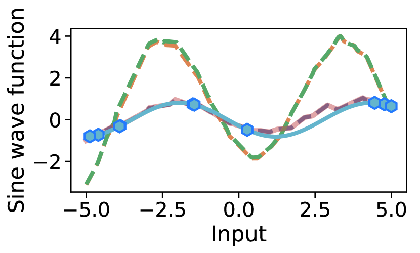
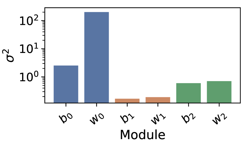
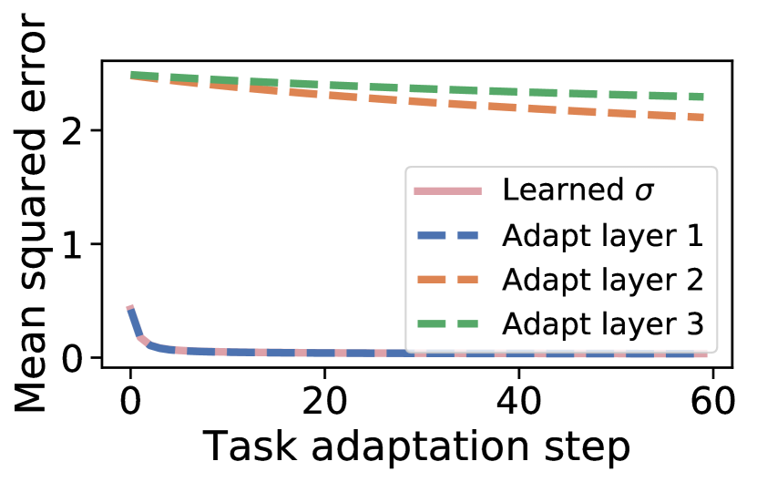
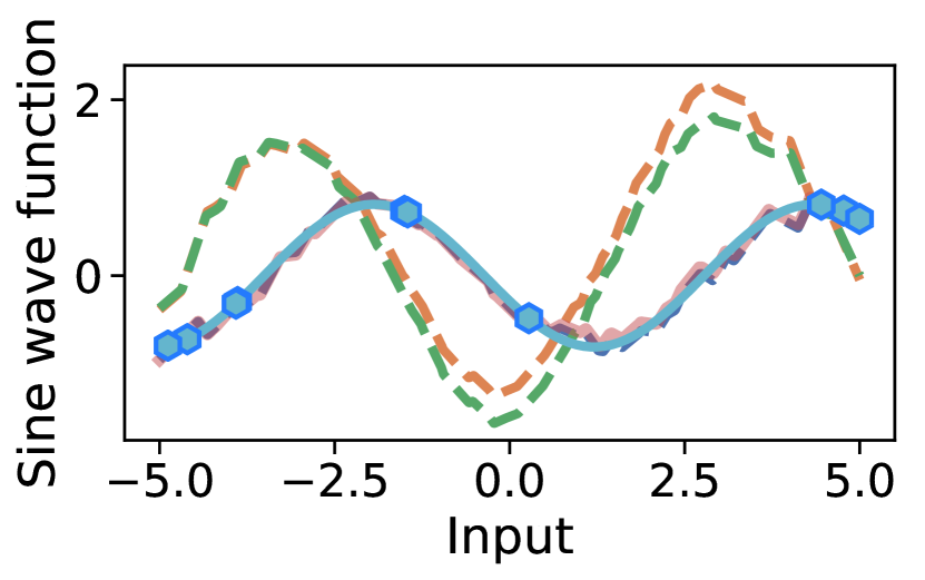
We show the learned variance from $\boldsymbol{\sigma}$-MAML, $\boldsymbol{\sigma}$-iMAML and $\boldsymbol{\sigma}$-Reptile in Fig. 13(13(a),13(d),13(g)) respectively. In all experiments, we observe that the learned variances $\sigma_{m}^{2}$ for the first 2 modules ($b_{0},w_{0}$) are significantly larger than the rest. This implies that our method discovers that these modules are task-specific and should change during adaptation whereas the other modules are task-independent.

To confirm that the learned variances correspond to task-specificity, we adapt one layer at a time on holdout tasks and keep the other layers fixed. Fig. 13 shows that adapting only the discovered first layer results in both low error and accurately reconstructed sinusoids, whereas adapting the other modules does not.

Table 7: Hyperparameters for the few-shot sinusoid regression experiment. Chosen with random search on validation task set.

	$\boldsymbol{\sigma}$-MAML	$\boldsymbol{\sigma}$-Reptile	$\boldsymbol{\sigma}$-iMAML
Meta-training
Meta optimizer	Adam	Adam	Adam
Meta learning rate ($\boldsymbol{\phi}$)	9.8e-4	3.0e-3	5.7e-3
Meta learning rate ($\log\boldsymbol{\sigma}^{2}$)	4.4e-3	1.4e-4	1.8e-3
Meta training steps	100k	100k	100k
Meta batch size (# tasks)	5	5	5
Damping coefficient	-	6e-3	0.5
Conjugate gradient steps	-	7	1
Task adaptation
Task optimizer	ProximalGD	ProximalGD	ProximalGD
Task learning rate	8.3e-4	1.4e-4	3.9e-4
Task adaptation steps	68	100	100
Task batch size (# data points)	10	10	10

(a) Learned $\boldsymbol{\sigma}$ for each module ($\boldsymbol{\sigma}$-MAML).

(b) MSE under different adaptation schemes.

(c) Prediction after 60 steps of adaptation.

(d) Learned $\boldsymbol{\sigma}$ for each module ($\boldsymbol{\sigma}$-iMAML).

(e) MSE under different adaptation schemes.

(f) Prediction after 60 steps of adaptation.

(g) Learned $\sigma$ for each module ($\boldsymbol{\sigma}$-Reptile).

(h) MSE under different adaptation schemes.

(i) Prediction after 60 steps of adaptation.

Figure 13: Sinusoid regression with $\boldsymbol{\sigma}$-MAML (top row), $\boldsymbol{\sigma}$-iMAML (middle row), and $\boldsymbol{\sigma}$-Reptile (bottom row). In the left column (13(a),13(d),13(g)) we show the learned $\sigma_{m}$ for each module. In the middle column (13(b),13(e),13(h)) we show the mean squared error, averaged over 100 tasks, as a function of task adaptation step, while adapting only a single module (the dashed lines) or using the learned $\boldsymbol{\sigma}$ (pink). Finally, the right column (13(c),13(f),13(i)) shows predictions under each adaptation scheme. Note that the model trained using the learned $\boldsymbol{\sigma}$ (pink) overlaps with the model with the first layer adapted (dark blue) in (13(b)–13(c),13(e)–13(f),13(h)–13(i)).

E.4 Additional short adaptation experiment: few-shot image classification

We next look at two standard benchmarks for few-shot image classification, Omniglot and miniImageNet, which perform task adaptation in meta-training for up to 20 steps.

E.4.1 Few-shot Omniglot

The Omniglot dataset [48, 49] consists of 20 samples of 1623 characters from 50 different alphabets. The dataset is augmented by creating new characters that are rotations of each of the existing characters by $0,90,180,$ or $270$ degrees. We follow the standard $N$-way $K$-shot classification setting where a task is generated by randomly sampling $N$ characters and training the model on $K$ instances of each  [49, 50, 51]. Character classes are partitioned into separate meta-train and meta-test splits, and the instances (images) of each character are also split into separate (task) train and (task) validation subsets.

We use the same $4$-block convolutional architecture as in Finn et al. [13]. This architecture consists of $4$ convolutional blocks, each made up of a $3\times 3$ convolutional layer with $64$ filters and stride $2$, a batch-normalization layer [52], and a ReLU activation, in that order. The output of the final convolutional block is fed into an output linear layer and a softmax, and trained with the cross-entropy loss. All images are downsampled to $28\times 28$.

Hyperparameters for the six algorithms evaluated in this experiment are presented in Table 8. Module discovery and classification performance for this dataset are discussed below.

Table 8: Hyperparameters for the few-shot Omniglot classification. Chosen with random search on the validation task set.

	MAML	Reptile	iMAML	$\boldsymbol{\sigma}$-MAML	$\boldsymbol{\sigma}$-Reptile	$\boldsymbol{\sigma}$-iMAML
Meta-training
Meta optimizer	Adam	SGD	Adam	Adam	SGD	Adam
Meta learning rate ($\boldsymbol{\phi}$)	4.8e-3	1.8	1e-3	1.7e-4	1.6	7.8e-3
Meta learning rate ($\log\boldsymbol{\sigma}^{2}$)	-	-	-	7.4e-3	7e-4	4e-3
Meta training steps	60k	100k	60k	60k	100k	60K
Meta batch size (# tasks)	32	5	32	32	5	32
Damping coefficient	-	-	1.0	-	6e-3	0.18,
Conjugate gradient steps	-	-	4	-	1	2
Task adaptation (adaptation step and batch size for meta-test are in parentheses)
Task optimizer	SGD	Adam	ProximalGD	ProximalGD	Adam	ProximalGD
Task learning rate	0.968	8e-4	0.23	0.9	6e-4	1.3
Task adaptation steps	1 (50)	5 (50)	19 (50)	3 (50)	8 (50)	8 (50)
Task batch size (# images)	5 (5)	10 (5)	5 (5)	5 (5)	10 (5)	5 (5)

E.4.2 miniImageNet

The miniImageNet dataset [50, 51] is, as the name implies, a smaller and easier many-task, few-shot variant of the ImageNet dataset. However, its images are larger and more challenging than those of Omniglot. miniImageNet consists of $100$ classes ($64$ train, $12$ validation, and $24$ test) with images downsampled to $84\times 84$. We follow the standard miniImageNet protocol and train in the $N$-way $K$-shot paradigm using the same $4$-block convolutional architecture as in previous work [50, 13]. Each convolutional block consists of a $3\times 3$ convolutional layer with $32$ filters, a batch-normalization layer [52], and a ReLU activation, in that order. As in Omniglot, the output of the final convolutional block is fed into an output linear layer and a softmax, and trained with the cross-entropy loss.

Hyperparameters for each algorithm on miniImageNet are presented in Table 9. For iMAML, we use $\lambda=0.14$. Module discovery and classification performance for this dataset are discussed below.

Table 9: Hyperparameters for the few-shot miniImageNet classification experiment. Chosen with random search on validation task set.

	MAML	Reptile	iMAML	$\boldsymbol{\sigma}$-MAML	$\boldsymbol{\sigma}$-Reptile	$\boldsymbol{\sigma}$-iMAML
Meta-training
Meta optimizer	Adam	SGD	Adam	Adam	Adam	Adam
Meta learning rate ($\boldsymbol{\phi}$)	1e-3	0.45	2.5e-4	1e-3	6e-4	2e-4
Meta learning rate ($\log\boldsymbol{\sigma}^{2}$)	-	-	-	5e-2	2.5e-2	0.2
Meta training steps	60k	100k	60k	60k	100k	60k
Meta batch size (# tasks)	4	5	4	5	3	5
Damping coefficient	-	-	6.5e-2	-	1e-2	2e-3
Conjugate gradient steps	-	-	5	-	3	2
Task adaptation (adaptation step and batch size for meta-test are in parentheses)
Task optimizer	SGD	Adam	ProximalGD	ProximalGD	ProximalGD	ProximalGD
Task learning rate	1e-2	1.5e-3	4e-2	0.1	1.35	1.6
Task adaptation steps	5 (50)	5 (50)	17 (50)	5 (50)	7 (50)	1 (50)
Task batch size (# images)	5 (5)	10 (5)	5 (5)	5 (5)	10 (5)	5 (5)

(a) Learned $\sigma^{2}$ for $\boldsymbol{\sigma}$-MAML.

(b) Learned $\sigma^{2}$, $\boldsymbol{\sigma}$-iMAML.

(c) Learned $\sigma^{2}$ for $\boldsymbol{\sigma}$-Reptile.

(d) Accuracy for $\boldsymbol{\sigma}$-MAML.

(e) Accuracy, $\boldsymbol{\sigma}$-iMAML.

(f) Accuracy for $\boldsymbol{\sigma}$-Reptile.

Figure 14: Learned variances and test accuracies on Omniglot. (a) & (b) & (c) show the learned variance per module with $\boldsymbol{\sigma}$-MAML, $\boldsymbol{\sigma}$-iMAML and $\boldsymbol{\sigma}$-Reptile, respectively. (d) & (e) & (f) show the average test accuracy at the end of task adaptation with $\boldsymbol{\sigma}$-MAML, $\boldsymbol{\sigma}$-iMAML and $\boldsymbol{\sigma}$-Reptile. Each bar shows the accuracy after task adaptation either with all layers frozen except one. Colors map to the colors of (a) & (b) & (c). $\mathrm{bn}_{i}$ and $\mathrm{conv}_{i}$ denote $i$-th batch normalization layer and convolutional layer, and $\mathrm{output}$ is the linear output layer. The pink dashed line shows the accuracy after adaptation with the learned $\sigma$ and the black dashed line is the chance accuracy.

(a) Learned $\sigma^{2}$ for $\boldsymbol{\sigma}$-MAML.

(b) Learned $\sigma^{2}$, $\boldsymbol{\sigma}$-iMAML.

(c) Learned $\sigma^{2}$ for $\boldsymbol{\sigma}$-Reptile.

(d) Accuracy for $\boldsymbol{\sigma}$-MAML.

(e) Accuracy, $\boldsymbol{\sigma}$-iMAML.

(f) Accuracy for $\boldsymbol{\sigma}$-Reptile.

Figure 15: Learned variances and test accuracies on miniImageNet. (a) & (b) & (c) show the learned variance per module with $\boldsymbol{\sigma}$-MAML, $\boldsymbol{\sigma}$-iMAML and $\boldsymbol{\sigma}$-Reptile, respectively. (d) & (e) & (f) show the average test accuracy during at the end of task adaptation with $\boldsymbol{\sigma}$-MAML, $\boldsymbol{\sigma}$-iMAML and $\boldsymbol{\sigma}$-Reptile. Each bar shows the accuracy after task adaptation either with all layers frozen except one. Colors map to the colors of (a) & (b) & (c). $\mathrm{bn}_{i}$ and $\mathrm{conv}_{i}$ denote $i$-th batch normalization layer and convolutional layer, and $\mathrm{output}$ is the linear output layer. The pink dashed line shows the accuracy after adaptation with the learned $\sigma$ and the black dashed line is the chance accuracy.

Figure 16: Learned variances of the last conv layer vs output linear layer with $\boldsymbol{\sigma}$-iMAML from multiple runs.

Table 10: Test accuracy on few-shot Omniglot and few-shot miniImageNet. For each algorithm, we report the mean and $95\%$ confidence interval over $10$ different runs. For each pair of corresponding methods, we bold the entry if there exists a statistically significant difference.

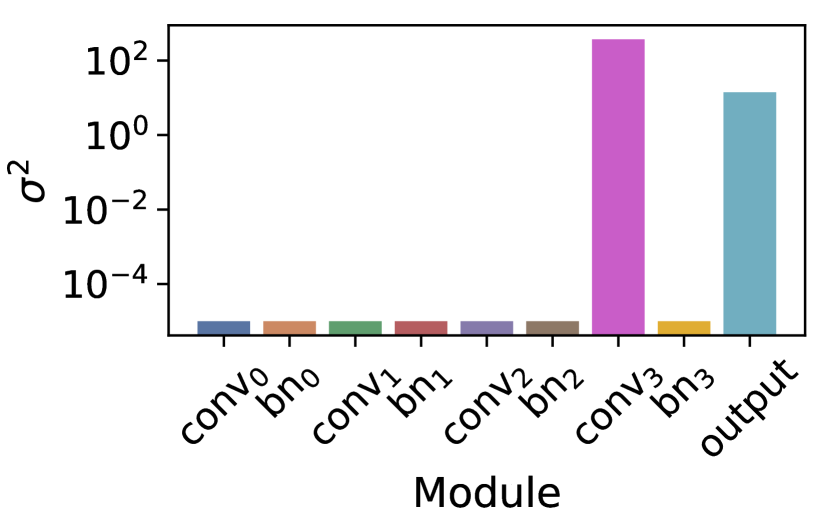
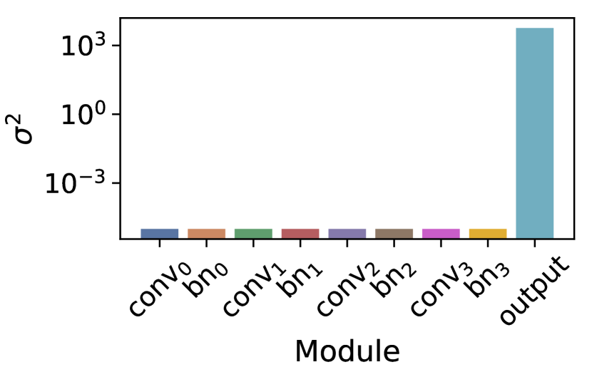
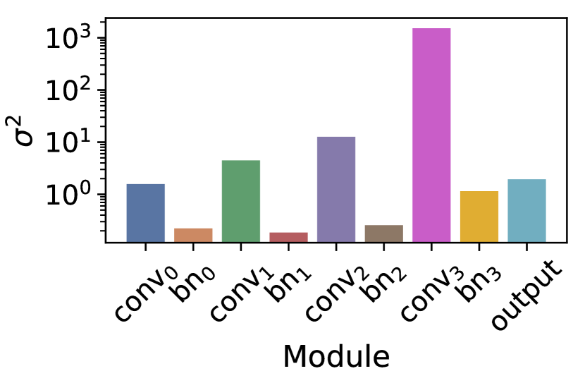
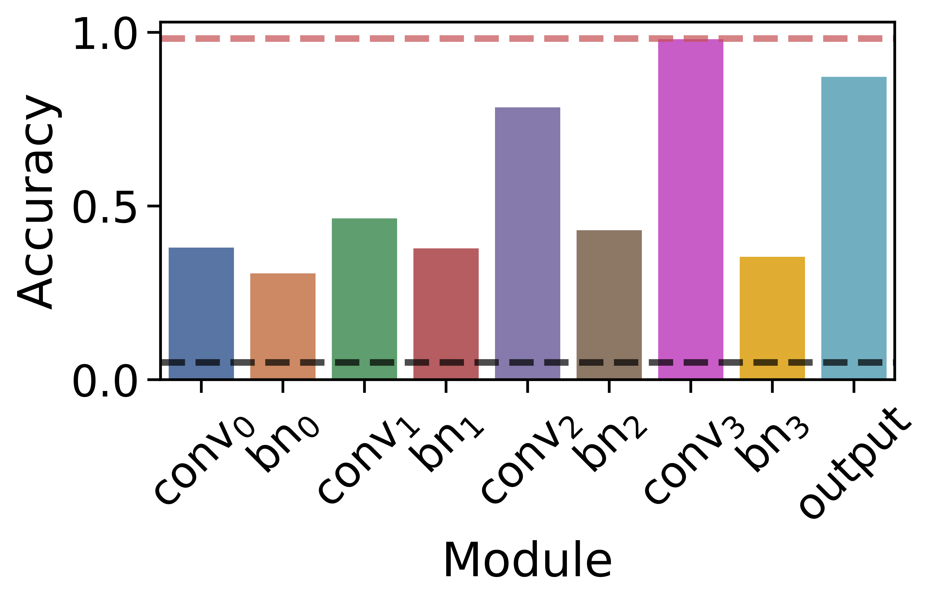
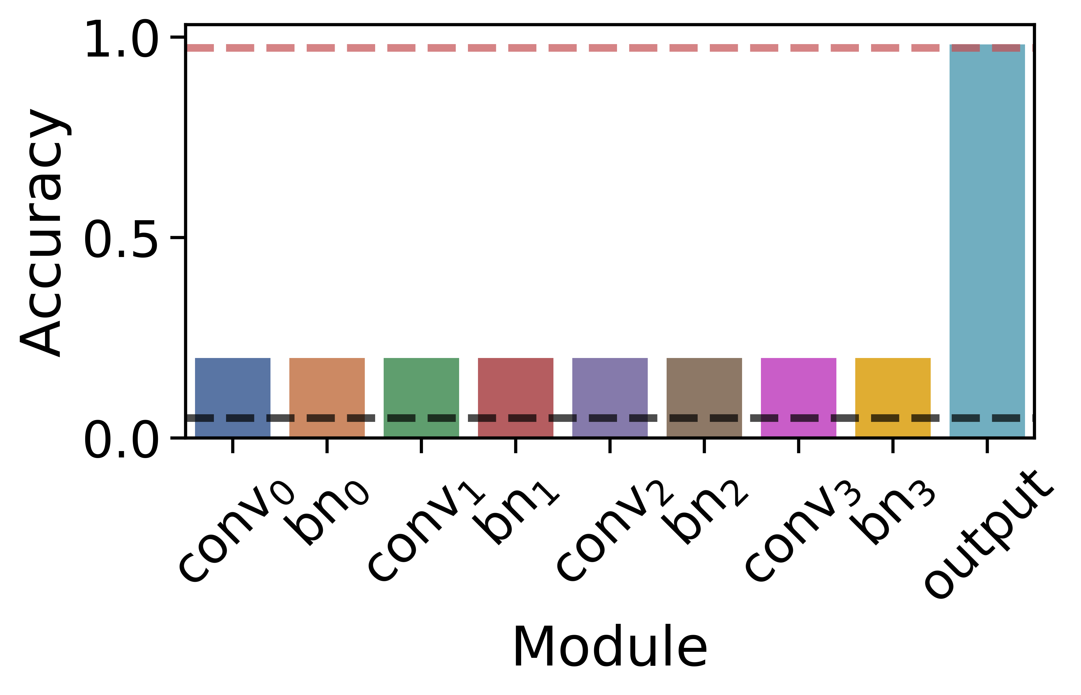
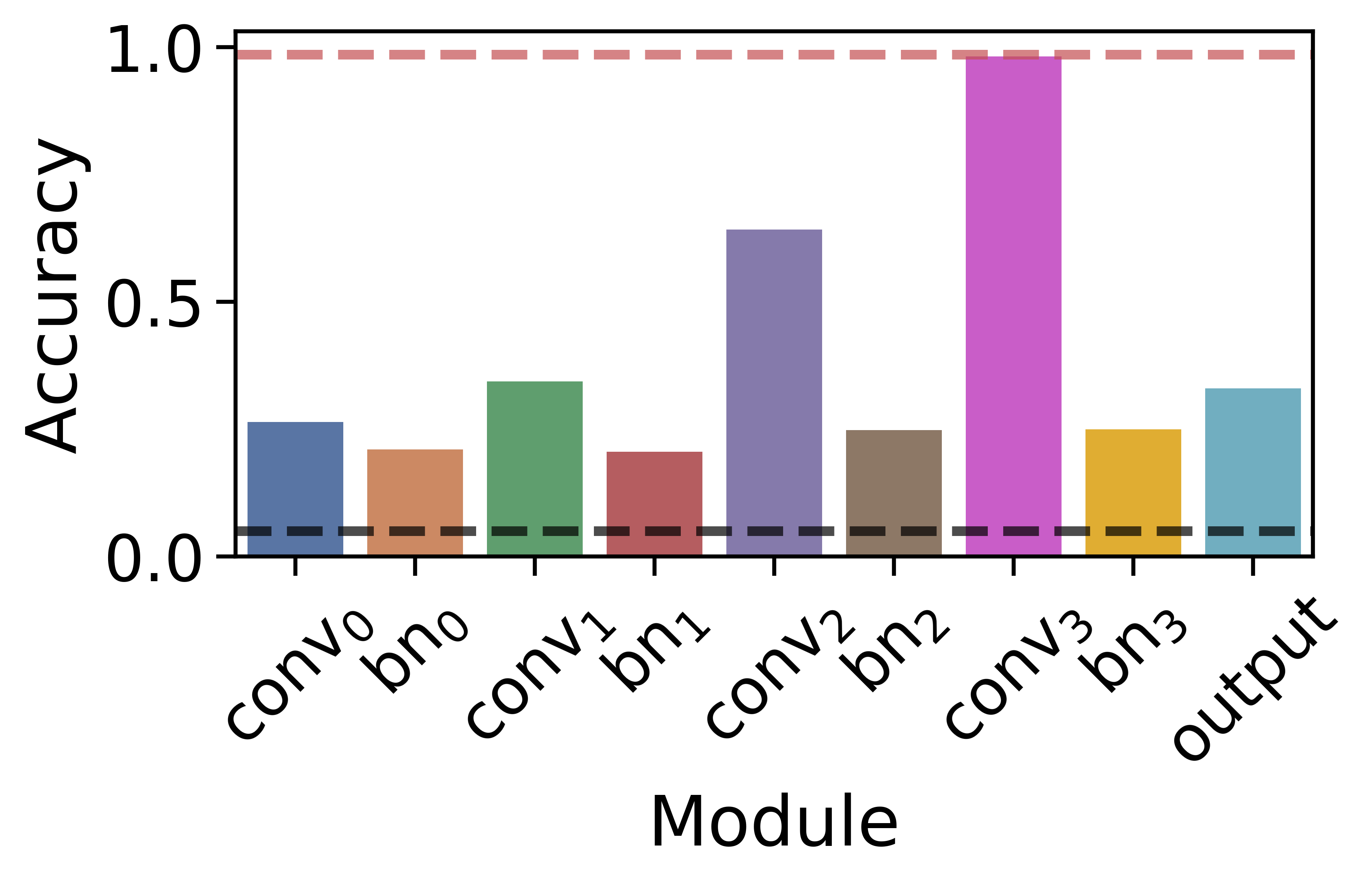
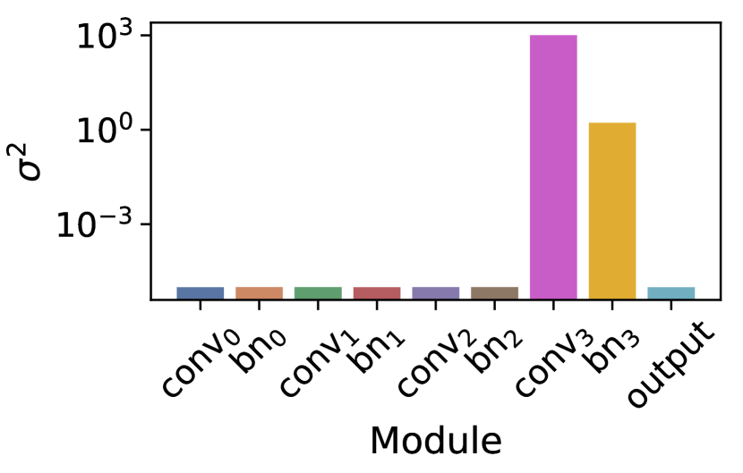
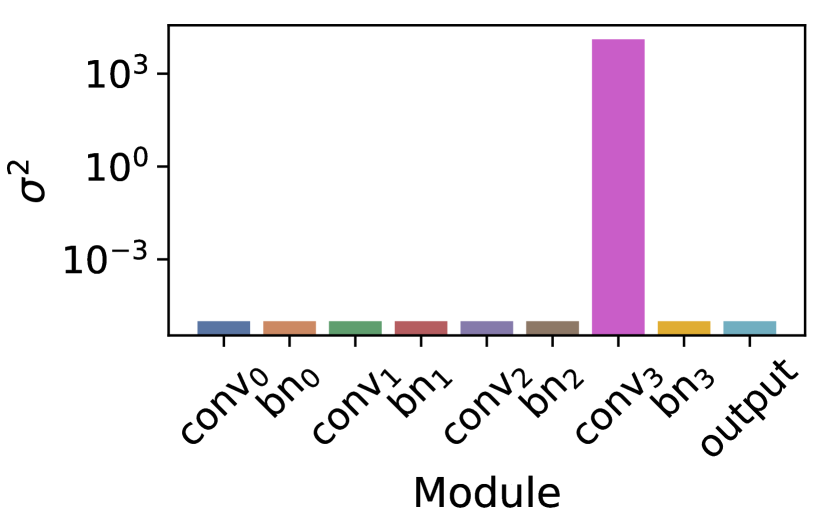
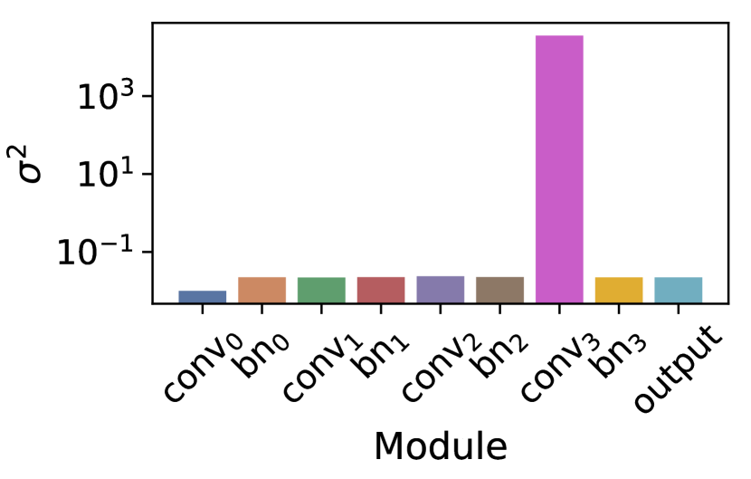
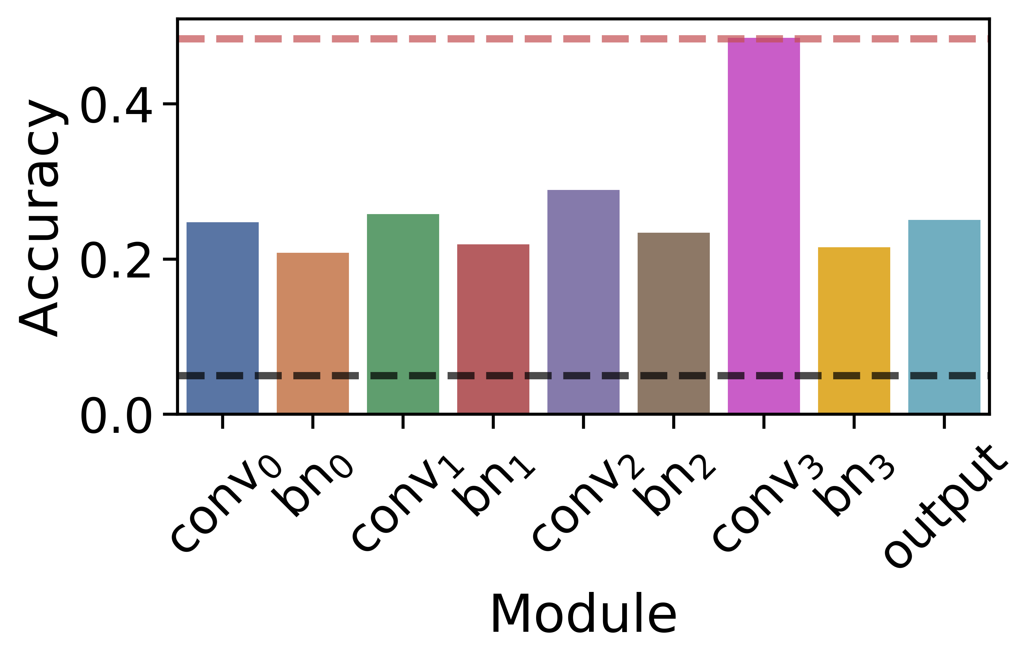
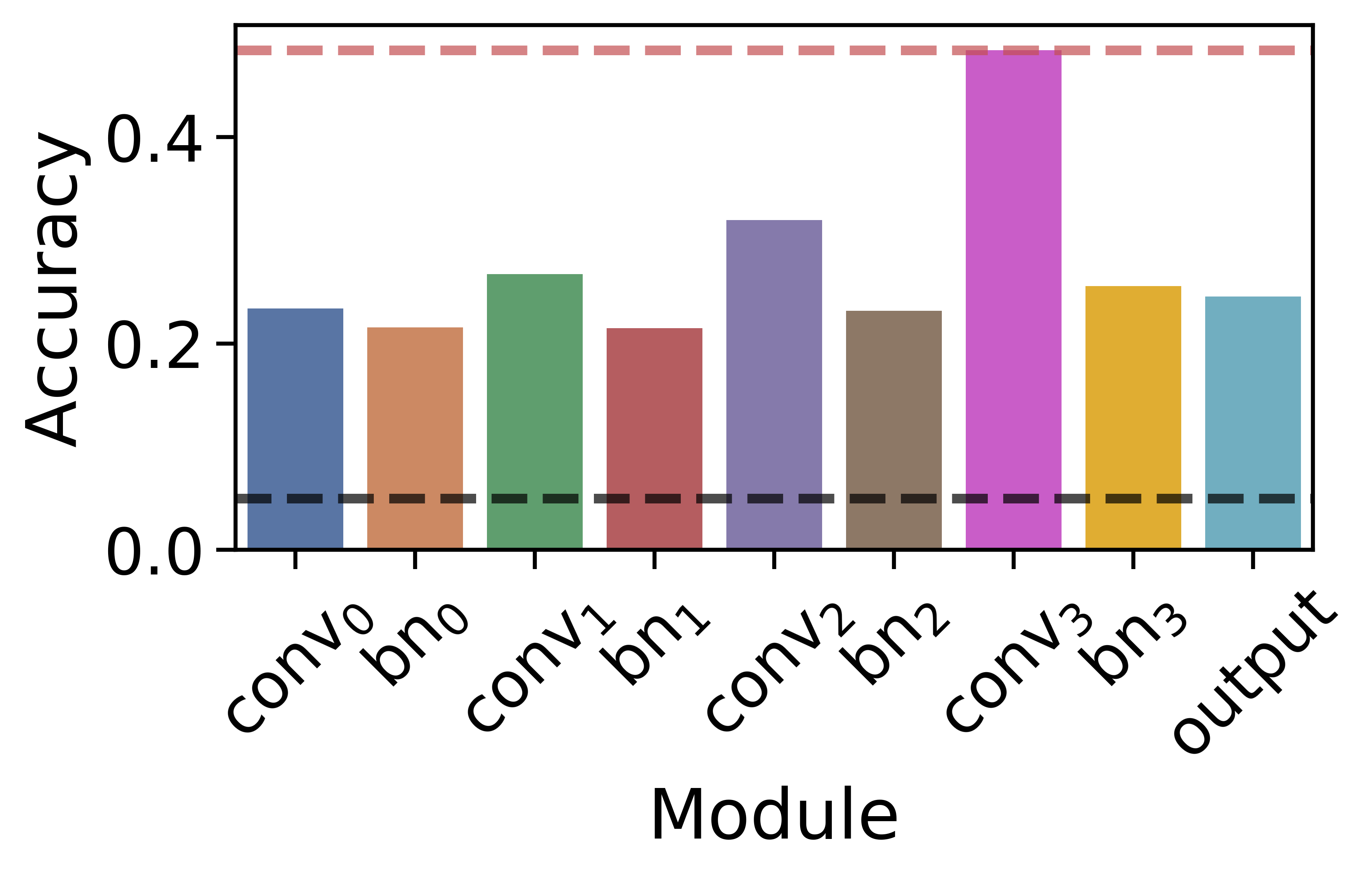
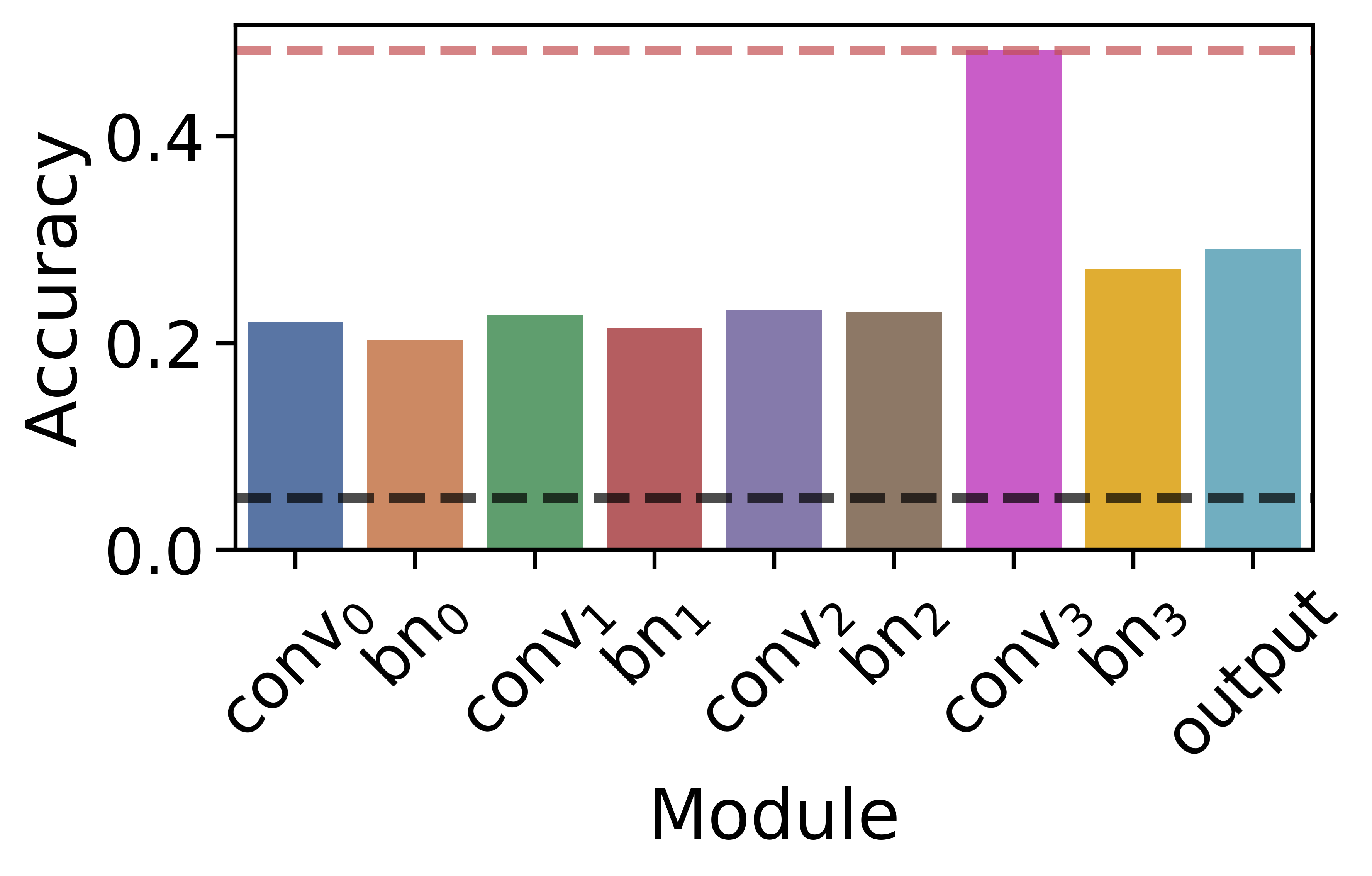
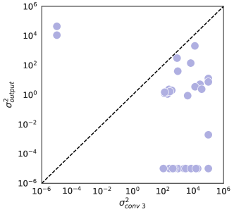
	Omniglot	miniImageNet
	$N5$ $K1$	$N5$ $K1$
$\boldsymbol{\sigma}$-MAML	$98.8\pm 0.4\%$	$\mathbf{47.7\pm 0.5\%}$
MAML	$98.7\pm 0.7\%$	$46.1\pm 0.8\%$
$\boldsymbol{\sigma}$-iMAML	$97.2\pm 0.8\%$	$47.6\pm 1.1\%$
iMAML	$97.2\pm 1.2\%$	$47.2\pm 1.4\%$
$\boldsymbol{\sigma}$-Reptile	$\mathbf{97.8\pm 0.5\%}$	$47.0\pm 0.9\%$
Reptile	$96.9\pm 0.6\%$	$47.4\pm 0.9\%$

E.4.3 Module discovery

We first discuss module discovery for these two datasets and then compare classification accuracies in the next section.

Fig. 14 and Fig. 15 present our module discovery results for all three shrinkage algorithms on few-shot Omniglot and miniImageNet. We see that after training there is always one layer that has a learned variance that is much larger than all other layers. As shown in Fig. 14(d-e) and Fig. 15(d-e), we observe that by adapting only this task-specific module, the model is able to achieve high accuracy at test time, equal to the performance achieved when adapting all layers according to the learned $\boldsymbol{\sigma}^{2}$. Conversely, adapting only the task-independent modules leads to poor performance.

Importantly, it is always one of the final two output layers that has the highest learned variance, meaning that these two layers are the most task-specific. This corroborates the conventional belief in image-classification convnets that output layers are more task-specific while input layers are more general, which is also validated in other meta-learning works [17, 25].

However, in most of the subfigures in Fig. 14 and Fig. 15, it is actually the penultimate layer that is most task-specific and should be adapted. The only algorithm for which the penultimate layer was not the most task-specific was $\boldsymbol{\sigma}$-iMAML in the Omniglot experiment. To study this further, we run $\boldsymbol{\sigma}$-iMAML on Omniglot repeatedly with a random initialization and hyper-parameter settings and keep the learned models that achieve at least $95\%$ test accuracy. In Fig. 16, we show the learned $\sigma_{m}^{2}$ of the final convolutional layer ($conv_{3}$) and the linear output layer ($output$) from those runs. In almost every case, $conv_{3}$ dominates $output$ by an order of magnitude, meaning that the selection of the output layer in Fig. 14 was a rare event due to randomness. Adapting $conv_{3}$ remains the most stable choice, and most runs that adapt only it achieve a test accuracy that is not statistically significantly different from the result in Fig. 14(b). Our results extend the results of the above meta-learning works that focus only on adapting the final output layer, and match a recent independent observation in Arnold et al. [19].

Considering the different task-specific modules discovered in augmented Omniglot, TTS, sinusoid regression, and these two short-adaptation datasets, it is clearly quite challenging to hand-select task-specific modules a priori. Instead, meta-learning a shrinkage prior provides a flexible and general method for identifying the task-specific and task-independent modules for the domain at hand.

Learning a prior for a single module.
We also tried learning a single shared prior $\sigma^{2}$ for all variables. When using a single module like this, $\sigma^{2}$ grows steadily larger during meta-learning, and the shrinkage algorithms simply reduce to their corresponding standard meta-learning algorithms without the shrinkage prior. This highlights the necessity of learning different priors for different components of a model.

This observation differs from the results of Rajeswaran et al. [3], which reported an optimal value of $\lambda=1/\sigma^{2}=2$ for iMAML. One possible explanation for this difference is that too small of a value for $\lambda$ leads to instability in computing the implicit gradient, which hinders learning. Also, when searching for the optimal $\lambda$ as a hyperparameter the dependence of the validation loss on $\lambda$ becomes less clear when $\lambda$ is sufficiently small. In our few-shot Omniglot experiments, we find that the best value of $\lambda$ for iMAML is $\lambda=0.025$.

E.4.4 Classification accuracy

We compare the predictive performance of all methods on held-out tasks in Table 10. While many of the results are not statistically different, the shrinkage variants show a modest but consistent improvement over the non-shrinkage algorithms. Further, $\boldsymbol{\sigma}$-MAML does significantly outperform MAML on miniImageNet and $\boldsymbol{\sigma}$-Reptile does significantly outperform Reptile in Omniglot.

Note that we do not in general expect the shrinkage variants to significantly outperform their counterparts here because the latter do not exhibit overfitting issues on these datasets and have comparable or better accuracy than other Bayesian methods in the literature [26, 22].

References

- Chen et al. [2019] Yutian Chen, Yannis Assael, Brendan Shillingford, David Budden, Scott Reed, Heiga Zen, Quan Wang, Luis C. Cobo, Andrew Trask, Ben Laurie, Caglar Gulcehre, Aaron van den Oord, Oriol Vinyals, and Nando de Freitas. Sample efficient adaptive text-to-speech. In International Conference on Learning Representations, 2019.
- Nichol et al. [2018] Alex Nichol, Joshua Achiam, and John Schulman. On first-order meta-learning algorithms. arXiv preprint arXiv:1803.02999, 2018.
- Rajeswaran et al. [2019] Aravind Rajeswaran, Chelsea Finn, Sham M Kakade, and Sergey Levine. Meta-learning with implicit gradients. In Advances in Neural Information Processing Systems, pages 113–124, 2019.
- Flennerhag et al. [2019a] Sebastian Flennerhag, Pablo G. Moreno, Neil D. Lawrence, and Andreas Damianou. Transferring knowledge across learning processes. In International Conference on Learning Representations, 2019a.
- Flennerhag et al. [2019b] Sebastian Flennerhag, Andrei A Rusu, Razvan Pascanu, Francesco Visin, Hujun Yin, and Raia Hadsell. Meta-learning with warped gradient descent. In International Conference on Learning Representations, 2019b.
- Arik et al. [2018] Sercan Arik, Jitong Chen, Kainan Peng, Wei Ping, and Yanqi Zhou. Neural voice cloning with a few samples. In Advances in Neural Information Processing Systems, pages 10019–10029, 2018.
- Jia et al. [2018] Ye Jia, Yu Zhang, Ron Weiss, Quan Wang, Jonathan Shen, Fei Ren, Patrick Nguyen, Ruoming Pang, Ignacio Lopez Moreno, and Yonghui Wu. Transfer learning from speaker verification to multispeaker text-to-speech synthesis. In Advances in Neural Information Processing Systems, pages 4480–4490, 2018.
- Taigman et al. [2018] Yaniv Taigman, Lior Wolf, Adam Polyak, and Eliya Nachmani. Voiceloop: Voice fitting and synthesis via a phonological loop. In International Conference on Learning Representations, 2018.
- Peters et al. [2017] Jonas Peters, Dominik Janzing, and Bernhard Schölkopf. Elements of Causal Inference: Foundations and Learning Algorithms. MIT Press, 2017.
- Parascandolo et al. [2018] Giambattista Parascandolo, Niki Kilbertus, Mateo Rojas-Carulla, and Bernhard Schölkopf. Learning independent causal mechanisms. In International Conference on Machine Learning, pages 4036–4044, 2018.
- Arjovsky et al. [2019] Martin Arjovsky, Léon Bottou, Ishaan Gulrajani, and David Lopez-Paz. Invariant risk minimization. arXiv preprint arXiv:1907.02893, 2019.
- Bengio et al. [2020] Yoshua Bengio, Tristan Deleu, Nasim Rahaman, Nan Rosemary Ke, Sebastien Lachapelle, Olexa Bilaniuk, Anirudh Goyal, and Christopher Pal. A meta-transfer objective for learning to disentangle causal mechanisms. In International Conference on Learning Representations, 2020.
- Finn et al. [2017] Chelsea Finn, Pieter Abbeel, and Sergey Levine. Model-agnostic meta-learning for fast adaptation of deep networks. In International Conference on Machine Learning, pages 1126–1135, 2017.
- Lee and Choi [2018] Yoonho Lee and Seungjin Choi. Gradient-based meta-learning with learned layerwise metric and subspace. In International Conference on Machine Learning, 2018.
- Park and Oliva [2019] Eunbyung Park and Junier B Oliva. Meta-curvature. In Advances in Neural Information Processing Systems, pages 3309–3319, 2019.
- Zintgraf et al. [2019] Luisa M. Zintgraf, Kyriacos Shiarlis, Vitaly Kurin, Katja Hofmann, and Shimon Whiteson. Fast context adaptation via meta-learning. In International Conference on Machine Learning, 2019.
- Raghu et al. [2019] Aniruddh Raghu, Maithra Raghu, Samy Bengio, and Oriol Vinyals. Rapid learning or feature reuse? towards understanding the effectiveness of MAML. arXiv preprint arXiv:1909.09157, 2019.
- Rusu et al. [2019] Andrei A. Rusu, Dushyant Rao, Jakub Sygnowski, Oriol Vinyals, Razvan Pascanu, Simon Osindero, and Raia Hadsell. Meta-learning with latent embedding optimization. In International Conference on Learning Representations, 2019.
- Arnold et al. [2019] Sébastien MR Arnold, Shariq Iqbal, and Fei Sha. Decoupling adaptation from modeling with meta-optimizers for meta learning. arXiv preprint arXiv:1910.13603, 2019.
- Gelman et al. [2013] Andrew Gelman, John B Carlin, Hal S Stern, David B Dunson, Aki Vehtari, and Donald B Rubin. Bayesian Data Analysis. Chapman and Hall/CRC, 2013.
- van den Oord et al. [2016] Aaron van den Oord, Sander Dieleman, Heiga Zen, Karen Simonyan, Oriol Vinyals, Alex Graves, Nal Kalchbrenner, Andrew Senior, and Koray Kavukcuoglu. WaveNet: A generative model for raw audio. arXiv preprint arXiv:1609.03499, 2016.
- Ravi and Beatson [2019] Sachin Ravi and Alex Beatson. Amortized Bayesian meta-learning. In International Conference on Learning Representations, 2019.
- Edwards and Storkey [2017] Harrison Edwards and Amos Storkey. Towards a neural statistician. In International Conference on Learning Representations, 2017.
- Garnelo et al. [2018] Marta Garnelo, Dan Rosenbaum, Christopher Maddison, Tiago Ramalho, David Saxton, Murray Shanahan, Yee Whye Teh, Danilo Rezende, and S. M. Ali Eslami. Conditional neural processes. In International Conference on Machine Learning, pages 1704–1713, 2018.
- Gordon et al. [2019] Jonathan Gordon, John Bronskill, Matthias Bauer, Sebastian Nowozin, and Richard E. Turner. Meta-learning probabilistic inference for prediction. In International Conference on Learning Representations, 2019.
- Grant et al. [2018] Erin Grant, Chelsea Finn, Sergey Levine, Trevor Darrell, and Thomas Griffiths. Recasting gradient-based meta-learning as hierarchical Bayes. In International Conference on Learning Representations, 2018.
- Yoon et al. [2018] Jaesik Yoon, Taesup Kim, Ousmane Dia, Sungwoong Kim, Yoshua Bengio, and Sungjin Ahn. Bayesian model-agnostic meta-learning. In Conference on Neural Information Processing Systems, pages 7332–7342, 2018.
- Finn et al. [2018] Chelsea Finn, Kelvin Xu, and Sergey Levine. Probabilistic model-agnostic meta-learning. In Conference on Neural Information Processing Systems, pages 9516–9527, 2018.
- Alet et al. [2018] Ferran Alet, Tomás Lozano-Pérez, and Leslie P Kaelbling. Modular meta-learning. In 2nd Conference on Robot Learning, 2018.
- Li et al. [2017] Zhenguo Li, Fengwei Zhou, Fei Chen, and Hang Li. Meta-SGD: Learning to learn quickly for few-shot learning. arXiv preprint arXiv:1707.09835, 2017.
- Lee et al. [2020] Hae Beom Lee, Hayeon Lee, Donghyun Na, Saehoon Kim, Minseop Park, Eunho Yang, and Sung Ju Hwang. Learning to balance: Bayesian meta-learning for imbalanced and out-of-distribution tasks. In International Conference on Learning Representations, 2020.
- Khodak et al. [2019] Mikhail Khodak, Maria-Florina F Balcan, and Ameet S Talwalkar. Adaptive gradient-based meta-learning methods. In Advances in Neural Information Processing Systems, pages 5915–5926, 2019.
- Andrychowicz et al. [2016] Marcin Andrychowicz, Misha Denil, Sergio Gomez, Matthew W Hoffman, David Pfau, Tom Schaul, Brendan Shillingford, and Nando de Freitas. Learning to learn by gradient descent by gradient descent. In Conference on Neural Information Processing Systems, pages 3981–3989, 2016.
- Wu et al. [2018] Yuhuai Wu, Mengye Ren, Renjie Liao, and Roger Grosse. Understanding short-horizon bias in stochastic meta-optimization. International Conference on Learning Representations, 2018.
- Kirkpatrick et al. [2017] James Kirkpatrick, Razvan Pascanu, Neil Rabinowitz, Joel Veness, Guillaume Desjardins, Andrei A Rusu, Kieran Milan, John Quan, Tiago Ramalho, Agnieszka Grabska-Barwinska, et al. Overcoming catastrophic forgetting in neural networks. Proceedings of the National Academy of Sciences, 2017.
- Zenke et al. [2017] Friedemann Zenke, Ben Poole, and Surya Ganguli. Continual learning through synaptic intelligence. In International Conference on Machine Learning, 2017.
- Denevi et al. [2019] Giulia Denevi, Carlo Ciliberto, Riccardo Grazzi, and Massimiliano Pontil. Learning-to-learn stochastic gradient descent with biased regularization. In International Conference on Machine Learning, pages 1566–1575, 2019.
- Denevi et al. [2018] Giulia Denevi, Carlo Ciliberto, Dimitris Stamos, and Massimiliano Pontil. Learning to learn around a common mean. In S. Bengio, H. Wallach, H. Larochelle, K. Grauman, N. Cesa-Bianchi, and R. Garnett, editors, Advances in Neural Information Processing Systems, pages 10169–10179, 2018.
- Zhou et al. [2019] Pan Zhou, Xiaotong Yuan, Huan Xu, Shuicheng Yan, and Jiashi Feng. Efficient meta learning via minibatch proximal update. In Advances in Neural Information Processing Systems, pages 1532–1542, 2019.
- Tipping [2001] Michael E Tipping. Sparse bayesian learning and the relevance vector machine. Journal of Machine Learning Research, 1(Jun):211–244, 2001.
- Fong and Holmes [2020] Edwin Fong and CC Holmes. On the marginal likelihood and cross-validation. Biometrika, 107(2):489–496, 2020.
- Bengio [2000] Yoshua Bengio. Gradient-based optimization of hyperparameters. Neural Computation, 12(8):1889–1900, 2000.
- Pedregosa [2016] Fabian Pedregosa. Hyperparameter optimization with approximate gradient. In International Conference on Machine Learning, pages 737–746, 2016.
- Lorraine et al. [2019] Jonathan Lorraine, Paul Vicol, and David Duvenaud. Optimizing millions of hyperparameters by implicit differentiation. arXiv preprint arXiv:1911.02590, 2019.
- Singer and Duchi [2009] Yoram Singer and John C Duchi. Efficient learning using forward-backward splitting. In Y. Bengio, D. Schuurmans, J. D. Lafferty, C. K. I. Williams, and A. Culotta, editors, Advances in Neural Information Processing Systems, pages 495–503. Curran Associates, Inc., 2009.
- Kingma and Ba [2014] Diederik P Kingma and Jimmy Ba. Adam: A method for stochastic optimization. In International Conference on Learning Representations, 2014.
- Wan et al. [2018] Li Wan, Quan Wang, Alan Papir, and Ignacio Lopez Moreno. Generalized end-to-end loss for speaker verification. In International Conference on Acoustics, Speech, and Signal Processing, pages 4879–4883. IEEE, 2018.
- Lake et al. [2015] Brenden M. Lake, Ruslan Salakhutdinov, and Joshua B. Tenenbaum. Human-level concept learning through probabilistic program induction. Science, 350(6266):1332–1338, 2015.
- Santoro et al. [2016] Adam Santoro, Sergey Bartunov, Matthew Botvinick, Daan Wierstra, and Timothy Lillicrap. Meta-learning with memory-augmented neural networks. In International Conference on Machine Learning, pages 1842–1850, 2016.
- Vinyals et al. [2016] Oriol Vinyals, Charles Blundell, Timothy P. Lillicrap, Koray Kavukcuoglu, and Daan Wierstra. Matching networks for one shot learning. In Conference on Neural Information Processing Systems, pages 3630–3638, 2016.
- Ravi and Larochelle [2017] Sachin Ravi and Hugo Larochelle. Optimization as a model for few-shot learning. In International Conference on Learning Representations, 2017.
- Ioffe and Szegedy [2015] Sergey Ioffe and Christian Szegedy. Batch normalization: Accelerating deep network training by reducing internal covariate shift. In International Conference on Machine Learning, pages 448–456, 2015.