Implicit Regularization for Optimal Sparse Recovery

Abstract

We investigate implicit regularization schemes for gradient descent methods applied to unpenalized least squares regression to solve the problem of reconstructing a sparse signal from an underdetermined system of linear measurements under the restricted isometry assumption. For a given parametrization yielding a non-convex optimization problem, we show that prescribed choices of initialization, step size and stopping time yield a statistically and computationally optimal algorithm that achieves the minimax rate with the same cost required to read the data up to poly-logarithmic factors. Beyond minimax optimality, we show that our algorithm adapts to instance difficulty and yields a dimension-independent rate when the signal-to-noise ratio is high enough. Key to the computational efficiency of our method is an increasing step size scheme that adapts to refined estimates of the true solution. We validate our findings with numerical experiments and compare our algorithm against explicit $\ell_{1}$ penalization. Going from hard instances to easy ones, our algorithm is seen to undergo a phase transition, eventually matching least squares with an oracle knowledge of the true support.

1 Introduction

Many problems in machine learning, science and engineering involve high-dimensional datasets where the dimensionality of the data $d$ is greater than the number of data points $n$. Linear regression with sparsity constraints is an archetypal problem in this setting. The goal is to estimate a $d$-dimensional vector $\mathbf{w}^{\star}\in\mathbb{R}^{d}$ with $k$ non-zero components from $n$ data points $(\mathbf{x}_{i},y_{i})\in\mathbb{R}^{d}\times\mathbb{R}$, $i\in\{1,\ldots,n\}$, linked by the linear relationship $y_{i}=\langle\mathbf{x}_{i},\mathbf{w}^{\star}\rangle+\xi_{i}$, where $\xi_{i}$ is a possible perturbation to the $i^{\mathit{th}}$ observation. In matrix-vector form the model reads $\mathbf{y}=\mathbf{X}\mathbf{w}^{\star}+\mathbf{\xi}$, where $\mathbf{x}_{i}$ corresponds to the $i^{\mathit{th}}$ row of the $n\times d$ design matrix $\mathbf{X}$. Over the past couple of decades, sparse linear regression has been extensively investigated from the point of view of both statistics and optimization.

In statistics, sparsity has been enforced by designing estimators with explicit regularization schemes based on the $\ell_{1}$ norm, such as the lasso [46] and the closely related basis pursuit [15] and Dantzig selector [13]. In the noiseless setting ($\mathbf{\xi}=0$), exact recovery is possible if and only if the design matrix satisfies the restricted nullspace property [16, 17, 19]. In the noisy setting ($\mathbf{\xi}\neq 0$), exact recovery is not feasible and a natural criterion involves designing estimators $\widehat{\mathbf{w}}$ that can recover the minimax-optimal rate $k\sigma^{2}\log(d/k)/n$ for the squared $\ell_{2}$ error $\|\widehat{\mathbf{w}}-\mathbf{w}^{\star}\|_{2}^{2}$ in the case of i.i.d. sub-Gaussian noise with variance proxy $\sigma^{2}$ when the design matrix satisfies restricted eigenvalue conditions [9, 48]. The lasso estimator, defined as any vector $\mathbf{w}$ that minimizes the objective $\|\mathbf{X}\mathbf{w}-\mathbf{y}\|_{2}^{2}+\lambda\|\mathbf{w}\|_{1}$, achieves the minimax-optimal rate upon proper tuning of the regularization parameter $\lambda$. The restricted isometry property (RIP) [14] has been largely considered in the literature, as it implies both the restricted nullspace and eigenvalue conditions [16, 49], and as it is satisfied when the entries of $\mathbf{X}$ are i.i.d. sub-Gaussian and subexponential with sample size $n=\Omega(k\log(d/k))$ and $n=\Omega(k\log^{2}(d/k))$ respectively [32, 1], or when the columns are unitary, e.g. [23, 24, 39, 41].

In optimization, computationally efficient iterative algorithms have been designed to solve convex problems based on $\ell_{1}$ constraints and penalties, such as composite/proximal methods [4, 35]. Under restricted eigenvalue conditions, such as restricted strong convexity and restricted smoothness, various iterative methods have been shown to yield exponential convergence to the problem solution globally up to the statistical precision of the model [2], or locally once the iterates are close enough to the optimum and the support of the solution is identified [10, 28, 45]. In some regimes, for a prescribed choice of the regularization parameter, these algorithms are computationally efficient. They require $\widetilde{O}(1)$ iterations, where the notation $\widetilde{O}$ hides poly-logarithmic terms, and each iteration costs $O(nd)$. Hence the total running cost is $\widetilde{O}(nd)$, which is the cost to store/read the data in/from memory.

These results attest that there are regimes where optimal methods for sparse linear regression exist. However, these results reply upon tuning the hyperparameters for optimization, such as the step size, carefully, which in turn depends on identifying the correct hyperparameters, such as $\lambda$, for regularization. In practice, one has to resort to cross-validation techniques to tune the regularization parameter. Cross-validation adds an additional burden from a computational point of view, as the optimization algorithms need to be run for different choices of the regularization terms. In the context of linear regression with $\ell_{2}$ penalty, a.k.a. ridge regression, potential computational savings have motivated research on the design of implicit regularization schemes where model complexity is directly controlled by tuning the hyper-parameters of solvers applied to unpenalized/unconstrained programs, such as choice of initialization, step-size, iteration/training time. There has been increasing interest in understanding the effects of implicit regularization (sometimes referred to as implicit bias) of machine learning algorithms. It is widely acknowledged that the choice of algorithm, parametrization, and parameter-tuning, all affect the learning performance of models derived from training data. While implicit regularization has been extensively investigated in connection to the $\ell_{2}$ norm, there seem to be no results for sparse regression, which is surprising considering the importance of the problem.

1.1 Our Contributions

In this work, we merge statistics with optimization, and propose the first statistically and computationally optimal algorithm based on implicit regularization (initialization/step-size tuning and early stopping) for sparse linear regression under the RIP.

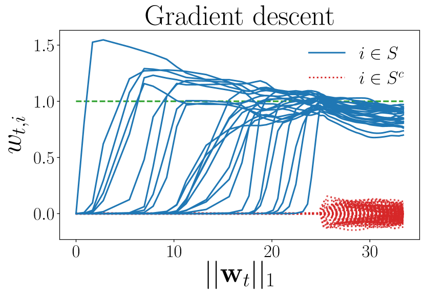
The algorithm that we propose is based on gradient descent applied to the unregularized, underdetermined objective function $\|\mathbf{X}\mathbf{w}-\mathbf{y}\|_{2}^{2}$ where $\mathbf{w}$ is parametrized as $\mathbf{w}=\mathbf{u}\odot\mathbf{u}-\mathbf{v}\odot\mathbf{v}$, with $\mathbf{u},\mathbf{v}\in\mathbb{R}^{d}$ and $\odot$ denotes the coordinate-wise multiplication operator for vectors. This parametrization yields a non-convex problem in $\mathbf{u}$ and $\mathbf{v}$. We treat this optimization problem as a proxy to design a sequence of statistical estimators that correspond to the iterates of gradient descent applied to solve the sparse regression problem, and hence are cheap to compute iteratively. The matrix formulation of the same type of parametrization that we adopt has been recently considered in the setting of low-rank matrix recovery where it leads to exact recovery via implicit regularization in the noiseless setting under the RIP [25, 30]. In our case, this choice of parametrization yields an iterative algorithm that performs multiplicative updates on the coordinates of $\mathbf{u}$ and $\mathbf{v}$, in contrast to the additive updates obtained when gradient descent is run directly on the parameter $\mathbf{w}$, as in proximal methods. This feature allows us to reduce the convergence analysis to one-dimensional iterates and to differentiate the convergence on the support set $S=\{i\in\{1,\ldots,d\}:w^{\star}_{i}\neq 0\}$ from the convergence on its complement $S^{c}=\{1,\ldots,d\}\setminus S$.

We consider gradient descent initialized with $\mathbf{u}_{0}=\mathbf{v}_{0}=\alpha\mathbf{1}$, where $\mathbf{1}$ is the all-one vector. We show that with a sufficiently small initialization size $\alpha>0$ and early stopping, our method achieves exact reconstruction with precision controlled by $\alpha$ in the noiseless setting, and minimax-optimal rates in the noisy setting. To the best of our knowledge, our results are the first to establish non-$\ell_{2}$ implicit regularization for a gradient descent method in a general noisy setting. These results rely on a constant choice of step size $\eta$ that satisfies a bound related to the unknown parameter $w^{\star}_{\max}=\|\mathbf{w}^{\star}\|_{\infty}$. We show how this choice of $\eta$ can be derived from the data itself, i.e. only based on known quantities. If the noise vector $\mathbf{\xi}$ is made up of i.i.d. sub-Gaussian components with variance proxy $\sigma^{2}$, this choice of $\eta$ yields $O((w^{\star}_{\max}\sqrt{n})/(\sigma\sqrt{\log d})\log\alpha^{-1})$ iteration complexity to achieve minimax rates. In order to achieve computational optimality, we design a preconditioned version of gradient descent (on the parameters $\mathbf{u}$ and $\mathbf{v}$) that uses increasing step-sizes and has running time $\widetilde{O}(nd)$. The iteration-dependent preconditioner relates to the statistical nature of the problem. It is made by a sequence of diagonal matrices that implement a coordinate-wise increasing step-size scheme that allows different coordinates to accelerate convergence by taking larger steps based on refined estimates of the corresponding coordinates of $\mathbf{w^{\star}}$. This algorithm yields $O(\log((w^{\star}_{\max}\sqrt{n})/(\sigma\sqrt{\log d}))\log\alpha^{-1})$ iteration complexity to achieve minimax rates in the noisy setting. Since each iteration costs $O(nd)$, the total computation complexity is, up to poly-logarithmic factors, the same as simply storing/reading the data. This algorithm is minimax-optimal and, up to logarithmic factors, computationally optimal. In contrast, we are not aware of any work on implicit $\ell_{2}$ regularization that exploits an increasing step sizes scheme in order to attain computational optimality.

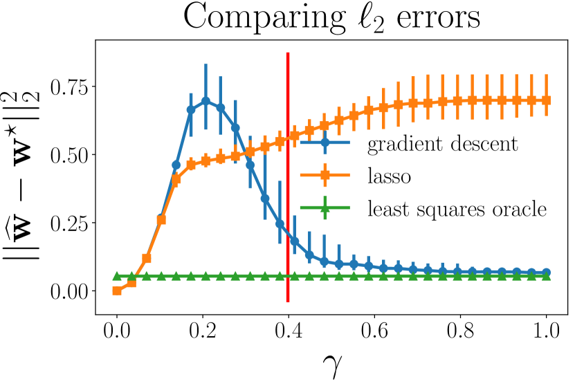
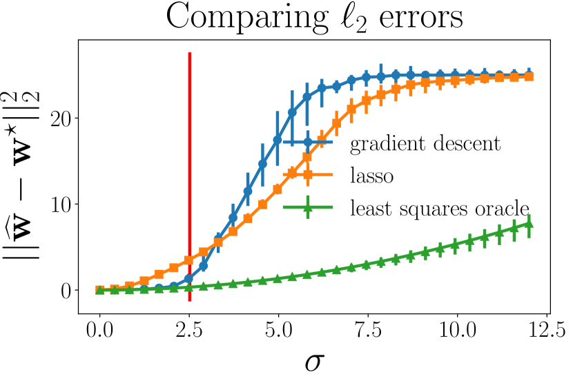
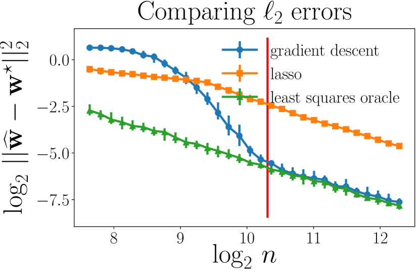
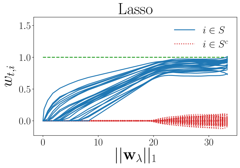
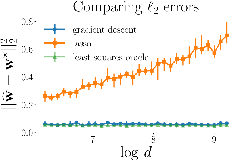
To support our theoretical results we present a simulation study of our methods and comparisons with the lasso estimator and with the gold standard oracle least squares estimator, which performs least squares regression on $S$ assuming oracle knowledge of it. We show that the number of iterations $t$ in our method plays a role similar to the lasso regularization parameter $\lambda$. Despite both algorithms being minimax-optimal with the right choice of $t$ and $\lambda$ respectively, the gradient descent optimization path—which is cheaper to compute as each iteration of gradient descent yields a new model—exhibits qualitative and quantitative differences from the lasso regularization path—which is more expensive to compute as each model requires solving a new lasso optimization program. In particular, the simulations emphasize how the multiplicative updates allow gradient descent to fit one coordinate of $\mathbf{w}^{\star}$ at a time, as opposed to the lasso estimator that tends to fit all coordinates at once. Beyond minimax results, we prove that our methods adapt to instance difficulty: for “easy” problems where the signal is greater than the noise, i.e. $w^{\star}_{\min}\gtrsim\lVert\mathbf{X}^{\mathsf{T}}\mathbf{\xi}\rVert_{\infty}/n$ with $w^{\star}_{\min}=\min_{i\in S}\left\lvert w^{\star}_{i}\right\rvert$, our estimators achieve the statistical rate $k\sigma^{2}\log(k)/n$, which does not depend on $d$. The experiments confirm this behavior and further attest that our estimators undergo a phase transition that is not observed for the lasso. Going from hard instances to easy ones, the learning capacity of implicitly-regularized gradient descent exhibits a qualitative transition and eventually matches the performance of oracle least squares.

1.2 Related Work

Sparse Recovery.

The statistical properties of explicit $\ell_{1}$ penalization techniques are well studied [48, 13, 9, 31, 33]. Minimax rates for regression under sparsity constraints are derived in [37]. Computing the whole lasso regularization path can be done via the lars algorithm [18]. Another widely used approach is the glmnet which uses cyclic coordinate-descent with warm starts to compute regularization paths for generalized linear models with convex penalties on a pre-specified grid of regularization parameters [22]. [4] reviews various optimization techniques used in solving empirical risk minimization problems with sparsity inducing penalties. Using recent advances in mixed integer optimization, [8] shows that the best subset selection problem can be tackled for problems of moderate size. For such problem sizes, comparisons between the lasso and best subset selection problem ($\ell_{0}$ regularization) were recently made, suggesting that the best subset selection performs better in high signal-to-noise ratio regimes whereas the lasso performs better when the signal-to-noise ratio is low [29]. In this sense, our empirical study in Section 5 suggests that implicitly-regularized gradient descent is more similar to $\ell_{0}$ regularization than $\ell_{1}$ regularization. Several other techniques related to $\ell_{1}$ regularization and extensions to the lasso exist. We refer the interested reader to the books [11, 47].

Implicit Regularization/Bias.

Connections between $\ell_{2}$ regularization and gradient descent optimization paths have been known for a long time and are well studied [12, 20, 52, 7, 38, 51, 34, 44, 3]. In contrast, the literature on implicit regularization inducing sparsity is scarce. Coordinate-descent optimization paths have been shown to be related to $\ell_{1}$ regularization paths in some regimes [21, 18, 40, 54]. Understanding such connections can potentially allow transferring the now well-understood theory developed for penalized forms of regularization to early-stopping-based regularization which can result in lower computational complexity. Recently, [53] have shown that neural networks generalize well even without explicit regularization despite the capacity to fit unstructured noise. This suggests that some implicit regularization effect is limiting the capacity of the obtained models along the optimization path and thus explaining generalization on structured data. Understanding such effects has recently drawn a lot of attention in the machine learning community. In particular, it is now well understood that the optimization algorithm itself can be biased towards a particular set of solutions for underdetermined problems with many global minima where, in contrast to the work cited above, the bias of optimization algorithm is investigated at or near convergence, usually in a noiseless setting [43, 27, 26, 25, 30]. We compare our assumptions with the ones made in [30] in Appendix G.

Remark 1 (Concurrent Work).

After completing this work we became aware of independent concurrent work [56] which considers Hadamard product reparametrization $\mathbf{w}_{t}=\mathbf{u}_{t}\odot\mathbf{v}_{t}$ in order to implicitly induce sparsity for linear regression under the RIP assumption. Our work is significantly different in many aspects discussed in Appendix H. In particular, we obtain computational optimality and can properly handle the general noisy setting.

2 Model and Algorithms

We consider the model defined in the introduction. We denote vectors with boldface letters and real numbers with normal font; thus, $\mathbf{w}$ denotes a vector and $w_{i}$ denotes the $i^{\mathit{th}}$ coordinate of $\mathbf{w}$. For any index set $A$ we let $\mathbf{1}_{A}$ denote a vector that has a $1$ entry in all coordinates $i\in A$ and a $0$ entry elsewhere. We denote coordinate-wise inequalities by $\preccurlyeq$. With a slight abuse of notation we write $\mathbf{w}^{2}$ to mean the vector obtained by squaring each component of $\mathbf{w}$. Finally, we denote inequalities up to multiplicative absolute constants, meaning that they do not depend on any parameters of the problem, by $\lesssim$. A table of notation can be found in Appendix I.

We now define the restricted isometry property which is the key assumption in our main theorems.

Definition 1 (Restricted Isometry Property (RIP)).

A $n\times d$ matrix $\mathbf{X}/\sqrt{n}$ satisfies the ($\delta,k$)-(RIP) if for any $k$-sparse vector $\mathbf{w}\in\mathbb{R}^{d}$ we have $(1-\delta)\left\lVert\mathbf{w}\right\rVert_{2}^{2}\leq\left\lVert\mathbf{X}\mathbf{w}/\sqrt{n}\right\rVert_{2}^{2}\leq(1+\delta)\left\lVert\mathbf{w}\right\rVert_{2}^{2}.$

The RIP assumption was introduced in [14] and is standard in the compressed sensing literature. It requires that all $n\times k$ sub-matrices of $\mathbf{X}/\sqrt{n}$ are approximately orthonormal where $\delta$ controls extent to which this approximation holds. Checking if a given matrix satisfies the RIP is NP-hard [5]. In compressed sensing applications the matrix $\mathbf{X}/\sqrt{n}$ corresponds to how we measure signals and it can be chosen by the designer of a sparse-measurement device. Random matrices are known to satisfy the RIP with high probability, with $\delta$ decreasing to $0$ as $n$ increases for a fixed $k$ [6].

We consider the following problem setting. Let $\mathbf{u},\mathbf{v}\in\mathbb{R}^{d}$ and define the mean squared loss as

$$\mathcal{L}(\mathbf{u},\mathbf{v})=\frac{1}{n}\left\lVert\mathbf{X}\left(\mathbf{u}\odot\mathbf{u}-\mathbf{v}\odot\mathbf{v}\right)-\mathbf{y}\right\rVert^{2}_{2}.$$

Letting $\mathbf{w}=\mathbf{u}\odot\mathbf{u}-\mathbf{v}\odot\mathbf{v}$ and performing gradient descent updates on $\mathbf{w}$, we recover the original parametrization of mean squared error loss which does not implicitly induce sparsity. Instead, we perform gradient descent updates on $(\mathbf{u},\mathbf{v})$ treating it as a vector in $\mathbb{R}^{2d}$ and we show that the corresponding optimization path contains sparse solutions.

Let $\eta>0$ be the learning rate, $(\mathbf{m}_{t})_{t\geq 0}$ be a sequence of vectors in $\mathbb{R}^{d}$ and $\operatorname{diag}(\mathbf{m}_{t})$ be a $d\times d$ diagonal matrix with $\mathbf{m}_{t}$ on its diagonal. We consider the following general form of gradient descent:

$$(\mathbf{u}_{t+1},\mathbf{v}_{t+1})=(\mathbf{u}_{t},\mathbf{v}_{t})-\eta\operatorname{diag}(\mathbf{m}_{t},\mathbf{m}_{t})\frac{\partial\mathcal{L}(\mathbf{u}_{t},\mathbf{v}_{t})}{\partial(\mathbf{u}_{t},\mathbf{v}_{t})}.$$ (1)

We analyze two different choices of sequences $(\mathbf{m}_{t})_{t\geq 0}$ yielding two separate algorithms.

Algorithm 1.

Let $\alpha,\eta>0$ be two given parameters. Let $\mathbf{u}_{0}=\mathbf{v}_{0}=\alpha$ and for all $t\geq 0$ we let $\mathbf{m}_{t}=\mathbf{1}$. Perform the updates given in (1).

Algorithm 2.

Let $\alpha$, $\tau\in\mathbb{N}$ and $w^{\star}_{\max}\leq\hat{z}\leq 2w^{\star}_{\max}$ be three given parameters. Set $\eta=\frac{1}{20\hat{z}}$ and $\mathbf{u}_{0}=\mathbf{v}_{0}=\alpha$. Perform the updates in (1) with $\mathbf{m}_{0}=\mathbf{1}$ and $\mathbf{m}_{t}$ adaptively defined as follows:

1. Set $\mathbf{m}_{t}=\mathbf{m}_{t-1}$.

2. If $t=m\tau\left\lceil\log\alpha^{-1}\right\rceil$ for some natural number $m\geq 2$ then let $m_{t,j}=2m_{t-1,j}$ for all $j$ such that $u_{t,j}^{2}\vee v_{t,j}^{2}\leq 2^{-m-1}\hat{z}$.

Algorithm 1 corresponds to gradient descent with a constant step size, whereas Algorithm 2 doubles the step-sizes for small enough coordinates after every $\tau\left\lceil\log\alpha^{-1}\right\rceil$ iterations.

Before stating the main results we define some key quantities. First, our results are sensitive to the condition number $\kappa=\kappa(\mathbf{w}^{\star})=w^{\star}_{\max}/w^{\star}_{\min}$ of the true parameter vector $\mathbf{w}^{\star}$. Since we are not able to recover coordinates below the maximum noise term $\lVert\mathbf{X}^{\mathsf{T}}\mathbf{\xi}\rVert_{\infty}/n$, for a desired precision $\varepsilon$ we can treat all coordinates of $\mathbf{w}^{\star}$ below $\varepsilon\vee(\lVert\mathbf{X}^{\mathsf{T}}\mathbf{\xi}\rVert_{\infty}/n)$ as $0$. This motivates the following definition of an effective condition number for given $\mathbf{w}^{\star},\mathbf{X},\xi$ and $\varepsilon$:

$$\kappa^{\text{eff}}=\kappa^{\text{eff}}(\mathbf{w}^{\star},\mathbf{X},\xi,\varepsilon)=w^{\star}_{\max}/(w^{\star}_{\min}\vee\varepsilon\vee(\lVert\mathbf{X}^{\mathsf{T}}\mathbf{\xi}\rVert_{\infty}/n)).$$

We remark that $\kappa^{\text{eff}}(\mathbf{w}^{\star},\mathbf{X},\xi,\varepsilon)\leq\kappa(\mathbf{w}^{\star})$. Second, we need to put restrictions on the RIP constant $\delta$ and initialization size $\alpha$. These restrictions are given by the following:

$$\delta(k,\mathbf{w}^{\star},\mathbf{X},\xi,\varepsilon)=1/(\sqrt{k}(1\vee\log\kappa^{\text{eff}}(\mathbf{w}^{\star}))),\quad\alpha(\mathbf{w}^{\star},\varepsilon,d)\coloneqq\frac{\varepsilon^{2}\wedge\varepsilon\wedge 1}{(2d+1)^{2}\vee(w^{\star}_{\max})^{2}}\wedge\frac{\sqrt{w^{\star}_{\min}}}{2}.$$

3 Main Results

The following result is the backbone of our contributions. It establishes rates for Algorithm 1 in the $\ell_{\infty}$ norm as opposed to the typical rates for the lasso that are often only derived for the $\ell_{2}$ norm.

Theorem 1.

Fix any $\varepsilon>0$. Suppose that $\mathbf{X}/\sqrt{n}$ satisfies the $(k+1,\delta)$-RIP with $\delta\lesssim\delta\left(k,\mathbf{w}^{\star},\mathbf{X},\xi,\varepsilon\right)$ and let the initialization $\alpha$ satisfy $\alpha\leq\alpha(\mathbf{w}^{\star},\varepsilon,d)$. Then, Algorithm 1 with $\eta\leq 1/(20w^{\star}_{\max})$ and $t=O((\kappa^{\text{eff}}(\mathbf{w}^{\star}))/(\eta w^{\star}_{\max})\log\alpha^{-1})$ iterations satisfies

$$\left\lvert w_{t,i}-w^{\star}_{i}\right\rvert \lesssim\begin{cases}\left\lVert\frac{1}{n}\mathbf{X}^{\mathsf{T}}\mathbf{\xi}\right\rVert_{\infty}\vee\varepsilon&\text{if }i\in S\text{ and }w^{\star}_{\min}\lesssim\left\lVert\frac{1}{n}\mathbf{X}^{\mathsf{T}}\mathbf{\xi}\right\rVert_{\infty}\vee\varepsilon,\\ \left\lvert\frac{1}{n}\left(\mathbf{X}^{\mathsf{T}}\mathbf{\xi}\right)_{i}\right\rvert\vee\delta\sqrt{k}\left\lVert\frac{1}{n}\mathbf{X}^{\mathsf{T}}\mathbf{\xi}\odot\mathbf{1}_{S}\right\rVert_{\infty}\vee\varepsilon&\text{if }i\in S\text{ and }w^{\star}_{\min}\gtrsim\left\lVert\frac{1}{n}\mathbf{X}^{\mathsf{T}}\mathbf{\xi}\right\rVert_{\infty}\vee\varepsilon,\\ \sqrt{\alpha}&\text{if }i\notin S.\end{cases}$$

This result shows how the parameters $\alpha,\eta$ and $t$ affect the learning performance of gradient descent. The size of $\alpha$ controls the size of the coordinates outside the true support $S$ at the stopping time. We discuss the role and also the necessity of small initialization size to achieve the desired statistical performance in Section 5. A different role is played by the step size $\eta$ whose size affects the optimal stopping time $t$. In particular, $(\eta t)/\log\alpha^{-1}$ can be seen as a regularization parameter closely related to $\lambda^{-1}$ for the lasso. To see this, suppose that the noise $\xi$ is $\sigma^{2}$-sub-Gaussian with independent components. Then with high probability $\lVert\mathbf{X}^{\mathsf{T}}\mathbf{\xi}\rVert_{\infty}/n\lesssim(\sigma\sqrt{\log d})/\sqrt{n})$. In such a setting an optimal choice of $\lambda$ for the lasso is $\Theta((\sigma\sqrt{\log d})/\sqrt{n})$. On the other hand, letting $t^{\star}$ be the optimal stopping time given in Theorem 1, we have $(\eta t^{\star})/\log\alpha^{-1}=O(1/w^{\star}_{\min}(\mathbf{X},\xi,\varepsilon))=O(\sqrt{n}/(\sigma\sqrt{\log d}))$.

The condition $\eta\leq 1/(20w^{\star}_{\max})$ is also necessary up to constant factors in order to prevent explosion. If we can set $1/w^{\star}_{\max}\lesssim\eta\leq 1/(20w^{\star}_{\max})$ then the iteration complexity of Theorem 1 reduces to $O(\kappa^{\text{eff}}(\mathbf{w}^{\star})\log\alpha^{-1})$. The magnitude of $w^{\star}_{\max}$ is, however, an unknown quantity. Similarly, setting the proper initialization size $\alpha$ depends on $w^{\star}_{\max}$, $w^{\star}_{\min}$, $d$ and the desired precision $\varepsilon$. The requirement that $\alpha\leq\sqrt{w^{\star}_{\min}}/2$ is an artifact of our proof technique and tighter analysis could replace this condition by simply $\alpha\leq\varepsilon$. Hence the only unknown quantity for selecting a proper initialization size is $w^{\star}_{\max}$.

The next theorem shows how $w^{\star}_{\max}$ can be estimated from the data up to a multiplicative factor $2$ at the cost of one gradient descent iteration. Once this estimate is computed, we can properly set the initialization size and the learning rate $\eta\asymp\frac{1}{w^{\star}_{\max}}$ which satisfies our theory and is tight up to constant multiplicative factors. We remark that $\tilde{\eta}$ used in Theorem 2 can be set arbitrarily small (e.g., set $\tilde{\eta}=10^{-10}$) and is only used for one gradient descent step in order to estimate $w^{\star}_{\max}$.

Theorem 2 (Estimating $w^{\star}_{\max}$).

Set $\alpha=1$ and suppose that $\mathbf{X}/\sqrt{n}$ satisfies the $(k+1,\delta)$-RIP with $\delta\leq 1/(20\sqrt{k}).$ Let the step size $\tilde{\eta}$ be any number satisfying $0<\tilde{\eta}\leq 1/(5w^{\star}_{\max})$ and suppose that $w^{\star}_{\max}\geq 5\lVert\mathbf{X}^{\mathsf{T}}\mathbf{\xi}\rVert_{\infty}/n$. Perform one step of gradient descent and for each $i\in\{1,\dots,d\}$ compute the update factors defined as $f^{+}_{i}=(u_{1})_{i}$ and $f^{-}_{i}=(v_{1})_{i}$. Let $f_{\max}=\left\lVert\mathbf{f}^{+}\right\rVert_{\infty}\vee\left\lVert\mathbf{f}^{-}\right\rVert_{\infty}$. Then $w^{\star}_{\max}\leq(f_{\max}-1)/(3\tilde{\eta})<2w^{\star}_{\max}.$

We present three main corollaries of Theorem 1. The first one shows that in the noiseless setting exact recovery is possible and is controlled by the desired precision $\varepsilon$ and hence by the initialization size $\alpha$.

Corollary 1 (Noiseless Recovery).

Let $\xi=0$. Under the assumptions of Theorem 1, the choice of $\eta$ given by Theorem 2 and $t=O(\kappa^{\text{eff}}(\mathbf{w}^{\star})\log\alpha^{-1})$, Algorithm 1 yields $\left\lVert\mathbf{w}_{t}-\mathbf{w}^{\star}\right\rVert_{2}^{2}\lesssim k\varepsilon^{2}$.

In the general noisy setting exact reconstruction of $\mathbf{w}^{\star}$ is not possible. In fact, the bounds in Theorem 1 do not improve with $\varepsilon$ chosen below the maximum noise term $\lVert\mathbf{X}^{\mathsf{T}}\mathbf{\xi}\rVert_{\infty}/n$. In the following corollary we show that with a small enough $\varepsilon$ if the design matrix $\mathbf{X}$ is fixed and the noise vector $\xi$ is sub-Gaussian, we recover minimax-optimal rates for $\ell_{2}$ error. Our error bound is minimax-optimal in the setting of sub-linear sparsity, meaning that there exists a constant $\gamma>1$ such that $k^{\gamma}\leq d$.

Corollary 2 (Minimax Rates in the Noisy Setting).

Let the noise vector $\xi$ be made of independent $\sigma^{2}$-sub-Gaussian entries. Let $\varepsilon=4\sqrt{\sigma^{2}\log(2d)}/\sqrt{n}$. Under the assumptions of Theorem 1, the choice of $\eta$ given by Theorem 2 and $t=O(\kappa^{\text{eff}}(\mathbf{w}^{\star})\log\alpha^{-1})=O((w^{\star}_{\max}\sqrt{n})/(\sigma\sqrt{\log d})\log\alpha^{-1})$, Algorithm 1 yields $\left\lVert\mathbf{w}_{t}-\mathbf{w}^{\star}\right\rVert_{2}^{2}\lesssim(k\sigma^{2}\log d)/n$ with probability at least $1-1/(8d^{3})$.

The next corollary states that gradient descent automatically adapts to the difficulty of the problem. The statement of Theorem 1 suggests that our bounds undergo a phase-transition when $w^{\star}_{\min}\gtrsim\lVert\mathbf{X}^{\mathsf{T}}\mathbf{\xi}\rVert_{\infty}/n$ which is also supported by our empirical findings in Section 5. In the $\sigma^{2}$-sub-Gaussian noise setting the transition occurs as soon as $n\gtrsim(\sigma^{2}\log d)/(w^{\star}_{\min})^{2}$. As a result, the statistical bounds achieved by our algorithm are independent of $d$ in such a setting. To see that, note that while the term $\lVert\mathbf{X}^{\mathsf{T}}\mathbf{\xi}\rVert_{\infty}/n$ grows as $O(\log d)$, the term $\lVert\mathbf{X}^{\mathsf{T}}\mathbf{\xi}\odot\mathbf{1}_{S}\rVert_{\infty}/n$ grows only as $O(\log k)$. In contrast, performance of the lasso deteriorates with $d$ regardless of the difficulty of the problem. We illustrate this graphically and give a theoretical explanation in Section 5. We remark that the following result does not contradict minimax optimality because we now treat the true parameter $\mathbf{w}^{\star}$ as fixed.

Corollary 3 (Instance Adaptivity).

Let the noise vector $\xi$ be made of independent $\sigma^{2}$-sub-Gaussian entries. Let $\varepsilon=4\sqrt{\sigma^{2}\log(2k)}/\sqrt{n}$. Under the assumptions of Theorem 1, the choice of $\eta$ given by Theorem 2 and $t=O(\kappa^{\text{eff}}(\mathbf{w}^{\star})\log\alpha^{-1})=O((w^{\star}_{\max}\sqrt{n})/(\sigma\sqrt{\log k})\log\alpha^{-1})$, Algorithm 1 yields $\left\lVert\mathbf{w}_{t}-\mathbf{w}^{\star}\right\rVert_{2}^{2}\lesssim(k\sigma^{2}\log k)/n$. with probability at least $1-1/(8k^{3})$.

The final theorem we present shows that the same statistical bounds achieved by Algorithm 1 are also attained by Algorithm 2. This algorithm is not only optimal in a statistical sense, but it is also optimal computationally up to poly-logarithmic factors.

Theorem 3.

Compute $\hat{z}$ using Theorem 2. Under the setting of Theorem 1 there exists a large enough absolute constant $\tau$ so that Algorithm 2 parameterized with $\alpha,\tau$ and $\hat{z}$ satisfies the result of Theorem 1 and $t=O(\log\kappa^{\text{eff}}\log\alpha^{-1})$ iterations.

Corollaries 1, 2 and 3 also hold for Algorithm 2 with stopping time equal to $O(\log\kappa^{\text{eff}}\log\alpha^{-1})$. We emphasize that both Theorem 1 and 3 use gradient-based updates to obtain a sequence of models with optimal statistical properties instead of optimizing the objective function $\mathcal{L}$. In fact, if we let $t\to\infty$ for Algorithm 2 the iterates would explode.

4 Proof Sketch

In this section we prove a simplified version of Theorem 1 under the assumption $\mathbf{X}^{\mathsf{T}}\mathbf{X}/n=\mathbf{I}$. We further highlight the intricacies involved in the general setting and present the intuition behind the key ideas there. The gradient descent updates on $\mathbf{u}_{t}$ and $\mathbf{v}_{t}$ as given in (1) can be written as

$$\begin{split}\mathbf{u}_{t+1}=\mathbf{u}_{t}\odot\left(\mathbf{1}-(4\eta/n)\mathbf{X}^{\mathsf{T}}(\mathbf{X}\mathbf{w}_{t}-\mathbf{y})\right),&\quad\mathbf{v}_{t+1}=\mathbf{v}_{t}\odot\left(\mathbf{1}+({4\eta}/{n})\mathbf{X}^{\mathsf{T}}(\mathbf{X}\mathbf{w}_{t}-\mathbf{y})\right).\end{split}$$ (2)

The updates can be succinctly represented as $\mathbf{u}_{t+1}=\mathbf{u}_{t}\odot(\mathbf{1}-\mathbf{r})$ and $\mathbf{v}_{t+1}=\mathbf{v}_{t}\odot(\mathbf{1}+\mathbf{r})$, where by our choice of $\eta$, $\left\lVert\mathbf{r}\right\rVert_{\infty}\leq 1$. Thus, $(\mathbf{1}-\mathbf{r})\odot(\mathbf{1}+\mathbf{r})\preccurlyeq\mathbf{1}$ and we have $\mathbf{u}_{t}\odot\mathbf{v}_{t}\preccurlyeq\mathbf{u}_{0}\odot\mathbf{v}_{0}=\alpha^{2}\mathbf{1}$. Hence for any $i$, only one of $|u_{t,i}|$ and $|v_{t,i}|$ can be larger then the initialization size while the other is effectively equal to $0$. Intuitively, $u_{t,i}$ is used if $w^{\star}_{i}>0$, $v_{t,i}$ if $w^{\star}_{i}<0$ and hence one of these terms can be merged into an error term $b_{t,i}$ as defined below. The details appear in Appendix B.4. To avoid getting lost in cumbersome notation, in this section we will assume that $\mathbf{w}^{\star}\succcurlyeq 0$ and $\mathbf{w}=\mathbf{u}\odot\mathbf{u}$.

Theorem 4.

Assume that $\mathbf{w}^{\star}\succcurlyeq\mathbf{0}$, $\frac{1}{n}\mathbf{X}^{\mathsf{T}}\mathbf{X}=\mathbf{I}$, and that there is no noise ($\mathbf{\xi}=0$). Parameterize $\mathbf{w}=\mathbf{u}\odot\mathbf{u}$ with $\mathbf{u}_{0}=\alpha\mathbf{1}$ for some $0<\alpha<\sqrt{w^{\star}_{\min}}$. Letting $\eta\leq 1/(10w^{\star}_{\max})$ and $t=O(\log(w^{\star}_{\max}/\alpha^{2})/(\eta w^{\star}_{\min}))$, Algorithm 1 yields $\lVert\mathbf{w}_{t}-\mathbf{w}^{\star}\rVert_{\infty}\leq\alpha^{2}$.

Proof.

As $\mathbf{X}^{\mathsf{T}}\mathbf{X}/n=\mathbf{I},\mathbf{y}=\mathbf{X}\mathbf{w}^{\star}$, and $\mathbf{v}_{t}=\mathbf{0}$, the updates given in equation (2) reduce component-wise to updates on $\mathbf{w}_{t}$ given by $w_{t+1,i}=w_{t,i}\cdot(1-4\eta(w_{t,i}-w^{\star}_{i}))^{2}.$ For $i$ such that $w^{\star}_{i}=0$, $w_{t,i}$ is non-increasing and hence stays below $\alpha^{2}$. For $i$ such that $w^{\star}_{i}>\alpha^{2}$, the update rule given above ensures that as long as $w_{t,i}<w^{\star}_{i}/2$, $w_{t,i}$ increases at an exponential rate with base at least $(1+2\eta w^{\star}_{i})^{2}$. As $w_{0,i}=\alpha^{2}$, in $O(\log(w^{\star}_{i}/\alpha^{2})/(\eta w^{\star}_{i}))$ steps, it holds that $w_{t,i}\geq w^{\star}_{i}/2$. Subsequently, the gap $(w^{\star}_{i}-w_{t,i})$ halves every $O(1/\eta w^{\star}_{i})$ steps; thus, in $O(\log(w^{\star}_{\max}/\alpha^{2})/(\eta w^{\star}_{\min}))$ steps we have $\lVert\mathbf{w}_{t}-\mathbf{w}^{\star}\rVert_{\infty}\leq\alpha^{2}$. The exact details are an exercise in calculus, albeit a rather tedious one, and appear in Appendix B.1. ∎

The proof of Theorem 4 contains the key ideas of the proof of Theorem 1. However, the presence of noise ($\mathbf{\xi}\neq 0$) and only having restricted isometry of $\mathbf{X}^{\mathsf{T}}\mathbf{X}$ rather than isometry requires a subtle and involved analysis. We remark that we can prove tighter bounds in Theorem 4 than the ones in Theorem 1 because we are working in a simplified setting.

Error Decompositions.

We decompose $\mathbf{w}_{t}$ into $\mathbf{s}_{t}\coloneqq\mathbf{w}_{t}\odot\mathbf{1}_{S}$ and $\mathbf{e}_{t}\coloneqq\mathbf{w}_{t}\odot\mathbf{1}_{S^{c}}$ so that $\mathbf{w}_{t}=\mathbf{s}_{t}+\mathbf{e}_{t}$. We define the following error sequences:

$$\mathbf{b}_{t}={\mathbf{X}^{\mathsf{T}}\mathbf{X}}\mathbf{e}_{t}/n+{\mathbf{X}^{\mathsf{T}}\mathbf{\xi}}/{n}, \qquad\mathbf{p}_{t}=\left({\mathbf{X}^{\mathsf{T}}\mathbf{X}}/{n}-\mathbf{I}\right)(\mathbf{s}_{t}-\mathbf{w}^{\star}),$$

which allows us to write updates on $\mathbf{s}_{t}$ and $\mathbf{e}_{t}$ as

$$\mathbf{s}_{t+1}=\mathbf{s}_{t}\odot(1-4\eta(\mathbf{s}_{t}-\mathbf{w}^{*}+\mathbf{p}_{t}+\mathbf{b}_{t}))^{2},\qquad\mathbf{e}_{t+1}=\mathbf{e}_{t}\odot(1-4\eta(\mathbf{p}_{t}+\mathbf{b}_{t}))^{2}.$$

Error Sequence $\mathbf{b}_{t}$.

Since our theorems require stopping before $\left\lVert\mathbf{e}_{t}\right\rVert_{\infty}$ exceeds $\sqrt{\alpha}$, the term $\mathbf{X}^{\mathsf{T}}\mathbf{X}\mathbf{e}_{t}/n$ can be controlled entirely by the initialization size. Hence $\mathbf{b}_{t}\approx\mathbf{X}^{\mathsf{T}}\mathbf{\xi}/n$ and it represents an irreducible error arising due to the noise on the labels. For any $i\in S$ at stopping time $t$ we cannot expect the error on the $i^{\mathit{th}}$ coordinate $\lvert w_{t,i}-w^{\star}_{i}\rvert$ to be smaller than $\lvert(\mathbf{X}^{\mathsf{T}}\mathbf{\xi})/n)_{i}\rvert$. If we assume $\mathbf{p}_{t}=0$ and $\xi\neq 0$ then in light of our simplified Theorem 4 we see that the terms in $\mathbf{e}_{t}$ grow exponentially with base at most $(1+4\eta\lVert\mathbf{X}^{\mathsf{T}}\mathbf{\xi}\rVert_{\infty}/n)$. We can fit all the terms in $\mathbf{s}_{t}$ such that $\lvert w^{\star}_{i}\rvert\gtrsim\lVert\mathbf{X}^{\mathsf{T}}\mathbf{\xi}\rVert_{\infty}/n$ which leads to minimax-optimal rates. Moreover, if $w^{\star}_{\min}\gtrsim\lVert\mathbf{X}^{\mathsf{T}}\mathbf{\xi}\rVert_{\infty}/n$ then all the elements in $\mathbf{s}_{t}$ grow exponentially at a faster rate than all of the error terms. This corresponds to the easy setting where the resulting error depends only on $\lVert\mathbf{X}^{\mathsf{T}}\mathbf{\xi}/n\odot\mathbf{1}_{S}\rVert_{\infty}$ yielding dimension-independent error bounds. For more details see Appendix B.2.

Error Sequence $\mathbf{p}_{t}$.

Since $\mathbf{s}_{t}-\mathbf{w}^{\star}$ is a $k$-sparse vector using the RIP we can upper-bound $\left\lVert\mathbf{p}_{t}\right\rVert_{\infty}\leq\sqrt{k}\delta\left\lVert\mathbf{s}_{t}-\mathbf{w}^{\star}\right\rVert_{\infty}$. Note that for small $t$ we have $\left\lVert\mathbf{s}_{0}\right\rVert_{\infty}\approx\alpha^{2}\approx 0$ and hence, ignoring the logarithmic factor in the definition of $\delta$ in the worst case we have $Cw^{\star}_{\max}\leq\left\lVert\mathbf{p}_{t}\right\rVert_{\infty}<w^{\star}_{\max}$ for some absolute constant $0<C<1$. If $w^{\star}_{\max}\gg\lVert\mathbf{X}^{\mathsf{T}}\mathbf{\xi}\rVert_{\infty}/n$ then the error terms can grow exponentially with base $(1+4\eta\cdot Cw^{\star}_{\max})$ whereas the signal terms such that $\lvert w^{\star}_{i}\rvert\ll w^{\star}_{\max}$ can shrink exponentially at rate $(1-4\eta\cdot Cw^{\star}_{\max})$. On the other hand, in the light of Theorem 4 the signal elements converge exponentially fast to the true parameters $w^{\star}_{\max}$ and hence the error sequence $\mathbf{p}_{t}$ should be exponentially decreasing. For small enough $C$ and a careful choice of initialization size $\alpha$ we can ensure that elements of $\mathbf{p}_{t}$ decrease before the error components in $\mathbf{e}_{t}$ get too large or the signal components in $\mathbf{s}_{t}$ get too small. For more details see Appendix A.2 and B.3.

Tuning Learning Rates.

The proof of Theorem 2 is given in Appendix D. If we choose $1/w^{\star}_{\max}\lesssim\eta\leq 1/(10w^{\star}_{\max})$ in Theorem 4 then all coordinates converge in $O(\kappa\log(w^{\star}_{\max}/\alpha^{2}))$ iterations. The reason the factor $\kappa$ appears is the need to ensure that the convergence of the component $w^{\star}_{i}=w^{\star}_{\max}$ is stable. However, this conservative setting of the learning rate unnecessarily slows down the convergence for components with $w^{\star}_{i}\ll w^{\star}_{\max}$. In Theorem 4, oracle knowledge of $\mathbf{w}^{\star}$ would allow to set an individual step size for each coordinate $i\in S$ equal to $\eta_{i}=1/(10w^{\star}_{i})$ yielding the total number of iterations equal to $O(\log(w^{\star}_{\max}/\alpha^{2}))$. In the setting where $\mathbf{X}^{\mathsf{T}}\mathbf{X}/n\neq\mathbf{I}$ this would not be possible even with the knowledge of $\mathbf{w}^{\star}$, since the error sequence $\mathbf{p}_{t}$ can be initially too large which would result in explosion of the coordinates $i$ with $\lvert w^{\star}_{i}\rvert\ll w^{\star}_{\max}$. Instead, we need to wait for $\mathbf{p}_{t}$ to get small enough before we increase the step size for some of the coordinates as described in Algorithm 2. The analysis is considerably involved and the full proof can be found in Appendix E. We illustrate effects of increasing step sizes in Section 5.

5 Simulations

Unless otherwise specified, the default simulation set up is as follows. We let $\mathbf{w}^{\star}=\gamma\mathbf{1}_{S}$ for some constant $\gamma$. For each run the entries of $\mathbf{X}$ are sampled as i.i.d. Rademacher random variables and the noise vector $\mathbf{\xi}$ follows i.i.d. $N(0,\sigma^{2})$ distribution. For $\ell_{2}$ plots each simulation is repeated a total of $30$ times and the median $\ell_{2}$ error is depicted. The error bars in all the plots denote the $25^{\mathit{th}}$ and $75^{\mathit{th}}$ percentiles. Unless otherwise specified, the default values for simulation parameters are $n=500,d=10^{4},k=25,\alpha=10^{-12},\gamma=1,\sigma=1$ and for Algorithm 2 we set $\tau=10$.

Effects of Initialization Size.

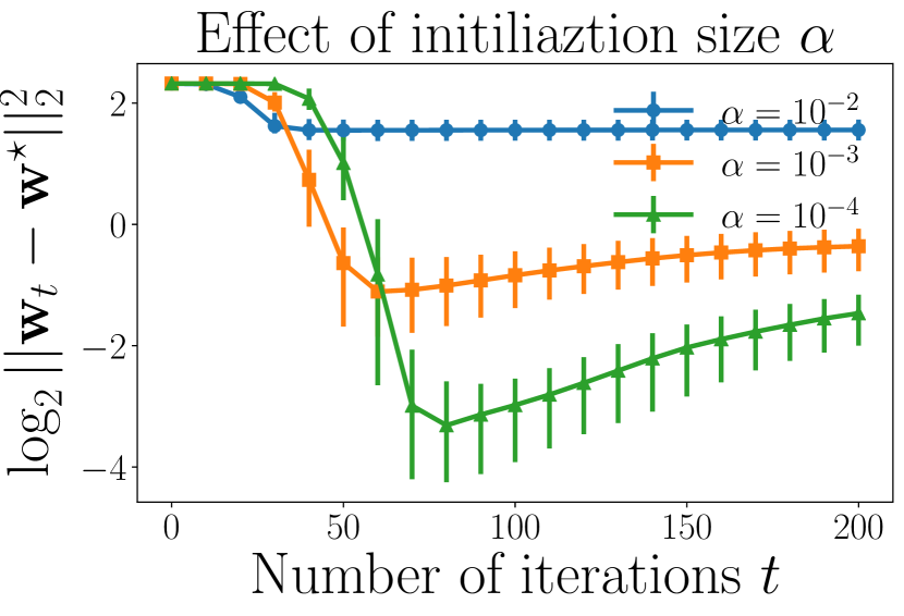
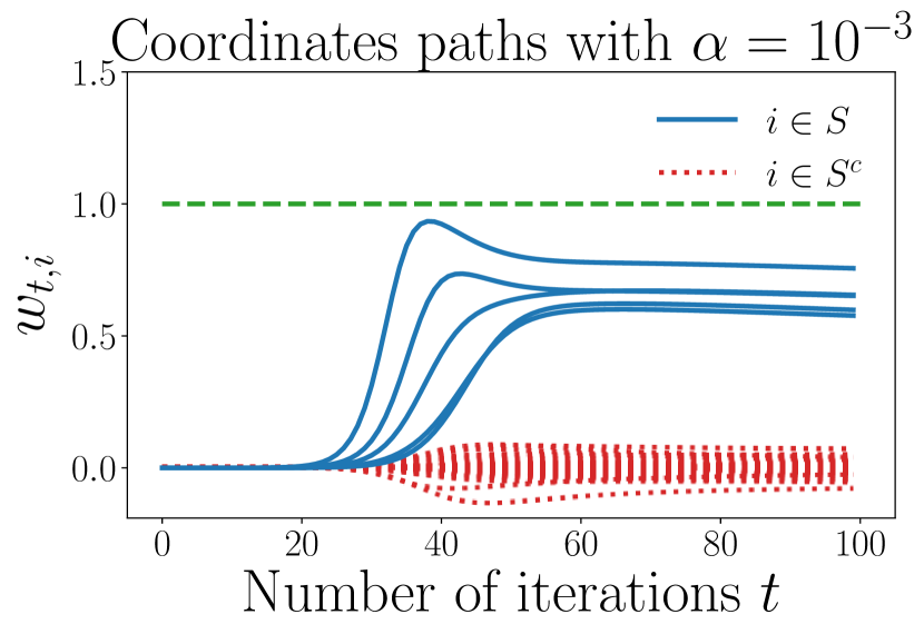
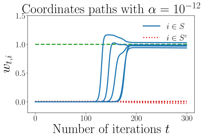
As discussed in Section 4 each coordinate grows exponentially at a different rate. In Figure 1 we illustrate the necessity of small initialization for bringing out the exponential nature of coordinate paths allowing to effectively fit them one at a time. For more intuition, suppose that coordinates outside the true support grow at most as fast as $(1+\varepsilon)^{t}$ while the coordinates on the true support grow at least as fast as $(1+2\varepsilon)^{t}$. Since exponential function is very sensitive to its base, for large enough $t$ we have $(1+\varepsilon)^{t}\ll(1+2\varepsilon)^{t}$. The role of the initialization size $\alpha$ is then finding a small enough $\alpha$ such that for large enough $t$ we have $\alpha^{2}(1+\varepsilon)^{t}\approx 0$ while $\alpha^{2}(1+2\varepsilon)^{t}$ is large enough to ensure convergence of the coordinates on the true support.

Figure 1: Effects of initialization size. We set $k=5,n=100,\eta=0.05,\sigma=0.5$ and run Algorithm 1. We remark that the $X$ axes in the two figures on the right differ due to different choices of $\alpha$.

Exponential Convergence with Increasing Step Sizes.

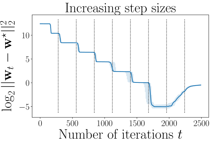
We illustrate the effects of Algorithm 2 on an ill-conditioned target with $\kappa=64$. Algorithm 1 spends approximately twice the time to fit each coordinate that the previous one, which is expected, since the coordinate sizes decrease by half. On the other hand, as soon as we increase the corresponding step size, Algorithm 2 fits each coordinate at approximately the same number of iterations, resulting in $O(\log\kappa\log\alpha^{-1})$ total iterations. Figure 2 confirms this behavior in simulations.

Figure 2: Comparison of Algorithms 1 and 2. Let $n=250,k=7$ and the non-zero coordinates of $\mathbf{w}^{\star}$ be $\{2^{i}:i=0,\dots,6\}$. For both algorithms let $\eta=1/(20\cdot 2^{6})$. The vertical lines in the figure on the right are equally spaced at $\tau\log\alpha^{-1}$ iterations. The scale of x axes differ by a factor of $16$. The shaded region corresponds to $25^{\mathit{th}}$ and $75^{\mathit{th}}$ percentiles over $30$ runs.

Phase Transitions.

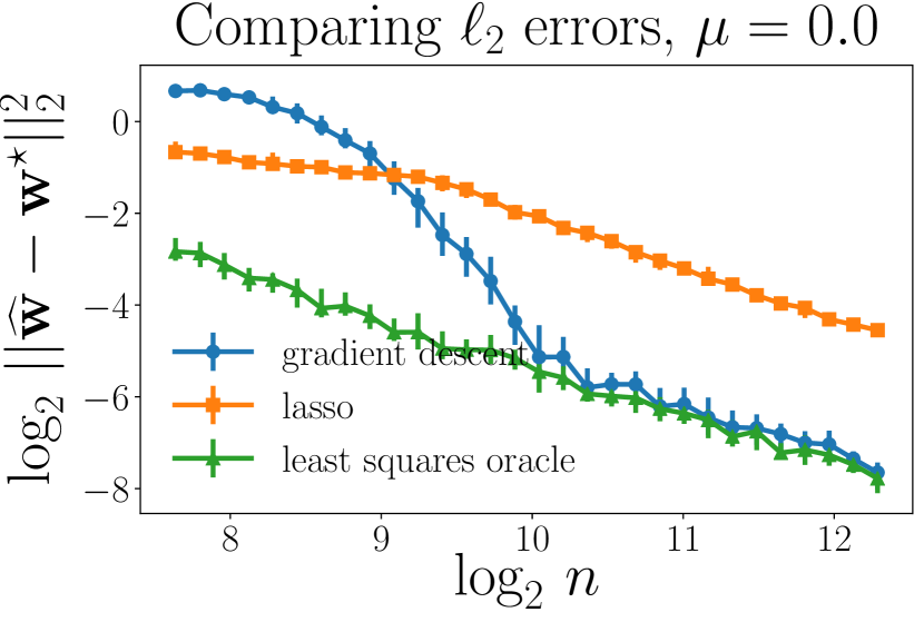
As suggested by our main results, we present empirical evidence that when $w^{\star}_{\min}\gtrsim\lVert\mathbf{X}^{\mathsf{T}}\mathbf{\xi}\rVert_{\infty}/n$ our algorithms undergo a phase transition with dimension-independent error bounds. We plot results for three different estimators. First we run Algorithm 2 for $2000$ iterations and save every $10^{\mathit{th}}$ model. Among the $200$ obtained models we choose the one with the smallest error on a validation dataset of size $n/4$. We run the lasso for $200$ choices of $\lambda$ equally spaced on a logarithmic scale and for each run we select a model with the smallest $\ell_{2}$ parameter estimation error using an oracle knowledge of $\mathbf{w}^{\star}$. Finally, we perform a least squares fit using an oracle knowledge of the true support $S$. Figure 3 illustrates, that with varying $\gamma,\sigma$ and $n$ we can satisfy the condition $w^{\star}_{\min}\gtrsim\lVert\mathbf{X}^{\mathsf{T}}\mathbf{\xi}\rVert_{\infty}/n$ at which point our method approaches an oracle-like performance. Given exponential nature of the coordinate-wise convergence, all coordinates of the true support grow at a strictly larger exponential rate than all of the coordinates on $S^{c}$ as soon as $w^{\star}_{\min}-\lVert\mathbf{X}^{\mathsf{T}}\mathbf{\xi}\rVert_{\infty}/n>\lVert\mathbf{X}^{\mathsf{T}}\mathbf{\xi}\rVert_{\infty}/n$. An approximate solution of this equation is shown in Figure 3 using vertical red lines.

Figure 3: Phase transitions. The figure on the right uses $\gamma=1/4$. The red vertical lines show solutions of the equation $w^{\star}_{\min}=\gamma=2\cdot\mathbb{E}\!\left[{\lVert\mathbf{X}^{\mathsf{T}}\mathbf{\xi}\rVert_{\infty}/n}\right]\leq 2\cdot\sigma\sqrt{2\log(2d)}/\sqrt{n}.$

Dimension Free Bounds in the Easy Setting.

Figure 4 shows that when $w^{\star}_{\min}\gtrsim\lVert\mathbf{X}^{\mathsf{T}}\mathbf{\xi}\rVert_{\infty}/n$ our algorithm matches the performance of oracle least squares which is independent of $d$. In contrast, the performance of the lasso deteriorates as $d$ increases. To see why this is the case, in the setting where $\mathbf{X}^{\mathsf{T}}\mathbf{X}/n=\mathbf{I}$, the lasso solution with parameter $\lambda$ has a closed form solution $w^{\lambda}_{i}=\mathrm{sign}(w^{\textsc{LS}}_{i})(|w^{\textsc{LS}}_{i}|-\lambda)_{+}$, where $\mathbf{w}^{\textsc{LS}}$ is the least squares solution. In the sub-Gaussian noise setting, the minimax rates are achieved by the choice $\lambda=\Theta(\sqrt{\sigma^{2}\log(d)/n})$ introducing a bias which depends on $\log d$. Such a bias is illustrated in Figure 4 and is not present at the optimal stopping time of our algorithm.

Figure 4: Dimension dependent bias for the lasso. In contrast, in a high signal-to-noise ratio setting gradient descent is able to recover coordinates on $S$ without a visible bias.

6 Further Improvements

While we show that Algorithms 1 and 2 yield optimal statistical rates and in addition Algorithm 2 is optimal in terms of computational requirements, our results can be improved in two different aspects. First, our constraints on the RIP parameter $\delta$ result in sub-optimal sample complexity. Second, the RIP condition could potentially be replaced by the restricted eigenvalue (RE) condition which allows correlated designs. We expand on both of the points below and provide empirical evidence suggesting that both inefficiencies are artifacts of our analysis and not inherent limitations of our algorithms.

Sub-Optimal Sample Complexity. Our RIP parameter $\delta$ scales as $\widetilde{O}(1/\sqrt{k})$. We remark that such scaling on $\delta$ is less restrictive than in [30, 56] (see Appendix G and H). If we consider, for example, sub-Gaussian isotropic designs, then satisfying such an assumption requires $n\gtrsim k^{2}\log(ed/k)$ samples. To see that, consider an $n\times k$ i.i.d. standard normal ensemble which we denote by $\mathbf{X}$. By standard results in random-matrix theory [50, Chapter 6], $\lVert\mathbf{X}^{\mathsf{T}}\mathbf{X}/n-\mathbf{I}\rVert\lesssim\sqrt{k/n}+k/n$ where $\left\lVert\cdot\right\rVert$ denotes the operator norm. Hence, we need $n\gtrsim k^{2}$ to satisfy $\lVert\mathbf{X}^{\mathsf{T}}\mathbf{X}/n-\mathbf{I}\rVert\lesssim 1/\sqrt{k}$.

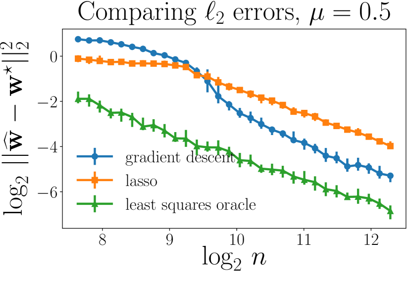
Note that Theorems 1 and 3 provide coordinate-wise bounds which is in general harder than providing $\ell_{2}$ error bounds directly. In particular, under the condition that $\delta=\widetilde{O}(1/\sqrt{k})$, our main theorems imply minimax-optimal $\ell_{2}$ bounds; this requirement on $\delta$ implies that $n$ needs to be at least quadratic in $k$. Hence we need to answer two questions. First, do we need sample complexity quadratic in $k$ to obtain minimax-rates? The left plot in Figure 5 suggests that linear sample complexity in $k$ is enough for our method to match and eventually exceed performance of the lasso in terms of $\ell_{2}$ error. Second, is it necessary to change our $\ell_{\infty}$ based analysis to an $\ell_{2}$ based analysis in order to obtain optimal sample complexity? The right plot in Figure 5 once again suggests that sample complexity linear in $k$ is enough for our main theorems to hold.

Figure 5: Sample complexity requirements. We let $d=5000,\sigma=1$ and $\mathbf{w}^{\star}_{S}=\mathbf{1}_{S}$. The plot on the left computes the $\log_{2}$ error ratio for our method (stopping time chosen by cross-validation) and the lasso ($\lambda$ chosen optimally using knowledge of $\mathbf{w}^{\star}$). The plot on the right computes $\lVert\mathbf{w}_{t}\odot\mathbf{1}_{S^{c}}\rVert_{\infty}$ for optimally chosen $t$.

Relaxation to the Restricted Eigenvalue (RE) Assumption. The RIP assumption is crucial for our analysis. However, the lasso satisfies minimax optimal rates under less restrictive assumptions, namely, the RE assumption introduced in [9]. The RE assumption with parameter $\gamma$ requires that $\lVert\mathbf{X}\mathbf{w}\rVert_{2}^{2}/n\geq\gamma\lVert\mathbf{w}\rVert_{2}^{2}$ for vectors $\mathbf{w}$ satisfying the cone condition $\lVert\mathbf{w}_{S^{c}}\rVert_{1}\leq c\lVert\mathbf{w}_{S}\rVert_{1}$ for a suitable choice of constant $c\geq 1$. In contrast to RIP, RE only imposes constraints on the lower eigenvalue of $\mathbf{X}^{\mathsf{T}}\mathbf{X}/n$ for approximately sparse vectors and can be satisfied by random correlated designs [36, 42]. The RE condition was shown to be necessary for any polynomial-time algorithm returning a sparse vector and achieving fast rates for prediction error [55].

We sample i.i.d. Gaussian ensembles with covariance matrices equal to $(1-\mu)\mathbf{I}+\mu\mathbf{1}\mathbf{1}^{\mathsf{T}}$ for $\mu=0$ and $0.5$. For $\mu=0.5$ the RIP fails but the RE property holds with high probability [50, Chapter 7]. In Figure 6 we show empirically that our method achieves the fast rates and eventually outperforms the lasso even when we violate the RIP assumption.

Figure 6: Violating the RIP assumption. We consider the same setting as in Figure 3 with rows of $\mathbf{X}$ sampled from a Gaussian distribution with covariance matrix equal to $(1-\mu)\mathbf{I}+\mu\mathbf{1}\mathbf{1}^{\mathsf{T}}$.

Appendix

The appendix is organized as follows.

In Appendix A we introduce the key ideas and intuition behind the proof of Theorem 1.

In Appendix B we go deeper into technical details and prove the main propositions used to prove Theorem 1.

In Appendix C we prove the lemmas stated in appendix A.

In Appendix D we prove Theorem 2.

In Appendix E we prove Theorem 3.

In Appendix F we derive the gradient descent updates used by our parametrization.

In Appendix G we compare our assumptions with the ones made in [30].

In Appendix H we compare our main result with a recent arXiv preprint [56], where Hadamard product reparametrization was used to induce sparsity implicitly.

In Appendix I we provide a table of notation.

Appendix A Proof of Theorem 1

This section is dedicated to providing a high level proof for Theorem 1. In Section A.1 we set up the notation and explain how we decompose our iterates into signal and error sequences. In Section A.2 we state and discuss the implications of the two key propositions allowing to prove our theorem. In Section A.3 we state some technical lemmas used in the proofs of the main theorem and its corollaries. In Section A.4 we prove Theorem 1. Finally in Section A.5 we prove the corollaries.

A.1 Set Up and Intuition

Let $\mathbf{w}_{t}\coloneqq\mathbf{w}_{t}^{+}-\mathbf{w}_{t}^{-}$ where $\mathbf{w}_{t}^{+}\coloneqq\mathbf{u}_{t}\odot\mathbf{u}_{t}$ and $\mathbf{w}_{t}^{-}\coloneqq\mathbf{v}_{t}\odot\mathbf{v}_{t}$. The gradient descent updates on $\mathbf{u}_{t}$ and $\mathbf{v}_{t}$ read as (see Appendix F for derivation)

$$\mathbf{u}_{t+1} =\mathbf{u}_{t}\odot\left(\mathbf{1}-4\eta\left(\frac{1}{n}\mathbf{X}^{\mathsf{T}}(\mathbf{X}(\mathbf{w}_{t}-\mathbf{w}^{\star})-\mathbf{\xi})\right)\right),$$

$$\mathbf{v}_{t+1} =\mathbf{v}_{t}\odot\left(\mathbf{1}+4\eta\left(\frac{1}{n}\mathbf{X}^{\mathsf{T}}(\mathbf{X}(\mathbf{w}_{t}-\mathbf{w}^{\star})-\mathbf{\xi})\right)\right).$$

Let $S^{+}$ denote the coordinates of $\mathbf{w}^{\star}$ such that $w^{\star}_{i}>0$ and let $S^{-}$ denote the coordinates of $\mathbf{w}^{\star}$ such that $w^{\star}_{i}<0$. So $S=S^{+}\cup S^{-}$ and $S^{+}\cap S^{-}=\emptyset$. Then define the following sequences

$$\begin{split}\mathbf{s}_{t}&\coloneqq\mathbf{1}_{S^{+}}\odot\mathbf{w}_{t}^{+}-\mathbf{1}_{S^{-}}\odot\mathbf{w}_{t}^{-},\\ \mathbf{e}_{t}&\coloneqq\mathbf{1}_{S^{c}}\odot\mathbf{w}_{t}+\mathbf{1}_{S^{-}}\odot\mathbf{w}_{t}^{+}-\mathbf{1}_{S^{+}}\odot\mathbf{w}_{t}^{-},\\ \mathbf{b}_{t}&\coloneqq\frac{1}{n}\mathbf{X}^{\mathsf{T}}\mathbf{X}\mathbf{e}_{t}-\frac{1}{n}\mathbf{X}^{\mathsf{T}}\mathbf{\xi},\\ \mathbf{p}_{t}&\coloneqq\left(\frac{1}{n}\mathbf{X}^{\mathsf{T}}\mathbf{X}-\mathbf{I}\right)\left(\mathbf{s}_{t}-\mathbf{w}^{\star}\right).\end{split}$$ (3)

Having defined the sequences above we can now let $\alpha^{2}$ be the initialization size and rewrite the updates on $\mathbf{w}_{t}$, $\mathbf{w}_{t}^{+}$ and $\mathbf{w}_{t}^{-}$ in a more succinct way

$$\begin{split}\mathbf{w}_{0}^{+}&=\mathbf{w}_{0}^{-}=\alpha^{2},\\ \mathbf{w}_{t}&=\mathbf{w}_{t}^{+}-\mathbf{w}_{t}^{-}\\ \mathbf{w}_{t+1}^{+}&=\mathbf{w}_{t}^{+}\odot\left(\mathbf{1}-4\eta\left(\mathbf{s}_{t}-\mathbf{w}^{\star}+\mathbf{p}_{t}+\mathbf{b}_{t}\right)\right)^{2},\\ \mathbf{w}_{t+1}^{-}&=\mathbf{w}_{t}^{-}\odot\left(\mathbf{1}+4\eta\left(\mathbf{s}_{t}-\mathbf{w}^{\star}+\mathbf{p}_{t}+\mathbf{b}_{t}\right)\right)^{2}.\end{split}$$ (4)

We will now explain the roles played by each sequence defined in equation (3).

1. The sequence $(\mathbf{s}_{t})_{t\geq 0}$ represents the signal that we have fit by iteration $t$. In the noiseless setting, $\mathbf{s}_{t}$ would converge to $\mathbf{w}^{\star}$. We remark that $\mathbf{w}_{t}^{+}$ is responsible for fitting the positive components of $\mathbf{w}^{\star}$ while $\mathbf{w}_{t}^{-}$ is responsible for fitting the negative components of $\mathbf{w}^{\star}$. If we had the knowledge of $S^{+}$ and $S^{-}$ before starting our algorithm, we would set $\mathbf{w}_{0}$ to $\mathbf{s}_{0}$.

2. The sequence $(\mathbf{e}_{t})_{t\geq 0}$ represents the error sequence. It has three components: $\mathbf{1}_{S^{c}}\odot\mathbf{w}_{t}$, $\mathbf{1}_{S^{-}}\odot\mathbf{w}_{t}^{+}$ and $\mathbf{1}_{S^{+}}\odot\mathbf{w}_{t}^{-}$ which represent the errors of our estimator arising due to not having the knowledge of $S^{c}$, $S^{+}$ and $S^{-}$ respectively. For example, if we knew that $\mathbf{w}^{\star}\succcurlyeq 0$ we could instead use the parametrization $\mathbf{w}_{0}=\mathbf{u}_{0}\odot\mathbf{u}_{0}=\mathbf{w}_{0}^{+}$ while if we knew that $\mathbf{w}^{\star}\preccurlyeq 0$ then we would use the parametrization $\mathbf{w}_{0}=-\mathbf{v}_{0}\odot\mathbf{v}_{0}=-\mathbf{w}_{0}^{-}$.

   A key property of our main results is that we stop running gradient descent before $\left\lVert\mathbf{e}_{t}\right\rVert_{\infty}$ exceeds some function of initialization size. This allows us to recover the coordinates from the true support $S$ that are sufficiently above the noise level while keeping the coordinates outside the true support arbitrarily close to $0$.

3. We will think of the sequence $(\mathbf{b}_{t})_{t\geq 0}$ as a sequence of bounded perturbations to our gradient descent updates. These perturbations come from two different sources. The first one is the term $\frac{1}{n}\mathbf{X}^{\mathsf{T}}\mathbf{\xi}$ which arises due to the noise on the labels. Hence this part of error is never greater than $\left\lVert\frac{1}{n}\mathbf{X}^{\mathsf{T}}\mathbf{\xi}\right\rVert_{\infty}$ and is hence bounded with high probability in the case of subGaussian noise. The second source of error is $\frac{1}{n}\mathbf{X}^{\mathsf{T}}\mathbf{X}\mathbf{e}_{t}$ and it comes from the error sequence $(\mathbf{e}_{t})_{t\geq 0}$ being non-zero. Even though this term is in principle can be unbounded, as remarked in the second point above, we will always stop running gradient descent while $\left\lVert\mathbf{e}_{t}\right\rVert_{\infty}$ remains close enough to $0$. In particular, this allows to treat $\frac{1}{n}\mathbf{X}^{\mathsf{T}}\mathbf{X}\mathbf{e}_{t}$ as a bounded error term .

4. We will refer to the final error sequence $(\mathbf{p}_{t})_{t\geq 0}$ as a sequence of errors proportional to convergence distance. An intuitive explanation of the restricted isometry property is that $\frac{1}{n}\mathbf{X}^{\mathsf{T}}\mathbf{X}\approx\mathbf{I}$ for sparse vectors. The extent to which this approximation is exact is controlled by the RIP parameter $\delta$. Hence the sequence $(\mathbf{p}_{t})_{t\geq 0}$ represents the error arising due to $\frac{1}{\sqrt{n}}\mathbf{X}$ not being an exact isometry for sparse vectors in a sense that $\delta\neq 0$. If we require that $\delta\leq\gamma/\sqrt{k}$ for some $\gamma>0$ then as we shall see in section A.3 we can upper bound $\left\lVert\mathbf{p}_{t}\right\rVert_{\infty}$ as

   $$\left\lVert\mathbf{p}_{t}\right\rVert_{\infty}\leq\delta\left\lVert\mathbf{s}_{t}-\mathbf{w}^{\star}\right\rVert_{2}\leq\gamma\left\lVert\mathbf{s}_{t}-\mathbf{w}^{\star}\right\rVert_{\infty}.$$

   Since this is the only worst-case control we have on $(\mathbf{p}_{t})_{t\geq 0}$ one may immediately see the most challenging part of our analysis. For small $t$ we have $\mathbf{s}_{t}\approx 0$ and hence in the worst case $\left\lVert\mathbf{p}_{t}\right\rVert_{\infty}\approx\gamma\left\lVert\mathbf{w}^{\star}\right\rVert_{\infty}$. Since $\left\lVert\mathbf{w}^{\star}\right\rVert_{\infty}$ can be arbitrarily large, we can hence see that while $t$ is small it is possible for some elements of $(\mathbf{e}_{t})_{t\geq 0}$ to grow at a very fast rate, while some of the signal terms in the sequence $\mathbf{s}_{t}$ can actually shrink, for example, if $\gamma\left\lVert\mathbf{w}^{\star}\right\rVert_{\infty}>\lvert w_{i}^{\star}\rvert$ for some $i\in S$. We address this difficulty in Section B.3.

One final thing to discuss regarding our iterates $\mathbf{w}_{t}$ is how to initialize $\mathbf{w}_{0}$. Having the point two above in mind, we will always want $\left\lVert\mathbf{e}_{t}\right\rVert_{\infty}$ to be as small as possible. Hence we should initialize the sequences $(\mathbf{u}_{t})_{t\geq 0}$ and $(\mathbf{v}_{t})_{t\geq 0}$ as close to $0$ as possible. Note, however, that due to the multiplicative nature of gradient descent updates using our parametrization, we cannot set $\mathbf{u}_{0}=\mathbf{v}_{0}=0$ since this is a saddle point for our optimization objective function. We will hence set $\mathbf{u}_{0}=\mathbf{v}_{0}=\alpha$ for some small enough positive real number $\alpha$.

Appendix B is dedicated to understanding the behavior of the updates given in equation (4). In appendix B.1 we analyze behavior of $(\mathbf{w}_{t}^{+})_{t\geq 0}$ assuming that $\mathbf{w}_{t}^{-}=0$, $\mathbf{p}_{t}=0$ and $\mathbf{b}_{t}=0$. In appendix B.2 we show how to handle the bounded errors sequence $(\mathbf{b}_{t})_{t\geq 0}$ and in appendix B.3 we show how to deal with the errors proportional to convergence distance $(\mathbf{p}_{t})_{t\geq 0}$. Finally, in appendix B.4 we show how to deal with sequences $(\mathbf{w}_{t}^{+})_{t\geq 0}$ and $(\mathbf{w}_{t}^{-})_{t\geq 0}$ simultaneously.

A.2 The Key Propositions

In this section we state the key propositions appearing in the proof of Theorem 1 and discuss their implications.

Proposition 1 is the core of our proofs. It allows to ignore the error sequence $(\mathbf{p}_{t})_{t\geq 0}$ as long as the RIP constant $\delta$ is small enough. That is, suppose that $\left\lVert\mathbf{b}_{t}\right\rVert_{\infty}\lesssim\zeta$ for some $\zeta>0$. Proposition 1 states that if $\delta\lesssim 1/\sqrt{k}(\log\frac{w^{\star}_{\max}}{\zeta}\vee 1)$ then it is possible to fit the signal sequence $(\mathbf{s}_{t})_{t\geq 0}$ to $\mathbf{w}^{\star}$ up to precision proportional to $\zeta$ while keeping the error sequence $(\mathbf{e}_{t})_{t\geq 0}$ arbitrarily small. See appendix B.5 for proof.

Proposition 1.

Consider the setting of updates given in equations (3) and (4). Fix any $0<\zeta\leq w^{\star}_{\max}$ and let $\gamma=\frac{C_{\gamma}}{\left\lceil\log_{2}\frac{w^{\star}_{\max}}{\zeta}\right\rceil}$ where $C_{\gamma}$ is some small enough absolute constant. Suppose the error sequences $(\mathbf{b}_{t})_{t\geq 0}$ and $(\mathbf{p}_{t})_{t\geq 0}$ for any $t\geq 0$ satisfy the following:

$$\left\lVert\mathbf{b}_{t}\right\rVert_{\infty} \leq C_{b}\zeta-\alpha,$$

$$\left\lVert\mathbf{p}_{t}\right\rVert_{\infty} \leq\gamma\left\lVert\mathbf{s}_{t}-\mathbf{w}^{\star}\right\rVert_{\infty},$$

where $C_{b}$ is some small enough absolute constant. If the step size satisfies $\eta\leq\frac{5}{96w^{\star}_{\max}}$ and the initialization satisfies $\alpha\leq 1\wedge\frac{\zeta}{3(w^{\star}_{\max})^{2}}\wedge\frac{1}{2}\sqrt{w^{\star}_{\min}}$ Then, for some $T=O\left(\frac{1}{\eta\zeta}\log\frac{1}{\alpha}\right)$ and any $0\leq t\leq T$ we have

$$\left\lVert\mathbf{s}_{T}-\mathbf{w}^{\star}\right\rVert_{\infty} \leq\zeta,$$

$$\left\lVert\mathbf{e}_{t}\right\rVert_{\infty} \leq\alpha.$$

The proof of Theorem 1 in the hard regime when $w^{\star}_{\min}\lesssim\left\lVert\frac{1}{n}\mathbf{X}^{\mathsf{T}}\mathbf{\xi}\right\rVert_{\infty}\vee\varepsilon$ is then just a simple application of the above theorem with $\zeta=\frac{2}{C_{b}}(\left\lVert\frac{1}{n}\mathbf{X}^{\mathsf{T}}\mathbf{\xi}\right\rVert_{\infty}\vee\varepsilon)$ where the absolute constant $C_{b}$ needs to satisfy the conditions of the above proposition.

On the other hand, if $w^{\star}_{\min}\gtrsim\left\lVert\frac{1}{n}\mathbf{X}^{\mathsf{T}}\mathbf{\xi}\right\rVert_{\infty}\vee\varepsilon$ which happens as soon as we choose small enough $\varepsilon$ and when we get enough data points $n$, we can apply Proposition 1 with $\zeta=\frac{1}{5}w^{\star}_{\min}$. Then, after $O(\frac{1}{\eta w^{\star}_{\min}}\log\frac{1}{\alpha})$ iterations we can keep $\left\lVert\mathbf{e}_{t}\right\rVert_{\infty}$ below $\alpha$ while $\left\lVert\mathbf{s}_{t}-\mathbf{w}^{\star}\right\rVert_{\infty}\leq\frac{1}{5}w^{\star}_{\min}$. From this point onward, the convergence of the signal sequence $(\mathbf{s}_{t})_{t\geq 0}$ does not depend on $\alpha$ anymore while the error term is smaller than $\alpha$. We can hence fit the signal sequence to $\mathbf{w}^{\star}$ up to precision $\left\lVert\frac{1}{n}\mathbf{X}^{\mathsf{T}}\mathbf{\xi}\odot\mathbf{1}_{S}\right\rVert_{\infty}\vee\varepsilon$ while keeping $\left\lVert\mathbf{e}_{t}\right\rVert_{\infty}$ arbitrarily small. This idea is formalized in the following proposition.

Proposition 2.

Consider the setting of updates given in equations (3) and (4). Fix any $\varepsilon>0$ and suppose that the error sequences $(\mathbf{b}_{t})_{t\geq 0}$ and $(\mathbf{p}_{t})_{t\geq 0}$ for any $t\geq 0$ satisfy

$$\left\lVert\mathbf{b}_{t}\odot\mathbf{1}_{i}\right\rVert_{\infty} \leq B_{i}\leq\frac{1}{10}w^{\star}_{\min},$$

$$\left\lVert\mathbf{p}_{t}\right\rVert_{\infty} \leq\frac{1}{20}\left\lVert\mathbf{s}_{t}-\mathbf{w}^{\star}\right\rVert_{\infty}.$$

Suppose that

$$\left\lVert\mathbf{s}_{0}-\mathbf{w}^{\star}\right\rVert_{\infty}\leq\frac{1}{5}w^{\star}_{\min}.$$

Let the step size satisfy $\eta\leq\frac{5}{96w^{\star}_{\max}}$. Then for all $t\geq 0$

$$\left\lVert\mathbf{s}_{t}-\mathbf{w}^{\star}\right\rVert_{\infty}\leq\frac{1}{5}w^{\star}_{\min}$$

and for any $t\geq\frac{45}{32\eta w^{\star}_{\min}}\log\frac{w^{\star}_{\min}}{\varepsilon}$ and for any $i\in S$ we have

$$\left\lvert s_{t,i}-w^{\star}_{i}\right\rvert\lesssim\delta\sqrt{k}\max_{j\in S}B_{j}\vee B_{i}\vee\varepsilon.$$

A.3 Technical Lemmas

In this section we state some technical lemmas which will be used to prove Theorem 1 and its corollaries. Proofs for all of the lemmas stated in this section can be found in Appendix C.

We begin with Lemma A.1 which allows to upper-bound the error sequence $(\mathbf{e}_{t})_{t\geq 0}$ in terms of sequences $(\mathbf{b}_{t})_{t\geq 0}$ and $(\mathbf{p}_{t})_{t\geq 0}$.

Lemma A.1.

Consider the setting of updates given in equations(3) and (4). Suppose that $\left\lVert\mathbf{e}_{0}\right\rVert_{\infty}\leq\frac{1}{4}w^{\star}_{\min}$ and that there exists some $B\in\mathbb{R}$ such that for all $t$ we have $\left\lVert\mathbf{b}_{t}\right\rVert_{\infty}+\left\lVert\mathbf{p}_{t}\right\rVert_{\infty}\leq B$. Then, if $\eta\leq\frac{1}{12(w^{\star}_{\max}+B)}$ for any $t\geq 0$ we have

$$\left\lVert\mathbf{e}_{t}\right\rVert_{\infty}\leq\left\lVert\mathbf{e}_{0}\right\rVert_{\infty}\prod_{i=0}^{t-1}(1+4\eta(\left\lVert\mathbf{b}_{i}\right\rVert_{\infty}+\left\lVert\mathbf{p}_{i}\right\rVert_{\infty}))^{2}.$$

Once we have an upper-bound on $\left\lVert\mathbf{p}_{t}\right\rVert_{\infty}+\left\lVert\mathbf{b}_{t}\right\rVert_{\infty}$ we can apply Lemma A.2 to control the size of $\left\lVert\mathbf{e}_{t}\right\rVert_{\infty}$. This happens, for example, in the easy setting when $w^{\star}_{\min}\gtrsim\left\lVert\frac{1}{n}\mathbf{X}^{\mathsf{T}}\mathbf{\xi}\right\rVert_{\infty}\vee\varepsilon$ where after the application of Proposition 1 we have $\left\lVert\mathbf{p}_{t}\right\rVert_{\infty}+\left\lVert\mathbf{b}_{t}\right\rVert_{\infty}\lesssim w^{\star}_{\min}$.

Lemma A.2.

Let $(b_{t})_{t\geq 0}$ be a sequence such that for any $t\geq 0$ we have $\left\lvert b_{t}\right\rvert\leq B$ for some $B>0$. Let the step size $\eta$ satisfy $\eta\leq\frac{1}{8B}$ and consider a one-dimensional sequence $(x_{t})_{t\geq 0}$ given by

$$0 <x_{0}<1,$$

$$x_{t+1} =x_{t}(1+4\eta b_{t})^{2}.$$

Then for any $t\leq\frac{1}{32\eta B}\log\frac{1}{x_{0}^{2}}$ we have

$$x_{t}\leq\sqrt{x_{0}}.$$

We now introduce the following two lemmas related to the restricted isometry property. Lemma A.3 allows to control the $\ell_{\infty}$ norm of the sequence $(\mathbf{p}_{t})_{t\geq 0}$. Lemma A.4 allows to control the $\ell_{\infty}$ norm of the term $\frac{1}{n}\mathbf{X}^{\mathsf{T}}\mathbf{X}\mathbf{e}_{t}$ arising in the bounded errors sequence $(\mathbf{b}_{t})_{t\geq 0}$.

Lemma A.3.

Suppose that $\frac{1}{\sqrt{n}}\mathbf{X}$ is a $n\times d$ matrix satisfying the $(k+1,\delta)$-RIP. If $\mathbf{z}\in\mathbb{R}^{d}$ is a $k$-sparse vector then

$$\left\lVert\left(\frac{1}{n}\mathbf{X}^{\mathsf{T}}\mathbf{X}-I\right)\mathbf{z}\right\rVert_{\infty}\leq\sqrt{k}\delta\left\lVert\mathbf{z}\right\rVert_{\infty}.$$

Lemma A.4.

Suppose that $\frac{1}{\sqrt{n}}\mathbf{X}$ is a $n\times d$ matrix satisfying the $(1,\delta)$-RIP with $0\leq\delta\leq 1$ and let $\mathbf{X}_{i}$ be the $i^{\mathit{th}}$ column of $\mathbf{X}$. Then

$$\max_{i}\left\lVert\frac{1}{\sqrt{n}}\mathbf{X}_{i}\right\rVert_{2}\leq\sqrt{2}$$

and for any vector $\mathbf{z}\in\mathbb{R}^{d}$ we have

$$\left\lVert\frac{1}{n}\mathbf{X}^{\mathsf{T}}\mathbf{X}\mathbf{z}\right\rVert_{\infty}\leq 2d\left\lVert\mathbf{z}\right\rVert_{\infty}.$$

Finally, we introduce a lemma upper-bounding the maximum noise term $\left\lVert\frac{1}{n}\mathbf{X}^{\mathsf{T}}\mathbf{\xi}\right\rVert_{\infty}$when $\mathbf{\xi}$ is subGaussian with independent entries and the design matrix $\mathbf{X}$ is treated as fixed.

Lemma A.5.

Let $\frac{1}{\sqrt{n}}\mathbf{X}$ be a $n\times d$ matrix such that the $\ell_{2}$ norms of its columns are bounded by some absolute constant $C$. Let $\xi\in\mathbb{R}^{n}$ be a vector of independent $\sigma^{2}$-subGaussian random variables. Then, with probability at least $1-\frac{1}{8d^{3}}$

$$\left\lVert\frac{1}{n}\mathbf{X}^{\mathsf{T}}\mathbf{\xi}\right\rVert_{\infty}\lesssim\sqrt{\frac{\sigma^{2}\log d}{n}}.$$

A.4 Proof of Theorem 1

Let $C_{b}$ and $C_{\gamma}$ be small enough absolute positive constants that satisfy conditions of Proposition 1.

Let

$$\zeta\coloneqq\frac{1}{5}w^{\star}_{\min}\vee\frac{2}{C_{b}}\left\lVert\frac{1}{n}\mathbf{X}^{\mathsf{T}}\mathbf{\xi}\right\rVert_{\infty}\vee\frac{2}{C_{b}}\varepsilon.$$

and suppose that

$$\delta\leq\frac{C_{\gamma}}{\sqrt{k}\left(\log_{2}\frac{w^{\star}_{\max}}{\zeta}+1\right)}.$$

Setting

$$\alpha\leq 1\wedge\frac{\varepsilon^{2}}{(2d+1)^{2}}\wedge\frac{\varepsilon}{w^{\star}_{\max}}\wedge\frac{\zeta}{3(w^{\star}_{\max})^{2}}\wedge\frac{1}{2}\sqrt{w^{\star}_{\min}}$$

we satisfy pre-conditions of Proposition 1. Also, by Lemma A.4 as long as $\left\lVert\mathbf{e}_{t}\right\rVert_{\infty}\leq\sqrt{\alpha}$ we have

$$\left\lVert\frac{1}{n}\mathbf{X}^{\mathsf{T}}\mathbf{X}\mathbf{e}_{t}\right\rVert_{\infty}+\alpha\leq(2d+1)\sqrt{\alpha}\leq\varepsilon.$$

It follows that as long as $\left\lVert\mathbf{e}_{t}\right\rVert_{\infty}\leq\sqrt{\alpha}$ we can upper bound $\left\lVert\mathbf{b}_{t}\right\rVert_{\infty}+\alpha$ as follows:

$$\left\lVert\mathbf{b}_{t}\right\rVert_{\infty}+\alpha\leq\left\lVert\frac{1}{n}\mathbf{X}^{\mathsf{T}}\mathbf{\xi}\right\rVert_{\infty}+\varepsilon\leq C_{b}\cdot\frac{2}{C_{b}}\left(\left\lVert\frac{1}{n}\mathbf{X}^{\mathsf{T}}\mathbf{\xi}\right\rVert_{\infty}\vee\varepsilon\right)\leq C_{b}\zeta.$$

By Lemma A.3 we also have

$$\left\lVert\mathbf{p}_{t}\right\rVert_{\infty}\leq\frac{C_{\gamma}}{\left\lceil\log_{2}\frac{w^{\star}_{\max}}{\zeta}\right\rceil}\left\lVert\mathbf{s}_{t}-\mathbf{w}^{\star}\right\rVert_{\infty}.$$

and so both sequences $(\mathbf{b}_{t})_{t\geq 0}$ and $(\mathbf{p}_{t})_{t\geq 0}$ satisfy the assumptions of Proposition 1 conditionally on $\left\lVert\mathbf{e}_{t}\right\rVert_{\infty}$ staying below $\sqrt{\alpha}$. If $\zeta\geq w^{\star}_{\max}$ then the statement of our theorem already holds at $t=0$ and we are done. Otherwise, applying Proposition 1 we have after

$$T=O\left(\frac{1}{\eta\zeta}\log\frac{1}{\alpha}\right)$$

iterations

$$\left\lVert\mathbf{s}_{T}-\mathbf{w}^{\star}\right\rVert_{\infty} \leq\zeta$$

$$\left\lVert\mathbf{e}_{T}\right\rVert_{\infty}\leq\alpha.$$

If $\frac{1}{5}w^{\star}_{\min}\leq\frac{2}{C_{b}}\left\lVert\frac{1}{n}\mathbf{X}^{\mathsf{T}}\mathbf{\xi}\right\rVert_{\infty}\vee\frac{2}{C_{b}}\varepsilon$ then we are in what we refer to as the hard regime and we are done.

On the other hand, suppose that $\frac{1}{5}w^{\star}_{\min}>\frac{2}{C_{b}}\left\lVert\frac{1}{n}\mathbf{X}^{\mathsf{T}}\mathbf{\xi}\right\rVert_{\infty}\vee\frac{2}{C_{b}}\varepsilon$ so that we are working in the easy regime and $\zeta=\frac{1}{5}w^{\star}_{\min}$.

Conditionally on $\left\lVert\mathbf{e}_{t}\right\rVert_{\infty}\leq\sqrt{\alpha}$, $\left\lVert\mathbf{p}_{t}\right\rVert_{\infty}$ stays below $C_{\gamma}\cdot\frac{1}{5}w^{\star}_{\min}$ by Proposition 2. Hence,

$$\left\lVert\mathbf{b}_{t}\right\rVert_{\infty}+\left\lVert\mathbf{p}_{t}\right\rVert_{\infty}\leq(C_{b}+C_{\gamma})\cdot\frac{1}{5}w^{\star}_{\min}.$$

Applying Lemmas A.1 and A.2 we can maintain that $\left\lVert\mathbf{e}_{t}\right\rVert_{\infty}\leq\sqrt{\alpha}$ for at least another $\frac{5}{16(C_{b}+C_{\gamma})\eta w^{\star}_{\min}}\log\frac{1}{\alpha}$ iterations after an application of Proposition 1. Crucially, with a small enough $\alpha$ we can maintain the above property for as long as we want and in our case here we need $\alpha\leq\varepsilon/w^{\star}_{\max}$.

Choosing small enough $C_{b}$ and $C_{\gamma}$ so that $C_{b}+C_{\gamma}\leq\frac{2}{9}$ and $C_{\gamma}\leq\frac{1}{20}$ and applying Proposition 1 we have after

$$T^{\prime}\coloneqq T+\frac{45}{32\eta w^{\star}_{\min}}\log\frac{w^{\star}_{\min}}{\varepsilon}\leq T+\frac{5}{16(C_{b}+C_{\gamma})\eta w^{\star}_{\min}}\log\frac{1}{\alpha}$$

iterations

$$\left\lVert\mathbf{e}_{T^{\prime}}\right\rVert_{\infty}\leq\sqrt{\alpha}$$

and for any $i\in S$

$$\left\lvert s_{T^{\prime},i}-w^{\star}_{i}\right\rvert\lesssim\sqrt{k}\delta\left\lVert\frac{1}{n}\mathbf{X}^{\mathsf{T}}\mathbf{\xi}\odot\mathbf{1}_{S}\right\rVert_{\infty}\vee\left\lvert\left(\frac{1}{n}\mathbf{X}^{\mathsf{T}}\mathbf{\xi}\right)_{i}\right\rvert\vee\varepsilon.$$

Finally, noting that for all $t\leq T^{\prime}$ we have

$$\left\lvert w_{t,i}-w^{\star}\right\rvert\leq\left\lvert s_{t,i}-w^{\star}_{i}\right\rvert+\left\lvert e_{t,i}\right\rvert\leq\left\lvert s_{t,i}-w^{\star}_{i}\right\rvert+\sqrt{\alpha}\leq\left\lvert s_{t,i}-w^{\star}_{i}\right\rvert+\varepsilon$$

our result follows.

A.5 Proofs of Corollaries

Proof of Corollary 1.

Since $\xi=0$ the bound in Theorem 1 directly reduces to

$$\left\lVert\mathbf{w}_{t}-\mathbf{w}^{\star}\right\rVert_{2}^{2}\lesssim\sum_{i\in S}\varepsilon^{2}+\sum_{i\notin S}\alpha\leq k\varepsilon^{2}+(d-k)\frac{\varepsilon^{2}}{(2d+1)^{2}}\lesssim k\varepsilon^{2}.$$

∎

Proof of Corollary 2.

By Lemma A.4 and the proof of Lemma A.5 with probability at least $1-1/(8d^{3})$ we have

$$\left\lVert\frac{1}{n}\mathbf{X}^{\mathsf{T}}\mathbf{\xi}\right\rVert_{\infty}\leq 4\frac{\sqrt{2\sigma^{2}\log(2d)}}{\sqrt{n}}.$$

Hence, letting $\varepsilon=4\frac{\sqrt{2\sigma^{2}\log(2d)}}{\sqrt{n}}$, Theorem 1 implies with probability at least $1-1/(8d^{3})$

$$\left\lVert\mathbf{w}_{t}-\mathbf{w}^{\star}\right\rVert_{2}^{2}\lesssim\sum_{i\in S}\varepsilon^{2}+\sum_{i\notin S}\alpha\leq k\varepsilon^{2}+(d-k)\frac{\varepsilon^{2}}{(2d+1)^{2}}\lesssim\frac{k\sigma^{2}\log d}{n}.$$

∎

Proof of Corollary 3.

We use the same argument as in proof of Corollary 3 with the term $\lVert\mathbf{X}^{\mathsf{T}}\mathbf{\xi}\rVert_{\infty}/n$ replaced with $\sqrt{k}\delta\lVert\mathbf{X}^{\mathsf{T}}\mathbf{\xi}\odot\mathbf{1}_{S}\rVert_{\infty}/n$. Since $\sqrt{k}\delta\lesssim 1$ an identical result holds with $d$ replaced with $k$. ∎

Appendix B Understanding Multiplicative Update Sequences

In this section of the appendix, we provide technical lemmas to understand the behavior of multiplicative updates sequences. We then prove Propositions 1 and 2.

B.1 Basic Lemmas

In this section we analyze one-dimensional sequences with positive target corresponding to gradient descent updates without any perturbations. That is, this section corresponds to parametrization $\mathbf{w}_{t}=\mathbf{u}_{t}\odot\mathbf{u}_{t}$ and gradient descent updates under assumption that $\frac{1}{n}\mathbf{X}^{\mathsf{T}}\mathbf{X}=\mathbf{I}$ and ignoring the error sequences $(\mathbf{b}_{t})_{t\geq 0}$ and $(\mathbf{p}_{t})_{t\geq 0}$ given in equation (3) completely. We will hence look at one-dimensional sequences of the form

$$\begin{split}0<x_{0}&=\alpha^{2}<x^{\star}\\ x_{t+1}&=x_{t}(1-4\eta(x_{t}-x^{\star}))^{2}.\end{split}$$ (5)

Recall the definition of gradient descent updates given in equations (3) and (4) and let $\mathbf{v}_{t}=0$ for all $t$. Ignoring the effects of the sequence $(\mathbf{p}_{t})_{t\geq 0}$ and the term $\frac{1}{n}\mathbf{X}^{\mathsf{T}}\mathbf{X}\mathbf{e}_{t}$ one can immediately see that $\left\lVert\mathbf{1}_{S^{c}}\odot\mathbf{w}_{t}\right\rVert_{\infty}$ grows at most as fast as the sequence $(x_{t})_{t\geq 0}$ given in equation (5) with $x^{\star}=\left\lVert\frac{1}{n}\mathbf{X}^{\mathsf{T}}\mathbf{\xi}\right\rVert_{\infty}$. Surely, for any $i\in S$ such that $0<w_{i}^{\star}<\left\lVert\frac{1}{n}\mathbf{X}^{\mathsf{T}}\mathbf{\xi}\right\rVert_{\infty}$ we cannot fit the $i-th$ component of $w^{\star}$ without fitting any of the noise variables $\mathbf{1}_{S^{c}}\odot w_{t}$. On the other hand, for any $i\in S$ such that $w^{\star}_{i}\gg\left\lVert\frac{1}{n}\mathbf{X}^{\mathsf{T}}\mathbf{\xi}\right\rVert_{\infty}$ can fit the sequence $(x_{t})_{t\geq 0}$ with $x^{\star}=w^{\star}_{i}$ while keeping all of the noise variables arbitrarily small, as we shall see in this section.

We can hence formulate a precise question that we answer in this section. Consider two sequences $(x_{t})_{t\geq 0}$ and $(y_{t})_{t\geq 0}$ with updates as in equation (5) with targets $x^{\star}$ and $y^{\star}$ respectively. One should think of the sequence $(y_{t})_{t\geq 0}$ as a sequence fitting the noise, so that $y^{\star}=\left\lVert\frac{1}{n}\mathbf{X}^{\mathsf{T}}\mathbf{\xi}\right\rVert_{\infty}$. Let $T^{y}_{\alpha}$ be the smallest $t\geq 0$ such that $y_{t}\geq\alpha$. On the other hand, one should think of sequence $(x_{t})_{t\geq 0}$ as a sequence fitting the signal. Let $T^{x}_{x^{\star}-\varepsilon}$ be the smallest $t$ such that $x_{t}\geq x^{\star}-\varepsilon$. Since we want to fit the sequence $(x_{t})_{t\geq 0}$ to $x^{\star}$ within $\varepsilon$ error before $(y_{t})_{t\geq 0}$ exceeds $\alpha$ we want $T^{x}_{x^{\star}-\varepsilon}\leq T^{y}_{\alpha}$. This can only hold if the variables $x^{\star},y^{\star},\alpha$ and $\varepsilon$ satisfy certain conditions. For instance, decreasing $\varepsilon$ will increase $T^{x}_{x^{\star}-\varepsilon}$ without changing $T^{y}_{\alpha}$. Also, if $x^{\star}<y^{\star}$ then satisfying $T^{x}_{x^{\star}-\varepsilon}\leq T^{y}_{\alpha}$ is impossible for sufficiently small $\varepsilon$. However, as we shall see in this section, if $x^{\star}$ is sufficiently bigger than $y^{\star}$ then for any $\varepsilon>0$ one can choose a small enough $\alpha$ such that $T^{x}_{x^{\star}-\varepsilon}\leq T^{y}_{\alpha}$. To see this intuitively, note that if we ignore what happens when $x_{t}$ gets close to $x^{\star}$, the sequence $(x_{t})_{t\geq 0}$ behaves as an exponential function $t\mapsto\alpha^{2}(1+4\eta x^{\star})^{2t}$ while the sequence $y^{\star}$ behaves as $t\mapsto\alpha^{2}(1+4\eta y^{\star})^{2t}$. Since exponential function is very sensitive to its base, we can make the gap between $\alpha^{2}(1+4\eta x^{\star})^{2t}$ and $\alpha^{2}(1+4\eta y^{\star})^{2t}$ as big as we want by decreasing $\alpha$ and increasing $t$. This intuition is depicted in Figure 7.

Figure 7: The blue and red lines represent the signal sequence $(x_{t})_{t\geq 0}$ and the noise sequence $(y_{t})_{t\geq 0}$ plotted on $\log$ scale. The vertical blue and red dashed lines show the hitting times $T^{x}_{x^{\star}-\varepsilon}$ and $T^{y}_{\alpha}$ so that we want the blue vertical line to appear on the left side of the red vertical line. Both plots use the same values of $x^{\star}$, $y^{\star}$ and $\varepsilon$. However, the plot on the left is plotted with $\alpha=10^{-2}$ and the plot on the right is plotted with $\alpha=10^{-8}$. This shows the effect of decreasing initialization size; both vertical lines are pushed to the right, but the red vertical line is pushed at a faster pace.

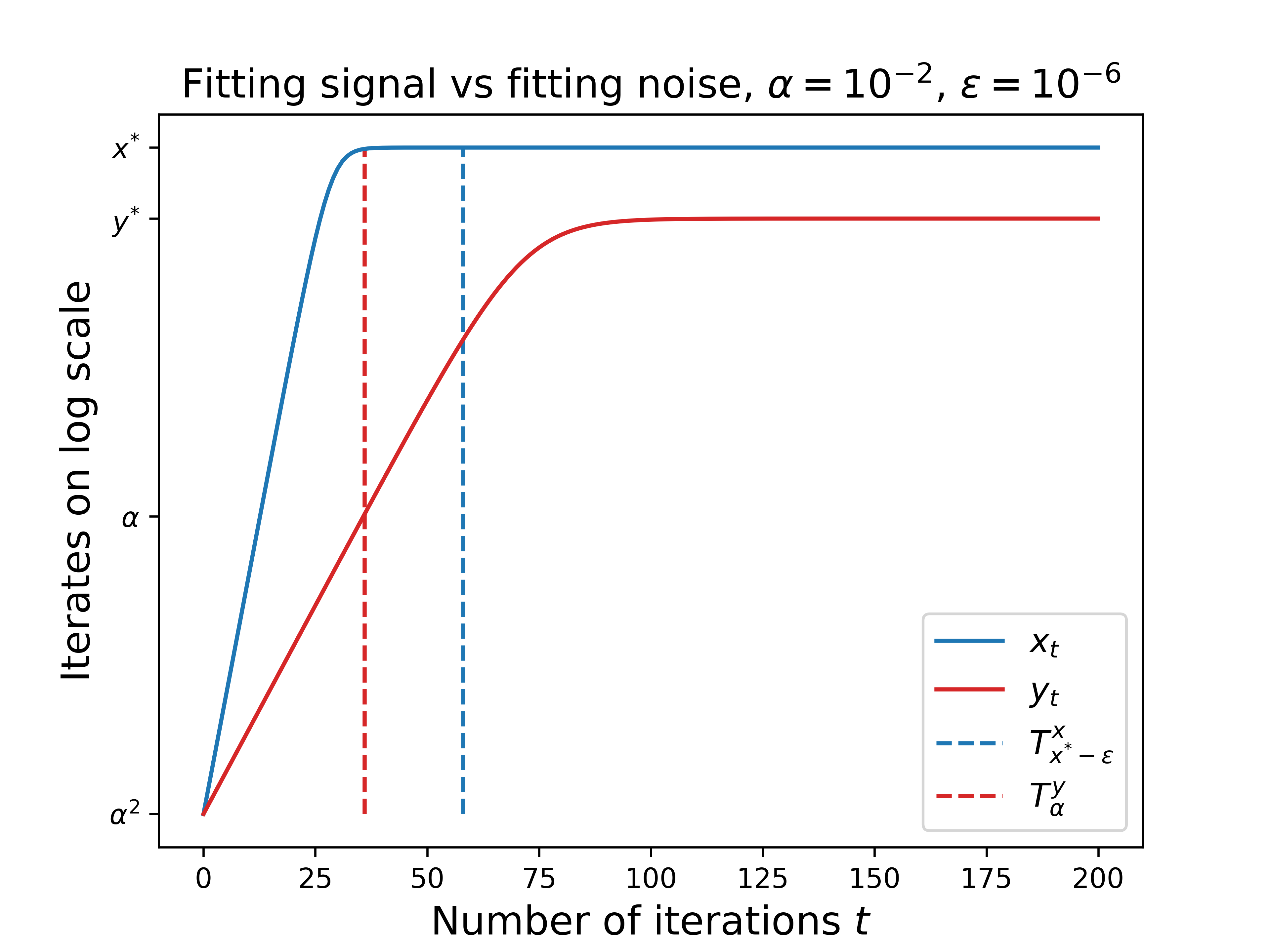
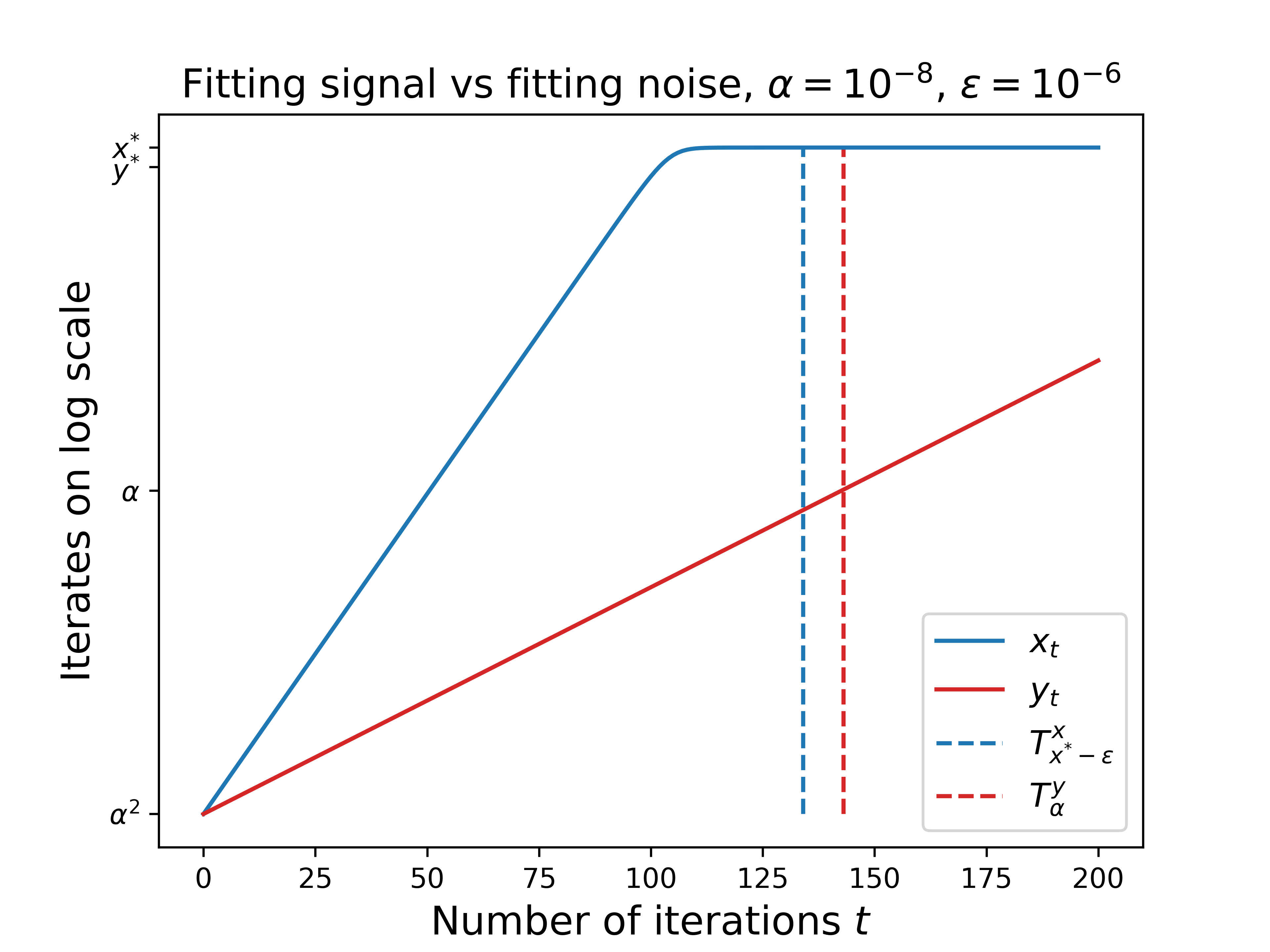
With the above discussion in mind, in this section we will quantitatively formalize under what conditions on $x^{\star},y^{\star},\alpha$ and $\varepsilon$ the inequality $T^{x}_{x^{\star}-\varepsilon}\leq T^{y}_{\alpha}$ hold. We begin by showing that for small enough step sizes, multiplicative update sequences given in equation (5) behave monotonically.

Lemma B.6 (Iterates behave monotonically).

Let $\eta>0$ be the step size and suppose that updates are given by

$$x_{t+1} =x_{t}(1-4\eta(x_{t}-x^{\star}))^{2}.$$

Then the following holds

1. If $0<x_{0}\leq x^{\star}$ and $\eta\leq\frac{1}{8x^{\star}}$ then for any $t>0$ we have $x_{0}\leq x_{t-1}\leq x_{t}\leq x^{\star}$.

2. If $x^{\star}\leq x_{0}\leq\frac{3}{2}x^{\star}$ and $\eta\leq\frac{1}{12x^{\star}}$ then for any $t>0$ we have $x^{\star}\leq x_{t}\leq x_{t-1}\leq x_{0}$.

Proof.

Note that if $x_{0}\leq x_{t}\leq x^{\star}$ then $x_{t}-x^{\star}\leq 0$ and hence $x_{t+1}\geq x_{t}$. Thus for the first part it is enough to show that for all $t\geq 0$ we have $x_{t}\leq x^{\star}$.

Assume for a contradiction that exists $t$ such that

$$x_{0}\leq x_{t}\leq x^{\star},$$

$$x_{t+1}>x^{\star}.$$

Plugging in the update rule for $x_{t+1}$ we can rewrite the above as

$$x_{t} \leq x^{\star}$$

$$<x_{t}(1-4\eta(x_{t}-x^{\star}))^{2}$$

$$\leq x_{t}\left(1+\frac{1}{2}-\frac{x_{t}}{2x^{\star}}\right)^{2}$$

Letting $\lambda\coloneqq\frac{x_{t}}{x^{\star}}$ we then have by our assumption above $0<\lambda\leq 1$. The above inequality then gives us

$$\sqrt{\frac{1}{\lambda}}<3/2-\frac{1}{2}\lambda$$

And hence for $0<\lambda\leq 1$ we have $f(\lambda)\coloneqq\sqrt{\frac{1}{\lambda}}+\frac{1}{2}\lambda<3/2$. Since for $0<\lambda<1$ we also have $f^{\prime}(\lambda)=\frac{1}{2}(1-\frac{1}{\lambda^{3/2}})<0$ and so $f(\lambda)\geq f(1)=3/2$. This gives us the desired contradiction and concludes our proof for the first part.

We will now prove the send part. Similarly to the first part, we just need to show that for all $t\geq 0$ we have $x_{t}\geq x^{\star}$. Suppose that $\frac{3}{2}x^{\star}\geq x_{t}\geq x^{\star}$ and hence we can write $x_{t}=x^{\star}(1+\gamma)$ for some $\gamma\in[0,\frac{1}{2}]$. Then we have

$$x_{t+1} =(1+\gamma)x^{\star}(1-4\eta\gamma x^{\star})^{2}$$

$$\geq(1+\gamma)x^{\star}(1-\frac{1}{3}\gamma)^{2}.$$

One may verify that the polynomial $(1+\gamma)(1-\frac{1}{3}\gamma)^{2}$ is no smaller than one for $0\leq\gamma\leq\frac{1}{2}$ which finishes the second part of our proof. ∎

While the above lemma tells us that for small enough step sizes the iterates are monotonic and bounded, the following two lemmas tell us that we are converging to the target exponentially fast. We first look at the behavior near convergence.

Lemma B.7 (Iterates behaviour near convergence).

Consider the setting of Lemma B.6. Let $x^{\star}>0$ and and suppose that $\left\lvert x_{0}-x^{\star}\right\rvert\leq\frac{1}{2}x^{\star}$. Then the following holds.

1. If $0<x_{0}\leq x^{\star}$ and $\eta\leq\frac{1}{8x^{\star}}$ then for any $t\geq\frac{1}{4\eta x^{\star}}$ we have

   $$0\leq x^{\star}-x_{t}\leq\frac{1}{2}\left\lvert x_{0}-x^{\star}\right\rvert.$$

2. If $x^{\star}\leq x_{0}\leq\frac{3}{2}x^{\star}$ and $\eta\leq\frac{1}{12x^{\star}}$ then for any $t\geq\frac{1}{8\eta x^{\star}}$ we have

   $$0\leq x_{t}-x^{\star}\leq\frac{1}{2}\left\lvert x_{0}-x^{\star}\right\rvert.$$

Proof.

Let us write $\left\lvert x_{0}-x^{\star}\right\rvert=\gamma x^{\star}$ where $\gamma\in[0,\frac{1}{2}]$.

For the first part we have $x_{0}=(1-\gamma)x^{\star}$. Note that while $x_{t}\leq(1-\frac{\gamma}{2})x^{\star}$ we have $x_{t+1}\geq x_{t}(1+4\eta\frac{\gamma}{2}x^{\star})$. Recall that by the Lemma B.6 for all $t\geq 0$ we have $x_{t}\leq x^{\star}$. Hence to find $t$ such that $x^{\star}\geq x_{t}\geq(1-\frac{\gamma}{2})x^{\star}$ it is enough to find a big enough $t$ satisfying the following inequality

$$x_{0}(1+2\eta\gamma x^{\star})^{2t}\geq\left(1-\frac{\gamma}{2}\right)x^{\star}.$$

Noting that for $x>0$ ant $t\geq 1$ we have $(1+x)^{t}\geq 1+tx$ we have

$$x_{0}(1+2\eta\gamma x^{\star})^{2t} \geq x_{0}(1+4\eta\gamma x^{\star}t)$$

and hence it is enough to find a big enough $t$ satisfying

$$x_{0}(1+4\eta\gamma x^{\star}t)\geq\left(1-\frac{\gamma}{2}\right)x^{\star}$$

$$\iff 4\eta\gamma x^{\star}t\geq\frac{\left(1-\frac{\gamma}{2}\right)x^{\star}-x_{0}}{x_{0}}$$

$$\iff 4\eta\gamma x^{\star}t\geq\frac{\gamma}{2(1-\gamma)}$$

$$\iff t\geq\frac{1}{8\eta x^{\star}}\frac{1}{(1-\gamma)}$$

and since $\gamma\in[0,\frac{1}{2}]$ choosing $t\geq\frac{1}{4\eta x^{\star}}$ is enough.

To deal with the second part, now let us write $x_{0}=x^{\star}(1+\gamma)$. We will use a similar approach to the one used in the first part. If for some $x_{t}$ we have $x_{t}\leq(1+\frac{\gamma}{2})x^{\star}$ by Lemma B.6 we would be done. If $x_{t}>x^{\star}(1+\frac{\gamma}{2})$ we have $x_{t+1}\leq x_{t}(1-4\eta\frac{\gamma}{2}x^{\star})^{2}$. This can happen for at most $\frac{1}{8\eta x^{\star}}$ iterations, since

$$x_{0}(1-2\eta\gamma x^{\star})^{2t}\leq x^{\star}(1+\frac{\gamma}{2})$$

$$\iff 2t\log(1-2\eta\gamma x^{\star})\leq\log\frac{x^{\star}(1+\frac{\gamma}{2})}{x^{0}}$$

$$\iff t\geq\frac{1}{2}\frac{\log\frac{x^{\star}(1+\frac{\gamma}{2})}{x^{0}}}{\log(1-2\eta\gamma x^{\star})}.$$

We can deal with the term on the right hand side by noting that

$$\frac{1}{2}\frac{\log\frac{x^{\star}(1+\frac{\gamma}{2})}{x^{0}}}{\log(1-2\eta\gamma x^{\star})} =\frac{1}{2}\frac{\log\frac{1+\frac{\gamma}{2}}{1+\gamma}}{\log(1-2\eta\gamma x^{\star})}$$

$$\leq\frac{1}{2}\frac{\left(\frac{1+\frac{\gamma}{2}}{1+\gamma}-1\right)/\left(\frac{1+\frac{\gamma}{2}}{1+\gamma}\right)}{-2\eta\gamma x^{\star}}$$

$$=\frac{1}{2}\frac{-\frac{\gamma}{2}/\left(1+\frac{\gamma}{2}\right)}{-2\eta\gamma x^{\star}}$$

$$\leq\frac{1}{8\eta x^{\star}}.$$

where in the second line we have used $\log x\leq x-1$ and $\log x\geq\frac{x-1}{x}$. Note, however, that in the above inequalities both logarithms are negative, which is why the inequality signs are reversed. ∎

Lemma B.8 (Iterates approach target exponentially fast).

Consider the setting of updates as in Lemma B.6 and fix any $\varepsilon>0$.

1. If $\varepsilon<\left\lvert x^{\star}-x_{0}\right\rvert\leq\frac{1}{2}x^{\star}$ and $\eta\leq\frac{1}{12x^{\star}}$ then for any $t\geq\frac{3}{8\eta x^{\star}}\log\frac{\left\lvert x^{\star}-x_{0}\right\rvert}{\varepsilon}$ we have

   $$\left\lvert x^{\star}-x_{t}\right\rvert\leq\varepsilon.$$

2. If $0<x_{0}\leq\frac{1}{2}x^{\star}$ and $\eta\leq\frac{1}{8x^{\star}}$ then for any $t\geq\frac{3}{8\eta x^{\star}}\log\frac{(x^{\star})^{2}}{4x_{0}\varepsilon}$ we have

   $$x^{\star}-\varepsilon\leq x_{t}\leq x^{\star}.$$

Proof.

1. To prove the first part we simply need to apply Lemma B.7 $\left\lceil\log_{2}\frac{\left\lvert x^{\star}-x_{0}\right\rvert}{\varepsilon}\right\rceil$ times. Hence after

   $$\frac{\log_{2}e}{4\eta x^{\star}}\log\frac{\left\lvert x^{\star}-x_{0}\right\rvert}{\varepsilon}\leq\frac{3}{8\eta x^{\star}}\log\frac{\left\lvert x^{\star}-x_{0}\right\rvert}{\varepsilon}$$

   iterations we are done.

2. We first need to find a lower-bound on time $t$ which ensures that $x_{t}\geq\frac{x^{\star}}{2}$. Note that while $x_{t}<\frac{x^{\star}}{2}$ we have $x_{t+1}\geq x_{t}(1+2\eta x^{\star})^{2}$. Hence it is enough to choose a big enough $t$ such that

   $$x_{0}(1+2\eta x^{\star})^{2t}\geq\frac{x^{\star}}{2}$$

   $$\iff t\geq\frac{1}{2}\frac{\log\frac{x^{\star}}{2x_{0}}}{\log(1+2\eta x^{\star})}.$$

   We can upper-bound the term on the right by using $\log x\geq\frac{x-1}{x}$ as follows

   $$\frac{1}{2}\frac{\log\frac{x^{\star}}{2x^{\star}}}{\log(1+2\eta x^{\star})} \leq\frac{1}{2}\frac{1+2\eta x^{\star}}{2\eta x_{0}}\log\frac{x^{\star}}{2x_{0}}$$

   $$\leq\frac{5}{16\eta x^{\star}}\log\frac{x^{\star}}{2x_{0}}$$

   and so after $t\geq\frac{5}{16\eta x^{\star}}\log\frac{x^{\star}}{2x_{0}}$ we have $x_{t}\geq\frac{x^{\star}}{2}$.

   Now we can apply the first part to finish the proof. The total sufficient number of iterations is then

   $$\frac{5}{16\eta x^{\star}}\log\frac{x^{\star}}{2x_{0}}+\frac{3}{8\eta x^{\star}}\log\frac{x^{\star}}{2\varepsilon} \leq\frac{3}{8\eta x^{\star}}\log\frac{x^{\star}}{2x_{0}}+\frac{3}{8\eta x^{\star}}\log\frac{x^{\star}}{2\varepsilon}$$

   $$=\frac{3}{8\eta x^{\star}}\log\frac{(x^{\star})^{2}}{4x_{0}\varepsilon}.$$

∎

We are now able to answer the question that we set out at the beginning of this section. That is, under what conditions on $x^{\star},y^{\star},\alpha$ and $\varepsilon$ does the inequality $T^{x}_{x^{\star}-\varepsilon}\leq T^{y}_{\alpha}$ hold? Let $\eta\leq\frac{1}{8x^{\star}}$ and suppose that $x^{\star}\geq 12y^{\star}>0$. Lemmas B.6 and  B.8 then tell us, that for any $\varepsilon>0$ and any

$$t\geq\frac{12}{32\eta x^{\star}}\log\frac{(x^{\star})^{2}}{\alpha^{2}\varepsilon}$$

the sequence $x_{t}$ has converged up to precision $\varepsilon$. Hence

$$T^{x}_{x^{\star}-\varepsilon}\leq\frac{12}{32\eta x^{\star}}\log\frac{(x^{\star})^{2}}{\alpha^{2}\varepsilon}$$ (6)

On the other hand, we can now apply Lemma A.2 to see that for any

$$t\leq\frac{12}{32\eta x^{\star}}\log\frac{1}{\alpha^{4}}\leq\frac{1}{32\eta y^{\star}}\log\frac{1}{\alpha^{4}}$$

we have $y_{t}\leq\alpha$ and hence

$$T^{y}_{\alpha}\geq\frac{12}{32\eta x^{\star}}\log\frac{1}{\alpha^{4}}$$ (7)

We can now see from equations (6) and (7) that it is enough to set $\alpha\leq\frac{\sqrt{\varepsilon}}{x^{\star}}$ so that $T^{x}_{x^{\star}-\varepsilon}\leq T^{y}_{\alpha}$ is satisfied which answers our question.

B.2 Dealing With Bounded Errors

In Section B.1 we analyzed one dimensional multiplicative update sequences and proved that it is possible to fit large enough signal while fitting a controlled amount of error. In this section we extend the setting considered in Section B.1 to handle bounded error sequences $(\mathbf{b}_{t})_{t\geq 0}$ such that for any $t\geq 0$ we have $\left\lVert\mathbf{b}_{t}\right\rVert_{\infty}\leq B$ for some $B\in\mathbb{R}$. That is, we look at one-dimensional multiplicative sequences with positive target $x^{\star}$ with updates given by

$$x_{t+1}=x_{t}(1-4\eta(x_{t}-x^{\star}+b_{t}))^{2}.$$ (8)

Surely, if $B\geq x^{\star}$ one could always set $b_{t}=x^{\star}$ so that the sequence given with the above updates equation shrinks to $0$ and convergence to $x^{\star}$ is not possible. Hence for a given $x^{\star}$ our lemmas below will require $B$ to be small enough, with a particular choice $B\leq\frac{1}{5}x^{\star}$. For a given $B$ one can only expect the sequence $(x_{t})_{t\geq 0}$ to converge to $x^{\star}$ up to precision $B$. To see that, consider two extreme scenarios, one where for all $t\geq 0$ we have $b_{t}=B$ and another with $b_{t}=-B$. This gives rise the following two sequences with updates given by

$$\begin{split}x_{t+1}^{-}&=x_{t}^{-}(1-4\eta(x_{t}^{-}-(x^{\star}-B)))^{2},\\ x_{t+1}^{+}&=x_{t}^{+}(1-4\eta(x_{t}^{-}-(x^{\star}+B)))^{2}.\end{split}$$ (9)

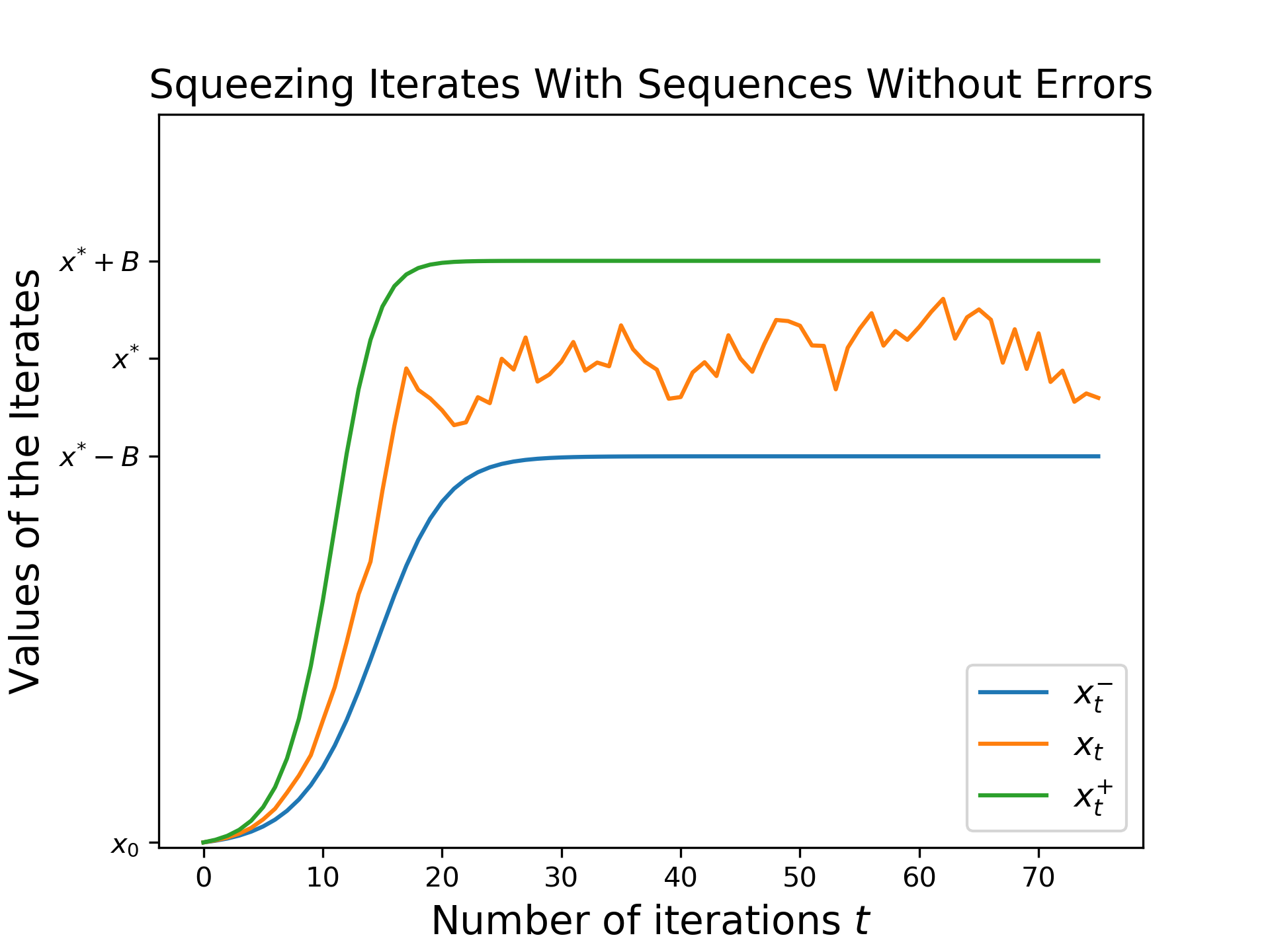
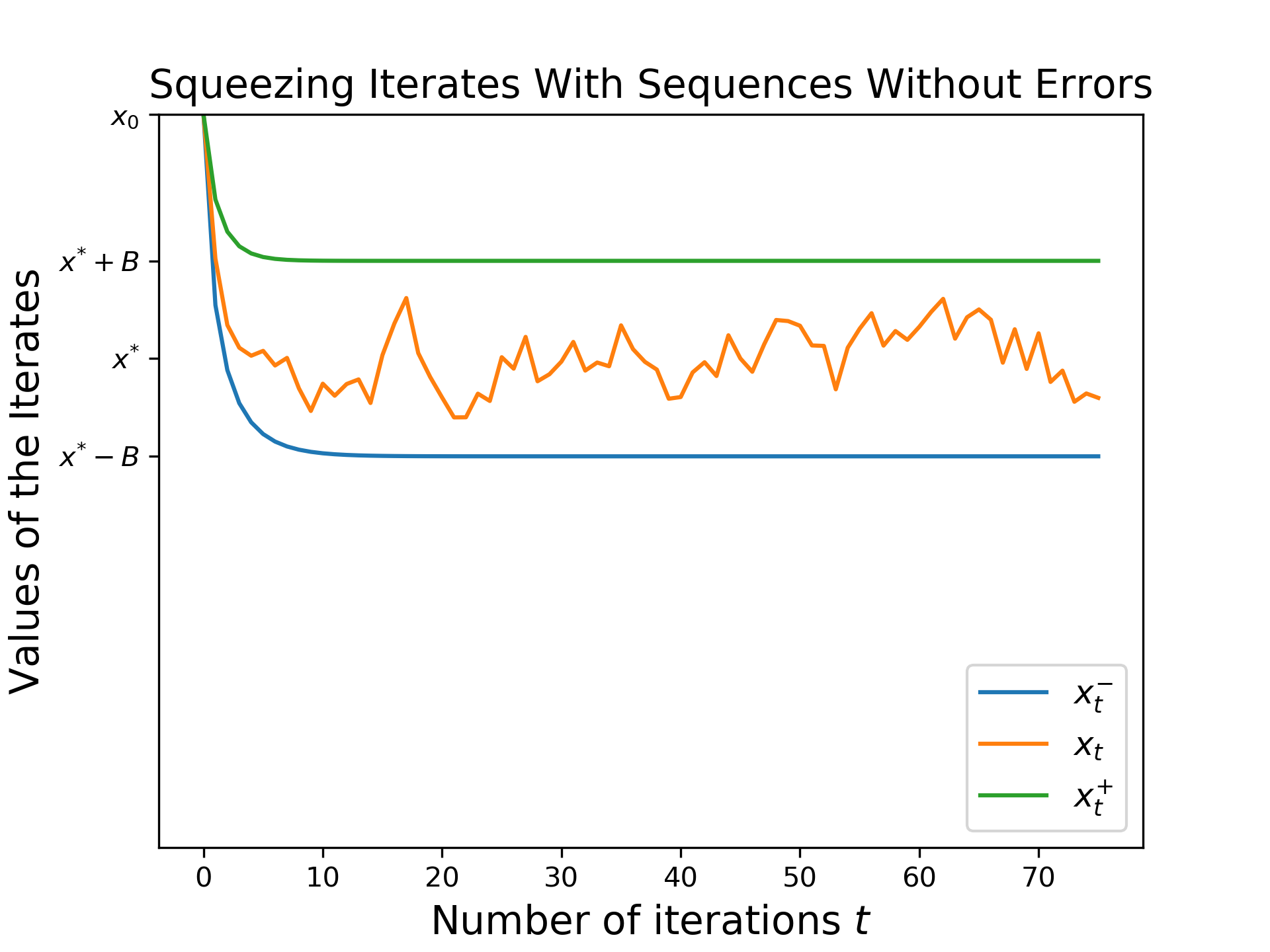
We can think of sequences $(x_{t}^{-})_{t\geq 0}$ and $(x_{t}^{+})_{t\geq 0}$ as sequences with no errors and targets $x^{\star}-B$ and $x^{\star}+B$ respectively. We already understand the behavior of such sequences with the lemmas derived in Section B.1. The following lemma is the key result in this section. It tells us that the sequence $(x_{t})_{t\geq 0}$ is sandwiched between sequences $(x_{t}^{-})_{t\geq 0}$ and $(x_{t}^{+})_{t\geq 0}$ for all iterations $t$. See Figure 8 for a graphical illustration.

Figure 8: A graphical illustration of Lemmas B.9 and B.10. For a given error bound $B$ we have sampled error sequence $(b_{t})_{t\geq 0}$ from $\text{Uniform}[-B,B]$ distribution. Note that for $B=0$ the above plots illustrate Lemma B.6.

Lemma B.9 (Squeezing iterates with bounded errors).

Let $(b_{t})_{t\geq 0}$ be a sequence of errors such that exists some $B>0$ such that for all $t\geq 0$ we have $\left\lvert b_{t}\right\rvert\leq B$. Consider the sequences $(x_{t}^{-})_{t\geq 0}$, $(x_{t})_{t\geq 0}$ and $(x_{t}^{+})_{t\geq 0}$ as defined in equations (8) and (9) with

$$0<x_{0}^{-}=x_{0}^{+}=x_{0}\leq x^{\star}+B$$

If $\eta\leq\frac{1}{16(x^{\star}+B)}$ then for all $t\geq 0$

$$0\leq x_{t}^{-}\leq x_{t}\leq x_{t}^{+}\leq x^{\star}+B.$$

Proof.

We will prove the claim by induction. The claim holds trivially for $t=0$. Then if $x_{t}^{+}\geq x_{t}$, denoting $\Delta\coloneqq x_{t}^{+}-x_{t}\geq 0$ and $m_{t}\coloneqq 1-4\eta(x_{t}-x^{\star}+b_{t})$ we have

$$x_{t+1}^{+} =x_{t}^{+}(1-4\eta(x_{t}^{+}-x^{\star}-B))^{2}$$

$$=(x_{t}+\Delta)(1-4\eta(x_{t}-x^{\star}+b_{t})-4\eta(\Delta-B-b_{t}))^{2}$$

$$\geq(x_{t}+\Delta)(m_{t}-4\eta\Delta)^{2}$$

$$=(x_{t}+\Delta)(m_{t}^{2}-8\eta\Delta m_{t}+16\eta^{2}\Delta^{2})$$

$$\geq(x_{t}+\Delta)(m_{t}^{2}-8\eta\Delta m_{t})$$

$$=x_{t+1}+\Delta m_{t}^{2}-x_{t}^{+}8\eta\Delta m_{t}$$

$$=x_{t+1}+\Delta m_{t}(m_{t}-8\eta x_{t}^{+})$$

$$\geq x_{t+1},$$

where the last line is true since by lemma B.6 we have $0<x_{t}^{+}\leq x^{\star}+B$ and so using $\eta\leq\frac{1}{16(x^{\star}+B)}$ we get

$$m_{t}-8\eta x_{t}^{+} \geq m_{t}-\frac{1}{2}$$

$$=\frac{1}{2}-4\eta(x_{t}-x^{\star}+b_{t})$$

$$\geq\frac{1}{2}-4\eta(x^{\star}+B-x^{\star}+b_{t})$$

$$\geq\frac{1}{2}-8\eta B$$

$$\geq 0.$$

Showing that $x_{t+1}\geq x_{t+1}^{-}$ follows a similar argument.

Finally, as we have already pointed out $x_{t}^{+}\leq x^{\star}+B$ holds for all $t$ by the choice of $\eta$ and Lemma B.6. By induction and the choice of the step size we then also have for all $t\geq 0$

$$x_{t+1}^{-} =x_{t}^{-}(1-4\eta(x_{t}^{-}-x^{\star}+B))^{2}$$

$$\geq x_{t}^{-}(1-8\eta B)^{2}$$

$$\geq 0,$$

which completes our proof. ∎

Using the above lemma we can show analogous results for iterates with bounded errors to the ones shown in Lemmas B.6, B.7 and B.8.

We will first prove a counterpart to Lemma B.6, which is a crucial result in proving Proposition 1. As illustrated in Figure 8, monotonicity will hold while $\left\lvert x_{t}-x^{\star}\right\rvert>B$. On the other hand, once $x_{t}$ hits the $B$-tube around $x^{\star}$ it will always stay inside the tube. This is formalized in the next lemma.

Lemma B.10 (Iterates with bounded errors monotonic behaviour).

Consider the setting of Lemma B.9 with $B\leq\frac{1}{5}x^{\star}$, $\eta\leq\frac{5}{96x^{\star}}$ and $0<x_{0}\leq\frac{6}{5}x^{\star}$. Then the following holds:

1. If $\left\lvert x_{t}-x^{\star}\right\rvert>B$ then $\left\lvert x_{t+1}-x^{\star}\right\rvert<\left\lvert x_{t}-x^{\star}\right\rvert$.

2. If $\left\lvert x_{t}-x^{\star}\right\rvert\leq B$ then $\left\lvert x_{t+1}-x^{\star}\right\rvert\leq B$.

Proof.

First, note that our choice of step size, maximum error $B$ and maximum value for $x_{0}$ ensures that we can apply the second part of Lemma B.6 to the sequence $(x_{t}^{-})_{t\geq 0}$ and the first part of Lemma B.6 to the sequence $(x_{t}^{+})_{t\geq 0}$.

To prove the first part, note that if $0<x_{t}<x^{\star}-B$ then $x_{t}<x_{t+1}\leq x_{t+1}^{+}\leq x^{\star}+B$ and the result follows. On the other hand, if $x^{\star}+B<x_{t}\leq\frac{6}{5}x^{\star}$ then applying Lemma B.9 (with a slight abuse of notation, setting $x_{0}\coloneqq x_{t}$) we get $x^{\star}-B\leq x_{t+1}^{-}\leq x_{t+1}<x_{t}$ which finishes the proof of the first part.

The second part is immediate by Lemma B.9 applied again with a slight abuse of notation setting $x_{0}\coloneqq x_{t}$ and observing that by monotonicity Lemma B.6 the sequence $(x_{t}^{-})_{t\geq 0}$ will monotonically decrease to $x^{\star}-B$ and the sequence $(x_{t}^{+})_{t\geq 0}$ will monotonically increase to $x^{\star}+B$. ∎

Lemma B.11 (Iterates with bounded errors behaviour near convergence).

Consider the setting of Lemma B.10. Then the following holds:

1. If $\frac{1}{2}\left(x^{\star}-B\right)\leq x_{0}\leq x^{\star}-5B$ then for any $t\geq\frac{5}{8\eta x^{\star}}$ we have

   $$\left\lvert x^{\star}-x_{t}\right\rvert\leq\frac{1}{2}\left\lvert x_{0}-x^{\star}\right\rvert.$$

2. If $x^{\star}+4B<x_{0}<\frac{6}{5}x^{\star}$ then for any $t\geq\frac{1}{4\eta x^{\star}}$ we have

   $$\left\lvert x^{\star}-x_{t}\right\rvert\leq\frac{1}{2}\left\lvert x_{0}-x^{\star}\right\rvert.$$

Proof.

Let the sequences $(x_{t}^{+})_{t\geq 0}$ and $(x_{t}^{-})_{t\geq 0}$ be given as in Lemma B.9. For the first part, we apply Lemma B.7 to the sequence $x_{t}^{-}$ twice, to get that for all

$$t\geq\frac{5}{8\eta x^{\star}}\geq 2\frac{1}{4\eta(x^{\star}-B)}$$

we have

$$0 \leq(x^{\star}-B)-x_{t}^{-}$$

$$\leq\frac{1}{4}\left\lvert x_{0}-(x^{\star}-B)\right\rvert$$

$$\leq\frac{1}{4}\left\lvert x_{0}-x^{\star}\right\rvert+\frac{1}{4}B.$$

Then, if $x_{t}\leq x^{\star}$ we have by Lemma B.9 and the above inequality

$$0 \leq x^{\star}-x_{t}$$

$$\leq x^{\star}-x_{t}^{-}$$

$$\leq\frac{1}{4}\left\lvert x_{0}-x^{\star}\right\rvert+\frac{5}{4}B$$

$$\leq\frac{1}{2}\left\lvert x_{0}-x^{\star}\right\rvert.$$

If $x_{t}\geq x^{\star}$ then by lemma B.9 we have

$$0\leq x_{t}-x^{\star}\leq B\leq\frac{1}{5}\left\lvert x_{0}-x^{\star}\right\rvert,$$

where the last inequality follows from $x_{0}\leq x^{*}-5B$. This concludes the first part.

The second part can be shown similarly. We apply lemma B.7 to the sequence $x_{t}^{+}$ twice, to get that for all

$$t\geq 2\frac{1}{8\eta x^{\star}}\geq 2\frac{1}{8\eta(x^{\star}+B)}$$

we have

$$0 \leq x_{t}^{+}-(x^{\star}+B)$$

$$\leq\frac{1}{4}\left\lvert x_{0}-(x^{\star}+B)\right\rvert$$

$$\leq\frac{1}{4}\left\lvert x_{0}-x^{\star}\right\rvert+\frac{1}{4}B.$$

Then again, if $x_{t}\geq x^{\star}$ then

$$0 \leq x_{t}-x^{\star}$$

$$\leq x_{t}^{+}-x^{\star}$$

$$\leq\frac{1}{4}\left\lvert x_{0}-x^{\star}\right\rvert+\frac{5}{4}B$$

$$\leq\frac{1}{2}\left\lvert x_{0}-x^{\star}\right\rvert$$

and if $x_{t}\leq x^{\star}$ then by lemma B.9 we have

$$0\leq x^{\star}-x_{t}\leq B\leq\frac{1}{4}\left\lvert x_{0}-x^{\star}\right\rvert$$

which finishes our proof. ∎

Lemma B.12 (Iterates with bounded errors approach target exponentially fast).

Consider the setting of Lemma B.10 and fix any $\varepsilon>0$. Then the following holds:

1. If $B+\varepsilon<\left\lvert x^{\star}-x_{0}\right\rvert\leq\frac{1}{5}x^{\star}$ then for any $t\geq\frac{15}{32\eta x^{\star}}\log\frac{\left\lvert x^{\star}-x_{0}\right\rvert}{\varepsilon}$ iterations we have $\left\lvert x^{\star}-x_{t}\right\rvert\leq B+\varepsilon$.

2. If $0<x_{0}\leq x^{\star}-B-\varepsilon$ then for any $t\geq\frac{15}{32\eta x^{\star}}\log\frac{(x^{\star})^{2}}{x_{0}\varepsilon}$ we have $x^{\star}-B-\varepsilon\leq x_{t}\leq x^{\star}+B$.

Proof.

1. If $x_{0}>x^{\star}+B$ then by Lemmas B.9 and B.10 we only need show that $(x_{t}^{+})_{t\geq 0}$ hits $x^{\star}+B+\varepsilon$ within the desired number of iterations. By the first part of Lemma B.8 applied to the sequence $(x_{t}^{+})_{t\geq 0}$ we see that $\frac{3}{8\eta(x^{\star}+B)}\log\frac{\left\lvert x_{0}-(x^{\star}+B)\right\rvert}{\varepsilon}\leq\frac{15}{32\eta x^{\star}}\log\frac{\left\lvert x^{\star}-x_{0}\right\rvert}{\varepsilon}$ iterations enough.

   Similarly, if $x_{0}<x^{\star}-B$ by the first part of Lemma B.8 applied to the sequence $(x_{t}^{-})_{t\geq 0}$ we see that $\frac{3}{8\eta(x^{\star}-B)}\log\frac{\left\lvert x_{0}-(x^{\star}-B)\right\rvert}{\varepsilon}\leq\frac{15}{32\eta x^{\star}}\log\frac{\left\lvert x^{\star}-x_{0}\right\rvert}{\varepsilon}$ iterations enough.

2. The upper-bound is immediate from lemma B.9. To get the lower-bound we simply apply the second part of lemma B.8 to the sequence $(x_{t}^{-})_{t\geq 0}$ given in lemma B.9 to get that for any

   $$t\geq\frac{3}{8\eta\frac{4}{5}x^{\star}}\log\frac{(x^{\star})^{2}}{x_{0}\varepsilon}\geq\frac{3}{8\eta(x^{\star}-B)}\log\frac{(x^{\star}-B)^{2}}{x_{0}\varepsilon}$$

   we have $x^{\star}-B-\varepsilon\leq x_{t}^{-}\leq x_{t}$ which is what we wanted to show.

∎

B.3 Dealing With Errors Proportional to Convergence Distance

In this section we derive lemmas helping to deal with errors proportional to convergence distance, that is, the error sequence $(\mathbf{p}_{t})_{t\geq 0}$ given in equation (3) in Appendix A.1. Note that we cannot simply upper-bound $\left\lVert\mathbf{b}_{t}\right\rVert_{\infty}+\left\lVert\mathbf{p}_{t}\right\rVert_{\infty}$ by some large number independent of $t$ and treat both errors together as a bounded error sequence since $\left\lVert\mathbf{p}_{0}\right\rVert_{\infty}$ can be much larger than some of the coordinates of $\mathbf{w}^{\star}$. On the other hand, by Sections B.1 and B.2 we expect $\left\lVert\mathbf{s}_{t}-\mathbf{w}^{\star}\right\rVert_{\infty}$ to decay exponentially fast and hence the error $\left\lVert\mathbf{p}_{t}\right\rVert_{\infty}$ should also decay exponentially fast.

Let $m$ and $T_{0},\dots,T_{m-1}$ be some integers and suppose that we run gradient descent for $\sum_{i=0}^{m-1}T_{i}$ iterations. Suppose that for each time interval $\sum_{i=0}^{j-1}T_{i}\leq t\leq\sum_{i=0}^{j}T_{i}$ we can upper-bound $\left\lVert\mathbf{b}_{t}\right\rVert_{\infty}+\left\lVert\mathbf{p}_{t}\right\rVert_{\infty}$ by $2^{-j}B$ for some $B\in\mathbb{R}$. The following lemma then shows how to control errors of such type and it is, in fact, the reason why in the main theorems a logarithmic term appears in the upper-bounds for the RIP parameter $\delta$. We once again restrict ourselves to one-dimensional sequences.

Lemma B.13 (Halving errors over doubling time intervals).

Let $T>0$ be some fixed positive real number, $T_{i}\coloneqq 2^{i}T$ and $\bar{T_{i}}\coloneqq\sum_{j=0}^{i}T_{j}$. Further, suppose $(p_{t})_{t\geq 0}$ is a sequence of real numbers and let $B\in\mathbb{R}$. Suppose that for every integer $i\geq 0$ and for any $\bar{T}_{i-1}\leq t<\bar{T}_{i}$ we have $\left\lvert p_{t}\right\rvert\leq 2^{-i}B$. Then, for any integer $i\geq 0$ and $\eta\leq\frac{1}{4B}$

$$\prod_{i=0}^{\bar{T}_{i}-1}(1+4\eta p_{t})^{2}\leq(1+4\eta 2^{-i}B)^{2(i+1)T_{i}}.$$

Proof.

Note that for $x,y\geq 0$ we have $(1+x+y)\leq(1+x)(1+y)$ and in particular, for any integers $i\geq j\geq 0$

$$1+4\eta 2^{-j}B\leq(1+4\eta 2^{-j-1}B)^{2}\leq\dots\leq(1+4\eta 2^{-i}B)^{2^{i-j}}.$$

It follows that

$$\prod_{t=0}^{\bar{T}_{i}-1}(1+4\eta p_{t})^{2} \leq\prod_{j=0}^{i}(1+4\eta 2^{-j}B)^{2T_{j}}$$

$$\leq\prod_{j=0}^{i}(1+4\eta 2^{-i}B)^{2^{i-j}2T_{j}}$$

$$=(1+4\eta 2^{-i}B)^{2(i+1)T_{i}}.$$

∎

Sometimes $\left\lVert\mathbf{p}_{t}\right\rVert_{\infty}$ can be much larger than some coordinates of the true parameter vector $\mathbf{w}^{\star}$. For example, if $w^{\star}_{\max}\gg w^{\star}_{\min}$ then $\left\lVert\mathbf{p}_{0}\right\rVert_{\infty}$ can be much larger than $w^{\star}_{\min}$. In Section B.2 we have shown how to deal with bounded errors that are much smaller than target. We now show how to deal with errors much larger than the target.

Lemma B.14 (Handling large errors).

Let $(b_{t})_{t\geq 0}$ be a sequence of errors such that for some $B\in\mathbb{R}$ and all $t\geq 0$ we have $\left\lvert b_{t}\right\rvert\leq B$. Consider a sequence defined as

$$x^{\star}+2B \leq x_{0}\leq x^{\star}+4B,$$

$$x_{t+1} =x_{t}(1-4\eta(x_{t}-x^{\star}+b_{t}))^{2}.$$

Then, for $\eta\leq\frac{1}{20B}$ and any $t\geq\frac{1}{10\eta B}$ we have

$$0\leq x_{t}\leq x^{\star}+2B.$$

Proof.

Note that if $x_{t}\geq x^{\star}+2B$ then

$$x_{t+1} =x_{t}(1-4\eta(x_{t}-x^{\star}+b_{t}))^{2}$$

$$\leq x_{t}(1-4\eta B)^{2}.$$

Hence to find $t$ such that $x_{t}\leq x^{\star}+2B$ it is enough to satisfy the following inequality

$$(x^{\star}+4B)(1-4\eta B)^{2t}\leq x^{\star}+2B$$

$$\iff t\geq\frac{1}{2}\frac{1}{\log(1-4\eta B)}\log\frac{x^{\star}+2B}{x^{\star}+4B}$$

Since for any $x\in(0,1)$ we have $\log(1-x)\leq-x$ hence $\log(1-4\eta B)\leq-4\eta B$. Also, since $\frac{x^{\star}+2B}{x^{\star}+4B}\geq\frac{1}{2}$ we have $\log\frac{x^{\star}+2B}{x^{\star}+4B}\geq\log\frac{1}{2}\geq-\frac{7}{10}$. Hence

$$\frac{1}{2}\frac{1}{\log(1-4\eta B)}\log\frac{x^{\star}+2B}{x^{\star}+4B}\leq\frac{1}{2}\cdot\frac{1}{-4\eta B}\cdot\frac{-7}{10}.$$

Setting $t\geq\frac{1}{10\eta B}$ is hence enough. To ensure non-negativity of the iterates, note that

$$\left\lvert 4\eta(x_{t}-x^{\star}+b_{t})\right\rvert\leq 20\eta B$$

and hence setting $\eta\leq\frac{1}{20B}$ is enough. ∎

The final challenge caused by the error sequence $(\mathbf{p}_{t})_{t\geq 0}$ is that some of the signal components $\mathbf{1}_{S}\odot\mathbf{w}_{t}$ can actually shrink initially instead of approaching the target. Hence for all $t\geq 0$ we need to control the maximum shrinkage by bounding the following term from below

$$\alpha^{2}\prod_{i=0}^{t-1}(1-4\eta(\left\lVert\mathbf{b}_{t}\right\rVert_{\infty}+\left\lVert\mathbf{p}_{t}\right\rVert_{\infty}))^{2}.$$ (10)

Recall that we are handling maximum growth of the error sequence $(\mathbf{e}_{t})_{t\geq 0}$ by Lemma A.1 which requires upper-bounding the term

$$\alpha^{2}\prod_{i=0}^{t-1}(1+4\eta(\left\lVert\mathbf{b}_{t}\right\rVert_{\infty}+\left\lVert\mathbf{p}_{t}\right\rVert_{\infty}))^{2}.$$ (11)

If the term in equation (11) is not too large, then we can prove that the term in equation (10) cannot be too small. This idea is exploited in the following lemma.

Lemma B.15 (Handling signal shrinkage).

Consider a sequence

$$x_{0} =\alpha^{2},$$

$$x_{t+1} =x_{t}(1-4\eta(x^{\star}+b_{t}+p_{t}))^{2}$$

where $x^{\star}>0$ and exists some $B>0$ such that for all $t\geq 0$ we have $\left\lvert b_{t}\right\rvert+\left\lvert p_{t}\right\rvert\leq B$. If $\eta\leq\frac{1}{8B}$ and

$$\prod_{i=0}^{t-1}(1+8\eta(\left\lvert b_{t}\right\rvert+\left\lvert p_{t}\right\rvert))^{2}\leq\frac{1}{\alpha}$$

then

$$\prod_{i=0}^{t-1}(1-4\eta(\left\lvert b_{t}\right\rvert+\left\lvert p_{t}\right\rvert))^{2}\geq\alpha.$$

Proof.

By the choice of step size $\eta$ we always have $0\leq 4\eta(\left\lvert b_{t}\right\rvert+\left\lvert p_{t}\right\rvert)\leq\frac{1}{2}$. Since for $x\in[0,\frac{1}{2}]$ we have $(1+2x)(1-x)=1+x-2x^{2}\geq 1$ it follows that

$$\prod_{i=0}^{t-1}(1+8\eta(\left\lvert b_{t}\right\rvert+\left\lvert p_{t}\right\rvert))^{2}\prod_{i=0}^{t-1}(1-4\eta(\left\lvert b_{t}\right\rvert+\left\lvert p_{t}\right\rvert))^{2}\geq 1$$

and we are done. ∎

B.4 Dealing With Negative Targets

So far we have only dealt with sequences converging to some positive target, i.e., the parametrization $\mathbf{w}_{t}=\mathbf{u}_{t}\odot\mathbf{u}_{t}$. In this section we show that handling parametrization $\mathbf{w}_{t}=\mathbf{u}_{t}\odot\mathbf{u}_{t}-\mathbf{v}_{t}\odot\mathbf{v}_{t}$ can be done by noting that for any coordinate $i$, at least one of $u_{t,i}$ or $v_{t,i}$ has to be close to its initialization value. Intuitively, this observation will allow us to treat parametrization $\mathbf{w}_{t}=\mathbf{u}_{t}\odot\mathbf{u}_{t}-\mathbf{v}_{t}\odot\mathbf{v}_{t}$ as if it was $\mathbf{w}_{t}\approx\mathbf{u}_{t}\odot\mathbf{u}_{t}$ and all coordinates of the target $\mathbf{w}^{\star}$ are replaced by its absolute values.

Consider two sequences given by

$$0<x^{+}_{0} =\alpha^{2}\leq x^{\star}_{+},\quad x^{+}_{t+1}=x^{+}_{t}(1-4\eta(x^{+}_{t}-x^{\star}_{+}+b_{t}))^{2}$$

$$0<x^{-}_{0} =\alpha^{2}\leq-x^{\star}_{-},\quad x_{t+1}^{-}=x^{-}_{t}(1+4\eta(-x^{-}_{t}-x_{-}^{\star}+b_{t}))^{2}$$

where $(b_{t})_{t\geq 0}$ is some sequence of errors and the targets satisfy $x_{+}^{\star}>0$ and $x_{-}^{\star}<0$. We already know how to deal with the sequence $(x^{+}_{t})_{t\geq 0}$. Note that we can rewrite the updates for the sequence $(x^{-}_{t})_{t\geq 0}$ as follows

$$x^{-}_{t+1}=x^{-}_{t}(1-4\eta(x^{-}_{t}-\left\lvert x_{-}^{\star}\right\rvert-b_{t}))^{2}.$$

and we know how to deal with sequences of this form. In particular, $(x^{-}_{t})_{t\geq 0}$ will converge to $\left\lvert x_{-}^{\star}\right\rvert$ with error at most $B$ equal to some bound on maximum error and hence the sequence $(-x^{-}_{t})_{t\geq 0}$ will converge to a $B$-tube around $x^{\star}$. Hence, our theory developed for sequences with positive targets directly apply for sequences with negative targets of the form given above.

The following lemma is the key result allowing to treat $\mathbf{w}_{t}=\mathbf{u}_{t}\odot\mathbf{u}_{t}-\mathbf{v}_{t}\odot\mathbf{v}_{t}$ almost as if it was $\mathbf{w}_{t}\approx\mathbf{u}_{t}\odot\mathbf{u}_{t}$ as discussed at the beginning of this section.

Lemma B.16 (Handling positive and negative sequences simultaneously).

Let $x_{t}=x_{t}^{+}-x^{-}_{t}$ and $x^{\star}\in\mathbb{R}$ be the target such that $\left\lvert x^{\star}\right\rvert>0$. Suppose the sequences $(x^{+}_{t})_{t\geq 0}$ and $(x^{-}_{t})_{t\geq 0}$ evolve as follows

$$0<x^{+}_{0}=\alpha^{2}\leq\frac{1}{4}\left\lvert x^{\star}\right\rvert,\quad x^{+}_{t+1}=x^{+}_{t}(1-4\eta(x_{t}-x^{\star}+b_{t}))^{2}$$

$$0<x^{-}_{0}=\alpha^{2}\leq\frac{1}{4}\left\lvert x^{\star}\right\rvert,\quad x^{-}_{t+1}=x^{-}_{t}(1+4\eta(x_{t}-x^{\star}+b_{t}))^{2}.$$

and that there exists $B>0$ such that $\left\lvert b_{t}\right\rvert\leq B$ and $\eta\leq\frac{1}{12(x^{\star}+B)}$. Then the following holds:

1. For any $t\geq 0$ we have $0\leq x^{+}_{t}\wedge x^{-}_{t}\leq\alpha^{2}$.

2. For any $t\geq 0$ we have

   • If $x^{\star}>0$ then $x^{-}_{t}\leq\alpha^{2}\prod_{i=0}^{t-1}(1+4\eta\left\lvert b_{t}\right\rvert)$.

   • If $x^{\star}<0$ then $x^{+}_{t}\leq\alpha^{2}\prod_{i=0}^{t-1}(1+4\eta\left\lvert b_{t}\right\rvert)$.

Proof.

The choice of our step size ensures that $\left\lvert 4\eta(x_{t}-x^{\star}+b_{t})\right\rvert\leq\frac{1}{2}$. For any $0\leq a\leq\frac{1}{2}$ we have $0\leq(1-a)(1+a)=1-a^{2}\leq 1$. In particular, this yields for any $t\geq 0$

$$x^{+}_{t}x^{-}_{t}=\alpha^{4}\prod_{i=0}^{t-1}(1-4\eta(x_{t}-x^{\star}+b_{t}))^{2}(1+4\eta(x_{t}-x^{\star}+b_{t}))^{2}\leq\alpha^{4}$$

which concludes the first part.

To prove the second part assume $x^{\star}>0$ and fix any $t\geq 0$. Let $0\leq s\leq t$ be the largest $s$ such that $x^{+}_{s}>x^{\star}$. If no such $s$ exists we are done immediately. If $s=t$ then by the first part we have $x^{-}_{t}\leq\alpha^{2}$ and we are done.

If $s<t$ then we have by the first part and by the assumption $\alpha^{2}\leq\frac{1}{4}\left\lvert x^{\star}\right\rvert$,  $x^{-}_{s}\leq\frac{\alpha^{4}}{x^{+}_{s}}\leq\frac{1}{4}\alpha^{2}$. Further, by the choice of step size $\eta$ we have $x^{+}_{s}\leq 4x^{\star}$. It then follows that

$$(1+4\eta(x_{s}-x^{\star}+b_{t}))^{2}\leq 4$$

and hence

$$x^{-}_{t} =x^{-}_{s}\prod_{i=s}^{t-1}(1+4\eta(x^{+}_{i}-x^{-}_{i}-x^{\star}+b_{i}))^{2}$$

$$\leq\frac{1}{4}\alpha^{2}(1+4\eta(x_{s}-x^{\star}+b_{t}))^{2}\prod_{i=s+1}^{t-1}(1+4\eta(x^{+}_{i}-x^{-}_{i}-x^{\star}+b_{i}))^{2}$$

$$\leq\alpha^{2}\prod_{i=s+1}^{t-1}(1+4\eta\left\lvert b_{t}\right\rvert))^{2}.$$

This completes our proof for the case $x^{\star}>0$. For $x^{\star}<0$ we are done by symmetry. ∎

B.5 Proof of Proposition 1

In this section we will prove Proposition 1. We remind our readers, that the goal of this proposition is showing that the error sequence $(\mathbf{p}_{t})_{t\geq 0}$ can be essentially ignored if the RIP constant $\delta$ is small enough.

Recall that the error arising due to the bounded error sequence $(\mathbf{b}_{t})_{t\geq 0}$ is irreducible as discussed in Section B.2. More formally, we will show that if for some $0\leq\zeta\leq w^{\star}_{\max}$ we have $\left\lVert\mathbf{b}_{t}\right\rVert_{\infty}\lesssim\zeta$ and if $\left\lVert\mathbf{p}_{t}\right\rVert_{\infty}\lesssim\frac{1}{\log_{2}\frac{w^{\star}_{\max}}{\zeta}}\left\lVert s_{t}-\mathbf{w}^{\star}\right\rVert_{\infty}$ then after $t=O\left(\frac{1}{\eta\zeta}\log\frac{1}{\alpha}\right)$ iterations we have $\left\lVert\mathbf{s}_{t}-\mathbf{w}^{\star}\right\rVert_{\infty}\leq\zeta$. In particular, up to absolute multiplicative constants we perform as good as if the error sequence $(\mathbf{p}_{t})_{t\geq 0}$ was equal to $0$.

The proof idea is simple, but the details can complicated. We will first prove a counterpart to Proposition 1 which will correspond to parametrization $\mathbf{w}_{t}=\mathbf{u}_{t}\odot\mathbf{u}_{t}$, that is, we will only try to fit the positive coordinates of $\mathbf{w}^{\star}$. We will later use Lemma B.16 to extend our result to the general case. We now list the key ideas appearing in the proof below.

1. Initially we have $\left\lVert\mathbf{w}_{0}-\mathbf{w}^{\star}\right\rVert_{\infty}\leq w^{\star}_{\max}$. We will prove our claim by induction, reducing the above distance by half during each induction hypothesis. We will hence need to apply $m\coloneqq\left\lceil\log_{2}\frac{w^{\star}_{\max}}{\zeta}\right\rceil$ induction steps which we will enumerated from $0$ to $m-1$.

2. At the beginning of the $i^{\mathit{th}}$ induction step we will have $\left\lVert\mathbf{w}_{t}-\mathbf{w}^{\star}\right\rVert_{\infty}\leq 2^{-i}w^{\star}_{\max}$. Choosing small enough absolute constants for upper-bounds on error sequences $(\mathbf{b}_{t})_{t\geq 0}$ and $(\mathbf{p}_{t})_{t\geq 0}$ we can show that

   $$\left\lVert\mathbf{b}_{t}\right\rVert_{\infty}+\left\lVert\mathbf{p}_{t}\right\rVert_{\infty}\leq\frac{1}{40}2^{-i}w^{\star}_{\max}\eqqcolon B_{i}.$$

   In particular, during the $i^{\mathit{th}}$ induction step we treat both types of errors simultaneously as a bounded error sequence with bound $B_{i}$. Since at each induction step $\left\lVert\mathbf{w}_{t}-\mathbf{w}^{\star}\right\rVert_{\infty}$ decreases by half, the error bound $B_{i}$ also halves. This puts us in position to apply Lemma B.13 which plays a key role in the proof below.

3. One technical difficulty is that in Section B.2 all lemmas require that iterates never exceed the target by more than a factor $\frac{6}{5}$. We cannot ensure that since initially our errors can be much larger than some of the true parameter $\mathbf{w}^{\star}$ coordinates. We instead use Lemma B.14 to show that for any coordinate $j$ we have $w_{t,j}\leq w_{j}^{\star}+4B_{i}$ during $i^{\mathit{th}}$ induction step. Then for any $j$ such that $w_{j}^{\star}\geq 20B_{i}$ we can apply the results from Section B.2. On the other hand, if $w_{j}^{\star}\leq 20B_{i}=\frac{1}{2}2^{-i}w^{\star}_{\max}$ then we already have $\left\lvert w_{t,j}-w^{\star}_{j}\right\rvert\leq 2^{-i-1}w^{\star}_{\max}$ and the above bound does not change during the $i^{\mathit{th}}$ induction step.

4. During the $i^{\mathit{th}}$ induction step, if $\left\lvert w_{t,j}-w^{\star}_{j}\right\rvert>2^{-i-1}w^{\star}_{\max}$ then $w_{j}^{\star}\geq 20B_{i}$ and we can apply Lemma B.10 which says that all such coordinates will monotonically approach $B$-tube around $w^{\star}_{j}$. Lemma B.12 then tells us how many iterations need to be taken for our iterates to get close enough to this $B$-tube so that $\left\lvert w_{t,j}-w^{\star}_{j}\right\rvert\leq 2^{-i-1}w^{\star}_{\max}$.

5. Finally, we control the total accumulation of errors $\prod_{i=0}^{t-1}(1+4\eta(\left\lVert\mathbf{b}_{i}\right\rVert_{\infty}+\left\lVert\mathbf{p}_{i}\right\rVert_{\infty}))^{2}$ using Lemma B.13 and ensure that for any $w_{j}^{\star}\geq 0$ the iterates never get below $\alpha^{3}$ by applying Lemma B.15.

Lemma B.17 (Dealing with errors proportional to convergence distance).

Fix any $0<\zeta\leq w^{\star}_{\max}$ and let $\gamma=\frac{C_{\gamma}}{\lceil\log_{2}\frac{w^{\star}_{\max}}{\zeta}\rceil}$ where $C_{\gamma}$ is some small enough absolute constant. Let $\mathbf{w}^{\star}\in\mathbb{R}^{k}$ be a target vector which is now allowed to have negative components. Denote by $\mathbf{w}^{\star}_{+}$ the positive part of $\mathbf{w}^{\star}$, that is, $(w^{\star}_{+})_{i}=\mathbb{1}_{\{w^{\star}_{i}\geq 0\}}w^{\star}_{i}$. Let $(\mathbf{b}_{t})_{t\geq 0}$ and $(\mathbf{p}_{t})_{t\geq 0}$ sequences of errors such that for all $t\geq 0$ we have $\left\lVert\mathbf{b}_{t}\right\rVert_{\infty}\leq C_{b}\zeta$ for some small enough absolute constant $C_{b}$ and $\left\lVert\mathbf{p}_{t}\right\rVert_{\infty}\leq\gamma\left\lVert\mathbf{w}_{t}-\mathbf{w}^{\star}_{+}\right\rVert_{\infty}$. Let the updates be given by

$$w_{0,j}=\alpha^{2},\quad w_{t+1,j}=w_{t,j}(1-4\eta(w_{t,j}-w^{\star}_{j}+b_{t,j}+p_{t,j}))^{2}.$$

If the step size satisfies $\eta\leq\frac{5}{96w^{\star}_{\max}}$ and the initialization satisfies $\alpha\leq\frac{\zeta}{3(w^{\star}_{\max})^{2}}\wedge\sqrt{w^{\star}_{\min}}\wedge 1$ then for $t=O\left(\frac{1}{\eta\zeta}\log\frac{1}{\alpha}\right)$ we have

$$\left\lVert\mathbf{w}_{t}-\mathbf{w}^{\star}_{+}\right\rVert_{\infty} \leq\zeta$$

$$\alpha^{2}\prod_{i=0}^{t-1}(1+4\eta(\left\lVert\mathbf{b}_{t}\right\rVert_{\infty}+\left\lVert\mathbf{p}_{t}\right\rVert_{\infty}))^{2} \leq\alpha.$$

Proof.

Let $T\coloneqq\frac{1}{\eta w^{\star}_{\max}}\log\frac{1}{\alpha^{4}}$ and for any integer $i\geq-1$ let $T_{i}\coloneqq 2^{i}T$ and $\bar{T}_{i}\coloneqq\sum_{j=0}^{i}T_{j}$. We also let $\bar{T}_{-1}=0$. Let $B_{i}\coloneqq\frac{1}{40}2^{-i}w^{\star}_{\max}$. Let $m=\left\lceil\log_{2}\frac{w^{\star}_{\max}}{\zeta}\right\rceil$ so that $\gamma=\frac{C_{\gamma}}{m}$. We will prove our claim by induction on $i=0,1,\dots,m-1$.

Induction hypothesis for $i\in\{0,\dots,m\}$

1. For any $j<i$ and $\bar{T}_{j-1}\leq t<\bar{T}_{j}$ we have $\left\lVert\mathbf{w}_{t}-\mathbf{w}^{\star}_{+}\right\rVert_{\infty}\leq 2^{-j}w^{\star}_{\max}$. In particular, this induction hypothesis says that we halve the convergence distance during each induction step.

2. We have $\left\lVert\mathbf{w}_{\bar{T}_{i-1}}-\mathbf{w}^{\star}_{+}\right\rVert_{\infty}\leq 2^{-i}w^{\star}_{\max}$. This hypothesis controls the convergence distance at the beginning of the $i^{\mathit{th}}$ induction step.

3. For any $j$ we have $\alpha^{3}\leq w_{\bar{T}_{i-1},j}\leq w_{j}^{\star}+4B_{i}$.

Base case
For $i=0$ all conditions hold since for all $j$ we have $0\leq\alpha^{2}=w_{0,j}<w^{\star}_{j}$.

Induction step
Assume that the induction hypothesis holds for some $0\leq i<m$. We will show that it holds for $i+1$.

1. We want to show that for all $t\in\{0,\dots,T_{i}-1\}$ $\left\lVert\mathbf{w}_{\bar{T}_{i-1}+t}-\mathbf{w}^{\star}_{+}\right\rVert_{\infty}$ remains upper-bounded by $2^{-i}w^{\star}_{\max}$.

   Note that $2^{-i}w^{\star}_{\max}\geq 2^{-m}w^{\star}_{\max}\geq\frac{1}{2}\zeta$ and hence requiring $C_{\gamma}+2C_{b}\leq\frac{1}{40}$ we have

   $$\left\lVert\mathbf{b}_{\bar{T}_{i-1}}\right\rVert_{\infty}+\left\lVert\mathbf{p}_{\bar{T}_{i-1}}\right\rVert_{\infty} \leq C_{b}\zeta+\gamma 2^{-i}w^{\star}_{\max}$$

   $$\leq(C_{\gamma}+2C_{b})2^{-i}w^{\star}_{\max}$$

   $$\leq\frac{1}{40}2^{-i}w^{\star}_{\max}$$

   $$=B_{i}.$$

   For any $j$ such that $w_{j}^{\star}\geq 20B_{i}$ the third induction hypothesis $w_{\bar{T}_{i-1},j}\leq w_{j}^{\star}+4B_{i}$ ensures that $w_{\bar{T}_{i-1},j}\leq\frac{6}{5}w_{j}^{\star}$. Hence, it satisfies the pre-conditions of Lemma B.10 and as long as

   $$\left\lVert\mathbf{w}_{\bar{T}_{i-1}+t}-\mathbf{w}^{\star}_{+}\right\rVert_{\infty}\leq 2^{-i}w^{\star}_{\max}$$

   any such $j$ will monotonically approach the $\frac{1}{40}B_{i}$-tube around $w_{j}^{\star}$ maintaining $\left\lvert w_{t}-w_{j}^{\star}\right\rvert\leq 2^{-i}w^{\star}_{\max}$.

   On the other hand, for any $j$ such that $w_{j}^{\star}\leq 20B_{i}$ $w_{t,j}$ will stay in $(0,w_{j}^{\star}+4B_{i}]$ maintaining $\left\lvert w_{t}-w_{j}^{\star}\right\rvert\leq 20B_{i}\leq 2^{-i}w^{\star}_{\max}$ as required.

   By induction on $t$, we then have for any $t\geq 0$

   $$\left\lVert\mathbf{w}_{\bar{T}_{i-1}+t}-\mathbf{w}^{\star}_{+}\right\rVert_{\infty}\leq 2^{-i}w^{\star}_{\max}$$

   which is what we wanted to show.

2. To prove the second part of the induction hypothesis, we need to show that after $T_{i}$ iterations the maximum convergence distance $\left\lVert\mathbf{w}_{\bar{T}_{i}}-\mathbf{w}^{\star}_{+}\right\rVert_{\infty}$ decreases at least by half.

   Take any $j$ such that $w^{\star}_{j}\geq 0$ and $\left\lvert w_{\bar{T}_{i-1},j}^{\star}-w^{\star}_{j}\right\rvert\leq 2^{-i-1}w^{\star}_{\max}=20B_{i}$. Then by a similar argument used in to prove the first induction hypothesis for any $t\geq 0$ we have $\left\lvert w_{\bar{T}_{i-1}+t,j}^{\star}-w^{\star}_{j}\right\rvert\leq 2^{-i-1}w^{\star}_{\max}$ and hence such coordinates can be ignored.

   Now take any $j$ such that $w^{\star}_{j}\geq 0$ and $\left\lvert w_{\bar{T}_{i-1},j}^{\star}-w^{\star}_{j}\right\rvert>2^{-i-1}w^{\star}_{\max}$. Then, since $20B_{i}=2^{-i-1}w^{\star}_{\max}$ and since by the third induction hypothesis $w_{\bar{T}_{i-1},j}\leq w^{\star}_{j}+4B_{i}$ it follows that $0\leq w_{\bar{T}_{i-1},j}<w^{\star}_{j}-20B_{i}$. Applying the second part of Lemma B.12 with $\varepsilon=19B_{i}$ and noting that

   $$19B_{i}=\frac{19}{40}2^{-i}w^{\star}_{\max}\geq\frac{19}{40}2^{-m+1}w^{\star}_{\max}\geq\frac{19}{40}\zeta\geq\frac{1}{3}\zeta$$

   we have for any

   $$t \geq T_{i}$$

   $$\geq 2^{i}\frac{1}{\eta w^{\star}_{\max}}\log\frac{3(w^{\star}_{\max})^{2}}{\alpha^{3}\zeta}$$

   $$\geq\frac{15}{32\eta w_{j}^{\star}}\log\frac{(w_{j}^{\star})^{2}}{w_{\bar{T}_{i-1},j}\cdot 19B_{i}}$$

   iterations the following holds

   $$\left\lvert w_{\bar{T}_{i-1}+t,j}-w^{\star}_{j}\right\rvert\leq 20B_{i}\leq 2^{-i-1}w^{\star}_{\max}$$

   which completes our proof.

3. The upper bound follows immediately from Lemma B.14 which tells that after

   $$t\geq T_{i}\geq 2^{i}\frac{4}{\eta w^{\star}_{\max}}=\frac{1}{10\eta B_{i}}.$$

   iterations for any $j$ we have $w_{\bar{T}_{i-1}+t,j}\leq w^{\star}_{j}+2B_{i}=w^{\star}_{j}+4B_{i+1}$.

   To prove the lower-bound, first note that

   $$\prod_{i=0}^{\bar{T}_{i}-1}(1+8\eta(\left\lVert\mathbf{b}_{i}\right\rVert_{\infty}+\left\lVert\mathbf{p}_{i}\right\rVert_{\infty}))^{2}$$

   $$\leq\prod_{i=0}^{\bar{T}_{i}-1}(1+8\eta C_{b}\zeta)^{2}(1+4\eta\left\lVert\mathbf{p}_{i}\right\rVert_{\infty}))^{4}$$ (12)

   $$\leq(1+8\eta C_{b}\zeta)^{4T_{i}}\left(1+4\eta\cdot\frac{C_{\gamma}}{m}2^{-i}w^{\star}_{\max}\right)^{4(i+1)T_{i}}$$ (13)

   $$\leq(1+8\eta C_{b}\zeta)^{4T_{m-1}}\left(1+4\eta\cdot\frac{C_{\gamma}}{m}2^{-m+1}w^{\star}_{\max}\right)^{4mT_{m-1}}$$ (14)

   $$\leq\left(1+4\eta\cdot\frac{1}{m}2C_{b}\zeta\right)^{4mT_{m-1}}\left(1+4\eta\cdot\frac{C_{\gamma}}{m}2^{-m+1}w^{\star}_{\max}\right)^{4mT_{m-1}}$$ (15)

   $$\leq\left(1+4\eta\cdot\frac{C_{\gamma}}{m}2^{-m+1}w^{\star}_{\max}\right)^{8mT_{m-1}}$$ (16)

   $$\leq\frac{1}{\alpha}$$ (17)

   where line 12 follows by noting that for any $x,y\geq 0$ we have $(1+x+y)\leq(1+x)(1+y)$. Line 13 follows by applying Lemma B.13 and noting that $\bar{T}_{i}\leq 2T_{i}$. Line 14 follows by noting that $i\leq m-1$. Line 15 follows by applying $(1+mx)\leq(1+x)^{m}$ for $x\geq 0$ and $m\geq 1$. Line 16 follows by noting that $\zeta\leq 2^{-m+1}w^{\star}_{\max}$ and assuming that $2C_{b}\leq C_{\gamma}$. Line 17 follows by applying Lemma A.2 which in particular says that

   $$\left(1+4\eta\cdot\frac{C_{\gamma}}{m}2^{-m+1}w^{\star}_{\max}\right)^{2t}\leq\frac{1}{\alpha}$$

   for any $t\leq\frac{m2^{m-1}}{32\eta w^{\star}_{\max}C_{\gamma}}\log\frac{1}{\alpha^{4}}$. Setting $C_{\gamma}=\frac{1}{128}$ yields the desired result.

   The lower-bound is then proved immediately by Lemma B.15.

By above, the induction hypothesis holds for $i=m$. We can still repeat the argument for the first step of induction hypothesis to show that for any $t\geq\bar{T}_{m-1}$

$$\left\lVert\mathbf{w}_{t}-\mathbf{w}^{\star}_{+}\right\rVert_{\infty}\leq 2^{-m}w^{\star}_{\max}\leq\zeta.$$

Also, the proof for the third induction hypothesis with $i=m$ shows that for any $t\leq\bar{T}_{m-1}$ we have

$$\alpha^{2}\prod_{i=0}^{t-1}(1+4\eta(\left\lVert\mathbf{b}_{t}\right\rVert_{\infty}+\left\lVert\mathbf{p}_{t}\right\rVert_{\infty}))^{2}\leq\alpha.$$

To simplify the presentation, note that $\frac{w^{\star}_{\max}}{\zeta}\leq 2^{m}<\frac{2w^{\star}_{\max}}{\zeta}$ and hence we will write

$$\bar{T}_{m-1}=(2^{m}-1)\frac{1}{\eta w^{\star}_{\max}}\log\frac{1}{\alpha^{4}}=O\left(\frac{1}{\eta\zeta}\log\frac{1}{\alpha}\right).$$

Finally, regarding the absolute constants we have required in our proofs above that $C_{\gamma}+2C_{b}\leq\frac{1}{40}$, $C_{b}\leq\frac{1}{2}C_{\gamma}$ and $C_{\gamma}\leq\frac{1}{128}$. Hence, for example, absolute constants $C_{b}=\frac{1}{256}$ and $C_{\gamma}=\frac{1}{128}$ satisfy the requirements of this lemma. ∎

Extending the above lemma to the general setting considered in Proposition 1 can now be done by a simple application of Lemma B.16 as follows.

Proof of Proposition 1.

Lemma B.16 allows us to reduce this proof to lemma B.17 directly. In particular, using notation from Lemma B.17 and using Lemma B.16 we maintain that for all $t\leq\bar{T}_{m-1}$

$$w^{\star}_{j}>0 \implies 0\leq w^{-}_{t}\leq\alpha$$

$$w^{\star}_{j}<0 \implies 0\leq w^{+}_{t}\leq\alpha.$$

Consequently, for $w^{\star}_{j}>0$ we can ignore sequence $(w_{t,j}^{-})_{t\geq 0}$ by treating it as a part of bounded error $b_{t}$. The same holds for sequence $(w_{t,j}^{+})_{t\geq 0}$ when $w^{\star}_{j}<0$. Then, for $w_{j}^{\star}>0$ the sequence $(w_{t,j}^{+})$ evolves as follows

$$w_{t+1,j}^{+}=w_{t,j}^{+}(1-4\eta(w_{t,j}^{+}-w^{\star}_{j}+(b_{t,j}-w^{-}_{t,j})+p_{t,j}))^{2}$$

which falls directly into the setting of lemma B.17. Similarly, if $w^{\star}_{j}<0$ then

$$w_{t+1,j}^{-} =w_{t,j}^{-}(1+4\eta(-w_{t,j}^{-}-w^{\star}_{j}+(b_{t,j}+w^{+}_{t,j})+p_{t,j}))^{2}$$

$$=w_{t,j}^{-}(1-4\eta(w_{t,j}^{-}-\left\lvert w^{\star}_{j}\right\rvert+(-b_{t,j}-w^{+}_{t,j})-p_{t,j}))^{2}$$

and hence this sequence also falls into the setting of lemma B.17.

Finally, $\left\lVert\mathbf{e}_{t}\right\rVert_{\infty}\leq\alpha$ follows by Lemma A.1 and we are done. ∎

B.6 Proof of Proposition 2

We split the proof of Proposition 2 in two phases. First, using Lemma B.18 we show that $\left\lVert\mathbf{s}_{t}-\mathbf{w}^{\star}\right\rVert_{\infty}$ converges to $0$ with error $\left\lVert\mathbf{b}_{t}\odot\mathbf{1}_{S}\right\rVert_{\infty}$ up to some absolute multiplicative constant. From this point onward, we can apply Lemma B.12 to handle convergence to each individual sequence $i$ on the true support $S$ up to the error $\left\lVert\mathbf{b}_{t}\odot\mathbf{1}_{i}\right\rVert_{\infty}\vee\sqrt{k}\delta\left\lVert\mathbf{b}_{t}\odot\mathbf{1}_{S}\right\rVert_{\infty}$. This is exactly what allows us to approach an oracle-like performance with the $\ell_{2}$ parameter estimation error depending on $\log k$ instead of $\log d$ in the case of sub-Gaussian noise.

Lemma B.18.

Consider the setting of updates given in equations (3) and (4). Fix any $\varepsilon>0$ and suppose that the error sequences $(\mathbf{b}_{t})_{t\geq 0}$ and $(\mathbf{p}_{t})_{t\geq 0}$ satisfy the following for any $t\geq 0$:

$$\left\lVert\mathbf{b}_{t}\odot\mathbf{1}_{S}\right\rVert_{\infty} \leq B,$$

$$\left\lVert\mathbf{p}_{t}\right\rVert_{\infty} \leq\frac{1}{20}\left\lVert\mathbf{s}_{t}-\mathbf{w}^{\star}\right\rVert_{\infty}.$$

Suppose that

$$20B<\left\lVert\mathbf{s}_{0}-\mathbf{w}^{\star}\right\rVert_{\infty}\leq\frac{1}{5}w^{\star}_{\min}.$$

Then for $\eta\leq\frac{5}{96w^{\star}_{\max}}$ and any $t\geq\frac{5}{8\eta w^{\star}_{\min}}$ we have

$$\left\lVert\mathbf{s}_{t}-\mathbf{w}^{\star}\right\rVert_{\infty}\leq\frac{1}{2}\left\lVert\mathbf{s}_{0}-\mathbf{w}^{\star}\right\rVert_{\infty}.$$

Proof.

Note that $\left\lVert\mathbf{b}_{0}\right\rVert_{\infty}+\left\lVert\mathbf{p}_{0}\right\rVert_{\infty}\leq\frac{1}{10}\left\lVert\mathbf{s}_{0}-\mathbf{w}^{\star}\right\rVert_{\infty}$. By Lemma B.10 for any $t\geq 0$ we have $\left\lVert\mathbf{b}_{t}\right\rVert_{\infty}+\left\lVert\mathbf{p}_{t}\right\rVert_{\infty}\leq\frac{1}{10}\left\lVert\mathbf{s}_{0}-\mathbf{w}^{\star}\right\rVert_{\infty}$. Hence, for any $i$ such that $\left\lvert s_{0,i}-w^{\star}_{i}\right\rvert\leq\frac{1}{2}\left\lVert\mathbf{s}_{0}-\mathbf{w}^{\star}\right\rVert_{\infty}$ Lemma B.10 guarantees that for any $t\geq 0$ we have $\left\lvert s_{t,i}-w^{\star}_{i}\right\rvert\leq\frac{1}{2}\left\lVert\mathbf{s}_{0}-\mathbf{w}^{\star}\right\rVert_{\infty}$ On the other hand, for any $i$ such that $\left\lvert s_{0,i}-w^{\star}_{i}\right\rvert>\frac{1}{2}\left\lVert\mathbf{s}_{0}-\mathbf{w}^{\star}\right\rVert_{\infty}$ by Lemma B.11 we have $\left\lvert s_{t,i}-w^{\star}_{i}\right\rvert\leq\frac{1}{2}\left\lVert\mathbf{s}_{0}-\mathbf{w}^{\star}\right\rVert_{\infty}$ for any $t\geq\frac{5}{8\eta w^{\star}_{\min}}$ which is what we wanted to prove. ∎

Proof of Proposition 2.

Let $B\coloneqq\max_{j\in S}B_{j}$. To see that $\left\lVert\mathbf{s}_{t}-\mathbf{w}^{\star}\right\rVert_{\infty}$ never exceeds $\frac{1}{5}w^{\star}_{\min}$ we use the $B$-tube argument developed in Section B.2 and formalized in Lemma B.10.

We begin by applying the Lemma B.18 for $\log_{2}\frac{w^{\star}_{\min}}{5(B\vee\varepsilon)}$ times. Now we have $\left\lVert\mathbf{s}_{t}-\mathbf{w}^{\star}\right\rVert_{\infty}<20(B\vee\varepsilon)$ and so $\left\lVert\mathbf{p}_{t}\right\rVert_{\infty}<\delta\sqrt{k}\cdot 20(B\vee\varepsilon)$ Hence, for any $i\in S$ we have

$$\left\lVert\mathbf{b}_{t}\odot\mathbf{1}_{i}\right\rVert_{\infty}+\left\lVert\mathbf{p}_{t}\right\rVert_{\infty}\leq B_{i}+\sqrt{k}\delta 20(B\vee\varepsilon).$$

Hence for each coordinate $i\in S$ we can apply the first part of Lemma B.12 so that after another $t=\frac{15}{32\eta w^{\star}_{\min}}\log\frac{w^{\star}_{\min}}{5\varepsilon}$ iterations we are done.

Hence the total number of required iterations is at most $t\leq\frac{45}{32\eta w^{\star}_{\min}}\log\frac{w^{\star}_{\min}}{\varepsilon}$.

∎

Appendix C Missing Proofs from Section A.3

This section provides proofs for the technical lemmas stated in section A.3.

C.1 Proof of Lemma A.1

Looking at the updates given by equation 4 in appendix A.1 we have

$$\mathbf{1}_{S^{c}}\odot\mathbf{e}_{t+1} =\mathbf{1}_{S^{c}}\odot\mathbf{w}_{t}\odot(\mathbf{1}-4\eta(\mathbf{s}_{t}-\mathbf{w}^{\star}+\mathbf{b}_{t}+\mathbf{p}_{t}))^{2}$$ (18)

$$=\mathbf{1}_{S^{c}}\odot\mathbf{e}_{t}\odot\left(\mathbf{1}_{S^{c}}-\mathbf{1}_{S^{c}}\odot 4\eta(\mathbf{s}_{t}-\mathbf{w}^{\star}+\mathbf{b}_{t}+\mathbf{p}_{t})\right)^{2}$$ (19)

$$=\mathbf{1}_{S^{c}}\odot\mathbf{e}_{t}\odot\left(\mathbf{1}-4\eta(\mathbf{b}_{t}+\mathbf{p}_{t})\right)^{2}$$ (20)

and hence

$$\left\lVert\mathbf{1}_{S^{c}}\odot\mathbf{e}_{t+1}\right\rVert_{\infty} \leq\left\lVert\mathbf{1}_{S^{c}}\odot\mathbf{e}_{t}\right\rVert_{\infty}(1+4\eta(\left\lVert\mathbf{b}_{t}\right\rVert_{\infty}+\left\lVert\mathbf{p}_{t}\right\rVert_{\infty}))^{2}$$

which completes the proof for $\mathbf{1}_{S^{c}}\odot\mathbf{e}_{t}$.

On the other hand, Lemma B.16 deals with $\mathbf{1}_{S}\odot\mathbf{e}_{t}$ immediately and we are done. ∎

C.2 Proof of Lemma A.2

Note that

$$1+4\eta b_{t}\leq 1+4\eta B$$

and hence

$$x_{t}\leq x_{0}(1+4\eta B)^{2t}.$$

To ensure that $x_{t}\leq\sqrt{x_{0}}$ it is enough to ensure that the right hand side of the above expression is not greater than $\sqrt{x_{0}}$. This is satisfied by all $t$ such that

$$t\leq\frac{1}{2}\frac{\log\frac{1}{\sqrt{x_{0}}}}{\log\left(1+4\eta B\right)}$$

Now by using $\log x\leq x-1$ we have

$$\frac{1}{2}\frac{\log\frac{1}{\sqrt{x_{0}}}}{\log\left(1+4\eta B\right)} \geq\frac{1}{2}\frac{\log\frac{1}{\sqrt{x_{0}}}}{4\eta B}$$

$$=\frac{1}{32\eta B}\log\frac{1}{x_{0}^{2}}$$

which concludes our proof. ∎

C.3 Proof of Lemma A.3

For any index set $S$ of size $k+1$ let $\mathbf{X}_{S}$ be the $n\times(k+1)$ sub-matrix of $\mathbf{X}$ containing columns indexed by $S$. Let $\lambda_{\max}\left(\frac{1}{n}\mathbf{X}_{S}^{\mathsf{T}}\mathbf{X}_{S}\right)$ and $\lambda_{\min}\left(\frac{1}{n}\mathbf{X}_{S}^{\mathsf{T}}\mathbf{X}_{S}\right)$ denote the maximum and minimum eigenvalues of $\left(\frac{1}{n}\mathbf{X}_{S}^{\mathsf{T}}\mathbf{X}_{S}\right)$ respectively. It is then a standard consequence of the $(k+1,\delta)$-RIP that

$$1-\delta\leq\lambda_{\min}\left(\frac{1}{n}\mathbf{X}_{S}^{\mathsf{T}}\mathbf{X}_{S}\right)\leq\lambda_{\max}\left(\frac{1}{n}\mathbf{X}_{S}^{\mathsf{T}}\mathbf{X}_{S}\right)\leq 1+\delta.$$

Let $\mathbf{z}\in\mathbb{R}^{d}$ be any $k$-sparse vector. Then, for any $i\in\{1,\dots,d\}$ the joint support of $\mathbf{1}_{i}$ and $\mathbf{z}$ is of size at most $k+1$. We denote the joint support by $S$ and we will also denote by $\mathbf{z}_{S}$ and $(\mathbf{1}_{i})_{S}$ the restrictions of $\mathbf{z}$ and $\mathbf{1}_{i}$ on their support, i.e., vectors in $\mathbb{R}^{k+1}$. Letting $\left\lVert\cdot\right\rVert$ be the spectral norm, we have

$$\left\lvert\left(\frac{1}{n}\mathbf{X}^{\mathsf{T}}\mathbf{X}\mathbf{z}\right)_{i}-\mathbf{z}_{i}\right\rvert =\left\lvert\left\langle\frac{1}{n}\mathbf{X}^{\mathsf{T}}\mathbf{X}\mathbf{z},\mathbf{1}_{i}\right\rangle-\left\langle\mathbf{z},\mathbf{1}_{i}\right\rangle\right\rvert$$

$$=\left\lvert\left\langle\frac{1}{\sqrt{n}}\mathbf{X}\mathbf{z},\frac{1}{\sqrt{n}}\mathbf{X}\mathbf{1}_{i}\right\rangle-\left\langle\mathbf{z},\mathbf{1}_{i}\right\rangle\right\rvert$$

$$=\left\lvert\left\langle\frac{1}{\sqrt{n}}\mathbf{X}_{S}\mathbf{z}_{S},\frac{1}{\sqrt{n}}\mathbf{X}_{S}(\mathbf{1}_{i})_{S}\right\rangle-\left\langle\mathbf{z}_{S},(\mathbf{1}_{i})_{S}\right\rangle\right\rvert$$

$$=\left\lvert\left\langle\left(\frac{1}{n}\mathbf{X}_{S}^{\mathsf{T}}\mathbf{X}_{S}-\mathbf{I}\right)\mathbf{z}_{S},(\mathbf{1}_{i})_{S}\right\rangle\right\rvert$$

$$\leq\left\lVert\frac{1}{n}\mathbf{X}_{S}^{\mathsf{T}}\mathbf{X}_{S}-\mathbf{I}\right\rVert\left\lVert\mathbf{z}\right\rVert_{2}\left\lVert\mathbf{1}_{i}\right\rVert_{2}$$

$$\leq\delta\left\lVert\mathbf{z}\right\rVert_{2}$$

where the penultimate line follows by the Cauchy-Schwarz inequality and the last line follows by the $(k+1,\delta)$-RIP. Since $i$ was arbitrary it hence follows that

$$\left\lVert\left(\frac{1}{n}\mathbf{X}^{\mathsf{T}}\mathbf{X}-\mathbf{I}\right)\mathbf{z}\right\rVert_{\infty}\leq\delta\left\lVert\mathbf{z}\right\rVert_{2}\leq\delta\sqrt{k}\left\lVert\mathbf{z}\right\rVert_{\infty}.$$

∎

C.4 Proof of Lemma A.4

For any $i\in\{1,\dots,d\}$ we can write $\mathbf{X}_{i}=\mathbf{X}\mathbf{1}_{i}$. The result is then immediate by the $(k+1,\delta)$-RIP since

$$\left\lVert\frac{1}{\sqrt{n}}\mathbf{X}\mathbf{1}_{i}\right\rVert_{2}^{2}\leq(1+\delta)\left\lVert\mathbf{1}_{i}\right\rVert_{2}^{2}\leq 2.$$

By the Cauchy-Schwarz inequality we then have, for any $i,j\in\{1,\dots,d\}$,

$$\left\lvert\left(\frac{1}{n}\mathbf{X}^{\mathsf{T}}\mathbf{X}\right)_{i,j}\right\rvert\leq\left\lVert\frac{1}{\sqrt{n}}\mathbf{X}_{i}\right\rVert_{2}\left\lVert\frac{1}{\sqrt{n}}\mathbf{X}_{j}\right\rVert_{2}\leq 2$$

and for any $\mathbf{z}\in\mathbb{R}^{d}$ it follows that

$$\left\lVert\frac{1}{n}\mathbf{X}^{\mathsf{T}}\mathbf{X}\mathbf{z}\right\rVert_{\infty}\leq 2d\left\lVert\mathbf{z}\right\rVert_{\infty}.$$

∎

C.5 Proof of Lemma A.5

Since for any column $\mathbf{X}_{i}$ of the matrix $\mathbf{X}$ we have $\left\lVert X_{i}\right\rVert_{2}/\sqrt{n}\leq C$ and since the vector $\mathbf{\xi}$ consists of independent $\sigma^{2}$-subGaussian random variables, the random variable $\frac{1}{\sqrt{n}}\left(\mathbf{X}^{\mathsf{T}}\mathbf{\xi}\right)_{i}$ is $C^{2}\sigma^{2}$-subGaussian.

It is then a standard result that for any $\varepsilon>0$

$$\mathbb{P}\!\left({\left\lVert\frac{1}{\sqrt{n}}\mathbf{X}^{\mathsf{T}}\mathbf{\xi}\right\rVert_{\infty}>\varepsilon}\right)\leq 2de^{-\frac{\varepsilon^{2}}{2C^{2}\sigma^{2}}}.$$

Setting $\varepsilon=2\sqrt{2C^{2}\sigma^{2}\log(2d)}$ we have with probability at least $1-\frac{1}{8d^{3}}$ we have

$$\left\lVert\frac{1}{\sqrt{n}}\mathbf{X}^{\mathsf{T}}\mathbf{\xi}\right\rVert_{\infty} \leq 4\sqrt{C^{2}\sigma^{2}\log(2d)}$$

$$\lesssim\sqrt{\sigma^{2}\log d}.$$

∎

Appendix D Proof of Theorem 2

Recall the updates equations for our model parameters given in equations (3) and (4) as defined in Appendix A.1.

Since $\mathbf{w}_{0}=0$ we can rewrite the first update written on $\mathbf{u}$ and $\mathbf{v}$ as

$$\begin{split}\mathbf{u}_{1}&=\mathbf{u}_{0}\odot\left(\mathbf{1}-4\eta\left(-\mathbf{w}^{\star}+\left(\mathbf{I}-\frac{1}{n}\mathbf{X}^{\mathsf{T}}\mathbf{X}\right)\mathbf{w}^{\star}-\frac{1}{n}\mathbf{X}^{\mathsf{T}}\xi)\right)\right),\\ \mathbf{v}_{1}&=\mathbf{v}_{0}\odot\left(\mathbf{1}+4\eta\left(-\mathbf{w}^{\star}+\left(\mathbf{I}-\frac{1}{n}\mathbf{X}^{\mathsf{T}}\mathbf{X}\right)\mathbf{w}^{\star}-\frac{1}{n}\mathbf{X}^{\mathsf{T}}\xi)\right)\right).\end{split}$$ (21)

By Lemma A.3 we have $\left\lVert\left(\mathbf{I}-\frac{1}{n}\mathbf{X}^{\mathsf{T}}\mathbf{X}\right)\mathbf{w}^{\star}\right\rVert_{\infty}\leq\frac{1}{20}w^{\star}_{\max}$. The term $\frac{1}{n}\mathbf{X}^{\mathsf{T}}\xi$ can be simply bounded by $\left\lVert\frac{1}{n}\mathbf{X}^{\mathsf{T}}\mathbf{\xi}\right\rVert_{\infty}$. If $w^{\star}_{\max}\geq 5\left\lVert\frac{1}{n}\mathbf{X}^{\mathsf{T}}\mathbf{\xi}\right\rVert_{\infty}$ (note that otherwise returning a $0$ vector is minimax-optimal) then

$$\frac{1}{20}w^{\star}_{\max}+\left\lVert\frac{1}{n}\mathbf{X}^{\mathsf{T}}\mathbf{\xi}\right\rVert_{\infty}\leq\frac{1}{4}w^{\star}_{\max}.$$

We can hence bound the below term appearing in equation (21) as follows:

$$\frac{3}{4}w^{\star}_{\max}\leq\left\lVert-\mathbf{w}^{\star}+\left(\mathbf{I}-\frac{1}{n}\mathbf{X}^{\mathsf{T}}\mathbf{X}\right)\mathbf{w}^{\star}-\frac{1}{n}\mathbf{X}^{\mathsf{T}}\xi)\right\rVert_{\infty}\leq\frac{5}{4}w^{\star}_{\max}$$

The main idea here is that we can recover the above factor by computing one gradient descent iteration and hence we can recover $w^{\star}_{\max}$ up to some multiplicative constants.

In fact, with $0<\eta\leq\frac{1}{5w^{\star}_{\max}}$ so that the multiplicative factors are non-negative, the above inequality implies that

$$1+3\eta w^{\star}_{\max}\leq f_{\max}\leq 1+5\eta w^{\star}_{\max}$$

and so

$$w^{\star}_{\max}\leq\frac{f_{\max}-1}{3\eta}\leq\frac{5}{3}w^{\star}_{\max}$$

which is what we wanted to show.

Note that after an application of this theorem we can now reset the step size to

$$\frac{3\eta}{20\left(f_{\max}-1\right)}.$$

This new step size satisfies the conditions of Theorems 1 and 3 while being at most two times smaller than required.

Appendix E Proof of Theorem 3

For proving Theorem 3 we first prove Propositions 3 and 4 which correspond to Propositions 1 and 2 but allows for different step sizes along each dimension. We present the proof of Proposition 3 in Section E.1.

Proposition 3.

Consider the setting of Proposition 1 and run Algorithm 2 with $\tau=640$.

Then, for some early stopping time $T=O\left(\log{\frac{w^{\star}_{\max}}{\zeta}}\log\frac{1}{\alpha}\right)$ and any $0\leq t\leq T$ we have

$$\left\lVert\mathbf{s}_{T}-\mathbf{w}^{\star}\right\rVert_{\infty} \leq\zeta,$$

$$\left\lVert\mathbf{e}_{t}\right\rVert_{\infty} \leq\alpha.$$

Further, let $\eta_{T,j}$ be the step size for the $j^{\mathit{th}}$ coodinate at time $T$. Then, for all $j$ such that $\lvert w^{\star}_{j}\rvert>\zeta$ we have

$$\frac{1}{16}\cdot\frac{1}{20\left\lvert w^{\star}_{j}\right\rvert}\leq\eta_{T,j}\leq\frac{1}{20\left\lvert w^{\star}_{j}\right\rvert}.$$

Proposition 4.

Consider the setting of updates given in equations (3) and (4). Fix any $\varepsilon>0$ and suppose that the error sequences $(\mathbf{b}_{t})_{t\geq 0}$ and $(\mathbf{p}_{t})_{t\geq 0}$ satisfy for any $t\geq 0$:

$$\left\lVert\mathbf{b}_{t}\odot\mathbf{1}_{i}\right\rVert_{\infty} \leq B_{i}\leq\frac{1}{10}w^{\star}_{\min},$$

$$\left\lVert\mathbf{p}_{t}\right\rVert_{\infty} \leq\frac{1}{20}\left\lVert\mathbf{s}_{t}-\mathbf{w}^{\star}\right\rVert_{\infty}.$$

Suppose that

$$\left\lVert\mathbf{s}_{0}-\mathbf{w}^{\star}\right\rVert_{\infty}\leq\frac{1}{5}w^{\star}_{\min}.$$

For each $i\in S$ let the step size satisfy $\frac{1}{\eta_{i}\left\lvert w^{\star}_{i}\right\rvert}\leq 320$. Then for all $t\geq 0$

$$\left\lVert\mathbf{s}_{t}-\mathbf{w}^{\star}\right\rVert_{\infty}\leq\frac{1}{5}w^{\star}_{\min}$$

and for any $t\geq 450\log\frac{w^{\star}_{\min}}{\varepsilon}$ we have for any $i\in S$.

$$\left\lvert s_{t,i}-w^{\star}_{i}\right\rvert\lesssim\delta\sqrt{k}\max_{j\in S}B_{j}\vee B_{i}\vee\varepsilon$$

Proof.

We follow the same strategy as in the proof of Proposition 2. The only difference here is that the worst case convergence time $\frac{1}{\eta w^{\star}_{\min}}$ is replaced by $\max_{i\in S}\frac{1}{\eta_{i}\left\lvert w^{\star}_{i}\right\rvert}\leq 320$ and the result follows. ∎

Proof of Theorem 3.

The proof is identical to the proof of Theorem 1 with application of Proposition 1 replaced with Proposition 3 and in the easy setting the application of Proposition 2 replaced with an application of Proposition 4.

The only difference is that extra care must be taken when applying Proposition 4. First, note that the pre-conditions on step sizes are satisfied by Proposition 3. Second, the number of iterations required by Proposition 4 is fewer than step-size doubling intervals, and hence the step sizes will not change after the application of Proposition 3. In particular, Proposition 3 requires $450\log\frac{w^{\star}_{\min}}{\varepsilon}$ iterations and we double the step sizes every $640\log\frac{1}{\alpha}$ iterations. This finishes our proof. ∎

E.1 Proof of Proposition 3

Recall the proof of Proposition 1 that we have shown in Appendix B.5. We have used a constant step size $\eta\leq\frac{5}{96w^{\star}_{\max}}$. With a constant step size this is in fact unavoidable up to multiplicative constants – for larger step sizes the iterates can explode.

Looking at our proof by induction of Lemma B.17, the inefficiency of Algorithm 1 comes from doubling the number of iterations during each induction step. This happens because during the $i^{\mathit{th}}$ induction step the smallest coordinates of $\mathbf{w}^{\star}$ that we consider are of size $2^{-i-1}w^{\star}_{\max}$. For such coordinates, step size $\eta\leq\frac{5}{96w^{\star}_{\max}}$ could be at least $2^{i}$ times bigger and hence the convergence would be $2^{i}$ times faster. The lemmas derived in Appendix B.2 indicate that fitting signal of such size will require number of iterations proportional to $\frac{1}{\eta 2^{-i-1}w^{\star}_{\max}}=2^{i+1}\frac{1}{\eta w^{\star}_{\max}}$ which is where the exponential increase in the number of iterations for each induction step comes from.

We can get rid of this inefficiency if for each coordinate $j$ we use a different step size, so that for all $j$ such that $\left\lvert w_{j}^{\star}\right\rvert\ll w^{\star}_{\max}$ we set $\eta_{j}\gg\frac{5}{96w^{\star}_{\max}}$. In fact, the only constraint we have is that $\eta_{j}$ never exceeds $\frac{5}{96\left\lvert w^{\star}\right\rvert_{j}}$. To see that we can change the step sizes for small enough signal in practice, note that after two induction steps in Proposition 1 we have $\left\lVert\mathbf{s}_{t}-\mathbf{w}^{\star}\right\rVert_{\infty}\leq\frac{1}{4}w^{\star}_{\max}$ and $\left\lVert\mathbf{e}_{t}\right\rVert_{\infty}\leq\alpha$. We can then show, that for each $j$ such that $\left\lvert w^{\star}\right\rvert_{j}>\frac{1}{2}w^{\star}_{\max}$ we have $\left\lvert w_{t,j}\right\rvert>\frac{1}{4}w^{\star}_{\max}$. On the other hand, if $\left\lvert w^{\star}\right\rvert_{j}\leq\frac{1}{8}w^{\star}_{\max}$ then $w_{t,j}\leq w^{\star}_{j}+4B_{1}\leq\frac{1}{4}w^{\star}_{\max}$, where $B_{1}$ is given as in Lemma B.17. In particular, after the second induction step one can take all $j$ such that $\left\lvert w_{t,j}\right\rvert\leq\frac{1}{4}w^{\star}_{\max}$ and double its associated step sizes.

We exploit the above idea in the following lemma, which is a counterpart to Lemma B.17. One final thing to note is that we do not really know what $w^{\star}_{\max}$ is which is necessary in the argument sketched above. However, in Theorem 2 we showed that we can compute some $\hat{z}$ such that $w^{\star}_{\max}\leq\hat{z}\leq 2w^{\star}_{\max}$ and as we shall see this is enough.

Lemma E.19 (Counterpart to Lemma B.17 with increasing step sizes).

Consider the same setting of Lemma B.17. Run Algorithm 2 with $\tau=640$ and parametrization $\mathbf{w}_{t}=\mathbf{u}_{t}\odot\mathbf{u}_{t}$.

Then, for $t=\left\lceil 640\log_{2}\frac{w^{\star}_{\max}}{\zeta}\log\frac{1}{\alpha}\right\rceil$ and any $j$ we have

$$\left\lVert\mathbf{w}_{t}-\mathbf{w}^{\star}_{+}\right\rVert_{\infty} \leq\zeta$$

$$\alpha^{2}\prod_{i=0}^{t-1}(1+4\eta_{t,j}(\left\lVert\mathbf{b}_{t}\right\rVert_{\infty}+\left\lVert\mathbf{p}_{t}\right\rVert_{\infty}))^{2} \leq\alpha.$$

Proof.

Following the notation used in Lemma B.17 for any integer $i\geq-1$ let $T_{i}\coloneqq T$ and $\bar{T}_{i}\coloneqq\sum_{j=0}^{i}T_{j}=(i+1)T$. We remark now that we have the same $T$ for each induction step in contrast to exponentially increasing number of iterations in Lemma B.17. Let $B_{i}\coloneqq\frac{1}{40}2^{-i}w^{\star}_{\max}$. Let $m=\left\lceil\log_{2}\frac{w^{\star}_{\max}}{\zeta}\right\rceil$ so that $\gamma=\frac{C_{\gamma}}{m}$. We will prove our claim by induction on $i=0,1,\dots,m-1$.

Induction hypothesis for $i\in\{0,\dots,m\}$

1. For any $j<i$ and $\bar{T}_{j-1}\leq t<\bar{T}_{j}$ we have $\left\lVert\mathbf{w}_{t}-\mathbf{w}^{\star}_{+}\right\rVert_{\infty}\leq 2^{-j}w^{\star}_{\max}$. In particular, this induction hypothesis says that we halve the convergence distance during each induction step.

2. We have $\left\lVert\mathbf{w}_{\bar{T}_{i-1}}-\mathbf{w}^{\star}_{+}\right\rVert_{\infty}\leq 2^{-i}w^{\star}_{\max}$. This hypothesis controls the convergence distance at the beginning of each induction step.

3. For any $j$ such that $w^{\star}_{j}\leq 20B_{i}=2^{-i-1}w^{\star}_{\max}$ we have $\alpha^{3}\leq w_{\bar{T}_{i-1},j}\leq w_{j}^{\star}+4B_{i}$. On the other hand, for any $j$ such that $w^{\star}_{j}\geq 20B_{i}$ we have $\alpha^{3}\leq w_{\bar{T}_{i-1},j}\leq\frac{6}{5}w_{j}^{\star}$.

4. Let $l$ be any integer such that $0\leq l\leq i$. Then for any $j$ such that $2^{-l-1}w^{\star}_{\max}<w^{\star}_{j}\leq 2^{-l}w^{\star}_{\max}$ we have

   $$2^{l-3}\eta_{0,j}\leq\eta_{\bar{T}_{i-1},j}\leq 2^{l}\eta_{0,j}$$

   For any $j$ such that $w^{\star}_{j}\leq 2^{-i-1}$ we have

   $$2^{i-2}\eta_{0,j}\leq\eta_{\bar{T}_{i-1},j}\leq 2^{(i-1)\vee 0}\eta_{0,j}.$$

   In particular, the above conditions ensure that we $\eta_{t,j}$ never exceeds $\frac{1}{20w^{\star}_{j}}$ so that the step-size pre-conditions of all lemmas derived in previous appendix sections always hold during each induction step. Further, it ensures that once we fit small coordinates, the step size is up to absolute constants as big as possible.

We remark the that in addition to induction hypotheses used in Lemma B.17 the fourth induction hypothesis allows to control what happens to the step sizes with our doubling step size scheme. There is also a small modification to the third induction hypothesis, where right now we sometimes allow $w_{t,j}>w^{\star}_{j}+4B_{i}$ because due to increasing step sizes we have to deal iterates larger than target slightly differently. In particular, we can only apply Lemma B.14 for coordinates $j$ with sufficiently small $w^{\star}_{j}$, because the step sizes of such coordinates will be larger which allows for faster convergence.

Base case
For $i=0$ all conditions hold since for all $j$ we have $0\leq\alpha^{2}=w_{0,j}<w^{\star}_{j}$ and since all $\eta_{0,j}\leq\frac{1}{20w^{\star}_{\max}}$.

Induction step
Assume that the induction hypothesis holds for some $0\leq i<m$. We will show that it also holds for $i+1$.

1. The proof is based on monotonic convergence to $B_{i}$ tube argument and is identical to the one used in Lemma B.17 with the same conditions on $C_{b}$ and $C_{\gamma}$.

2. Similarly to the proof of Lemma B.17 here we only need to handle coordinates $j$ such that $w^{\star}_{j}>20B_{i}=2^{-i-1}w^{\star}_{\max}$ and $\left\lvert w_{\bar{T}_{i-1},j}-w^{\star}_{j}\right\rvert>2^{-i-1}w^{\star}_{\max}$.

   If $w_{\bar{T}_{i-1},j}\leq w^{\star}_{j}$ we apply the second part of Lemma B.12 with $\varepsilon=19B_{i}$ to obtain that for any

   $$t \geq\frac{1}{2}\frac{1}{\eta_{\bar{T}_{i-1},j}w^{\star}_{j}}\log\frac{1}{\alpha^{4}}$$

   $$\geq\frac{15}{32\eta w_{j}^{\star}}\frac{1}{\eta_{\bar{T}_{i-1},j}w^{\star}_{j}}\log\frac{(w_{j}^{\star})^{2}}{w_{\bar{T}_{i-1},j}\cdot 19B_{i}}$$

   iterations the following holds

   $$\left\lvert w_{\bar{T}_{i-1}+t,j}-w^{\star}_{j}\right\rvert\leq 20B_{i}\leq 2^{-i-1}w^{\star}_{\max}.$$

   By the fourth induction hypothesis and by definition of $\eta_{0,j}$ we have

   $$\frac{1}{\eta_{\bar{T}_{i-1},j}w^{\star}_{j}}\leq\frac{8}{\eta_{0,j}w^{\star}_{\max}}\leq 16\cdot 20.$$

   and hence $T$ iterations are enough.

   If $w_{\bar{T}_{i-1},j}\geq w^{\star}_{j}$ by the third induction hypothesis we also have $w_{\bar{T}_{i-1},j}\leq\frac{6}{5}w^{\star}_{j}$ so that the pre-condition of Lemma B.11 apply and we are done, since it requires fewer iterations than considered above.

3. We first deal with the upper-bound. For $j$ such that $w^{\star}_{j}\geq 20B_{i}$ we have by the third induction hypothesis $w_{\bar{T}_{i-1},j}\leq\frac{6}{5}w^{\star}_{j}$ and hence by the monotonic convergence to $B_{i}$-tube argument given in Lemma B.10 this bound still holds after the $i^{\mathit{th}}$ induction step. For any $j$ such that $w^{\star}_{j}\leq 20B_{i}$ we use Lemma B.14 and the fourth induction hypothesis $\eta_{\bar{T}_{i-1},j}\geq 2^{i-3}\eta_{0,j}$ to show that after

   $$T\geq\frac{32}{\eta_{0,j}w^{\star}_{\max}}\geq\frac{2^{i+2}}{\eta_{\bar{T}_{i-1},j}w^{\star}_{\max}}=\frac{1}{10\eta_{\bar{T}_{i-1},j}B_{i}}.$$

   iterations for any such $j$ we have $w_{\bar{T}_{i-1}+t}\leq w^{\star}_{j}+2B_{i}=w^{\star}_{j}+4B_{i+1}$. Finally, this implies that if $10B_{i}\leq w^{\star}_{j}\leq 20B_{i}$ then after $T$ iterations $w_{\bar{T}_{i},j}\leq\frac{6}{5}w^{\star}_{j}$.

   To prove the lower-bound, note that during the $i^{\mathit{th}}$ induction step for any $j$ we have $\eta_{j,\bar{T}_{i-1}}\leq 2^{i}\eta_{0,j}$ since each step size at most doubles after every induction step. Hence during the $i^{\mathit{th}}$ induction step, the accumulation of error can be upper-bounded by

   $$\prod_{i=\bar{T}_{i-1}}^{\bar{T}_{i}-1}(1+4\eta_{\bar{T}_{i-1},j}(\left\lVert\mathbf{b}_{i}\right\rVert_{\infty}+\left\lVert\mathbf{p}_{i}\right\rVert_{\infty}))^{2}$$

   $$\leq(1+4\cdot 2^{i}\eta_{0,j}(\left\lVert\mathbf{b}_{i}\right\rVert_{\infty}+\left\lVert\mathbf{p}_{i}\right\rVert_{\infty}))^{2T}$$

   $$\leq(1+4\cdot\eta_{0,j}(\left\lVert\mathbf{b}_{i}\right\rVert_{\infty}+\left\lVert\mathbf{p}_{i}\right\rVert_{\infty}))^{2\cdot 2^{i}T}.$$

   Now since our $2_{i}T$ is simply the same $T_{i}$ as used in Lemma B.17 rescaled at most $8$ times, the same bounds holds on the accumulation of error as in Lemma B.17 with absolute constants $C_{b}$ and $C_{\gamma}$ rescaled by $\frac{1}{8}$ in this lemma. This completes the third induction hypothesis step.

4. After the $i^{\mathit{th}}$ induction step (recall that the induction steps are numbered starting from $0$), if $i\geq 1$ our step size scheme doubles $\eta_{\bar{T}_{i},j}$ if $w_{\bar{T}_{i},j}\leq 2^{-i-2}\hat{z}$. Recall that after $i^{\mathit{th}}$ induction step we have $\left\lVert\mathbf{w}_{t}-\mathbf{w}^{\star}_{+}\right\rVert_{\infty}\leq 2^{-i-1}w^{\star}_{\max}$.

   For every $j$ such that $w^{\star}_{j}>2^{-i}w^{\star}_{\max}$ we have $w_{\bar{T}_{i},j}>2^{-i-1}w^{\star}_{\max}\geq 2^{-i-2}\hat{z}$ and hence $\eta_{\bar{T}_{i},j}$ will not be affected.

   For every $j$ such that $w^{\star}_{j}\leq 2^{-i-3}w^{\star}_{\max}$ we have $w_{\bar{T}_{i},j}\leq w^{\star}_{j}+4B_{i+1}\leq 2^{-i-2}w^{\star}_{\max}$ and for such $j$ the step size will be doubled.

   Hence for any non-negative integer $k$ and any $j$ such that $2^{-k-1}w^{\star}_{\max}<w^{\star}_{j}\leq 2^{-k}w^{\star}_{\max}$ the corresponding step size will be doubled after $i^{\mathit{th}}$ induction step for $i=1,\dots,k-3$ and will not be touched anymore after and including the $k+1^{\mathit{th}}$ induction step. We are only uncertain about what happens for such $j$ after the $k-2,k-1$ and $k^{\mathit{th}}$ induction steps, which is where the factor of $8$ comes from. This concludes the proof of the fourth induction hypothesis.

The result then follows after $mT$ iterations which is what we wanted to show. ∎

Similarly to the proof of Proposition 1 we can extend the above Lemma to a general setting (i.e. parametrization $\mathbf{w}_{t}\coloneqq\mathbf{u}_{t}\odot\mathbf{u}_{t}-\mathbf{v}_{t}\odot\mathbf{v}_{t}$) by using Lemma B.16. The following proposition then corresponds to Proposition 1 but allows to use our increasing step sizes scheme.

Proof of Proposition 3.

Immediate by Lemma B.16 by the same argument as used in the proof of Proposition 1. ∎

Appendix F Gradient Descent Updates

We add the derivation of gradient descent updates for completeness. Let $\mathbf{w}=\mathbf{u}\odot\mathbf{u}-\mathbf{v}\odot\mathbf{v}$ and suppose

$$\mathcal{L}(\mathbf{w})=\frac{1}{n}\left\lVert\mathbf{X}\mathbf{w}-\mathbf{y}\right\rVert^{2}_{2}.$$

We then have for any $i=1,\dots,d$

$$\frac{\partial}{\partial u_{i}}\mathcal{L}(\mathbf{w}) =\frac{1}{n}\sum_{j=1}^{n}\frac{\partial}{\partial u_{i}}(\mathbf{X}\mathbf{w}-\mathbf{y})_{j}^{2}$$

$$=\frac{1}{n}\sum_{j=1}^{n}2(\mathbf{X}\mathbf{w}-\mathbf{y})_{j}\cdot\frac{\partial}{\partial u_{i}}(\mathbf{X}\mathbf{w}-\mathbf{y})_{j}$$

$$=\frac{1}{n}\sum_{j=1}^{n}2(\mathbf{X}\mathbf{w}-\mathbf{y})_{j}\cdot\frac{\partial}{\partial u_{i}}(\mathbf{X}(\mathbf{u}\odot\mathbf{u}))_{j}$$

$$=\frac{1}{n}\sum_{j=1}^{n}2(\mathbf{X}\mathbf{w}-\mathbf{y})_{j}\cdot 2u_{i}X_{ji}$$

$$=4u_{i}\frac{1}{n}\sum_{j=1}^{n}X_{ji}(\mathbf{X}\mathbf{w}-\mathbf{y})_{j}$$

$$=4u_{i}\frac{1}{n}\left(\mathbf{X}^{\mathsf{T}}(\mathbf{X}\mathbf{w}-\mathbf{y})\right)_{i}$$

and hence

$$\nabla_{\mathbf{u}}\mathcal{L}(\mathbf{w}) =\frac{4}{n}\mathbf{X}^{\mathsf{T}}(\mathbf{X}\mathbf{w}-\mathbf{y})\odot\mathbf{u},$$

$$\nabla_{\mathbf{v}}\mathcal{L}(\mathbf{w}) =-\frac{4}{n}\mathbf{X}^{\mathsf{T}}(\mathbf{X}\mathbf{w}-\mathbf{y})\odot\mathbf{v}.$$

Appendix G Comparing Assumptions to [30]

We compare our conditions on $\alpha,\delta$ and $\eta$ to the related work analyzing implicit regularization effects of gradient descent for noiseless low-rank matrix recovery problem with a similar parametrization [30].

The parameter $\alpha$ plays a similar role in both papers: $\ell_{2}$ (or reconstruction) error in the noiseless setting is directly controlled by the size of $\alpha$ as we show in Corollary 1. In both settings the number of iterations is affected only by a multiplicative factor of $O(\log 1/\alpha)$.

The conditions imposed on $\alpha$ and $\eta$ in [30] are much stronger than required in our work. Our results do not follow from the main result of [30] by considering a matrix recovery problem for the ground truth matrix $\operatorname{diag}(\mathbf{w}^{\star})$. Letting $\kappa=w^{\star}_{\max}/w^{\star}_{\min}$ the assumptions of [30] require $\delta\lesssim 1/(\kappa^{3}\sqrt{k}\log^{2}d)$ and $\eta\lesssim\delta$ yielding $\Omega(\kappa/\eta\log 1/\alpha)=\Omega(\kappa^{4}\log^{2}d\sqrt{k}\log 1/\alpha)$ iteration complexity. In contrast, our theorem only requires $\delta$ to scale only as $1/\log\kappa$. We are able to set the step-size using data and do not rely on knowing the unknown quantities $\kappa$ and $k$.

Crucially, when $w^{\star}_{\min}\lesssim\lVert\mathbf{X}^{\mathsf{T}}\mathbf{\xi}\rVert_{\infty}/n$ in the sub-Gaussian noise setting the assumption $\delta\lesssim 1/(\kappa^{3}\sqrt{k}\log^{2}d)$ implies that for sample size $n$, the RIP parameter $\delta=O(n^{-3/2})$, which is in general impossible to satisfy, e.g. when the entries of $\mathbf{X}$ are i.i.d. Gaussian. Hence moving the dependence on $\kappa$ into a logarithmic factor as done in our analysis is key for handling the general noisy setting. For this reason, our proof techniques are necessarily quite different and may be of independent interest.

Appendix H Comparing Our Results to [56]

Instead of using parametrization $w=u\odot u-v\odot v$, the authors of [56] consider a closely related Hadamard product reparametrization $w=u\odot v$ and perform gradient descent updates on $u$ and $v$ for the least squares objective function with no explicit regularization. This work is related to ours in that the ideas of implicit regularization and sparsity are combined to yield a statistically optimal estimator for sparse recovery under the RIP assumption. In this section, we compare this work to ours, pointing out the key similarities and differences.

To simplify the notation, in all points below we assume that $w^{\star}_{\min}\gtrsim\lVert\mathbf{X}^{\mathsf{T}}\mathbf{\xi}\rVert_{\infty}/n$ so that the variable $m$ used in [56] coincides with $w^{\star}_{\min}$ used in this paper.

(Difference) Properly handling noisy setting:

Let $\kappa\coloneqq w^{\star}_{\max}/w^{\star}_{\min}$. The assumption (B) in [56] requires $\mathbf{X}/\sqrt{n}$ to satisfy $(k+1,\delta)$-RIP with $\delta\lesssim\frac{1}{\kappa\sqrt{k}\log(d/\alpha)}$. On the other hand, for our results to hold it is enough to have $\delta\lesssim\frac{1}{\sqrt{k}\log\kappa}$. Moving $\kappa$ into a logarithmic factor is the key difference, which requires a different proof technique and also allows to handle the noise properly. To see why the latter point is true, consider $w^{\star}_{\min}\asymp\sigma\sqrt{\log d}/\sqrt{n}$. The assumption (B) in [56] then requires $\delta=O(1/(\sqrt{k}\sqrt{n}))$, which is in general impossible to satisfy with random design matrices, e.g., when entries of $\mathbf{X}$ are i.i.d. Gaussian. Hence, in contrast to our results, the results of [56] cannot recover the smallest possible signals (i.e., $\mathbf{w}^{\star}$ coordinates of order $\sigma\sqrt{\log d}/{\sqrt{n}}$).

(Difference) Computational optimality:

In this paper we consider an increasing step size scheme which yields up to poly-logarithmic factors a computationally optimal algorithm for sparse recovery under the RIP. On the other hand, only constant step sizes were considered in [56], which does not result in a computationally optimal algorithm.

Moreover, due to different constraints on step sizes, the two papers yield different iteration complexities for early stopping times even in the setting of running gradient descent with constant step sizes. In [56, Theorem 3.2] the required number of iterations is $\Omega(\frac{\log(d/\alpha)}{\eta w^{\star}_{\min}})=\Omega(\frac{\kappa}{w^{\star}_{\min}}\log^{2}(d/\alpha))$. If $w^{\star}_{\min}\asymp\sigma\sqrt{\log d}/\sqrt{n}$ the required number of iterations is then $\Omega(\frac{nw^{\star}_{\max}}{\sigma^{2}}\log(d/\alpha))$. On the other hand, in our paper Theorem 1 together with step size tuned by using Theorem 2, requires $O(\kappa\log{\alpha^{-1}})=O(\frac{\sqrt{n}w^{\star}_{\max}}{\sigma}\log\alpha^{-1})$ iterations, yielding an algorithm faster by a factor of $\sqrt{n}$.

(Difference) Conditions on step size:

We require $\eta\lesssim 1/w^{\star}_{\max}$ while [56] requires (Assumption (C)) that $\eta\lesssim\frac{w^{\star}_{\min}}{w^{\star}_{\max}}(\log\frac{d}{\alpha})^{-1}$. The crucial difference is that this step size can be much smaller than $1/w^{\star}_{\max}$ required in our theorems and impacts computational efficiency as discussed in the computational optimality paragraph above.

Furthermore, a crucial result in our paper is Theorem 2 which allows us to optimally tune the step size with an estimate of $w^{\star}_{\max}$ that can be computed from the data. On the other hand, in [56] $\eta$ also depends on $w^{\star}_{\min}$. It is not clear how to choose such an $\eta$ in practice and hence it becomes an additional hyperparameter which needs to be tuned.

(Difference) Dependence on $w^{\star}_{\max}$:

Our results establish explicit dependence on $w^{\star}_{\max}$, while assumption (A) in [56] requires $w^{\star}_{\max}\lesssim 1$.

(Similarity) Recovering only coordinates above the noise level:

In both papers, the early stopping procedure stops while for all $i\in S$ such that $\lvert w^{\star}_{i}\rvert\lesssim\lVert\mathbf{X}^{\mathsf{T}}\mathbf{\xi}\rVert_{\infty}/n$ we have $w_{t,i}\approx 0$. Essentially, such coordinates are treated as if they did not belong to the true support, since they cannot be recovered as certified by minimax-optimality bounds.

(Similarity) Statistical optimality:

Both papers achieve minimax-optimal rates with early stopping and also prove dimension-independent rates when $w^{\star}_{\min}\gtrsim\lVert\mathbf{X}^{\mathsf{T}}\mathbf{\xi}\rVert_{\infty}/n$. Our dimension-independent rate (Corollary 3) has an extra $\log k$ not present in results of [56]. We attribute this difference to stronger assumptions imposed on RIP parameter $\delta$ in [56]. Indeed, the $\log k$ factor comes from the $\delta\sqrt{k}\left\lVert\mathbf{X}^{\mathsf{T}}\mathbf{\xi}/n\odot\mathbf{1}_{S}\right\rVert_{\infty}$ term in Theorems 1 and 3, which gets smaller with decreasing $\delta$.

Appendix I Table of Notation

We denote vectors with boldface letters and real numbers with normal font. Hence $\mathbf{w}$ denotes a vector, while for example, $w_{i}$ denotes the $i^{\mathit{th}}$ coordinate of $\mathbf{w}$. We let $\mathbf{X}$ be a $n\times d$ design matrix, where $n$ is the number of observations and $d$ is the number of features. The true parameter is a $k$-sparse vector denoted by $\mathbf{w}^{\star}$ whose unknown support is denoted by $S\subseteq\{1,\dots,d\}$. We let $w^{\star}_{\max}=\max_{i\in S}\left\lvert w^{\star}_{i}\right\rvert$ and $w^{\star}_{\min}=\min_{i\in S}\left\lvert w^{\star}_{i}\right\rvert$. We let $\mathbf{1}$ be a vector of ones, and for any index set $A$ we let $\mathbf{1}_{A}$ denote a vector equal to $1$ for all coordinates $i\in A$ and equal to $0$ everywhere else. We denote coordinate-wise product of vectors by $\odot$ and coordinate-wise inequalities by $\preccurlyeq$. With a slight abuse of notation we write $\mathbf{w}^{2}$ to mean coordinate-wise square of each element for a vector $\mathbf{w}$. Finally, we denote inequalities up to multiplicative absolute constants, meaning that they do not depend on any parameters of the problem, by $\lesssim$.

Table 1: Table of notation

Symbol	Description
$n$	Number of data points
$d$	Number of features
$k$	Sparsity of the true solution
$\mathbf{w}^{\star}$	Ground truth parameter
$w^{\star}_{\max}$	$\max_{i\in\{1,\dots,k\}}\left\lvert w^{\star}_{i}\right\rvert$
$w^{\star}_{\min}$	$\min_{i\in\{1,\dots,k\}}\left\lvert w^{\star}_{i}\right\rvert$
$\kappa$	$w^{\star}_{\max}/w^{\star}_{\min}$
$\kappa^{\text{eff}}$	$w^{\star}_{\max}/(w^{\star}_{\min}\vee\varepsilon\vee(\lVert\mathbf{X}^{\mathsf{T}}\mathbf{\xi}\rVert_{\infty}/n))$
$\odot$	Coordinatewise multiplication operator for vectors
$\preccurlyeq$	A coordinatewise inequality symbol for vectors
$\lesssim$	An inequality up to some multiplicative absolute constant
$\mathbf{w}_{t}$	Gradient descent iterate at time $t$ equal to $u_{t}\odot u_{t}+v_{t}\odot v_{t}$
$\mathbf{u}_{t}$	Parametrization of the positive part of $w_{t}$
$\mathbf{v}_{t}$	Parametrization of the negative part of $w_{t}$
$\alpha$	Initialization of $u_{0}$ and $v_{0}$
$\eta$	The step size for gradient descent updates
$\mathbf{w}_{t}^{+}$	$u_{t}\odot u_{t}$
$\mathbf{w}_{t}^{-}$	$v_{t}\odot v_{t}$
$S$	Support of the true parameter $w^{*}$
$S^{+}$	Support of positive elements of the true parameter $w^{*}$
$S^{-}$	Support of negative elements of the true parameter $w^{*}$
$\mathbf{1}_{A}$	A vector with coordinates set to $1$ on some index set $A$ and $0$ everywhere else
$\mathbf{1}_{i}$	A short-hand notation for $\mathbf{1}_{\{i\}}$
$\mathbf{s}_{t}$	The signal sequence equal to $\mathbf{1}_{S^{+}}\odot w_{t}^{+}+\mathbf{1}_{S^{-}}\odot w_{t}^{-}$
$\mathbf{e}_{t}$	The error sequence equal to $\mathbf{1}_{S^{c}}\odot w_{t}+\mathbf{1}_{S^{-}}\odot w_{t}^{+}+\mathbf{1}_{S^{+}}\odot w_{t}^{-}$
$\mathbf{b}_{t}$	Represents sequences of bounded errors
$\mathbf{p}_{t}$	Represents sequences with errors proportional to the
	convergence distance $\left\lVert\mathbf{s}_{t}-\mathbf{w}^{\star}\right\rVert_{\infty}$

References

- Adamczak et al. [2011] Radoslaw Adamczak, Alexander E Litvak, Alain Pajor, and Nicole Tomczak-Jaegermann. Restricted isometry property of matrices with independent columns and neighborly polytopes by random sampling. Constructive Approximation, 34(1):61–88, 2011.
- Agarwal et al. [2010] Alekh Agarwal, Sahand Negahban, and Martin J Wainwright. Fast global convergence rates of gradient methods for high-dimensional statistical recovery. In Advances in Neural Information Processing Systems, pages 37–45, 2010.
- Ali et al. [2018] Alnur Ali, J Zico Kolter, and Ryan J Tibshirani. A continuous-time view of early stopping for least squares regression. arXiv preprint arXiv:1810.10082, 2018.
- Bach et al. [2012] Francis Bach, Rodolphe Jenatton, Julien Mairal, Guillaume Obozinski, et al. Optimization with sparsity-inducing penalties. Foundations and Trends® in Machine Learning, 4(1):1–106, 2012.
- Bandeira et al. [2013] Afonso S Bandeira, Edgar Dobriban, Dustin G Mixon, and William F Sawin. Certifying the restricted isometry property is hard. IEEE transactions on information theory, 59(6):3448–3450, 2013.
- Baraniuk et al. [2008] Richard Baraniuk, Mark Davenport, Ronald DeVore, and Michael Wakin. A simple proof of the restricted isometry property for random matrices. Constructive Approximation, 28(3):253–263, 2008.
- Bauer et al. [2007] Frank Bauer, Sergei Pereverzev, and Lorenzo Rosasco. On regularization algorithms in learning theory. Journal of complexity, 23(1):52–72, 2007.
- Bertsimas et al. [2016] Dimitris Bertsimas, Angela King, and Rahul Mazumder. Best subset selection via a modern optimization lens. The Annals of Statistics, 44(2):813–852, 2016.
- Bickel et al. [2009] Peter J Bickel, Ya’acov Ritov, Alexandre B Tsybakov, et al. Simultaneous analysis of Lasso and Dantzig selector. The Annals of Statistics, 37(4):1705–1732, 2009.
- Bredies and Lorenz [2008] Kristian Bredies and Dirk A. Lorenz. Linear convergence of iterative soft-thresholding. Journal of Fourier Analysis and Applications, 14(5):813–837, Dec 2008. ISSN 1531-5851. doi: 10.1007/s00041-008-9041-1. URL https://doi.org/10.1007/s00041-008-9041-1.
- Bühlmann and Van De Geer [2011] Peter Bühlmann and Sara Van De Geer. Statistics for high-dimensional data: methods, theory and applications. Springer Science & Business Media, 2011.
- Bühlmann and Yu [2003] Peter Bühlmann and Bin Yu. Boosting with the loss: Regression and classification. Journal of the American Statistical Association, 98(462):324–339, 2003.
- Candes and Tao [2007] Emmanuel Candes and Terence Tao. The Dantzig selector: Statistical estimation when p is much larger than n. The Annals of Statistics, 35(6):2313–2351, 2007.
- Candes and Tao [2005] Emmanuel J Candes and Terence Tao. Decoding by linear programming. IEEE Transactions on Information Theory, 51(12):4203–4215, 2005.
- Chen et al. [1998] Scott Shaobing Chen, David L Donoho, and Michael A Saunders. Atomic decomposition by basis pursuit. SIAM Journal on Scientific Computing, 20(1):33, 1998.
- Cohen et al. [2009] Albert Cohen, Wolfgang Dahmen, and Ronald DeVore. Compressed sensing and best k-term approximation. Journal of the American mathematical society, 22(1):211–231, 2009.
- Donoho and Huo [2001] David L Donoho and Xiaoming Huo. Uncertainty principles and ideal atomic decomposition. IEEE transactions on information theory, 47(7):2845–2862, 2001.
- Efron et al. [2004] Bradley Efron, Trevor Hastie, Iain Johnstone, and Robert Tibshirani. Least angle regression. The Annals of Statistics, 32(2):407–499, 2004.
- Feuer and Nemirovski [2003] Arie Feuer and Arkadi Nemirovski. On sparse representation in pairs of bases. IEEE Transactions on Information Theory, 49(6):1579–1581, 2003.
- Friedman and Popescu [2004] Jerome Friedman and Bogdan E Popescu. Gradient directed regularization. Technical report, 2004.
- Friedman et al. [2001] Jerome Friedman, Trevor Hastie, and Robert Tibshirani. The elements of statistical learning, volume 1. Springer series in statistics New York, 2001.
- Friedman et al. [2010] Jerome Friedman, Trevor Hastie, and Rob Tibshirani. Regularization paths for generalized linear models via coordinate descent. Journal of Statistical Software, 33(1):1, 2010.
- Guédon et al. [2007] Olivier Guédon, Shahar Mendelson, Alain Pajor, and Nicole Tomczak-Jaegermann. Subspaces and orthogonal decompositions generated by bounded orthogonal systems. Positivity, 11(2):269–283, 2007.
- Guédon et al. [2008] Olivier Guédon, Shahar Mendelson, Alain Pajor, Nicole Tomczak-Jaegermann, et al. Majorizing measures and proportional subsets of bounded orthonormal systems. Revista matemática iberoamericana, 24(3):1075–1095, 2008.
- Gunasekar et al. [2017] Suriya Gunasekar, Blake E Woodworth, Srinadh Bhojanapalli, Behnam Neyshabur, and Nati Srebro. Implicit regularization in matrix factorization. In Advances in Neural Information Processing Systems, pages 6151–6159, 2017.
- Gunasekar et al. [2018a] Suriya Gunasekar, Jason Lee, Daniel Soudry, and Nathan Srebro. Characterizing implicit bias in terms of optimization geometry. In International Conference on Machine Learning, pages 1827–1836, 2018a.
- Gunasekar et al. [2018b] Suriya Gunasekar, Jason D Lee, Daniel Soudry, and Nati Srebro. Implicit bias of gradient descent on linear convolutional networks. In Advances in Neural Information Processing Systems, pages 9461–9471, 2018b.
- Hale et al. [2008] Elaine T Hale, Wotao Yin, and Yin Zhang. Fixed-point continuation for -minimization: Methodology and convergence. SIAM Journal on Optimization, 19(3):1107–1130, 2008.
- Hastie et al. [2017] Trevor Hastie, Robert Tibshirani, and Ryan J Tibshirani. Extended comparisons of best subset selection, forward stepwise selection, and the lasso. arXiv preprint arXiv:1707.08692, 2017.
- Li et al. [2018] Yuanzhi Li, Tengyu Ma, and Hongyang Zhang. Algorithmic regularization in over-parameterized matrix sensing and neural networks with quadratic activations. In Conference On Learning Theory, pages 2–47, 2018.
- Meinshausen and Yu [2009] Nicolai Meinshausen and Bin Yu. Lasso-type recovery of sparse representations for high-dimensional data. The Annals of Statistics, 37(1):246–270, 2009.
- Mendelson et al. [2008] Shahar Mendelson, Alain Pajor, and Nicole Tomczak-Jaegermann. Uniform uncertainty principle for bernoulli and subgaussian ensembles. Constructive Approximation, 28(3):277–289, 2008.
- Negahban et al. [2012] Sahand N Negahban, Pradeep Ravikumar, Martin J Wainwright, Bin Yu, et al. A unified framework for high-dimensional analysis of -estimators with decomposable regularizers. Statistical Science, 27(4):538–557, 2012.
- Neu and Rosasco [2018] Gergely Neu and Lorenzo Rosasco. Iterate averaging as regularization for stochastic gradient descent. Proceedings of Machine Learning Research vol, 75:1–21, 2018.
- Parikh et al. [2014] Neal Parikh, Stephen Boyd, et al. Proximal algorithms. Foundations and Trends® in Optimization, 1(3):127–239, 2014.
- Raskutti et al. [2010] Garvesh Raskutti, Martin J Wainwright, and Bin Yu. Restricted eigenvalue properties for correlated gaussian designs. Journal of Machine Learning Research, 11(Aug):2241–2259, 2010.
- Raskutti et al. [2011] Garvesh Raskutti, Martin J Wainwright, and Bin Yu. Minimax rates of estimation for high-dimensional linear regression over -balls. IEEE transactions on information theory, 57(10):6976–6994, 2011.
- Raskutti et al. [2014] Garvesh Raskutti, Martin J Wainwright, and Bin Yu. Early stopping and non-parametric regression: an optimal data-dependent stopping rule. The Journal of Machine Learning Research, 15(1):335–366, 2014.
- Romberg [2009] Justin Romberg. Compressive sensing by random convolution. SIAM Journal on Imaging Sciences, 2(4):1098–1128, 2009.
- Rosset et al. [2004] Saharon Rosset, Ji Zhu, and Trevor Hastie. Boosting as a regularized path to a maximum margin classifier. Journal of Machine Learning Research, 5(Aug):941–973, 2004.
- Rudelson and Vershynin [2008] Mark Rudelson and Roman Vershynin. On sparse reconstruction from fourier and gaussian measurements. Communications on Pure and Applied Mathematics: A Journal Issued by the Courant Institute of Mathematical Sciences, 61(8):1025–1045, 2008.
- Rudelson and Zhou [2012] Mark Rudelson and Shuheng Zhou. Reconstruction from anisotropic random measurements. In Conference on Learning Theory, pages 10–1, 2012.
- Soudry et al. [2018] Daniel Soudry, Elad Hoffer, Mor Shpigel Nacson, Suriya Gunasekar, and Nathan Srebro. The implicit bias of gradient descent on separable data. The Journal of Machine Learning Research, 19(1):2822–2878, 2018.
- Suggala et al. [2018] Arun Suggala, Adarsh Prasad, and Pradeep K Ravikumar. Connecting optimization and regularization paths. In Advances in Neural Information Processing Systems, pages 10608–10619, 2018.
- Tao et al. [2016] Shaozhe Tao, Daniel Boley, and Shuzhong Zhang. Local linear convergence of ISTA and FISTA on the LASSO problem. SIAM Journal on Optimization, 26(1):313–336, 2016.
- Tibshirani [1996] Robert Tibshirani. Regression shrinkage and selection via the Lasso. Journal of the Royal Statistical Society: Series B (Methodological), 58(1):267–288, 1996.
- Tibshirani et al. [2015] Robert Tibshirani, Martin Wainwright, and Trevor Hastie. Statistical learning with sparsity: the lasso and generalizations. Chapman and Hall/CRC, 2015.
- van de Geer [2007] Sara van de Geer. The deterministic Lasso. Research Report, 140, 2007.
- Van De Geer et al. [2009] Sara A Van De Geer, Peter Bühlmann, et al. On the conditions used to prove oracle results for the lasso. Electronic Journal of Statistics, 3:1360–1392, 2009.
- Wainwright [2019] Martin J Wainwright. High-dimensional statistics: A non-asymptotic viewpoint, volume 48. Cambridge University Press, 2019.
- Wei et al. [2017] Yuting Wei, Fanny Yang, and Martin J Wainwright. Early stopping for kernel boosting algorithms: A general analysis with localized complexities. In Advances in Neural Information Processing Systems, pages 6065–6075, 2017.
- Yao et al. [2007] Yuan Yao, Lorenzo Rosasco, and Andrea Caponnetto. On early stopping in gradient descent learning. Constructive Approximation, 26(2):289–315, 2007.
- Zhang et al. [2016] Chiyuan Zhang, Samy Bengio, Moritz Hardt, Benjamin Recht, and Oriol Vinyals. Understanding deep learning requires rethinking generalization. arXiv preprint arXiv:1611.03530, 2016.
- Zhang and Yu [2005] Tong Zhang and Bin Yu. Boosting with early stopping: Convergence and consistency. The Annals of Statistics, 33(4):1538–1579, 2005.
- Zhang et al. [2014] Yuchen Zhang, Martin J Wainwright, and Michael I Jordan. Lower bounds on the performance of polynomial-time algorithms for sparse linear regression. In Conference on Learning Theory, pages 921–948, 2014.
- Zhao et al. [2019] Peng Zhao, Yun Yang, and Qiao-Chu He. Implicit regularization via hadamard product over-parametrization in high-dimensional linear regression. arXiv preprint arXiv:1903.09367, 2019.