First Analysis of Local GD on Heterogeneous Data
Abstract
We provide the first convergence analysis of local gradient descent for minimizing the average of smooth and convex but otherwise arbitrary functions. Problems of this form and local gradient descent as a solution method are of importance in federated learning, where each function is based on private data stored by a user on a mobile device, and the data of different users can be arbitrarily heterogeneous. We show that in a low accuracy regime, the method has the same communication complexity as gradient descent.
1 Introduction
We are interested in solving the optimization problem
| (1) |
which is arises in training of supervised machine learning models. We assume that each is an -smooth and convex function and we denote by a fixed minimizer of .
Our main interest is in situations where each function is based on data available on a single device only, and where the data distribution across the devices can be arbitrarily heterogeneous. This situation arises in federated learning, where machine learning models are trained on data available on consumer devices, such as mobile phones. In federated learning, transfer of local data to a single data center for centralized training is prohibited due to privacy reasons, and frequent communication is undesirable as it is expensive and intrusive. Hence, several recent works aim at constructing new ways of solving (1) in a distributed fashion with as few communication rounds as possible.
Large-scale problems are often solved by first-order methods as they have proved to scale well with both dimension and data size. One attractive choice is Local Gradient Descent, which divides the optimization process into epochs. Each epoch starts by communication in the form of a model averaging step across all devices.111In the practice of federated learning, averaging is performed over a subset of devices only. Usually, only those updates are averaged which are received by a certain time window. Here we focus on an idealized scenario where averaging is done across all devices. We focus on this simpler situation first as even this is not currently understood theoretically. The rest of each epoch does not involve any communication, and is devoted to performing a fixed number of gradient descent steps initiated from the average model, and based on the local functions, performed by all devices independently in parallel. See Algorithm 1 for more details.
The stochastic version of this method is at the core of the Federated Averaging algorithm which has been used recently in federated learning applications, see e.g. [10, 7]. Essentially, Federated Averaging is a variant of local Stochastic Gradient Descent (SGD) with participating devices sampled randomly. This algorithm has been used in several machine learning applications such as mobile keyboard prediction [5], and strategies for improving its communication efficiency were explored in [7]. Despite its empirical success, little is known about convergence properties of this method and it has been observed to diverge when too many local steps are performed [10]. This is not so surprising as the majority of common assumptions are not satisfied; in particular, the data is typically very non-i.i.d. [10], so the local gradients can point in different directions. This property of the data can be written for any vector and indices as
Unfortunately, it is very hard to analyze local methods without assuming a bound on the dissimilarity of and . For this reason, almost all prior work assumed bounded dissimilarity [18, 8, 17, 16] and addressed other less challenging aspects of federated learning such as decentralized communication, nonconvexity of the objective or unbalanced data partitioning. In fact, a common way to make the analysis simple is to assume Lipschitzness of local functions, for any and . We argue that this assumption is pathological and should be avoided when seeking a meaningful convergence bound. First of all, in unconstrained strongly convex minimization this assumption cannot be satisfied, making the analysis in works like [14] questionable. Second, there exists at least one method, whose convergence is guaranteed under bounded gradients [6], but in practice the method diverges [3, 12].
Finally, under the bounded gradients assumption we have
| (2) |
In other words, we lose control over the difference between the functions. Since bounds not just dissimilarity, but also the gradients themselves, it makes the statements less insightful or even vacuous. For instance, it is not going to be tight if the data is actually i.i.d. since in that case will remain a positive constant. In contrast, we will show that the rate should depend on a much more meaningful quantity,
where is a minimizer of . Obviously, is always finite and it serves as a natural measure of variance in local methods. On top of that, it allows us to obtain bounds that are tight in case the data is actually i.i.d. We note that an attempt to get more general convergence statement has been made in [13], but sadly their guarantee is strictly worse than that of minibatch Stochastic Gradient Descent (SGD), making their theoretical contribution smaller.
We additionally note that the bound in the mentioned work [8] not only uses bounded gradients, but also provides a pessimistic rate, where is the number of local steps in each epoch, and is the total number of steps of the method. Indeed, this requires to be to make the rate coincide with that of SGD for strongly convex functions. The main contribution of that work, therefore, is in considering partial participation as in Federated Averaging.
When the data is identically distributed and stochastic gradients are used instead of full gradients on each node, the resulting method has been explored extensively in the literature under different names, see e.g. [14, 1, 15, 19]. [11] proposed an asynchronous local method that converges to the exact solution without decreasing stepsizes, but its benefit from increasing is limited by constant factors. [9] seems to be the first work to propose a local method, but no rate was shown in that work.
2 Convergence of Local GD
2.1 Assumptions and notation
Before introducing our main result, let us first formulate explicitly our assumptions.
Assumption 1.
The set of minimizers of (1) is nonempty. Further, for every , is convex and -smooth. That is, for all the following inequalities are satisfied:
Further, we assume that Algorithm 1 is run with a bounded synchronization interval. That is, we assume that
is finite. Given local vectors , we define the average iterate, iterate variance and average gradient at time as
| (3) |
respectively. The Bregman divergence with respect to is defined via
Note that in the case , we have
2.2 Analysis
The first lemma enables us to find a recursion on the optimality gap for a single step of local GD:
Lemma 1.
We now bound the sum of the variances over an epoch. An epoch-based bound is intuitively what we want since we are only interested in the points produced at the end of each epoch.
Lemma 2.
Combining the previous two lemmas, the convergence of local GD is established in the next theorem:
Theorem 1.
2.3 Local GD vs GD
In order to interpret the above bound, we may ask: how many communication rounds are sufficient to guarantee ? To answer this question, we need to minimize subject to the constraints , , and , in variables and . We can easily deduce from the constraints that
| (6) |
On the other hand, this lower bound is achieved by any as long as we pick
The smallest achieving this lower bound is .
Further, notice that as long as the target accuracy is not too high, in particular , then and (6) says that the number of communications of local GD (with parameters set as and ) is equal to
which is the same as the number of iterations (i.e., communications) of gradient descent. If , then (6) gives the communication complexity
2.4 Local GD vs Minibatch SGD
Equation (5) shows a clear analogy between the convergence of local GD and the convergence rate of minibatch SGD, establishing a convergence to a neighborhood depending on the expected noise at the optimum , which measures how dissimilar the functions are from each other at the optimum .
The analogy between SGD and local GD extends further to the convergence rate, as the next corollary shows:
Corollary 1.
Choose such that , then , and hence applying the result of the previous theorem
To get a convergence rate of we can choose , which implies a total number of communication steps. If a rate of is desired instead, we can choose a larger .
3 Experiments
To verify the theory, we run our experiments on logistic regression with regularization and datasets taken from the LIBSVM library [2]. We use a machine with 24 Intel(R) Xeon(R) Gold 6146 CPU @ 3.20GHz cores and we handle communication via the MPI for Python package [4].
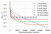
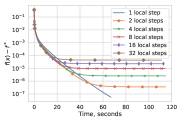
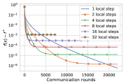
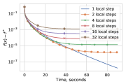
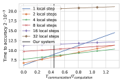
Since our architecture leads to a very specific trade-off between computation and communication, we also provide plots for the case the communication time relative to gradient computation time is higher or lower. In all experiments, we use full gradients and constant stepsize . The amount of regularization was chosen of order , where is the total amount of data. The data partitioning is not i.i.d. and is done based on the index in the original dataset.
We observe a very tight match between our theory and numerical results. In cases where communication is significantly more expensive than gradient computation, local methods are much faster for imprecise convergence. This was not a big advantage though with our architecture, mainly because full gradients took a lot of time to be computed.

References
- Basu et al. [2019] Debraj Basu, Deepesh Data, Can Karakus, and Suhas Diggavi. Qsparse-local-SGD: Distributed SGD with Quantization, Sparsification, and Local Computations. arXiv:1906.02367, 2019.
- Chang and Lin [2011] Chih-Chung Chang and Chih-Jen Lin. LIBSVM: A library for support vector machines. ACM Transactions on Intelligent Systems and Technology (TIST), 2(3):27, 2011.
- Chavdarova et al. [2019] Tatjana Chavdarova, Gauthier Gidel, François Fleuret, and Simon Lacoste-Julien. Reducing Noise in GAN Training with Variance Reduced Extragradient. arXiv preprint arXiv:1904.08598, 2019.
- Dalcin et al. [2011] Lisandro D. Dalcin, Rodrigo R. Paz, Pablo A. Kler, and Alejandro Cosimo. Parallel distributed computing using Python. Advances in Water Resources, 34(9):1124–1139, 2011.
- Hard et al. [2018] Andrew Hard, Kanishka Rao, Rajiv Mathews, Françoise Beaufays, Sean Augenstein, Hubert Eichner, Chloé Kiddon, and Daniel Ramage. Federated Learning for Mobile Keyboard Prediction. arXiv:1811.03604, 2018.
- Juditsky et al. [2011] Anatoli Juditsky, Arkadi Nemirovski, and Claire Tauvel. Solving variational Inequalities with Stochastic Mirror-Prox algorithm. Stochastic Systems, 1(1):17–58, 2011.
- Konečný et al. [2016] Jakub Konečný, H. Brendan McMahan, Felix X. Yu, Peter Richtárik, Ananda Theertha Suresh, and Dave Bacon. Federated Learning: Strategies for Improving Communication Efficiency. In NIPS Private Multi-Party Machine Learning Workshop, 2016.
- Li et al. [2019] Xiang Li, Kaixuan Huang, Wenhao Yang, Shusen Wang, and Zhihua Zhang. On the Convergence of FedAvg on Non-IID Data. arXiv:1907.02189, 2019.
- Mangasarian [1995] L. Mangasarian. Parallel Gradient Distribution in Unconstrained Optimization. SIAM Journal on Control and Optimization, 33(6):1916–1925, 1995.
- McMahan et al. [2016] H. Brendan McMahan, Eider Moore, Daniel Ramage, Seth Hampson, and Blaise Agüera y Arcas. Communication-Efficient Learning of Deep Networks from Decentralized Data. Proceedings of the 20 th International Conference on Artificial Intelligence and Statistics (AISTATS) 2017. JMLR: W&CP volume 54, 2016.
- Mishchenko et al. [2018] Konstantin Mishchenko, Franck Iutzeler, Jérôme Malick, and Massih-Reza Amini. A Delay-tolerant Proximal-Gradient Algorithm for Distributed Learning. In International Conference on Machine Learning, pages 3584–3592, 2018.
- Mishchenko et al. [2019] Konstantin Mishchenko, Dmitry Kovalev, Egor Shulgin, Peter Richtárik, and Yura Malitsky. Revisiting Stochastic Extragradient. arXiv preprint arXiv:1905.11373, 2019.
- Sahu et al. [2018] Anit Kumar Sahu, Tian Li, Maziar Sanjabi, Manzil Zaheer, Ameet Talwalkar, and Virginia Smith. On the Convergence of Federated Optimization in Heterogeneous Networks. arXiv:1812.06127, 2018.
- Stich [2018] Sebastian U. Stich. Local SGD Converges Fast and Communicates Little. arXiv:1805.09767, 2018.
- Wang and Joshi [2018] Jianyu Wang and Gauri Joshi. Cooperative SGD: A Unified Framework for the Design and Analysis of Communication-Efficient SGD Algorithms. arXiv:1808.07576, 2018.
- Wang et al. [2018] Shiqiang Wang, Tiffany Tuor, Theodoros Salonidis, Kin K. Leung, Christian Makaya, Ting He, and Kevin Chan. When Edge Meets Learning: Adaptive Control for Resource-Constrained Distributed Machine Learning. arXiv:1804.05271, 2018.
- Yu et al. [2018] Hao Yu, Sen Yang, and Shenghuo Zhu. Parallel Restarted SGD with Faster Convergence and Less Communication: Demystifying Why Model Averaging Works for Deep Learning. arXiv:1807.06629, 2018.
- Yu et al. [2019] Hao Yu, Rong Jin, and Sen Yang. On the Linear Speedup Analysis of Communication Efficient Momentum SGD for Distributed Non-Convex Optimization. arXiv preprint arXiv:1905.03817, 2019.
- Zhou and Cong [2018] Fan Zhou and Guojing Cong. On the Convergence Properties of a -step Averaging Stochastic Gradient Descent Algorithm for Nonconvex Optimization. In IJCAI International Joint Conference on Artificial Intelligence, volume 2018-July, pages 3219–3227, 2018.
Supplementary Material for:
First Analysis of Local GD on Heterogeneous Data
4 Proofs
We first provide two technical lemmas which relate the quantities , and , and for . These lemmas are independent of the algorithm.
Lemma 3.
If Assumption 1 holds, then
| (7) |
Proof.
Starting with the left-hand side,
where in the second inequality we have used convexity of the map . The claim of the lemma follows by noting that
∎
Lemma 4.
Suppose that Assumption 1 holds. Then,
| (8) |
Proof.
Starting with the left-hand side,
| (9) |
The first term in (9) is bounded by convexity:
| (10) |
For the second term, we use -smoothness,
| (11) |
Combining (11) and (10) in (9),
Averaging over ,
Note that the first term is the Bregman divergence and the second term is just , hence
which is the claim of this lemma. ∎
Proof of Lemma 1.
Proof of Lemma 2.
Let , then noting that when and we have,
Then we have
Putting , , we get
Averaging with respect to ,
Hence we have,
Summing up the above inequality as varies from to ,
Noting that the sum appears on both sides, we have
Note that because , then our choice of implies that , hence
For the second part, we have
Using that we get that , and using this we get the second claim. ∎
Proof of Theorem 1.
Starting with Lemma 1, we have
Summing up these inequalities gives
and using that for some , we can decompose the second term by double counting and bound it by Lemma 2, then using double counting again,
Using this in the previous bound,
Rearranging we get,
Dividing both sides by we get,
Finally, using Jensen’s inequality and the convexity of we get the required claim. ∎