A multiresolution algorithm to approximate the Hutchinson measure for IFS and GIFS

Rudnei D. da Cunha Instituto de Matemática e Estatística - UFRGS, Av. Bento Gonçalves 9500, 91500-900 Porto Alegre - RS - Brazil.
E-mail: rudnei.cunha@ufrgs.br Universidade Federal do Rio Grande do Sul
Elismar R. Oliveira E-mail: elismar.oliveira@ufrgs.br Universidade Federal do Rio Grande do Sul Filip Strobin Instititute of Mathematics, Lodz University of Technology, Wólczańska 215, 90-924 Łódź, Poland. Lodz University of Technology
(March 2, 2024)
Abstract

We introduce a discrete version of the Hutchinson–Barnsley theory providing algorithms to approximate the Hutchinson measure for iterated function systems (IFS) and generalized iterated function systems (GIFS), complementing the discrete version of the deterministic algorithm considered in our previous work.


Key words and phrases: iterated function system (IFS), generalized iterated function system (GIFS), Markov operator, invariant measures, Hutchinson measures, attractor, discrete deterministic algorithm, discretization.

2010 Mathematics Subject Classification: Primary 28A80; Secondary 37C70, 41A65, 65S05, 65P99.

1 Introduction

This work is a sequel of [dOS20] where we approximate attractors for IFS and GIFS and their fuzzy versions by a discrete version of the deterministic algorithm.

Here we adapt the introduced theory to find a discrete version of the Markov operator acting on probability measures. Once we prove that this operator satisfies the assumptions of the discrete version of the Banach fixed point theorem (Theorem 3.2), we justify the existence of a discrete measure approximating the Hutchinson Measure associated to the underlying IFS or GIFS with probabilities. This fits to problems addressed by several authors such as [Öbe05], [Öbe06], [Bla01], [Fro99], [GN14], [GMN16] and [CJ19]. See the introduction of [GMN16] for a detailed review on the advances of most of these references.

In recent years some authors have made significant advances in the task of giving an approximation of the invariant measure of a dynamical system with precisely estimated error. For example, the strategy in [GMN16] is to replace the original Markov (transfer) operator, let us say M𝑀M, by a finite rank one, let us say M~~𝑀\tilde{M}. Then the authors use some powerful techniques and a functional analytic approach to approximate the actual invariant measure μ𝜇\mu (i.e. M(μ)=μ𝑀𝜇𝜇M(\mu)=\mu) by the fixed point μ~~𝜇\tilde{\mu} of M~~𝑀\tilde{M}. Our approach is different: modifying the original IFS 𝒮𝒮\mathcal{S} by replacing its maps with their certain discretizations defined on appropriately dense grids, we obtain a new IFS S^^𝑆\hat{S}, whose Markov operator M^^𝑀\hat{M} need not be contractive (see Example 5.3), but its iterations give approximations of the invariant measure of 𝒮𝒮\mathcal{S}. Not only we present an algorithm that approximates the invariant measure for an IFS with probabilities but, similarly as in [GMN16], we provide an explicit control on the convergence and the error estimation. The main novelty is the fact that we can apply this procedure even for generalized iterated function systems which have no dynamical counterpart, presenting, as far as we know, the first rigorous computation of the invariant measures in the literature, including place depending probabilities. The advantages of our approach (discretization of the space and of the associated operators) is that we obtain a very simple algorithm to be coded exhibiting an outstanding performance for computation without the need of a sophisticated computational machinery. Moreover, the lack of requirements allow us to extrapolate the application of the algorithm to investigate (heuristically) other situations where our hypothesis fail, for instance as in Example 6.5 where the convergence can not happen since we have more than one invariant measures.

In Example 5.7 we make a comparative analysis between our algorithm and the method employed in [GMN16] for a contracting case. Also, in Section 6, subsection 6.1, we make a comparison between our computations and with the computational results given in a recent preprint [CJ19]. It is worth to mention that [CJ19] follows a very different approach to the problem: the maps are also assumed to be Lipschitz contractions but the authors use an operator theoretic approach similar to that given in [JP07] where the family of maps must be complex contracting leading to a good numerical results.

The paper is organized as follows:
In Section 2 we recall some basic facts on the Hutchinson–Barnsley theory and its certain generalization due to Miculescu and Mihail. Not only we formulate the Hutchinson-Barnsley theorem on the existence of attractors, but also, we recall definition of (generalized) Markov operator and provide theorems on the existence the Hutchinson measure.

After, in Section 3, we present the theory developed in [dOS20]. We formulate a discrete version of the Banach fixed point theory and present its application - discretizations of the Hutchinson-Barnsley theorem, as well as its generalization due to Miculescu and Mihail.

In Section 4 we obtain the main result of our paper, which shows that we can approximate the Hutchinson measure of given IFS (or GIFS) by appropriate discrete measure, obtained by iterating process of discrete Markov operator.

In Section 5 we introduce an algorithm that can be used to generate discrete Hutchinson measures (for IFSs and GIFSs) and also we present some examples to illustrate it. Note that our algorithm draw the pictures of approximations of the attractors both of IFSs and GIFSs. Other such algorithms for GIFSs can be found in [JMS16] and [MMU20].

Finally in Section 6 we address the problem of estimating the integral of functions with respect to the Hutchinson measures from [CJ19], the problem of the Projected Hutchinson measures from [Oli17] and the problem of IFS/GIFS with place dependent probabilities from [Mic14].

Note that some results we recall in the initial sections (for example, Lemmas 2.3 and 2.11, and Sections 3.2 and 3.3) are given just for the sake of completeness and for the reader’s convenience.

2 Basics of the Hutchinson–Barnsley theory and its certain generalization

2.1 Iterated function systems and the Hutchinson–Barnsley theorem

Let (X,d)𝑋𝑑(X,d) be a metric space. We say that f:XX:𝑓𝑋𝑋f:X\to X is a Banach contraction, if the Lipschitz constant Lip(f)<1Lip𝑓1\operatorname{Lip}(f)<1.

Definition 2.1.

An iterated function system (IFS in short) 𝒮=(X,(ϕj)j=1L)𝒮𝑋superscriptsubscriptsubscriptitalic-ϕ𝑗𝑗1𝐿\mathcal{S}=(X,(\phi_{j})_{j=1}^{L}) consists of a finite family ϕ1,,ϕLsubscriptitalic-ϕ1subscriptitalic-ϕ𝐿\phi_{1},...,\phi_{L} of continuous selfmaps of X𝑋X. Each IFS 𝒮𝒮\mathcal{S} generates the map F𝒮:𝒦(X)𝒦(X):subscript𝐹𝒮𝒦𝑋𝒦𝑋F_{\mathcal{S}}:\mathcal{K}(X)\to\mathcal{K}(X) (where 𝒦(X)𝒦𝑋\mathcal{K}(X) denotes the family of all nonempty and compact subsets of X𝑋X), called the Hutchinson operator, defined by

K𝒦(X)F𝒮(K):=j=1Lϕj(K).assignsubscriptfor-all𝐾𝒦𝑋subscript𝐹𝒮𝐾superscriptsubscript𝑗1𝐿subscriptitalic-ϕ𝑗𝐾\forall_{K\in\mathcal{K}(X)}\;F_{\mathcal{S}}(K):=\bigcup_{j=1}^{L}\phi_{j}(K).

By an attractor of an IFS 𝒮𝒮\mathcal{S} we mean a (necessarily unique) set A𝒮𝒦(X)subscript𝐴𝒮𝒦𝑋A_{\mathcal{S}}\in\mathcal{K}(X) which satisfies

A𝒮=F𝒮(A𝒮)=j=1Lϕj(A𝒮)subscript𝐴𝒮subscript𝐹𝒮subscript𝐴𝒮superscriptsubscript𝑗1𝐿subscriptitalic-ϕ𝑗subscript𝐴𝒮A_{\mathcal{S}}=F_{\mathcal{S}}(A_{\mathcal{S}})=\bigcup_{j=1}^{L}\phi_{j}(A_{\mathcal{S}})

and such that for every K𝒦(X)𝐾𝒦𝑋K\in\mathcal{K}(X), the sequence of iterates (F𝒮k(K))k=0superscriptsubscriptsuperscriptsubscript𝐹𝒮𝑘𝐾𝑘0(F_{\mathcal{S}}^{k}(K))_{k=0}^{\infty} converges to A𝒮subscript𝐴𝒮A_{\mathcal{S}} with respect to the Hausdorff-Pompeiu metric hh on 𝒦(X)𝒦𝑋\mathcal{K}(X)(see [BP13] for details on the Hausdorff-Pompeiu metric).

The classical Hutchinson–Barnsley theorem [Bar88], [Hut81] states that:

Theorem 2.2.

Each IFS 𝒮𝒮\mathcal{S} consisting of Banach contractions on a complete metric space X𝑋X admits attractor.

This result can be proved with a help of the Banach fixed point theorem as it turns out that F𝒮subscript𝐹𝒮F_{\mathcal{S}} is a Banach contraction provided each ϕjsubscriptitalic-ϕ𝑗\phi_{j} is a Banach contraction (see, for example, [Hut81, Section 3.2]):

Lemma 2.3.

Let (X,d)𝑋𝑑(X,d) be a metric space and 𝒮=(X,(ϕj)j=1L)𝒮𝑋superscriptsubscriptsubscriptitalic-ϕ𝑗𝑗1𝐿\mathcal{S}=(X,(\phi_{j})_{j=1}^{L}) be an IFS consisting of Banach contractions. Then F𝒮subscript𝐹𝒮F_{\mathcal{S}} is a Banach contraction and Lip(F𝒮)max{Lip(ϕj):j=1,,L}Lipsubscript𝐹𝒮:Lipsubscriptitalic-ϕ𝑗𝑗1𝐿\operatorname{Lip}(F_{\mathcal{S}})\leq\max\{\operatorname{Lip}(\phi_{j}):j=1,...,L\}.

Given an IFS 𝒮=(X,(ϕj)j=1L)𝒮𝑋superscriptsubscriptsubscriptitalic-ϕ𝑗𝑗1𝐿\mathcal{S}=(X,(\phi_{j})_{j=1}^{L}) consisting of Banach contractions, we will denote

α𝒮:=max{Lip(ϕ1),,Lip(ϕL)}.assignsubscript𝛼𝒮Lipsubscriptitalic-ϕ1Lipsubscriptitalic-ϕ𝐿\alpha_{\mathcal{S}}:=\max\{\operatorname{Lip}(\phi_{1}),...,\operatorname{Lip}(\phi_{L})\}.

2.2 IFSs with probabilities and the Hutchinson measure

For a metric space (X,d)𝑋𝑑(X,d), by 𝒫(X)𝒫𝑋\mathcal{P}(X) we denote the family of all nonnegative Borel probability measures μ𝜇\mu with compact support, that is, for which there exists a compact set K𝐾K so that μ(XK)=0𝜇𝑋𝐾0\mu(X\setminus K)=0. For every μ,ν𝒫(X)𝜇𝜈𝒫𝑋\mu,\nu\in\mathcal{P}(X), define

dMK(μ,ν)=sup{|XfdμXfdν|:fLip1(X,)},d_{MK}(\mu,\nu)=\sup\left\{\left|\int_{X}f\mathrm{d}\mu-\int_{X}f\mathrm{d}\nu\right|:f\in\operatorname{Lip}_{1}(X,\mathbb{R})\right\}, (1)

where Lip1(X,)subscriptLip1𝑋\operatorname{Lip}_{1}(X,\mathbb{R}) is the set of maps f:X:𝑓𝑋f:X\to\mathbb{R} with Lip(f)1Lip𝑓1\operatorname{Lip}(f)\leq 1. It is known (see [Bog07],[KLMV12],[Hut81], [Bar88]) that dMKsubscript𝑑𝑀𝐾d_{MK} is a metric, and it is complete provided (X,d)𝑋𝑑(X,d) is complete. The metric dMKsubscript𝑑𝑀𝐾d_{MK} is called the Monge-Kantorovich metric or the Hutchinson metric.
For a Borel measurable map w:XY:𝑤𝑋𝑌w:X\to Y (where Y𝑌Y is a metric space) and μ𝒫(X)𝜇𝒫𝑋\mu\in\mathcal{P}(X), by wμsuperscript𝑤𝜇w^{\sharp}\mu we denote the measure on Y𝑌Y defined by

wμ(B):=μ(w1(B)).assignsuperscript𝑤𝜇𝐵𝜇superscript𝑤1𝐵w^{\sharp}\mu(B):=\mu(w^{-1}(B)). (2)

It is known that wμ𝒫(Y)superscript𝑤𝜇𝒫𝑌w^{\sharp}\mu\in\mathcal{P}(Y) and that for any continuous map f:Y:𝑓𝑌f:Y\to\mathbb{R} and every μ𝒫(X)𝜇𝒫𝑋\mu\in\mathcal{P}(X),

Xf𝑑wμ=Xfw𝑑μ.subscript𝑋𝑓differential-dsuperscript𝑤𝜇subscript𝑋𝑓𝑤differential-d𝜇\int_{X}f\;dw^{\sharp}\mu=\int_{X}f\circ w\;d\mu. (3)
Definition 2.4.

By an IFS with probabilities (IFSp in short) we mean a triple 𝒮=(X,(ϕj)j=1L,(pj)j=1L)𝒮𝑋superscriptsubscriptsubscriptitalic-ϕ𝑗𝑗1𝐿superscriptsubscriptsubscript𝑝𝑗𝑗1𝐿\mathcal{S}=(X,(\phi_{j})_{j=1}^{L},(p_{j})_{j=1}^{L}) so that (X,(ϕj)j=1L)𝑋superscriptsubscriptsubscriptitalic-ϕ𝑗𝑗1𝐿(X,(\phi_{j})_{j=1}^{L}) is an IFS and p1,,pL>0subscript𝑝1subscript𝑝𝐿0p_{1},...,p_{L}>0 with j=1Lpj=1superscriptsubscript𝑗1𝐿subscript𝑝𝑗1\sum_{j=1}^{L}p_{j}=1.
Each IFSp generates the map M𝒮:𝒫(X)𝒫(X):subscript𝑀𝒮𝒫𝑋𝒫𝑋M_{\mathcal{S}}:\mathcal{P}(X)\to\mathcal{P}(X), called the
Markov operator, which adjust to every μ𝒫(X)𝜇𝒫𝑋\mu\in\mathcal{P}(X), the measure M𝒮(μ)subscript𝑀𝒮𝜇M_{\mathcal{S}}(\mu) defined by:

M𝒮(μ)(B)=j=1Lpjμ(ϕj1(B))=j=1Lpjϕjμ,subscript𝑀𝒮𝜇𝐵superscriptsubscript𝑗1𝐿subscript𝑝𝑗𝜇superscriptsubscriptitalic-ϕ𝑗1𝐵superscriptsubscript𝑗1𝐿subscript𝑝𝑗superscriptsubscriptitalic-ϕ𝑗𝜇M_{\mathcal{S}}(\mu)(B)=\sum_{j=1}^{L}p_{j}\mu\left(\phi_{j}^{-1}(B)\right)=\sum_{j=1}^{L}p_{j}\phi_{j}^{\sharp}\mu,\quad

for any Borel set BX𝐵𝑋B\subset X.
By a Hutchinson measure of an IFSp 𝒮𝒮\mathcal{S} we mean a (necessarily unique) measure μ𝒮𝒫(X)subscript𝜇𝒮𝒫𝑋\mu_{\mathcal{S}}\in\mathcal{P}(X) which satisfies

μ𝒮=M𝒮(μ𝒮)subscript𝜇𝒮subscript𝑀𝒮subscript𝜇𝒮\mu_{\mathcal{S}}=M_{\mathcal{S}}(\mu_{\mathcal{S}}) (4)

and such that for every μ𝒫(X)𝜇𝒫𝑋\mu\in\mathcal{P}(X), the sequence of iterates M𝒮k(μ)subscriptsuperscript𝑀𝑘𝒮𝜇M^{k}_{\mathcal{S}}(\mu) converges to μ𝒮subscript𝜇𝒮\mu_{\mathcal{S}} with respect to dMKsubscript𝑑𝑀𝐾d_{MK}.

Observe that by (3), for every IFSp 𝒮𝒮\mathcal{S} and every continuous map f:X:𝑓𝑋f:X\to\mathbb{R},

Xf𝑑M𝒮(μ)=j=1LpjXfϕj𝑑μ.subscript𝑋𝑓differential-dsubscript𝑀𝒮𝜇superscriptsubscript𝑗1𝐿subscript𝑝𝑗subscript𝑋𝑓subscriptitalic-ϕ𝑗differential-d𝜇\int_{X}f\;dM_{\mathcal{S}}(\mu)=\sum_{j=1}^{L}p_{j}\int_{X}f\circ\phi_{j}\;d\mu. (5)

In fact, the above formula characterizes the Markov operator M𝒮subscript𝑀𝒮M_{\mathcal{S}}. The following result is known (see mentioned papers, for example [Hut81, Section 4.4]).

Theorem 2.5.

Each IFSp on a complete metric space consisting of Banach contractions admits the Hutchinson measure.

This result can be proved with a help of the Banach fixed point theorem as the following lemma holds:

Lemma 2.6.

If an IFSp 𝒮𝒮\mathcal{S} consists of Banach contractions, then M𝒮subscript𝑀𝒮M_{\mathcal{S}} is a Banach contraction and Lip(M𝒮)α𝒮Lipsubscript𝑀𝒮subscript𝛼𝒮\operatorname{Lip}(M_{\mathcal{S}})\leq\alpha_{\mathcal{S}}.

For a measure μ𝒫(X)𝜇𝒫𝑋\mu\in\mathcal{P}(X), by its support we mean the set

supp(μ)={xX:μ(U)>0for all open setsUx}.supp𝜇conditional-set𝑥𝑋𝜇𝑈0for all open sets𝑈contains𝑥\operatorname{supp}(\mu)=\{x\in X:\mu(U)>0\;\mbox{for all open sets}\;U\ni x\}.

Alternatively, supp(μ)supp𝜇\operatorname{supp}(\mu) is the largest compact set C𝐶C such that μ(U)>0𝜇𝑈0\mu(U)>0 for every open set U𝑈U with UC𝑈𝐶U\cap C\neq\emptyset. The following result shows that there is a strong relationship between the Markov and Hutchinson operators. It implies that the support of the Hutchinson measure is exactly the attractor for a given IFS (see [Hut81, Section 4.4, Thm. 4]).

Lemma 2.7.

In the above frame, for every μ𝒫(X)𝜇𝒫𝑋\mu\in\mathcal{P}(X), supp(M𝒮(μ))=F𝒮(supp(μ))suppsubscript𝑀𝒮𝜇subscript𝐹𝒮supp𝜇\operatorname{supp}(M_{\mathcal{S}}(\mu))=F_{\mathcal{S}}(\operatorname{supp}(\mu)).

2.3 Generalized IFSs in the sense of Miculescu and Mihail

Here we recall some basics of a generalization of the classical IFS theory introduced by R. Miculescu and A. Mihail in 2008. For references, see [Mih08], [MM10], [MM08], [SS13] and references therein.
If (X,d)𝑋𝑑(X,d) is a metric space and m𝑚m\in\mathbb{N}, then by Xmsuperscript𝑋𝑚X^{m} we denote the Cartesian product of m𝑚m copies of X𝑋X. We consider it as a metric space with the maximum metric

dm((x0,,xm1),(y0,,ym1)):=max{d(x0,y0),,d(xm1,ym1)}.assignsubscript𝑑𝑚subscript𝑥0subscript𝑥𝑚1subscript𝑦0subscript𝑦𝑚1𝑑subscript𝑥0subscript𝑦0𝑑subscript𝑥𝑚1subscript𝑦𝑚1d_{m}((x_{0},...,x_{m-1}),(y_{0},...,y_{m-1})):=\max\{d(x_{0},y_{0}),...,d(x_{m-1},y_{m-1})\}.

A map f:XmX:𝑓superscript𝑋𝑚𝑋f:X^{m}\to X is called a generalized Banach contraction, if Lip(f)<1Lip𝑓1\operatorname{Lip}(f)<1.

It turns out that a counterpart of the Banach fixed point theorem holds. Namely, if f:XmX:𝑓superscript𝑋𝑚𝑋f:X^{m}\to X is a generalized Banach contraction, then there is a unique point xXsubscript𝑥𝑋x_{*}\in X (called a generalized fixed point of f𝑓f), such that f(x,,x)=x𝑓subscript𝑥subscript𝑥subscript𝑥f(x_{*},...,x_{*})=x_{*}. Moreover, for every x0,,xm1Xsubscript𝑥0subscript𝑥𝑚1𝑋x_{0},...,x_{m-1}\in X, the sequence (xk)subscript𝑥𝑘(x_{k}) defined by

xk+m=f(xk,,xk+m1),k0,formulae-sequencesubscript𝑥𝑘𝑚𝑓subscript𝑥𝑘subscript𝑥𝑘𝑚1𝑘0x_{k+m}=f(x_{k},...,x_{k+m-1}),\;\;k\geq 0,

converges to xsubscript𝑥x_{*}.

Remark 2.8.

It is worth to observe that if f:XmX:𝑓superscript𝑋𝑚𝑋f:X^{m}\to X is a generalized Banach contraction, then the map f~:XX:~𝑓𝑋𝑋\tilde{f}:X\to X defined by f~(x):=f(x,,x)assign~𝑓𝑥𝑓𝑥𝑥\tilde{f}(x):=f(x,...,x), is a Banach contraction and Lip(f~)Lip(f)Lip~𝑓Lip𝑓\operatorname{Lip}(\tilde{f})\leq\operatorname{Lip}(f).

Definition 2.9.

A generalized iterated function system of order m𝑚m (GIFS in short) 𝒮=(X,(ϕj)j=1L)𝒮𝑋superscriptsubscriptsubscriptitalic-ϕ𝑗𝑗1𝐿\mathcal{S}=(X,(\phi_{j})_{j=1}^{L}) consists of a finite family ϕ1,,ϕLsubscriptitalic-ϕ1subscriptitalic-ϕ𝐿\phi_{1},...,\phi_{L} of continuous maps from Xmsuperscript𝑋𝑚X^{m} to X𝑋X. Each GIFS 𝒮𝒮\mathcal{S} generates the map F𝒮:𝒦(X)m𝒦(X):subscript𝐹𝒮𝒦superscript𝑋𝑚𝒦𝑋F_{\mathcal{S}}:\mathcal{K}(X)^{m}\to\mathcal{K}(X), called the generalized Hutchinson operator , defined by

K0,,Km1𝒦(X)F𝒮(K0,,Km1):=j=1Lϕj(K0××Km1).assignsubscriptfor-allsubscript𝐾0subscript𝐾𝑚1𝒦𝑋subscript𝐹𝒮subscript𝐾0subscript𝐾𝑚1superscriptsubscript𝑗1𝐿subscriptitalic-ϕ𝑗subscript𝐾0subscript𝐾𝑚1\forall_{K_{0},...,K_{m-1}\in\mathcal{K}(X)}\;F_{\mathcal{S}}(K_{0},...,K_{m-1}):=\bigcup_{j=1}^{L}\phi_{j}(K_{0}\times...\times K_{m-1}).

By an attractor of a GIFS 𝒮𝒮\mathcal{S} we mean a (necessarily unique) set A𝒮𝒦(X)subscript𝐴𝒮𝒦𝑋A_{\mathcal{S}}\in\mathcal{K}(X) which satisfies

A𝒮=F𝒮(A𝒮,,A𝒮)=j=1Lϕj(A𝒮××A𝒮)subscript𝐴𝒮subscript𝐹𝒮subscript𝐴𝒮subscript𝐴𝒮superscriptsubscript𝑗1𝐿subscriptitalic-ϕ𝑗subscript𝐴𝒮subscript𝐴𝒮A_{\mathcal{S}}=F_{\mathcal{S}}(A_{\mathcal{S}},...,A_{\mathcal{S}})=\bigcup_{j=1}^{L}\phi_{j}(A_{\mathcal{S}}\times...\times A_{\mathcal{S}})

and such that for every K0,,Km𝒦(X)subscript𝐾0subscript𝐾𝑚𝒦𝑋K_{0},...,K_{m}\in\mathcal{K}(X), the sequence (Kk)subscript𝐾𝑘(K_{k}) defined by

Kk+m:=F𝒮(Kk,,Kk+m1),k0,formulae-sequenceassignsubscript𝐾𝑘𝑚subscript𝐹𝒮subscript𝐾𝑘subscript𝐾𝑘𝑚1𝑘0K_{k+m}:=F_{\mathcal{S}}(K_{k},...,K_{k+m-1}),\;\;k\geq 0,

converges to A𝒮subscript𝐴𝒮A_{\mathcal{S}}.

Theorem 2.10.

Each GIFS 𝒮𝒮\mathcal{S} on a complete metric space consisting of generalized Banach contractions generates the (unique) attractor A𝒮subscript𝐴𝒮A_{\mathcal{S}}.

This result can be proved with a help of a certain generalization of the Banach fixed point theorem as it turns out that F𝒮subscript𝐹𝒮F_{\mathcal{S}} is a Banach contraction provided each ϕjsubscriptitalic-ϕ𝑗\phi_{j} is a Banach contraction (see, for example, [MM10, Lemma 3.6]):

Lemma 2.11.

Let (X,d)𝑋𝑑(X,d) be a metric space and 𝒮=(X,(ϕj)j=1L)𝒮𝑋superscriptsubscriptsubscriptitalic-ϕ𝑗𝑗1𝐿\mathcal{S}=(X,(\phi_{j})_{j=1}^{L}) be a GIFS consisting of generalized Banach contractions. Then F𝒮subscript𝐹𝒮F_{\mathcal{S}} is a generalized Banach contraction with Lip(F𝒮)α𝒮:=max{Lip(ϕj):j=1,,L}Lipsubscript𝐹𝒮subscript𝛼𝒮assign:Lipsubscriptitalic-ϕ𝑗𝑗1𝐿\operatorname{Lip}(F_{\mathcal{S}})\leq\alpha_{\mathcal{S}}:=\max\{\operatorname{Lip}(\phi_{j}):j=1,...,L\}.

In [Mih09] and [MM09], Miculescu and Mihail studied the counterpart of the Hutchinson measure for GIFSs.

Definition 2.12.

By a GIFS with probabilities (GIFSp in short) we mean a triple 𝒮=(X,(ϕj)j=1L,(pj)j=1L)𝒮𝑋superscriptsubscriptsubscriptitalic-ϕ𝑗𝑗1𝐿superscriptsubscriptsubscript𝑝𝑗𝑗1𝐿\mathcal{S}=(X,(\phi_{j})_{j=1}^{L},(p_{j})_{j=1}^{L}) so that (X,(ϕj)j=1L)𝑋superscriptsubscriptsubscriptitalic-ϕ𝑗𝑗1𝐿(X,(\phi_{j})_{j=1}^{L}) is a GIFS and p1,,pL>0subscript𝑝1subscript𝑝𝐿0p_{1},...,p_{L}>0 with j=1Lpj=1superscriptsubscript𝑗1𝐿subscript𝑝𝑗1\sum_{j=1}^{L}p_{j}=1.
Each GIFSp generates the map M𝒮:𝒫(X)m𝒫(X):subscript𝑀𝒮𝒫superscript𝑋𝑚𝒫𝑋M_{\mathcal{S}}:\mathcal{P}(X)^{m}\to\mathcal{P}(X), called the
generalized Markov operator which adjust to any μ0,,μm1𝒫(X)subscript𝜇0subscript𝜇𝑚1𝒫𝑋\mu_{0},...,\mu_{m-1}\in\mathcal{P}(X), the measure M𝒮(μ0,,μm1)subscript𝑀𝒮subscript𝜇0subscript𝜇𝑚1M_{\mathcal{S}}(\mu_{0},...,\mu_{m-1}) defined by

M𝒮(μ0,,μm1)(B):=j=1Lpj(μ××μm1)(ϕj1(B))=j=1Lpjϕj(μ0××μm1)(B),assignsubscript𝑀𝒮subscript𝜇0subscript𝜇𝑚1𝐵superscriptsubscript𝑗1𝐿subscript𝑝𝑗𝜇subscript𝜇𝑚1superscriptsubscriptitalic-ϕ𝑗1𝐵superscriptsubscript𝑗1𝐿subscript𝑝𝑗superscriptsubscriptitalic-ϕ𝑗subscript𝜇0subscript𝜇𝑚1𝐵M_{\mathcal{S}}(\mu_{0},...,\mu_{m-1})(B):=\sum_{j=1}^{L}p_{j}(\mu\times...\times\mu_{m-1})(\phi_{j}^{-1}(B))=\sum_{j=1}^{L}p_{j}\phi_{j}^{\sharp}(\mu_{0}\times...\times\mu_{m-1})(B),\quad

for any Borel set BX𝐵𝑋B\subset X, and where μ0××μm1subscript𝜇0subscript𝜇𝑚1\mu_{0}\times...\times\mu_{m-1} is the product measure.
By the
generalized Hutchinson measure of a GIFSp 𝒮𝒮\mathcal{S} we mean the unique measure μ𝒮𝒫(X)subscript𝜇𝒮𝒫𝑋\mu_{\mathcal{S}}\in\mathcal{P}(X) which satisfies

μ𝒮=M𝒮(μ𝒮,,μ𝒮)subscript𝜇𝒮subscript𝑀𝒮subscript𝜇𝒮subscript𝜇𝒮\mu_{\mathcal{S}}=M_{\mathcal{S}}(\mu_{\mathcal{S}},...,\mu_{\mathcal{S}}) (6)

and such that for every μ0,,μm1𝒫(X)subscript𝜇0subscript𝜇𝑚1𝒫𝑋\mu_{0},...,\mu_{m-1}\in\mathcal{P}(X), the sequence (μk)subscript𝜇𝑘(\mu_{k}) defined by μm+k:=M𝒮(μk,,μk+m1)assignsubscript𝜇𝑚𝑘subscript𝑀𝒮subscript𝜇𝑘subscript𝜇𝑘𝑚1\mu_{m+k}:=M_{\mathcal{S}}(\mu_{k},...,\mu_{k+m-1}), converges to μ𝒮subscript𝜇𝒮\mu_{\mathcal{S}} with respect to dMKsubscript𝑑𝑀𝐾d_{MK}.

Once again we observe that by (3), for every IFSp 𝒮𝒮\mathcal{S} and every continuous map f:X:𝑓𝑋f:X\to\mathbb{R},

Xf𝑑M𝒮(μ0,,μm1)=j=1LpjXmfϕjd(μ0××μm1).subscript𝑋𝑓differential-dsubscript𝑀𝒮subscript𝜇0subscript𝜇𝑚1superscriptsubscript𝑗1𝐿subscript𝑝𝑗subscriptsuperscript𝑋𝑚𝑓subscriptitalic-ϕ𝑗𝑑subscript𝜇0subscript𝜇𝑚1\int_{X}f\;dM_{\mathcal{S}}(\mu_{0},...,\mu_{m-1})=\sum_{j=1}^{L}p_{j}\int_{X^{m}}f\circ\phi_{j}\;d(\mu_{0}\times...\times\mu_{m-1}). (7)

For m𝑚m\in\mathbb{N} and a0,,am10subscript𝑎0subscript𝑎𝑚10a_{0},...,a_{m-1}\geq 0, we say that f:XmX:𝑓superscript𝑋𝑚𝑋f:X^{m}\to X is a (a0,,am1)subscript𝑎0subscript𝑎𝑚1(a_{0},...,a_{m-1})-contraction, if

(x0,,xm1),(y0,,ym1)Xmd(f(x0,,xm1),f(y0,,ym1))j=0m1ajd(xj,yj)subscriptfor-allsubscript𝑥0subscript𝑥𝑚1subscript𝑦0subscript𝑦𝑚1superscript𝑋𝑚𝑑𝑓subscript𝑥0subscript𝑥𝑚1𝑓subscript𝑦0subscript𝑦𝑚1superscriptsubscript𝑗0𝑚1subscript𝑎𝑗𝑑subscript𝑥𝑗subscript𝑦𝑗\forall_{(x_{0},...,x_{m-1}),(y_{0},...,y_{m-1})\in X^{m}}\;d(f(x_{0},...,x_{m-1}),f(y_{0},...,y_{m-1}))\leq\sum_{j=0}^{m-1}a_{j}d(x_{j},y_{j}) (8)

It is easy to see that the Lipschitz constant of (a0,,am1)subscript𝑎0subscript𝑎𝑚1(a_{0},...,a_{m-1})-contraction f𝑓f is bounded by Lip(f)j=0m1ajLip𝑓superscriptsubscript𝑗0𝑚1subscript𝑎𝑗\operatorname{Lip}(f)\leq\sum_{j=0}^{m-1}a_{j}. In particular, if j=0m1aj<1superscriptsubscript𝑗0𝑚1subscript𝑎𝑗1\sum_{j=0}^{m-1}a_{j}<1, then each (a0,,am1)subscript𝑎0subscript𝑎𝑚1(a_{0},...,a_{m-1})-contraction is a generalized Banach contraction.
Miculescu and Mihail in [Mih09] and [MM09] proved the following theorem (in fact, they assumed m=2𝑚2m=2, but, as we will see, the proof works for general case):

Theorem 2.13.

Assume that 𝒮𝒮\mathcal{S} is a GIFSp on a complete metric space consisting of (a0,,am1)subscript𝑎0subscript𝑎𝑚1(a_{0},...,a_{m-1})-contractions, where j=0m1aj<1superscriptsubscript𝑗0𝑚1subscript𝑎𝑗1\sum_{j=0}^{m-1}a_{j}<1. Then 𝒮𝒮\mathcal{S} admits the Hutchinson measure.

The proof bases on the following lemma, which generalizes Lemma 2.6. As [MM09, Theorem 3.4 ] is stated for m=2𝑚2m=2, for completeness, we give here a short proof for the general case:

Lemma 2.14.

If a GIFSp 𝒮𝒮\mathcal{S} consists of (a0,,am1)subscript𝑎0subscript𝑎𝑚1(a_{0},...,a_{m-1})-contractions, then M𝒮subscript𝑀𝒮M_{\mathcal{S}} is also (a0,,am1)subscript𝑎0subscript𝑎𝑚1(a_{0},...,a_{m-1})-contraction.


Proof. At first, by induction we show that for every m1𝑚1m\geq 1, every (a0,,am1)subscript𝑎0subscript𝑎𝑚1(a_{0},...,a_{m-1})-contraction ϕ:XmX:italic-ϕsuperscript𝑋𝑚𝑋\phi:X^{m}\to X, nonexpansive map f:X:𝑓𝑋f:X\to\mathbb{R} and measures μ0,,μm1,ν0,,νm1𝒫(X)subscript𝜇0subscript𝜇𝑚1subscript𝜈0subscript𝜈𝑚1𝒫𝑋\mu_{0},...,\mu_{m-1},\nu_{0},...,\nu_{m-1}\in\mathcal{P}(X), we have

|Xmfϕd(μ0××μm1)Xmfϕd(ν0××νm1)|a0dMK(μ0,ν0)++am1dMK(μm1,νm1)subscriptsuperscript𝑋𝑚𝑓italic-ϕ𝑑subscript𝜇0subscript𝜇𝑚1subscriptsuperscript𝑋𝑚𝑓italic-ϕ𝑑subscript𝜈0subscript𝜈𝑚1subscript𝑎0subscript𝑑𝑀𝐾subscript𝜇0subscript𝜈0subscript𝑎𝑚1subscript𝑑𝑀𝐾subscript𝜇𝑚1subscript𝜈𝑚1\left|\int_{X^{m}}f\circ\phi\;d(\mu_{0}\times...\times\mu_{m-1})-\int_{X^{m}}f\circ\phi\;d(\nu_{0}\times...\times\nu_{m-1})\right|\leq a_{0}d_{MK}(\mu_{0},\nu_{0})+...+a_{m-1}d_{MK}(\mu_{m-1},\nu_{m-1}) (9)

The case m=2𝑚2m=2 is proven in the proof of [MM09, Theorem 3.4], and the case m=1𝑚1m=1 is a folklore (the proof can be found in [KLMV12]; it also can be deduced from the case m=1𝑚1m=1). Assume that (9) holds for some m𝑚m. We will prove it for m+1𝑚1m+1. For every (a0,,am)subscript𝑎0subscript𝑎𝑚(a_{0},...,a_{m})-contraction ϕ:XmX:italic-ϕsuperscript𝑋𝑚𝑋\phi:X^{m}\to X, nonexpansive map f:X:𝑓𝑋f:X\to\mathbb{R} and measures μ,,μm,ν0,,νm𝒫(X)subscript𝜇,subscript𝜇𝑚subscript𝜈0subscript𝜈𝑚𝒫𝑋\mu_{,}...,\mu_{m},\nu_{0},...,\nu_{m}\in\mathcal{P}(X), we have

|Xm+1fϕd(μ0××μm)Xm+1fϕd(ν0××νm)|subscriptsuperscript𝑋𝑚1𝑓italic-ϕ𝑑subscript𝜇0subscript𝜇𝑚subscriptsuperscript𝑋𝑚1𝑓italic-ϕ𝑑subscript𝜈0subscript𝜈𝑚absent\left|\int_{X^{m+1}}f\circ\phi\;d(\mu_{0}\times...\times\mu_{m})-\int_{X^{m+1}}f\circ\phi\;d(\nu_{0}\times...\times\nu_{m})\right|\leq
|Xm+1fϕd(μ0××μm)Xm+1fϕd(μ0××μm1×νm)|+limit-fromsubscriptsuperscript𝑋𝑚1𝑓italic-ϕ𝑑subscript𝜇0subscript𝜇𝑚subscriptsuperscript𝑋𝑚1𝑓italic-ϕ𝑑subscript𝜇0subscript𝜇𝑚1subscript𝜈𝑚\left|\int_{X^{m+1}}f\circ\phi\;d(\mu_{0}\times...\times\mu_{m})-\int_{X^{m+1}}f\circ\phi\;d(\mu_{0}\times...\times\mu_{m-1}\times\nu_{m})\right|+
+|Xm+1fϕd(μ0××μm1×νm)Xm+1fϕd(ν0××νm)|subscriptsuperscript𝑋𝑚1𝑓italic-ϕ𝑑subscript𝜇0subscript𝜇𝑚1subscript𝜈𝑚subscriptsuperscript𝑋𝑚1𝑓italic-ϕ𝑑subscript𝜈0subscript𝜈𝑚absent+\left|\int_{X^{m+1}}f\circ\phi\;d(\mu_{0}\times...\times\mu_{m-1}\times\nu_{m})-\int_{X^{m+1}}f\circ\phi\;d(\nu_{0}\times...\times\nu_{m})\right|\leq
|Xm(Xfϕ𝑑μm)d(μ0××μm1)Xm(Xfϕ𝑑νm)d(μ0××μm1)|+limit-fromsubscriptsuperscript𝑋𝑚subscript𝑋𝑓italic-ϕdifferential-dsubscript𝜇𝑚𝑑subscript𝜇0subscript𝜇𝑚1subscriptsuperscript𝑋𝑚subscript𝑋𝑓italic-ϕdifferential-dsubscript𝜈𝑚𝑑subscript𝜇0subscript𝜇𝑚1\left|\int_{X^{m}}\left(\int_{X}f\circ\phi\;d\mu_{m}\right)\;d(\mu_{0}\times...\times\mu_{m-1})-\int_{X^{m}}\left(\int_{X}f\circ\phi\;d\nu_{m}\right)\;d(\mu_{0}\times...\times\mu_{m-1})\right|+
|X(Xmfϕd(μ0××μm1))𝑑νm+X(Xmfϕd(ν0××νm1))𝑑νm|subscript𝑋subscriptsuperscript𝑋𝑚𝑓italic-ϕ𝑑subscript𝜇0subscript𝜇𝑚1differential-dsubscript𝜈𝑚subscript𝑋subscriptsuperscript𝑋𝑚𝑓italic-ϕ𝑑subscript𝜈0subscript𝜈𝑚1differential-dsubscript𝜈𝑚absent\left|\int_{X}\left(\int_{X^{m}}f\circ\phi\;d(\mu_{0}\times...\times\mu_{m-1})\right)\;d\nu_{m}+\int_{X}\left(\int_{X^{m}}f\circ\phi\;d(\nu_{0}\times...\times\nu_{m-1})\right)\;d\nu_{m}\right|\leq
Xm|Xfϕ𝑑μmXfϕ𝑑νm|d(μ0××μm1)+absentlimit-fromsubscriptsuperscript𝑋𝑚subscript𝑋𝑓italic-ϕdifferential-dsubscript𝜇𝑚subscript𝑋𝑓italic-ϕdifferential-dsubscript𝜈𝑚𝑑subscript𝜇0subscript𝜇𝑚1\leq\int_{X^{m}}\left|\int_{X}f\circ\phi\;d\mu_{m}-\int_{X}f\circ\phi\;d\nu_{m}\right|\;d(\mu_{0}\times...\times\mu_{m-1})+
+X|Xmfϕd(μ0××μm1)Xmfϕd(ν0××νm1)|𝑑νmsubscript𝑋subscriptsuperscript𝑋𝑚𝑓italic-ϕ𝑑subscript𝜇0subscript𝜇𝑚1subscriptsuperscript𝑋𝑚𝑓italic-ϕ𝑑subscript𝜈0subscript𝜈𝑚1differential-dsubscript𝜈𝑚direct-sum+\int_{X}\left|\int_{X^{m}}f\circ\phi\;d(\mu_{0}\times...\times\mu_{m-1})-\int_{X^{m}}f\circ\phi\;d(\nu_{0}\times...\times\nu_{m-1})\right|d\nu_{m}\leq\;\bigoplus

we use the case m=1𝑚1m=1 for maps of the form yϕ(x0,,xm1,y)𝑦italic-ϕsubscript𝑥0subscript𝑥𝑚1𝑦y\to\phi(x_{0},...,x_{m-1},y), and the inductive assumption for maps of the form (y0,,ym1)ϕ(y0,,ym1,xm)subscript𝑦0subscript𝑦𝑚1italic-ϕsubscript𝑦0subscript𝑦𝑚1subscript𝑥𝑚(y_{0},...,y_{m-1})\to\phi(y_{0},...,y_{m-1},x_{m})

XmamdMK(μm,νm)d(μ0××μm1)+X(a0dMK(μ0,ν0)++am1dMK(μm1,νm1)dνm=\bigoplus\;\leq\int_{X^{m}}a_{m}d_{MK}(\mu_{m},\nu_{m})\;d(\mu_{0}\times...\times\mu_{m-1})+\int_{X}(a_{0}d_{MK}(\mu_{0},\nu_{0})+...+a_{m-1}d_{MK}(\mu_{m-1},\nu_{m-1})\;d\nu_{m}=
=a0dMK(μ0,ν0)++amdMK(μm,νm).absentsubscript𝑎0subscript𝑑𝑀𝐾subscript𝜇0subscript𝜈0subscript𝑎𝑚subscript𝑑𝑀𝐾subscript𝜇𝑚subscript𝜈𝑚=a_{0}d_{MK}(\mu_{0},\nu_{0})+...+a_{m}d_{MK}(\mu_{m},\nu_{m}).

Thus the inductive step is finished.
Finally, by (7), we have for every m𝑚m\in\mathbb{N}, GIFS 𝒮𝒮\mathcal{S}, nonexpansive map f:X:𝑓𝑋f:X\to\mathbb{R}, and measures μ0,,μm1,ν0,,νm1𝒫(X)subscript𝜇0subscript𝜇𝑚1subscript𝜈0subscript𝜈𝑚1𝒫𝑋\mu_{0},...,\mu_{m-1},\nu_{0},...,\nu_{m-1}\in\mathcal{P}(X),

|Xf𝑑M𝒮(μ0,,μm1)Xf𝑑M𝒮(ν0,,νm1)|=subscript𝑋𝑓differential-dsubscript𝑀𝒮subscript𝜇0subscript𝜇𝑚1subscript𝑋𝑓differential-dsubscript𝑀𝒮subscript𝜈0subscript𝜈𝑚1absent\left|\int_{X}f\;dM_{\mathcal{S}}(\mu_{0},...,\mu_{m-1})-\int_{X}f\;dM_{\mathcal{S}}(\nu_{0},...,\nu_{m-1})\right|=
=|j=1LpjXmfϕjd(μ0××μm1)j=1LpjXmfϕjd(ν0××νm1)|absentsuperscriptsubscript𝑗1𝐿subscript𝑝𝑗subscriptsuperscript𝑋𝑚𝑓subscriptitalic-ϕ𝑗𝑑subscript𝜇0subscript𝜇𝑚1superscriptsubscript𝑗1𝐿subscript𝑝𝑗subscriptsuperscript𝑋𝑚𝑓subscriptitalic-ϕ𝑗𝑑subscript𝜈0subscript𝜈𝑚1absent=\left|\sum_{j=1}^{L}p_{j}\int_{X^{m}}f\circ\phi_{j}\;d(\mu_{0}\times...\times\mu_{m-1})-\sum_{j=1}^{L}p_{j}\int_{X^{m}}f\circ\phi_{j}\;d(\nu_{0}\times...\times\nu_{m-1})\right|\leq
j=1Lpj|Xmfϕjd(μ0××μm1)pjXmfϕjd(ν0××νm1)|absentsuperscriptsubscript𝑗1𝐿subscript𝑝𝑗subscriptsuperscript𝑋𝑚𝑓subscriptitalic-ϕ𝑗𝑑subscript𝜇0subscript𝜇𝑚1subscript𝑝𝑗subscriptsuperscript𝑋𝑚𝑓subscriptitalic-ϕ𝑗𝑑subscript𝜈0subscript𝜈𝑚1absent\leq\sum_{j=1}^{L}p_{j}\left|\int_{X^{m}}f\circ\phi_{j}\;d(\mu_{0}\times...\times\mu_{m-1})-p_{j}\int_{X^{m}}f\circ\phi_{j}\;d(\nu_{0}\times...\times\nu_{m-1})\right|\leq
j=1Lpj(a0dMK(μ0,ν0)++am1dMK(μm1,νm1))=a0dMK(μ0,ν0)++am1dMK(μm1,νm1)absentsuperscriptsubscript𝑗1𝐿subscript𝑝𝑗subscript𝑎0subscript𝑑𝑀𝐾subscript𝜇0subscript𝜈0subscript𝑎𝑚1subscript𝑑𝑀𝐾subscript𝜇𝑚1subscript𝜈𝑚1subscript𝑎0subscript𝑑𝑀𝐾subscript𝜇0subscript𝜈0subscript𝑎𝑚1subscript𝑑𝑀𝐾subscript𝜇𝑚1subscript𝜈𝑚1\leq\sum_{j=1}^{L}p_{j}(a_{0}d_{MK}(\mu_{0},\nu_{0})+...+a_{m-1}d_{MK}(\mu_{m-1},\nu_{m-1}))=a_{0}d_{MK}(\mu_{0},\nu_{0})+...+a_{m-1}d_{MK}(\mu_{m-1},\nu_{m-1})

Hence, as f𝑓f was arbitrary, we get

dMK(M𝒮(μ0,,μm1),M𝒮(ν0,,νm1))a0dMK(μ0,ν0)++am1dMK(μm1,νm1)subscript𝑑𝑀𝐾subscript𝑀𝒮subscript𝜇0subscript𝜇𝑚1subscript𝑀𝒮subscript𝜈0subscript𝜈𝑚1subscript𝑎0subscript𝑑𝑀𝐾subscript𝜇0subscript𝜈0subscript𝑎𝑚1subscript𝑑𝑀𝐾subscript𝜇𝑚1subscript𝜈𝑚1d_{MK}(M_{\mathcal{S}}(\mu_{0},...,\mu_{m-1}),M_{\mathcal{S}}(\nu_{0},...,\nu_{m-1}))\leq a_{0}d_{MK}(\mu_{0},\nu_{0})+...+a_{m-1}d_{MK}(\mu_{m-1},\nu_{m-1})

and the result follows. \blacksquare

From the perspective of our future results, it is worth to note the following:

Corollary 2.15.

If a GIFSp 𝒮𝒮\mathcal{S} consists of (a0,,am1)subscript𝑎0subscript𝑎𝑚1(a_{0},...,a_{m-1})-contractions so that i=0m1ai<1superscriptsubscript𝑖0𝑚1subscript𝑎𝑖1\sum_{i=0}^{m-1}a_{i}<1, then the map M¯𝒮:𝒫(X)𝒫(X):subscript¯𝑀𝒮𝒫𝑋𝒫𝑋\overline{M}_{\mathcal{S}}:\mathcal{P}(X)\to\mathcal{P}(X) defined by

μ𝒫(X)M¯𝒮(μ):=M𝒮(μ,,μ)assignsubscriptfor-all𝜇𝒫𝑋subscript¯𝑀𝒮𝜇subscript𝑀𝒮𝜇𝜇\forall_{\mu\in\mathcal{P}(X)}\;\overline{M}_{\mathcal{S}}(\mu):=M_{\mathcal{S}}(\mu,...,\mu)

is a Banach contraction with the Lipschitz constant Lip(M¯𝒮)i=0m1aiLipsubscript¯𝑀𝒮superscriptsubscript𝑖0𝑚1subscript𝑎𝑖\operatorname{Lip}(\overline{M}_{\mathcal{S}})\leq\sum_{i=0}^{m-1}a_{i}.


Proof. For every μ,ν𝒫(X)𝜇𝜈𝒫𝑋\mu,\nu\in\mathcal{P}(X), we have

dMK(M¯𝒮(μ),M¯𝒮(ν))=dMK(M𝒮(μ,,μ),M𝒮(ν,,ν))subscript𝑑𝑀𝐾subscript¯𝑀𝒮𝜇subscript¯𝑀𝒮𝜈subscript𝑑𝑀𝐾subscript𝑀𝒮𝜇𝜇subscript𝑀𝒮𝜈𝜈absentd_{MK}(\overline{M}_{\mathcal{S}}(\mu),\overline{M}_{\mathcal{S}}(\nu))=d_{MK}(M_{\mathcal{S}}(\mu,...,\mu),M_{\mathcal{S}}(\nu,...,\nu))\leq
a0dMK(μ,ν)++am1dMK(μ,ν)=(i=0m1ai)dMK(μ,ν)absentsubscript𝑎0subscript𝑑𝑀𝐾𝜇𝜈subscript𝑎𝑚1subscript𝑑𝑀𝐾𝜇𝜈superscriptsubscript𝑖0𝑚1subscript𝑎𝑖subscript𝑑𝑀𝐾𝜇𝜈\leq a_{0}d_{MK}(\mu,\nu)+...+a_{m-1}d_{MK}(\mu,\nu)=(\sum_{i=0}^{m-1}a_{i})d_{MK}(\mu,\nu)

\blacksquare

Now we give an extension of Lemma 2.7 for GIFSs:

Lemma 2.16.

In the above frame, for every μ𝒫(X)𝜇𝒫𝑋\mu\in\mathcal{P}(X), supp(M¯𝒮(μ))=F¯𝒮(supp(μ))suppsubscript¯𝑀𝒮𝜇subscript¯𝐹𝒮supp𝜇\operatorname{supp}(\overline{M}_{\mathcal{S}}(\mu))=\overline{F}_{\mathcal{S}}(\operatorname{supp}(\mu)) , where

K𝒦(X)F¯𝒮(K):=F𝒮(K,,K).assignsubscriptfor-all𝐾𝒦𝑋subscript¯𝐹𝒮𝐾subscript𝐹𝒮𝐾𝐾\forall_{K\in\mathcal{K}(X)}\;\overline{F}_{\mathcal{S}}(K):=F_{\mathcal{S}}(K,...,K).

Proof. Assume first that xsupp(M¯𝒮(μ))𝑥suppsubscript¯𝑀𝒮𝜇x\notin\operatorname{supp}(\overline{M}_{\mathcal{S}}(\mu)). Then there exists an open set Ux𝑥𝑈U\ni x with M¯𝒮(μ)(U)=0subscript¯𝑀𝒮𝜇𝑈0\overline{M}_{\mathcal{S}}(\mu)(U)=0, which means that for every j=1,,L𝑗1𝐿j=1,...,L, (μ××μ)(ϕj1(U))=0𝜇𝜇superscriptsubscriptitalic-ϕ𝑗1𝑈0(\mu\times...\times\mu)(\phi_{j}^{-1}(U))=0. Suppose on the contrary that xF¯𝒮(supp(μ))𝑥subscript¯𝐹𝒮supp𝜇x\in\overline{F}_{\mathcal{S}}(\operatorname{supp}(\mu)). Then there is (x0,,xm1)supp(μ)××supp(μ)subscript𝑥0subscript𝑥𝑚1supp𝜇supp𝜇(x_{0},...,x_{m-1})\in\operatorname{supp}(\mu)\times...\times\operatorname{supp}(\mu) and j0=1,,Lsubscript𝑗01𝐿j_{0}=1,...,L such that ϕj0(x0,,xm1)=xsubscriptitalic-ϕsubscript𝑗0subscript𝑥0subscript𝑥𝑚1𝑥\phi_{j_{0}}(x_{0},...,x_{m-1})=x. In particular, (x0,,xm1)ϕj01(U)subscript𝑥0subscript𝑥𝑚1superscriptsubscriptitalic-ϕsubscript𝑗01𝑈(x_{0},...,x_{m-1})\in\phi_{j_{0}}^{-1}(U), so there are open sets W0,,Wm1subscript𝑊0subscript𝑊𝑚1W_{0},...,W_{m-1} so that (x0,,xm1)W0××Wm1ϕj01(U)subscript𝑥0subscript𝑥𝑚1subscript𝑊0subscript𝑊𝑚1superscriptsubscriptitalic-ϕsubscript𝑗01𝑈(x_{0},...,x_{m-1})\in W_{0}\times...\times W_{m-1}\subset\phi_{j_{0}}^{-1}(U). Hence

0=(μ××μ)(ϕj01(U))(μ××μ)(W0××Wm1)=μ(W0)μ(Wm1)>0,0𝜇𝜇superscriptsubscriptitalic-ϕsubscript𝑗01𝑈𝜇𝜇subscript𝑊0subscript𝑊𝑚1𝜇subscript𝑊0𝜇subscript𝑊𝑚100=(\mu\times...\times\mu)(\phi_{j_{0}}^{-1}(U))\geq(\mu\times...\times\mu)(W_{0}\times...\times W_{m-1})=\mu(W_{0})\cdot...\cdot\mu(W_{m-1})>0,

where the last inequality follows from the fact that xisupp(μ)subscript𝑥𝑖supp𝜇x_{i}\in\operatorname{supp}(\mu) for every i=0,,m1𝑖0𝑚1i=0,...,m-1. All in all, xF¯𝒮(supp(μ))𝑥subscript¯𝐹𝒮supp𝜇x\notin\overline{F}_{\mathcal{S}}(\operatorname{supp}(\mu)).
Now assume that xF¯𝒮(supp(μ))𝑥subscript¯𝐹𝒮supp𝜇x\notin\overline{F}_{\mathcal{S}}(\operatorname{supp}(\mu)). Since the latter set is closed, we can find an open set Ux𝑥𝑈U\ni x disjoint with F¯𝒮(supp(μ))subscript¯𝐹𝒮supp𝜇\overline{F}_{\mathcal{S}}(\operatorname{supp}(\mu)). Then for any j=1,,L𝑗1𝐿j=1,...,L, we have that ϕj1(U)(supp(μ)××supp(μ))=superscriptsubscriptitalic-ϕ𝑗1𝑈supp𝜇supp𝜇\phi_{j}^{-1}(U)\cap(\operatorname{supp}(\mu)\times...\times\operatorname{supp}(\mu))=\emptyset. Hence, as supp(μ××μ)=supp(μ)××supp(μ)supp𝜇𝜇supp𝜇supp𝜇\operatorname{supp}(\mu\times...\times\mu)=\operatorname{supp}(\mu)\times...\times\operatorname{supp}(\mu), we have that

M¯𝒮(μ)(U)=j=1Lpj(μ××μ)(ϕ1(U))=0.subscript¯𝑀𝒮𝜇𝑈superscriptsubscript𝑗1𝐿subscript𝑝𝑗𝜇𝜇superscriptitalic-ϕ1𝑈0\overline{M}_{\mathcal{S}}(\mu)(U)=\sum_{j=1}^{L}p_{j}(\mu\times...\times\mu)(\phi^{-1}(U))=0.

\blacksquare

Finally, let us remark that if m=1𝑚1m=1, then presented theory reduces to recalled earlier classical IFS theory. However, as was proved in [MS19] and [Str15], there are sets (even subsets of the real line) which are GIFSs attractors but which are not IFS attractors. Hence the theory of GIFSs is essentially wider than the IFSs’ one.

3 Discretization of the Banach fixed point theorem and its application to IFS theory

3.1 Discretization of the Banach fixed point theorem

In this section we recall an important result from our earlier paper [dOS20].

Definition 3.1.

A subset X^^𝑋{\hat{X}} of a metric space (X,d)𝑋𝑑(X,d) is called an ε𝜀\varepsilon-net of X𝑋X, if for every xX𝑥𝑋x\in X, there is yX^𝑦^𝑋y\in{\hat{X}} such that d(x,y)ε𝑑𝑥𝑦𝜀d(x,y)\leq\varepsilon.
A map r:XX^:𝑟𝑋^𝑋r:X\to{\hat{X}} such that r(x)=x𝑟𝑥𝑥r(x)=x for xX^𝑥^𝑋x\in{\hat{X}} and d(x,r(x))ε𝑑𝑥𝑟𝑥𝜀d(x,r(x))\leq\varepsilon for all xX𝑥𝑋x\in X will be called an
ε𝜀\varepsilon-projection of X𝑋X to X^^𝑋\hat{X}.
For f:XX:𝑓𝑋𝑋f:X\to X, by its
r𝑟r-discretization we will call the map f^:=(rf)|X^\hat{f}:=(r\circ f)_{|\hat{X}}.
Similarly, if f:XmX:𝑓superscript𝑋𝑚𝑋f:X^{m}\to X, by its
r𝑟r-discretization we will call the map f^:=(rf)|X^m\hat{f}:=(r\circ f)_{|\hat{X}^{m}}.

The following result can be considered as a discrete version of the Banach fixed point theorem.

Theorem 3.2.

([dOS20, Theorem 4.2]) Assume that (X,d)𝑋𝑑(X,d) is a complete metric space and f:XX:𝑓𝑋𝑋f:X\to X is a Banach contraction with the unique fixed point xsubscript𝑥x_{*} and the Lipschitz constant α𝛼\alpha. Let ε>0𝜀0\varepsilon>0, X^^𝑋{\hat{X}} be an ε𝜀\varepsilon-net, r:XX^:𝑟𝑋^𝑋r:X\to{\hat{X}} be an ε𝜀\varepsilon-projection and f^^𝑓\hat{f} be an r𝑟r-discretization of f𝑓f.
For every xX^𝑥^𝑋x\in{\hat{X}} and n𝑛n\in\mathbb{N},

d(f^n(x),x)ε1α+αnd(x,x).𝑑superscript^𝑓𝑛𝑥subscript𝑥𝜀1𝛼superscript𝛼𝑛𝑑𝑥subscript𝑥d(\hat{f}^{n}(x),x_{*})\leq\frac{\varepsilon}{1-\alpha}+\alpha^{n}d(x,x_{*}). (10)

In particular, there exists a point yX𝑦𝑋y\in X so that d(x,y)2ε1Lip(f)𝑑subscript𝑥𝑦2𝜀1Lip𝑓d(x_{*},y)\leq\frac{2\varepsilon}{1-\operatorname{Lip}(f)} and which can be reached as an appropriate iteration of f^^𝑓\hat{f} of an arbitrary point of X^^𝑋\hat{X}.

3.2 Discretization of hyperspace 𝒦(X)𝒦𝑋\mathcal{K}(X)

Definition 3.3.

We say that an ε𝜀\varepsilon-net X^^𝑋\hat{X} of a metric space X𝑋X is proper, if for every bounded DX𝐷𝑋D\subset X, the set DX^𝐷^𝑋D\cap\hat{X} is finite.

Note that proper ε𝜀\varepsilon-nets are discrete (as topological subspaces), but the converse need not be true. The existence of proper ε𝜀\varepsilon-nets for every ε>0𝜀0\varepsilon>0 is guaranteed by the assumption that X𝑋X has so-called Heine–Borel property, that is, the assumption that each closed and bounded set is compact. In particular, Euclidean spaces and compact spaces admit such nets.

Lemma 3.4.

([dOS20, Lemma 5.2]) Assume that (X,d)𝑋𝑑(X,d) is a metric space, X^^𝑋{\hat{X}} is a proper ε𝜀\varepsilon-net and r:XX^:𝑟𝑋^𝑋r:X\to\hat{X} is an ε𝜀\varepsilon-projection . Then:

  • (i)

    𝒦(X^)𝒦^𝑋\mathcal{K}(\hat{X}) consists of all finite subsets of X^^𝑋{\hat{X}};

  • (ii)

    𝒦(X^)𝒦^𝑋\mathcal{K}(\hat{X}) is an ε𝜀\varepsilon-net of 𝒦(X)𝒦𝑋\mathcal{K}(X);

  • (ii)

    the map r:𝒦(X)𝒦(X^):𝑟𝒦𝑋𝒦^𝑋r:\mathcal{K}(X)\to\mathcal{K}(\hat{X}) defined by r(K):={r(x):xK}assign𝑟𝐾conditional-set𝑟𝑥𝑥𝐾r(K):=\{r(x):x\in K\}, is an ε𝜀\varepsilon-projection of 𝒦(X)𝒦(X^)𝒦𝑋𝒦^𝑋\mathcal{K}(X)\to\mathcal{K}(\hat{X}) (using the same letter r𝑟r will not lead to any confusion).

3.3 Discretization of the Hutchinson-Barnsley theorem and its version for GIFSs

Assume that 𝒮=(X,(ϕj)j=1L)𝒮𝑋superscriptsubscriptsubscriptitalic-ϕ𝑗𝑗1𝐿\mathcal{S}=(X,(\phi_{j})_{j=1}^{L}) is a GIFS. Recall that F¯𝒮:𝒦(X)𝒦(X):subscript¯𝐹𝒮𝒦𝑋𝒦𝑋\overline{F}_{\mathcal{S}}:\mathcal{K}(X)\to\mathcal{K}(X) is given by

K𝒦(X)F¯𝒮(K):=F𝒮(K,,K)=j=1Lϕj(K××K).assignsubscriptfor-all𝐾𝒦𝑋subscript¯𝐹𝒮𝐾subscript𝐹𝒮𝐾𝐾superscriptsubscript𝑗1𝐿subscriptitalic-ϕ𝑗𝐾𝐾\forall_{K\in\mathcal{K}(X)}\;\overline{F}_{\mathcal{S}}(K):=F_{\mathcal{S}}(K,...,K)=\bigcup_{j=1}^{L}\phi_{j}(K\times...\times K). (11)
Remark 3.5.


(1) If m=1𝑚1m=1, then 𝒮𝒮\mathcal{S} is an IFS and F¯𝒮=F𝒮subscript¯𝐹𝒮subscript𝐹𝒮\overline{F}_{\mathcal{S}}=F_{\mathcal{S}}, the Hutchinson operator.
(2) If 𝒮𝒮\mathcal{S} consists of generalized Banach contractions and (X,d)𝑋𝑑(X,d) is complete, then by Remark 2.8 and Lemma 2.11, we see F¯𝒮subscript¯𝐹𝒮\overline{F}_{\mathcal{S}} is a Banach contraction, Lip(F¯𝒮)α𝒮Lipsubscript¯𝐹𝒮subscript𝛼𝒮\operatorname{Lip}(\overline{F}_{\mathcal{S}})\leq\alpha_{\mathcal{S}} and the unique fixed point of F¯𝒮subscript¯𝐹𝒮\overline{F}_{\mathcal{S}} equals the generalized attractor A𝒮subscript𝐴𝒮A_{\mathcal{S}}.

For δ>0𝛿0\delta>0, a set Aδ𝒦(X)subscript𝐴𝛿𝒦𝑋A_{\delta}\in\mathcal{K}(X) will be called an attractor of 𝒮𝒮\mathcal{S} with resolution δ𝛿\delta, if h(Aδ,A𝒮)δsubscript𝐴𝛿subscript𝐴𝒮𝛿h(A_{\delta},A_{\mathcal{S}})\leq\delta.

Theorem 3.6.

([dOS20, Theorem 6.2]) Let (X,d)𝑋𝑑(X,d) be a complete metric space and 𝒮𝒮\mathcal{S} be a GIFS on X𝑋X consisting of generalized Banach contractions. Let ε>0𝜀0\varepsilon>0, X^^𝑋{\hat{X}} be a proper ε𝜀\varepsilon-net, r:XX^:𝑟𝑋^𝑋r:X\to{\hat{X}} be an ε𝜀\varepsilon-projection on X^^𝑋{\hat{X}} and 𝒮^:=(X^,(ϕ^j)j=1L)assign^𝒮^𝑋superscriptsubscriptsubscript^italic-ϕ𝑗𝑗1𝐿\hat{\mathcal{S}}:=(\hat{X},(\hat{\phi}_{j})_{j=1}^{L}), where ϕ^j=(rϕj)|X^\hat{\phi}_{j}=(r\circ\phi_{j})_{|{\hat{X}}} is the discretization of ϕjsubscriptitalic-ϕ𝑗\phi_{j}.
For any K𝒦(X^)𝐾𝒦^𝑋K\in\mathcal{K}({\hat{X}}) and n𝑛n\in\mathbb{N},

h(F¯𝒮^n(K),A𝒮)ε1α𝒮+α𝒮nh(K,A𝒮),superscriptsubscript¯𝐹^𝒮𝑛𝐾subscript𝐴𝒮𝜀1subscript𝛼𝒮superscriptsubscript𝛼𝒮𝑛𝐾subscript𝐴𝒮h(\overline{F}_{\hat{\mathcal{S}}}^{n}(K),A_{\mathcal{S}})\leq\frac{\varepsilon}{1-\alpha_{\mathcal{S}}}+\alpha_{\mathcal{S}}^{n}h(K,A_{\mathcal{S}}), (12)

where A𝒮subscript𝐴𝒮A_{\mathcal{S}} is the attractor of 𝒮𝒮\mathcal{S}.
In particular, there is n0subscript𝑛0n_{0}\in\mathbb{N} such that for every nn0𝑛subscript𝑛0n\geq n_{0}, F¯𝒮^n(K)superscriptsubscript¯𝐹^𝒮𝑛𝐾\overline{F}_{\hat{\mathcal{S}}}^{n}(K) is an attractor of 𝒮𝒮\mathcal{S} with resolution 2ε1α𝒮2𝜀1subscript𝛼𝒮\frac{2\varepsilon}{1-\alpha_{\mathcal{S}}}.

4 Discretization of the Markov Operator for IFSs and GIFSs

Throughout this section we assume that 𝒮=(X,(ϕj)j=1L,(pj)j=1L)𝒮𝑋superscriptsubscriptsubscriptitalic-ϕ𝑗𝑗1𝐿superscriptsubscriptsubscript𝑝𝑗𝑗1𝐿\mathcal{S}=(X,(\phi_{j})_{j=1}^{L},(p_{j})_{j=1}^{L}) is a GIFSp on a complete metric space (X,d)𝑋𝑑(X,d) consisting of (a0,,am1)subscript𝑎0subscript𝑎𝑚1(a_{0},...,a_{m-1})-contractions, for some a0,,am1subscript𝑎0subscript𝑎𝑚1a_{0},...,a_{m-1} which satisfy j=1Laj<1superscriptsubscript𝑗1𝐿subscript𝑎𝑗1\sum_{j=1}^{L}a_{j}<1. Let us remark that if m=1𝑚1m=1, i.e., when 𝒮𝒮\mathcal{S} is an IFSp, then 𝒮𝒮\mathcal{S} consists of Banach contractions.
Consider ε>0𝜀0\varepsilon>0, X^^𝑋{\hat{X}} a proper ε𝜀\varepsilon-net, r:XX^:𝑟𝑋^𝑋r:X\to{\hat{X}} a Borel measurable ε𝜀\varepsilon-projection on X^^𝑋{\hat{X}} and 𝒮^:=(X^,(ϕ^j)j=1L,(pj)j=1L)assign^𝒮^𝑋superscriptsubscriptsubscript^italic-ϕ𝑗𝑗1𝐿superscriptsubscriptsubscript𝑝𝑗𝑗1𝐿\hat{\mathcal{S}}:=(\hat{X},(\hat{\phi}_{j})_{j=1}^{L},(p_{j})_{j=1}^{L}), where ϕ^j=(rϕj)|X^m\hat{\phi}_{j}=(r\circ\phi_{j})_{|{\hat{X}^{m}}} is the discretization of ϕjsubscriptitalic-ϕ𝑗\phi_{j}.

Lemma 4.1.

For any bounded set DX𝐷𝑋D\subset X, the set {yX^|r1(y)D}conditional-set𝑦^𝑋superscript𝑟1𝑦𝐷\{y\in\hat{X}\;|\;r^{-1}(y)\cap D\neq\varnothing\} is finite.


Proof. Choose y,yX^𝑦superscript𝑦^𝑋y,y^{\prime}\in\hat{X} so that for some x,xD𝑥superscript𝑥𝐷x,x^{\prime}\in D, r(x)=y,r(x)=yformulae-sequence𝑟𝑥𝑦𝑟superscript𝑥superscript𝑦r(x)=y,\;r(x^{\prime})=y^{\prime}. Then

d(y,y)=d(r(x),r(x))d(r(x),x)+d(x,x)+d(x,r(x))2ε+diam(D).𝑑𝑦superscript𝑦𝑑𝑟𝑥𝑟superscript𝑥𝑑𝑟𝑥𝑥𝑑𝑥superscript𝑥𝑑superscript𝑥𝑟superscript𝑥2𝜀diam𝐷d(y,y^{\prime})=d(r(x),r(x^{\prime}))\leq d(r(x),x)+d(x,x^{\prime})+d(x^{\prime},r(x^{\prime}))\leq 2\varepsilon+\operatorname{diam}(D).

Hence the considered set is bounded. Since X^^𝑋\hat{X} is proper, we arrive to thesis. \blacksquare

Consider the family Ω2XΩsuperscript2𝑋\Omega\subseteq 2^{X} defined by

Ω:={r1(y)|yX^}.assignΩconditional-setsuperscript𝑟1𝑦𝑦^𝑋\Omega:=\{r^{-1}(y)\;|\;y\in\hat{X}\}. (13)

This family is obviously a measurable partition of X𝑋X. Moreover, for any yX^𝑦^𝑋y\in\hat{X} we have r1(y)B¯ε(y)superscript𝑟1𝑦subscript¯𝐵𝜀𝑦r^{-1}(y)\subseteq\overline{B}_{\varepsilon}(y) where B¯ε(y):={zX|d(z,y)ε}assignsubscript¯𝐵𝜀𝑦conditional-set𝑧𝑋𝑑𝑧𝑦𝜀\overline{B}_{\varepsilon}(y):=\{z\in X\;|\;d(z,y)\leq\varepsilon\}. Indeed, zr1(y)𝑧superscript𝑟1𝑦z\in r^{-1}(y) implies that r(z)=y𝑟𝑧𝑦r(z)=y and by definition d(z,y)ε𝑑𝑧𝑦𝜀d(z,y)\leq\varepsilon.
Now let e:X^X:𝑒^𝑋𝑋e:\hat{X}\to X be identity map. Then the e:𝒫(X^)𝒫~(X^):superscript𝑒𝒫^𝑋~𝒫^𝑋e^{\sharp}:\mathcal{P}(\hat{X})\to\tilde{\mathcal{P}}(\hat{X}) is the operator of natural extension of measures from 𝒫(X^)𝒫^𝑋\mathcal{P}(\hat{X}). Indeed, for any μ𝒫(X^)𝜇𝒫^𝑋\mu\in\mathcal{P}(\hat{X}) and a Borel set BX𝐵𝑋B\subset X, we have

eμ(B)=μ(e1(B))=μ(BX^).superscript𝑒𝜇𝐵𝜇superscript𝑒1𝐵𝜇𝐵^𝑋e^{\sharp}\mu(B)=\mu(e^{-1}(B))=\mu(B\cap\hat{X}). (14)

Finally, set 𝒫~(X^):=e(𝒫(X^))assign~𝒫^𝑋superscript𝑒𝒫^𝑋\tilde{\mathcal{P}}(\hat{X}):=e^{\sharp}(\mathcal{P}(\hat{X})). The next lemma can be considered as a counterpart of Lemma 3.4 for the setting of measures:

Lemma 4.2.

In the above frame:

  • a)

    𝒫~(X^)={i=1naiδyi|n,yiX^,i=1mai=1,m<}~𝒫^𝑋conditional-setsuperscriptsubscript𝑖1𝑛subscript𝑎𝑖subscript𝛿subscript𝑦𝑖formulae-sequence𝑛formulae-sequencesubscript𝑦𝑖^𝑋formulae-sequencesuperscriptsubscript𝑖1𝑚subscript𝑎𝑖1𝑚\tilde{\mathcal{P}}(\hat{X})=\left\{\sum_{i=1}^{n}a_{i}\delta_{y_{i}}\;|\;n\in\mathbb{N},\;y_{i}\in\hat{X},\;\sum_{i=1}^{m}a_{i}=1,\;m<\infty\right\}, where δxsubscript𝛿𝑥\delta_{x} is the Dirac measure on X𝑋X supported on x𝑥x;

  • b)

    𝒫~(X^)~𝒫^𝑋\tilde{\mathcal{P}}(\hat{X}) is a proper ε𝜀\varepsilon-net of 𝒫(X)𝒫𝑋\mathcal{P}(X);

  • c)

    rsuperscript𝑟r^{\sharp} is an ε𝜀\varepsilon-projection of 𝒫(X)𝒫𝑋\mathcal{P}(X) to 𝒫~(X^)~𝒫^𝑋\tilde{\mathcal{P}}(\hat{X}), when considering r𝑟r as a map r:XX:𝑟𝑋𝑋r:X\to X;

  • d)

    M¯𝒮^=eM¯𝒮^^subscript¯𝑀𝒮superscript𝑒subscript¯𝑀^𝒮\hat{\overline{M}_{\mathcal{S}}}=e^{\sharp}\circ\overline{M}_{\hat{\mathcal{S}}}, where M¯𝒮^=(rM¯𝒮)|𝒫~(X^)\hat{\overline{M}_{\mathcal{S}}}=(r^{\sharp}\circ\overline{M}_{\mathcal{S}})_{|\tilde{\mathcal{P}}(\hat{X})} is the rsuperscript𝑟r^{\sharp}-discretization of M𝒮subscript𝑀𝒮M_{\mathcal{S}}.


Proof. (a) Since X^^𝑋\hat{X} is proper, its compact sets are finite, and hence probability measures from 𝒫(X^)𝒫^𝑋\mathcal{P}(\hat{X}) has finite support. This, together with the definition of 𝒫~(X^)~𝒫^𝑋\tilde{\mathcal{P}}(\hat{X}), give (a).
(b) Choose μ𝒫(X)𝜇𝒫𝑋\mu\in\mathcal{P}(X) and let K𝒦(X)𝐾𝒦𝑋K\in\mathcal{K}(X) be such that μ(XK)=0𝜇𝑋𝐾0\mu(X\setminus K)=0. Then the set

Ωμ:={r1(y)K|yX^},assignsubscriptΩ𝜇conditional-setsuperscript𝑟1𝑦𝐾𝑦^𝑋\Omega_{\mu}:=\{r^{-1}(y)\cap K\;|\;y\in\hat{X}\},

is a measurable partition of K𝐾K.

Consider the set K^:={yX^|r1(y)K}assign^𝐾conditional-set𝑦^𝑋superscript𝑟1𝑦𝐾\hat{K}:=\{y\in\hat{X}\;|\;r^{-1}(y)\cap K\neq\varnothing\} . We know that this set is finite, nominally K^={y1,,yn}^𝐾subscript𝑦1subscript𝑦𝑛\hat{K}=\{y_{1},...,y_{n}\}. Then we introduce the measure ν𝒫~(X^)𝜈~𝒫^𝑋\nu\in\tilde{\mathcal{P}}(\hat{X}) by

ν:=i=1nμ(r1(yi)K)δyi.assign𝜈superscriptsubscript𝑖1𝑛𝜇superscript𝑟1subscript𝑦𝑖𝐾subscript𝛿subscript𝑦𝑖\nu:=\sum_{i=1}^{n}\mu(r^{-1}(y_{i})\cap K)\,\delta_{y_{i}}. (15)

We claim that dMK(μ,ν)εsubscript𝑑𝑀𝐾𝜇𝜈𝜀d_{MK}(\mu,\nu)\leq\varepsilon. To see that consider fLip1(X,)𝑓subscriptLip1𝑋f\in\operatorname{Lip}_{1}(X,\mathbb{R}) . Then

|Xf(x)dμ(x)Xf(x)dν(x)|=|i=1mr1(yi)Kf(x)dμ(x)i=1mμ(r1(yi)K)f(yi)|=subscript𝑋𝑓𝑥differential-d𝜇𝑥subscript𝑋𝑓𝑥differential-d𝜈𝑥superscriptsubscript𝑖1𝑚subscriptsuperscript𝑟1subscript𝑦𝑖𝐾𝑓𝑥differential-d𝜇𝑥superscriptsubscript𝑖1𝑚𝜇superscript𝑟1subscript𝑦𝑖𝐾𝑓subscript𝑦𝑖absent\left|\int_{X}f(x)\mathrm{d}\mu(x)-\int_{X}f(x)\mathrm{d}\nu(x)\right|=\left|\sum_{i=1}^{m}\int_{r^{-1}(y_{i})\cap K}f(x)\mathrm{d}\mu(x)-\sum_{i=1}^{m}\mu(r^{-1}(y_{i})\cap K)\,f(y_{i})\right|=
=|i=1mr1(yi)Kf(x)f(yi)dμ(x)|i=1mr1(yi)K|f(x)f(yi)|dμ(x)εabsentsuperscriptsubscript𝑖1𝑚subscriptsuperscript𝑟1subscript𝑦𝑖𝐾𝑓𝑥𝑓subscript𝑦𝑖d𝜇𝑥superscriptsubscript𝑖1𝑚subscriptsuperscript𝑟1subscript𝑦𝑖𝐾𝑓𝑥𝑓subscript𝑦𝑖differential-d𝜇𝑥𝜀=\left|\sum_{i=1}^{m}\int_{r^{-1}(y_{i})\cap K}f(x)-f(y_{i})\mathrm{d}\mu(x)\right|\leq\sum_{i=1}^{m}\int_{r^{-1}(y_{i})\cap K}\left|f(x)-f(y_{i})\right|\mathrm{d}\mu(x)\leq\varepsilon

because fLip1(X,)𝑓subscriptLip1𝑋f\in\operatorname{Lip}_{1}(X,\mathbb{R}) and r1(y)B¯ε(y)superscript𝑟1𝑦subscript¯𝐵𝜀𝑦r^{-1}(y)\subseteq\overline{B}_{\varepsilon}(y).

(c) We first show that the measure ν𝜈\nu considered in previous point equals rμsuperscript𝑟𝜇r^{\sharp}\mu. For a Borel set BX𝐵𝑋B\subset X, we have

rμ(B)=μ(r1(B))=μ(r1(B)K)=μ(r1(B{y1,,yn})K)=i:yiBμ(r1(yi)K)=ν(B)superscript𝑟𝜇𝐵𝜇superscript𝑟1𝐵𝜇superscript𝑟1𝐵𝐾𝜇superscript𝑟1𝐵subscript𝑦1subscript𝑦𝑛𝐾subscript:𝑖subscript𝑦𝑖𝐵𝜇superscript𝑟1subscript𝑦𝑖𝐾𝜈𝐵r^{\sharp}\mu(B)=\mu(r^{-1}(B))=\mu(r^{-1}(B)\cap K)=\mu(r^{-1}(B\cap\{y_{1},...,y_{n}\})\cap K)=\sum_{i:y_{i}\in B}\mu(r^{-1}(y_{i})\cap K)=\nu(B)

and we are done. Thus it remains to prove that r(μ)=μsuperscript𝑟𝜇𝜇r^{\sharp}(\mu)=\mu for μ𝒫~(X)𝜇~𝒫𝑋\mu\in\tilde{\mathcal{P}}(X). If μ=i=1naiδyi𝒫~(X^)𝜇superscriptsubscript𝑖1𝑛subscript𝑎𝑖subscript𝛿subscript𝑦𝑖~𝒫^𝑋\mu=\sum_{i=1}^{n}a_{i}\delta_{y_{i}}\in\tilde{\mathcal{P}}(\hat{X}), then for every Borel set BX𝐵𝑋B\subset X,

rμ(B)=μ(r1(B))=i:yir1(B)ai=i:yi(B)ai=μ(B)superscript𝑟𝜇𝐵𝜇superscript𝑟1𝐵subscript:𝑖subscript𝑦𝑖superscript𝑟1𝐵subscript𝑎𝑖subscript:𝑖subscript𝑦𝑖𝐵subscript𝑎𝑖𝜇𝐵r^{\sharp}\mu(B)=\mu(r^{-1}(B))=\sum_{i:y_{i}\in r^{-1}(B)}a_{i}=\sum_{i:y_{i}\in(B)}a_{i}=\mu(B)

so rμ=μsuperscript𝑟𝜇𝜇r^{\sharp}\mu=\mu.

(d) Choose μ𝒫~(X)𝜇~𝒫𝑋\mu\in\tilde{\mathcal{P}}(X) and any Borel set BX𝐵𝑋B\subset X. Then we have:

rM¯𝒮(μ)(B)=M¯𝒮(μ)(r1(B))=M(μ,,μ)(r1(B))=j=1Lpj(μ××μ)(ϕj1(r1(B)))=superscript𝑟subscript¯𝑀𝒮𝜇𝐵subscript¯𝑀𝒮𝜇superscript𝑟1𝐵𝑀𝜇𝜇superscript𝑟1𝐵superscriptsubscript𝑗1𝐿subscript𝑝𝑗𝜇𝜇superscriptsubscriptitalic-ϕ𝑗1superscript𝑟1𝐵absentr^{\sharp}\circ\overline{M}_{\mathcal{S}}(\mu)(B)=\overline{M}_{\mathcal{S}}(\mu)(r^{-1}(B))=M(\mu,...,\mu)(r^{-1}(B))=\sum_{j=1}^{L}p_{j}(\mu\times...\times\mu)(\phi_{j}^{-1}(r^{-1}(B)))=
=j=1Lpj(μ××μ)((rϕj)1(B))=j=1Lpj(μ××μ)(((rϕj)|X^m)1(B))==\sum_{j=1}^{L}p_{j}(\mu\times...\times\mu)((r\circ\phi_{j})^{-1}(B))=\sum_{j=1}^{L}p_{j}(\mu\times...\times\mu)(((r\circ\phi_{j})_{|\hat{X}^{m}})^{-1}(B))=
=j=1Lpj(μ××μ)(((rϕj)|X^m)1(BX^))=M¯𝒮^(μ|X^)(BX^)=eM¯𝒮^(μ).=\sum_{j=1}^{L}p_{j}(\mu\times...\times\mu)(((r\circ\phi_{j})_{|\hat{X}^{m}})^{-1}(B\cap\hat{X}))=\overline{M}_{\hat{\mathcal{S}}}(\mu_{|\hat{X}})(B\cap\hat{X})=e^{\sharp}\circ\overline{M}_{\hat{\mathcal{S}}}(\mu).

\blacksquare

Now we give corollaries of the above lemma and of Theorem 3.2. Since the theory of IFSs is more widespread than that of GIFSs, we will give two versions separately - for IFSs and GIFSs.

A measure ν𝒫~(X^)𝜈~𝒫^𝑋\nu\in\tilde{\mathcal{P}}(\hat{X}) will be called a discrete Hutchinson measure for 𝒮𝒮\mathcal{S} with resolution δ𝛿\delta if dMK(ν,μ𝒮)δsubscript𝑑𝑀𝐾𝜈subscript𝜇𝒮𝛿d_{MK}(\nu,\mu_{\mathcal{S}})\leq\delta.

Theorem 4.3.

Let (X,d)𝑋𝑑(X,d) be a complete metric space and 𝒮=(X,(ϕj)j=1L,(pj)j=1L)𝒮𝑋superscriptsubscriptsubscriptitalic-ϕ𝑗𝑗1𝐿superscriptsubscriptsubscript𝑝𝑗𝑗1𝐿\mathcal{S}=(X,(\phi_{j})_{j=1}^{L},(p_{j})_{j=1}^{L}) be a IFSp consisting of Banach contractions. Let ε>0𝜀0\varepsilon>0, X^^𝑋{\hat{X}} be a proper ε𝜀\varepsilon-net, r:XX^:𝑟𝑋^𝑋r:X\to{\hat{X}} be a proper measurable ε𝜀\varepsilon-projection on X^^𝑋{\hat{X}} and 𝒮^:=(X^,(ϕ^j)j=1L,(pj)j=1L)assign^𝒮^𝑋superscriptsubscriptsubscript^italic-ϕ𝑗𝑗1𝐿superscriptsubscriptsubscript𝑝𝑗𝑗1𝐿\hat{\mathcal{S}}:=(\hat{X},(\hat{\phi}_{j})_{j=1}^{L},(p_{j})_{j=1}^{L}), where ϕ^j=(rϕj)|X^\hat{\phi}_{j}=(r\circ\phi_{j})_{|{\hat{X}}} is the discretization of ϕjsubscriptitalic-ϕ𝑗\phi_{j}.
For any ν𝒫(X^)𝜈𝒫^𝑋\nu\in{{\mathcal{P}}}(\hat{X}) and n𝑛n\in\mathbb{N},

dMK(e(M𝒮^n(ν)),μ𝒮)ε1α𝒮+α𝒮ndMK(e(ν),μ𝒮),subscript𝑑𝑀𝐾superscript𝑒superscriptsubscript𝑀^𝒮𝑛𝜈subscript𝜇𝒮𝜀1subscript𝛼𝒮superscriptsubscript𝛼𝒮𝑛subscript𝑑𝑀𝐾superscript𝑒𝜈subscript𝜇𝒮d_{MK}(e^{\sharp}(M_{\hat{\mathcal{S}}}^{n}(\nu)),\mu_{\mathcal{S}})\leq\frac{\varepsilon}{1-\alpha_{\mathcal{S}}}+\alpha_{\mathcal{S}}^{n}\,d_{MK}(e^{\sharp}(\nu),\mu_{\mathcal{S}}), (16)

where μ𝒮subscript𝜇𝒮\mu_{\mathcal{S}} is the Hutchinson measure of 𝒮𝒮\mathcal{S}.
In particular, there is n0subscript𝑛0n_{0}\in\mathbb{N} such that for every nn0𝑛subscript𝑛0n\geq n_{0}, e(M𝒮^n(ν))superscript𝑒superscriptsubscript𝑀^𝒮𝑛𝜈e^{\sharp}(M_{\hat{\mathcal{S}}}^{n}(\nu)) is a discrete Hutchinson measure of 𝒮𝒮\mathcal{S} with resolution 2ε1α𝒮2𝜀1subscript𝛼𝒮\frac{2\varepsilon}{1-\alpha_{\mathcal{S}}}.

Theorem 4.4.

In the frame of the above theorem, assume that 𝒮=(X,(ϕj)j=1L,(pj)j=1L)𝒮𝑋superscriptsubscriptsubscriptitalic-ϕ𝑗𝑗1𝐿superscriptsubscriptsubscript𝑝𝑗𝑗1𝐿\mathcal{S}=(X,(\phi_{j})_{j=1}^{L},(p_{j})_{j=1}^{L}) is a GIFSp consisting of (a0,,am1)subscript𝑎0subscript𝑎𝑚1(a_{0},...,a_{m-1})-contractions, where i=0m1ai<1superscriptsubscript𝑖0𝑚1subscript𝑎𝑖1\sum_{i=0}^{m-1}a_{i}<1.
For any ν𝒫(X^)𝜈𝒫^𝑋\nu\in{{\mathcal{P}}}(\hat{X}) and n𝑛n\in\mathbb{N},

dMK(e(M¯𝒮^n(ν)),μ𝒮)ε1α+αndMK(e(ν),μ𝒮),subscript𝑑𝑀𝐾superscript𝑒superscriptsubscript¯𝑀^𝒮𝑛𝜈subscript𝜇𝒮𝜀1𝛼superscript𝛼𝑛subscript𝑑𝑀𝐾superscript𝑒𝜈subscript𝜇𝒮d_{MK}(e^{\sharp}(\overline{M}_{\hat{\mathcal{S}}}^{n}(\nu)),\mu_{\mathcal{S}})\leq\frac{\varepsilon}{1-\alpha}+\alpha^{n}\,d_{MK}(e^{\sharp}(\nu),\mu_{\mathcal{S}}), (17)

where μ𝒮subscript𝜇𝒮\mu_{\mathcal{S}} is the Hutchinson measure of 𝒮𝒮\mathcal{S} and α:=i=0m1aiassign𝛼superscriptsubscript𝑖0𝑚1subscript𝑎𝑖\alpha:=\sum_{i=0}^{m-1}a_{i}.
In particular, there is n0subscript𝑛0n_{0}\in\mathbb{N} such that for every nn0𝑛subscript𝑛0n\geq n_{0}, e(M¯𝒮^n(ν))superscript𝑒superscriptsubscript¯𝑀^𝒮𝑛𝜈e^{\sharp}(\overline{M}_{\hat{\mathcal{S}}}^{n}(\nu)) is a discrete Hutchinson measure of 𝒮𝒮\mathcal{S} with resolution 2ε1α𝒮2𝜀1subscript𝛼𝒮\frac{2\varepsilon}{1-\alpha_{\mathcal{S}}}.

Let us explain the thesis. Starting with an IFSp (or with a GIFSp) 𝒮=(X,(ϕj)j=1L)𝒮𝑋superscriptsubscriptsubscriptitalic-ϕ𝑗𝑗1𝐿\mathcal{S}=(X,(\phi_{j})_{j=1}^{L}) consisting of generalized Banach contractions (or (a0,..,am1)(a_{0},..,a_{m-1})-contractions), we switch to 𝒮^:=(X^,(ϕ^j)j=1L)assign^𝒮^𝑋superscriptsubscriptsubscript^italic-ϕ𝑗𝑗1𝐿\hat{\mathcal{S}}:=(\hat{X},(\hat{\phi}_{j})_{j=1}^{L}), which is the IFSp (or GIFSp) consisting of discretizations of maps from 𝒮𝒮\mathcal{S} to ε𝜀\varepsilon-net X^^𝑋\hat{X}. Then, picking any v𝒫(X^)𝑣𝒫^𝑋v\in\mathcal{P}(\hat{X}), it turns out that the sequence of iterates (M𝒮^n(v))superscriptsubscript𝑀^𝒮𝑛𝑣(M_{\hat{\mathcal{S}}}^{n}(v)) (or the sequence of iterates (M¯𝒮^n(v))superscriptsubscript¯𝑀^𝒮𝑛𝑣(\overline{M}_{\hat{\mathcal{S}}}^{n}(v)) in the GIFS case) gives an approximation to the Hutchinson measure μ𝒮subscript𝜇𝒮\mu_{\mathcal{S}} of 𝒮𝒮\mathcal{S} with resolution δ>ε1α𝒮𝛿𝜀1subscript𝛼𝒮\delta>\frac{\varepsilon}{1-\alpha_{\mathcal{S}}} (more precisely, their natural extensions from 𝒫~(X^)~𝒫^𝑋\tilde{\mathcal{P}}(\hat{X})).

Remark 4.5.

In the formulation of the above results we had to distinguish measures from 𝒫(X^)𝒫^𝑋\mathcal{P}(\hat{X}) with their natural extensions from 𝒫~(X^)~𝒫^𝑋\tilde{\mathcal{P}}(\hat{X}). However, it is rather clear that we can identify μ𝒫(X^)𝜇𝒫^𝑋\mu\in\mathcal{P}(\hat{X}) with e(μ)𝒫~(X^)superscript𝑒𝜇~𝒫^𝑋e^{\sharp}(\mu)\in\tilde{\mathcal{P}}(\hat{X}), and in the remaining part of the paper we will make this identification. This will not lead to any confusions and will simplify notations.

5 Discrete Deterministic Algorithms for Hutchinson Measures

Within this section we assume that 𝒮=(X,(ϕj)j=1L,(pj)j=1L)𝒮𝑋superscriptsubscriptsubscriptitalic-ϕ𝑗𝑗1𝐿superscriptsubscriptsubscript𝑝𝑗𝑗1𝐿\mathcal{S}=(X,(\phi_{j})_{j=1}^{L},(p_{j})_{j=1}^{L}) is a GIFSp on a complete metric space X=(X,d)𝑋𝑋𝑑X=(X,d) comprising of (a0,,am1)subscript𝑎0subscript𝑎𝑚1(a_{0},...,a_{m-1})-contractions, and α𝒮:=i=0m1aiassignsubscript𝛼𝒮superscriptsubscript𝑖0𝑚1subscript𝑎𝑖\alpha_{\mathcal{S}}:=\sum_{i=0}^{m-1}a_{i}. Also, X^^𝑋\hat{X} is a proper ε𝜀\varepsilon-net of X𝑋X, r:XX^:𝑟𝑋^𝑋r:X\to\hat{X} is a Borel measurable ε𝜀\varepsilon-projection and 𝒮^:=(X^,(ϕ^j)j=1L,(pj)j=1L)assign^𝒮^𝑋superscriptsubscriptsubscript^italic-ϕ𝑗𝑗1𝐿superscriptsubscriptsubscript𝑝𝑗𝑗1𝐿\hat{\mathcal{S}}:=(\hat{X},(\hat{\phi}_{j})_{j=1}^{L},(p_{j})_{j=1}^{L}), where ϕ^j:=(rϕj)|Xm\hat{\phi}_{j}:=(r\circ\phi_{j})_{|X^{m}}. All other symbols have the same meaning as in earlier sections.
Once again we point out that we formulate all results for GIFSs case, but if m=1𝑚1m=1, then we get the classical IFS case and then 𝒮𝒮\mathcal{S} consists of Banach contractions, F¯𝒮=F𝒮subscript¯𝐹𝒮subscript𝐹𝒮\overline{F}_{\mathcal{S}}=F_{\mathcal{S}}, the Hutchinson operator and M¯𝒮=M𝒮subscript¯𝑀𝒮subscript𝑀𝒮\overline{M}_{\mathcal{S}}=M_{\mathcal{S}}, the Markov operator.

5.1 A description of discrete Markov operator

Lemma 5.1.

In the above frame, if μ=i=1nviδyi𝒫(X^)𝜇superscriptsubscript𝑖1𝑛subscript𝑣𝑖subscript𝛿subscript𝑦𝑖𝒫^𝑋\mu=\sum_{i=1}^{n}v_{i}\delta_{y_{i}}\in\mathcal{P}(\hat{X}), then

supp(M¯𝒮^(μ))={ϕj(yi0,,yim1):j=1,,L,i0,,im1=1,,n}suppsubscript¯𝑀^𝒮𝜇conditional-setsubscriptitalic-ϕ𝑗subscript𝑦subscript𝑖0subscript𝑦subscript𝑖𝑚1formulae-sequence𝑗1𝐿subscript𝑖0subscript𝑖𝑚11𝑛\operatorname{supp}(\overline{M}_{\hat{\mathcal{S}}}(\mu))=\{\phi_{j}(y_{i_{0}},...,y_{i_{m-1}}):j=1,...,L,\;i_{0},...,i_{m-1}=1,...,n\} (18)

and enumerating this set by {z1,,zm}subscript𝑧1subscript𝑧superscript𝑚\{z_{1},...,z_{m^{\prime}}\}, we have:

M¯𝒮^(v)=q=1mvqδzq,subscript¯𝑀^𝒮𝑣superscriptsubscript𝑞1superscript𝑚subscriptsuperscript𝑣𝑞subscript𝛿subscript𝑧𝑞\overline{M}_{\hat{\mathcal{S}}}(v)=\sum_{q=1}^{m^{\prime}}{v^{\prime}_{q}}\delta_{z_{q}}, (19)

where

vq=ϕ^j(yi0,,yim1)=zqpjvi0vim1.subscriptsuperscript𝑣𝑞subscriptsubscript^italic-ϕ𝑗subscript𝑦subscript𝑖0subscript𝑦subscript𝑖𝑚1subscript𝑧𝑞subscript𝑝𝑗subscript𝑣subscript𝑖0subscript𝑣subscript𝑖𝑚1v^{\prime}_{q}=\sum_{\hat{\phi}_{j}(y_{i_{0}},...,y_{i_{m-1}})=z_{q}}p_{j}v_{i_{0}}\cdot...\cdot v_{i_{m-1}}. (20)

Proof. For every Borel set BX𝐵𝑋B\subset X,

M¯𝒮^(v)(B)=j=1Lpj(μ××μ)(ϕj1(B))=j=1Lpj(yi0,,yim1)ϕ1(B)vi0vim1=subscript¯𝑀^𝒮𝑣𝐵superscriptsubscript𝑗1𝐿subscript𝑝𝑗𝜇𝜇superscriptsubscriptitalic-ϕ𝑗1𝐵superscriptsubscript𝑗1𝐿subscript𝑝𝑗subscriptsubscript𝑦subscript𝑖0subscript𝑦subscript𝑖𝑚1superscriptitalic-ϕ1𝐵subscript𝑣subscript𝑖0subscript𝑣subscript𝑖𝑚1absent\overline{M}_{\hat{\mathcal{S}}}(v)(B)=\sum_{j=1}^{L}p_{j}(\mu\times...\times\mu)(\phi_{j}^{-1}(B))=\sum_{j=1}^{L}p_{j}\sum_{(y_{i_{0}},...,y_{i_{m-1}})\in\phi^{-1}(B)}v_{i_{0}}...v_{i_{m-1}}=
=j=1Lpjϕj(yi0,,yim1)Bvi0vim1=zqBvq.absentsuperscriptsubscript𝑗1𝐿subscript𝑝𝑗subscriptsubscriptitalic-ϕ𝑗subscript𝑦subscript𝑖0subscript𝑦subscript𝑖𝑚1𝐵subscript𝑣subscript𝑖0subscript𝑣subscript𝑖𝑚1subscriptsubscript𝑧𝑞𝐵superscriptsubscript𝑣𝑞=\sum_{j=1}^{L}p_{j}\sum_{\phi_{j}(y_{i_{0}},...,y_{i_{m-1}})\in B}v_{i_{0}}...v_{i_{m-1}}=\sum_{z_{q}\in B}v_{q}^{\prime}.

\blacksquare

Remark 5.2.

Looking at the above lemma we see that, in the frames of Theorems 4.4 and 4.3, when iterating the operator M¯𝒮^(μ)subscript¯𝑀^𝒮𝜇\overline{M}_{\hat{\mathcal{S}}}(\mu), we automatically get successive iterations of F¯𝒮^(supp(μ))subscript¯𝐹^𝒮supp𝜇\overline{F}_{\hat{\mathcal{S}}}(\operatorname{supp}(\mu)). In turn, the support of obtained discrete Hutchinson measure μδsubscript𝜇𝛿\mu_{\delta} for 𝒮𝒮\mathcal{S} with resolution δ𝛿\delta is the attractor Aδsubscript𝐴𝛿A_{\delta} of 𝒮𝒮\mathcal{S} with resolution δ𝛿\delta. This is a discrete version of the classical result where the actual Hutchinson measure of a IFS has support on its attractor.

The next example shows that the discrete Markov operator may not be contractive even if the underlying IFS (of GIFS) consists of (generalized) Banach contractions.

Example 5.3.

Let X=[0,2]𝑋02X=[0,2], and consider it with the euclidean metric. Set X^={12,1}^𝑋121\hat{X}=\left\{\frac{1}{2},1\right\} and define

r(x)={1ifx1212ifx=12.𝑟𝑥cases1if𝑥1212if𝑥12r(x)=\left\{\begin{array}[]{ccc}1&\mbox{if}&x\neq\frac{1}{2}\\ \frac{1}{2}&\mbox{if}&x=\frac{1}{2}\end{array}\right..

Clearly, r𝑟r is 111-projection of X𝑋X to X^^𝑋\hat{X}. Now let 𝒮=(X,(ϕ),(1))𝒮𝑋italic-ϕ1\mathcal{S}=(X,(\phi),(1)) be the IFSp where ϕ(x):=x2.assignitalic-ϕ𝑥𝑥2\phi(x):=\frac{x}{2}. As can be easily calculated,

ϕ^(x):=(rϕ)|X^(x)={1ifx=1212ifx=1.\hat{\phi}(x):=(r\circ\phi)_{|\hat{X}}(x)=\left\{\begin{array}[]{ccc}1&\mbox{if}&x=\frac{1}{2}\\ \frac{1}{2}&\mbox{if}&x=1\end{array}\right..

Then,

M𝒮^(aδ12+(1a)δ1)=(1a)δ12+aδ1subscript𝑀^𝒮𝑎subscript𝛿121𝑎subscript𝛿11𝑎subscript𝛿12𝑎subscript𝛿1M_{\hat{\mathcal{S}}}(a\delta_{\frac{1}{2}}+(1-a)\delta_{1})=(1-a)\delta_{\frac{1}{2}}+a\delta_{1}

and hence M𝒮^(2)(μ)=μsubscriptsuperscript𝑀2^𝒮𝜇𝜇M^{(2)}_{\hat{\mathcal{S}}}(\mu)=\mu, for every μ𝒫(X^)𝜇𝒫^𝑋\mu\in\mathcal{P}(\hat{X}). In particular, M𝒮^subscript𝑀^𝒮M_{\hat{\mathcal{S}}} cannot be Banach contraction.

For practical purposes, in presented algorithms we compute the set F𝒮^(supp(ν))subscript𝐹^𝒮supp𝜈F_{\hat{\mathcal{S}}}(\mathop{\rm supp}\nolimits(\nu)) according to (18). Then, we enumerate F𝒮^(supp(ν)):={zq,1qm}assignsubscript𝐹^𝒮supp𝜈subscript𝑧𝑞1𝑞superscript𝑚F_{\hat{\mathcal{S}}}(\mathop{\rm supp}\nolimits(\nu)):=\{z_{q},1\leq q\leq m^{\prime}\} and, for each q𝑞q we define coefficients aqsuperscriptsubscript𝑎𝑞a_{q}^{\prime} according to formula (20).

Thus, the output of our algorithm is a bitmap image with the equal shape of Aδsubscript𝐴𝛿A_{\delta} but each pixel represents the measure νδsubscript𝜈𝛿\nu_{\delta} of the atom {y}𝑦\{y\}, that is, a gray scale histogram. More than that, the value νδ({y})subscript𝜈𝛿𝑦\nu_{\delta}(\{y\}) represents an approximation of the value

νδ({y})μ𝒮(r1({y})).similar-to-or-equalssubscript𝜈𝛿𝑦subscript𝜇𝒮superscript𝑟1𝑦\nu_{\delta}(\{y\})\simeq\mu_{\mathcal{S}}(r^{-1}(\{y\})). (21)

5.2 Uniform ε𝜀\varepsilon-nets

In order to build an algorithm we are going to fix some notation and consider a special type of ε𝜀\varepsilon-nets on rectangles in Euclidean spaces. In particular, we assume that

X=[a1,b1]××[ad,bd]d.𝑋subscript𝑎1subscript𝑏1subscript𝑎𝑑subscript𝑏𝑑superscript𝑑X=[a_{1},b_{1}]\times...\times[a_{d},b_{d}]\subset\mathbb{R}^{d}.

Given ε>0𝜀0\varepsilon>0 we consider the sequence x[i],iformulae-sequence𝑥delimited-[]𝑖𝑖x[i]\in\mathbb{R},i\in\mathbb{Z} such that x[i]<x[i+1]𝑥delimited-[]𝑖𝑥delimited-[]𝑖1x[i]<x[i+1] and x[i+1]x[i]=ε𝑥delimited-[]𝑖1𝑥delimited-[]𝑖𝜀x[i+1]-x[i]=\varepsilon, for all i𝑖i\in\mathbb{Z}. Then the set X^d^𝑋superscript𝑑\hat{X}\subseteq\mathbb{R}^{d} given by

X^:={(x[i1],,x[id])X^|i1,,id}assign^𝑋conditional-set𝑥delimited-[]subscript𝑖1𝑥delimited-[]subscript𝑖𝑑^𝑋subscript𝑖1subscript𝑖𝑑\hat{X}:=\{(x[i_{1}],...,x[i_{d}])\in\hat{X}\;|\;i_{1},...,i_{d}\in\mathbb{Z}\} (22)

is a proper ε𝜀\varepsilon-net for X𝑋X with respect to the Euclidean distance.

We need also to define an ε𝜀\varepsilon-projection on X^^𝑋{\hat{X}}. Consider the auxiliary function q:{x[i],i}:𝑞formulae-sequence𝑥delimited-[]𝑖𝑖q:\mathbb{R}\to\{x[i]\in\mathbb{R},i\in\mathbb{Z}\} given by

q1(t):={x[i1], if tx[i1]x[i], if x[i]t<x[i]+x[i+1]2,imx[i+1], if x[i]+x[i+1]2tx[i+1],i+1in1x[in1], if tx[in1]assignsubscript𝑞1𝑡cases𝑥delimited-[]subscript𝑖1 if 𝑡𝑥delimited-[]subscript𝑖1𝑥delimited-[]𝑖formulae-sequence if 𝑥delimited-[]𝑖𝑡𝑥delimited-[]𝑖𝑥delimited-[]𝑖12𝑖𝑚𝑥delimited-[]𝑖1formulae-sequence if 𝑥delimited-[]𝑖𝑥delimited-[]𝑖12𝑡𝑥delimited-[]𝑖1𝑖1subscript𝑖subscript𝑛1𝑥delimited-[]subscript𝑖subscript𝑛1 if 𝑡𝑥delimited-[]subscript𝑖subscript𝑛1q_{1}(t):=\left\{\begin{array}[]{ll}x[i_{1}],&\text{ if }t\leq x[i_{1}]\\ x[i],&\text{ if }x[i]\leq t<\frac{x[i]+x[i+1]}{2},\;i\geq m\\ x[i+1],&\text{ if }\frac{x[i]+x[i+1]}{2}\leq t\leq x[i+1],\;i+1\leq{i_{n_{1}}}\\ x[i_{n_{1}}],&\text{ if }t\geq x[i_{n_{1}}]\\ \end{array}\right. (23)

where x[i1]𝑥delimited-[]subscript𝑖1x[i_{1}] is the smallest point such that a1x[i]subscript𝑎1𝑥delimited-[]𝑖a_{1}\leq x[i] and x[in1]𝑥delimited-[]subscript𝑖subscript𝑛1x[i_{n_{1}}] is the biggest point such that b1x[i]subscript𝑏1𝑥delimited-[]𝑖b_{1}\geq x[i]. The functions q2,,qdsubscript𝑞2subscript𝑞𝑑q_{2},...,q_{d} refer to other coordinates and are defined by the same formula replacing [a1,b1]subscript𝑎1subscript𝑏1[a_{1},b_{1}] by [ai,bi]subscript𝑎𝑖subscript𝑏𝑖[a_{i},b_{i}], i=2,,q𝑖2𝑞i=2,...,q.

Then, the actual ε𝜀\varepsilon-projection on X^^𝑋{\hat{X}} is given by

r(x1,,xd):=(q1(x1),,qd(xd)).assign𝑟subscript𝑥1subscript𝑥𝑑subscript𝑞1subscript𝑥1subscript𝑞𝑑subscript𝑥𝑑r(x_{1},...,x_{d}):=(q_{1}(x_{1}),...,q_{d}(x_{d})). (24)

We notice that r𝑟r is clearly proper and Borel measurable because r1(v1,,vd)superscript𝑟1subscript𝑣1subscript𝑣𝑑r^{-1}(v_{1},...,v_{d}) is an Fσsubscript𝐹𝜎F_{\sigma} set for any (v1,,vd)X^subscript𝑣1subscript𝑣𝑑^𝑋(v_{1},...,v_{d})\in{\hat{X}}. Finally, for a measure ν𝒫(X^)𝜈𝒫^𝑋\nu\in\mathcal{P}(\hat{X}), let us adopt the notation

ν=k=1nνik1,,ikdδ(x1[ik1],,xd[ikd]),𝜈superscriptsubscript𝑘1𝑛subscript𝜈subscriptsuperscript𝑖1𝑘subscriptsuperscript𝑖𝑑𝑘subscript𝛿subscript𝑥1delimited-[]subscriptsuperscript𝑖1𝑘subscript𝑥𝑑delimited-[]subscriptsuperscript𝑖𝑑𝑘\nu=\sum_{k=1}^{n}\nu_{i^{1}_{k},...,i^{d}_{k}}\delta_{(x_{1}[i^{1}_{k}],...,x_{d}[i^{d}_{k}])}, (25)

where (x1[ik1],,xd[ikd])X^subscript𝑥1delimited-[]subscriptsuperscript𝑖1𝑘subscript𝑥𝑑delimited-[]subscriptsuperscript𝑖𝑑𝑘^𝑋(x_{1}[i^{1}_{k}],...,x_{d}[i^{d}_{k}])\in\hat{X} and k=1nνik1,,ikd=1superscriptsubscript𝑘1𝑛subscript𝜈subscriptsuperscript𝑖1𝑘subscriptsuperscript𝑖𝑑𝑘1\sum_{k=1}^{n}\nu_{i^{1}_{k},...,i^{d}_{k}}=1.

5.3 The IFS and GIFS algorithms

Here we present an algorithm to generate discrete Hutchinson measure for 𝒮𝒮\mathcal{S} with a desired resolution δ𝛿\delta, as well an attractor of 𝒮𝒮\mathcal{S} with resolution δ𝛿\delta.

GIFSMeasureDraw(𝒮𝒮\mathcal{S})
input:
δ>0𝛿0\delta>0, the resolution.
KX^𝐾^𝑋K\subseteq\hat{X}, any finite and not empty subset (a list of points in X^^𝑋\hat{X}).
ν𝜈\nu, any probability measure such that supp(ν)=Ksupp𝜈𝐾\mathop{\rm supp}\nolimits(\nu)=K.
The diameter D𝐷D of a ball in (X,d)𝑋𝑑(X,d) containing A𝒮subscript𝐴𝒮A_{\mathcal{S}} and K𝐾K.
output:
A bitmap representing a discrete attractor with resolution at most δ𝛿\delta.
A bitmap image representing a discrete Hutchinson measure with resolution at most δ𝛿\delta.
Compute:
α𝒮:=i=0m1aiassignsubscript𝛼𝒮superscriptsubscript𝑖0𝑚1subscript𝑎𝑖\displaystyle\alpha_{\mathcal{S}}:=\sum_{i=0}^{m-1}a_{i}
ε>0𝜀0\varepsilon>0 and N𝑁N\in\mathbb{N} such that ε1α𝒮+α𝒮ND<δ𝜀1subscript𝛼𝒮superscriptsubscript𝛼𝒮𝑁𝐷𝛿\frac{\varepsilon}{1-\alpha_{\mathcal{S}}}+\alpha_{\mathcal{S}}^{N}\,D<\delta
Initialize μ:=0assign𝜇0\mu:=0 and W:=assign𝑊W:=\varnothing
for n from 1 to N do
for \ell from 1 to Card(K)Card𝐾\operatorname{Card}(K) do
for j𝑗j from 111 to L𝐿L do
yi0:=K[][1]assignsubscript𝑦subscript𝑖0𝐾delimited-[]delimited-[]1y_{i_{0}}:=K[\ell][1],..., yim1:=K[][m]assignsubscript𝑦subscript𝑖𝑚1𝐾delimited-[]delimited-[]𝑚y_{i_{m-1}}:=K[\ell][m]
(x1[i1],,xd[id]):=ϕ^j(yi0,,yim1)assignsubscript𝑥1delimited-[]superscript𝑖1subscript𝑥𝑑delimited-[]superscript𝑖𝑑subscript^italic-ϕ𝑗subscript𝑦subscript𝑖0subscript𝑦subscript𝑖𝑚1(x_{1}[i^{1}],...,x_{d}[i^{d}]):=\hat{\phi}_{j}(y_{i_{0}},...,y_{i_{m-1}})
If (x1[i1],,xd[id])Wsubscript𝑥1delimited-[]superscript𝑖1subscript𝑥𝑑delimited-[]superscript𝑖𝑑𝑊(x_{1}[i^{1}],...,x_{d}[i^{d}])\not\in W then W:=W(x1[i1],,xd[id])assign𝑊𝑊subscript𝑥1delimited-[]subscript𝑖1subscript𝑥𝑑delimited-[]subscript𝑖𝑑W:=W\cup(x_{1}[i_{1}],...,x_{d}[i_{d}])
ν(x1[i1],,xd[id]):=ν(x1[i1],,xd[id])+pjνy0νym1assignsubscript𝜈subscript𝑥1delimited-[]superscript𝑖1subscript𝑥𝑑delimited-[]superscript𝑖𝑑subscript𝜈subscript𝑥1delimited-[]superscript𝑖1subscript𝑥𝑑delimited-[]superscript𝑖𝑑subscript𝑝𝑗subscript𝜈subscript𝑦0subscript𝜈subscript𝑦𝑚1\nu_{(x_{1}[i^{1}],...,x_{d}[i^{d}])}:=\nu_{(x_{1}[i^{1}],...,x_{d}[i^{d}])}+p_{j}\nu_{y_{0}}\cdot...\cdot\nu_{y_{m-1}}
end do
end do
K:=Wassign𝐾𝑊K:=W and W:=assign𝑊W:=\varnothing
ν:=μassign𝜈𝜇\nu:=\mu and μ:=0assign𝜇0\mu:=0
end do
return: Print K𝐾K and ν𝜈\nu
Remark 5.4.

By construction, the measure μN:=M¯𝒮^N(ν)assignsubscript𝜇𝑁superscriptsubscript¯𝑀^𝒮𝑁𝜈\mu_{N}:=\overline{M}_{\hat{\mathcal{S}}}^{N}(\nu) has support on the finite set KN:=F¯𝒮^N(K)assignsubscript𝐾𝑁superscriptsubscript¯𝐹^𝒮𝑁𝐾K_{N}:=\overline{F}_{\hat{\mathcal{S}}}^{N}(K) where K=supp(ν)𝐾supp𝜈K=\mathop{\rm supp}\nolimits(\nu). Recalling Remark 5.2, this shows that the discrete Hutchinson measure νδsubscript𝜈𝛿\nu_{\delta}, with resolution δ𝛿\delta, is actually a measure of probability with finite support on a discrete fractal Aδsubscript𝐴𝛿A_{\delta} with resolution δ𝛿\delta.

5.4 IFS examples

We have run our experiments using Fortran 95 implementations of our algorithms. The computer used has an Intel i5-6400T 2.20GHz CPU with 8 GB of RAM.

Example 5.5.

Using our algorithms we can recover the results of [Bar88, Chapter IX], for IFS with probabilities. In page 331, Table IX.1, that author considers the IFSp given by

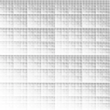
𝒮:{ϕ1(x,y)=(0.5x, 0.5y)ϕ2(x,y)=(0.5x+0.5, 0.5y)ϕ3(x,y)=(0.5x, 0.5y+0.5)ϕ4(x,y)=(0.5x+0.5, 0.5y+0.5):𝒮casessubscriptitalic-ϕ1𝑥𝑦absent0.5𝑥0.5𝑦subscriptitalic-ϕ2𝑥𝑦absent0.5𝑥0.50.5𝑦subscriptitalic-ϕ3𝑥𝑦absent0.5𝑥0.5𝑦0.5subscriptitalic-ϕ4𝑥𝑦absent0.5𝑥0.50.5𝑦0.5\mathcal{S}:\left\{\begin{array}[]{ll}\phi_{1}(x,y)&=(0.5x,\;0.5y)\\ \phi_{2}(x,y)&=(0.5x+0.5,\;0.5y)\\ \phi_{3}(x,y)&=(0.5x,\;0.5y+0.5)\\ \phi_{4}(x,y)&=(0.5x+0.5,\;0.5y+0.5)\\ \end{array}\right.

with the probabilities (p1=0.1,p2=0.2,p3=0.3,p4=0.4)formulae-sequencesubscript𝑝10.1formulae-sequencesubscript𝑝20.2formulae-sequencesubscript𝑝30.3subscript𝑝40.4(p_{1}=0.1,\;p_{2}=0.2,\;p_{3}=0.3,\;p_{4}=0.4). The comparison is made in Figure 1.

Refer to caption
Refer to caption
Figure 1: From the left to the right the output of the algorithm GIFSMeasureDraw(𝒮𝒮\mathcal{S}) after 8 iterations, with 512×512512512512\times 512 pixels and the picture IX.247 obtained in [Bar88] through a random process with 100.000 iterations.
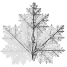
Example 5.6.

This example is a classic geometric fractal, the Maple Leaf. The approximation of the attractor by the algorithm IFSDraw(𝒮𝒮\mathcal{S}) from [dOS20] is presented in Figure 2 and the approximation of the discrete Hutchinson measure, through GIFSMeasureDraw(𝒮𝒮\mathcal{S}), is presented in the same figure. Consider X=[2,2]2𝑋superscript222X=[-2,2]^{2} and the IFS ϕ1,,ϕ4:XX:subscriptitalic-ϕ1subscriptitalic-ϕ4𝑋𝑋\phi_{1},...,\phi_{4}:X\to X with probabilities (pj)j=1L=4superscriptsubscriptsubscript𝑝𝑗𝑗1𝐿4(p_{j})_{j=1}^{L=4} where

𝒮:{ϕ1(x,y)=(0.8x+0.1,0.8y+0.04)ϕ2(x,y)=(0.5x+0.25,0.5y+0.4)ϕ3(x,y)=(0.355x0.355y+0.266,0.355x+0.355y+0.078)ϕ4(x,y)=(0.355x+0.355y+0.378,0.355x+0.355y+0.434):𝒮casessubscriptitalic-ϕ1𝑥𝑦absent0.8𝑥0.10.8𝑦0.04subscriptitalic-ϕ2𝑥𝑦absent0.5𝑥0.250.5𝑦0.4subscriptitalic-ϕ3𝑥𝑦absent0.355𝑥0.355𝑦0.2660.355𝑥0.355𝑦0.078subscriptitalic-ϕ4𝑥𝑦absent0.355𝑥0.355𝑦0.3780.355𝑥0.355𝑦0.434\mathcal{S}:\left\{\begin{array}[]{ll}\phi_{1}(x,y)&=(0.8x+0.1,0.8y+0.04)\\ \phi_{2}(x,y)&=(0.5x+0.25,0.5y+0.4)\\ \phi_{3}(x,y)&=(0.355x-0.355y+0.266,0.355x+0.355y+0.078)\\ \phi_{4}(x,y)&=(0.355x+0.355y+0.378,-0.355x+0.355y+0.434)\\ \end{array}\right.

As we can see, when the initial probabilities are small on the index of a map responsible for a part of the fractal attractor, the Hutchinson measure is very little concentrated on that part. For example, if we choose equal probability we will have a much more equal distribution as in Figure 3.
Refer to caption
Refer to caption
Refer to caption
Figure 2: From left to right, the output of the algorithm GIFSMeasureDraw(𝒮𝒮\mathcal{S}) after 5 iterations, 512×512512512512\times 512 pixels, with the set of probabilities (p1=0.3,p2=0.2,p3=0.05,p4=0.45)formulae-sequencesubscript𝑝10.3formulae-sequencesubscript𝑝20.2formulae-sequencesubscript𝑝30.05subscript𝑝40.45(p_{1}=0.3,\;p_{2}=0.2,\;p_{3}=0.05,\;p_{4}=0.45) and (p1=0.05,p2=0.2,p3=0.3,p4=0.45)formulae-sequencesubscript𝑝10.05formulae-sequencesubscript𝑝20.2formulae-sequencesubscript𝑝30.3subscript𝑝40.45(p_{1}=0.05,\;p_{2}=0.2,\;p_{3}=0.3,\;p_{4}=0.45) respectively, for the rightmost, algorithm IFSDraw(𝒮𝒮\mathcal{S}) after 12 iterations.
Refer to caption
Figure 3: The output of the algorithm GIFSMeasureDraw(𝒮𝒮\mathcal{S}) after 12 iterations, ε=0.004𝜀0.004\varepsilon=0.004 (512 points in a uniform net) with the set of probabilities (p1=0.25,p2=0.25,p3=0.25,p4=0.25)formulae-sequencesubscript𝑝10.25formulae-sequencesubscript𝑝20.25formulae-sequencesubscript𝑝30.25subscript𝑝40.25(p_{1}=0.25,\;p_{2}=0.25,\;p_{3}=0.25,\;p_{4}=0.25). In this case the measure ν𝜈\nu is a Hutchinson measure with resolution inferior to δ=0.2441701363𝛿0.2441701363\delta=0.2441701363.
Example 5.7.

This example is presented in the final section of [GMN16]. Each map consists of a translation followed by rotation and a dilation by a factor smaller than one, thus ensuring that it is a Banach contraction and hence our algorithm is applicable. The approximation of the discrete Hutchinson measure, through GIFSMeasureDraw(𝒮𝒮\mathcal{S}), is presented in the Figure 4. An approximation of the attractor, as a secondary output of the algorithm, is presented in Figure 5. Consider X=[0,1]2𝑋superscript012X=[0,1]^{2} and the IFS ϕ1,,ϕ4:XX:subscriptitalic-ϕ1subscriptitalic-ϕ4𝑋𝑋\phi_{1},...,\phi_{4}:X\to X with probabilities (pj)j=1L=4superscriptsubscriptsubscript𝑝𝑗𝑗1𝐿4(p_{j})_{j=1}^{L=4} where

𝒮:{ϕ1(x,y)=(cos(π6)(0.4x0.24)sin(π6)(0.4y0.08)+0.6,cos(π6)(0.4y0.08)+sin(π6)(0.4x0.24)+0.2)ϕ2(x,y)=(cos(π30)(0.6x0.03)+sin(π30)(0.6y0.12)+0.05,cos(π30)(0.6y0.12)sin(π30)(0.6x0.03)+0.2)ϕ3(x,y)=(0.5x0.475+0.95, 0.5y0.475+0.95)ϕ4(x,y)=(0.45x0.045+0.1, 0.45y0.405+0.9)\mathcal{S}:\left\{\begin{array}[]{ll}\phi_{1}(x,y)&=(\cos(\frac{\pi}{6})(0.4x-0.24)-\sin(\frac{\pi}{6})(0.4y-0.08)+0.6,\\ &\;\cos(\frac{\pi}{6})(0.4y-0.08)+\sin(\frac{\pi}{6})(0.4x-0.24)+0.2)\\ \phi_{2}(x,y)&=(\cos(\frac{\pi}{30})(0.6x-0.03)+\sin(\frac{\pi}{30})(0.6y-0.12)+0.05,\\ &\;\cos(\frac{\pi}{30})(0.6y-0.12)-\sin(\frac{\pi}{30})(0.6x-0.03)+0.2)\\ \phi_{3}(x,y)&=(0.5x-0.475+0.95,\;0.5y-0.475+0.95)\\ \phi_{4}(x,y)&=(0.45x-0.045+0.1,\;0.45y-0.405+0.9)\\ \end{array}\right.

and (p1=0.18,p2=0.22,p3=0.3,p4=3)formulae-sequencesubscript𝑝10.18formulae-sequencesubscript𝑝20.22formulae-sequencesubscript𝑝30.3subscript𝑝43(p_{1}=0.18,\;p_{2}=0.22,\;p_{3}=0.3,\;p_{4}=3).
As the maps are affine, a simple evaluation shows that α𝒮=0.6subscript𝛼𝒮0.6\alpha_{\mathcal{S}}=0.6, where 𝒮=(X,(ϕj)j=14,(pj)j=14)𝒮𝑋superscriptsubscriptsubscriptitalic-ϕ𝑗𝑗14superscriptsubscriptsubscript𝑝𝑗𝑗14\mathcal{S}=(X,(\phi_{j})_{j=1}^{4},(p_{j})_{j=1}^{4}) (α𝒮subscript𝛼𝒮\alpha_{\mathcal{S}} is the maximum contraction between the four maps ϕjsubscriptitalic-ϕ𝑗\phi_{j}, all being uniform contractions). After 15 iterations of our algorithm, which took only 5.56 seconds for 1024×1024102410241024\times 1024 pixels, we obtain (Figure 4, top-right) the associated Hutchinson (invariant) measure with resolution at most δ𝛿\delta, where δε1α𝒮+α𝒮ND=0.00310635similar-to𝛿𝜀1subscript𝛼𝒮superscriptsubscript𝛼𝒮𝑁𝐷0.00310635\delta\sim\frac{\varepsilon}{1-\alpha_{\mathcal{S}}}+\alpha_{\mathcal{S}}^{N}\,D=0.00310635, for N=15𝑁15N=15, ε=11024𝜀11024\varepsilon=\frac{1}{1024} and D=2𝐷2D=\sqrt{2}. Following the technique of [GMN16] a similar approximation (Figure 4, bottom) is given with resolution of at most 0.00475830.00475830.0047583, to compare. Most specifically, we have the following benchmark data given in the below table:

Pixels M×M𝑀𝑀M\times M Iter. Number N𝑁N Time(in seconds) Resol. at most δε1α𝒮+α𝒮NDsimilar-to𝛿𝜀1subscript𝛼𝒮superscriptsubscript𝛼𝒮𝑁𝐷\delta\sim\frac{\varepsilon}{1-\alpha_{\mathcal{S}}}+\alpha_{\mathcal{S}}^{N}\,D
256×256256256256\times 256 15 0.56 0.010430566982011563
512×512512512512\times 512 15 1.76 0.005547754482011564
1024×1024102410241024\times 1024 15 5.56 0.003106348232011563
Refer to caption
Refer to caption
Refer to caption
Refer to caption
Figure 4: From left to right, the output of the algorithm GIFSMeasureDraw(𝒮𝒮\mathcal{S}) after 15 iterations, for 256×256256256256\times 256, 512×512512512512\times 512 and 1024×1024102410241024\times 1024 pixels, with the prescribed set of probabilities; below, the picture given in [GMN16].
Refer to caption
Figure 5: The attractor A𝒮subscript𝐴𝒮A_{\mathcal{S}}, as the secondary output of the algorithm GIFSMeasureDraw(𝒮𝒮\mathcal{S}), for the same configurations as in Figure 4.

5.5 GIFS examples

Example 5.8.

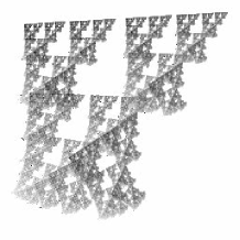
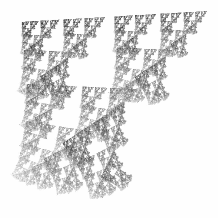
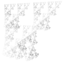
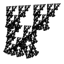
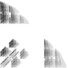
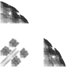
The approximation of the attractor by the algorithm GIFSDraw(𝒮𝒮\mathcal{S}) from [dOS20] is presented in Figure 6 and the approximation of the discrete Hutchinson measure, through GIFSMeasureDraw(𝒮𝒮\mathcal{S}), is presented in the same figure. Consider X=[0,1]2𝑋superscript012X=[0,1]^{2} and the GIFS ϕ1,,ϕ3:X2X:subscriptitalic-ϕ1subscriptitalic-ϕ3superscript𝑋2𝑋\phi_{1},...,\phi_{3}:X^{2}\to X with probabilities (pj)j=1L=3superscriptsubscriptsubscript𝑝𝑗𝑗1𝐿3(p_{j})_{j=1}^{L=3} where

𝒮:{ϕ1(x1,y1,x2,y2)=(0.25x1+0.2y2,0.25y1+0.2y2)ϕ2(x1,y1,x2,y2)=(0.25x1+0.2x2,0.25y1+0.1y2+0.5)ϕ3(x1,y1,x2,y2)=(0.25x1+0.1x2+0.5,0.25y1+0.2y2))\mathcal{S}:\left\{\begin{array}[]{ll}\phi_{1}(x_{1},y_{1},x_{2},y_{2})&=(0.25x_{1}+0.2y_{2},0.25y_{1}+0.2y_{2})\\ \phi_{2}(x_{1},y_{1},x_{2},y_{2})&=(0.25x_{1}+0.2x_{2},0.25y_{1}+0.1y_{2}+0.5)\\ \phi_{3}(x_{1},y_{1},x_{2},y_{2})&=(0.25x_{1}+0.1x_{2}+0.5,0.25y_{1}+0.2y_{2}))\\ \end{array}\right.

Once again, we can see that when the initial probabilities are small on the index of a map responsible for a part of the fractal attractor, the Hutchinson measure is very little concentrated on that part.
Refer to caption
Refer to caption
Refer to caption
Refer to caption
Figure 6: On the top, from the left to the right the output of the algorithm GIFSMeasureDraw(𝒮𝒮\mathcal{S}) after 12 iterations, with the set of probabilities (p1=0.10,p2=0.45,p3=0.45)formulae-sequencesubscript𝑝10.10formulae-sequencesubscript𝑝20.45subscript𝑝30.45(p_{1}=0.10,\;p_{2}=0.45,\;p_{3}=0.45), (p1=0.45,p2=0.10,p3=0.45)formulae-sequencesubscript𝑝10.45formulae-sequencesubscript𝑝20.10subscript𝑝30.45(p_{1}=0.45,\;p_{2}=0.10,\;p_{3}=0.45) and (p1=0.45,p2=0.45,p3=0.10)formulae-sequencesubscript𝑝10.45formulae-sequencesubscript𝑝20.45subscript𝑝30.10(p_{1}=0.45,\;p_{2}=0.45,\;p_{3}=0.10) respectively. On the bottom, algorithm GIFSDraw(𝒮𝒮\mathcal{S}) after 12 iterations. In all the cases we have , 512×512512512512\times 512 pixels.

6 Further applications

6.1 Approximating integrals with respect to stationary Probability measures

In a recent preprint [CJ19] the authors describe a method to approximate integral of functions with respect to stationary probability measures (measures that are fixed points for the Markov operator associated to an IFS with probabilities, M𝒮(μ𝒮)=μ𝒮subscript𝑀𝒮subscript𝜇𝒮subscript𝜇𝒮M_{\mathcal{S}}\left(\mu_{\mathcal{S}}\right)=\mu_{\mathcal{S}}) which are the Hutchinson measures for those IFSs. The setting is the interval [0,1]01[0,1] and the IFS is required to fulfill some additional regularity properties such as holomorphic extension, control of derivatives of the maps in the IFS and on the set of functions that one may integrate.

Since our algorithm GIFSMeasureDraw(𝒮𝒮\mathcal{S}) for dimension 111 provides a discrete δ𝛿\delta-approximation of such measures μ𝒮subscript𝜇𝒮\mu_{\mathcal{S}} in the form

ν:=k=1nνikδx[ik]assign𝜈superscriptsubscript𝑘1𝑛subscript𝜈subscript𝑖𝑘subscript𝛿𝑥delimited-[]subscript𝑖𝑘\nu:=\sum_{k=1}^{n}\nu_{i_{k}}\delta_{x[i_{k}]}

where the points x[ik]𝑥delimited-[]subscript𝑖𝑘x[i_{k}] are in the correspondent δ𝛿\delta-approximation of the actual attractor, we can approximate the integral of a Lipschitz function g:[0,1]:𝑔01g:[0,1]\to\mathbb{R} by

[0,1]g𝑑μ𝒮k=1nνikg(x[ik])similar-to-or-equalssubscript01𝑔differential-dsubscript𝜇𝒮superscriptsubscript𝑘1𝑛subscript𝜈subscript𝑖𝑘𝑔𝑥delimited-[]subscript𝑖𝑘\int_{[0,1]}gd\mu_{\mathcal{S}}\simeq\sum_{k=1}^{n}\nu_{i_{k}}g(x[i_{k}])

with precision δ𝛿\delta.

As a demonstration of this we next describe the measures and the integrals for three examples found in [CJ19] using our algorithms.

Example 6.1.

In this first example we consider the Hausdorff moment of the Hutchinson measure μ𝒮subscript𝜇𝒮\mu_{\mathcal{S}} which is given by

γn=γn(μ𝒮):=xndμ𝒮(x),n=0,1,formulae-sequencesubscript𝛾𝑛subscript𝛾𝑛subscript𝜇𝒮assignsuperscriptsubscriptsuperscript𝑥𝑛differential-dsubscript𝜇𝒮𝑥𝑛01\gamma_{n}=\gamma_{n}(\mu_{\mathcal{S}}):=\int_{-\infty}^{\infty}x^{n}\mathrm{d}\mu_{\mathcal{S}}(x),n=0,1,\ldots
𝒮:{ϕ1(x)=13xϕ2(x)=13x+23:𝒮casessubscriptitalic-ϕ1𝑥absent13𝑥subscriptitalic-ϕ2𝑥absent13𝑥23\mathcal{S}:\left\{\begin{array}[]{ll}\phi_{1}(x)&=\frac{1}{3}x\\ \phi_{2}(x)&=\frac{1}{3}x+\frac{2}{3}\\ \end{array}\right.

with probabilities p1:=1/3assignsubscript𝑝113p_{1}:=1/3 and p2:=2/3assignsubscript𝑝223p_{2}:=2/3.

For purpose of comparison we use the algorithm GIFSMeasureDraw(𝒮𝒮\mathcal{S}) to approximate μ𝒮subscript𝜇𝒮\mu_{\mathcal{S}} (see Figure 7) and then compute γn,n=0,1,,10formulae-sequencesubscript𝛾𝑛𝑛0110\gamma_{n},n=0,1,\ldots,10:

Refer to caption
Figure 7: Histogram of μ𝒮subscript𝜇𝒮\mu_{\mathcal{S}} produced by algorithm GIFSMeasureDraw(𝒮𝒮\mathcal{S}) with resolution δ=0.0001𝛿0.0001\delta=0.0001 after 10 iterations, having a high definition 50,0005000050,000 pixels taking 1.9 seconds.

The first 101010 moments are displayed in Table 1.

n𝑛n Approx. k=1mνik(x[ik])nsuperscriptsubscript𝑘1𝑚subscript𝜈subscript𝑖𝑘superscript𝑥delimited-[]subscript𝑖𝑘𝑛\sum_{k=1}^{m}\nu_{i_{k}}(x[i_{k}])^{n} Actual value [0,1]xn𝑑μ𝒮subscript01superscript𝑥𝑛differential-dsubscript𝜇𝒮\int_{[0,1]}x^{n}d\mu_{\mathcal{S}}, from [CJ19].
0 1.0000000 1
1 0.6666608 2/3=0.66666666666…
2 0.5555478 5/9=0.55555555555…
3 0.4957168 58/117=0.49572649572…
4 0.4552590 799/1755=0.45527065527…
5 0.4246685
6 0.4002248
7 0.3800868
8 0.3631560 1213077397297/3340208879865=0.36317411303…
9 0.3486940 764170684622650/2191399705783431=0.34871351064…
10 0.3361713 16313445679660723325/48524163685162512633=0.33619220694…
Table 1: Moments using the δ𝛿\delta-approximation of μ𝒮subscript𝜇𝒮\mu_{\mathcal{S}} by GIFSMeasureDraw(𝒮𝒮\mathcal{S})
Example 6.2.

In this second example we consider the Wasserstein distance between two Hutchinson measures μ𝒮1subscript𝜇subscript𝒮1\mu_{\mathcal{S}_{1}} and μ𝒮2subscript𝜇subscript𝒮2\mu_{\mathcal{S}_{2}} (see Figure 8) associated to different probabilities for the same IFS

𝒮:{ϕ1(x)=sin(πx/4)6+14ϕ2(x)=sin(πx/4)3+23:𝒮casessubscriptitalic-ϕ1𝑥absent𝜋𝑥4614subscriptitalic-ϕ2𝑥absent𝜋𝑥4323\mathcal{S}:\left\{\begin{array}[]{ll}\phi_{1}(x)&=\frac{\sin(\pi x/4)}{6}+\frac{1}{4}\\ \phi_{2}(x)&=\frac{\sin(\pi x/4)}{3}+\frac{2}{3}\\ \end{array}\right.

with probabilities p1:=1/7,p2:=6/7formulae-sequenceassignsubscript𝑝117assignsubscript𝑝267p_{1}:=1/7,p_{2}:=6/7 and q1:=1/2,q2:=1/2formulae-sequenceassignsubscript𝑞112assignsubscript𝑞212q_{1}:=1/2,q_{2}:=1/2 respectively.

It is easy to see that the IFS is π12𝜋12\frac{\pi}{12}-Lipschitz. Then our algorithm GIFSMeasureDraw(𝒮𝒮\mathcal{S}) can be used to approximate the integrals and, in particular, under the hypothesis of [CJ19] the Wasserstein distance is given by

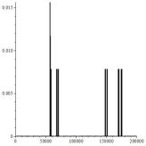
W1(μ𝒮1,μ𝒮2)=|xdμ𝒮2xdμ𝒮1|0.22104594557263850324subscript𝑊1subscript𝜇subscript𝒮1subscript𝜇subscript𝒮2𝑥differential-dsubscript𝜇subscript𝒮2𝑥differential-dsubscript𝜇subscript𝒮1similar-to-or-equals0.22104594557263850324W_{1}\left(\mu_{\mathcal{S}_{1}},\mu_{\mathcal{S}_{2}}\right)=\left|\int x\mathrm{d}\mu_{\mathcal{S}_{2}}-\int x\mathrm{d}\mu_{\mathcal{S}_{1}}\right|\simeq 0.22104594557263850324...
Refer to caption
Refer to caption
Figure 8: From left to right: the histograms of μ𝒮1subscript𝜇subscript𝒮1\mu_{\mathcal{S}_{1}} and μ𝒮2subscript𝜇subscript𝒮2\mu_{\mathcal{S}_{2}} produced by algorithm GIFSMeasureDraw(𝒮𝒮\mathcal{S}) with resolution δ=0.00003𝛿0.00003\delta=0.00003 after 10 iterations, having a high definition 200,000200000200,000 pixels taking 5.8 seconds.
Example 6.3.

For the last, we consider the problem of compute the Lyapunov exponent of the Hutchinson measure μ𝒮subscript𝜇𝒮\mu_{\mathcal{S}} (see Figure 9) of a IFSp given by

χμ𝒮:=i=12pilog|ϕi(x)|dμ𝒮(x)1.7367208099326368assignsubscript𝜒subscript𝜇𝒮superscriptsubscript𝑖12subscript𝑝𝑖superscriptsubscriptitalic-ϕ𝑖𝑥dsubscript𝜇𝒮𝑥similar-to-or-equals1.7367208099326368\chi_{\mu_{\mathcal{S}}}:=-\int\sum_{i=1}^{2}p_{i}\log\left|\phi_{i}^{\prime}(x)\right|\mathrm{d}\mu_{\mathcal{S}}(x)\simeq 1.7367208099326368...

for

𝒮:{ϕ1(x)=sin(πx/4)6+14ϕ2(x)=sin(πx/4)3+23:𝒮casessubscriptitalic-ϕ1𝑥absent𝜋𝑥4614subscriptitalic-ϕ2𝑥absent𝜋𝑥4323\mathcal{S}:\left\{\begin{array}[]{ll}\phi_{1}(x)&=\frac{\sin(\pi x/4)}{6}+\frac{1}{4}\\ \phi_{2}(x)&=\frac{\sin(\pi x/4)}{3}+\frac{2}{3}\\ \end{array}\right.

with probabilities p1:=1/3,p2:=2/3formulae-sequenceassignsubscript𝑝113assignsubscript𝑝223p_{1}:=1/3,p_{2}:=2/3.

Refer to caption
Figure 9: The histogram of μ𝒮subscript𝜇𝒮\mu_{\mathcal{S}} produced by algorithm GIFSMeasureDraw(𝒮𝒮\mathcal{S}) with resolution δ=2.11×10⁶𝛿2.11superscript106\delta=2.11\times 10^{-6} after 20 iterations, having a high definition 3,200,00032000003,200,000 pixels taking 0.5690 seconds.

6.2 Projected Hutchinson measures

One can easily adapt algorithm GIFSMeasureDraw(𝒮𝒮\mathcal{S}) to also compute the integral of a function with respect to the Hutchinson measure and compare this result against the typical averages, as predicted by Elton’s ergodic theorem, see [Elt87].

For example, given the GIFS 𝒮𝒮\mathcal{S} from [Oli17, Example 11],

𝒮:{ϕ1(x,y)=13x+14yϕ2(x,y)=13x14y+12:𝒮casessubscriptitalic-ϕ1𝑥𝑦absent13𝑥14𝑦subscriptitalic-ϕ2𝑥𝑦absent13𝑥14𝑦12\mathcal{S}:\left\{\begin{array}[]{ll}\phi_{1}(x,y)&=\frac{1}{3}x+\frac{1}{4}y\\ \phi_{2}(x,y)&=\frac{1}{3}x-\frac{1}{4}y+\frac{1}{2}\\ \end{array}\right.

we consider its extension

:{ψ1(x,y)=(y,13x+14y)ψ2(x,y)=(y,13x14y+12):casessubscript𝜓1𝑥𝑦absent𝑦13𝑥14𝑦subscript𝜓2𝑥𝑦absent𝑦13𝑥14𝑦12\mathcal{R}:\left\{\begin{array}[]{ll}\psi_{1}(x,y)&=(y,\frac{1}{3}x+\frac{1}{4}y)\\ \psi_{2}(x,y)&=(y,\frac{1}{3}x-\frac{1}{4}y+\frac{1}{2})\\ \end{array}\right.

which is an eventually contractive IFS on [0,1]2superscript012[0,1]^{2} (the second power of \mathcal{R} is 0.54355419040.54355419040.5435541904-Lipschtz), so our theory works. In both cases we consider probabilities p1:=0.65assignsubscript𝑝10.65p_{1}:=0.65 and p2:=0.35assignsubscript𝑝20.35p_{2}:=0.35. As pointed out in [Oli17], if ν𝒫([0,1])𝜈𝒫01\nu\in\mathcal{P}([0,1]) is the Hutchinson measure for the GIFSp 𝒮=(X,(ϕj)j=12,(pj)j=12)𝒮𝑋superscriptsubscriptsubscriptitalic-ϕ𝑗𝑗12superscriptsubscriptsubscript𝑝𝑗𝑗12\mathcal{S}=(X,(\phi_{j})_{j=1}^{2},(p_{j})_{j=1}^{2}) and μ𝒫([0,1]2)subscript𝜇𝒫superscript012\mu_{\mathcal{R}}\in\mathcal{P}([0,1]^{2}) is the Hutchinson measure for the IFSp =(X,(ψj)j=12,(pj)j=12)𝑋superscriptsubscriptsubscript𝜓𝑗𝑗12superscriptsubscriptsubscript𝑝𝑗𝑗12\mathcal{R}=(X,(\psi_{j})_{j=1}^{2},(p_{j})_{j=1}^{2}) (see Figure 10) then νν𝜈superscript𝜈\nu\neq\nu^{\prime}, where νsuperscript𝜈\nu^{\prime} is the projected Hutchinson measure Π1(μ)superscriptsubscriptΠ1subscript𝜇\Pi_{1}^{\sharp}(\mu_{\mathcal{R}}).

Using our algorithms we are capable to display a histogram representation of such distributions on [0,1]01[0,1]. In each case the height of each vertical bar represents the approximate measure of a cell in the ε𝜀\varepsilon-net with 350350350 points in X=[0,1]𝑋01X=[0,1], and resolution 2×10²²superscript1022\times 10^{-2} (see Figure 11).

Refer to caption
Refer to caption
Figure 10: The output of algorithm GIFSMeasureDraw(\mathcal{R}) after 25 iterations, having a fairly high definition, 512×512512512512\times 512 pixels. On the left the attractor Asubscript𝐴A_{\mathcal{R}} on the right the histogram of μsubscript𝜇\mu_{\mathcal{R}}.
Refer to caption
Refer to caption
Figure 11: The output of algorithm GIFSMeasureDraw(𝒮𝒮\mathcal{S}) after 25 iterations, having a fairly high definition 350×350350350350\times 350 pixels. On the left the attractor ν𝜈\nu on the right the histogram of ν=Π1(μ)superscript𝜈superscriptsubscriptΠ1subscript𝜇\nu^{\prime}=\Pi_{1}^{\sharp}(\mu_{\mathcal{R}}) which is the projection of the Figure 10.

The ergodic theorem for projected Hutchinson measures from [Oli17] claims that

limN+1Nn=0N1f(xn(a))=Xf(t)𝑑ν(t)subscript𝑁1𝑁superscriptsubscript𝑛0𝑁1𝑓subscript𝑥𝑛𝑎subscript𝑋𝑓𝑡differential-dsuperscript𝜈𝑡\lim_{N\rightarrow+\infty}\frac{1}{N}\sum_{n=0}^{N-1}f\left(x_{n}(a)\right)=\int_{X}f(t)d\nu^{\prime}(t)

where xn(a)subscript𝑥𝑛𝑎x_{n}(a) is the projection on the first coordinate and a𝑎a is a sequence of symbols chosen with probability one in the sequences of {1,2}superscript12\{1,2\}^{\mathbb{N}} according to the probabilities p1:=0.65assignsubscript𝑝10.65p_{1}:=0.65 and p2:=0.35assignsubscript𝑝20.35p_{2}:=0.35.

Consider f(x)=x2𝑓𝑥superscript𝑥2f(x)=x^{2}: using the measure obtained by GIFSMeasureDraw(\mathcal{R}) for estimate 01x2𝑑ν(x)superscriptsubscript01superscript𝑥2differential-dsuperscript𝜈𝑥\int_{0}^{1}x^{2}d\nu^{\prime}(x), the projected measure, we obtain

01x2𝑑ν(x)0.12177521930similar-to-or-equalssuperscriptsubscript01superscript𝑥2differential-dsuperscript𝜈𝑥0.12177521930\int_{0}^{1}x^{2}d\nu^{\prime}(x)\,\simeq 0.12177521930...

On the other hand, using the ergodic theorem where each aisubscript𝑎𝑖a_{i} in the sequence a=(a0,a1,a2,)𝑎subscript𝑎0subscript𝑎1subscript𝑎2a=(a_{0},a_{1},a_{2},...) is picked from a random i.i.d.ṽariable I{1,2}𝐼12I\in\{1,2\} with distribution p1:=0.65assignsubscript𝑝10.65p_{1}:=0.65 and p2:=0.35assignsubscript𝑝20.35p_{2}:=0.35, x0=0.5subscript𝑥00.5x_{0}=0.5 and N=10.000𝑁10.000N=10.000 we get

110000n=0100001(xn(a))20.1228183842857similar-to-or-equals110000superscriptsubscript𝑛0100001superscriptsubscript𝑥𝑛𝑎20.1228183842857\frac{1}{10000}\sum_{n=0}^{10000-1}\left(x_{n}(a)\right)^{2}\,\simeq 0.1228183842857\ldots

with an absolute error of 5×1025superscript1025\times 10^{-2}. For a fractal computed on a resolution of 500×500500500500\times 500 pixels the error is 3×1043superscript1043\times 10^{-4}.

6.3 IFS and GIFS with place dependent probabilities

We consider variable probabilities, that is, each pjsubscript𝑝𝑗p_{j} is as function of x𝑥x, such as in [Hut81], [BDEG88, Theorem 2.1], assuming average-contractiveness, [Ste02], [Öbe05] and more recently [GMM19] for IFS and in [Mic14, Section 3] for GIFS.

We notice that Lemma 4.2 is still valid under the variable probability hypothesis. Thus we just need to ensure that the respective Markov operator is Banach contractive to use Theorem 3.2. We are not going to remake several straightforward computations to update the algorithms. We only update the necessary computation of the probabilities in each case (both in the bidimensional version):

  • In the algorithm GIFSMeasureDraw(𝒮𝒮\mathcal{S}) we replace

    ν(x1[i1],,xd[id]):=ν(x1[i1],,xd[id])+pjνy0νym1assignsubscript𝜈subscript𝑥1delimited-[]superscript𝑖1subscript𝑥𝑑delimited-[]superscript𝑖𝑑subscript𝜈subscript𝑥1delimited-[]superscript𝑖1subscript𝑥𝑑delimited-[]superscript𝑖𝑑subscript𝑝𝑗subscript𝜈subscript𝑦0subscript𝜈subscript𝑦𝑚1\nu_{(x_{1}[i^{1}],...,x_{d}[i^{d}])}:=\nu_{(x_{1}[i^{1}],...,x_{d}[i^{d}])}+p_{j}\nu_{y_{0}}\cdot...\cdot\nu_{y_{m-1}}

    by

    ν(x1[i1],,xd[id]):=ν(x1[i1],,xd[id])+pj(y0,..,ym1)νy0νym1\nu_{(x_{1}[i^{1}],...,x_{d}[i^{d}])}:=\nu_{(x_{1}[i^{1}],...,x_{d}[i^{d}])}+p_{j}(y_{0},..,y_{m-1})\nu_{y_{0}}\cdot...\cdot\nu_{y_{m-1}}
Example 6.4.

In [Mih08, p. 146], the author considers the one dimensional case X=[0,1]𝑋01X=[0,1] and a GIFS 𝒮=(X,(ϕj)j=12)𝒮𝑋superscriptsubscriptsubscriptitalic-ϕ𝑗𝑗12\mathcal{S}=(X,(\phi_{j})_{j=1}^{2}) where

{ϕ1(x,y)=x4+y4ϕ2(x,y)=x4+y4+12.casessubscriptitalic-ϕ1𝑥𝑦absent𝑥4𝑦4subscriptitalic-ϕ2𝑥𝑦absent𝑥4𝑦412\left\{\begin{array}[]{ll}\phi_{1}(x,y)=&\frac{x}{4}+\frac{y}{4}\\ \phi_{2}(x,y)=&\frac{x}{4}+\frac{y}{4}+\frac{1}{2}.\end{array}\right.

Given a function

α(t)={1, if t[0,14]24t, if t[14,12]0, if t[12,1]𝛼𝑡cases1 if 𝑡01424𝑡 if 𝑡14120 if 𝑡121\alpha(t)=\left\{\begin{array}[]{ll}{1,}&{\text{ if }t\in\left[0,\frac{1}{4}\right]}\\ {2-4t,}&{\text{ if }t\in\left[\frac{1}{4},\frac{1}{2}\right]}\\ {0,}&{\text{ if }t\in\left[\frac{1}{2},1\right]}\end{array}\right.

he considers the probabilities p1(x,y)=133α(x)α(y)subscript𝑝1𝑥𝑦133𝛼𝑥𝛼𝑦p_{1}(x,y)=\frac{1}{33}\alpha(x)\alpha(y),

p2(x,y)=1p1(x,y)=1133α(x)α(y),subscript𝑝2𝑥𝑦1subscript𝑝1𝑥𝑦1133𝛼𝑥𝛼𝑦p_{2}(x,y)=1-p_{1}(x,y)=1-\frac{1}{33}\alpha(x)\alpha(y),

and the GIFSpdp 𝒮=(X,(ϕj)j=12,(pj)j=12)𝒮𝑋superscriptsubscriptsubscriptitalic-ϕ𝑗𝑗12superscriptsubscriptsubscript𝑝𝑗𝑗12\mathcal{S}=(X,(\phi_{j})_{j=1}^{2},(p_{j})_{j=1}^{2}).

Under this hypothesis, he verifies that M𝒮subscript𝑀𝒮M_{\mathcal{S}} is a contraction and μ𝒮subscript𝜇𝒮\mu_{\mathcal{S}} is its only fixed point. More than that, he verifies that the attractor is A𝒮=[0,1]subscript𝐴𝒮01A_{\mathcal{S}}=[0,1] and suppμ𝒮[0,14][12,1]suppsubscript𝜇𝒮014121\mathop{\rm supp}\nolimits\mu_{\mathcal{S}}\subseteq\left[0,\frac{1}{4}\right]\cup\left[\frac{1}{2},1\right].

From the previous discussion it is easy to see that our algorithm GIFSMeasureDraw(𝒮𝒮\mathcal{S}) can be used to get approximations of μ𝒮subscript𝜇𝒮\mu_{\mathcal{S}} as we can see in figure 12

Refer to caption
Refer to caption
Refer to caption
Figure 12: The output of the algorithm GIFSMeasureDraw(𝒮𝒮\mathcal{S}) after 1, 5 and 15 iterations, having a fairly high definition of 300300300 pixels.

The output suggests that μ𝒮=δ1subscript𝜇𝒮subscript𝛿1\mu_{\mathcal{S}}=\delta_{1}! We can verify that by direct examination as follows.

Consider a continuous function f:[0,1]:𝑓01f:[0,1]\to\mathbb{R} then,

f(z)𝑑M𝒮(δ1×δ1)=xyp1(x,y)f(ϕ1(x,y))+p2(x,y)f(ϕ1(x,y))dδ1(x)dδ1(y)=𝑓𝑧differential-dsubscript𝑀𝒮subscript𝛿1subscript𝛿1subscript𝑥subscript𝑦subscript𝑝1𝑥𝑦𝑓subscriptitalic-ϕ1𝑥𝑦subscript𝑝2𝑥𝑦𝑓subscriptitalic-ϕ1𝑥𝑦𝑑subscript𝛿1𝑥𝑑subscript𝛿1𝑦absent\int f(z)dM_{\mathcal{S}}(\delta_{1}\times\delta_{1})=\int_{x}\int_{y}p_{1}(x,y)f(\phi_{1}(x,y))+p_{2}(x,y)f(\phi_{1}(x,y))d\delta_{1}(x)d\delta_{1}(y)=
=p1(1,1)f(ϕ1(1,1))+p2(1,1)f(ϕ1(1,1))=p1(1,1)f(14+14)+p2(1,1)f(14+14+12)=absentsubscript𝑝111𝑓subscriptitalic-ϕ111subscript𝑝211𝑓subscriptitalic-ϕ111subscript𝑝111𝑓1414subscript𝑝211𝑓141412absent=p_{1}(1,1)f(\phi_{1}(1,1))+p_{2}(1,1)f(\phi_{1}(1,1))=p_{1}(1,1)f\left(\frac{1}{4}+\frac{1}{4}\right)+p_{2}(1,1)f\left(\frac{1}{4}+\frac{1}{4}+\frac{1}{2}\right)=
=f(1)=f(z)dδ1(z)),=f(1)=\int f(z)d\delta_{1}(z)),

because p1(1,1)=0subscript𝑝1110p_{1}(1,1)=0. Therefore, M𝒮(δ1×δ1)=δ1subscript𝑀𝒮subscript𝛿1subscript𝛿1subscript𝛿1M_{\mathcal{S}}(\delta_{1}\times\delta_{1})=\delta_{1} meaning that μ𝒮=δ1subscript𝜇𝒮subscript𝛿1\mu_{\mathcal{S}}=\delta_{1}.

Example 6.5.

In this case we consider a negative case from [CR90]. In this case the authors consider the doubling map T(x)=2xmod1𝑇𝑥modulo2𝑥1T(x)=2x\mod 1 on the interval and studies the solutions of the equation

Puf(x)=u(x2)f(x2)+u(x2+12)f(x2+12)subscript𝑃𝑢𝑓𝑥𝑢𝑥2𝑓𝑥2𝑢𝑥212𝑓𝑥212P_{u}f(x)=u\left(\frac{x}{2}\right)f\left(\frac{x}{2}\right)+u\left(\frac{x}{2}+\frac{1}{2}\right)f\left(\frac{x}{2}+\frac{1}{2}\right)

for a given potential u:[0,1]:𝑢01u:[0,1]\to\mathbb{R} and the Pusubscript𝑃𝑢P_{u}-harmonic functions, i. e. Pu(f)=fsubscript𝑃𝑢𝑓𝑓P_{u}(f)=f. Then they characterizes the dual solutions Pu(μ)=μsuperscriptsubscript𝑃𝑢𝜇𝜇P_{u}^{*}(\mu)=\mu, which he calls invariant measures.

It follows that this problem is the same as the problem of finding the Hutchinson measure for the IFSpdp 𝒮=(X,(ϕj)j=12,(pj)j=12)𝒮𝑋superscriptsubscriptsubscriptitalic-ϕ𝑗𝑗12superscriptsubscriptsubscript𝑝𝑗𝑗12\mathcal{S}=(X,(\phi_{j})_{j=1}^{2},(p_{j})_{j=1}^{2}) where

{ϕ1(x)=x2ϕ2(x)=x2+12.casessubscriptitalic-ϕ1𝑥absent𝑥2subscriptitalic-ϕ2𝑥absent𝑥212\left\{\begin{array}[]{ll}\phi_{1}(x)=&\frac{x}{2}\\ \phi_{2}(x)=&\frac{x}{2}+\frac{1}{2}.\end{array}\right.

Given a function, say u(t)=cos2(3πt)𝑢𝑡superscript23𝜋𝑡u(t)=\cos^{2}(3\pi t), there are considered probabilities p1(x)=u(ϕ1(x))=u(x/2)subscript𝑝1𝑥𝑢subscriptitalic-ϕ1𝑥𝑢𝑥2p_{1}(x)=u(\phi_{1}(x))=u(x/2) and p2(x)=u(ϕ2(x))=u(x/2+1/2)subscript𝑝2𝑥𝑢subscriptitalic-ϕ2𝑥𝑢𝑥212p_{2}(x)=u(\phi_{2}(x))=u(x/2+1/2).

Refer to caption Refer to caption
Figure 13: The output of algorithm GIFSMeasureDraw(𝒮𝒮\mathcal{S}) after 1 and 100 iterations, having a fairly high definition of 500500500 pixels. In the first row, after 100100100 iterations the discrete measure is μ:=0.1030321845δ0+0.8199775187δ13+0.06209698542δ23+0.01471437940δ1assign𝜇0.1030321845subscript𝛿00.8199775187subscript𝛿130.06209698542subscript𝛿230.01471437940subscript𝛿1\mu:=0.1030321845\,\delta_{0}+0.8199775187\,\delta_{\frac{1}{3}}+0.06209698542\,\delta_{\frac{2}{3}}+0.01471437940\,\delta_{1}; in the second row, after 100100100 iterations the discrete measure is μ:=0.05792616463δ0+0.4568641232δ13+0.4317603436δ23+0.05323785154δ1assign𝜇0.05792616463subscript𝛿00.4568641232subscript𝛿130.4317603436subscript𝛿230.05323785154subscript𝛿1\mu:=0.05792616463\,\delta_{0}+0.4568641232\,\delta_{\frac{1}{3}}+0.4317603436\,\delta_{\frac{2}{3}}+0.05323785154\,\delta_{1}.

In [CR90, example 3 b], the authors show that the invariant measures (Hutchinson measures for the IFSpdp) are the probabilities supported on the T𝑇T-periodic cycles {0}0\{0\}, {1}1\{1\} and {13,23}1323\{\frac{1}{3},\frac{2}{3}\}. In that case our Markov operator cannot be a contraction because there is more than one Hutchinson measure; however, we can still use GIFSMeasureDraw(𝒮𝒮\mathcal{S}) to see if it converges to any measure. We show in Figure 13 a selection phenomenon: the iteration seems to converge to some combination μ:=aδ0+bδ13+cδ23+dδ1assign𝜇𝑎subscript𝛿0𝑏subscript𝛿13𝑐subscript𝛿23𝑑subscript𝛿1\mu:=a\delta_{0}+b\delta_{\frac{1}{3}}+c\delta_{\frac{2}{3}}+d\delta_{1} depending on the initial measure we choose.

Acknowledgments

We are grateful to the referees whose careful reading improved the paper.

References

  • [Bar88] M.F. Barnsley. Fractals Everywhere. Academic Press, Inc., Boston, MA, 1988.
  • [BDEG88] M.F. Barnsley, S.G. Demko, J.H. Elton, and J. S. Geronimo. Invariant measures for Markov processes arising from iterated function systems with place-dependent probabilities. Ann. Inst. H. Poincaré Probab. Statist., 24(3):367–394, 1988.
  • [Bla01] M. Blank. Perron-Frobenius spectrum for random maps and its approximation. Moscow Mathematical Journal, 1(3):315–344, 2001.
  • [Bog07] V. Bogachev. Measure Theory. Springer, Springer-Verlag, Berlin, 2007.
  • [BP13] V. Berinde and M. Pacurar. The role of the Pompeiou-Hausdorff metric in fixed point theory. Creative Mathematics and Informatics, 22(13):143–150, 2013.
  • [CJ19] I. Cipriano and N. Jurga. Approximating integrals with respect to stationary probability measures of iterated function systems. Preprint https://arxiv.org/abs/1907.03872, 2019.
  • [CR90] J.P. Conze and A. Raugi. Fonctions harmoniques pour un opérateur de transition et applications. Bulletin Societé Mathematique de France, 118(3):273–210, 1990.
  • [dOS20] R.D. da Cunha, E.R. Oliveira, and F. Strobin. A multiresolution algorithm to generate images of generalized fuzzy fractal attractors. https://doi.org/10.1007/s11075-020-00886-w, 2020.
  • [Elt87] E.J. Elton. An ergodic theorem for iterated maps. Ergodic Theory and Dynamical Systems, 7(4):481–488, 1987.
  • [Fro99] G. Froyland. Ulam’s method for random interval maps. Nonlinearity, 12(4):1029–1051, January 1999.
  • [GMM19] F. Georgescu, R. Miculescu, and A. Mihail. Invariant measures of Markov operators associated to iterated function systems consisting of ϕitalic-ϕ\phi-max-contractions with probabilities. Indagationes Mathematicae, 30(1):214–226, 2019.
  • [GMN16] S. Galatolo, M. Monge, and I. Nisoli. Rigorous approximation of stationary measures and convergence to equilibrium for iterated function systems. Journal of Physics A: Mathematical and Theoretical, 49(27):274001, May 2016.
  • [GN14] S. Galatolo and I. Nisoli. An elementary approach to rigorous approximation of invariant measures. SIAM Journal on Applied Dynamical Systems, 13(2):958–985, 2014.
  • [Hut81] J. Hutchinson. Fractals and self-similarity. Indiana University Mathematics Journal, 30(5):713–747, 1981.
  • [JMS16] P. Jaros, Ł. Maślanka, and F. Strobin. Algorithms generating images of attractors of generalized iterated function systems. Numerical Algorithms, 73(2):477–499, October 2016.
  • [JP07] O. Jenkinson and M. Pollicott. A dynamical approach to accelerating numerical integration with equidistributed points. Proceedings of the Steklov Institute of Mathematics, 256(1):275–289, April 2007.
  • [KLMV12] H. Kunze, D. La Torre, F. Mendivil, and E.R. Vrscay. Fractal-Based Methods in Analysis. Springer, Springer US, 2012.
  • [Mic14] R. Miculescu. Generalized iterated function systems with place dependent probabilities. Acta Applicandae Mathematicae, 130(1):135–150, April 2014.
  • [Mih08] A. Mihail. Recurrent iterated function systems. Revue Roumaine de Mathématiques Pures et Appliqués, 53(1):43–53, 2008.
  • [Mih09] A. Mihail. The Hutchinson measure for generalized iterated function systems. Revue Roumaine de Mathématiques Pures et Appliqués, 54(4):297–316, 2009.
  • [MM08] A. Mihail and R. Miculescu. Applications of fixed point theorems in the theory of generalized ifs. Fixed Point Theory and Applications, 2008(1):312876, May 2008.
  • [MM09] Alexandru Mihail and Radu Miculescu. A generalization of the hutchinson measure. Mediterranean Journal of Mathematics, 6(2):203–213, July 2009.
  • [MM10] A. Mihail and R. Miculescu. Generalized ifss on noncompact spaces. Fixed Point Theory and Applications, 2010(1):584215, January 2010.
  • [MMU20] R. Miculescu, A. Mihail, and S.-A. Urziceanu. A new algorithm that generates the image of the attractor of a generalized iterated function system. Numerical Algorithms, 83(4):1399–1413, April 2020.
  • [MS19] Ł. Maślanka and F. Strobin. Zero-dimensional compact metrizable spaces as attractors of generalized iterated function systems. Topological Methods in Nonlinear Analysis, 53(1):363–403, March 2019.
  • [Öbe05] A. Öberg. Algorithms for approximation of invariant measures for ifs. Manuscripta Mathematica, 116(1):31–55, January 2005.
  • [Öbe06] A. Öberg. Approximation of invariant measures for random iterations. Rocky Mountain J. Math., 36(1):273–301, 02 2006.
  • [Oli17] E.R. Oliveira. The ergodic theorem for a new kind of attractor of a gifs. Chaos, Solitons & Fractals, 98:63–71, May 2017.
  • [SS13] F. Strobin and Jarosław Swaczyna. On a certain generalisation of the iterated function system. Bulletin of the Australian Mathematical Society, 87(1):37–54, 2013.
  • [Ste02] Ö. Stenflo. Uniqueness of invariant measures for place-dependent random iterations of functions, volume 132 of Barnsley, M.F. and Saupe, D. and Vrscay, E.R. (Eds.) Fractals in multimedia. The IMA Volumes in Mathematics and its Application, pages 13–32. Springer, New York, 2002.
  • [Str15] F. Strobin. Attractors of generalized IFSs that are not attractors of IFSs. Journal of Mathematical Analysis and Applications, 422:99–108, February 2015.