Optimal releases for population replacement strategies, application to Wolbachia

L. Almeida111Sorbonne Université, CNRS, UMR 7598, Laboratoire Jacques-Louis Lions, F-75005, Paris, France (luis.almeida@sorbonne-universite.fr).    Y. Privat222IRMA, Université de Strasbourg, CNRS UMR 7501, Équipe TONUS, 7 rue René Descartes, 67084 Strasbourg, France (yannick.privat@unistra.fr).    M. Strugarek333AgroParisTech, 16 rue Claude Bernard, F-75231 Paris Cedex 05, France. 444Sorbonne Université, Université Paris-Diderot SPC, CNRS, INRIA, Laboratoire Jacques-Louis Lions, Èquipe Mamba, F-75005 Paris (martin.strugarek@ljll.math.upmc.fr).    N. Vauchelet555LAGA - UMR 7539 Institut Galilée Université Paris 13, 99 avenue Jean-Baptiste Clément, 93430 Villetaneuse - France (vauchelet@math.univ-paris13.fr).
Abstract

In this article, we consider a simplified model of time dynamics for a mosquito population subject to the artificial introduction of Wolbachia-infected mosquitoes, in order to fight arboviruses transmission. Indeed, it has been observed that when some mosquito populations are infected by some Wolbachia bacteria, various reproductive alterations are induced in mosquitoes, including cytoplasmic incompatibility. Some of these Wolbachia bacteria greatly reduce the ability of insects to become infected with viruses such as the dengue ones, cutting down their vector competence and thus effectively stopping local dengue transmission.

The behavior of infected and uninfected mosquitoes is assumed to be driven by a compartmental system enriched with the presence of an internal control source term standing for releases of infected mosquitoes, distributed in time. We model and design an optimal releasing control strategy with the help of a least square problem. In a nutshell, one wants to minimize the number of uninfected mosquitoes at a given horizon of time, under some relevant biological constraints. We derive properties of optimal controls, highlight a limit problem providing useful asymptotic properties of optimal controls. We numerically illustrate the relevance of our approach.

Keywords: biomathematics, optimal control, ordinary differential systems, compartmental models, bang-bang solutions.

AMS classification: 92B05, 49K15, 93C15, 49M25

1 Introduction

For many years (since [18]), scientists have been studying Wolbachia, a bacterium living only inside insect cells. Recently, there has been increasing interest in the biology of Wolbachia and in its application as an agent for control of vector mosquito populations, by taking advantage of a phenomenon called cytoplasmic incompatibility. In key vector species such as Aedes aegypti, if a male mosquito infected with Wolbachia mates with a non-infected female, the embryos die early in development, in the first mitotic divisions (see [32]). This also happens even if the male and female are both infected with Wolbachia but are carrying mutually incompatible strains. Interestingly, an infected female can mate with an uninfected male producing healthy eggs just fine. Hence, using cytoplasmic incompatibility (CI) allows scientists to produce functionally sterile males that can be released in the field as an elimination tool against mosquitoes. This vector control method is known as incompatible insect technique (IIT).

Another promising application of this symbiotic bacteria is the control of endemic mosquito-borne diseases by means of population replacement. This control relies on the pathogen interference (PI) phenotype of some Wolbachia strains, especially with Zika, dengue and chikungunya viruses in Aedes mosquitoes (see [31]). Population replacement methods have the benefit of having less immediate negative impact on the environment than insecticide-based approaches (since they are species specific) and potentially more cost effective (since they are long-lasting). Despite the broad range of arthropods carrying Wolbachia, no transmission event to any warm-blooded animals has been reported. The principle is to release Wolbachia carrying mosquitoes in endemic areas. Once released, they breed with wild mosquitoes. Over time and if releases are large and long enough, one can expect the majority of mosquitoes to carry Wolbachia, thanks to CI. Due to PI, the mosquito population then has a reduced vector competence, decreasing the risk of Zika, dengue and chikungunya outbreaks.

Both IIT and population replacement procedure have been imagined since a long time (see e.g. the work by Laven in 1967 [23] for population replacement, or the one by Curtis and Adak [10] in 1974 for population elimination, both on mosquitoes in genus Culex), but there has been a resurgence of interest lately for both techniques due to the increasing burden of arboviral diseases transmitted by mosquitoes in genus Aedes, and their operational implementation is a hot topic since the first report in [20] of field success in Australian Aedes aegypti (see [24] for IIT). We focus here on population replacement strategies.

Motivated by the issue of controlling a population of wild Aedes mosquitoes by means of Wolbachia infected ones, we investigate here a simplified control model of population replacement strategies, where one acts on the wild population by means of time-distributed releases of infected individuals. The evolution equations we use incorporate the competition of released individuals with the wild ones. Formally, let n1(t)subscript𝑛1𝑡n_{1}(t) denote the density of Wolbachia-free mosquitoes (the wild individuals) and n2(t)subscript𝑛2𝑡n_{2}(t) the density of Wolbachia-infected mosquitoes (the introduced ones) at time t𝑡t. We model population densitiy dynamics by the following competitive compartmental system:

{dn1dt(t)=f1(n1(t),n2(t)),dn2dt(t)=f2(n1(t),n2(t))+u(t),t>0,n1(0)=n10,n2(0)=n20,cases𝑑subscript𝑛1𝑑𝑡𝑡subscript𝑓1subscript𝑛1𝑡subscript𝑛2𝑡formulae-sequence𝑑subscript𝑛2𝑑𝑡𝑡subscript𝑓2subscript𝑛1𝑡subscript𝑛2𝑡𝑢𝑡𝑡0formulae-sequencesubscript𝑛10superscriptsubscript𝑛10subscript𝑛20superscriptsubscript𝑛20\left\{\begin{array}[]{l}\displaystyle\frac{dn_{1}}{dt}(t)=f_{1}(n_{1}(t),n_{2}(t)),\\[10.0pt] \displaystyle\frac{dn_{2}}{dt}(t)=f_{2}(n_{1}(t),n_{2}(t))+u(t),\qquad t>0,\\[10.0pt] n_{1}(0)=n_{1}^{0},\quad n_{2}(0)=n_{2}^{0},\end{array}\right. (1)

where u()𝑢u(\cdot) is a non-negative function standing for a control (it models the release of Wolbachia-infected mosquitoes). The terms fi(n1,n2)subscript𝑓𝑖subscript𝑛1subscript𝑛2f_{i}(n_{1},n_{2}), i=1,2𝑖12i=1,2, are defined by

f1(n1,n2)=subscript𝑓1subscript𝑛1subscript𝑛2absent\displaystyle f_{1}(n_{1},n_{2})= b1n1(1shn2n1+n2)(1n1+n2K)d1n1,subscript𝑏1subscript𝑛11subscript𝑠subscript𝑛2subscript𝑛1subscript𝑛21subscript𝑛1subscript𝑛2𝐾subscript𝑑1subscript𝑛1\displaystyle b_{1}n_{1}\big{(}1-s_{h}\frac{n_{2}}{n_{1}+n_{2}}\big{)}\big{(}1-\frac{n_{1}+n_{2}}{K}\big{)}-d_{1}n_{1}, (2)
f2(n1,n2)=subscript𝑓2subscript𝑛1subscript𝑛2absent\displaystyle f_{2}(n_{1},n_{2})= b2n2(1n1+n2K)d2n2.subscript𝑏2subscript𝑛21subscript𝑛1subscript𝑛2𝐾subscript𝑑2subscript𝑛2\displaystyle b_{2}n_{2}\big{(}1-\frac{n_{1}+n_{2}}{K}\big{)}-d_{2}n_{2}. (3)

The term (1shn2n1+n2)1subscript𝑠subscript𝑛2subscript𝑛1subscript𝑛2(1-s_{h}\frac{n_{2}}{n_{1}+n_{2}}) models the cytoplasmic incompatibility (CI): the parameter shsubscript𝑠s_{h} is the CI rate; one has 0sh10subscript𝑠10\leqslant s_{h}\leqslant 1 and when sh=1subscript𝑠1s_{h}=1, CI is perfect, whereas when sh=0subscript𝑠0s_{h}=0 there is no CI. The other parameters (bi,di)subscript𝑏𝑖subscript𝑑𝑖(b_{i},d_{i}) for i{1,2}𝑖12i\in\{1,2\} are respectively intrinsic mortality and intrinsic birth rates, and K𝐾K denotes the environmental carrying capacity. A model such as (2)-(3) for mosquito population dynamics with Wolbachia has been introduced in [12, 13], and also studied [21] where it was coupled with an epidemiological model. In [8], similar dynamics have been described (including also a spatial dimension); further discussion on these various models can be found in [27]. We note that the addition of a control term was already proposed in [4] for population replacement and in [28] for IIT (coupled with insecticide), where some associated optimization problems were described.

To make it closed, this system is complemented with nonnegative initial data (n10,n20)superscriptsubscript𝑛10superscriptsubscript𝑛20(n_{1}^{0},n_{2}^{0}). We will assume to be, at time t=0𝑡0t=0, in the “worst” initial situation where there are no Wolbachia-infected mosquitoes in the population, in other words n20=0superscriptsubscript𝑛200n_{2}^{0}=0. When useful, we will use the notations

𝐧=(n1,n2)and𝐟=(f1,f2)formulae-sequence𝐧subscript𝑛1subscript𝑛2and𝐟subscript𝑓1subscript𝑓2\mathbf{n}=(n_{1},n_{2})\qquad\text{and}\qquad\mathbf{f}=(f_{1},f_{2})

to denote respectively the density mosquitoes vector and the right-hand side functions vector in (2)-(3).

The mathematical model (1)-(2)-(3) in the absence of control (in other words when u=0𝑢0u=0) will be analyzed and commented in Section 2.1. The starting point of our analysis is to notice that this system has, as steady states (in addition to the trivial one (0,0)00(0,0))

(n1,0)and(0,n2),with ni=K(1dibi),i=1,2,formulae-sequencesuperscriptsubscript𝑛10and0superscriptsubscript𝑛2with superscriptsubscript𝑛𝑖𝐾1subscript𝑑𝑖subscript𝑏𝑖𝑖12(n_{1}^{*},0)\quad\text{and}\quad(0,n_{2}^{*}),\quad\text{with }n_{i}^{*}=K\left(1-\frac{d_{i}}{b_{i}}\right),\ i=1,2,

corresponding to the invasion of the total population of mosquitoes, either by the wild one or the Wolbachia-infected one. In the following, we will make several assumptions guaranteeing that System (1) is bistable and monotone. Our main objective is to build a strategy allowing us to reach the stable state (0,n2)0superscriptsubscript𝑛2(0,n_{2}^{*}), starting from the other stable state (n1,0)superscriptsubscript𝑛10(n_{1}^{*},0), by determining in an optimal way a control law u(t)𝑢𝑡u(t). Any path leading from (n1,0)superscriptsubscript𝑛10(n_{1}^{*},0) to the basin of attraction of (0,n2)0superscriptsubscript𝑛2(0,n_{2}^{*}) will be called a population replacement strategy. Our aim is thus to steer the control system as closely as possible to the steady state (0,n2)0superscriptsubscript𝑛2(0,n_{2}^{*}) at time T>0𝑇0T>0. In an informal way, we investigate the following issue:

How to design optimally the releases of Wolbachia-carrying mosquitoes (in other words, how to choose a good control function u()𝑢u(\cdot)) in order to favor the establishment of Wolbachia infection?

Of course, to make this issue relevant, it is necessary to assume some constraints on the control function u()𝑢u(\cdot), modeling in particular the fact that the ability of scientists to create Wolbachia-infected mosquitoes is limited. In the converse case, it is likely that a trivial answer would be to release the maximal possible number of mosquitoes at each time t𝑡t. In the sequel, we will hence consider the following constraints (of pointwise and integral types) on the control function u()𝑢u(\cdot)

0u(t)M a.e. on (0,T) and 0Tu(t)𝑑tCformulae-sequence0𝑢𝑡𝑀 a.e. on 0𝑇 and superscriptsubscript0𝑇𝑢𝑡differential-d𝑡𝐶0\leqslant u(t)\leqslant M\text{ a.e. on }(0,T)\qquad\text{ and }\qquad\int_{0}^{T}u(t)\,dt\leqslant C

for some positive constants M𝑀M and C𝐶C, meaning that the flux of Wolbachia-infected mosquitoes that can be released at each time t𝑡t is limited, as well as their total amount over the horizon of time T𝑇T.

In the analysis to follow, we use the essential property that System (1) is competitive, meaning that it enjoys a comparison principle (see Lemma 1).

From the mathematical point of view, problems considered in this article are related to optimal control theory for biological systems. Such kind of application has not been muchstudied so far. Nevertheless, we mention [6, 22, 29] on optimal control problems for mono/bi-stable systems, noting that this list is far from being exhaustive.


Let us describe our main results. When b1subscript𝑏1b_{1}, b2subscript𝑏2b_{2} are large, we show that the proportion of Wolbachia-infected mosquitoes p=n2/(n1+n2)𝑝subscript𝑛2subscript𝑛1subscript𝑛2p=n_{2}/(n_{1}+n_{2}) converges to the solution of a reduced problem of the form

dpdt=f(p)+ug(p),𝑑𝑝𝑑𝑡𝑓𝑝𝑢𝑔𝑝\frac{dp}{dt}=f(p)+ug(p), (4)

with g0𝑔0g\geqslant 0 and f𝑓f of bistable type666The wording “bistable function” means that f(0)=f(1)=0𝑓0𝑓10f(0)=f(1)=0 and there exists θ(0,1)𝜃01\theta\in(0,1) such that f(x)(xθ)<0𝑓𝑥𝑥𝜃0f(x)(x-\theta)<0 on (0,1){θ}01𝜃(0,1)\setminus\{\theta\} (in particular, one has necessarily f(θ)=0𝑓𝜃0f(\theta)=0 whenever f𝑓f is smooth).. Bistable frequency-based models such as (4) have been studied extensively (see in particular [2, 26]) for cytoplasmic incompatibility modeling since the works of Caspari and Watson [7]. Yet, as a new feature (4) incorporates rigorously a control term. The typical control for this biological system being the releases of individuals, it was not straightforward to understand how that control would act on the proportion p𝑝p of infected individuals. Our approach thus provides a way to derive a relevant control system on p𝑝p from the standard control system (1) where the input is a density of released individuals. We first prove that the optimization problems converge along with the equations (ΓΓ\Gamma-convergence result stated in Proposition 2) to a limit problem, and then solve it completely (Theorem 1). It appears that the solutions to the limit problem consist of a single release phase where the maximal flux capacity M𝑀M is used. Generically, this phase occurs either at the very beginning or at the very end of the time frame [0,T]0𝑇[0,T], depending on whether the constraints allow for the existence of a population replacement strategy or not.

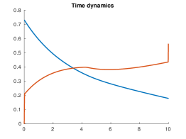
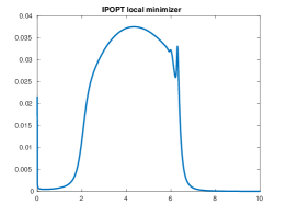
Numerical investigations illustrate this behavior and also hint that the optimal strategies for steering system (1) toward infection establishment may differ significantly from those suitable for (4).


The article is organized as follows. Section 2 is devoted to modeling issues: we introduce the simplified dynamics we consider for the system of wild versus Wolbachia-carrying mosquitoes, as well as the optimal control problem (𝒫fullsubscript𝒫full\mathcal{P}_{\text{full}}) used to design a release strategy.

This problem is then analyzed in Section 3. More precisely, we show in Section 3.1 that (𝒫fullsubscript𝒫full\mathcal{P}_{\text{full}}) and its solution converge to a population replacement strategy optimization problem (𝒫reducedsubscript𝒫reduced\mathcal{P}_{\text{reduced}}) for the simplified model (4), in the limit when birth rates are assumed to be large. Numerical experiments validating our approach are presented in Section 3.2.

2 Toward an optimal control problem

2.1 On the dynamics without control

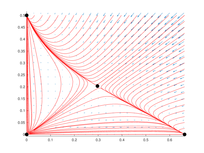
First we describe precisely the asymptotic behavior of System (1) in the absence of control (in other words, when u()=0𝑢0u(\cdot)=0). An example of phase portrait illustrating this lemma is provided on Fig 1. There and for all numerical illustrations of our results, the parameter values we choose for bi,disubscript𝑏𝑖subscript𝑑𝑖b_{i},d_{i} and shsubscript𝑠s_{h} reflect the effects of a Wolbachia infection in Aedes mosquitoes. In the well-documented case of the Wolbachia strain wMel in Aedes aegypti and according to [31, 11], it is relevant to choose: slight fecundity reduction (b2/b10.9similar-to-or-equalssubscript𝑏2subscript𝑏10.9b_{2}/b_{1}\simeq 0.9), slight life-span reduction (d2/d11.1similar-to-or-equalssubscript𝑑2subscript𝑑11.1d_{2}/d_{1}\simeq 1.1) and almost perfect CI (sh=0.9subscript𝑠0.9s_{h}=0.9). We do not fix a time scale, hence the last biologically meaningful parameter is b1/d1subscript𝑏1subscript𝑑1b_{1}/d_{1}, the basic reproduction number for the wild population. Freely inspiried by literature estimates (see [14, 25, 21]) we assume that this number is large, at least equal to 333 (and taking values in all the range [3.7,7400]3.77400[3.7,7400] in Section 3.2). Since these values are used only for results illustration, they are not intended to represent precisely a well-identified mosquito population-Wolbachia strain couple.

Lemma 1.

System (1) is positive and (monotone) competitive777This means that if (n1±,n2±)superscriptsubscript𝑛1plus-or-minussuperscriptsubscript𝑛2plus-or-minus(n_{1}^{\pm},n_{2}^{\pm}) are solutions of (1) such that n1(0)<n1+(0)superscriptsubscript𝑛10superscriptsubscript𝑛10n_{1}^{-}(0)<n_{1}^{+}(0) and n2(0)>n2+(0)superscriptsubscript𝑛20superscriptsubscript𝑛20n_{2}^{-}(0)>n_{2}^{+}(0) then one has n1(t)<n1+(t)superscriptsubscript𝑛1𝑡superscriptsubscript𝑛1𝑡n_{1}^{-}(t)<n_{1}^{+}(t) and n2(t)>n2+(t)superscriptsubscript𝑛2𝑡superscriptsubscript𝑛2𝑡n_{2}^{-}(t)>n_{2}^{+}(t) for every time t[0,T]𝑡0𝑇t\in[0,T], where (n1,n2)superscriptsubscript𝑛1superscriptsubscript𝑛2(n_{1}^{-},n_{2}^{-}) (resp. (n1+,n2+)superscriptsubscript𝑛1superscriptsubscript𝑛2(n_{1}^{+},n_{2}^{+})) denotes the solution of System (1) associated to the choice of initial conditions (n10,n20)=(n1(0),n2(0))superscriptsubscript𝑛10superscriptsubscript𝑛20superscriptsubscript𝑛10superscriptsubscript𝑛20(n_{1}^{0},n_{2}^{0})=(n_{1}^{-}(0),n_{2}^{-}(0)) (resp. (n10,n20)=(n1+(0),n2+(0))superscriptsubscript𝑛10superscriptsubscript𝑛20superscriptsubscript𝑛10superscriptsubscript𝑛20(n_{1}^{0},n_{2}^{0})=(n_{1}^{+}(0),n_{2}^{+}(0))).

Let us assume that

b1>d1 and b2>d2.formulae-sequencesubscript𝑏1subscript𝑑1 and subscript𝑏2subscript𝑑2b_{1}>d_{1}\quad\text{ and }\quad b_{2}>d_{2}. (5)

Then, System (2)-(3) with u()=0𝑢0u(\cdot)=0 has at least three non-negative steady states:

(0,0),(n1,0),(0,n2),withni=K(1dibi),i{1,2}.formulae-sequence00superscriptsubscript𝑛100superscriptsubscript𝑛2withsuperscriptsubscript𝑛𝑖𝐾1subscript𝑑𝑖subscript𝑏𝑖𝑖12(0,0),\quad(n_{1}^{*},0),\quad(0,n_{2}^{*}),\quad\text{with}\quad n_{i}^{*}=K\left(1-\frac{d_{i}}{b_{i}}\right),\ i\in\{1,2\}.

In this case, each population can sustain itself in the absence of the other one. In addition, (0,0)00(0,0) is (locally linearly) unstable.

Moreover, there exists a fourth distinct positive steady state if and only if

1sh<d1b2d2b1<1.1subscript𝑠subscript𝑑1subscript𝑏2subscript𝑑2subscript𝑏111-s_{h}<\frac{d_{1}b_{2}}{d_{2}b_{1}}<1. (6)

In this case, this coexistence equilibrium is (locally linearly) unstable, and is given by

𝐧C=K((11sh(1d1b2d2b1))(1d2b2),1sh(1d1b2d2b1)(1d2b2)).superscript𝐧𝐶𝐾11subscript𝑠1subscript𝑑1subscript𝑏2subscript𝑑2subscript𝑏11subscript𝑑2subscript𝑏21subscript𝑠1subscript𝑑1subscript𝑏2subscript𝑑2subscript𝑏11subscript𝑑2subscript𝑏2\mathbf{n}^{C}=K\left(\left(1-\frac{1}{s_{h}}\left(1-\frac{d_{1}b_{2}}{d_{2}b_{1}}\right)\right)\left(1-\frac{d_{2}}{b_{2}}\right),\frac{1}{s_{h}}\left(1-\frac{d_{1}b_{2}}{d_{2}b_{1}}\right)\left(1-\frac{d_{2}}{b_{2}}\right)\right).

Moreover, the two other nontrivial steady states are locally asymptotically stable in this case.

For the sake of readability, the proof of this result is postponed to Appendix A. Notice that conditions (5) and (6) on the parameters are relevant since Wolbachia-infected Aedes mosquitoes typically have (even slightly) reduced fecundity and lifespan (for instance in the case of wMel strain, [31]). Moreover CI is almost perfect in these species-strain combination (see [11]), i.e. shsubscript𝑠s_{h} is close to 111.

Refer to caption
Figure 1: Phase portrait of System (1) for the parameters choice: b1=0.8subscript𝑏10.8b_{1}=0.8, b2=0.6subscript𝑏20.6b_{2}=0.6, d1=0.27subscript𝑑10.27d_{1}=0.27, d2=0.3subscript𝑑20.3d_{2}=0.3, sh=0.8subscript𝑠0.8s_{h}=0.8 and K=1𝐾1K=1 for which conditions (5) and (6) are satisfied. Examples of trajectories are plotted with continuous lines. The dots locate the four steady states.

Interpretation.

In short, under the biologically relevant conditions (5) and (6), the two mutual exclusion steady states are stable while whole population extinction and coexistence state are unstable: in our model, either one of the two phenotypes must prevail in the long run, eliminating the other one.

2.2 Objective function and constraints on the control

Let us fix a horizon of time T>0𝑇0T>0. In this section, we propose a relevant choice of objective function uJ(u)maps-to𝑢𝐽𝑢u\mapsto J(u), trying to model that we expect the control be chosen so that the final state (at time T𝑇T) of System (1) be as close as possible to the steady state (0,n2)0superscriptsubscript𝑛2(0,n_{2}^{*}) corresponding to a population replacement situation. Since there is no obvious choice, we will consider a least square type functional, having the property to decrease as 𝐧(T)𝐧𝑇\mathbf{n}(T) gets closer to (0,n2)0superscriptsubscript𝑛2(0,n_{2}^{*}).

This leads to introduce

J(u)=12n1(T)2+12[(n2n2(T))+]2,𝐽𝑢12subscript𝑛1superscript𝑇212superscriptdelimited-[]subscriptsuperscriptsubscript𝑛2subscript𝑛2𝑇2J(u)=\frac{1}{2}n_{1}(T)^{2}+\frac{1}{2}\Big{[}(n_{2}^{*}-n_{2}(T))_{+}\Big{]}^{2}, (7)

where, for XIR𝑋IRX\in\mathrm{I\kern-2.10007ptR}, the notation X+subscript𝑋X_{+} stands for max{X,0}𝑋0\max\{X,0\}, and 𝐧=(n1,n2)𝐧subscript𝑛1subscript𝑛2\mathbf{n}=(n_{1},n_{2}) denotes the solution of (1) associated to, in some sense, the worst initial data 𝐧(0)=(n1,0)𝐧0superscriptsubscript𝑛10\mathbf{n}(0)=(n_{1}^{*},0). Notice that, to ensure consistency of our model, any larger value of the introduced population than the equilibrium value n2superscriptsubscript𝑛2n_{2}^{*} is not detrimental for J(u)𝐽𝑢J(u). This objective function differs from the ones introduced in [4, 5], where a L2superscript𝐿2L^{2} norm is used to optimize a similar protocol of Wolbachia infection establishment by releases. Here, we are only interested in the state at the end of the treatment, which determines protocol success or failure.

Let us enumerate the mathematical constraints we will assume on the control function u()𝑢u(\cdot), stemming from biology.

  • u(t)𝑢𝑡u(t) corresponds to the density of Wolbachia-infected released mosquitoes and must be nonnegative (since we assume that we only release individuals and cannot remove them).

  • Since System (1) is monotone, it is relevant to assume an upper bound on the total number of released individuals, namely

    0Tu(t)𝑑tCsuperscriptsubscript0𝑇𝑢𝑡differential-d𝑡𝐶\int_{0}^{T}u(t)dt\leqslant C

    for some given C>0𝐶0C>0. Indeed, releasing more and more individuals can never be detrimental. Without such a constraint, the solution of the considered optimal control problem is trivial and consists in releasing as much individuals as possible at each time.

  • For practical reasons, it is neither possible to create an infinite number of Wolbachia-infected individuals nor to release them “instantly” at time t𝑡t. Hence, this leads to assume a pointwise upper bound on the control, by setting u(t)M𝑢𝑡𝑀u(t)\leqslant M for some M>0𝑀0M>0 and all t[0,T]𝑡0𝑇t\in[0,T]. This constraint models that a release is necessarily distributed in time (possibly on a very short period of time) and cannot be an impulse.

All these considerations lead us to introduce the following set of admissible controls

𝒰T,C,M={uL([0,T]),0uM a.e. ,0Tu(t)dtC}.\boxed{\mathcal{U}_{T,C,M}=\{u\in L^{\infty}([0,T]),\quad 0\leqslant u\leqslant M\text{ a.e. },\int_{0}^{T}u(t)\,dt\leqslant C\}}. (8)

We then deal with the following optimal control problem.

infu𝒰T,C,MJ(u).\boxed{\inf_{u\in\mathcal{U}_{T,C,M}}J(u).} (𝒫fullsubscript𝒫full\mathcal{P}_{\text{full}})

where J𝐽J is defined by (7) and 𝒰T,C,Msubscript𝒰𝑇𝐶𝑀\mathcal{U}_{T,C,M} is defined by (8).

Interpretation.

Problem (𝒫fullsubscript𝒫full\mathcal{P}_{\text{full}}) amounts to finding a constrained release protocol (in terms of total number of released individuals and maximal release flux) which steers the system as close as possible to the target state: elimination of the wild phenotype and establishment of the introduced one.

2.3 System and problem reductions

From a practical point of view, it appears relevant to consider that intrinsic birth rates are large compared with intrinsic death rates, since vector Aedes species typically have a very high reproductive power. For this reason, we will introduce (at the end of this section) and then analyze (in Section 3) a simplified version of Problem (𝒫fullsubscript𝒫full\mathcal{P}_{\text{full}}) that will help to infer some interesting qualitative properties of the solution of Problem (𝒫fullsubscript𝒫full\mathcal{P}_{\text{full}}). This way, we will reduce System (1) into a simple scalar equation on the proportion of Wolbachia-infected mosquitoes in the spirit of [27]. To do so, let us introduce a small parameter ε>0𝜀0\varepsilon>0 and the birth rates

b1=b10/ε and b2=b20/εformulae-sequencesubscript𝑏1superscriptsubscript𝑏10𝜀 and subscript𝑏2superscriptsubscript𝑏20𝜀b_{1}=b_{1}^{0}/\varepsilon\quad\text{ and }\quad b_{2}=b_{2}^{0}/\varepsilon (9)

for some positive numbers b10superscriptsubscript𝑏10b_{1}^{0}, b20superscriptsubscript𝑏20b_{2}^{0}.

It is notable that, in that case, the steady-states (n1,0)superscriptsubscript𝑛10(n_{1}^{*},0) and (0,n2)0superscriptsubscript𝑛2(0,n_{2}^{*}) respectively converge to (K,0)𝐾0(K,0) and (0,K)0𝐾(0,K) as ε0𝜀0\varepsilon\searrow 0, since ni=K(1εdibi0)superscriptsubscript𝑛𝑖𝐾1𝜀subscript𝑑𝑖superscriptsubscript𝑏𝑖0n_{i}^{*}=K(1-\varepsilon\frac{d_{i}}{b_{i}^{0}}), i=1,2𝑖12i=1,2. Notice also that (5) is automatically satisfied as soon as ε𝜀\varepsilon is small enough.

In what follows, we will denote by Jεsuperscript𝐽𝜀J^{\varepsilon} the functional defined by

Jε(u)=12n1ε(T)2+12(n2n2ε(T))+2,superscript𝐽𝜀𝑢12superscriptsubscript𝑛1𝜀superscript𝑇212superscriptsubscriptsuperscriptsubscript𝑛2superscriptsubscript𝑛2𝜀𝑇2J^{\varepsilon}(u)=\frac{1}{2}n_{1}^{\varepsilon}(T)^{2}+\frac{1}{2}(n_{2}^{*}-n_{2}^{\varepsilon}(T))_{+}^{2}, (10)

where (n1ε,n2ε)superscriptsubscript𝑛1𝜀superscriptsubscript𝑛2𝜀(n_{1}^{\varepsilon},n_{2}^{\varepsilon}) denote the solution to Problem (1) with b1subscript𝑏1b_{1} and b2subscript𝑏2b_{2} given by (9). Let us introduce the variables

Nε=n1ε+n2ε and pε=n2ε/Nε.formulae-sequencesuperscript𝑁𝜀superscriptsubscript𝑛1𝜀superscriptsubscript𝑛2𝜀 and superscript𝑝𝜀superscriptsubscript𝑛2𝜀superscript𝑁𝜀N^{\varepsilon}=n_{1}^{\varepsilon}+n_{2}^{\varepsilon}\qquad\text{ and }\qquad p^{\varepsilon}=n_{2}^{\varepsilon}/N^{\varepsilon}. (11)

Setting nε=1ε(1NεK)superscript𝑛𝜀1𝜀1superscript𝑁𝜀𝐾n^{\varepsilon}=\frac{1}{\varepsilon}\left(1-\frac{N^{\varepsilon}}{K}\right), we have the following (technical but crucial) convergence result, saying that the pair (nε,pε)superscript𝑛𝜀superscript𝑝𝜀(n^{\varepsilon},p^{\varepsilon}) converges in some sense to a well-identified limit (u,p)𝑢𝑝(u,p).

Proposition 1.

Let uε𝒰T,C,Msuperscript𝑢𝜀subscript𝒰𝑇𝐶𝑀u^{\varepsilon}\in\mathcal{U}_{T,C,M} such that (uε)ε>0subscriptsuperscript𝑢𝜀𝜀0(u^{\varepsilon})_{\varepsilon>0} converges weakly-star to u𝒰T,C,M𝑢subscript𝒰𝑇𝐶𝑀u\in\mathcal{U}_{T,C,M} in L(0,T)superscript𝐿0𝑇L^{\infty}(0,T) as ε0𝜀0\varepsilon\searrow 0.

The pair (nε,pε)superscript𝑛𝜀superscript𝑝𝜀(n^{\varepsilon},p^{\varepsilon}) associated to the control uεsuperscript𝑢𝜀u^{\varepsilon} and the parameter scaling (9) solves a slow-fast system of the form

{εdnεdt=(1εnε)a(pε)(Z(pε)nε)uεK,dpεdt=pε(1pε)(nε(b20b10(1shpε))+d1d2)+uε(1pε)K(1εnε),t>0nε(0)=d10b10,pε(0)=0,cases𝜀𝑑superscript𝑛𝜀𝑑𝑡1𝜀superscript𝑛𝜀𝑎superscript𝑝𝜀𝑍superscript𝑝𝜀superscript𝑛𝜀superscript𝑢𝜀𝐾formulae-sequence𝑑superscript𝑝𝜀𝑑𝑡superscript𝑝𝜀1superscript𝑝𝜀superscript𝑛𝜀superscriptsubscript𝑏20superscriptsubscript𝑏101subscript𝑠superscript𝑝𝜀subscript𝑑1subscript𝑑2superscript𝑢𝜀1superscript𝑝𝜀𝐾1𝜀superscript𝑛𝜀𝑡0formulae-sequencesuperscript𝑛𝜀0superscriptsubscript𝑑10superscriptsubscript𝑏10superscript𝑝𝜀00\left\{\begin{array}[]{l}\varepsilon\displaystyle\frac{dn^{\varepsilon}}{dt}=(1-\varepsilon n^{\varepsilon})a(p^{\varepsilon})\big{(}Z(p^{\varepsilon})-n^{\varepsilon}\big{)}-\frac{u^{\varepsilon}}{K},\\[10.0pt] \displaystyle\frac{dp^{\varepsilon}}{dt}=p^{\varepsilon}(1-p^{\varepsilon})\big{(}n^{\varepsilon}(b_{2}^{0}-b_{1}^{0}(1-s_{h}p^{\varepsilon}))+d_{1}-d_{2}\big{)}+\frac{u^{\varepsilon}(1-p^{\varepsilon})}{K(1-\varepsilon n^{\varepsilon})},\quad t>0\\[10.0pt] \displaystyle n^{\varepsilon}(0)=\frac{d_{1}^{0}}{b_{1}^{0}},\ p^{\varepsilon}(0)=0,\end{array}\right. (12)

where a(p)𝑎𝑝a(p) and Z(p)𝑍𝑝Z(p) are defined by

a(p)=b10(1p)(1shp)+b20p>0,Z(p)=d1(1p)+d2pa(p)>0.formulae-sequence𝑎𝑝superscriptsubscript𝑏101𝑝1subscript𝑠𝑝superscriptsubscript𝑏20𝑝0𝑍𝑝subscript𝑑11𝑝subscript𝑑2𝑝𝑎𝑝0a(p)=b_{1}^{0}(1-p)(1-s_{h}p)+b_{2}^{0}p>0,\quad Z(p)=\frac{d_{1}(1-p)+d_{2}p}{a(p)}>0.

Let us assume that (6) holds and let ε0>0subscript𝜀00\varepsilon_{0}>0 be such that

d1b10<1ε0 and max[0,1]Z<1ε0.formulae-sequencesubscript𝑑1superscriptsubscript𝑏101subscript𝜀0 and subscript01𝑍1subscript𝜀0\frac{d_{1}}{b_{1}^{0}}<\frac{1}{\varepsilon_{0}}\quad\text{ and }\quad\max_{[0,1]}Z<\frac{1}{\varepsilon_{0}}. (13)

Then, for all ε(0,ε0)𝜀0subscript𝜀0\varepsilon\in(0,\varepsilon_{0}), we have the uniform estimates

0pε(t)1 and nnε(t)n+formulae-sequence0superscript𝑝𝜀𝑡1 and subscript𝑛superscript𝑛𝜀𝑡subscript𝑛0\leqslant p^{\varepsilon}(t)\leqslant 1\quad\text{ and }\quad n_{-}\leqslant n^{\varepsilon}(t)\leqslant n_{+} (14)

for all t[0,T]𝑡0𝑇t\in[0,T] where

nsubscript𝑛\displaystyle n_{-} =\displaystyle= min{d1b10,minε[0,ε0]minp[0,1]1+εZ(p)(1εZ(p))2+4εM/(Ka(p))2ε}subscript𝑑1superscriptsubscript𝑏10subscript𝜀0subscript𝜀0subscript𝑝011𝜀𝑍𝑝superscript1𝜀𝑍𝑝24𝜀𝑀𝐾𝑎𝑝2𝜀\displaystyle\min\left\{\frac{d_{1}}{b_{1}^{0}},\min_{\varepsilon\in[0,\varepsilon_{0}]}\min_{p\in[0,1]}\frac{1+\varepsilon Z(p)-\sqrt{(1-\varepsilon Z(p))^{2}+4\varepsilon M/(Ka(p))}}{2\varepsilon}\right\}
n+subscript𝑛\displaystyle n_{+} =\displaystyle= max{d1b10,maxp[0,1]Z(p)}.subscript𝑑1superscriptsubscript𝑏10subscript𝑝01𝑍𝑝\displaystyle\max\left\{\frac{d_{1}}{b_{1}^{0}},\max_{p\in[0,1]}Z(p)\right\}.

Moreover, up to a subfamily, (pε)ε>0subscriptsuperscript𝑝𝜀𝜀0(p^{\varepsilon})_{\varepsilon>0} converges uniformly as ε0𝜀0\varepsilon\searrow 0 to p𝑝p, solving

{dpdt=f(p)+ug(p),t>0p(0)=0casesformulae-sequence𝑑𝑝𝑑𝑡𝑓𝑝𝑢𝑔𝑝𝑡0𝑝00\left\{\begin{array}[]{l}\displaystyle\frac{dp}{dt}=f(p)+ug(p),\quad t>0\\[10.0pt] p(0)=0\end{array}\right. (15)

where

f(p)=p(1p)d1b20d2b10(1shp)b10(1p)(1shp)+b20pandg(p)=1Kb10(1p)(1shp)b10(1p)(1shp)+b20p.formulae-sequence𝑓𝑝𝑝1𝑝subscript𝑑1superscriptsubscript𝑏20subscript𝑑2superscriptsubscript𝑏101subscript𝑠𝑝superscriptsubscript𝑏101𝑝1subscript𝑠𝑝superscriptsubscript𝑏20𝑝and𝑔𝑝1𝐾superscriptsubscript𝑏101𝑝1subscript𝑠𝑝superscriptsubscript𝑏101𝑝1subscript𝑠𝑝superscriptsubscript𝑏20𝑝f(p)=p(1-p)\frac{d_{1}b_{2}^{0}-d_{2}b_{1}^{0}(1-s_{h}p)}{b_{1}^{0}(1-p)(1-s_{h}p)+b_{2}^{0}p}\quad\text{and}\quad g(p)=\frac{1}{K}\cdot\frac{b_{1}^{0}(1-p)(1-s_{h}p)}{b_{1}^{0}(1-p)(1-s_{h}p)+b_{2}^{0}p}. (16)

Interpretation.

Proposition 16 is a rigorous result showing that a single equation on the proportion of Wolbachia-carrying mosquitoes (equation (15)) is a fair approximation of the time dynamics induced by the model with two populations (1), provided that the fecundity is large.

Remark 1.

It is notable that the function [0,ε0]ε1+εZ(p)(1εZ(p))2+4εM/(Ka(p))2εcontains0subscript𝜀0𝜀maps-to1𝜀𝑍𝑝superscript1𝜀𝑍𝑝24𝜀𝑀𝐾𝑎𝑝2𝜀[0,\varepsilon_{0}]\ni\varepsilon\mapsto\frac{1+\varepsilon Z(p)-\sqrt{(1-\varepsilon Z(p))^{2}+4\varepsilon M/(Ka(p))}}{2\varepsilon} used to define nsubscript𝑛n_{-} in the statement of Proposition 16 above converges to the finite (and bounded in p[0,1]𝑝01p\in[0,1]) value Z(p)M/(Ka(p))𝑍𝑝𝑀𝐾𝑎𝑝Z(p)-M/(Ka(p)) as ε0𝜀0\varepsilon\to 0. Therefore nsubscript𝑛n_{-} is uniformly bounded for ε[0,ε0]𝜀0subscript𝜀0\varepsilon\in[0,\varepsilon_{0}].

Refer to caption
Figure 2: Equation (15) is the form dpdt=f(p)+ug(p),𝑑𝑝𝑑𝑡𝑓𝑝𝑢𝑔𝑝\frac{dp}{dt}=f(p)+ug(p), with f𝑓f of bistable type (see Footnote 6). Plot of the right-hand side function f𝑓f with the same parameters values as in Figure 1.
Proof.

System (1) reads

{dn1εdt=b10n1ε(1shpε)nεd1n1εdn2εdt=b20n2εnεd2n2ε+uε.cases𝑑superscriptsubscript𝑛1𝜀𝑑𝑡absentsuperscriptsubscript𝑏10superscriptsubscript𝑛1𝜀1subscript𝑠superscript𝑝𝜀superscript𝑛𝜀subscript𝑑1superscriptsubscript𝑛1𝜀𝑑superscriptsubscript𝑛2𝜀𝑑𝑡absentsuperscriptsubscript𝑏20superscriptsubscript𝑛2𝜀superscript𝑛𝜀subscript𝑑2superscriptsubscript𝑛2𝜀superscript𝑢𝜀\begin{cases}\displaystyle\frac{dn_{1}^{\varepsilon}}{dt}=&b_{1}^{0}n_{1}^{\varepsilon}(1-s_{h}p^{\varepsilon})n^{\varepsilon}-d_{1}n_{1}^{\varepsilon}\\[10.0pt] \displaystyle\frac{dn_{2}^{\varepsilon}}{dt}=&b_{2}^{0}n_{2}^{\varepsilon}n^{\varepsilon}-d_{2}n_{2}^{\varepsilon}+u^{\varepsilon}.\end{cases} (17)

Hence, the resulting system (12) on (nε,pε)superscript𝑛𝜀superscript𝑝𝜀(n^{\varepsilon},p^{\varepsilon}) in Proposition 16 is obtained from straightforward computations.

Let us now provide a priori bounds on (nε(t),pε(t))superscript𝑛𝜀𝑡superscript𝑝𝜀𝑡(n^{\varepsilon}(t),p^{\varepsilon}(t)) (uniform in εε0𝜀subscript𝜀0\varepsilon\leqslant\varepsilon_{0}, for all t0𝑡0t\geqslant 0). Note that 0pε10superscript𝑝𝜀10\leqslant p^{\varepsilon}\leqslant 1 is an easy consequence of the Cauchy-Lipschitz theorem since pε=0superscript𝑝𝜀0p^{\varepsilon}=0 and pε=1superscript𝑝𝜀1p^{\varepsilon}=1 are respectively sub- and super-solutions.

We infer that the right-hand side of the equation on nεsuperscript𝑛𝜀n^{\varepsilon} in (12) is bounded from below by

a(p)(1εn)(Z(p)n)MK,𝑎𝑝1𝜀𝑛𝑍𝑝𝑛𝑀𝐾a(p)(1-\varepsilon n)(Z(p)-n)-\frac{M}{K},

which is positive as soon as n𝑛n is smaller than the smallest root of this second order polynomial in n𝑛n given by

a(p)(1+εZ(p))a(p)(1εZ(p))2+4εM/(Ka(p))2a(p)ε.𝑎𝑝1𝜀𝑍𝑝𝑎𝑝superscript1𝜀𝑍𝑝24𝜀𝑀𝐾𝑎𝑝2𝑎𝑝𝜀\frac{a(p)(1+\varepsilon Z(p))-a(p)\sqrt{(1-\varepsilon Z(p))^{2}+4\varepsilon M/(Ka(p))}}{2a(p)\varepsilon}.

Moreover, the right-hand side of the equation on nεsuperscript𝑛𝜀n^{\varepsilon} in (12) is bounded from above by

a(p)(1εn)(Z(p)n),𝑎𝑝1𝜀𝑛𝑍𝑝𝑛a(p)(1-\varepsilon n)(Z(p)-n),

which is negative as soon as n𝑛n is between Z(p)𝑍𝑝Z(p) and 1/ε1𝜀1/\varepsilon. We then infer the expected uniform estimates on nεsuperscript𝑛𝜀n^{\varepsilon} as soon as ε0subscript𝜀0\varepsilon_{0} is small enough.

We are then driven to the slow-fast system (12). Using the uniform bounds on nεsuperscript𝑛𝜀n^{\varepsilon}, pεsuperscript𝑝𝜀p^{\varepsilon}, uεsuperscript𝑢𝜀u^{\varepsilon}, we infer that the right-hand sides are bounded. Hence, by using the Arzelà-Ascoli theorem, we get that (pε)ε>0subscriptsuperscript𝑝𝜀𝜀0(p^{\varepsilon})_{\varepsilon>0} converges up to a subfamily uniformly to some function p𝑝p such that p(0)=0𝑝00p(0)=0 and 0p10𝑝10\leqslant p\leqslant 1 as ε0𝜀0\varepsilon\searrow 0. Moreover, dp/dt𝑑𝑝𝑑𝑡dp/dt is uniformly bounded since dpε/dt𝑑superscript𝑝𝜀𝑑𝑡dp^{\varepsilon}/dt is.

According to Lemma 3 below, the limit p𝑝p satisfies

dpdt=f(p)+ug(p),p(0)=0,formulae-sequence𝑑𝑝𝑑𝑡𝑓𝑝𝑢𝑔𝑝𝑝00\frac{dp}{dt}=f(p)+ug(p),\quad p(0)=0,

with f𝑓f and g𝑔g defined by (16). Since the solution to this equation is unique, we finally get the uniform convergence of the whole family (pε)ε>0subscriptsuperscript𝑝𝜀𝜀0(p^{\varepsilon})_{\varepsilon>0} to p𝑝p. ∎

The two following technical lemmata are used in the proof of Proposition 16.

Lemma 2.

Up to a subfamily, the family (nε)ε>0subscriptsuperscript𝑛𝜀𝜀0(n^{\varepsilon})_{\varepsilon>0} converges weakly to Z(p)ua(p)K𝑍𝑝𝑢𝑎𝑝𝐾Z(p)-\frac{u}{a(p)K} as ε0𝜀0\varepsilon\searrow 0 in (W1,1)superscriptsuperscript𝑊11(W^{1,1})^{\prime}, with p𝑝p the uniform limit of any subfamily (pε)ε>0subscriptsuperscript𝑝𝜀𝜀0(p^{\varepsilon})_{\varepsilon>0}.

Proof.

Let ϕW1,1italic-ϕsuperscript𝑊11\phi\in W^{1,1} and multiply the differential equation satisfied by nεsuperscript𝑛𝜀n^{\varepsilon} by ϕitalic-ϕ\phi and integrate by parts over [0,T]0𝑇[0,T]. We get

ε[ϕnε]0Tε0Tdϕdtnε=0Tϕa(pε)(Z(pε)nε)0TϕuεK.𝜀superscriptsubscriptdelimited-[]italic-ϕsuperscript𝑛𝜀0𝑇𝜀superscriptsubscript0𝑇𝑑italic-ϕ𝑑𝑡superscript𝑛𝜀superscriptsubscript0𝑇italic-ϕ𝑎superscript𝑝𝜀𝑍superscript𝑝𝜀superscript𝑛𝜀superscriptsubscript0𝑇italic-ϕsuperscript𝑢𝜀𝐾\varepsilon[\phi n^{\varepsilon}]_{0}^{T}-\varepsilon\int_{0}^{T}\frac{d\phi}{dt}n^{\varepsilon}=\int_{0}^{T}\phi a(p^{\varepsilon})(Z(p^{\varepsilon})-n^{\varepsilon})-\int_{0}^{T}\phi\frac{u^{\varepsilon}}{K}.

By weak-star convergence of uεsuperscript𝑢𝜀u^{\varepsilon} in Lsuperscript𝐿L^{\infty}, uniform convergence of pεsuperscript𝑝𝜀p^{\varepsilon} in Lsuperscript𝐿L^{\infty} and uniform boundedness of nεsuperscript𝑛𝜀n^{\varepsilon} we infer that

0=limε00Tϕa(pε)(Z(pε)nε)0TϕuK,0subscript𝜀0superscriptsubscript0𝑇italic-ϕ𝑎superscript𝑝𝜀𝑍superscript𝑝𝜀superscript𝑛𝜀superscriptsubscript0𝑇italic-ϕ𝑢𝐾0=\lim_{\varepsilon\to 0}\int_{0}^{T}\phi a(p^{\varepsilon})(Z(p^{\varepsilon})-n^{\varepsilon})-\int_{0}^{T}\phi\frac{u}{K},

leading to the expected result. ∎

Lemma 3.

Up to a subfamily, (pε)ε>0subscriptsuperscript𝑝𝜀𝜀0(p^{\varepsilon})_{\varepsilon>0} converges uniformly to p𝑝p solving the ordinary differential equation

dpdt=f(p)+ug(p),p(0)=0,formulae-sequence𝑑𝑝𝑑𝑡𝑓𝑝𝑢𝑔𝑝𝑝00\frac{dp}{dt}=f(p)+ug(p),\quad p(0)=0,

with f𝑓f and g𝑔g defined by (16).

Proof.

Let us first recast the equation on pεsuperscript𝑝𝜀p^{\varepsilon} in system (12) under the form

dpεdt=βε(nε,pε,uε),pε(0)=0,formulae-sequence𝑑superscript𝑝𝜀𝑑𝑡subscript𝛽𝜀superscript𝑛𝜀superscript𝑝𝜀superscript𝑢𝜀superscript𝑝𝜀00\frac{dp^{\varepsilon}}{dt}=\beta_{\varepsilon}(n^{\varepsilon},p^{\varepsilon},u^{\varepsilon}),\quad p^{\varepsilon}(0)=0,

with

βε(n,p,u)=p(1p)(n(b20b10(1shp))+d1d2)+u(1p)K(1εn)subscript𝛽𝜀𝑛𝑝𝑢𝑝1𝑝𝑛superscriptsubscript𝑏20superscriptsubscript𝑏101subscript𝑠𝑝subscript𝑑1subscript𝑑2𝑢1𝑝𝐾1𝜀𝑛\beta_{\varepsilon}(n,p,u)=p(1-p)\big{(}n(b_{2}^{0}-b_{1}^{0}(1-s_{h}p))+d_{1}-d_{2}\big{)}+\frac{u(1-p)}{K(1-\varepsilon n)}

so that we easily infer (with obvious notations) that βεβsubscript𝛽𝜀𝛽\beta_{\varepsilon}\to\beta as ε0𝜀0\varepsilon\searrow 0 with βε(n,p,u)=nβ^(p)+β0(p)+uβ~ε(n,p)subscript𝛽𝜀𝑛𝑝𝑢𝑛^𝛽𝑝subscript𝛽0𝑝𝑢superscript~𝛽𝜀𝑛𝑝\beta_{\varepsilon}(n,p,u)=n\widehat{\beta}(p)+\beta_{0}(p)+u\widetilde{\beta}^{\varepsilon}(n,p), β(n,p,u)=nβ^(p)+β0(p)+uβ~(p)𝛽𝑛𝑝𝑢𝑛^𝛽𝑝subscript𝛽0𝑝𝑢~𝛽𝑝\beta(n,p,u)=n\widehat{\beta}(p)+\beta_{0}(p)+u\widetilde{\beta}(p), β^(p)=p(1p)(b20b10(1shp))^𝛽𝑝𝑝1𝑝superscriptsubscript𝑏20superscriptsubscript𝑏101subscript𝑠𝑝\widehat{\beta}(p)=p(1-p)(b_{2}^{0}-b_{1}^{0}(1-s_{h}p)), β0(p)=(d1d2)p(1p)subscript𝛽0𝑝subscript𝑑1subscript𝑑2𝑝1𝑝\beta_{0}(p)=(d_{1}-d_{2})p(1-p) and β~(p)=1pK(1εn)~𝛽𝑝1𝑝𝐾1𝜀𝑛\widetilde{\beta}(p)=\frac{1-p}{K(1-\varepsilon n)}.

Using the previous considerations (and in particular the uniform boundedness of pεsuperscript𝑝𝜀p^{\varepsilon}, nεsuperscript𝑛𝜀n^{\varepsilon} and uεsuperscript𝑢𝜀u^{\varepsilon}), we deduce that p𝑝p is in fact Lipschitz-continuous, and that β^^𝛽\widehat{\beta} and β~~𝛽\widetilde{\beta} are continuous on [0,1]01[0,1].

Now, let us show that p𝑝p satisfies the limit equation in a weak sense. Let ϕ𝒞c(0,T)italic-ϕsuperscriptsubscript𝒞𝑐0𝑇\phi\in\mathcal{C}_{c}^{\infty}(0,T). We compute each term separately: the terms in dpε/dt𝑑superscript𝑝𝜀𝑑𝑡dp^{\varepsilon}/dt and β0(pε)subscript𝛽0superscript𝑝𝜀\beta_{0}(p^{\varepsilon}) converge by uniform convergence of pεsuperscript𝑝𝜀p^{\varepsilon}. Therefore, we have

0Tϕnεβ^(pε)=0Tϕnεβ^(p)0Tϕnβ^(p)+0Tϕnε(β^(pε)β^(p))||nεo(1).superscriptsubscript0𝑇italic-ϕsuperscript𝑛𝜀^𝛽superscript𝑝𝜀subscriptsuperscriptsubscript0𝑇italic-ϕsuperscript𝑛𝜀^𝛽𝑝absentsuperscriptsubscript0𝑇italic-ϕ𝑛^𝛽𝑝subscriptsuperscriptsubscript0𝑇italic-ϕsuperscript𝑛𝜀^𝛽superscript𝑝𝜀^𝛽𝑝subscriptdelimited-∥∥superscript𝑛𝜀𝑜1\int_{0}^{T}\phi n^{\varepsilon}\widehat{\beta}(p^{\varepsilon})=\underbrace{\int_{0}^{T}\phi n^{\varepsilon}\widehat{\beta}(p)}_{\to\int_{0}^{T}\phi n\widehat{\beta}(p)}+\underbrace{\int_{0}^{T}\phi n^{\varepsilon}\big{(}\widehat{\beta}(p^{\varepsilon})-\widehat{\beta}(p)\big{)}}_{\lvert\cdot\rvert\leqslant\lVert n^{\varepsilon}\rVert_{\infty}o(1)}.

and

0Tϕuεβ~ε(nε,pε)=0Tϕuεβ~(p)0Tϕuβ~(p)+0Tϕuε(β~ε(nε,pε)β~(p))||Mo(1).superscriptsubscript0𝑇italic-ϕsuperscript𝑢𝜀superscript~𝛽𝜀superscript𝑛𝜀superscript𝑝𝜀subscriptsuperscriptsubscript0𝑇italic-ϕsuperscript𝑢𝜀~𝛽𝑝absentsuperscriptsubscript0𝑇italic-ϕ𝑢~𝛽𝑝subscriptsuperscriptsubscript0𝑇italic-ϕsuperscript𝑢𝜀superscript~𝛽𝜀superscript𝑛𝜀superscript𝑝𝜀~𝛽𝑝𝑀𝑜1\int_{0}^{T}\phi u^{\varepsilon}\widetilde{\beta}^{\varepsilon}(n^{\varepsilon},p^{\varepsilon})=\underbrace{\int_{0}^{T}\phi u^{\varepsilon}\widetilde{\beta}(p)}_{\to\int_{0}^{T}\phi u\widetilde{\beta}(p)}+\underbrace{\int_{0}^{T}\phi u^{\varepsilon}\big{(}\widetilde{\beta}^{\varepsilon}(n^{\varepsilon},p^{\varepsilon})-\widetilde{\beta}(p)\big{)}}_{\lvert\cdot\rvert\leqslant Mo(1)}.

by using simultaneously the weak convergence properties of (uε)ε>0subscriptsuperscript𝑢𝜀𝜀0(u^{\varepsilon})_{\varepsilon>0} and (nε)ε>0subscriptsuperscript𝑛𝜀𝜀0(n^{\varepsilon})_{\varepsilon>0} (see Lemma 2) as well as the aforementioned convergence of βεsubscript𝛽𝜀\beta_{\varepsilon} to β𝛽\beta. Here, it is crucial that the limit β~~𝛽\widetilde{\beta} does not depend on n𝑛n but merely on p𝑝p, and we rely on the uniform estimate on nεsuperscript𝑛𝜀n^{\varepsilon}.

Finally, a standard argument yields that p𝑝p must satisfy the equation in a strong sense since it is Lipschitz-continuous. ∎

We are now in position to determine the asymptotic behavior of the solutions of Problem (𝒫fullsubscript𝒫full\mathcal{P}_{\text{full}}) as ε0𝜀0\varepsilon\searrow 0, in the case where (9) is assumed.

We have already observed that the invasion equilibrium (0,n2)0superscriptsubscript𝑛2(0,n_{2}^{*}) is in particular changed into (0,K(1εd2b20))0𝐾1𝜀subscript𝑑2superscriptsubscript𝑏20(0,K(1-\varepsilon\frac{d_{2}}{b_{2}^{0}})), which converges to (0,K)0𝐾(0,K) as ε0𝜀0\varepsilon\searrow 0. By using the result stated in Proposition 16, we formally infer that (Nε(T))ε>0subscriptsuperscript𝑁𝜀𝑇𝜀0(N^{\varepsilon}(T))_{\varepsilon>0} converges to K𝐾K and (pε(T))ε>0subscriptsuperscript𝑝𝜀𝑇𝜀0(p^{\varepsilon}(T))_{\varepsilon>0} converges to some limit p(T)[0,1]𝑝𝑇01p(T)\in[0,1] as ε0𝜀0\varepsilon\searrow 0, meaning that (n1ε(T),n2ε(T)))ε>0(n_{1}^{\varepsilon}(T),n_{2}^{\varepsilon}(T)))_{\varepsilon>0} converges to (K(1p(T)),Kp(T))𝐾1𝑝𝑇𝐾𝑝𝑇(K(1-p(T)),Kp(T)). It follows that Jε(u)superscript𝐽𝜀𝑢J^{\varepsilon}(u) converges, as ε0𝜀0\varepsilon\searrow 0 to

K22(1p(T))2+K22(1p(T))2=K2(1p(T))2,superscript𝐾22superscript1𝑝𝑇2superscript𝐾22superscript1𝑝𝑇2superscript𝐾2superscript1𝑝𝑇2\frac{K^{2}}{2}(1-p(T))^{2}+\frac{K^{2}}{2}(1-p(T))^{2}=K^{2}(1-p(T))^{2},

where p𝑝p denotes the solution of (15).

This leads to introduce an asymptotic version J0superscript𝐽0J^{0} of the cost function Jεsuperscript𝐽𝜀J^{\varepsilon} given by

J0(u)=K2(1p(T))2,superscript𝐽0𝑢superscript𝐾2superscript1𝑝𝑇2J^{0}(u)=K^{2}(1-p(T))^{2}, (18)

as well as an asymptotic version of Problem (𝒫fullsubscript𝒫full\mathcal{P}_{\text{full}}) reading

infu𝒰T,C,M(1p(T))2,\boxed{\inf_{u\in\mathcal{U}_{T,C,M}}(1-p(T))^{2},} (𝒫reducedsubscript𝒫reduced\mathcal{P}_{\text{reduced}})

where p𝑝p solves (15) and 𝒰T,C,Msubscript𝒰𝑇𝐶𝑀\mathcal{U}_{T,C,M} is defined by (8).

In Section 3, we will analyze the connections between Problem (𝒫fullsubscript𝒫full\mathcal{P}_{\text{full}}) and Problem (𝒫reducedsubscript𝒫reduced\mathcal{P}_{\text{reduced}}), by providing a description of minimizers and highlighting good convergence properties as ε0𝜀0\varepsilon\searrow 0.

3 Analysis of Problem (𝒫fullsubscript𝒫full\mathcal{P}_{\text{full}}) and numerics

3.1 Description of minimizers

This section is devoted to the analysis of Problems (𝒫fullsubscript𝒫full\mathcal{P}_{\text{full}}) and (𝒫reducedsubscript𝒫reduced\mathcal{P}_{\text{reduced}}). It mainly contains two results:

Definition 1 (ΓΓ\Gamma-convergence, [3]).

One says that Jεsuperscript𝐽𝜀J^{\varepsilon} ΓΓ\Gamma-converges to J0superscript𝐽0J^{0} if for u𝒰T,C,M𝑢subscript𝒰𝑇𝐶𝑀u\in\mathcal{U}_{T,C,M} and (uε)ε>0subscriptsuperscript𝑢𝜀𝜀0(u^{\varepsilon})_{\varepsilon>0} converging weak-star to u𝑢u in L(0,T)superscript𝐿0𝑇L^{\infty}(0,T), one has

lim infε0Jε(uε)J0(u)subscriptlimit-infimum𝜀0superscript𝐽𝜀superscript𝑢𝜀superscript𝐽0𝑢\liminf_{\varepsilon\to 0}J^{\varepsilon}(u^{\varepsilon})\geqslant J^{0}(u) (19)

and there exists a sequence (u¯ε)εsubscriptsuperscript¯𝑢𝜀𝜀(\overline{u}^{\varepsilon})_{\varepsilon}, with u¯εusuperscript¯𝑢𝜀𝑢\overline{u}^{\varepsilon}\rightharpoonup u, such that

lim supε0Jε(u¯ε)J0(u).subscriptlimit-supremum𝜀0superscript𝐽𝜀superscript¯𝑢𝜀superscript𝐽0𝑢\limsup_{\varepsilon\to 0}J^{\varepsilon}(\overline{u}^{\varepsilon})\leqslant J^{0}(u). (20)

To investigate the convergence of minimizers for Problem (𝒫fullsubscript𝒫full\mathcal{P}_{\text{full}}), we will use the fundamental theorem of ΓΓ\Gamma-convergence (see e.g. [3, Theorem 2.10]) stating that, under a ΓΓ\Gamma-convergence property and equicoercivity of the considered functional, closure points of the sequence of minimizers are themselves solution of an asymptotic problem.

Proposition 2.

Let T,C,M>0𝑇𝐶𝑀0T,C,M>0 and assume that (5) and (6) hold. Problem (𝒫fullsubscript𝒫full\mathcal{P}_{\text{full}}) and Problem (𝒫reducedsubscript𝒫reduced\mathcal{P}_{\text{reduced}}) have (at least) a solution.

Moreover, let (uε)ε>0subscriptsuperscript𝑢𝜀𝜀0(u^{\varepsilon})_{\varepsilon>0} be a family of minimizers for Problem (𝒫fullsubscript𝒫full\mathcal{P}_{\text{full}}). Then, one has

limε0infu𝒰T,C,MJε(u)=infu𝒰T,C,MJ0(u)subscript𝜀0subscriptinfimum𝑢subscript𝒰𝑇𝐶𝑀superscript𝐽𝜀𝑢subscriptinfimum𝑢subscript𝒰𝑇𝐶𝑀superscript𝐽0𝑢\lim_{\varepsilon\searrow 0}\inf_{u\in\mathcal{U}_{T,C,M}}J^{\varepsilon}(u)=\inf_{u\in\mathcal{U}_{T,C,M}}J^{0}(u)

and any closure point of this family (as ε0𝜀0\varepsilon\searrow 0, for the Lsuperscript𝐿L^{\infty}-weak star topology) is a solution of Problem (𝒫reducedsubscript𝒫reduced\mathcal{P}_{\text{reduced}}).

Interpretation.

Proposition 2 establishes that the controlled scalar equation (15) is not only a fair approximation of the time dynamics of the infection frequency n2/(n1+n2)subscript𝑛2subscript𝑛1subscript𝑛2n_{2}/(n_{1}+n_{2}) from system (1), but also provides a sound framework for studying optimization problems. Morally, a release protocol defined by solving the simpler problem (𝒫reducedsubscript𝒫reduced\mathcal{P}_{\text{reduced}}) will be typically good for (𝒫fullsubscript𝒫full\mathcal{P}_{\text{full}}) as well, provided that the fecundity is large.

We now solve Problem (𝒫reducedsubscript𝒫reduced\mathcal{P}_{\text{reduced}}) involving p𝑝p, the solution to (4). In other words

dpdt=f(p)+ug(p),𝑑𝑝𝑑𝑡𝑓𝑝𝑢𝑔𝑝\frac{dp}{dt}=f(p)+ug(p),

Moreover, in what follows, we assume that (6) is satisfied and will mainly use structural properties of f𝑓f and g𝑔g. Namely they are C1superscript𝐶1C^{1} functions on [0,1]01[0,1] such that g>0𝑔0g>0 on [0,1)01[0,1), g(1)=0𝑔10g(1)=0, and f𝑓f is a bistable function (see Footnote 6). We denote by θ𝜃\theta the unique real number satisfying

f(θ)=0andθ(0,1),formulae-sequence𝑓𝜃0and𝜃01f(\theta)=0\qquad\text{and}\qquad\theta\in(0,1),

where f𝑓f is given by (16), in other words,

θ=1sh(1d1b20d2b10).𝜃1subscript𝑠1subscript𝑑1superscriptsubscript𝑏20subscript𝑑2superscriptsubscript𝑏10\theta=\frac{1}{s_{h}}\left(1-\frac{d_{1}b_{2}^{0}}{d_{2}b_{1}^{0}}\right). (21)
Proof.

Let us first investigate the existence of solutions for Problem (𝒫fullsubscript𝒫full\mathcal{P}_{\text{full}}) under the assumption (9).

Fix ε>0𝜀0\varepsilon>0 and consider (unε)nINsubscriptsuperscriptsubscript𝑢𝑛𝜀𝑛IN(u_{n}^{\varepsilon})_{n\in\mathrm{I\kern-1.47005ptN}} a minimizing sequence. According to the Banach-Alaoglu Bourbaki theorem, the set 𝒰T,C,Msubscript𝒰𝑇𝐶𝑀\mathcal{U}_{T,C,M} is compact for the weak star topology of L(0,T)superscript𝐿0𝑇L^{\infty}(0,T). Therefore, up to a subsequence, (unε)nINsubscriptsuperscriptsubscript𝑢𝑛𝜀𝑛IN(u_{n}^{\varepsilon})_{n\in\mathrm{I\kern-1.47005ptN}} converges to some element uε𝒰T,C,Msuperscript𝑢𝜀subscript𝒰𝑇𝐶𝑀u^{\varepsilon}\in\mathcal{U}_{T,C,M}. Let us use the same notation to denote (unε)nINsubscriptsuperscriptsubscript𝑢𝑛𝜀𝑛IN(u_{n}^{\varepsilon})_{n\in\mathrm{I\kern-1.47005ptN}} and any converging subsequence (with a slight abuse of notation).

An immediate adaptation of the proof of Proposition 16 yields successively that (𝐧nε)nINsubscriptsubscriptsuperscript𝐧𝜀𝑛𝑛IN(\mathbf{n}^{\varepsilon}_{n})_{n\in\mathrm{I\kern-1.47005ptN}} (the sequence of solutions 𝐧nεsubscriptsuperscript𝐧𝜀𝑛\mathbf{n}^{\varepsilon}_{n} of System (1) corresponding to u=unε𝑢superscriptsubscript𝑢𝑛𝜀u=u_{n}^{\varepsilon}) is uniformly bounded and converges uniformly to some limit 𝐧εsuperscript𝐧𝜀\mathbf{n}^{\varepsilon} as n+𝑛n\to+\infty, which corresponds to the solution of System (1) with u=uε𝑢superscript𝑢𝜀u=u^{\varepsilon}. We then infer that (Jε(unε))nINsubscriptsuperscript𝐽𝜀superscriptsubscript𝑢𝑛𝜀𝑛IN(J^{\varepsilon}(u_{n}^{\varepsilon}))_{n\in\mathrm{I\kern-1.47005ptN}} converges to Jε(uε)superscript𝐽𝜀superscript𝑢𝜀J^{\varepsilon}(u^{\varepsilon}) and the conclusion follows.

To prove the convergence of minimizers as ε0𝜀0\varepsilon\searrow 0 and the existence of solutions for Problem (𝒫reducedsubscript𝒫reduced\mathcal{P}_{\text{reduced}}), we will show that Jεsuperscript𝐽𝜀J^{\varepsilon} ΓΓ\Gamma-converges to J0superscript𝐽0J^{0} as ε0𝜀0\varepsilon\to 0, and conclude by using the fundamental theorem of ΓΓ\Gamma-convergence ([3, Theorem 2.10]).

With the expressions in (11), we have n2ε=Kpε(1εnε)superscriptsubscript𝑛2𝜀𝐾superscript𝑝𝜀1𝜀superscript𝑛𝜀n_{2}^{\varepsilon}=Kp^{\varepsilon}(1-\varepsilon n^{\varepsilon}) and n1ε=K(1pε)(1εnε)superscriptsubscript𝑛1𝜀𝐾1superscript𝑝𝜀1𝜀superscript𝑛𝜀n_{1}^{\varepsilon}=K(1-p^{\varepsilon})(1-\varepsilon n^{\varepsilon}). Injecting into the expression of Jεsuperscript𝐽𝜀J^{\varepsilon} in (10) we obtain

Jε(uε)=K22((1εnε(T))2(1pε(T))2+[(1pε(T)ε(d2b20pε(T)nε(T)))+]2).superscript𝐽𝜀superscript𝑢𝜀superscript𝐾22superscript1𝜀superscript𝑛𝜀𝑇2superscript1superscript𝑝𝜀𝑇2superscriptdelimited-[]subscript1superscript𝑝𝜀𝑇𝜀subscript𝑑2superscriptsubscript𝑏20superscript𝑝𝜀𝑇superscript𝑛𝜀𝑇2J^{\varepsilon}(u^{\varepsilon})=\frac{K^{2}}{2}\Big{(}(1-\varepsilon n^{\varepsilon}(T))^{2}(1-p^{\varepsilon}(T))^{2}+\Big{[}\big{(}1-p^{\varepsilon}(T)-\varepsilon(\frac{d_{2}}{b_{2}^{0}}-p^{\varepsilon}(T)n^{\varepsilon}(T))\big{)}_{+}\Big{]}^{2}\Big{)}.

By the uniform estimates on nε,pεsuperscript𝑛𝜀superscript𝑝𝜀n^{\varepsilon},p^{\varepsilon} provided in Proposition 16, we get that dpε/dt𝑑superscript𝑝𝜀𝑑𝑡dp^{\varepsilon}/dt is uniformly bounded in ε𝜀\varepsilon on [0,T]0𝑇[0,T], and thus by Arzelà-Ascoli theorem up to extraction pεsuperscript𝑝𝜀p^{\varepsilon} converges uniformly to some p𝑝p. Using also the uniform bounds on pεsuperscript𝑝𝜀p^{\varepsilon} and nεsuperscript𝑛𝜀n^{\varepsilon}, we can pass to the limit ε0𝜀0\varepsilon\to 0 in the right hand side of the latter equality and get J0(p)superscript𝐽0𝑝J^{0}(p), where J0superscript𝐽0J^{0} is defined in (18).

In the particular case where the sequence (u¯ε)εsubscriptsuperscript¯𝑢𝜀𝜀(\overline{u}^{\varepsilon})_{\varepsilon} is independent of ε𝜀\varepsilon, i.e. u¯ε=usuperscript¯𝑢𝜀𝑢\overline{u}^{\varepsilon}=u, we get that limε0Jε(u)=J0(u)subscript𝜀0superscript𝐽𝜀𝑢superscript𝐽0𝑢\lim_{\varepsilon\to 0}J^{\varepsilon}(u)=J^{0}(u), which implies (20). Indeed, according to Proposition 16, the limit p𝑝p is unique and solves precisely

dpdt=f(p)+ug(p),p(0)=0.formulae-sequence𝑑𝑝𝑑𝑡𝑓𝑝𝑢𝑔𝑝𝑝00\frac{dp}{dt}=f(p)+ug(p),\quad p(0)=0.

Note that Proposition 16 proves in fact the stronger result that Jε(uε)superscript𝐽𝜀superscript𝑢𝜀J^{\varepsilon}(u^{\varepsilon}) converges to J0(u)superscript𝐽0𝑢J^{0}(u) as ε𝜀\varepsilon goes to 00, whence (19). ∎

Theorem 1.

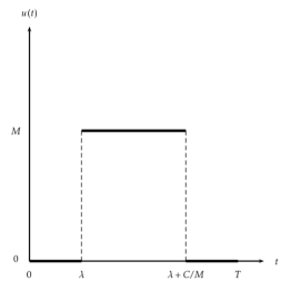
Let T𝑇T, C𝐶C, M𝑀M be three positive numbers and assume that T>C/M𝑇𝐶𝑀T>C/M (in other words that the horizon of time is large enough). Any solution u𝑢u to (𝒫reducedsubscript𝒫reduced\mathcal{P}_{\text{reduced}}) satisfies 0Tu(t)𝑑t=Csuperscriptsubscript0𝑇superscript𝑢𝑡differential-d𝑡𝐶\int_{0}^{T}u^{*}(t)dt=C and is bang-bang (i.e. equal a.e. to 0 or M𝑀M).

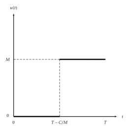
If Mmaxp[0,θ](f(p)g(p))𝑀subscript𝑝0𝜃𝑓𝑝𝑔𝑝\displaystyle M\leqslant\max_{p\in[0,\theta]}\left(-\frac{f(p)}{g(p)}\right) then the unique solution to (𝒫reducedsubscript𝒫reduced\mathcal{P}_{\text{reduced}}) is given by M𝟙[TC/M,T]𝑀subscript1𝑇𝐶𝑀𝑇M\mathds{1}_{[T-C/M,T]}.

Otherwise, defining

C(M)=0θMdpf(p)+Mg(p),superscript𝐶𝑀superscriptsubscript0𝜃𝑀𝑑𝑝𝑓𝑝𝑀𝑔𝑝C^{*}(M)=\int_{0}^{\theta}\frac{Mdp}{f(p)+Mg(p)}, (22)

one has

  • if C<C(M)𝐶superscript𝐶𝑀C<C^{*}(M) then the solution to (𝒫reducedsubscript𝒫reduced\mathcal{P}_{\text{reduced}}) is unique and equal to u=M𝟙[TC/M,T]superscript𝑢𝑀subscript1𝑇𝐶𝑀𝑇u^{*}=M\mathds{1}_{[T-C/M,T]}. In this case J0(u)>(1θ)2superscript𝐽0superscript𝑢superscript1𝜃2J^{0}(u^{*})>(1-\theta)^{2};

  • if C>C(M)𝐶superscript𝐶𝑀C>C^{*}(M) then the solution to (𝒫reducedsubscript𝒫reduced\mathcal{P}_{\text{reduced}}) is unique and equal to u=M𝟙[0,C/M]superscript𝑢𝑀subscript10𝐶𝑀u^{*}=M\mathds{1}_{[0,C/M]}. In this case J0(u)<(1θ)2superscript𝐽0superscript𝑢superscript1𝜃2J^{0}(u^{*})<(1-\theta)^{2};

  • if C=C(M)𝐶superscript𝐶𝑀C=C^{*}(M) then there is a continuum of solutions to (𝒫reducedsubscript𝒫reduced\mathcal{P}_{\text{reduced}}) given by uλ=M𝟙[λ,λ+C/M]subscriptsuperscript𝑢𝜆𝑀subscript1𝜆𝜆𝐶𝑀u^{*}_{\lambda}=M\mathds{1}_{[\lambda,\lambda+C/M]} for λ[0,TC/M]𝜆0𝑇𝐶𝑀\lambda\in[0,T-C/M], with J0(uλ)=(1θ)2superscript𝐽0subscriptsuperscript𝑢𝜆superscript1𝜃2J^{0}(u^{*}_{\lambda})=(1-\theta)^{2},

where θ𝜃\theta is given by (21).

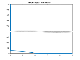
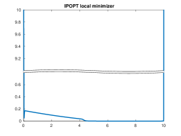
Theorem 1 is illustrated on Fig. 3.

Interpretation.

Theorem 1 implies that the best release protocol in the framework of the frequency model (15) consists in a single release phase, either at the beginning of the time frame or at the end. This result may be interpreted as follows : If the amount of mosquitoes available is enough to cross the threshold θ𝜃\theta, then it is preferable to make the maximum effort at the beginning of the time protocol, since it is clear from the differential equation (15) satisfied by the frequency p𝑝p, that p𝑝p is increasing whenever p>θ𝑝𝜃p>\theta even when u=0𝑢0u=0 (thus it is interesting to cross this threshold as soon as possible). On the contrary, if the amount of mosquitoes is not enough for p𝑝p to reach the threshold θ𝜃\theta, then p<θ𝑝𝜃p<\theta and p𝑝p is decreasing when u=0𝑢0u=0. In this case, the optimum is achieved acting at the end of the time frame to avoid p𝑝p to decrease888Note that under the same assumptions, the same conclusion holds for any problem derived from (𝒫reducedsubscript𝒫reduced\mathcal{P}_{\text{reduced}}) by changing the Cauchy data p(0)=0𝑝00p(0)=0 in (15) by an arbitrary value in [0,1)01[0,1). Therefore we can state that in general, if the threshold cannot be reached, then it is best to act only at the end of the time frame. This fact ultimately relies on the special variations of f/g𝑓𝑔f/g, see the proof of Lemma 7.. To the best our knowledge, such a “jump” of optimizers is not standard in optimal control theory. Nevertheless, we point out reference [22] where a close phenomenon is observed for issue of minimizing with respect to the domain the principal eigenvalue of an elliptic operator with Robin boundary conditions of the kind nu+βu=0subscript𝑛𝑢𝛽𝑢0\partial_{n}u+\beta u=0, where β𝛽\beta is a non-negative constant. Indeed, in this problem, two distinct families of optimizers can arise, depending of whether β𝛽\beta is larger ou smaller than a threshold value β>0superscript𝛽0\beta^{*}>0.

To what extent must this strategy be adapted when ε>0𝜀0\varepsilon>0 is small but nonzero (i.e. in the real situation where fecundity is large but finite)? Numerical results in Section 3.2 begin to answer this challenging question.

The proof relies on several intermediary lemmas which we state and prove below.

In view of stating the (necessary) first order optimality conditions for Problem (𝒫reducedsubscript𝒫reduced\mathcal{P}_{\text{reduced}}), let us compute the derivative of J0superscript𝐽0J^{0}. Let us introduce the adjoint state q𝑞q defined by

q˙=(f(p)+ug(p))q on (0,T),q(T)=2(1p(T)).formulae-sequence˙𝑞superscript𝑓𝑝𝑢superscript𝑔𝑝𝑞 on 0𝑇𝑞𝑇21𝑝𝑇-\dot{q}=\big{(}f^{\prime}(p)+ug^{\prime}(p)\big{)}q\text{ on }(0,T),\qquad q(T)=-2(1-p(T)). (23)

Standard arguments yield existence and uniqueness of a solution for System (23). Moreover, since 0<p()<10𝑝10<p(\cdot)<1, we deduce that q()<0𝑞0q(\cdot)<0 on [0,T]0𝑇[0,T].

Lemma 4.

Let u𝒰T,C,M𝑢subscript𝒰𝑇𝐶𝑀u\in\mathcal{U}_{T,C,M}. Then, for every admissible perturbation999More precisely, we call “admissible perturbation” any element of the tangent cone 𝒯u,𝒰T,C,Msubscript𝒯𝑢subscript𝒰𝑇𝐶𝑀\mathcal{T}_{u,\mathcal{U}_{T,C,M}} to the set 𝒰T,C,Msubscript𝒰𝑇𝐶𝑀\mathcal{U}_{T,C,M} at u𝑢u. The cone 𝒯u,𝒰T,C,Msubscript𝒯𝑢subscript𝒰𝑇𝐶𝑀\mathcal{T}_{u,\mathcal{U}_{T,C,M}} is the set of functions hL(0,T)superscript𝐿0𝑇h\in L^{\infty}(0,T) such that, for any sequence of positive real numbers εnsubscript𝜀𝑛\varepsilon_{n} decreasing to 00, there exists a sequence of functions hnL(0,T)subscript𝑛superscript𝐿0𝑇h_{n}\in L^{\infty}(0,T) converging to hh as n+𝑛n\rightarrow+\infty, and u+εnhn𝒰T,C,M𝑢subscript𝜀𝑛subscript𝑛subscript𝒰𝑇𝐶𝑀u+\varepsilon_{n}h_{n}\in\mathcal{U}_{T,C,M} for every nIN𝑛INn\in\mathrm{I\kern-2.10007ptN} (see e.g. [9]). hh, the Gâteaux-derivative of J0superscript𝐽0J^{0} at u𝑢u in the direction hh reads

dJ0(u),h=0Th(t)q(t)g(p(t))𝑑t.𝑑superscript𝐽0𝑢superscriptsubscript0𝑇𝑡𝑞𝑡𝑔𝑝𝑡differential-d𝑡\langle dJ^{0}(u),h\rangle=\int_{0}^{T}h(t)q(t)g(p(t))\,dt.

where p𝑝p and q𝑞q denote respectively the solutions to the problem (15) and the adjoint equation (23).

Proof.

Let hh be an admissible perturbation of u𝑢u (see Footnote 9). The Gâteaux-differentiability of J0superscript𝐽0J^{0} is standard and follows from the differentiability of the mapping 𝒰T,C,Mupcontainssubscript𝒰𝑇𝐶𝑀𝑢maps-to𝑝\mathcal{U}_{T,C,M}\ni u\mapsto p, where p𝑝p denotes the unique solution of (15), itself deriving from the application of the implicit function theorem combined with variational arguments.
Let us then compute the Gâteaux-derivative of J0superscript𝐽0J^{0} at u𝑢u in the direction hh, defined by

dJ0(u),h=limε0J0(u+εh)J0(u)ε.𝑑superscript𝐽0𝑢subscript𝜀0superscript𝐽0𝑢𝜀superscript𝐽0𝑢𝜀\langle dJ^{0}(u),h\rangle=\lim_{\varepsilon\to 0}\frac{J^{0}(u+\varepsilon h)-J^{0}(u)}{\varepsilon}.

Let p𝑝p be the solution to Eq. (4) and let us introduce δp𝛿𝑝\delta p, the Gâteaux-differential of p𝑝p at u𝑢u in the direction hh. Straightforward computations yield that δp𝛿𝑝\delta p solves the linearized problem to (4),

δp˙(t)=f(p)δp+ug(p)δp+hg(p),δp(0)=0.formulae-sequence˙𝛿𝑝𝑡superscript𝑓𝑝𝛿𝑝𝑢superscript𝑔𝑝𝛿𝑝𝑔𝑝𝛿𝑝00\dot{\delta p}(t)=f^{\prime}(p)\delta p+ug^{\prime}(p)\delta p+hg(p),\qquad\delta p(0)=0.

Furthermore, differentiating the criterion J0superscript𝐽0J^{0} yields dJ0(u),h=δp(T)(1p(T))𝑑superscript𝐽0𝑢𝛿𝑝𝑇1𝑝𝑇\langle dJ^{0}(u),h\rangle=-\delta p(T)(1-p(T)). Let us multiply Eq. (3.1) by q𝑞q and then integrate by parts on (0,T)0𝑇(0,T). One gets

0Tq˙(t)δp(t)𝑑t=δp(T)q(T)+0T(f(t)+ug(t))δp(t)q(t)𝑑t+0Th(t)g(p(t))q(t)𝑑t,superscriptsubscript0𝑇˙𝑞𝑡𝛿𝑝𝑡differential-d𝑡𝛿𝑝𝑇𝑞𝑇superscriptsubscript0𝑇superscript𝑓𝑡𝑢superscript𝑔𝑡𝛿𝑝𝑡𝑞𝑡differential-d𝑡superscriptsubscript0𝑇𝑡𝑔𝑝𝑡𝑞𝑡differential-d𝑡\displaystyle-\int_{0}^{T}\dot{q}(t)\delta p(t)\,dt=-\delta p(T)q(T)+\int_{0}^{T}(f^{\prime}(t)+ug^{\prime}(t))\delta p(t)q(t)\,dt+\int_{0}^{T}h(t)g(p(t))q(t)\,dt,

which reduces to

δp(T)q(T)=0Th(t)g(p(t))q(t)𝑑t.𝛿𝑝𝑇𝑞𝑇superscriptsubscript0𝑇𝑡𝑔𝑝𝑡𝑞𝑡differential-d𝑡\delta p(T)q(T)=\int_{0}^{T}h(t)g(p(t))q(t)\,dt.

By using the terminal condition on q𝑞q, we obtain

dJ0(u),h=2(1p(T))δp(T)=q(T)δp(T),𝑑superscript𝐽0𝑢21𝑝𝑇𝛿𝑝𝑇𝑞𝑇𝛿𝑝𝑇\langle dJ^{0}(u),h\rangle=-2(1-p(T))\delta p(T)=q(T)\delta p(T),

where q𝑞q is the solution to the adjoint equation (23). Then, we compute

0=0Tδp(q˙+f(p)q+ug(p)q)𝑑t=δp(T)q(T)δp(0)q(0)0Th(t)q(t)g(p(t))𝑑t,0superscriptsubscript0𝑇𝛿𝑝˙𝑞𝑓𝑝𝑞𝑢superscript𝑔𝑝𝑞differential-d𝑡𝛿𝑝𝑇𝑞𝑇𝛿𝑝0𝑞0superscriptsubscript0𝑇𝑡𝑞𝑡𝑔𝑝𝑡differential-d𝑡\displaystyle 0=\int_{0}^{T}\delta p(\dot{q}+f(p)q+ug^{\prime}(p)q)\,dt=\delta p(T)q(T)-\delta p(0)q(0)-\int_{0}^{T}h(t)q(t)g(p(t))\,dt,

and it follows that

dJ0(u),h=0Th(t)q(t)g(p(t))𝑑t.𝑑superscript𝐽0𝑢superscriptsubscript0𝑇𝑡𝑞𝑡𝑔𝑝𝑡differential-d𝑡\langle dJ^{0}(u),h\rangle=\int_{0}^{T}h(t)q(t)g(p(t))\,dt.

We now prove that the L1superscript𝐿1L^{1} constraint on the control u𝑢u is saturated.

Lemma 5.

If usuperscript𝑢u^{*} solves the optimization problem (𝒫reducedsubscript𝒫reduced\mathcal{P}_{\text{reduced}}), then 0Tu(t)𝑑t=min(C,TM)superscriptsubscript0𝑇superscript𝑢𝑡differential-d𝑡𝐶𝑇𝑀\displaystyle\int_{0}^{T}u^{*}(t)\,dt=\min(C,TM).

Proof.

Let us argue by contradiction, assuming the existence of a positive number κ𝜅\kappa and a set (0,T)0𝑇\mathcal{I}\subset(0,T) of positive Lebesgue measure such that 0uMκ0superscript𝑢𝑀𝜅0\leqslant u^{*}\leqslant M-\kappa on \mathcal{I} and 0Tu(t)𝑑t<Csuperscriptsubscript0𝑇superscript𝑢𝑡differential-d𝑡𝐶\int_{0}^{T}u^{*}(t)\,dt<C. Then, there exists a positive function hh in L(0,T)superscript𝐿0𝑇L^{\infty}(0,T) such that u+hsuperscript𝑢u^{*}+h belongs to 𝒰T,C,Msubscript𝒰𝑇𝐶𝑀\mathcal{U}_{T,C,M}. Moreover, according to Lemma 4, one has

limε0J0(u+εh)J0(u)ε=0Th(t)q(t)g(p(t))𝑑t<0,subscript𝜀0superscript𝐽0superscript𝑢𝜀superscript𝐽0superscript𝑢𝜀superscriptsubscript0𝑇𝑡𝑞𝑡𝑔𝑝𝑡differential-d𝑡0\lim_{\varepsilon\searrow 0}\frac{J^{0}(u^{*}+\varepsilon h)-J^{0}(u^{*})}{\varepsilon}=\int_{0}^{T}h(t)q(t)g(p(t))\,dt<0,

where p𝑝p and q𝑞q denote here the solutions of Eq. (15) and (23) associated to u=u𝑢superscript𝑢u=u^{*}, by using the positivity of hh and g𝑔g, and the negativity of the adjoint state q𝑞q. This is in contradiction with the optimality of usuperscript𝑢u^{*} and therefore, either u=Msuperscript𝑢𝑀u^{*}=M a.e. (which arises if, and only if TMC𝑇𝑀𝐶TM\leqslant C) or 0Tu(t)𝑑t=Csuperscriptsubscript0𝑇superscript𝑢𝑡differential-d𝑡𝐶\int_{0}^{T}u^{*}(t)\,dt=C. The expected conclusion follows. ∎

Lemma 6.

Let u𝒰T,C,M𝑢subscript𝒰𝑇𝐶𝑀u\in\mathcal{U}_{T,C,M} be a solution of Problem (𝒫reducedsubscript𝒫reduced\mathcal{P}_{\text{reduced}}). Define the switching function w𝑤w by w(t)=g(p(t))q(t)𝑤𝑡𝑔𝑝𝑡𝑞𝑡w(t)=g(p(t))q(t) for all t[0,T]𝑡0𝑇t\in[0,T], where p𝑝p and q𝑞q denote here the solutions of Eq. (15) and (23) associated to u=u𝑢superscript𝑢u=u^{*}. There exists Λ<0Λ0\Lambda<0 such that

  • u(t)=Mw(t)Λ𝑢𝑡𝑀𝑤𝑡Λu(t)=M\Rightarrow w(t)\leqslant\Lambda,

  • 0<u(t)<Mw(t)=Λ0𝑢𝑡𝑀𝑤𝑡Λ0<u(t)<M\Rightarrow w(t)=\Lambda,

  • u(t)=0w(t)Λ𝑢𝑡0𝑤𝑡Λu(t)=0\Rightarrow w(t)\geqslant\Lambda,

each equality being understood up to a zero Lebesgue-measure set.

Proof.

Introduce the Lagrangian function \mathcal{L} associated to Problem (𝒫reducedsubscript𝒫reduced\mathcal{P}_{\text{reduced}}), defined by

:𝒰T,C,M×IR(u,Λ)J0(u)Λ(0Tu(t)𝑑tC).:containssubscript𝒰𝑇𝐶𝑀IR𝑢Λmaps-tosuperscript𝐽0𝑢Λsuperscriptsubscript0𝑇𝑢𝑡differential-d𝑡𝐶\mathcal{L}:\mathcal{U}_{T,C,M}\times\mathrm{I\kern-2.10007ptR}\ni(u,\Lambda)\mapsto J^{0}(u)-\Lambda\left(\int_{0}^{T}u(t)\;dt-C\right).

Standard arguments enable to show the existence of a Lagrange multiplier ΛΛ\Lambda such that (u,Λ)𝑢Λ(u,\Lambda) is a saddle-point of the Lagrangian functional \mathcal{L}. Moreover, according to Lemma 5 and since T>C/M𝑇𝐶𝑀T>C/M, we have necessarily 0Tu=Csuperscriptsubscript0𝑇𝑢𝐶\int_{0}^{T}u=C.

Let x0subscript𝑥0x_{0} be a density-one point of {u=M}𝑢𝑀\{u=M\}. Let (Gn)nINsubscriptsubscript𝐺𝑛𝑛IN(G_{n})_{n\in\mathrm{I\kern-1.47005ptN}} be a sequence of measurable subsets with Gnsubscript𝐺𝑛G_{n} included in {u=M}𝑢𝑀\{u=M\} and containing x0subscript𝑥0x_{0}. Let us consider h=𝟙Gnsubscript1subscript𝐺𝑛h=\mathds{1}_{G_{n}} and notice that uηh𝑢𝜂u-\eta h belongs to 𝒰T,C,Msubscript𝒰𝑇𝐶𝑀\mathcal{U}_{T,C,M} whenever η𝜂\eta is small enough. Writing

(uηh,Λ)(u,Λ),𝑢𝜂Λ𝑢Λ\mathcal{L}(u-\eta h,\Lambda)\geqslant\mathcal{L}(u,\Lambda),

dividing this inequality by η𝜂\eta and letting η𝜂\eta go to 0, it follows that

dJ0(u),h+Λ0Th(t)𝑑t0,𝑑superscript𝐽0𝑢Λsuperscriptsubscript0𝑇𝑡differential-d𝑡0-\langle dJ^{0}(u),h\rangle+\Lambda\int_{0}^{T}h(t)\,dt\geqslant 0,

or equivalently that

Gnq(t)g(p(t))+Λ|Gn|0,subscriptsubscript𝐺𝑛𝑞𝑡𝑔𝑝𝑡Λsubscript𝐺𝑛0-\int_{G_{n}}q(t)g(p(t))+\Lambda|G_{n}|\geqslant 0,

according to Lemma 4. Dividing this inequality by |Gn|subscript𝐺𝑛|G_{n}| and letting Gnsubscript𝐺𝑛G_{n} shrink to {x0}subscript𝑥0\{x_{0}\} as n+𝑛n\to+\infty shows the first point of Lemma 6, according to the Lebesgue Density Theorem. The proof of the third point is similar, and consists in considering perturbations of the form u+ηh𝑢𝜂u+\eta h where hh denotes a positive admissible perturbation of u𝑢u supported in {u(t)=0}𝑢𝑡0\{u(t)=0\}. Finally, the proof of the second point follows the same lines, by considering bilateral perturbations of the form u±ηhplus-or-minus𝑢𝜂u\pm\eta h where hh denotes an admissible perturbation of u𝑢u supported in {0<u(t)<M}0𝑢𝑡𝑀\{0<u(t)<M\}. ∎

Lemma 7.

Let u𝒰T,C,M𝑢subscript𝒰𝑇𝐶𝑀u\in\mathcal{U}_{T,C,M} be a solution of Problem (𝒫reducedsubscript𝒫reduced\mathcal{P}_{\text{reduced}}) and let p𝑝p and q𝑞q be the solutions of Eq. (15) and (23) associated to u𝑢u.

Under the assumption (6):

  • if Mmax[0,1]f/g𝑀subscript01𝑓𝑔M\leqslant\max_{[0,1]}-f/g, then u𝑢u is bang-bang.

  • if M>max[0,1]f/g𝑀subscript01𝑓𝑔M>\max_{[0,1]}-f/g, u𝑢u is either bang-bang or constant and equal to f(p)/g(p)𝑓superscript𝑝𝑔superscript𝑝-f(p^{*})/g(p^{*}) (the latter case may occur only if C=Tf(p)/g(p)𝐶𝑇𝑓superscript𝑝𝑔superscript𝑝C=-Tf(p^{*})/g(p^{*})).

Proof.

Similarly to the statement of Lemma 6, let us introduce the function w𝑤w defined by

w(t)=q(t)gp(t).𝑤𝑡𝑞𝑡𝑔𝑝𝑡w(t)=q(t)g\circ p(t).

for all t[0,T]𝑡0𝑇t\in[0,T]. In optimal control theory, w𝑤w is the so-called switching function.

Let us differentiate w𝑤w. We get

dwdt(t)𝑑𝑤𝑑𝑡𝑡\displaystyle\frac{dw}{dt}(t) =q(t)g(t)+p(t)g(t)q(t)absentsuperscript𝑞𝑡𝑔𝑡superscript𝑝𝑡superscript𝑔𝑡𝑞𝑡\displaystyle=q^{\prime}(t)g(t)+p^{\prime}(t)g^{\prime}(t)q(t)
=(f(t)u(t)g(t))g(t)q(t)+(f(t)+u(t)g(t))g(t)q(t)absentsuperscript𝑓𝑡𝑢𝑡superscript𝑔𝑡𝑔𝑡𝑞𝑡𝑓𝑡𝑢𝑡𝑔𝑡superscript𝑔𝑡𝑞𝑡\displaystyle=(-f^{\prime}(t)-u(t)g^{\prime}(t))g(t)q(t)+(f(t)+u(t)g(t))g^{\prime}(t)q(t)
=q(t)(f(p(t))g(p(t))f(p(t))g(p(t))).absent𝑞𝑡𝑓𝑝𝑡superscript𝑔𝑝𝑡superscript𝑓𝑝𝑡𝑔𝑝𝑡\displaystyle=q(t)\big{(}f(p(t))g^{\prime}(p(t))-f^{\prime}(p(t))g(p(t))\big{)}.

Combining this computation with Remark 2 below yields the existence of a unique real number p(0,1)superscript𝑝01p^{*}\in(0,1) such that (f/g)(p)=0superscript𝑓𝑔superscript𝑝0(f/g)^{\prime}(p^{*})=0. Now, it follows from Lemma 6 that one has p(t)=0superscript𝑝𝑡0p^{\prime}(t)=0 on {0<u<M}0𝑢𝑀\{0<u<M\} (see e.g. [17, Remark 3.1.10] for a proof of this fact). Plugging this equality in the main equation of (15) yields that

u(t)=f(p)g(p)on{0<u<M}.𝑢𝑡𝑓superscript𝑝𝑔superscript𝑝on0𝑢𝑀u(t)=-\frac{f(p^{*})}{g(p^{*})}\qquad\text{on}\quad\{0<u<M\}.

At this step, we have proved that the optimal control u𝑢u satisfies u(t){0,f(p)/g(p),M}𝑢𝑡0𝑓superscript𝑝𝑔superscript𝑝𝑀u(t)\in\{0,-f(p^{*})/g(p^{*}),M\} for a.e. t(0,T)𝑡0𝑇t\in(0,T).

Let us distinguish between two cases:

  • if Mmaxp¯[0,θ][f(p¯)/g(p¯)]𝑀subscript¯𝑝0𝜃𝑓¯𝑝𝑔¯𝑝M\leqslant\max_{\bar{p}\in[0,\theta]}[-f(\bar{p})/g(\bar{p})] (note that the maximum of f/g𝑓𝑔-f/g over [0,θ]0𝜃[0,\theta] is the maximum of f/g𝑓𝑔-f/g over (0,1)01(0,1)), then, one gets immediately that |{0<u<M}|=00𝑢𝑀0|\{0<u<M\}|=0 (else, the necessary optimality conditions would show that u𝑢u does not belong to the admissible set 𝒰T,C,Msubscript𝒰𝑇𝐶𝑀\mathcal{U}_{T,C,M}).

  • else, if M>maxp¯[0,θ][f(p¯)/g(p¯)]𝑀subscript¯𝑝0𝜃𝑓¯𝑝𝑔¯𝑝M>\max_{\bar{p}\in[0,\theta]}[-f(\bar{p})/g(\bar{p})], we claim that

    {0<u<M}={t(0,T)p(t)=p}={t(0,T)u(t)=f(p)g(p)}.0𝑢𝑀conditional-set𝑡0𝑇𝑝𝑡superscript𝑝conditional-set𝑡0𝑇𝑢𝑡𝑓superscript𝑝𝑔superscript𝑝\{0<u<M\}=\left\{t\in(0,T)\mid p(t)=p^{*}\right\}=\left\{t\in(0,T)\mid u(t)=-\frac{f(p^{*})}{g(p^{*})}\right\}. (24)

    Indeed, according to Lemma 6, one has

    {0<u<M}{t(0,T)p(t)=p}{t(0,T)u(t)=f(p)g(p)}.0𝑢𝑀conditional-set𝑡0𝑇𝑝𝑡superscript𝑝conditional-set𝑡0𝑇𝑢𝑡𝑓superscript𝑝𝑔superscript𝑝\{0<u<M\}\subset\left\{t\in(0,T)\mid p(t)=p^{*}\right\}\subset\left\{t\in(0,T)\mid u(t)=-\frac{f(p^{*})}{g(p^{*})}\right\}.

    By using that u(t){0,f(p)/g(p),M}𝑢𝑡0𝑓superscript𝑝𝑔superscript𝑝𝑀u(t)\in\{0,-f(p^{*})/g(p^{*}),M\} for a.e. t(0,T)𝑡0𝑇t\in(0,T), if u(t)=f(p)g(p)𝑢𝑡𝑓superscript𝑝𝑔superscript𝑝u(t)=-\frac{f(p^{*})}{g(p^{*})} on a positive measure set, then u(t)<M𝑢𝑡𝑀u(t)<M because of the above assumption on M𝑀M and furthermore u(t)>0𝑢𝑡0u(t)>0 (else, f(p)=0𝑓superscript𝑝0f(p^{*})=0 which is impossible since p(0,θ)superscript𝑝0𝜃p^{*}\in(0,\theta)). Hence, one has {t(0,T)u(t)=f(p)g(p)}{0<u<M}conditional-set𝑡0𝑇𝑢𝑡𝑓superscript𝑝𝑔superscript𝑝0𝑢𝑀\left\{t\in(0,T)\mid u(t)=-\frac{f(p^{*})}{g(p^{*})}\right\}\subset\{0<u<M\}, whence the claim.

    Using that {0<u<M}={p=p}0𝑢𝑀𝑝superscript𝑝\{0<u<M\}=\{p=p^{*}\} and since {t(0,T)w(t)=Λ}{t(0,T)p(t)=p}conditional-set𝑡0𝑇𝑤𝑡Λconditional-set𝑡0𝑇𝑝𝑡superscript𝑝\{t\in(0,T)\mid w(t)=\Lambda\}\subset\left\{t\in(0,T)\mid p(t)=p^{*}\right\}, it follows that

    {w=Λ}={0<u<M},{u=M}={w<Λ}and{u=0}={w>Λ}.formulae-sequence𝑤Λ0𝑢𝑀formulae-sequence𝑢𝑀𝑤Λand𝑢0𝑤Λ\{w=\Lambda\}=\{0<u<M\},\quad\{u=M\}=\{w<\Lambda\}\quad\text{and}\quad\{u=0\}=\{w>\Lambda\}.

    Between 00 and 111, f𝑓f changes sign only once, at θ𝜃\theta. In addition, the switching function w𝑤w is decreasing if p(t)<p𝑝𝑡superscript𝑝p(t)<p^{*} and increasing if p(t)>p𝑝𝑡superscript𝑝p(t)>p^{*}, since it is positively proportional to (f/g)superscript𝑓𝑔(f/g)^{\prime}, which changes sign only once, and f/g𝑓𝑔f/g changes sign only once, and is decreasing at 00, so (f/g)superscript𝑓𝑔(f/g)^{\prime} has the same sign as pp𝑝superscript𝑝p-p^{*}. Notice that necessarily, θp𝜃superscript𝑝\theta\geqslant p^{*}. Indeed, f/g𝑓𝑔f/g is decreasing on (0,p)0superscript𝑝(0,p^{*}) and equal to 00 at 00 and θ𝜃\theta.

    Let t¯¯𝑡\bar{t} be a switching point from u=f(p)g(p)𝑢𝑓superscript𝑝𝑔superscript𝑝u=-\frac{f(p^{*})}{g(p^{*})} to u=0𝑢0u=0. Such a definition makes sense by interpreting t¯¯𝑡\bar{t} as a well-chosen endpoint of a connected component of {u=0}𝑢0\{u=0\}, which is an open set.

    According to the considerations above, p𝑝p must decrease since p<θsuperscript𝑝𝜃p^{*}<\theta, so p(t)<p𝑝𝑡superscript𝑝p(t)<p^{*} at t¯¯𝑡\bar{t}, and therefore w𝑤w must decrease at t¯¯𝑡\bar{t}. But this is in contradiction with the necessary optimality condition of Lemma 6. If at t¯¯𝑡\bar{t} we have u=M𝑢𝑀u=M then p𝑝p must increase if M𝑀M is large enough. Then w𝑤w must increase, and again this is in contradiction with Lemma 6. Hence |I|=0𝐼0|I|=0 or |I|=T𝐼𝑇|I|=T. But I=[0,T]𝐼0𝑇I=[0,T] is admissible if and only if Tf(p)/g(p)=C𝑇𝑓superscript𝑝𝑔superscript𝑝𝐶-Tf(p^{*})/g(p^{*})=C.

At this step, we have shown that any optimal control u𝑢u is bang-bang whenever T>C/M𝑇𝐶𝑀T>C/M. It remains to determine optimal configurations among bang-bang functions, which is the goal of what follows.

Let us define pMsubscript𝑝𝑀p_{M} as the solution of

dpMdt=f(pM)+Mg(pM),pM(0)=0.formulae-sequence𝑑subscript𝑝𝑀𝑑𝑡𝑓subscript𝑝𝑀𝑀𝑔subscript𝑝𝑀subscript𝑝𝑀00\frac{dp_{M}}{dt}=f(p_{M})+Mg(p_{M}),\quad p_{M}(0)=0.

Assume that M>maxp[0,θ]f(p)g(p)𝑀subscript𝑝0𝜃𝑓𝑝𝑔𝑝M>\max_{p\in[0,\theta]}-\frac{f(p)}{g(p)}. Then dpMdt=f(pM)+Mg(pM)>0.𝑑subscript𝑝𝑀𝑑𝑡𝑓subscript𝑝𝑀𝑀𝑔subscript𝑝𝑀0\frac{dp_{M}}{dt}=f(p_{M})+Mg(p_{M})>0. Introduce the function GMsubscript𝐺𝑀G_{M} defined by GM(p)=1f(p)+Mg(p)subscriptsuperscript𝐺𝑀𝑝1𝑓𝑝𝑀𝑔𝑝G^{\prime}_{M}(p)=\frac{1}{f(p)+Mg(p)} and GM(0)=0subscript𝐺𝑀00G_{M}(0)=0. Then, GMsubscript𝐺𝑀G_{M} is an increasing function and we have

GM(pM(t))=GM(pM(t0))+tt0, and GM(pM(C/M))=CM.formulae-sequencesubscript𝐺𝑀subscript𝑝𝑀𝑡subscript𝐺𝑀subscript𝑝𝑀subscript𝑡0𝑡subscript𝑡0 and subscript𝐺𝑀subscript𝑝𝑀𝐶𝑀𝐶𝑀G_{M}(p_{M}(t))=G_{M}(p_{M}(t_{0}))+t-t_{0},\quad\mbox{ and }\quad G_{M}(p_{M}(C/M))=\frac{C}{M}.

The use of all these results allows us to prove Theorem 1.

Proof of Theorem 1.

We split the proof into three cases:

  • Case pM(C/M)<θsubscript𝑝𝑀𝐶𝑀𝜃p_{M}(C/M)<\theta. This condition is equivalent to GM(pM(C/M))<GM(θ)subscript𝐺𝑀subscript𝑝𝑀𝐶𝑀subscript𝐺𝑀𝜃G_{M}(p_{M}(C/M))<G_{M}(\theta) (since GMsubscript𝐺𝑀G_{M} is increasing). By Lemma 7, the control u𝑢u is bang-bang and the set where u=M𝑢𝑀u=M is open, (since from Lemma 6, it is the set of interval on which g(p)q<Λ𝑔𝑝𝑞Λg(p)q<\Lambda). Consider that u𝑢u is given by u(t)=MiIN𝟙(t2i+1,t2i+2)𝑢𝑡𝑀subscript𝑖INsubscript1subscript𝑡2𝑖1subscript𝑡2𝑖2u(t)=M\sum_{i\in\mathrm{I\kern-1.47005ptN}}\mathds{1}_{(t_{2i+1},t_{2i+2})}, where t0=0subscript𝑡00t_{0}=0 and (ti)iINsubscriptsubscript𝑡𝑖𝑖IN(t_{i})_{i\in\mathrm{I\kern-1.47005ptN}} is a non-decreasing sequence of times in [0,T]0𝑇[0,T]. We denote by p𝑝p the corresponding solution to (4).

    We want to compare with the control u¯=M𝟙[TC/M,T]¯𝑢𝑀subscript1𝑇𝐶𝑀𝑇\bar{u}=M\mathds{1}_{[T-C/M,T]}, for which the corresponding solution to (4) is denoted p¯¯𝑝\bar{p}. Then, p¯(T)=GM1(C/M)¯𝑝𝑇superscriptsubscript𝐺𝑀1𝐶𝑀\bar{p}(T)=G_{M}^{-1}(C/M).

    Let us show that p(T)<p¯(T)=GM1(C/M)𝑝𝑇¯𝑝𝑇superscriptsubscript𝐺𝑀1𝐶𝑀p(T)<\bar{p}(T)=G_{M}^{-1}(C/M). We use an induction to prove that for all iIN𝑖INi\in\mathrm{I\kern-2.10007ptN}, p(t2i)<GM1(C/M)𝑝subscript𝑡2𝑖subscriptsuperscript𝐺1𝑀𝐶𝑀p(t_{2i})<G^{-1}_{M}(C/M). Indeed, if we assume that for a iIN𝑖superscriptINi\in\mathrm{I\kern-2.10007ptN}^{*}, we have for every ki𝑘𝑖k\leqslant i, p(t2k)<GM1(C/M)<θ𝑝subscript𝑡2𝑘superscriptsubscript𝐺𝑀1𝐶𝑀𝜃p(t_{2k})<G_{M}^{-1}(C/M)<\theta. Then, on (t2i,t2i+1)subscript𝑡2𝑖subscript𝑡2𝑖1(t_{2i},t_{2i+1}), we solve the equation

    p˙=f(p),p(t2i)<θ.formulae-sequence˙𝑝𝑓𝑝𝑝subscript𝑡2𝑖𝜃\dot{p}=f(p),\qquad p(t_{2i})<\theta.

    Since f<0𝑓0f<0 on (0,θ)0𝜃(0,\theta), it implies that p𝑝p is decreasing on (t2i,t2i+1)subscript𝑡2𝑖subscript𝑡2𝑖1(t_{2i},t_{2i+1}), thus p(t2i+1)<p(t2i)𝑝subscript𝑡2𝑖1𝑝subscript𝑡2𝑖p(t_{2i+1})<p(t_{2i}). On [t2i+1,t2i+2)subscript𝑡2𝑖1subscript𝑡2𝑖2[t_{2i+1},t_{2i+2}), we have

    GM(p(t2i+2))=GM(p(t2i+1))+t2i+2t2i+1<GM(p(t2i))+t2i+2t2i+1.subscript𝐺𝑀𝑝subscript𝑡2𝑖2subscript𝐺𝑀𝑝subscript𝑡2𝑖1subscript𝑡2𝑖2subscript𝑡2𝑖1subscript𝐺𝑀𝑝subscript𝑡2𝑖subscript𝑡2𝑖2subscript𝑡2𝑖1G_{M}(p(t_{2i+2}))=G_{M}(p(t_{2i+1}))+t_{2i+2}-t_{2i+1}<G_{M}(p(t_{2i}))+t_{2i+2}-t_{2i+1}.

    By induction, we deduce that

    GM(p(t2i+2))<subscript𝐺𝑀𝑝subscript𝑡2𝑖2absent\displaystyle G_{M}(p(t_{2i+2}))< GM(p(t2i2))+t2it2i1+t2i+2t2i+1subscript𝐺𝑀𝑝subscript𝑡2𝑖2subscript𝑡2𝑖subscript𝑡2𝑖1subscript𝑡2𝑖2subscript𝑡2𝑖1\displaystyle G_{M}(p(t_{2i-2}))+t_{2i}-t_{2i-1}+t_{2i+2}-t_{2i+1}
    <\displaystyle< G(p(t0))+t2t1++t2i+2t2i+1C/M,𝐺𝑝subscript𝑡0subscript𝑡2subscript𝑡1subscript𝑡2𝑖2subscript𝑡2𝑖1𝐶𝑀\displaystyle G(p(t_{0}))+t_{2}-t_{1}+\ldots+t_{2i+2}-t_{2i+1}\leqslant C/M,

    since p(t0)=0𝑝subscript𝑡00p(t_{0})=0 and k=0i(t2k+2t2k+1)CMsuperscriptsubscript𝑘0𝑖subscript𝑡2𝑘2subscript𝑡2𝑘1𝐶𝑀\displaystyle\sum_{k=0}^{i}(t_{2k+2}-t_{2k+1})\leqslant\frac{C}{M}. We infer

    p(t2i+2)<GM1(C/M).𝑝subscript𝑡2𝑖2superscriptsubscript𝐺𝑀1𝐶𝑀p(t_{2i+2})<G_{M}^{-1}(C/M).

    This concludes the induction and the proof in this first case.

  • Case pM(C/M)>θsubscript𝑝𝑀𝐶𝑀𝜃p_{M}(C/M)>\theta. We use the same strategy and introduce the solution p𝑝p to (4) with u𝑢u given by u(t)=MiIN𝟙(t2i,t2i+1)𝑢𝑡𝑀subscript𝑖INsubscript1subscript𝑡2𝑖subscript𝑡2𝑖1u(t)=M\sum_{i\in\mathrm{I\kern-1.47005ptN}}\mathds{1}_{(t_{2i},t_{2i+1})}, where (ti)iINsubscriptsubscript𝑡𝑖𝑖IN(t_{i})_{i\in\mathrm{I\kern-1.47005ptN}} is an increasing sequence of time in [0,T]0𝑇[0,T]. We want to compare with the solution p¯¯𝑝\bar{p} for u¯=M𝟙[0,C/M]¯𝑢𝑀subscript10𝐶𝑀\bar{u}=M\mathds{1}_{[0,C/M]}.

    We first observe that since p¯(C/M)=pM(C/M)>θ¯𝑝𝐶𝑀subscript𝑝𝑀𝐶𝑀𝜃\bar{p}(C/M)=p_{M}(C/M)>\theta and f>0𝑓0f>0 on (θ,1)𝜃1(\theta,1), we have p¯¯𝑝\bar{p} increasing on [C/M,T]𝐶𝑀𝑇[C/M,T] and p¯(C/M)=GM1(C/M)¯𝑝𝐶𝑀superscriptsubscript𝐺𝑀1𝐶𝑀\bar{p}(C/M)=G_{M}^{-1}(C/M). If at time t1subscript𝑡1t_{1}, we have p(t1)<θ𝑝subscript𝑡1𝜃p(t_{1})<\theta, then on (t1,t2)subscript𝑡1subscript𝑡2(t_{1},t_{2}), p𝑝p is decreasing. Then p(t2)<p(t1)p¯(t1t0)𝑝subscript𝑡2𝑝subscript𝑡1¯𝑝subscript𝑡1subscript𝑡0p(t_{2})<p(t_{1})\leqslant\bar{p}(t_{1}-t_{0}) and we may prove as above that as long as p(t2i+1)<θ𝑝subscript𝑡2𝑖1𝜃p(t_{2i+1})<\theta, we have p(t2i+2)<p¯(k=0i(t2k+1t2k))𝑝subscript𝑡2𝑖2¯𝑝superscriptsubscript𝑘0𝑖subscript𝑡2𝑘1subscript𝑡2𝑘p(t_{2i+2})<\bar{p}\left(\sum_{k=0}^{i}(t_{2k+1}-t_{2k})\right).

    As a consequence the solution p𝑝p associated with the optimal control should satisfy p(t1)>θ𝑝subscript𝑡1𝜃p(t_{1})>\theta. Then, on (t1,T)subscript𝑡1𝑇(t_{1},T) the function p𝑝p solving (4) is increasing, thus on (t1,T)subscript𝑡1𝑇(t_{1},T), we have p>θ>p𝑝𝜃superscript𝑝p>\theta>p^{*}. Then the switch function w𝑤w is increasing. However, we have w>Λ𝑤Λw>\Lambda on (t1,t2)subscript𝑡1subscript𝑡2(t_{1},t_{2}) since u=0𝑢0u=0 from Lemma 6. Hence, it is not possible to have u=M𝑢𝑀u=M for larger times.

  • In the case where pM(C/M)=θsubscript𝑝𝑀𝐶𝑀𝜃p_{M}(C/M)=\theta. In this case, we have u=M𝟙(λ,C/M+λ)𝑢𝑀subscript1𝜆𝐶𝑀𝜆u=M\mathds{1}_{(\lambda,C/M+\lambda)} for any 0λTC/M0𝜆𝑇𝐶𝑀0\leqslant\lambda\leqslant T-C/M. Indeed, for such a function, we have p0𝑝0p\equiv 0 on [0,λ]0𝜆[0,\lambda] and pθ𝑝𝜃p\equiv\theta on [C/M+τ,T]𝐶𝑀𝜏𝑇[C/M+\tau,T]. By contradiction, assume there is an interval on which u=0𝑢0u=0 between two intervals on which u=M𝑢𝑀u=M, then on this interval p𝑝p is decreasing, and thus p𝑝p cannot reach the value θ𝜃\theta at the final time of control, by comparison.

Remark 2.

It is notable that the proof of Theorem 1 rests upon a property of the functions involved in Equation (15), namely the existence of a unique p(0,1)superscript𝑝01p^{*}\in(0,1) such that (f/g)(p)=0superscript𝑓𝑔superscript𝑝0(f/g)^{\prime}(p^{*})=0, and CTf(p)/g(p)𝐶𝑇𝑓superscript𝑝𝑔superscript𝑝C\not=-Tf(p^{*})/g(p^{*}). Indeed, letting ξ=d1b20d2b10𝜉subscript𝑑1superscriptsubscript𝑏20subscript𝑑2superscriptsubscript𝑏10\xi=\frac{d_{1}b_{2}^{0}}{d_{2}b_{1}^{0}} we have

fg(p)=Kd2(p1shpξp),(fg)(p)=Kd2(1(1shp)2ξ1).formulae-sequence𝑓𝑔𝑝𝐾subscript𝑑2𝑝1subscript𝑠𝑝𝜉𝑝superscript𝑓𝑔𝑝𝐾subscript𝑑21superscript1subscript𝑠𝑝2𝜉1\frac{f}{g}(p)=Kd_{2}\big{(}\frac{p}{1-s_{h}p}\xi-p\big{)},\quad\big{(}\frac{f}{g}\big{)}^{\prime}(p)=Kd_{2}\big{(}\frac{1}{(1-s_{h}p)^{2}}\xi-1\big{)}.

The roots of the second-order polynomial at the numerator of the right-hand side read

p±=1sh(1±ξ),subscript𝑝plus-or-minus1subscript𝑠plus-or-minus1𝜉p_{\pm}=\frac{1}{s_{h}}\big{(}1\pm\sqrt{\xi}\big{)},

so assuming (6) (i.e. ξ<1𝜉1\xi<1) yields

p=1sh(1ξ)superscript𝑝1subscript𝑠1𝜉p^{*}=\frac{1}{s_{h}}\big{(}1-\sqrt{\xi}\big{)}

(which indeed belongs to [0,θ)0𝜃[0,\theta) as a consequence of (6): from 1sh<ξ<11subscript𝑠𝜉11-s_{h}<\xi<1 it follows that 0<p<(11sh)/sh<10superscript𝑝11subscript𝑠subscript𝑠10<p^{*}<(1-\sqrt{1-s_{h}})/s_{h}<1 since sh(0,1]subscript𝑠01s_{h}\in(0,1]). On the contrary, assuming d2b10<d1b20subscript𝑑2superscriptsubscript𝑏10subscript𝑑1superscriptsubscript𝑏20d_{2}b_{1}^{0}<d_{1}b_{2}^{0} (i.e. ξ>1𝜉1\xi>1) implies that there is no such psuperscript𝑝p^{*} in [0,1]01[0,1] (and in this case the control must be bang-bang, as a consequence of Lemma 7 above).
Refer to caption
Refer to caption
Refer to caption
Figure 3: Left: solution usuperscript𝑢u^{*} in the case M>maxp[0,θ]f(p)/g(p)𝑀subscript𝑝0𝜃𝑓𝑝𝑔𝑝M>\max_{p\in[0,\theta]}-f(p)/g(p) and C>C(M)𝐶superscript𝐶𝑀C>C^{*}(M). Middle: one solution uλsubscriptsuperscript𝑢𝜆u^{*}_{\lambda} in the case M>maxp[0,θ]f(p)/g(p)𝑀subscript𝑝0𝜃𝑓𝑝𝑔𝑝M>\max_{p\in[0,\theta]}-f(p)/g(p) and C=C(M)𝐶superscript𝐶𝑀C=C^{*}(M). Right: solution usuperscript𝑢u^{*} in the case Mmaxp[0,θ]f(p)/g(p)𝑀subscript𝑝0𝜃𝑓𝑝𝑔𝑝M\leqslant\max_{p\in[0,\theta]}-f(p)/g(p) or M>maxp[0,θ]f(p)/g(p)𝑀subscript𝑝0𝜃𝑓𝑝𝑔𝑝M>\max_{p\in[0,\theta]}-f(p)/g(p) and C<C(M)𝐶superscript𝐶𝑀C<C^{*}(M). .

From Proposition 2 and Theorem 1, we provide hereafter a more precise result about the convergence of optimal values for Problem (𝒫fullsubscript𝒫full\mathcal{P}_{\text{full}}) as ε0𝜀0\varepsilon\searrow 0.

Corollary 1.

Let (uε)ε>0subscriptsuperscript𝑢𝜀𝜀0(u^{\varepsilon})_{\varepsilon>0} be a family of minimizers for Problem (𝒫fullsubscript𝒫full\mathcal{P}_{\text{full}}). Then, (uε)ε>0subscriptsuperscript𝑢𝜀𝜀0(u^{\varepsilon})_{\varepsilon>0} converges strongly in L1(0,T)superscript𝐿10𝑇L^{1}(0,T) to a solution of Problem (𝒫reducedsubscript𝒫reduced\mathcal{P}_{\text{reduced}}) as ε0𝜀0\varepsilon\searrow 0 (which is unique whenever CC(M)𝐶superscript𝐶𝑀C\neq C^{*}(M) with the notations of Theorem 1).

Proof.

According to Proposition 2, we know that (uε)ε>0subscriptsuperscript𝑢𝜀𝜀0(u^{\varepsilon})_{\varepsilon>0} converges weak star in L(0,T)superscript𝐿0𝑇L^{\infty}(0,T) to a solution of Problem (𝒫reducedsubscript𝒫reduced\mathcal{P}_{\text{reduced}}), say usuperscript𝑢u^{*}.

Since usuperscript𝑢u^{*} is an extremal point of the convex set 𝒰T,C,Msubscript𝒰𝑇𝐶𝑀\mathcal{U}_{T,C,M} to which all elements of the sequence (uε)εsubscriptsuperscript𝑢𝜀𝜀(u^{\varepsilon})_{\varepsilon} belong, it follows from [1] that the Lsuperscript𝐿L^{\infty}-weak* convergence (that is here, L1superscript𝐿1L^{1}-weak convergence) implies strong convergence in L1superscript𝐿1L^{1}, and therefore

limε00T|uε(t)u(t)|𝑑t=0.subscript𝜀0superscriptsubscript0𝑇superscript𝑢𝜀𝑡superscript𝑢𝑡differential-d𝑡0\lim_{\varepsilon\to 0}\int_{0}^{T}\lvert u^{\varepsilon}(t)-u^{*}(t)\rvert dt=0.

Finally, we conclude by observing that, whenever CC(M)𝐶superscript𝐶𝑀C\neq C^{*}(M), the solution to Problem (𝒫reducedsubscript𝒫reduced\mathcal{P}_{\text{reduced}}) is unique according to Theorem 1. ∎

3.2 Numerics

This section is devoted to computing the solution of Problem (𝒫fullsubscript𝒫full\mathcal{P}_{\text{full}}) and to illustrating the relations with its reduced version (𝒫reducedsubscript𝒫reduced\mathcal{P}_{\text{reduced}}).

All the simulations are obtained with a direct method applied to the optimal control problem (𝒫fullsubscript𝒫full\mathcal{P}_{\text{full}}), consisting in discretizing System (1), the control, and to reduce the optimal control problem to some minimization problem with constraints. To this aim, we used the open-source optimization routine from IPOPT (see [30]) combined with AMPL modeling language (see [15]). This enables the computation of a local minimizer for a discretized version of (𝒫fullsubscript𝒫full\mathcal{P}_{\text{full}}).

Choice of numerical parameters and methods.

Populations are normalized by setting K=1𝐾1K=1, and Table 1 yields the values used for the other parameters. The time-dynamics (the slow-fast system (12) depending on ε𝜀\varepsilon) are discretized with the Runge-Kutta implicit scheme Lobatto IIIC of order 222 (two stages). This scheme is asymptotic preserving in ε𝜀\varepsilon (see [16]) and allows for sound comparison of the simulations across a range of values of this parameter.

We obtain a solution 𝐧Δt(IR+)2Ndsubscript𝐧Δ𝑡superscriptsubscriptIR2subscript𝑁𝑑\mathbf{n}_{\Delta t}\in(\mathrm{I\kern-2.10007ptR}_{+})^{2N_{d}} as well as an approximate local minimizer for the discretized problem (𝒫fullsubscript𝒫full\mathcal{P}_{\text{full}}), u^ε,Δt[0,M]Ndsuperscript^𝑢𝜀Δ𝑡superscript0𝑀subscript𝑁𝑑\widehat{u}^{\varepsilon,\Delta t}\in[0,M]^{N_{d}}. Finally, note that several choices of initialization have been tested (among which constant and random ones).

Category Parameter Name Value or range
Discretization ΔtΔ𝑡\Delta t Time step [0.0004,0.0015]0.00040.0015[0.0004,0.0015]
Singular limit 1/ε1𝜀1/\varepsilon Birth rates normalization [1,2000]12000[1,2000]
Optimization T𝑇T Final time 101010
C𝐶C Maximal release number [0.15,0.75]0.150.75[0.15,0.75]
M𝑀M Maximal release flux 101010
Biology b10superscriptsubscript𝑏10b_{1}^{0} Normalized wild birth rate 111
b20superscriptsubscript𝑏20b_{2}^{0} Normalized infected birth rate 0.90.90.9
d1subscript𝑑1d_{1} Wild death rate 0.270.270.27
d2subscript𝑑2d_{2} Infected death rate 0.30.30.3
shsubscript𝑠s_{h} Cytoplasmic incompatibility level 0.90.90.9
Table 1: Parameters for the numerical resolution of (𝒫fullsubscript𝒫full\mathcal{P}_{\text{full}})

Results.

It is convenient to introduce the number of steps in the time discretization Nd=T/Δtsubscript𝑁𝑑𝑇Δ𝑡N_{d}=T/\Delta t.

For the parameters given in Table 1, we can compute the critical value C(M)superscript𝐶𝑀C^{*}(M) from Theorem 1 numerically: it is close to 0.240.240.24. Therefore we choose three values of C𝐶C (0.150.150.15, 0.40.40.4 and 0.750.750.75) both above and below this threshold, so as to get contrasting results. On Figure 4 below, solutions of Problem (𝒫fullsubscript𝒫full\mathcal{P}_{\text{full}}) are computed for these three different values of the integral bound C𝐶C and for ε=1𝜀1\varepsilon=1. We observe that the set IMΔt,κ:={k1,Nd,u^kε,ΔtMκ}assignsuperscriptsubscript𝐼𝑀Δ𝑡𝜅formulae-sequence𝑘1subscript𝑁𝑑subscriptsuperscript^𝑢𝜀Δ𝑡𝑘𝑀𝜅I_{M}^{\Delta t,\kappa}:=\{k\in\llbracket 1,N_{d}\rrbracket,\,\widehat{u}^{\varepsilon,\Delta t}_{k}\geqslant M-\kappa\} (approximating the set {u=M}𝑢𝑀\{u=M\}), for κ𝜅\kappa small enough, is made of two segments containing either 111 or Ndsubscript𝑁𝑑N_{d}. Let us denote these two segments 1,k0(Δt)1subscript𝑘0Δ𝑡\llbracket 1,k_{0}(\Delta t)\rrbracket and k1(Δt),Ndsubscript𝑘1Δ𝑡subscript𝑁𝑑\llbracket k_{1}(\Delta t),N_{d}\rrbracket. It seems that

  • a relaxation type phenomenon may occur for optimal controls meaning that the solution is not bang-bang.

  • the set IrelaxΔt,κ:={k1,Nd,κu^kε,ΔtMκ}assignsuperscriptsubscript𝐼relaxΔ𝑡𝜅formulae-sequence𝑘1subscript𝑁𝑑𝜅subscriptsuperscript^𝑢𝜀Δ𝑡𝑘𝑀𝜅I_{\textrm{relax}}^{\Delta t,\kappa}:=\{k\in\llbracket 1,N_{d}\rrbracket,\,\kappa\leqslant\widehat{u}^{\varepsilon,\Delta t}_{k}\leqslant M-\kappa\} (approximating the set {0<u<M}0𝑢𝑀\{0<u<M\}) seems to be a segment for κ𝜅\kappa small enough.

  • for small values of C𝐶C, k0=0subscript𝑘00k_{0}=0, k1=Ndsubscript𝑘1subscript𝑁𝑑k_{1}=N_{d} and there is replacement failure, suggesting that it is necessary to release a minimal number of infected mosquitoes in order to guarantee population replacement.
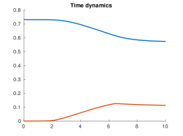
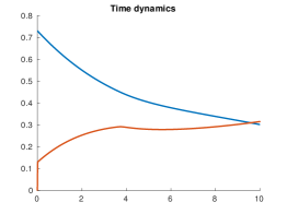
Refer to caption
Refer to caption
Refer to caption
Refer to caption
Refer to caption
Refer to caption
Figure 4: Top: time dynamics (plots of the wild mosquitoes density n1subscript𝑛1n_{1} starting from a positive value versus the Wolbachia-infected mosquitoes density n2subscript𝑛2n_{2} starting from 00). Bottom: numerical optimal control. From the left to the right: C=0.15𝐶0.15C=0.15, C=0.4𝐶0.4C=0.4 and C=0.75𝐶0.75C=0.75. The parameter ε𝜀\varepsilon is fixed to 111.
Refer to caption
Refer to caption
Refer to caption
Refer to caption
Figure 5: Case C=0.75𝐶0.75C=0.75. Top left: numerical minimum value Jε(u^ε,Δt)superscript𝐽𝜀superscript^𝑢𝜀Δ𝑡J^{\varepsilon}(\widehat{u}^{\varepsilon,\Delta t}) and Jε(u0)superscript𝐽𝜀subscriptsuperscript𝑢0J^{\varepsilon}(u^{*}_{0}) w.r.t. ε𝜀\varepsilon. Top right: relative error between the value of Jεsuperscript𝐽𝜀J^{\varepsilon} at the numerical minimizer u^ε,Δtsuperscript^𝑢𝜀Δ𝑡\widehat{u}^{\varepsilon,\Delta t} and at the exact solution usuperscript𝑢u^{*} of the asymptotic problem (𝒫reducedsubscript𝒫reduced\mathcal{P}_{\text{reduced}}) w.r.t. ε𝜀\varepsilon. Bottom left: plot of the absolute error between p^εsuperscript^𝑝𝜀\widehat{p}^{\varepsilon} and p0superscriptsubscript𝑝0p_{0}^{*}. Bottom right: L1superscript𝐿1L^{1} error between u^ε,Δtsuperscript^𝑢𝜀Δ𝑡\widehat{u}^{\varepsilon,\Delta t} and u0subscriptsuperscript𝑢0u^{*}_{0}.
Refer to caption
Refer to caption
Refer to caption
Refer to caption
Figure 6: Case C=0.15𝐶0.15C=0.15. Top left: numerical minimum value Jε(u^ε,Δt)superscript𝐽𝜀superscript^𝑢𝜀Δ𝑡J^{\varepsilon}(\widehat{u}^{\varepsilon,\Delta t}) and Jε(u0)superscript𝐽𝜀subscriptsuperscript𝑢0J^{\varepsilon}(u^{*}_{0}) w.r.t. ε𝜀\varepsilon. Top right: relative error between the value of Jεsuperscript𝐽𝜀J^{\varepsilon} at the numerical minimizer u^ε,Δtsuperscript^𝑢𝜀Δ𝑡\widehat{u}^{\varepsilon,\Delta t} and at the exact solution usuperscript𝑢u^{*} of the asymptotic problem (𝒫reducedsubscript𝒫reduced\mathcal{P}_{\text{reduced}}) w.r.t. ε𝜀\varepsilon. Bottom left: plot of the absolute error between p^εsuperscript^𝑝𝜀\widehat{p}^{\varepsilon} and p0superscriptsubscript𝑝0p_{0}^{*}. Bottom right: L1superscript𝐿1L^{1} error between u^ε,Δtsuperscript^𝑢𝜀Δ𝑡\widehat{u}^{\varepsilon,\Delta t} and u0subscriptsuperscript𝑢0u^{*}_{0}

Figures 5 and 6 are used to validate our approach of considering the asymptotic problem (𝒫reducedsubscript𝒫reduced\mathcal{P}_{\text{reduced}}) instead of the real one (𝒫fullsubscript𝒫full\mathcal{P}_{\text{full}}), with C=0.75𝐶0.75C=0.75 (leading to replacement success) and C=0.15𝐶0.15C=0.15 (leading to replacement failure), respectively. We compare the numerical values of J(u=u^ε,Δt)𝐽𝑢superscript^𝑢𝜀Δ𝑡J(u=\widehat{u}^{\varepsilon,\Delta t}) obtained either by using the direct optimization routine described above, or by choosing u=u0𝑢subscriptsuperscript𝑢0u=u^{*}_{0} as the (explicit) solution of Problem (𝒫reducedsubscript𝒫reduced\mathcal{P}_{\text{reduced}}). As expected, the ratio

Jε(u0)Jε(u^ε,Δt)Jε(u^ε,Δt)superscript𝐽𝜀subscriptsuperscript𝑢0superscript𝐽𝜀superscript^𝑢𝜀Δ𝑡superscript𝐽𝜀superscript^𝑢𝜀Δ𝑡\frac{J^{\varepsilon}(u^{*}_{0})-J^{\varepsilon}(\widehat{u}^{\varepsilon,\Delta t})}{J^{\varepsilon}(\widehat{u}^{\varepsilon,\Delta t})}

visually converges to 00 as ε0𝜀0\varepsilon\searrow 0. The bottom panels in figures 5 and 6 illustrate the convergence properties for pεsuperscript𝑝𝜀p^{\varepsilon} stated in Proposition 16, and for uεsuperscript𝑢𝜀u^{\varepsilon} stated in Corollary 1.

4 Conclusion

In this article, we proposed a strategy of Wolbachia-infected mosquitoes releases to control a simplified competitive compartmental system involving wild and infected individuals. Our approach is validated by numerical results that seem promising. Hereafter, we enumerate a list of issues that remain open and will be investigated in a future work.

Partial or complete solving of Problem (𝒫fullsubscript𝒫full\mathcal{P}_{\text{full}}).

When investigating numerically this problem (see Section 3.2), we observed several interesting properties of minimizers, at least for several relevant values of parameters: relaxation phenomena may appear (meaning that the minimizer usuperscript𝑢u^{*} is not bang-bang anymore). The set {u=M}superscript𝑢𝑀\{u^{*}=M\} seems to have two connected components meeting 0 and T𝑇T.

Asymptotic of Problem (𝒫fullsubscript𝒫full\mathcal{P}_{\text{full}}) when one makes simultaneously ε𝜀\varepsilon go to zero and M𝑀M (the pointwise upper-bound constraint on u𝑢u) go to ++\infty.

According to Theorem 1, one shows easily that making successively ε𝜀\varepsilon tend to 0 and then M𝑀M tend to ++\infty yields to a new asymptotic problem whose minimizers are a (typically unique) Dirac mass. When making simultaneously ε𝜀\varepsilon tend to 0 and then M𝑀M tend to ++\infty, the behavior of minimizers is not so clear and a careful analysis must be led to understand it.

Investigation of a more realistic model.

Coming back to the initial Wolbachia-infected mosquitoes control problem, it is likely that a model taking into account dispersal effects would provide more satisfying and workable results. To this aim, System (1) could be replaced by a more general reaction-diffusion system of partial differential equations. It is likely that numerical difficulties may arise for the related optimization problem, needing to develop an adapted approach.

Acknowledgement.

The authors were partially supported by the Project “Analysis and simulation of optimal shapes - application to life-sciences” of the Paris City Hall.

Appendix A Proof of Lemma 1

Solving the equation 𝐟(n1,n2)=0𝐟subscript𝑛1subscript𝑛20\mathbf{f}(n_{1},n_{2})=0 yields the steady states by direct computation. Let us use the notations N=(n1+n2)/K𝑁subscript𝑛1subscript𝑛2𝐾N=(n_{1}+n_{2})/K and p=n2/(n1+n2)𝑝subscript𝑛2subscript𝑛1subscript𝑛2p=n_{2}/(n_{1}+n_{2}). The Jacobian associated to the right-hand side 𝐟𝐟\mathbf{f} of the system reads

𝐉𝐚𝐜(𝐧)=(b1((1shp)(1(2p)N)+shp(1p)(1N))d1b1(1p)(sh(1p)+N(1sh))b2pNb2(1(1+p)N)d2).𝐉𝐚𝐜𝐧matrixsubscript𝑏11subscript𝑠𝑝12𝑝𝑁subscript𝑠𝑝1𝑝1𝑁subscript𝑑1subscript𝑏11𝑝subscript𝑠1𝑝𝑁1subscript𝑠subscript𝑏2𝑝𝑁subscript𝑏211𝑝𝑁subscript𝑑2\mathbf{Jac}(\mathbf{n})=\\ \begin{pmatrix}b_{1}\big{(}(1-s_{h}p)(1-(2-p)N)+s_{h}p(1-p)(1-N)\big{)}-d_{1}&-b_{1}(1-p)\big{(}s_{h}(1-p)+N(1-s_{h})\big{)}\\ -b_{2}pN&b_{2}(1-(1+p)N)-d_{2}\end{pmatrix}.

It is readily seen that the extra-diagonal terms are non-positive (and even negative if p(0,1)𝑝01p\in(0,1) and N>0𝑁0N>0). By Kamke-Muller conditions (see [19]), this implies that the system is monotone with respect to the cone IR+×IRsubscriptIRsubscriptIR\mathrm{I\kern-2.10007ptR}_{+}\times\mathrm{I\kern-2.10007ptR}_{-}, in other words it is competitive.

In particular,

𝐉𝐚𝐜(n1,0)𝐉𝐚𝐜superscriptsubscript𝑛10\displaystyle\mathbf{Jac}(n_{1}^{*},0) =((b1d1)b1+(1sh)d10b2d1/b1d2),absentmatrixsubscript𝑏1subscript𝑑1subscript𝑏11subscript𝑠subscript𝑑10subscript𝑏2subscript𝑑1subscript𝑏1subscript𝑑2\displaystyle=\begin{pmatrix}-(b_{1}-d_{1})&-b_{1}+(1-s_{h})d_{1}\\ 0&b_{2}d_{1}/b_{1}-d_{2}\end{pmatrix},
𝐉𝐚𝐜(0,n2)𝐉𝐚𝐜0superscriptsubscript𝑛2\displaystyle\mathbf{Jac}(0,n_{2}^{*}) =(b1d2(1sh)/b2d10(b2d2)(b2d2)),absentmatrixsubscript𝑏1subscript𝑑21subscript𝑠subscript𝑏2subscript𝑑10subscript𝑏2subscript𝑑2subscript𝑏2subscript𝑑2\displaystyle=\begin{pmatrix}b_{1}d_{2}(1-s_{h})/b_{2}-d_{1}&0\\ -(b_{2}-d_{2})&-(b_{2}-d_{2})\end{pmatrix},

so that conditions (5) and (6) easily yield the linear stability of (n1,0)superscriptsubscript𝑛10(n_{1}^{*},0) and (0,n2)0superscriptsubscript𝑛2(0,n_{2}^{*}). Combined with the monotonicity property of the system, we get the asymptotic stability.

Then, 𝐧Csuperscript𝐧𝐶\mathbf{n}^{C} belongs to the interior of the interval [(n1,0),(0,n2)]superscriptsubscript𝑛100superscriptsubscript𝑛2[(n_{1}^{*},0),(0,n_{2}^{*})] (for the order induced by the comparison principle recalled in Footnote 7), whose bounds are stable steady states, and there is no other steady state in the interior of this interval. Hence it must be unstable, since the dynamics of (1) is order-preserving.

At (0,0)00(0,0), we compute the directional derivative in direction (h,k)𝑘(h,k) as

D𝐟(h,k)=limt0𝐟(th,tk)t=((b1(1shkh+k)d1)h(b2d2)k),𝐷𝐟𝑘subscript𝑡0𝐟𝑡𝑡𝑘𝑡matrixsubscript𝑏11subscript𝑠𝑘𝑘subscript𝑑1subscript𝑏2subscript𝑑2𝑘D\mathbf{f}(h,k)=\lim_{t\to 0}\frac{\mathbf{f}(th,tk)}{t}=\begin{pmatrix}(b_{1}(1-s_{h}\frac{k}{h+k})-d_{1})h\\ (b_{2}-d_{2})k\end{pmatrix},

and in particular we find that the direction (0,1)01(0,1) is unstable.

References

  • [1] E. J. Balder. On equivalence of strong and weak convergence in L1subscript𝐿1L_{1}-spaces under extreme point conditions. Israel J. Math., 75(1):21–47, 1991.
  • [2] N. H. Barton and M. Turelli. Spatial waves of advance with bistable dynamics: cytoplasmic and genetic analogues of Allee effects. The American Naturalist, 178:E48–E75, 2011.
  • [3] A. Braides. A handbook of ΓΓ\Gamma-convergence. In M. Chipot and P. Quittner, editors, Handbook of Differential Equations: Stationary Partial Differential Equations, volume 3, pages 101 – 213. North-Holland, 2006.
  • [4] D. E. Campo-Duarte, D. Cardona-Salgado, and O. Vasilieva. Establishing wMelPop Wolbachia infection among wild Aedes aegypti females by optimal control approach. Appl. Math. Inf. Sci. 1, pages 1–17, (2017).
  • [5] D. E. Campo-Duarte, O. Vasilieva, D. Cardona-Salgado, and M. Svinin. Optimal control approach for establishing wMelPop Wolbachia infection among wild Aedes aegypti populations. Journal of Mathematical Biology, 76(7):1907–1950, Jun 2018.
  • [6] C. Carrère. Optimization of an in vitro chemotherapy to avoid resistant tumours. J. Theoret. Biol., 413:24–33, 2017.
  • [7] E. Caspari and G. Watson. On the evolutionary importance of cytoplasmic sterility in mosquitoes. Evolution, 13(4):568–570, 1959.
  • [8] M. H. T. Chan and P. S. Kim. Modeling a Wolbachia invasion using a slow-fast dispersal reaction-diffusion approach. Bull Math Biol, 75:1501–1523, 2013.
  • [9] R. Cominetti and J.-P. Penot. Tangent sets to unilateral convex sets. C. R. Acad. Sci. Paris Sér. I Math., 321(12):1631–1636, 1995.
  • [10] C. Curtis and T. Adak. Population replacement in culex fatigans by means of cytoplasmic incompatibility: 1. laboratory experiments with non-overlapping generations. Bulletin of the World Health Organization, 51(3):249–255, 1974.
  • [11] G. L. C. Dutra, L. M. B. dos Santos, E. P. Caragata, J. B. L. Silva, D. A. M. Villela, R. Maciel-de Freitas, and L. Andrade Moreira. From Lab to Field: the influence of urban landscapes on the invasive potential of Wolbachia in Brazilian Aedes aegypti mosquitoes. PLoS Negl Trop Dis, 9(4), 2015.
  • [12] J. Z. Farkas and P. Hinow. Structured and Unstructured Continuous Models for Wolbachia Infections. Bulletin of Mathematical Biology, 72(8):2067–2088, Nov 2010.
  • [13] A. Fenton, K. N. Johnson, J. C. Brownlie, and G. D. D. Hurst. Solving the Wolbachia paradox: modeling the tripartite interaction between host, Wolbachia, and a natural enemy. The American Naturalist, 178:333–342, 2011.
  • [14] D. A. Focks, D. G. Haile, E. Daniels, and G. A. Mount. Dynamic life table model of a container-inhabiting mosquito, aedes aegypti (l.) (diptera: Culicidae). part 1. analysis of the literature and model development. J. Med. Entomol., 30:1003–1017, 1993.
  • [15] R. Fourer. AMPL : a modeling language for mathematical programming. San Francisco, Calif. : Scientific Pr., San Francisco, Calif., 2. ed. edition, 1996.
  • [16] E. Hairer, C. Lubich, and M. Roche. Error of Runge-Kutta methods for stiff problems studied via differential algebraic equations. BIT, 28(3):678–700, 1988.
  • [17] A. Henrot and M. Pierre. Variation et optimisation de formes, volume 48. Springer-Verlag Berlin Heidelberg, 2005.
  • [18] M. Hertig and S. B. Wolbach. Studies on rickettsia-like micro-organisms in insects. The Journal of medical research, 44(3):329, 1924.
  • [19] Hirsch, M.W. and Smith, H. . Monotone dynamical systems. In Handbook of differential equations: ordinary differential equations, volume II, pages 239–257. Elsevier B. V., Amsterdam, 2005.
  • [20] A. A. Hoffmann, B. L. Montgomery, J. Popovici, I. Iturbe-Ormaetxe, P. H. Johnson, F. Muzzi, M. Greenfield, M. Durkan, Y. S. Leong, Y. Dong, H. Cook, J. Axford, A. G. Callahan, N. Kenny, C. Omodei, E. A. McGraw, P. A. Ryan, S. A. Ritchie, M. Turelli, and S. L. O’Neill. Successful establishment of Wolbachia in Aedes populations to suppress dengue transmission. Nature, 476(7361):454–457, aug 2011. 10.1038/nature10356.
  • [21] H. Hughes and N. F. Britton. Modeling the Use of Wolbachia to Control Dengue Fever Transmission. Bull. Math. Biol., 75:796–818, 2013.
  • [22] J. Lamboley, A. Laurain, G. Nadin, and Y. Privat. Properties of optimizers of the principal eigenvalue with indefinite weight and Robin conditions. Calc. Var. Partial Differential Equations, 55(6):Art. 144, 37, 2016.
  • [23] H. Laven. Eradication of Culex pipiens fatigans through Cytoplasmic Incompatibility. Nature, 216:383 EP –, 10 1967.
  • [24] R. Lees, J. Gilles, J. Hendrichs, M. Vreysen, and K. Bourtzis. Back to the future: the sterile insect technique against mosquito disease vectors. 10:156–162, 08 2015.
  • [25] M. Otero, N. Schweigmann, and H. G. Solari. A stochastic spatial dynamicl model for Aedes aegypti. Bulletin of Mathematical Biology, 70:1297–325, 2008.
  • [26] J. G. Schraiber, A. N. Kaczmarczyk, R. Kwok, M. Park, R. Silverstein, F. U. Rutaganira, T. Aggarwal, M. A. Schwemmer, C. L. Hom, R. K. Grosberg, and S. J. Schreiber. Constraints on the use of lifespan-shortening Wolbachia to control dengue fever. Journal of Theoretical Biology, 297:26 – 32, 2012.
  • [27] M. Strugarek and N. Vauchelet. Reduction to a single closed equation for 2-by-2 reaction-diffusion systems of Lotka-Volterra type. SIAM J. Appl. Math., 76(5):2060–2080, 2016.
  • [28] R. C. A. Thomé, H. M. Yang, and L. Esteva. Optimal control of aedes aegypti mosquitoes by the sterile insect technique and insecticide. Math. Biosci., 223(1):12–23, 2010.
  • [29] E. Trélat, J. Zhu, and E. Zuazua. Allee optimal control of a system in ecology. Math. Models Methods Appl. Sci., 28:1665–1697, 2018.
  • [30] A. Wächter and L. T. Biegler. On the implementation of an interior-point filter line-search algorithm for large-scale nonlinear programming. Math. Program., 106(1, Ser. A):25–57, 2006.
  • [31] T. Walker, P. H. Johnson, L. A. Moreira, I. Iturbe-Ormaetxe, F. D. Frentiu, C. J. McMeniman, Y. S. Leong, Y. Dong, J. Axford, P. Kriesner, A. L. Lloyd, S. A. Ritchie, S. L. O’Neill, and A. A. Hoffmann. The wMel Wolbachia strain blocks dengue and invades caged Aedes aegypti populations. Nature, 476:450–453, 2011.
  • [32] J. H. Werren, L. Baldo, and M. E. Clark. Wolbachia: master manipulators of invertebrate biology. Nature Review Microbiology, 6:741–751, 2008.